natural resource depletion and the resource curseintroduction curse cannot be supported when gdp...
TRANSCRIPT

NATURAL RESOURCE DEPLETION AND THE
RESOURCE CURSE
Submitted by
Linda Stokke
A thesis submitted in fulfilment of the requirementsfor the degree of Master in Economics
Department of EconomicsAdvisor: Ragnar TorvikNorway, June 2015

Abstract
This thesis studies the relationship between natural resources and economic wealth, in two
parts. Previous studies have found a negative relationship between natural resources and
economic wealth, a phenomenon known as the curse of natural resources. Later studies
reject the resource curse, in its simplest form, as their findings show a positive relation-
ship when measuring economic wealth by GDP levels instead of growth. The argument
is that the inclusion of initial GDP, when using GDP growth as measurement, will result
in biased estimates due to the short time horizon. However, a third group of studies
advocates the existence of a resource curse conditional upon institutional quality. In this
case, resource endowment only affects the economic welfare negatively if the quality of
institutions is sufficiently bad.
In this thesis the measurement of economic wealth is further expanded. Taking into
account that extraction of resources is a negative flow of the nation’s wealth gives a
better understating of the change in welfare, and removes some of the positive bias of
exploiting natural resources on economic wealth. An empirical analysis, utilizing data on
a total of 263 countries in year 2000, is conducted to find whether the resource curse is
still rejected when including depletion of natural resources to the analysis. None of the
estimation methods or model specifications in this thesis are able to confirm the exis-
tence of a resource curse, and in its simplest form the rejection is supported. Also the
conditional resource curse is rejected by the data material, meaning that countries with
poor institutions do not seem to have a more negative, or less positive, impact of natural
resources on GDP levels adjusted for depletion of natural resources than countries with
good institutions. However, be aware of the limitations of the data, in particular the
absence of a truly exogenous variable of resource endowment.
i

Acknowledgments
Though this master thesis is a result of my own work, several individuals have been of
crucial help and influence. Foremost, the analysis could not possibly have been con-
ducted without the data and do-files provided by Dr. Alexeev. For this help I am truly
thankful. The inputs from my advisor Ragnar Torvik has also been of great importance,
thank you for introducing me to this intriguing topic 1. I would also like to thank the
Department of Economics at NTNU for the solid collaboration this year, and especially
Anne L. Viken, thanks to you my duties as the students’ representative has been a delight.
I am also grateful to my close friends at my study hall for the encouragement through this
process, and my dear Bjørn-Erik for the thorough review. Finally, mum and dad, thanks
for teaching me good and sound values. This thesis represents the end of my master’s
degree in Economics, and it is with joy that I now look forward to new challenges.
1My advisor dared me to come up with a truly exogenous variable for natural resource endowment,and promised me a Nobel Prize in return. I have not yet given up on this task, and will gladly becontacted by anyone having inputs on the topic.
ii

Contents
Abstract i
Acknowledgments ii
List of Figures v
List of Tables v
1 Introduction 1
1.1 Presentation of the Problem . . . . . . . . . . . . . . . . . . . . . . . . . . 1
1.2 Outline of the Paper . . . . . . . . . . . . . . . . . . . . . . . . . . . . . . 2
2 Theory 4
2.1 Structuralism . . . . . . . . . . . . . . . . . . . . . . . . . . . . . . . . . . 4
2.2 The Resource Curse Prediction . . . . . . . . . . . . . . . . . . . . . . . . 5
2.2.1 The Regression Analysis of Sachs and Warner, 1995 . . . . . . . . . 6
2.2.2 The Dutch Disease Model . . . . . . . . . . . . . . . . . . . . . . . 9
2.3 Challenges to the Resource Curse Prediction . . . . . . . . . . . . . . . . . 12
2.4 Sustainable Development . . . . . . . . . . . . . . . . . . . . . . . . . . . . 14
2.4.1 Genuine Savings . . . . . . . . . . . . . . . . . . . . . . . . . . . . 15
2.4.2 Adjusting GDP for Resource Depletion . . . . . . . . . . . . . . . . 17
3 The Data and the Regression Analysis 19
3.1 Functional Form . . . . . . . . . . . . . . . . . . . . . . . . . . . . . . . . 19
3.2 Descriptive Statistics . . . . . . . . . . . . . . . . . . . . . . . . . . . . . . 20
3.2.1 Recreating the Analysis of Alexeev & Conrad (2009) . . . . . . . . 20
3.2.2 Adjusting GDP for Depletion of Natural Resources . . . . . . . . . 22
3.3 The Methods of Estimation . . . . . . . . . . . . . . . . . . . . . . . . . . 23
3.4 Inferential Statistics . . . . . . . . . . . . . . . . . . . . . . . . . . . . . . . 25
3.4.1 Testing the Estimates . . . . . . . . . . . . . . . . . . . . . . . . . . 26
3.5 The Hypothesis . . . . . . . . . . . . . . . . . . . . . . . . . . . . . . . . . 30
4 Presentation and Interpretation of the Results 32
4.1 The Effect of Oil Wealth . . . . . . . . . . . . . . . . . . . . . . . . . . . . 32

4.2 The Effect of Mineral Wealth . . . . . . . . . . . . . . . . . . . . . . . . . 36
5 The Conditional Resource Curse Prediction 39
5.1 What could the Resource Curse be Conditional Upon? . . . . . . . . . . . 39
5.2 Institutional Quality as Condition . . . . . . . . . . . . . . . . . . . . . . . 41
5.3 Regression Analysis on the Conditional Resource Curse . . . . . . . . . . . 45
5.3.1 Results and Interpretation of the Estimates . . . . . . . . . . . . . 48
6 Summary and Conclusions 53
References 58
Appendix A The Gauss-Markov Theorem 59
Appendix B Test Results 63
Appendix C Full Presentation of the Regression Results 67

LIST OF TABLES
List of Figures
1 Annual Growth Rate and Natural Resource Based Exports, Sachs & Warner 1995 6
2 Effects of a resource boom in the Dutch Disease model by Sachs and
Warner, 1995. . . . . . . . . . . . . . . . . . . . . . . . . . . . . . . . . . . 11
3 Per capita GDP Level and Oil Value . . . . . . . . . . . . . . . . . . . . . 13
4 GDP versus GDP-R and Oil Value . . . . . . . . . . . . . . . . . . . . . . 17
List of Tables
1 Descriptive statistics of the variables . . . . . . . . . . . . . . . . . . . . . 20
2 OLS estimation - Effect of Oil Wealth on Economic Wealth . . . . . . . . . 33
3 IV 2SLS estimation - Effect of Oil Wealth on Economic Wealth . . . . . . 34
4 Effect of Oil Wealth on Economic Wealth - smaller sample . . . . . . . . . . . . 36
5 OLS estimation - Effect of Mineral Wealth on Economic Wealth . . . . . . 37
6 IV 2SLS estimation - Effect of Mineral Wealth on Economic Wealth . . . . 37
7 Effect of Mineral Wealth on Economic Wealth - smaller sample . . . . . . . . . 38
8 Effect of Interaction between Institutions and Natural Resources . . . . . . 49
9 Test statistics of estimates from table 2 . . . . . . . . . . . . . . . . . . . . 64
10 Test statistics of estimates from table 3 . . . . . . . . . . . . . . . . . . . . 64
11 Test statistics of estimates from table 4 . . . . . . . . . . . . . . . . . . . . 65
12 Test statistics of estimates from table 5 . . . . . . . . . . . . . . . . . . . . 65
13 Test statistics of estimates from table 6 . . . . . . . . . . . . . . . . . . . . 65
14 Test statistics of estimates from table 7 . . . . . . . . . . . . . . . . . . . . 65
15 Test statistics of estimates from table 8 . . . . . . . . . . . . . . . . . . . . 66
16 OLS estimation results on oil wealth . . . . . . . . . . . . . . . . . . . . . 67
17 OLS estimation results on oil wealth with the interaction term . . . . . . . 67
18 OLS estimation results on mineral wealth . . . . . . . . . . . . . . . . . . . 68
19 OLS estimation results on mineral wealth with the interaction term . . . . 68
20 All 2SLS IV estimation results on oil wealth . . . . . . . . . . . . . . . . . 69
21 All 2SLS IV estimation results on mineral wealth . . . . . . . . . . . . . . 70
v

Introduction
1 Introduction
1.1 Presentation of the Problem
Influencing the well-being of a nation and its people is amongst the politicians’ most im-
portant tasks. Economic theory is designed to help with this work. Well-being, or welfare,
can be thought of as the satisfaction of wants derived from its dealings with scarce goods
in a group (Hueting 1987). This is clearly in the category of personal experience, and not
measurable in cardinal units. In order to use economic theory to influence the quality of
life, proxies for welfare measurable in cardinal units, must be found. The typical practice
has been to use economic wealth, and in particular economic growth, defined as the in-
crease of gross domestic product (GDP) and GDP levels. These are measures of a nation’s
production, and factors such as income distribution, labour conditions and environmental
conditions are neglected. The list of factors that should be included to properly measure
the development of welfare is near inexhaustible. Cultural, environmental, educational
and institutional conditions all play an important role. Is the narrow-minded definition
of economic wealth, GDP, the best indicator to be found for a nation’s well-being? And,
if a more diverse indicator of economic wealth were to be used, would economic theory
provide different advises for the politicians on how to intervene in the economic relations
of our societies?
Finding a perfect proxy for welfare is a near impossible task. However, much work is
not needed to find a more including indicator. In particular, one important factor was
left out when the GDP term was invented; resource depletion. For some reason GDP
was constructed to exclude, or fail to include, the extraction of natural resources in the
budget. Imagine a country endowed with 10 units of a non-renewable natural resource in
the entrance to year 1. The country extracts 5 units resource during year 1 and sells it
at market price. All else equal, after year 1 this country will appear to be 5 units worth
of resource richer as the GDP growth equals the value of the 5 units resource. In reality
however, the country is exactly as well off as it was entering year 1. This is because the
country now has 5 units resource worth less embedded in its nature, and 5 units resource
worth more in financial assets. It is now clear that if not adjusted for, resource depletion
1

Introduction
will result in larger GDP levels and growth rates than the true value of economic wealth.
In this thesis the relationship between economic welfare and natural resource endow-
ment will be examined. The relationship have been in the spotlight for several decades,
and earlier findings have been mixed. Some findings suggest a negative relation between
natural resources and economic prosperity. This is known as the resource curse, and in
its simples form it simply predicts that countries rich in natural resources are poorer than
they would have been without the resources. Other studies argue that the resource curse
only exists conditional upon country specific factors, such as institutional quality. A third
group of studies rejects the resource curse, and even argue to find a positive relationship
between GDP levels and resource endowment. An interesting question then follows: How
is the resource curse prediction affected by depletion of natural resources? This will form
the main question of this thesis. The second objective of the thesis is to investigate the
conditional resource curse prediction. Can the resource curse be proven in countries with
specific characteristics when adjusting for depletion of natural resources? Hopefully the
results will enable economic theory to provide policy makes with a better understanding
of the complex relationship between a nations natural resource endowment and its popu-
lation’s well-being.
1.2 Outline of the Paper
Following this section, section 2 will provide an overview of the relevant theory on the
topic. Key aspects here will be the structural economic theory and the ground-breaking
results found by Sachs & Warner (1995). These results will thoroughly be examined,
making the fundament behind the resource curse clear. The results of Alexeev & Con-
rad (2009) are then presented as a counterargument to the resource curse. Some of the
shortcomings of studies on the topic are discussed, and the effort of finding a more di-
verse indicator for welfare is described. Section 3 goes through the regression analysis
conducted by Alexeev & Conrad (2009), and explains the adjustments made to correct
GDP for resource depletion. A thorough explanation of the analysis is then provided, and
in section 4 the results are presented and interpreted. The results show that the resource
2

Introduction
curse cannot be supported when GDP levels corrected for resource depletion is used as
dependent variable. This underpins the results of Alexeev & Conrad (2009). However,
the positive correlation between economic wealth and resource endowment is less econom-
ically significant when resource depletion is taken into account.
The findings will be critically evaluated before the conditional resource curse is inves-
tigated in section 5. The same data material will be used when analyzing the impact of
an interaction term consisting of institutional quality and natural resource endowment,
and the results are compared to those of Alexeev & Conrad (2009). All the results will be
further elaborated on in section 7, which summarizes and concludes the thesis. Through-
out the thesis references, tables and figures will be provided to support and explain the
findings. The appendices provide a derivation of the choice of estimation method, test
results and all estimation results.
3

Theory
2 Theory
Several researchers have asked the question of whether discovering valuable natural re-
sources necessarily implies increased prospects of economic wealth. In this section some
of the main arguments and results on the topic are presented. Questions of their validity
and theoretical background will then be raised, and it is argued that a more homogenous
measure of economic wealth could be the next step in detecting the true relationship.
2.1 Structuralism
Typically, resource abundant countries are specialized in primary production, while coun-
tries less abundant in natural resources are forced to develop other skills, such as manu-
facturing production. On this basis, the centre-periphery concept was developed in the
1950 by the structuralist approach (Oman & Wignaraja 1991). It was argued that the
structure of primary production is heterogeneous and specialized, and therefore backward
production techniques and low productivity will occur (Cypher & Dietz 2009). Countries
with these characteristics are called the periphery. Here, exports are limited to a few
primary products, while local demand of consumer manufactures is met with imports. By
contrast, the centre is characterized by using modern production techniques throughout
the economy. These economies produce a wide range of goods and services, resulting in
homogeneous and diversified production. The structuralists assume that, in general, the
periphery exports primary goods and imports manufacturing goods, while the opposite
is true for the centre. This is the structuralist traditional division of labour (Oman &
Wignaraja 1991).
The implication for the resource abundant periphery is, according to the Prebisch-Singer
hypothesis, deteriorating terms of trade (ToT) (Cypher & Dietz 2009). The hypothesis
reasons that the antagonistic and detrimental relationship between the periphery and
the centre derive from several conditions. The ever-changing impact of technology will
increase worker productivity, inducing different impacts in the periphery and centre na-
tions. Labour institutions tend to be stronger in the centre, in addition to centre producers
tending to be relatively more dominated by oligopolistic industries than the periphery.
4

Theory
Cost-saving technology will increase wages in the centre, while reduced supplier prices is
more likely in the periphery, due to competition and surplus labour. Improved technology
will change the relative product price in favour of centre-produced products due to these
differences in structural conditions (Cypher & Dietz 2009). The outcome is improved ToT
for the centre and deteriorating ToT for the periphery.
The differences in income elasticity for the peripheral and central produced products,
amplifies the result above. When world income rises, the demand for primary products
will increase by relatively less according to Engle‘s law (Cypher & Dietz 2009). If the
income rises by one per cent, demand for periphery products will then increase by less
than one per cent, and the opposite will be true for the centre-produced products. As
a consequence, a boom in the world economy will increase the price of centre produced
products relative to the periphery-produced products, contributing to the deterioration
of the peripheries ToT. If the hypothesis is to be true, then the periphery will forever
have to increase its exports in order to keep a constant level of imports. This is obviously
bad news for economic wealth and development. The structuralist approach therefore
concludes that natural resource dependency is negative for long-term economic growth
and wealth. These arguments accords to the prediction of a natural resource curse.
2.2 The Resource Curse Prediction
Although the large net flow of resources from underdeveloped to advanced nations cannot
be denied, there has been little proof of the Prebisch-Singer hypothesis. Quite on the
contrary, it seems like ToT for resource abundant countries has been improving since the
hypothesis was launched. Countries with few natural resources and large populations,
such as the "Asian Tigers", have been growing rapidly. This has increased the price of
primary products relatively to manufactures, making resource-rich countries better of in
terms of cheaper imports and more profitable exports (Torvik 2009). In other words, the
periphery has not experienced deteriorating terms of trade, predicted by the Prebisch-
Singer hypothesis.
5

Theory
!!!!!
Figure 1: Annual Growth Rate and Natural Resource Based Exports, Sachs & Warner 1995
Several case studies in the second half of the 20th century led to the debated topic of the
paradox of plenty, or the resource curse. This is the tendency of a negative relationship
between economic wealth and natural resource endowment. Only in 1995, Jeffrey Sachs
and Andrew Warner conducted a regression analysis, finally contributing to systematic in-
formation by aggregating the experiences of several countries. Their results underpinned
the prediction of the resource curse. The findings are illustrated in figure 1, showing a
clear negative relationship between "annual GDP growth" on the y-axis and "resource
based exports" on the x-axis. Although the analysis has been heavily criticized, which
will be further assessed later on, the contribution has been important for the development
of recent research on the relationship between natural resources and economic growth, and
therefore deserves a thorough review.
2.2.1 The Regression Analysis of Sachs and Warner, 1995
Sachs & Warner’s (1995) regression analysis indicates that there is a significant negative
effect of natural resource abundance on economic growth. They use the real per capita
growth of GDP per annum in the years from 1970 to 1989, denoted as G7089, as depen-
dent variable. The explanatory variable of interest, SXP, is "the share of primary-product
exports to GDP in 1970". The other explanatory variables included are the initial income
6

Theory
in 1970 (LGDP70), the fraction of years integrated with the global economies between
years 1965 and 1989 (SOPEN), the average investment to GDP ratio from 1970 to 1989
(INV7089), a quality of bureaucracy index in the period 1980-1983 (BUR), the standard
deviation of the log of the external ToT-index from 1971 to 1989 (TTSD) and the ratio
of the income share of the top two to the bottom two deciles of households (INEQ). Es-
timation gives the regression model:
G7089 = 12.067 − 1.891×LGDP70 −5.925×SXP +2.246×SOPEN +13.665×INV7089
+0.166×BUR −0.006×TTSD +0.067×INEQ
This regression yields non-significant estimates of TTSD and INEQ at a 5 per cent level.
Sachs and Warner therefore proceed by excluding these variables, but continue to control
for several other factors. The robustness of the natural resource effect is controlled by
omitting outliers and data with possible measurement errors, in addition to experimenting
with alternative measures of primary resource abundance. These are the share of mineral
production in GDP in 1971, the fraction of primary exports in total exports in 1971, and
the log of land area per person in 1971. All the alternative measures are discarded to
the advantage of SXP, as SXP covers and measures primary production better than the
alternatives, and is believed to have the least measurement error (Sachs & Warner 1995).
Although not important for this analysis, it is noteworthy that the significant negative
coefficient of initial GDP supports the conditional convergence hypothesis put forward by
neoclassical models of economic growth.
Notice that SXP can influence economic growth through more than one of the variables
in the regression model. Based on their best estimates of the magnitude of direct and
indirect effects of primary resource intensity on economic growth, Sachs and Warner find
that the sum of effects aggregates to −12.491. The indirect effect of resource endowment
through bureaucracy is statistically and economically insignificant. Also the indirect ef-
fects through relative prices of investment goods and investment rates are found to be
small. The indirect effect through trade openness on the other hand is significant, and the
evidence supports a U-shaped relation. This is explained by Dutch Disease effects, where
resource abundance squeezes the manufacturing sector, which provokes protectionist re-
7

Theory
sponses to reduce openness to trade through industrialization (Sachs & Warner 1995).
But, for those nations being the most highly resource endowed, openness to trade tends
to be high because the resource base is so vast that the protectionist pressure does not
develop. This indirect effect is estimated to be of -3.171. In addition to the indirect
effect through openness, the indirect effect through domestic investments is found to be
significant with an estimate of -1.292.
The direct effect of SXP on economic growth is found to be about twice as large as
all the indirect effects combined. As Sachs & Warner (1995) believes the investment vari-
able to be endogenously determined, they prefer instrumented variable estimators when
assessing the direct effect of resource endowment on economic growth. The instruments
used are the log of the ratio of the investment deflator to the GDP deflator in 1970, the
share of mineral production in GDP in 1971 and the log of total land area to population
in 1971. This gives a direct effect of SXP on G7089 of -7.663. The mechanisms of which
the direct effects are believed to work, known as Dutch Disease mechanisms, are presented
in the next subsection.
Interpreting the effects above is quite simple. Given that the standard deviation of the
variable SXP is 0.1344, the indirect, direct and combined effect of a standard deviation
increase in SNX on G7089, which is the growth in GDP, is found to be:
Indirect effect: 0.1344× (−3.171− 1.292) = −0.540
Direct effect: 0.1344× (−7.633) = −1.026
Total effect: 0.1344× (−12.096) = −1.626
Interpeting the effect of natural resources on GDP level is more complicated. Recall
that the dependent variable is given as the real growth rate per annum, and therefore
specified as:
G7089 = 119
[ln(GDP89)− ln(GDP70)] ⇒ 19×G7089 = ln(GDP89)− ln(GDP70)
Knowing that eln(x) = x, gives:
8

Theory
e19×G7089 = eln(GDP89) − eln(GDP70) = GDP89−GDP70
The effect of a marginal change in SXP on the GDP level in 1989, given the level in
1970, can now be found; utilizing that the derivative of e with a functional exponent is
equal to e with that exponent times the derivative of that exponent:
∂GDP89
∂SXP= −12.096× e19×G7089
Recall that the SXP level is included in the regression model for G7089. This means
that there is an exponential growth in the effect of natural resources on the GDP level.
Finding the level change in GDP89 of a standard deviation increase in SXP requires data
on the country’s specific variable values. The main point is however, that the effect is
negative. These conclusions are the fundament of Sachs & Warner’s (1995) assessment of
the resource curse prediction. The results have also been used as a base for later studies.
Before reviewing some of them, the mechanism of which the resource curse works through,
according to Sachs & Warner (1995), is derived.
2.2.2 The Dutch Disease Model
Sachs & Warner (1995) uses a dynamic Dutch-disease endogenous growth model with
overlapping generations when explaining the direct effects of natural resource endowment
on economic growth. Based on the dynamic solution of the model, two propositions are
put forward. Proposition 1 states that economies experiencing a temporary resource boom
will have a lower rate of growth for several periods after the boom, compared to otherwise
identical economies with no resource boom. The proposition is supported by the structural
changes of labour. As wealth increases, there is a shock to the consumption possibility
frontier. More of the wealth will be spent in the non-traded sector, drawing labour from
traded to non-traded sector. This is good news in the short term, but not so much in the
long term, according to Sachs and Warner. When defining Ht as the productivity in the
economy at time t, and θt−1 as the share of the working force employed in traded sector
at time t-1, it is assumed that:
9

Theory
Ht = Ht−1(1 + θt−1) (1)
This stipulates that the growth in relative productivity is equal to the share of labour in
the traded sector. The implication is that a resource boom reduces productivity growth
and therefore economic growth for some periods, as labour is drawn from traded to non-
traded sector. Learning by doing effects is used to explain the equation above. It is
argued that traded sector contains more tacit knowledge, and therefore more dynamic
growth effects, than non-traded sector, resulting in less productivity growth due to the
structural changes in labour. However, these arguments can easily be criticized, as there
are several examples of reduced traded sector resulting in higher degree of innovation
and tacit knowledge (such as the expansion of oil industry in Norway). A more realistic
model could include three sectors, the last one being a non-trading sector trading with
the trading sector. This would of course complicate the theory and remove the benefit of
economic modelling as comprehensible approaches to reality.
The second proposition states that the effect of a rise in the natural resource endow-
ment on the level of non-resource GDP, depends on the capital intensities of traded and
non-traded sector. Using the factor income decomposition of GDP it is found that:
GDP = R + wH + r(Kn +Km) (2)
where R is the amount of resources, w is the real wage rate, H is labour productivity, r
is the interest rate and K is capital in non-traded (n) and traded (m) sector. Inserting
for units of effective labour:
km =Km
θH, kn =
Kn
(1− θ)H(3)
gives
GDP = R +H(w + r)[kn + θ(km − kn)] (4)
From this it is true that a reduction of the labour share in traded sector will lower θ
and affect GDP negatively only if capital intensity in traded sector is greater than in
10

Theory
Time, t
ln(GDP )
Economy 2
Economy 1
t1
C
A
B
D
Figure 2: Effects of a resource boom in the Dutch Disease model by Sachs and Warner,1995.
non-traded sector. This negative effect could surpass the positive effect of increased R
on GDP. This means that the relative share of capital intensity in traded and non-traded
sector will define the effect of a rise in natural resource endowment on the level of non-
resource GDP.
The results of proposition 1 and 2 are presented in Figure 1. Two economies are assessed,
initially starting off with the same GDP level and growth rate. The logarithm of GDP
for both economies therefore follows a straight line from point 0 at time t = 0 to point A
at time t = t1. At t= t1 a resource boom hits economy 2, and the GDP level in economy
2 immediately rises to point B. Economy 1 is not affected, and will therefore continue
its linear growth path over time. In economy 2 the resource boom has induced a period
of slower growth, due to the mechanisms discussed in propositions 1 and 2. This slow
growth could result in the GDP level of economy 2 falling below that of economy 1, as
illustrated beyond point C. At point D, where the resource is depleted, the growth rate in
economy 2 catches up with its pre-boom value, but with a permanently lower GDP level
than economy 1. These are the mechanisms of which Sachs & Warner (1995) explains the
curse of natural resources. But clearly, questions of the resource curse prediction should,
and has been, raised.
11

Theory
2.3 Challenges to the Resource Curse Prediction
Sachs & Warner (1995) are aware of the possible downward bias in their estimated coeffi-
cients due to measurement errors in the independent variables. This could be overestimat-
ing the negative impact of resource abundance on economic growth. It is not unlikely that
countries with low productivity become more resource dependent, as they specialize in
primary production because of this industry’s relative low productivity requirements. On
the opposite, it is also possible that more productive countries diversifies their productive
activity, and thereby becomes less resource dependent. In this fashion, the SXP variable
is endogenously determined by productivity, or skills. By omitting this "skills"-variable
the negative effect of natural resource dependency will be overvalued for the less produc-
tive countries, and undervalued for the more productive countries. Using a country fixed
effects model specification would correct for this problem. However, this requires a within
transformation, in which valuable information of the differences between rich and poor
countries would be lost.
In their analysis, Alexeev & Conrad (2009) measures long-term growth via GDP per
capita levels, in contrast to Sachs & Warner (1995) who uses the growth rate in GDP per
capita between the years from 1970 to 1989. Sachs & Warner (1995) includes initial per
capita GDP as a control variable. Including GDP level in the variable explaining recourse
dependency will therefore not give biased estimates of high-income countries appearing as
less resource dependent than low income countries. However, Alexeev & Conrad (2009)
find that most major oil exporters began commercial exploitation of their oil wealth well
before 1950, which is well before the time period assessed by Sachs and Warner. It is
possible, and possibly also optimal, that extraction of natural resources is vast in the
early stages, and declines over time. This would induce a high growth rate at the early
stages, and slower rates as the extraction declines. The relatively slow growth of oil pro-
ducers with partly depleted resource endowments will therefore be reflected in the impact
of resource dependency on economic growth when GDP growth rates are directly used as
dependent variable, unless the time period is sufficiently long.
Alexeev & Conrad (2009) find that oil endowments are associated with high per capita
GDP levels, which means that these nations must have been growing fast at some point in
12

Theory
time. This directly contradicts the strong version of the resource curse. The weak version
states that only after a sufficient period of time will the GDP of a resource-extracting
nation eventually fall below a similar but non-extracting nation’ s GDP (Alexeev &
Conrad 2009). In order to prove this, it must be found that resource rich economies
are richer than they would have been if they where to be resource poor. This is clearly
a challenge. In their analysis, Alexeev & Conrad (2009) performs an income-level re-
gression, which will be further assessed in the next section. The result however, is near
indisputable. The relationship between point source resource endowment and GDP levels
is positive and statistically and economically significant. The authors conclude that not
only does the analysis dismiss the resource curse, it also indicates a positive effect of
point source resources on long-term economic growth. Figure 3 shows a clearly positive
relationship between oil endowment and GDP level both in year 1970 and year 2000 in
Alexeev & Conrad’s (2009) data material.
AGO
ARE
ARG
AUS
AZE
BRA
CAN
CHNCMR
COG
COL
DNK
DZAECUEGYGAB
GBR
GNQ
IDNIND
IRN
IRQ
ITA
KAZ
KWT
LBY
MEXMYS
NGA
NOR
OMN
PER
QAT
ROMRUS
SAU
SDN
SYRTHA
TKM
TTO
TUN
USA
UZB
VEN
VNMYEMAGO
ARE
ARG
AUS
BRA
CAN
CHNCMRCOGCOL
DNK
DZAECUEGY
GAB
GBR
GNQIDNIND
IRNIRQ
ITA
KWT
LBY
MEXMYSNGA
NOR
OMNPER
QAT
ROM
SAU
SDN
SYRTHA
TTO
TUN
USA
VEN
VNMYEM
010
000
2000
030
000
4000
0G
DP
per
cap
ita
0 5000 10000 15000Oil Value per capita
Year 2000 Year 1970
Figure 3: Per capita GDP Level and Oil Value
The clear reduction in the positive relationship from 1970 to 2000 is a teaser. Notice
that the three nations with the largest per capita oil endowment all seems to have been
13

Theory
caught in the resource curse between 1970 and 2000. But, Kuwait and Qatar had their
first year of oil extraction in 1938 and 1939 respectively. Their oil extraction might very
well have peaked before 1970. Only Norway seems to have escaped the curse, but Norway
only started extracting oil in 1969, and the dutch disease effects would hardly worsen
the economic welfare in just one year. In the next section the same data will be used to
replicate Alexeev & Conrad’s (2009) regressions. These results will indicate a significant
positive relationship, which casts serious doubt on the resource curse.
A major drawback with regard to all results form regressions of resource endowment
on economic wealth must be pointed out. Using endowment of natural resources directly
as explanatory variable is likely to give positively biased estimates. The richer the nation,
the more effort can be used in discovering natural resources. Poor nations are not able
to spend resources to find their entire endowment of natural resources. Observed endow-
ment of natural resources is therefore not a truly exogenous variable, but endogenously
determined by the GDP level. In addition, Cust & Harding (2014) finds that in two out
of three cases investors choose to drill on the side with better institutional quality at na-
tional borders when searching for resources. The result indicates that institutions strongly
influence the location of the search for oil and gas, and supports the view that institutions
shape incentives to invest. A nation’s observed natural resource endowment is therefore
likely to be endogenously determined with respect to institutions. From this it can be
learned that there exists a complicated relationship between economic wealth, institutions
and natural resource abundance. The obvious solution to the endogeneity problem would
be to find a truly exogenous measure of natural resource endowment. This is a task still
undefeated.
2.4 Sustainable Development
An other drawback of the results this far is the likely positive bias in the estimates due to
the use of GDP as an indicator for economic wealth. This problem was introduced in the
last section. GDP gives the value of production in an economy. The value of all goods and
services is aggregated, including the revenue of primary production. Depletion of natural
14

Theory
resources is not taken into account. As was discussed in the introduction, welfare is more
than the value of produced assets. The indicator for economic wealth should be diversi-
fied to include depletion of natural resources, the health ecosystems and development of
human resources. Economic growth must at heart be sustainable.
Natural resources are roughly considered as renewable or non-renewable resources. The
issue of sustainability obviously arises with regard to non-renewable resources, but also the
exploitation speed of renewable resources must be regarded. The Brundtland report de-
fines sustainable development as development that seeks to meet the needs and aspirations
of the present without compromising the ability to meet those of the future (The World
Commission on Environment & Development 1987). According to the Hartwick rule, a
non-declining consumption path through time is feasible, given the savings rule. This
means that future generations can achieve at least the level of todays welfare if resource
income today is saved and invested to bring on the future value of capital lost in resource
depletion today. A necessary efficiency condition for the Hartwick rule is the Hotelling
rule, stating that the socially optimal extraction path is the one along which the resource
price follows the interest rate (Perman, Ma, Common, Maddison & McGilvray 2011).
Given these rules, sustainable development can be achieved by investing all rent arising
from extraction of natural resources entirely in reproducible capital. Total value of the
stock of capital together with the stock of non-renewable resources is then held constant
over time, and efficient and egalitarian consumption paths can be followed.
2.4.1 Genuine Savings
Sustainable development requires economic wealth to develop so that future generations
can maintain the level of current wealth. In the introduction it was argued that GDP level
or growth is not a sufficient measurement of a nations well-being. Sustainable economic
growth must include more than just the value of production. The simultaneous earnings of
exports and depletion of stocks and degradation of the environment should be embedded
in national accounting standards. In Pearce & Atkinson (1993) the concept of genuine
savings, also called adjusted net savings, was formally introduced. 20 countries were
studied, and many of them found to have gross savings smaller than the combined sum
of conventional capital depreciation and natural resource depletion. In terms of genuine
15
Theory
savings these countries were assessed to be on an unsustainable path. In the long run this
is interpreted to have negative effects on welfare and development (Everett & Wilks 1999).
Since then the World Bank has further developed the measurement and collected data
for more than 150 countries between 1970 and the present (The World Bank 2011). The
framework of adjusted net savings takes a broader view than standard national accounting
upon the production, and therefore the well-being of a nation. Investments in the future
does not only consist of produced capital assets, but also natural and human capital
assets. The World Bank (2006) calculates genuine savings in the following way:
ANS = NNS + EE − ED −MD −NFD − CO2D − PM10D (5)
where
• ANS = Adjusted net savings
• NNS = Net national saving
• EE = Education expenditure
• ED = Energy depletion
• MD = Mineral depeletion
• NFD = Net forest depletion
• CO2D = Carbon dioxide damage
• PM10D = Particulate emissions damage
Economic theory suggests that the present value of well-being is increasing if a nations
genuine savings is positive (Everett & Wilks 1999). There are, however, several problem-
atic points one must be aware of when using the genuine savings approach. For one, there
are measurement problems due to the difficulty of putting money values on environmental
and human conditions. Only the direct value of natural resources is therefore included
in ANS, which clearly oversimplifies the relationship between the environment and the
economy. Also, the ignorance of environmental thresholds in the weak sustainability ap-
proach that ANS is built on, is highly criticized (Everett & Wilks 1999). Omitting the
existence of a resource threshold could result in irreversible damage. Another problem
of the genuine savings framework is that it seems to justify a high consumption path in
16

Theory
rich countries, as nations with strongly positive GDP are less likely to obtain weak ANS
results. This bias distracts attention from the discussion of global consumption inequali-
ties. Despite these drawbacks, the use of genuine savings figures helps including human,
social, structural and environmental conditions alongside the economic aspect of a nations
well-being. It is reasonable to believe that the relationship between resource endowment
and economic wealth would be very different if genuine savings where to be introduced in
the place for GDP.
2.4.2 Adjusting GDP for Resource Depletion
AGO
ARE
ARG
AUS
AZE
BRA
CAN
CHN
CMRCOG
COL
DNK
DZAECUEGYGAB
GBR
GNQ
IDNIND
IRN
IRQ
ITA
KAZ
KWT
LBY
MEXMYS
NGA
NOR
OMN
PER
QAT
ROM
RUS
SAU
SDN
SYRTHA
TKM
TTO
TUN
USA
UZB
VEN
VNMYEM
AGO
ARE
ARG
AUS
AZE
BRA
CAN
CHN
CMRCOG
COL
DNK
DZAECUEGYGAB
GBR
GNQ
IDNIND
IRN
ITA
KAZKWT
LBY
MEXMYS
NGA
NOR
OMNPER QATROMRUS
SAU
SDN
SYRTHA
TKM
TTO
TUN
USA
UZB
VEN
VNMYEM
010
2030
(GD
P -
R)
per
capi
ta
010
000
2000
030
000
GD
P p
er c
apita
0 5000 10000 15000Oil Value per capita
GDP GDP - R
Figure 4: GDP versus GDP-R and Oil Value
This thesis will not complete the task of studying the relationship between natural resource
endowment and genuine saving. Instead, a measurement of depletion of natural resources
will be examined and deducted from the dependent variable of Alexeev & Conrad’s (2009)
analysis. This will result in a new dependent variable, GDP - R, which is the GDP level
minus depletion of natural resources. The new dependent variable gives a more diverse
measurement for economic wealth as the negative value of depletion is taken into account.
Figure 4 gives the relationship between each of the two measurements for economic wealth
17

Theory
and oil wealth in year 2000. GDP is measured on the left vertical axis, and GDP-R on the
right vertical axis. Notice that the two dependent variables are measured by very different
scale, but both measurements seems to be positively related with oil wealth. Resource
rents, and thereby resource depletion, accounts for a large fraction some nations gross
national product, and near nothing in other nations. It makes sense that the nations with
large oil endowments are also those where R is a considerable fraction of the nations GDP.
This is confirmed in figure 4. In the next section these relations will be further assessed
though a regression analysis, where the effect of oil and mineral endowment on economic
wealth will be studied.
18
The Data and the Regression Analysis
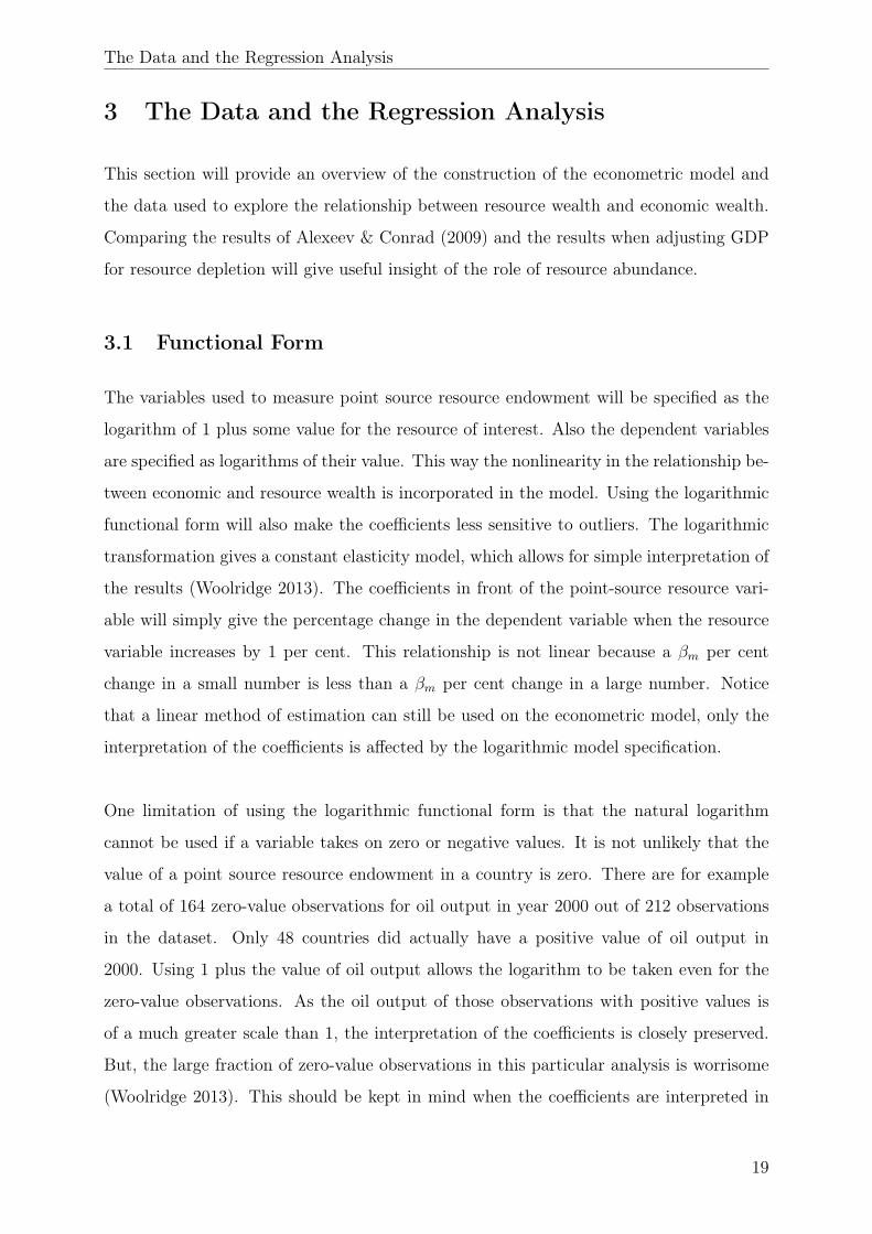
3 The Data and the Regression Analysis
This section will provide an overview of the construction of the econometric model and
the data used to explore the relationship between resource wealth and economic wealth.
Comparing the results of Alexeev & Conrad (2009) and the results when adjusting GDP
for resource depletion will give useful insight of the role of resource abundance.
3.1 Functional Form
The variables used to measure point source resource endowment will be specified as the
logarithm of 1 plus some value for the resource of interest. Also the dependent variables
are specified as logarithms of their value. This way the nonlinearity in the relationship be-
tween economic and resource wealth is incorporated in the model. Using the logarithmic
functional form will also make the coefficients less sensitive to outliers. The logarithmic
transformation gives a constant elasticity model, which allows for simple interpretation of
the results (Woolridge 2013). The coefficients in front of the point-source resource vari-
able will simply give the percentage change in the dependent variable when the resource
variable increases by 1 per cent. This relationship is not linear because a βm per cent
change in a small number is less than a βm per cent change in a large number. Notice
that a linear method of estimation can still be used on the econometric model, only the
interpretation of the coefficients is affected by the logarithmic model specification.
One limitation of using the logarithmic functional form is that the natural logarithm
cannot be used if a variable takes on zero or negative values. It is not unlikely that the
value of a point source resource endowment in a country is zero. There are for example
a total of 164 zero-value observations for oil output in year 2000 out of 212 observations
in the dataset. Only 48 countries did actually have a positive value of oil output in
2000. Using 1 plus the value of oil output allows the logarithm to be taken even for the
zero-value observations. As the oil output of those observations with positive values is
of a much greater scale than 1, the interpretation of the coefficients is closely preserved.
But, the large fraction of zero-value observations in this particular analysis is worrisome
(Woolridge 2013). This should be kept in mind when the coefficients are interpreted in
19

The Data and the Regression Analysis
section 4.
3.2 Descriptive Statistics
The analysis will be conducted in the tradition of Alexeev & Conrad (2009). Income-
level regressions are used to test whether oil and mineral endowments are associated with
high levels of economic wealth. Table 1 provides descriptive statistics of the variables.
GDPPC and (GDP-R)PC represents the two dependent variables that will be compared,
while the rest are used as regressors. The information in the table will be of interest when
interpreting the results in the section 4.
Table 1: Descriptive statistics of the variablesVariable Obs. Mean Stand. deviation Min Max
GDPPC 157 8.151 1.168 5.380 10.254(GDP-R)PC 149 1.1576 1.186 -1.318 3.336Hydrocarb. depositsPC 115 0.754 4.603 -4.605 10.595Value of oil outputPC 159 1.779 2.916 0 9.472Oil/GDP ratio 159 0.058 0.167 0 0.961Mining outputPC 118 3.597 2.572 0 8.379Mining/GDP ratio 129 0.053 0.078 0 0.425Absolute latitude 136 22.401 15.727 0.228 63.892European population 138 0.167 0.374 0 1Latin Am. country 138 0.210 0.409 0 1East Asian country 138 0.116 0.321 0 1Ethnic fractionalization 162 0.377 0.289 0 1English speaking frac. 132 0.095 0.269 0 1WestEuro speaking frac. 132 0.299 0.289 0 1.004Settler mortality 82 4.644 1.199 2.146 7.986
3.2.1 Recreating the Analysis of Alexeev & Conrad (2009)
The regression function used by Alexeev & Conrad (2009) takes the form:
GDPPC = β0 +∑
βjX + γN + ε, (6)
20

The Data and the Regression Analysis
In this model ε is the idiosyncratic error term and GDPPC represents the logarithm of
per capita GDP adjusted for purchasing power parity (PPP) in time t=2000. The PPP
GDP data is collected from Maddison (2006). As previously discussed, Alexeev & Conrad
(2009) use the level of GDP, simply because if country A has a higher income level than
country B, then country A must have had a faster long term growth than country B. This
is contrary to Sachs & Warner (1995), who uses the GDP growth rate over a relatively
short period of time.
X is a matrix of control variables. Alexeev & Conrad (2009) use two different approaches
of regressors, one not instrumented and one instrumented. The first approach only con-
sists of clearly exogenous control variables: "Absolute value of latitude" and dummy
variables for "European population", "Latin American country" and "East Asian coun-
try". The instrumented approach includes institutional quality and the degree of ethnic
fractionalization in addition to the dummy variables. The institutional quality is mea-
sured though instruments for rule of law. These are "the fraction of the English-speaking
population", "the fraction of the population speaking a major West European language",
and "the absolute latitude". Also a second set of instruments are estimated, "settler mor-
tality" and "absolute latitude". It can be seen from table 1 that data on settler morality
only exists for 82 observations. As this instrument is unavailable for several countries,
in particular some major oil producers, the sample size is dramatically lowered in the
estimations where settler mortality is included. This means that these estimations are
conducted on less information than the previous ones. However, they are still useful to
study, as this approach to instrumenting rule of law has been used in several previous
studies (e.g. Acemoglu, Johnson & Robinson 2001).
The regressor of particular interest is N, which is a measure of point source resource
endowment. Several measurements for the two point source resources oil and mineral
wealth are used. The first measurement for oil wealth is the logarithm of 1993 hydro-
carbon deposits per capita, with data obtained from Sala-i-Martin, Doppelhofer & Miller
(2004). The second measurement is the logarithm of 1 plus the country‘s per capita pro-
duction of oil in year 2000 at world market prices, with data from BP Statistical Review
21

The Data and the Regression Analysis
(2005) (Alexeev & Conrad 2009). The third measurement is included to accommodate
Sachs & Warner’s (1995) statement that the importance of natural resources in the whole
economy is of interest rather then just endowment per capita. The measurement consists
of the logarithm of 1 plus the ratio of average value of oil output in year 2000 to PPP
GDP. Similarly to the last two measurements for oil wealth, the measurements for mineral
wealth is the logarithm of 1 plus per capita mining output, and the logarithm of 1 plus
the ratio of mining to GDP PPP.
3.2.2 Adjusting GDP for Depletion of Natural Resources
The only addition to Alexeev & Conrad (2009) in this analysis will be the deduction of
natural resource depletion in the dependent variable. By doing so the national income is
adjusted for the value of the resource that is depleted. When a country extracts oil from
the ground, sells it at market price, and receives the income, the transaction in reality
adds up to zero because of the depletion of the oil from the ground. Here it is assumed
that the value of the depletion of natural resources corresponds to rent received for natural
resources. This is a questionable assumption as there obviously will exists more negative
externalities than taken into account by the market. The true social value of resource
depletion is practically impossible to measure, and resource rent will therefore be used for
simplicity. R denotes total resource rent.
Deducting the total natural resource rent from GDP PPP gives a new dependent vari-
able, denoted as GDP-R, which is a more diversified measurement of economic wealth
than GDP alone. The data on total natural resource rent is a part of the primary World
Bank time series on development indicators, compiled from officially recognized interna-
tional sources (The World Bank 2011). The variable of interest is defined as the sum of
oil rents, natural gas rents, coal rents (hard and soft), mineral rents, and forest rents (The
World Bank 2011). The data for resource rent is given as percentage of GDP, denoted
below by r%. It is therefore necessary to transform the data to level values of total natu-
ral resource rents before deducting the value from GDP. This is done by multiplying per
capita GDP in year 2000 from Maddison (2006) by the World Development Indicator of
total natural resource rent as percentage of GDP, and divide by 100. RPC can now be
deducted from GDPPC . In addition, the measurement must be modified to per capita
22

The Data and the Regression Analysis
and natural logarithm specification. The data for year 2000 is used for all the variables
GDP, resource rent and population. The procedure is shown below. Notice the small
letters indicating true levels for the variables, while capital letters indicates logarithmic
values.
• Generate resource adjusted GDP: gdp− r = gdp− gdp×r%100
• Generate per capita GDP-R: (gdp− r)PC = gdp−rpopulation
• Take the natural logarithm: (GDP −R)PC = ln[(gdp− r)PC ]
The new income-level econometric model is specified as:
(GDP −R)PC = β0 +∑
βsX + δN + ε (7)
Using the same methods of estimation on model (6) and model (7) will enable comparison
of the impact of point source resource wealth on the two measures of economic wealth:
Per capita GDP and per capita GDP adjusted for resource depletion. In terms of the two
models, the comparison will be of the economic significance of the γ‘s and the δ‘s.
3.3 The Methods of Estimation
Through a regression analysis the relationship between two or more variables is esti-
mated using a statistical method. In this particular analysis the relationship between
economic wealth and point source resource wealth is of interest. The regressions are run
by ordinary least squares (OLS) estimation and by instrumented variable two stage least
squares (IV 2SLS) estimation. OLS estimation minimizes the sum of squared residuals
(Woolridge 2013). The residuals are the difference between the actual value and the fitted,
or predicted, value for the dependent variable given its regressors. Squaring and summing
all the vertical distances from an observation to the regression line will give best linear
unbiased estimates (BLUE), given the Gauss-Markov assumptions (Woolridge 2013). The
assumptions states that the population model is linear in its parameters, the sample is
random, that there are no perfect linear relationships among the regressors and that the
23

The Data and the Regression Analysis
expected value of the error term is zero and has the same variance given any value of
the regressors. Given all this, there is no other statistical method of estimation that will
give unbiased and linear estimates with smaller variance than the OLS-estimators. In
appendix A these assumptions are listed and the proof for the Gauss-Markov theorem is
provided together with a derivation of the OLS estimates.
The assumption of zero mean in the error term is questionable with regard to the anal-
ysis at hand. If the covariance between an explanatory variable and the error term is
non-zero, then the expected value of the error term given the value of the explanatory
variable is non-zero as well. This is called an endogeneity problem, and if this exists the
OLS estimators will be biased and inefficient (Leighton 2004). Due to the possibility of
an endogeneity problem, regressions are also run with an instrumented variable two stage
least squares estimation. Several authors have pointed out that the institutional quality
might very well be correlated with both economic and natural resource wealth. In this
case there is a simultaneity problem. Due to this, the OLS estimations do not include an
institutional variable. The problem then arises because the effect of institutional quality
will be represented in the idiosyncratic error. When there is a correlation between the er-
ror term and an included regressor, the result will be biased estimates (Woolridge 2013).
The problem is solved through IV 2SLS estimation where one or more instruments is
used to capture the effect of institutional quality on economic wealth and not on resource
endowment. This means that the instruments must satisfy two conditions to be valid.
First, the instrument must be exogenous, meaning it must be uncorrelated with the id-
iosyncratic error term. Secondly, the instrument must be relevant. The instrument is
relevant if there is sufficient empirical correlation between the endogenous variable and
the instrument. If this correlation is weak, called weak identification, the IV estimation
will be less precise than OLS estimation (Woolridge 2013). A test of weak identification
therefore should, and will be, conducted.
The IV 2SLS estimator can be obtained in two stages, hence the name. In the first
step a reduced form model is estimated by normal OLS (Verbeek 2013). The reduced
form model is the endogenous regressor from the original model, from now called the
structural model, as left hand side variable and the instruments and the exogenous vari-
24

The Data and the Regression Analysis
ables from the structural model as regressors. In the second stage the predicted values
from the reduced form replaces the endogenous regressor in the structural model. OLS is
now used to regress the dependent variable on the instrumented variable. In the case of
using the rule of law index for institutional quality, and fraction of the English-speaking
population, fraction of the population speaking a major West European language and
absolute latitude as instrument, the procedure is preformed as follows:
Step 1: Compute the OLS regression of "Rule of law" on all the instruments and
the exogenous variables (represented by the X matrix) from the structural model. µ
represents the error term from the reduced form regression.
Rule of law = γ1(English speaking frac.) + γ2(WestEuro speaking frac.)
+ γ3(Absolute latitude) +∑
βmX + µ(8)
Step 2: Use OLS to regress the structural model with the instrumental variable, "Rule
of law", included:
GDP = βIV0 + β1N + β2Rule of law +∑
βmX + ε (9)
The result will give the IV estimates:
GDP = ˆβIV0 + β1N + ˆβIV2 Rule of law +∑
ˆβIVm X (10)
Notice that the hats indicate predicted values and that IV denotes the instrumented
variable estimates. The two regression methods presented, OLS and IV 2SLS, are the
ones that will be used to study the relationship between resource and economic wealth.
All regressions in this analysis is run in the software package STATA, and all the estimated
coefficients are presented in Appendix C.
25

The Data and the Regression Analysis
3.4 Inferential Statistics
The similar structure of the OLS and the IV 2SLS estimators gives similar statistical
inference for the two methods of regression. Statistical inference allows deduction about
the population model from the random sample described by the descriptive statistics
(Woolridge 2013). To preform inference on the coefficients, an additional assumption
must be made to the Gauss-Markov assumptions. The distribution of the coefficients
depends on the underlying distribution of the errors. Assuming the errors to be normally
distributed, together with the zero conditional mean and homoscedasticity condition, is
formally expressed as:
ε ∼ Normal(0, σ2),
whith σ2 being the constant variance for any given value of the regressors. In the case
of instrumented variables, the homoscedasticity assumption is stated conditional on the
instrumental variable, and not the endogenous instrumented variable. Under these as-
sumptions it can be shown that a coefficient βm is normally distributed with the expected
value βm and variance var(βm) where βm is the true population coefficient and βm is the
estimated coefficient (Woolridge 2013). This implies that:
βm−βmsd(βj)
∼ Normal(0, 1),
where sd(βm) is the standard deviation of the coefficient. This result is used to con-
struct test statistics. The estimated standard deviation is called the standard error, and
denoted as se(βm).
3.4.1 Testing the Estimates
The estimated coefficients will give the marginal effect of its corresponding variable on the
dependent variable. In order to prove the statistical significance of the coefficients they
must be tested. Given the assumptions made above, the test statistic, tdf , is student-t
26
The Data and the Regression Analysis
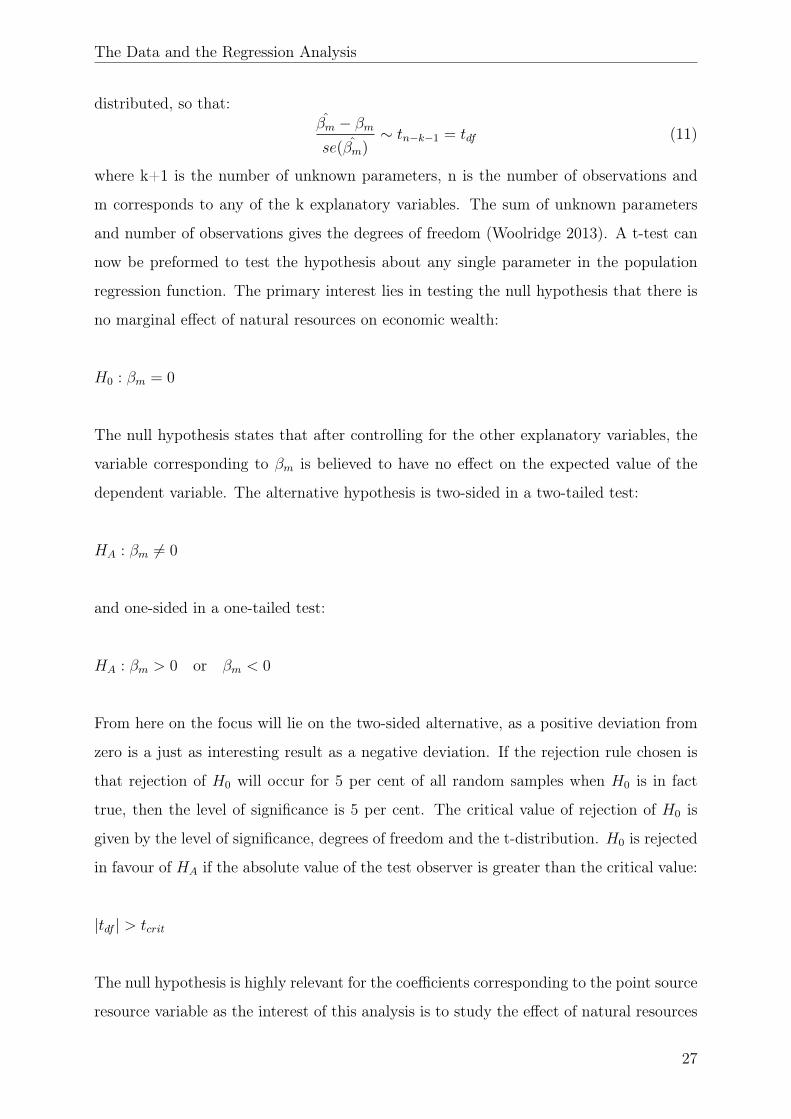
distributed, so that:βm − βmse(βm)
∼ tn−k−1 = tdf (11)
where k+1 is the number of unknown parameters, n is the number of observations and
m corresponds to any of the k explanatory variables. The sum of unknown parameters
and number of observations gives the degrees of freedom (Woolridge 2013). A t-test can
now be preformed to test the hypothesis about any single parameter in the population
regression function. The primary interest lies in testing the null hypothesis that there is
no marginal effect of natural resources on economic wealth:
H0 : βm = 0
The null hypothesis states that after controlling for the other explanatory variables, the
variable corresponding to βm is believed to have no effect on the expected value of the
dependent variable. The alternative hypothesis is two-sided in a two-tailed test:
HA : βm 6= 0
and one-sided in a one-tailed test:
HA : βm > 0 or βm < 0
From here on the focus will lie on the two-sided alternative, as a positive deviation from
zero is a just as interesting result as a negative deviation. If the rejection rule chosen is
that rejection of H0 will occur for 5 per cent of all random samples when H0 is in fact
true, then the level of significance is 5 per cent. The critical value of rejection of H0 is
given by the level of significance, degrees of freedom and the t-distribution. H0 is rejected
in favour of HA if the absolute value of the test observer is greater than the critical value:
|tdf | > tcrit
The null hypothesis is highly relevant for the coefficients corresponding to the point source
resource variable as the interest of this analysis is to study the effect of natural resources
27
The Data and the Regression Analysis
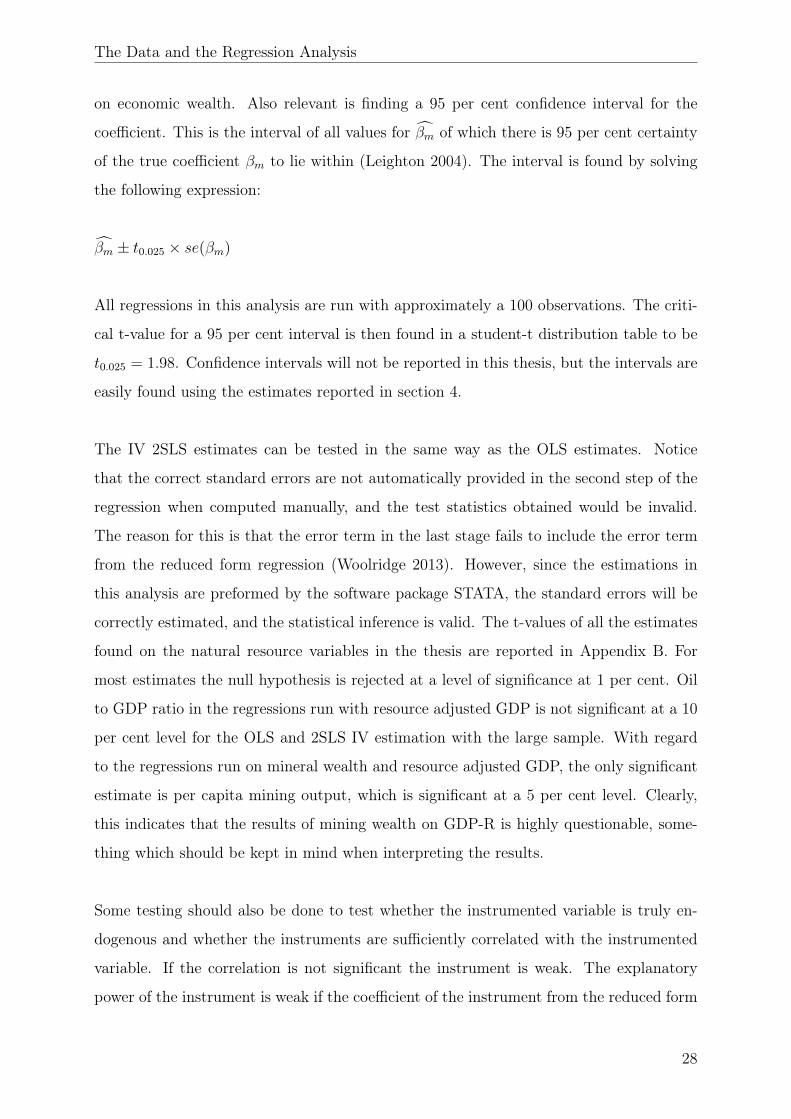
on economic wealth. Also relevant is finding a 95 per cent confidence interval for the
coefficient. This is the interval of all values for βm of which there is 95 per cent certainty
of the true coefficient βm to lie within (Leighton 2004). The interval is found by solving
the following expression:
βm ± t0.025 × se(βm)
All regressions in this analysis are run with approximately a 100 observations. The criti-
cal t-value for a 95 per cent interval is then found in a student-t distribution table to be
t0.025 = 1.98. Confidence intervals will not be reported in this thesis, but the intervals are
easily found using the estimates reported in section 4.
The IV 2SLS estimates can be tested in the same way as the OLS estimates. Notice
that the correct standard errors are not automatically provided in the second step of the
regression when computed manually, and the test statistics obtained would be invalid.
The reason for this is that the error term in the last stage fails to include the error term
from the reduced form regression (Woolridge 2013). However, since the estimations in
this analysis are preformed by the software package STATA, the standard errors will be
correctly estimated, and the statistical inference is valid. The t-values of all the estimates
found on the natural resource variables in the thesis are reported in Appendix B. For
most estimates the null hypothesis is rejected at a level of significance at 1 per cent. Oil
to GDP ratio in the regressions run with resource adjusted GDP is not significant at a 10
per cent level for the OLS and 2SLS IV estimation with the large sample. With regard
to the regressions run on mineral wealth and resource adjusted GDP, the only significant
estimate is per capita mining output, which is significant at a 5 per cent level. Clearly,
this indicates that the results of mining wealth on GDP-R is highly questionable, some-
thing which should be kept in mind when interpreting the results.
Some testing should also be done to test whether the instrumented variable is truly en-
dogenous and whether the instruments are sufficiently correlated with the instrumented
variable. If the correlation is not significant the instrument is weak. The explanatory
power of the instrument is weak if the coefficient of the instrument from the reduced form
28

The Data and the Regression Analysis
regression is insignificant (Verbeek 2013). The software package STATA reports the value
of the F-statistic, which is a measure of the information content contained in the instru-
ments. A simple rule-of-thumb says that one need not worry about weak instruments if
the F-statistic exceeds 10. All F-statistics from the regression of economic wealth in this
thesis exceeds the rule-of-thumb, and are reported in Appendix B.
If the instrumented variable is not endogenous the IV 2SLS estimator is less efficient,
meaning it has a larger standard error, than the OLS estimator (Woolridge 2013). Endo-
geneity can be tested using a Hausman test. First, the reduced form model is estimated
and the residuals µ is obtained. Adding µ to the structural equation, without substituting
the instrumented variable, will now allow testing for the significance of µ. This procedure
is illustrated in equation 12.
GDPOLS = ˆβOLS0 + ˆβOLS1 N + ˆβOLS2Rule of law + βX + ˆθOLSµ (12)
Regressing equation 12 by OLS will provide a coefficient for µ, ˆθOLS, which can be tested
using a simple t-test with H0 : θ = 0. In equation 9, it is assumed that each instrument is
uncorrelated with ε. The instrument "Rule of law" is therefore exogenous only if µ is un-
correlated with ε, which will only occur if H0 is true. If ˆθOLS is statistically different from
zero it can be concluded that "Rule of law" is indeed endogenous. In this case "Rule of
law" is not a valid instrument. In Appendix B the results of Husman testing is provided.
Through the software package STATA the test can be run without estimating the reduced
form equation. Here, the null hypothesis is that the instrument is exogenous, and under
this hypothesis the test statistic is chi-squared distributed with the number of degrees of
freedom equal to the number of regressors being tested for endogeneity. H0 is rejected
if the test statistic exceeds the critical chi-squared value at a chosen level of significance
(Baum, Schaffer & Stillman 2003). When H0 is rejected here, there is an endogeneity
problem because the instrument does not fulfil the exogeneity condition. Unfortunately,
the test results in Appendix B indicate that several of the regressions suffers from this
problem. This advocates the use of OLS estimation to 2SLS IV in these regressions.
An IV model is exactly identified if the number of instruments equals the number of
endogenous regressors, and overidentified if the number of instruments exceeds the num-
29

The Data and the Regression Analysis
ber of endogenous regressors (Verbeek 2013). The analysis conducted here uses two dif-
ferent sets of instruments, both containing more instruments than the one endogenous
variable "institutional quality". This gives overidentified models, and an overidentifying
restrictions test, also called a Sargan test, should be conducted (Verbeek 2013). With
the typical sample size available severe biases in the IV 2SLS estimates can be created
when too many instruments are added. Through a Sargan test it is found whether any
of the instruments correlates with the structural error term. The null hypothesis is that
the model is correctly overidentified. This is tested by estimating the structural equation
by IV 2SLS and obtaining the residuals ε. Then the estimated residuals are regressed on
all exogenous variables and the R-squared from this regression is obtained: R21. Under
the null hypothesis it is true that the Sargan statistic is asymptotically chi-squared dis-
tributed:
nR21 ∼ χ2
q,
where q is the number of instruments minus the number of endogenous regressors, and n
is the number of observations (Verbeek 2013). If the statistic exceeds the critical value
chosen in the chi-squared distribution the null hypothesis is rejected. This could mean
that the model is misspecified because an instrument is correlated with the error, or that
an instrument is omitted as a variable in the model. The set of instruments should then
be revisited because at least one of the instruments is invalid. The Sargan statistics are
reported in Appendix B. They conclude that in all regressions the null hypothesis cannot
be rejected, indicating that the overidentifying restrictions in the model is correct.
3.5 The Hypothesis
Being provided with the very same data used in Alexeev & Conrad’s (2009) analysis,
the results of this regression will be of interest in two main aspects. First, is the effect
of natural resources on economic wealth affected by depletion of natural resources? The
expected answer is of course yes. As GDP alone does not include the pre-extraction value
of resource endowment the effect of resource endowment on economic wealth is likely to
be too large when regressing upon GDP. It is highly reasonable that the positive effect of
30
The Data and the Regression Analysis
resources on economic wealth is less prominent when resource depletion is adjusted for.
Secondly, is the resources curse hypothesis still rejected when correcting the regression
for resource depletion? The expectations are not so clear for this question. Earlier it
was discussed that there are reasons to believe that Alexeev & Conrad (2009) analysis is
positively biased due to endogeny problems in the explanatory variable of interest. This
problem would still occur in the current analysis. The negative bias in Sachs & Warner
(1995) due to the short time period in the GDP growth rate used as dependent variable
is corrected by using levels rather than growth. With the expected negative effect of
correcting GDP for resource depletion and the positive effect of using levels rather than
growth proven by Alexeev & Conrad (2009), it is reasonable to believe that the regression
at hand will be some sort of a compromise between the analysis of Sachs & Warner (1995)
and Alexeev & Conrad (2009). But only a negative impact of natural resource wealth on
economic wealth can underpin the prediction of a resource curse.
The hypothesis is supported by the results presented in the next section. Including re-
source depletion gives lower estimated effect of natural resources on economic wealth.
The effect is, however, still shown to be positive, which suggests that the resource curse
should, in its simplest form, be rejected. As was briefly discussed earlier, there may still be
reasons to believe that this conclusion may be changed if one were to find true exogenous
vacation in the measure of resource wealth. Also, there may exist a conditional resource
curse, meaning that the resource curse only occurs under certain conditions. This topic
will be further elaborated on in section 5.
31

Presentation and Interpretation of the Results
4 Presentation and Interpretation of the Results
This section will compare the results of Alexeev & Conrad (2009) to the results of the
the same analysis when adjusting for resource depletion. First the effects of oil wealth
are presented, and next the effects of mineral wealth. Running the regressions described
in the previous section provide the results expected: The effect of point source resource
wealth on economic wealth is a compromise between Alexeev & Conrad (2009) and Sachs
& Warner (1995) when GDP is adjusted for resource depletion. The results are presented
in tables 2 to 7, together with the results of Alexeev & Conrad (2009), so that they can
easily be compared. The regressions on oil wealth are presented in tables 2, 3 and 4, while
regressions on mining wealth are presented in tables 5, 6 and 7. For simplicity, only the
coefficients of the variables measuring the point source resource are presented together
with the robust standard errors in parenthesis. A full presentation of the results can be
found in Appendix C.
4.1 The Effect of Oil Wealth
The results of Alexeev & Conrad (2009) are indisputable: Countries rich in oil tend to
have relatively high levels of GDP. The estimates of the impact of oil endowment are all
positive and highly statistically significant. The estimates vary between 0.26 and 2.57,
and are therefore also economically significant. Remember that the dependent variable is
specified in natural logarithm and so are all the variables measuring resource endowment.
The results must therefore be interpreted as elasticities (Woolridge 2013). From table
2, the coefficient in front of the variable "per capita hydrocarbon deposits" equals 0.059
with a robust standard error at 0.016. All else equal, the coefficient is interpreted as
the elasticity between per capita GDP and hydrocarbon deposits. This is easily seen by
taking the partial derivative from the regression:
ln(GDPPC9 = 6.712 + 0.059ln(Hydro.depPC) + 0.037abs.latitude
+1.340euro.pop+ 1.018latin.am+ 1.703east.asia,(13)
32

Presentation and Interpretation of the Results
which will wield:
1
GDPPC× ∂GDPPC = 0.059× 1
Hydro.depPC× ∂Hydro.depPC (14)
The elasticity is now found as:
∂GDPPC × 100
GDPPC= 0.059× ∂Hydro.depPC × 100
Hydro.depPC(15)
⇒ %∆GDPPC = %∆Hydro.depPC × 0.059 (16)
Table 2: OLS estimation - Effect of Oil Wealth on Economic WealthLine Explanatory variable Dependent variable Coefficient
1 Hydrocarb. depositsPC GDPPC 0.059(0.016)
2 Hydrocarb. depositsPC (GDP-R)PC 0.041(0.015)
3 Value of oil outputPC GDPPC 0.096(0.023)
4 Value of oil outputPC (GDP-R)PC 0.054(0.023)
5 Oil/GDP ratio GDPPC 1.507(0.693)
6 Oil/GDP ratio (GDP-R)PC 0.793(0.714)
The elasticity is constant throughout, meaning that a 1 per cent increase in the per capita
hydrocarbon deposits on average, all else equal, will increase the per capita GDP by 0.059
per cent. What this essentially means is that the function form is assumed to have the
following quality: When hydrocarbon deposits increases towards infinity, the marginal
impact of a change in hydrocarbon deposits on GDP levels goes towards zero. In other
words, the impact of hydrocarbon deposits on GDP levels are always positive, but in a
decreasing manner.
33

Presentation and Interpretation of the Results
Table 3: IV 2SLS estimation - Effect of Oil Wealth on Economic WealthLine Explanatory variable Dependent variable Coefficient
1 Hydrocarb. depositsPC GDPPC 0.051(0.010)
2 Hydrocarb. depositsPC (GDP-R)PC 0.025(0.010)
3 Value of oil outputPC GDPPC 0.086(0.015)
4 Value of oil outputPC (GDP-R)PC 0.036(0.016)
5 Oil/GDP ratio GDPPC 1.255(0.313)
6 Oil/GDP ratio (GDP-R)PC -0.002(0.344)
Comparing the effect of hydrocarbon deposits on GDP to the effect of hydrocarbon de-
posits on resource rent corrected GDP, yields the results expected. The two first lines in
table 2 shows a less positive impact of per capita hydrocarbon deposits on GDP - R than
on GDP alone. The coefficient of 0.059 with a t-value of 3.79 is statistically significant
even at a 1 per cent significance level. Interpretation of this coefficient yields that a 1
per cent increase in per capita hydrocarbon deposits would yield 0.059 per cent increase
in GDP per capita. The difference in impact predicted by Alexeev & Conrad (2009) is
substantially larger than the impact on economic wealth when resource depletion is ac-
counted for. A 1 per cent increase in hydrocarbon deposits only yields a 0.041 per cent
increase in the adjusted dependent variable.
The mean of the variable GDP is found to be 8.239. From the two last lines in table
2 it is seen that a 1 per cent increase in Oil/GDP ratio is predicted to increase GDP by
1.507 per cent. For the mean value country, this would imply an increase in PPP GDP
per capita of 0.12 units:1.507× 8.239
100= 0.12 (17)
34

Presentation and Interpretation of the Results
The same increase in Oil/GDP ratio is predicted to increase adjusted measure, GDP - R,
by 0.793 per cent. Since the mean per capita GDP - R equals 1.1576, the effect would be
0.01 units:
0.793× 1.1576
100= 0.01 (18)
As expected, the impact is less economically significant when depletion of natural re-
sources is taken into account. In this case however, as will be shown to also be true for
the larger fraction of the other regressions preformed in this thesis, the resource curse is
still not rejected when economic wealth is measured as GDP minus resource rent. The
results from the regressions using the per capita value of oil output as regressor shows
that the elasticity on per capita GDP is 0.096, while it is 0.054 for the same measure
corrected for resource rents. All results in table 2 is statistically significant at a 1 per cent
significance level.
In the previous section it was argued why a IV 2SLS estimation is also included. The
results are presented in table 3. Note that the measures for oil endowment are the same
as in table 2, however the remaining regressors are not identical. The details can be found
in Appendix C. The trend in table 3 shows the same as table 2: When deducting resource
rent from GDP the positive effect of oil endowment on economic wealth is reduced. Only
the last estimation, where the share of oil to GDP is regressed upon GDP adjusted for
resource depletion, gives a slightly negative coefficient. This effect is not significant even
at a 10 per cent significance level, and therefore not further discussed. The other effects
on the adjusted GDP variable is significant at a 5 per cent significance level, while the
effects from Alexeev & Conrad’s (2009) estimations are all significant at a 1 per cent level.
All the reported F-statistics on weak identification is above 10, and weak instruments is
therefore not a problem here according to the rule-of-thumb.
Table 4 uses the same method of estimation as table 3, only with other instruments.
As settler mortality is unavailable for many of the observations the sample size in these
regressions are substantially smaller. But still, the results for table 4 shows the same
trend as the tables above. When GDP is corrected for depletion of natural resources the
coefficients are less positive. Alexeev & Conrad’s (2009) estimates are significant at a 1
35

Presentation and Interpretation of the Results
Table 4: Effect of Oil Wealth on Economic Wealth - smaller sample
Line Explanatory variable Dependent variable Coefficient
1 Hydrocarb. depositsPC GDPPC 0.064(0.013)
2 Hydrocarb. depositsPC (GDP-R)PC 0.038(0.012)
3 Value of oil outputPC GDPPC 0.131(0.018)
4 Value of oil outputPC (GDP-R)PC 0.079(0.019)
5 Oil/GDP ratio GDPPC 2.567(0.712)
6 Oil/GDP ratio (GDP-R)PC 0.993(0.574)
per cent level. The effect of hydrocarbon deposits and the value of oil output on adjusted
GDP is significant at a 1 per cent significance level, while the effect of the oil to GDP
ratio, in the last line of table 4, only is significant at a 10 per cent level. Also here all
reported F-statistics indicates that there is no problem of weak instruments.
4.2 The Effect of Mineral Wealth
The results of the regressions run with mineral wealth as regressor is presented in tables
5, 6 and 7. Also these regressions have a log-log function form, and the coefficients can be
interpreted as elasticities. As an example, the first two lines in table 5 shows that a 1 per
cent increase in per capita mining output will increase per capita GDP by 0.094 per cent,
but per capita GDP adjusted for resource depletion will only be increased by 0.061 per
cent. Using the same exercise used earlier for the hydrocarbon deposits, it is now found
that a 1 per cent increase in the share of mining to GDP will increase per capita GDP by
0.21 units:2.603× 8.239
100= 0.21 (19)
36

Presentation and Interpretation of the Results
The same increase in mining to GDP ratio will only increase per capita GDP adjusted
for resource depletion by 0.02 units:
1.618× 1.1576
100= 0.02 (20)
Un this particular regression, the difference in the marginal effect of point source resource
endowment is of 1.9 percentage points.
Table 5: OLS estimation - Effect of Mineral Wealth on Economic WealthLine Explanatory variable Dependent variable Coefficient
1 Mining outputPC GDPPC 0.094(0.028)
2 Mining outputPC (GDP-R)PC 0.061(0.027)
3 Mining/GDP ratio GDPPC 2.603(1.111)
4 Mining/GDP ratio (GDP-R)PC 1.618(1.040)
The same trend is seen when using IV estimation in tables 6 and 7. Mining to GDP ratio
positively effects GDP with a coefficient on 1.444 in the fourth line of table 6. When
resource rents are deducted the same coefficient becomes slightly negative. However, the
coefficient is only statistically significant at a 10 per cent level. The effect of the value
of mining output, showed in the second line, is not statistically significant even at a 10
per cent significance level. In table 7 the smaller sample size regressions give the same
trends. Unfortunately the results of the effect on adjusted GDP is not very robust since
none of the variables for mining wealth are statistically significant even at a 10 per cent
significance level. The overall results however underpins the results from the analysis on
oil endowment: When adjusting GDP for resource rents the effect of mineral wealth is
reduced.
Based on the estimation results of oil and mineral endowment on economic wealth, it can
be stated that the positive effect of resource endowment on economic wealth is reduced
37

Presentation and Interpretation of the Results
Table 6: IV 2SLS estimation - Effect of Mineral Wealth on Economic WealthLine Explanatory variable Dependent variable Coefficient
1 Mining outputPC GDPPC 0.062(0.020)
2 Mining outputPC (GDP-R)PC 0.025(0.019)
3 Mining/GDP ratio GDPPC 1.444(0.846)
4 Mining/GDP ratio (GDP-R)PC -0.488(0.721)
Table 7: Effect of Mineral Wealth on Economic Wealth - smaller sample
Line Explanatory variable Dependent variable Coefficient
1 Mining outputPC GDPPC 0.082(0.029)
2 Mining outputPC (GDP-R)PC 0.036(0.027)
3 Mining/GDP ratio GDPPC 4.506(1.372)
4 Mining/GDP ratio (GDP-R)PC 1.621(1.327)
when depletion of resources is taken into account. The results also suggests that adjusting
GDP for resource depletion does not change the conclusion of Alexeev & Conrad (2009).
The prediction of a resource curse seems to be false, or at the very least can not be verified.
Even when adding the depletion of natural resources, the effect of being rich in point
source resources seems to have a positive effect on economic wealth. These conclusions
may however change if only a conditional resource curse is what is hypotezised. What if
countries with some characteristics suffers from the resource curse, while others do not?
So far the resource curse has been studied in its simplest form. The next section will
assess the conditional resource curse prediction.
38

The Conditional Resource Curse Prediction
5 The Conditional Resource Curse Prediction
The analysis thus far has not been able to confirm the existence of a resource curse
in the sense that, all else equal, countries rich in resources are to be less economically
wealthy. But, as was shown in figure 1, the fact that some countries rich in resources
tend to preform poorly in economical terms cannot be disputed. One of the interesting
aspects of this topic is the huge variation in the economic performance of resource-rich
nations. In this section different dimensions in which "cursed" and "non-cursed" resource-
rich countries differ, are identified to examine possible variables that the curse could be
conditional upon. The hypothesis of a resource curse conditional upon institutional quality
is commonly used. Some theory on this topic will be presented here, and an analysis in
the tradition of Alexeev & Conrad (2009) is then conducted. Like in the previous sections,
the measurement for economic wealth will be expanded to include resource depletion.
5.1 What could the Resource Curse be Conditional Upon?
In Torvik’s (2009) search for dimensions in which resource abundant winners and losers
differ, the following six are identified. The first one is saving of resource income. The
mechanism and intuition of genuine savings, or net adjusted savings, was introduced in
section 2. According to Torvik (2009), there is systematic differences in the resource-
adjusted savings rates between those countries that have escaped the resource curse and
those that have not. However, causality can not be proven. There is a tendency for
those economies that has escaped to have higher genuine savings than those who have
not escaped the curse. But, there is no way of knowing if the degree of saving resource
income affects the economic development, or if poor economic development has resulted in
overspending of resource income. The finding is interesting and underpins the importance
of using diversified indicators when measuring economic wealth. This discussion is closely
related to the analysis conducted later on in this section, where the conditional curse is
tested using resource-adjusted GDP as dependent variable.
A second dimension identified by Torvik (2009) is the type of natural resources in the
economy. Clearly the value of different resources will differ, and therefore the influence on
39
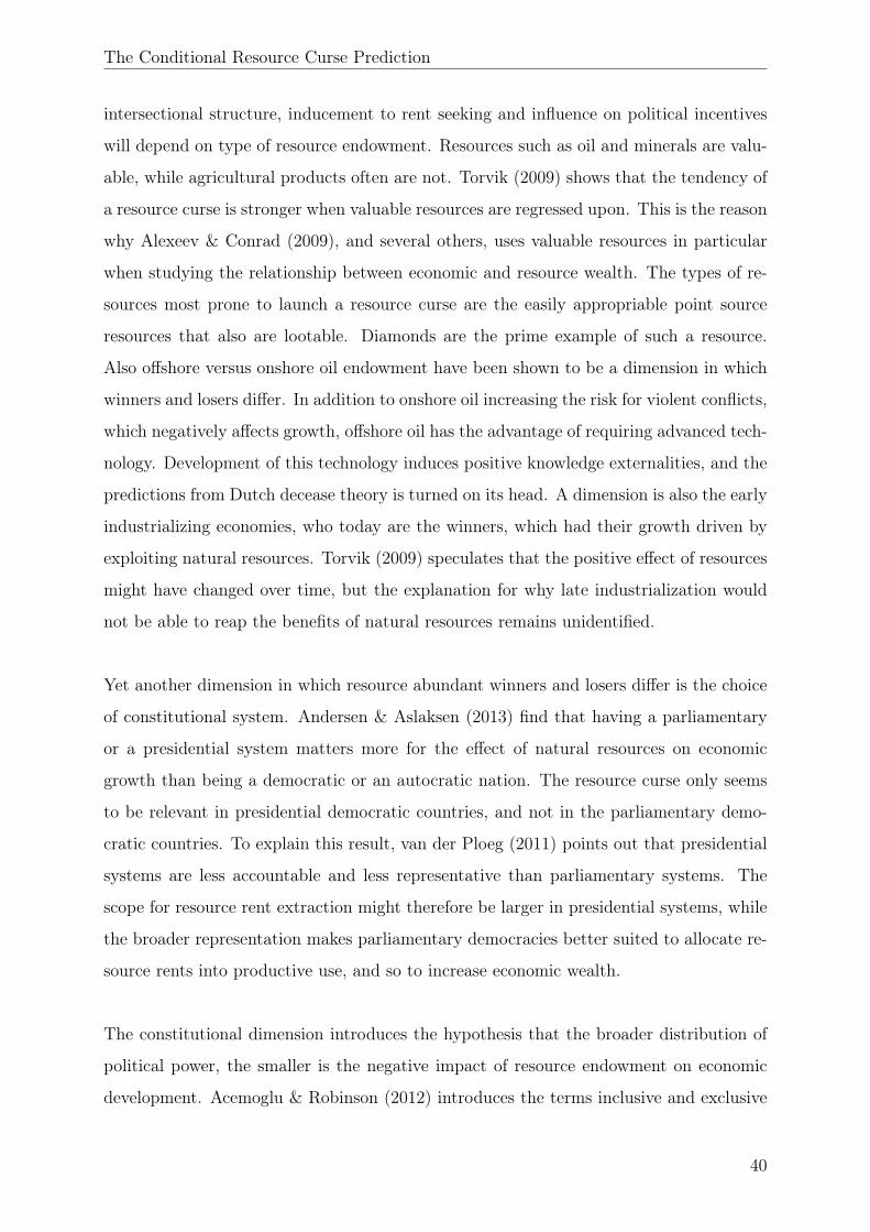
The Conditional Resource Curse Prediction
intersectional structure, inducement to rent seeking and influence on political incentives
will depend on type of resource endowment. Resources such as oil and minerals are valu-
able, while agricultural products often are not. Torvik (2009) shows that the tendency of
a resource curse is stronger when valuable resources are regressed upon. This is the reason
why Alexeev & Conrad (2009), and several others, uses valuable resources in particular
when studying the relationship between economic and resource wealth. The types of re-
sources most prone to launch a resource curse are the easily appropriable point source
resources that also are lootable. Diamonds are the prime example of such a resource.
Also offshore versus onshore oil endowment have been shown to be a dimension in which
winners and losers differ. In addition to onshore oil increasing the risk for violent conflicts,
which negatively affects growth, offshore oil has the advantage of requiring advanced tech-
nology. Development of this technology induces positive knowledge externalities, and the
predictions from Dutch decease theory is turned on its head. A dimension is also the early
industrializing economies, who today are the winners, which had their growth driven by
exploiting natural resources. Torvik (2009) speculates that the positive effect of resources
might have changed over time, but the explanation for why late industrialization would
not be able to reap the benefits of natural resources remains unidentified.
Yet another dimension in which resource abundant winners and losers differ is the choice
of constitutional system. Andersen & Aslaksen (2013) find that having a parliamentary
or a presidential system matters more for the effect of natural resources on economic
growth than being a democratic or an autocratic nation. The resource curse only seems
to be relevant in presidential democratic countries, and not in the parliamentary demo-
cratic countries. To explain this result, van der Ploeg (2011) points out that presidential
systems are less accountable and less representative than parliamentary systems. The
scope for resource rent extraction might therefore be larger in presidential systems, while
the broader representation makes parliamentary democracies better suited to allocate re-
source rents into productive use, and so to increase economic wealth.
The constitutional dimension introduces the hypothesis that the broader distribution of
political power, the smaller is the negative impact of resource endowment on economic
development. Acemoglu & Robinson (2012) introduces the terms inclusive and exclusive
40

The Conditional Resource Curse Prediction
political and economic institutions. The broader the distribution of power, the more in-
clusive are the political institutions. Extractive political institutions on the other hand,
concentrate the power within a small elite, and put few constraints on how the power is
used. Acemoglu & Robinson (2012) go on arguing that there is strong feedback loops the
economic and political institutions, and extractive economic institutions will hinder the
engines of economic growth and development through biased distribution of resources.
In this case, the more resources available, the more will the political elite have to gain
on maintaining a narrow distribution of power. The exclusive economic institutions will
be maintained so that the elite can continue to extract resources. This synergistic rela-
tionship can be broken trough critical junctures, which are stochastic events affecting the
institutional arrangements. Notice that the feedback loops generates a multicollinearity
problem because institutions are endogenously determined by natural resources. This
could cause biased estimates in the regression analysis.
5.2 Institutional Quality as Condition
To some degree many of the dimensions described above are clearly linked to institutional
quality. North (1991) defines institutions as "the humanly devised constraints that struc-
ture political, economic and social interaction". They are rules that describe both what
is allowed to do and also what is actually done, by agents and organizations in a society.
The institutions can be formal, like laws and property rights, or informal, like traditions,
customs or taboos. By providing the incentive structure in the societies they also directs
the economic development towards growth and prosperity, stagnation or even decline.
With this in mind it is safe to state that understanding institutions is important for un-
derstanding the determinants of economic development and wealth. The hypothesis that
the resource curse could be conditional upon institutional quality should be investigated.
At least two questions can be researched with regard to the role of institutions in re-
gressing natural resource wealth upon economic wealth. First, will the amount of natural
resources affect the quality of a nation’s institutions? Secondly, will a nations existing in-
stitutional quality affect the impact of resource endowment on economic prosperity? The
first question is well elaborated in the rent seeking theory. It is believed that resource
41

The Conditional Resource Curse Prediction
abundance deteriorates institutional quality through rent seeking activities, which will
increase the rent seekers wealth without creating additional wealth in the society. The
result is reduced economic efficiency through reduced wealth creation, deteriorated re-
source allocations and potentially reduced economic wealth (Dabla-Norris & Wade 2001).
On the basis that they find at most weak correlation between resource abundance and
institutional quality, Sachs & Warner (1995) dismisses the possibility of resources having
an impact on institutions. This also eliminates the multicollinearity problem discussed
earlier. On the basis on this they dismiss the conditional curse, and uses Dutch disease
explanations to support the negative impact of resources on economic performance.
Mehlum, Moene & Torvik (2006) finds that institutions are decisive for the resource
curse, contradicting Sachs & Warner’s (1995) claims. This relates to the second question.
The hypothesis that poor institutional quality is the cause of the resource curse and that
good enough institutions can eliminate the curse entirely is confirmed by including an in-
teraction term in Sachs & Warner’s (1995) regressions. The regression model is expanded
by the term SXP×IQ, where IQ measures institutional quality. Using the same data as
Sachs & Warner (1995), Mehlum et al. (2006) find the effect of a marginal increase in
SXP on GDP growth to be:
∂(G7089)
∂(SXP )= −14.34 + 15.40(IQ) (21)
The means that the effect of a marginal increase in resource abundance on economic
growth depends on institutional quality. The IQ variable is an unweighted average of five
indexes measuring different aspects of the institutional quality, and the index ranges from
zero to unity 2. An institutional quality value of one would imply perfect institutions,
while zero would imply the poorest possible quality. To escape the resource curse, a coun-
try must have a value of institutional quality exceeding the threshold, IQ0 = 0.93:
−14.34 + 15.40(IQ0) = 0 ⇒ IQ0 = 14.34/15.40 = 0.93.
The above result is explained through a model where entrepreneurs are either grabbers2The index is based on data from Political Risk Services. It consists of a rule of law, bureaucratic
quality, corruption in government, risk of expropriation and government repudiation of contracts index,measured as of 1982.
42

The Conditional Resource Curse Prediction
who appropriate as much possible of the resource rent, or productive producers generating
economic growth. Grabber friendly institutions will induce entrepreneurs to switch from
productive to grabber activities, which lowers growth. Producer friendly institutions on
the other hand, enables a country to take full advantage of its resources, preventing the
negative resource curse effect. The crucial threshold of producer friendly institutions,
derived above, was found to be at 0.93. In the sample of Mehlum et al. (2006) it was
found that the resource curse prediction is not valid for top 20 percent with regard to in-
stitutional quality. This strongly indicates a resource curse conditional upon institutional
quality.
There are some potential problems in the analysis preformed by Mehlum et al. (2006).
Although the effects of secondary school enrollment and ethnic and language fraction-
alization are tested for, a problem of omitted variable bias could still occur. Resource
abundance could be correlated with an excluded measure of underdevelopment. As pre-
viously discussed, the finding of a truly exogenous measurement of resource wealth would
prevent this issue. Mehlum et al. (2006) worries that the empirical results might be driven
by a correlation between underdevelopment and specialization in agricultural exports, for
instance. Land is less lootable and taxable than many other natural resources, and re-
source grabbing might therefore be less likely to occur in countries rich in agricultural
resources. This possible bias is tested by investigating the relationship between GDP
growth and mineral abundance, which is a lootable resource. The direct negative effect
of resources on economic growth increases in this regression. Also the interaction term
increases. This indicates that lootable resources are particularly harmful for growth in
countries with poor institutional quality. The result strengthens the prediction of a con-
ditional curse, as the mechanism through grabber friendly institutions seems to work even
better when only lootable resources are assessed. Without a truly exogenous measure for
resource wealth however, awareness of omitted variable bias must be made.
According to rent seeking theory, the positive effect of natural resources on economic
wealth found by Alexeev & Conrad (2009) is flawed due to the time horizon. With time,
natural resources could deteriorate institutional quality, which would be negative for eco-
nomic development. Alexeev & Conrad (2009) dismisses the conditional resource curse
43

The Conditional Resource Curse Prediction
and argues that oil and minerals are largely neutral with respect to institutional quality.
They believe that studies finding a negative relationship between natural resources and
institutions are flawed due to the inclusion of per capita GDP as a control variable. As
was discussed in section 2, the relationship between resource wealth and GDP is argued
to be flawed because early extraction of resources has influenced the GDP levels of later
periods. Given this positive relationship, and the positive relationship between GDP and
institutions, the estimates of natural resources on institutions are negatively biased. This
is proved through an analysis by Alexeev & Conrad (2009), which will be thoroughly
examined below.
The point, Alexeev & Conrad (2009) argues, is that natural resources does not hurt
institutions, it simply does not improve them either. For now, imagine that it is true that
resources increases GDP, but have no simultaneous effect on institutions in the short and
medium term. Two identical countries are compared with regard to resources, institutions
and economic wealth. As manna from heaven, country 1 becomes rich in oil. The GDP
level increases, but institutional quality remain. The ratio between institutional quality
and GDP is now better for country 2 than for country 1, because the denominator of
country 1 is larger. Institutional quality in country 2, given the GDP level, is relatively
better than for that of country 1. Before country 1 was "blessed" with oil, this ratio was
equal. So, apparently, oil will induce a negative effect on institutional quality. Clearly, the
effect is flawed and only represents the positive effect of natural resources on the initial
GDP level.
Not surprisingly, the results in the previous section show positive coefficients for the
instrument "Rule of law", which means that institutions correlates positively with eco-
nomic wealth. However, Alexeev & Conrad (2009) also finds that countries with weaker
institutions benefits more from natural resources, through a regression where the inter-
action term "Rule of law × Natural Resources", or "IQ × N", is included. Due to the
potential endogeneity between institutions and GDP, the predicted values of IQ are ob-
tained from the first stage in the 2SLS IV regressions described earlier. These are marked
by the subscript p. They are then inserted to the regression function, which now takes
the form:
44

The Conditional Resource Curse Prediction
GDPPC = β0 +∑
βjX + γN + θ(IQp ×N) + ε, (22)
where θ measures the effect of the interaction term. Here, the regressions from table 3
and 6 are reconstructed to include the interaction term. The coefficients of the interaction
term are negative in all regressions, but only with a small negative economic effect com-
pared to the positive effect of resources alone. Also, in two out of the five regressions the
estimates are not statistically significant at a 10 per cent level. These results contradicts
Mehlum et al.’s (2006) findings, where a positive effect of the interaction term was found
to be highly economically significant. Notice however that Alexeev & Conrad (2009) re-
gresses upon GDP levels, whereas Mehlum et al. (2006) dependent variable is the growth
in GDP. Also, the data on institutional quality is not the same. While Mehlum et al.
(2006) uses the index described above, which also is used by Sachs & Warner (1997) and
therefore comparable to their results, Alexeev & Conrad (2009) uses the government in-
dicators from 1996 to 2004 from Kaufmann, Kraay & Mastruzzi (2005). The government
indicators in the sample ranges from -2.31 to 2.2 with the mean observation of 0.000 and
standard deviation 1.000. The results can therefore not be compared.
The negative estimates of Alexeev & Conrad (2009) should not be interpreted to mean
that good institutions would hurt long-term economic growth. With regard to the second
question asked earlier, how existing institutions affect in impact of resources on economic
wealth, the answer here is that the positive effect of natural resources on economic wealth
is more prominent in countries with poor institutions where GDP would be low without
the resource extraction. The estimations described here will be thoroughly examined next
when the estimates from Alexeev & Conrad’s (2009) analysis on the conditional course is
compared to the same estimates using the expanded measurement of economic wealth.
5.3 Regression Analysis on the Conditional Resource Curse
The discussion so far can be quickly summarized:
• Sachs & Warner (1995) find that natural resources have a negative impact on GDP
growth, and hence conclude that a resource curse exists. They find no correlation
45
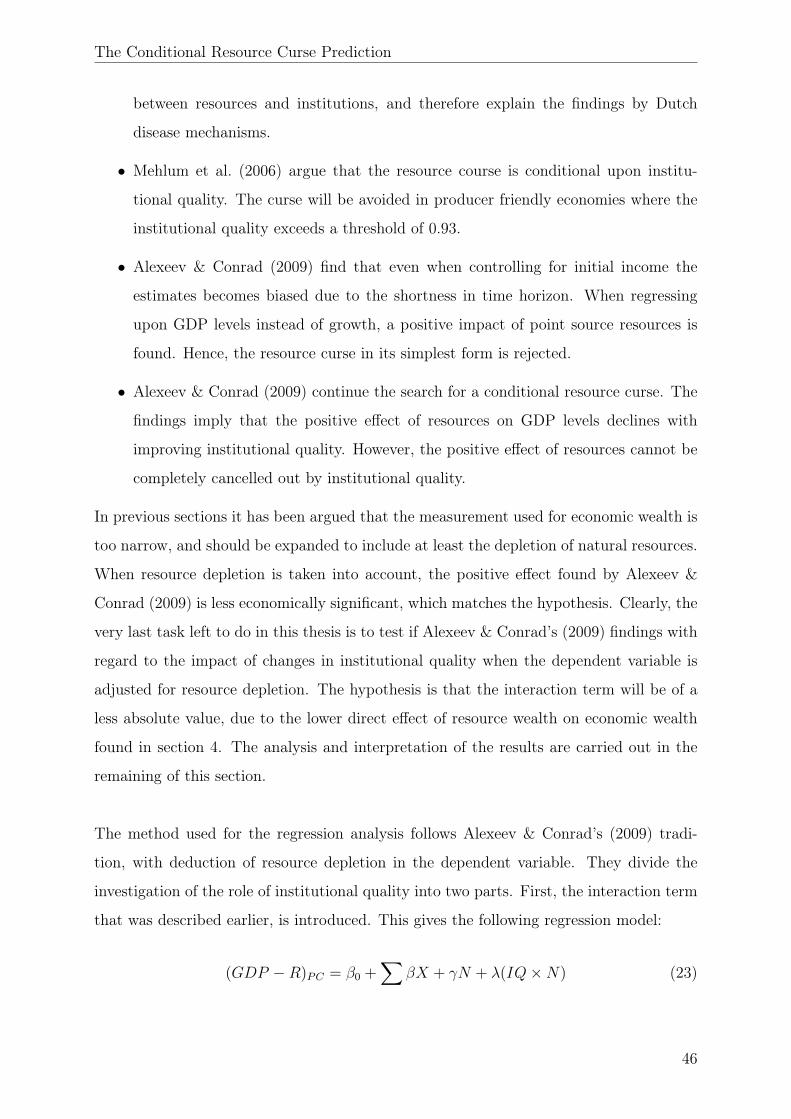
The Conditional Resource Curse Prediction
between resources and institutions, and therefore explain the findings by Dutch
disease mechanisms.
• Mehlum et al. (2006) argue that the resource course is conditional upon institu-
tional quality. The curse will be avoided in producer friendly economies where the
institutional quality exceeds a threshold of 0.93.
• Alexeev & Conrad (2009) find that even when controlling for initial income the
estimates becomes biased due to the shortness in time horizon. When regressing
upon GDP levels instead of growth, a positive impact of point source resources is
found. Hence, the resource curse in its simplest form is rejected.
• Alexeev & Conrad (2009) continue the search for a conditional resource curse. The
findings imply that the positive effect of resources on GDP levels declines with
improving institutional quality. However, the positive effect of resources cannot be
completely cancelled out by institutional quality.
In previous sections it has been argued that the measurement used for economic wealth is
too narrow, and should be expanded to include at least the depletion of natural resources.
When resource depletion is taken into account, the positive effect found by Alexeev &
Conrad (2009) is less economically significant, which matches the hypothesis. Clearly, the
very last task left to do in this thesis is to test if Alexeev & Conrad’s (2009) findings with
regard to the impact of changes in institutional quality when the dependent variable is
adjusted for resource depletion. The hypothesis is that the interaction term will be of a
less absolute value, due to the lower direct effect of resource wealth on economic wealth
found in section 4. The analysis and interpretation of the results are carried out in the
remaining of this section.
The method used for the regression analysis follows Alexeev & Conrad’s (2009) tradi-
tion, with deduction of resource depletion in the dependent variable. They divide the
investigation of the role of institutional quality into two parts. First, the interaction term
that was described earlier, is introduced. This gives the following regression model:
(GDP −R)PC = β0 +∑
βX + γN + λ(IQ×N) (23)
46

The Conditional Resource Curse Prediction
where the estimates will be compared to those found by Alexeev & Conrad (2009) in
equation 22. Due to the potential endogeneity between institutions and GDP, fitted val-
ues of "Rule of law" is created by regressing the explanatory variables absolute latitude,
ethnic fractionalization, the regional dummies and a point source resource measurement.
This produces predicted values for "Rule of law". The process is repeated for all five
measurements of point source resources: Hydrocarbon deposits, the value of oil output,
oil to GDP ratio, mining output and mining to GDP ratio. Using the predicted values
derived by their respective measurement for point source resources, the relationship be-
tween economic and resource wealth can now be found by regressing equation 22 and 23.
The effect of the interaction term will be given by the coefficients θ and λ. The results
are presented in table 8 in the next subsection. The results are tested using ordinary
t-testing, with the results presented in Appendix B. For the adjusted measurement, only
hydrocarbons deposits yields a statistical significant coefficient.
The second part of the investigation looks at the relationship between point source re-
sources and institutional quality directly. A regression is performed in two stages. First,
values are generated to predict the per capita GDP levels the countries could expect to
have if they never where to have had any oil endowment. The predictions are found by
regressing the logarithm of per capita GDP in 1970, alone and adjusted for resource de-
pletion, upon the exogenous geographic variables of absolute latitude, and the dummies
for European population and African and East Asian countries:
GDP1970 = β0 +∑
βX + u (24)
and
(GDP −R)1970 = β0R +∑
βRXi + uR (25)
The footnote R indicates that the coefficient corresponds to resource depletion adjusted
estimation. When the fitted values are obtained, the predicted value for economic wealth
in 1970 is denoted by GDP1970 and (GDP −R)1970. These are used as control variables
when regressing the effect of natural resource endowment on institutional quality, through
47

The Conditional Resource Curse Prediction
the regression models:
IQi = α0,f +∑
αfX + v1,f GDP1970 + v2,fN + ef (26)
and
IQi = α0R,f +∑
αR,fX + v1R,f (GDP −R)1970 + v2R,fN + eR,f (27)
where e is the idiosyncratic error term and the f indicates that the coefficients represent
fitted value effects. These estimates can now be compared to the estimates from regressing:
IQi = α0,o +∑
αoX + v1,oGDP1970 + v2,oN + εo (28)
and
IQi = α0R,o +∑
αR,oX + v1R,o(GDP −R)1970 + v2R,oN + εoR (29)
where the fitted values for GDP and R in equations 26 and 27 are replaced by the observed
values, hence the f’s are replaced by o’s. Here the endogenous negative link between
resources and institutions is eliminated, and the analysis can provide insight of the true
relationship between point source resource wealth and institutional quality.
5.3.1 Results and Interpretation of the Estimates
The first part of the investigation looks at the total effect of the point source resource
wealth on economic wealth when the interaction effect through institutional quality is
included. The results of regressing the models in equations 22 and 23 are presented in
table 8. Robust standard errors are reported in parenthesis. The two last columns provide
the estimates of the interaction terms and the direct effect of the point source resource
respectively.
As described earlier, all the regressions using GDP per capita as dependent variable show
a negative effect of the interaction term. This would imply that countries with weaker
institutions benefit more from natural resources. This does not match the rent seeking
theory. However, the economic significance is small relative to the direct effect of natu-
ral resources. Also, the estimates in regressions 5 and 7 are not statistically significant.
As was discussed earlier, Alexeev & Conrad (2009) interpret the results to mean that
48

The Conditional Resource Curse Prediction
Table 8: Effect of Interaction between Institutions and Natural ResourcesLine Explanatory variable Dependent variable Interaction Term N
1 Hydrocarb. depositsPC GDPPC -0.041 0.056(0.012) (0.014)
2 Hydrocarb. depositsPC (GDP-R)PC -0.029 0.036(0.012) (0.014)
3 Value of oil outputPC GDPPC -0.062 0.095(0.017) (0.017)
4 Value of oil outputPC (GDP-R)PC -0.030 0.046(0.020) (0.024)
5 Oil/GDP ratio GDPPC -0.835 1.139(0.913) (0.679)
6 Oil/GDP ratio (GDP-R)PC 0.387 0.610(0.789) (0.558)
7 Mining/GDP ratio GDPPC -1.534 1.645(2.197) (1.138)
8 Mining/GDP ratio (GDP-R)PC 1.507 1.027(1.879) (1.019)
9 Mining outputPC GDPPC -0.053 0.072(0.913) (0.028)
10 Mining outputPC (GDP-R)PC -0.033 0.033(0.020) (0.029)
Alexeev & Conrad (2009) reports -0.065 as the estimate for the interaction term in line 3. Theregression here is preformed using the exact same data and statistical methods. Regardless, theeconomic significance is only marginal, and the issue is therefore ignored.
countries with good institutions tend to benefit less from the positive effect of natural
resources, relative to countries with poor institutions. The regressions performed with
GDP adjusted for resource depletion as dependent variable basically show the same re-
sults. Here the effect is even less economic significant, and in regression 6 and 8 the effect
becomes positive but, not statistically significant.
The estimates from lines 1 and 2 in table 8 can be used to investigate the effect of a
1 per cent increase in hydrocarbon deposits on economic wealth. The direct effect is a
0.056 per cent increase in GDP per capita and a 0.036 per cent increase in GDP-R per
capita. The total effect will however depend on institutional quality. The mean institu-
tional quality of the sample is 0.0001064. This provides the following effects of a 1 per
49

The Conditional Resource Curse Prediction
cent increase in hydrocarbon deposits in a mean value institutions country:
∂GDPPC = 0.056− 0.041× 0.0001064 = 0.056 (30)
and
∂(GDP −R)PC = 0.036− 0.029× 0.0001064 = 0.036 (31)
As described in section 4, the logistic model specification allows for interpreting the es-
timates as percentage changes. In these examples the total effect is a 0.056 percentage
increase in per capita GDP and 0.036 percentage increase in per capita GDP-R. The effect
of the interaction term is too small to counter the direct positive effect of resource wealth
on economic wealth. But, for the countries scoring the maximum institutional value IQ
= 2.2, the effect of the interaction term counters the direct effect, so that the total effect
is negative:
∂GDPPC = 0.056− 0.041× 2.2 = −0.034 (32)
and
∂(GDP −R)PC = 0.036− 0.029× 2.2 = −0.028 (33)
The neutrality thresholds for GDP and GDP-R respectively, are:
0.056− 0.041(IQ0) = 0 ⇒ IQ0 = 0.056/0.041 = 1.366
0.036− 0.029(IQ0) = 0 ⇒ IQ0 = 0.036/0.029 = 1.241.
The interpretation is that countries with institutional quality scores at 1.366 in total
will have no impact of an marginal increase in hydrocarbon deposits on GDP. For the
impact on resource depletion adjusted GDP to be negligible, the institutional quality only
has to score 1.241. The results clearly do not confirm the traditional hypothesis of a re-
source curse conditional upon institutional quality. Quite on the contrary it seems like
having a high IQ score is a secure pathway towards the resource curse. Notice however
that only 23 out of the 260 countries in the sample scores above the 1.366 threshold, and
only 28 above the 1.241 threshold. This matches Alexeev & Conrad’s (2009) conclusions
50

The Conditional Resource Curse Prediction
that the importance of institutions in the resource curse prediction does not seem to be
of any significance.
The second part of Alexeev & Conrad’s (2009) investigation of the conditional curse
would yield deeper insight to the issue. Running regressions on equations from 24 though
out 29 would produce the fitted values for economic wealth. These could be used to inves-
tigate the change in the impact of resources on institutional quality when using predicted
and observed initial per capita GDP and GDP-R values as control variables. Unfortu-
nately, due to lack of data, these regressions cannot be run for the resource-adjusted
measurement of economic wealth. The results of Alexeev & Conrad (2009) is however
helpful. They indicate that the positive link between natural resources and GDP explains
previous findings of significant negative coefficients for resource endowment in regressions
on institutional quality 3.
When regressing "Rule of Law" on hydrocarbon deposits, the control variable "Observed
per capita GDP in 1970", is estimated to have a positive marginal effect of 0.570. Us-
ing the fitted values for per capita GDP in 1970 estimates a positive marginal effect of
0.508. Both estimates are significant at a 1 per cent level. This indicates that the initial
interaction term overvalues the positive effect of economic wealth on institutional quality.
In addition, the marginal effect of "Hydrocarbon deposits" on "Rule of Law" diminishes
from -0.042 to -0.005 and is no longer statistically significant. When fitted values are
used this trend is visible for all the measurements on point source resources. The effect
of resource wealth on institutional quality declines in absolute value when fitted values
of economic wealth are used as control rather than observed values. On basis of this
Alexeev & Conrad (2009) dismiss the conditional resource curse. Point source resource
endowment does not seem to deteriorate institutional quality, it simply does not improve
it. The findings supports the view that the causality is more likely to go from institutions
to economic growth, and not the other way around, which contradicts the rent-seeking
arguments.
To complete the summation of the discussion in this thesis, the following points are3e.g. in Sala-i-Martin & Subramanian (2003).
51

The Conditional Resource Curse Prediction
added:
• Alexeev & Conrad’s (2009) negative interaction term becomes less negative when
the measurement for economic wealth is expanded to extract depletion of natural
resources. This corresponds with the hypothesis, which was based on the direct pos-
itive effect of resource wealth on economic wealth being less economically significant
when using the resource adjusted GDP rather than GDP alone.
• Alexeev & Conrad (2009) also find that the effect of resource wealth on institutional
quality is insignificant when regressing upon fitted values of initial GDP. This con-
trasts the rent-seeking argument of resource wealth having a negative impact on
institutions, and thereby on economic growth.
The analysis on resource adjusted GDP levels is not able to confirm the existence of a
conditional resource curse. On the contrary, the findings of this section supports Alexeev
& Conrad’s (2009) rejection of the conditional resource curse. Unfortunately, the fitted
values for per capita GDP adjusted for resource depletion could not be obtained, and the
results therefore not confirmed. However, the finding of a smaller absolute value of the
interaction term indicates that institutional quality does not play much of a role in the
relationship between natural resources and economic wealth.
52

Summary and Conclusions
6 Summary and Conclusions
This thesis has aimed to expand the on-going resource curse discussion, adjusting the
measurement of economic wealth for resource depletion. Arguably, by including resource
depletion in addition to GDP in the measurement for economic wealth, the discussion is
more easily approachable to the reality. The reality is complex and the task of economists
is to make simplifications, but not simplifications distorting the truth. By expanding the
measurement, a more correct response of resource extraction on economic wealth can be
found. Resource adjusted GDP still is a simplification, and several more factors could,
and probably should, be included. However, this is a first step of expanding our under-
standing of economic wealth as an indicator of well-being.
Here, the analysis of Alexeev & Conrad (2009) has been used as a benchmark. On
the basis of their analysis, Alexeev & Conrad (2009) rejects the resource curse prediction.
They argue that the negative relationship between economic and natural resource wealth
found in earlier studies is flawed due to the use of GDP growth rates instead of levels.
Using growth rates and controlling for initial income will not prevent the bias of early
resource discovery influencing the initial income level unless a sufficient long time period
is assessed. Sachs & Warner (1995), who was amongst the early debaters advocating the
resource curse, used the growth rate between 1970 and 1989 as dependent variable, and
the income level in 1970 as control. The findings of Alexeev & Conrad (2009) shows that
several countries rich in point source resources started extracting the resource well before
the control year, which might have influenced their initial income level positively. As the
resource income tend to decline towards the end of its quantity, these countries might
therefore appear to have been negatively affected by their resource endowment.
Alexeev & Conrad’s (2009) hypothesis clearly contradicts the resource curse prediction.
However, there exists many theories and hypothesis of why resources could have a nega-
tive impact on economic wealth. The Dutch disease explanation used by Sachs & Warner
(1995) argues that labour is drawn from traded to non-traded sector, where the dynamic
growth effects through learning by doing are smaller. This decreases productivity in the
economy, explaining why natural resource wealth could have a negative impact on eco-
53

Summary and Conclusions
nomic wealth. The structuralist approach, blooming in the 1950’s, blamed the negative
impact on declining terms of trade for the countries specializing in exploitation of natural
resources. Several other researches have blamed the resource curse on internal conflicts,
rent seeking, income inequality and declined saving and investments, amongst other. With
so many arguments of why resource wealth has a negative effect on economic wealth, the
findings of Alexeev & Conrad (2009) is clearly of great importance, questioning the entire
existence of the resource curse prediction in its simplest form.
By deducting resource rents from the GDP levels, the results of Alexeev & Conrad (2009)
have been put to a test. Deducting the income of resource exploitation will make doing
business in natural resources less attractive than when GDP levels are used alone. In this
analysis, the results of Alexeev & Conrad (2009) passed the test. Estimation using the
very same data, in addition to data on resource rents from the same period in time, and
the same methods of estimation, showed that point source resource wealth has a positive
impact on GDP adjusted for resource depletion. With the warnings of the weaknesses of
the analysis in mind, the results support the rejection of the resource curse in its simplest
form. But clearly, the interesting question is not how the average country would respond
to a marginal increase of natural resources, but rather what is the difference between
those countries escaping and those not escaping the resource curse?
The conditional resource curse prediction seeks to find a dimension amongst with resource-
endowed escapers differs from the non-escapers of the curse. Several dimensions are iden-
tified by Torvik (2009). The dimension receiving the most attention from researchers is
institutional quality. Studies using institutional quality as condition for the curse have
found that only those countries with poor institutional quality are affected by the resource
curse (Mehlum et al. 2006). The positive interaction term implies an indirect effect of
resources on economic wealth through institutions. A threshold of institutional quality is
identified to distinguish the curse escapers from the non-escapers. For those nations with
institutional quality falling short of the neutral threshold, there is a negative impact of
natural resources on economic wealth. But, how can it be that "manna from heaven" has
a negative impact on the economy? The threshold divides the so-called producer friendly
economies from the grabber friendly economies. In compliance with rent-seeking theory
54

Summary and Conclusions
it is argued that rent seeking activities is enhanced by natural resource wealth in grab-
ber friendly economies. In sum, resource wealth therefore reduces economic prosperity in
these economies.
Alexeev & Conrad (2009) expands their analysis to test for a resource curse conditional
upon institutional quality. Finding predicted values for income if the resource was never
to be extracted, they are able to put forth highly credible arguments of the significance
of resource wealth on institutional quality. An analysis is conducted with an interaction
term, which is found to have a negative effect while the direct effect is still positive. The
economic significance of the interaction term is however small, and it is therefore con-
cluded that the positive effect of natural resources on economic wealth is simply more
prominent in poorly institutionalized countries. This statement is put to a test by includ-
ing resource depletion to the measurement for economic wealth. In doing so, it is found
that the absolute value of the negative interaction term is reduced. Also the direct posi-
tive effect of point source resources is reduced. It makes sense that all effects of resources
on economic wealth is reduced when the clearly positive effect of resource rent is deducted
from the equation. The results of testing the conditional curse on resource adjusted GDP
are however questionable, as both the economical and statistical significance is weak.
More work should be conducted to further capture the reality when searching for the
relationship between natural resource wealth, economic wealth and other factors affecting
the relationship. Hopefully, future studies will continue to expand the analysis, so that
economic theory can provide the decision makers with as accurate information as possible
on how a country can exploit its natural resources efficiently.
55
REFERENCES
References
Acemoglu, D., Johnson, S. & Robinson, J. A. (2001), ‘The Colonial Origins of Com-
parative Development: An Emperical Investigation’, American Economic Review
91(5), 1369–1401.
Acemoglu, D. & Robinson, J. (2012), Why Nations Fail: The Origins of Power, Prosper-
ity, and Poverty, Crown Business.
Alexeev, M. & Conrad, R. (2009), ‘The Elusive Curse of Oil’, The Review of Economics
and Statistics 91(3), 586–598.
Andersen, J. J. & Aslaksen, S. (2013), ‘Oil and Political Survival’, Journal of Development
Economics 100(1), 89–106.
Baum, C. F., Schaffer, M. E. & Stillman, S. (2003), ‘Instrumental variables and GMM:
Estimation and testing’, The Stata Journal 3(1), 1–31.
Cust, J. & Harding, T. (2014), ‘Institutions and the Location of Oil Exploration’, Oxford
Centre for the Analysis of Resource Rich Economies.
Cypher, J. M. & Dietz, J. L. (2009), The Process of Economic Development, 3 edn,
Routledge, 2 Park Square, Milton Park, Abingdon, Oxon OX14 4RN.
Dabla-Norris, E. & Wade, P. (2001), ‘Rent Seeking and Endogenous Income Inequality’,
IMF Working Paper .
Everett, G. & Wilks, A. (1999), The World Bank’s Genuine Savings Indicator: a Useful
Measure of Sustainability?, The Bretton Woods Project.
Hueting, R. (1987), ‘Economic Aspects of Environmental Accounting’, Journal of Inter-
disciplinary Economics 2(1), 55–71.
Kaufmann, D., Kraay, A. & Mastruzzi, M. (2005), ‘Governance Matters IV: Governance
Indicators for 1996-2004’, World Bank Policy Research Working Paper 3630.
Leighton, T. R. (2004), Using Statistics in Econometrics, McGraw-Hill Education, Shop-
penhangers Road, Maidenhead Berkshire, SL6 2QL.
56

REFERENCES
Mehlum, H., Moene, K. & Torvik, R. (2006), ‘Institutions and the Resource Curse’, The
Economic Journal 116(508), 1–20.
The World Bank (2006), Where is the Wealth of Nations? Measuring Capital for the 21st
Century, The International Bank for Reconstruction and Development/The World
Bank, 1818 H Street, NW Washington, DC 20433.
The World Bank (2011), The Changing Wealth of Nations: Measuring Sustainable De-
velopment in the New Millennium, The International Bank for Reconstruction and
Development / The World Bank, 1818 H Street NW Washington DC 20433.
The World Commission on Environment & Development (1987), ‘Report of the World
Commission on Environment and Development: Our Common Future’.
North, D. C. (1991), ‘Institutions’, Journal of Economic Perspectives 5(1), 97–112.
Oman, C. P. & Wignaraja, G. (1991), Postwar Evolution of Development Thinking, The
Macmillan Press LTD, Houndmills, Basingstoke, Hampshire RG21 2XS.
Pearce, D. W. & Atkinson, G. D. (1993), ‘Capital Theory and the Measurement of Sus-
tainable Development: An indicator of "weak" sustainability’, Ecological Economics
8(2), 103–108.
Perman, R., Ma, Y., Common, M., Maddison, D. & McGilvray, J. (2011), Natural Re-
source and Environmental Economics, 4 edn, Pearson Education Limited, Edinburgh
Gate, Harlow, Essex CM20 2JE, England.
Sachs, J. D. & Warner, A. M. (1995), ‘Natural Resource Abundance and Economic
Growth’, NBER Working Paper No. 5398.
Sachs, J. D. & Warner, A. M. (1997), ‘Sources of Slow Growth in African Economies’,
Journal of African Economics 6, 335–376.
Sala-i-Martin, X., Doppelhofer, G. & Miller, R. I. (2004), ‘Determinants of Long-Term
Growth: A Bayesian Averaging of Classical Estimates (BACE) Approach’, American
Economic Review 94(4), 813–835.
Sala-i-Martin, X. & Subramanian, A. (2003), ‘Adressing a Natural Resource Curse: An
Illustration from Nigeria’, NBER Working Paper no. 9804.
57

REFERENCES
Torvik, R. (2009), ‘Why do some resource-aboundant countries succeed while others do
not?’, Oxford Review of Economic Policy 25(2), 241–256.
van der Ploeg, F. (2011), ‘Natural Resources: Curse or Blessing?’, Journal of Economic
Literature 49(2), 366–420.
Verbeek, M. (2013), A Guide to Modern Econometrics, 4 edn, John Wiley & Sons, Ltd.,
The Atrium, Southern Gate, Chichester, West Sussex, PO19 8SQ, United Kingdom.
Woolridge, J. M. (2013), Introductory Econometrics: A Modern Approach, 5 edn, South-
Western, Cengage Learning, 5191 Natorp Boulevard, Mason OH 45040, USA.
58

The Gauss-Markov Theorem
A The Gauss-Markov Theorem
Section 3.3 briefly describes the Gauss-Markov assumptions, and states the Gauss-Markov
theorem that under these assumptions the OLS estimators are BLUE. Here, the proof will
be derived.
The assumptions, following Woolridge (2013), states that:
• Assumption 1: The Population Model is Linear in its Parameters
The population model can then be written
y = β0 + β1x1 + ...+ βkxk + u (34)
where β0, β1, ..., βk are unknown coefficients, x1, ..., xk are the explanatory indepen-
dent variables, and u is the unobserved random error.
• Assumption 2: Random Sampling
All the n observations of x1,i, ..., xk,i, yi (where i = 1, 2, .., n) in the sample is random.
• Assumption 3: No Perfect Collinearity
None of the explanatory variables are constant, and there is no exact linear rela-
tionships among the explanatory variables in the sample.
• Assumption 4: Zero Conditional Mean
Given any value of the explanatory variables, the idiosyncratic error term u is ex-
pected to take the value zero:
E(u|x1, ..., xk) = 0 (35)
• Assumption 5: Homoskedasticity
Given any value of the explanatory variables, the idiosyncratic error term u has the
same variance:
V ar(u|x1, ..., xk) = σ2 (36)
Lets first derive the OLS estimator and find the proof that the OLS estimator is unbiased.
This will be done in matrix form, expressed by bold letters. The population model is then
59

The Gauss-Markov Theorem
assumed to take the form:
y = Xβ + u (37)
where y is a n×1 vector of observations of the dependent variable, X is a matrix of the
n×(k+1) observed explanatory variables and the constant term, β is a (k+1) vector of
coefficients and u is a (N+1) vector of unobservable error. Estimates of β and u must
be found, and these will be denoted by β and u. The OLS estimates are obtained by
minimizing the sum of squared residuals, SSR. Formally:
Min SSR = u´u = (u1, u2, ..., uN)
u1
u2...
uN
= u12 + u2
2 + ...+ uN2 =
N∑i=1
ui2 (38)
The model can be rewritten to yield:
u = y −Xβ (39)
which yields the squared sum of residuals:
SSR = (y−Xβ)´(y−Xβ) = (y´−β´X‘)(y−Xβ) = y´y−y´Xβ−β´X´Xβ (40)
By finding the derivate of SSR with respect to β the β‘s minimizing SSR is found, and
these will be the OLS-estimates:
∂SSR
∂β= 0−X´y −X´y + 2X´Xβ = 0 (41)
The OLS-estimators is solved using simple matrix rules:
ˆβOLS = (X´X)−1X´y (42)
60

The Gauss-Markov Theorem
The estimator is unbiased if its expectation equals β. Inserting for y = Xβ + u in the
expression above, yields:
ˆβOLS = (X´X)−1X´Xβ + (X´X)−1X´u = β + (X´X)−1X´u (43)
Taking the expectation yields:
E( ˆβOLS) = β + (X´X)−1X´E(u) (44)
Using Assumption 4 of zero conditional mean, the last term vanishes, so that:
E( ˆβOLS) = β (45)
This proves that ˆβOLS is an unbiased estimate of β.
To prove that the OLS estimator is the best linear unbiased estimator, given the Gauss-
Markov assumptions, it must be proven that the variance of the OLS estimator always will
be smaller or equal to the variance of any other linear unbiased estimator. Lets denote
the OLS estimator as βOLS and the other unbiased estimator as β. It must then be true
that:
V ar(βOLS) ≤ V ar(β) (46)
The variance of the OLS-estimator is derived by exploiting the matrix rule that the
variance of an expression AX equals Avar(X)A´. Using the rules that (AB)´ =
B´A´ and (A−1)´ = (A´)−1, it is now true that:
var(βOLS) = (X´X)−1X´var(y)X(X´X)−1 (47)
Assumptions 3 and 5 implies that var(U |X) = var(y) = σ2I, where I is the identity
matrix. The variance of βOLS can now be expressed as:
var( ˆβOLS) = (X´X)−1σ2IX(X´X)−1 = σ2(X´X)−1 (48)
61

The Gauss-Markov Theorem
To prove that this variance is at least as small as the variance of an alternative linear
estimator, the alternative estimator is now defined as:
(β) = ˆβOLS +Dy = (X´X)−1X´y +Dy = [(X´X)−1X´ +D]y (49)
Notice that the estimator β only is unbiased whenDX = 0. Using the same matrix rules
as above, it is found that:
var(β) = σ2[(X´X)−1 +DD´] = var( ˆβOLS) + σ2DD´ (50)
Since a matrix multiplied with its inverse always will be a positive semi defined matrix,
the last term will always be larger or equal to zero. This finishes the proof that there
exists no other linear unbiased estimator with a variance smaller than the OLS-estimator.
Given the Gauss-Markov assumptions, the Gauss-Markov theorem holds.
62

Test Results
B Test Results
Tables 9 to 15 reports the results of the test procedures described in section 3.
t-statistics
All t-test are preformed under the null hypothesis: H0 : βm = 0 where βm is the coefficient
of the natural resource. The null hypothesis is tested against the two-sided alternative
HA : βm 6= 0. This means that the null hypothesis is rejected whenever the t-value exceeds
the critical value for the following levels of significance:
• 1% level: t0.01 = 2.62, indicated by ***
• 5% level: t0.05 = 1.98, indicated by **
• 10% level: t0.10 = 1.66, indicated by *
F-statistics
The F-values of the instrumented estimations are also reported below. They all satisfy
the rule-of-thumb as they all exceed a value of 10.
The Hausman Test
The Hausman test results are obtained through STATA, like described in section 3. All
tests are run under the H0 : The instrument is exogenous. Under this hypothesis the test
statistic is chi-squared distributed with 1 degree of freedom, as only the one instrument
"Rule of Law" is tested for endogeneity. H0 is rejected whenever the test statistic exceeds
the critical value for the following levels of significance:
• 1% level: t0.01 = 6.63, indicated by *
• 5% level: t0.05 = 3.84, indicated by **
• 10% level: t0.10 = 2.71, indicated by ***
63

Test Results
Sargan Test
The Sargan test statistics is here found though regression in STATA. The procedure is
described in section 3. The test statistic reported in table 10 and 13 has 2 degrees of free-
dom since there are 3 instruments and 1 endogenous regressor. The Sargan test statistic
in table 11 and 14 has only 1 degree of freedom as these are estimated with only 2 in-
struments. All the absolute values of the Sargan test statistics are found to be well below
the critical value of rejection for a 1% level of significance, which are 2.71 and 4.61 with
1 and 2 degrees of freedom respectively. The null hypothesis that the model is correctly
overidentified is therefore not rejected in neither of the estimations.
Tables 9 to 12 reports the test statistics for the regressions in section 4. Table 13 re-
ports t-test statistics for the estimates on the conditional curse in section 6.
Table 9: Test statistics of estimates from table 2Explanatory variable Dependent variable t-value
Hydrocarb. depositsPC GDPPC 3.79***Hydrocarb. depositsPC (GDP-R)PC 2.67***Value of oil outputPC GDPPC 4.17***Value of oil outputPC (GDP-R)PC 2.30**Oil/GDP ratio GDPPC 2.17**Oil/GDP ratio (GDP-R)PC 1.11
Table 10: Test statistics of estimates from table 3Explanatory var. Dependent var. t-value F-value Hausman Sargan
Hydrocarb. dep.PC GDPPC 5.11*** 10.931 6.29* 2.21Hydrocarb. dep.PC (GDP-R)PC 2.42** 10.772 6.94 3.10Value of oil outputPC GDPPC 5.77*** 12.496 2.99** 3.12Value of oil outputPC (GDP-R)PC 2.28** 12.910 3.52** 3.00Oil/GDP ratio GDPPC 4.01*** 12.041 5.26* 0.460Oil/GDP ratio (GDP-R)PC -0.01 12.448 5.46* 1.28
64

Test Results
Table 11: Test statistics of estimates from table 4Explanatory var. Dependent var. t-value F-value Hausman Sargan
Hydrocarb. dep.PC GDPPC 5.03*** 21.287 2.78** 0.00Hydrocarb. dep.PC (GDP-R)PC 3.10*** 21.130 6.81 0.01Value of oil outputPC GDPPC 7.45*** 21.856 6.11* 0.00Value of oil outputPC (GDP-R)PC 4.10*** 22.030 9.04 0.04Oil/GDP ratio GDPPC 3.60*** 21.240 9.46 0.02Oil/GDP ratio (GDP-R)PC 1.73* 21.290 10.79 0.04
Table 12: Test statistics of estimates from table 5Explanatory variable Dependent variable t-value
Mining outputPC GDPPC 3.40***Mining outputPC (GDP-R)PC 2.21**Mining/GDP ratio GDPPC 2.34**Mining/GDP ratio (GDP-R)PC 1.56
Table 13: Test statistics of estimates from table 6Explanatory var. Dependent var. t-value F-value Hausman Sargan
Mining outputPC GDPPC 3.13*** 10.629 3.50** 1.84Mining outputPC (GDP-R)PC 1.35 11.407 3.80** 2.09Mining/GDP ratio GDPPC 1.71* 11.006 5.64* 0.63Mining/GDP ratio (GDP-R)PC -0.68 11.554 5.61* 1.13
Table 14: Test statistics of estimates from table 7Explanatory var. Dependent var. t-value F-value Hausman Sargan
Mining outputPC GDPPC 2.81*** 20.724 7.92 0.44Mining outputPC (GDP-R)PC 1.33 20.743 11.02 0.03Mining/GDP ratio GDPPC 3.29*** 20.159 9.22 0.81Mining/GDP ratio (GDP-R)PC 1.22 21.125 11.07 0.05
65

Test Results
Table 15: Test statistics of estimates from table 8Line Explanatory var. Dependent var. t-value of interaction term t-value of N
1 Hydrocarb. dep.PC GDPPC -3.39*** 3.93***2 Hydrocarb. dep.PC (GDP-R)PC -2.35** 2.25**3 Value of oil outputPC GDPPC -3.64*** 4.47***4 Value of oil outputPC (GDP-R)PC -1.49 1.93*5 Oil/GDP ratio GDPPC -0.91 1.68*6 Oil/GDP ratio (GDP-R)PC 0.49 1.097 Mining/GDP ratio GDPPC -0.70 1.458 Mining/GDP ratio (GDP-R)PC 0.80 1.019 Mining outputPC GDPPC -2.76*** 2.54**10 Mining outputPC (GDP-R)PC -1.66 1.15
66

Full Presentation of the Regression Results
C Full Presentation of the Regression Results
All regression results are presented here. The data material is available on request.
Table 16: OLS estimation results on oil wealthRegressors Dependent variable
GDP GDP-R GDP GDP-R GDP GDP-RAbsolute latitude 0.037 0.040 0.038 0.040 0.038 0.041European pop. 1.340 1.386 1.300 1.359 1.433 1.418Latin Am. country 1.018 1.070 0.926 1.001 1.056 1.067East Asian country 1.703 1.714 1.668 1.704 1.767 1.759Hydrocarb.deposit 0.059 0.041Value of oil output 0.096 0.054Oil/GDP ratio 1.507 0.793Constant 6.711 -0.366 6.593 -0.412 6.631 -0.387
Table 17: OLS estimation results on oil wealth with the interaction termRegressors Dependent variable
GDP GDP-R GDP GDP-R GDP GDP-RRule of Law×N -0.041 -0.029 -0.062 0.030 -0.835 0.387Rule of Law 1.142 1.181 1.119 1.126 1.146 1.097Ethnic fractionalization -0.179 -0.277 -0.474 -0.522 -0.453 -0.506European pop. 0.019 -0.002 0.121 0.838 -0.028 0.061East Asian country 0.530 0.569 0.534 0.576 0.557 0.615Latin Am. country 0.763 0.781 0.607 0.679 0.750 0.746Hydrocarb.deposit 0.056 0.036Value of oil output 0.095 0.046Oil/GDP ratio 1.139 0.610Constant 7.937 0.971 7.912 0.997 7.988 1.027
67

Full Presentation of the Regression Results
Table 18: OLS estimation results on mineral wealthRegressors Dependent variable
GDP GDP-R GDP GDP-RAbsolute latitude 0.036 0.039 0.038 0.040European pop. 1.377 1.489 1.300 1.467Latin Am. country 0.941 1.046 0.926 1.070East Asian country 1.628 1.734 1.668 1.734Mining/GDP ratio 2.603 1.618Mining output 0.094 0.061Constant 6.463 -0.509 6.567 -0.438
Table 19: OLS estimation results on mineral wealth with the interaction termRegressors Dependent variable
GDP GDP-R GDP GDP-RRule of Law×N -1.533 1.507 -0.053 -0.033Rule of Law 1.130 0.992 1.192 1.197Ethnic fractionalization -0.486 -0.434 -0.474 -0.511European pop. 0.051 0.271 0.129 0.077East Asian country 0.744 0.835 0.552 0.573Latin Am. country 0.702 0.716 0.638 0.698Mining/GDP ratio 1.645 1.027Mining output 0.072 0.033Constant 7.914 0.929 7.836 0.965
68
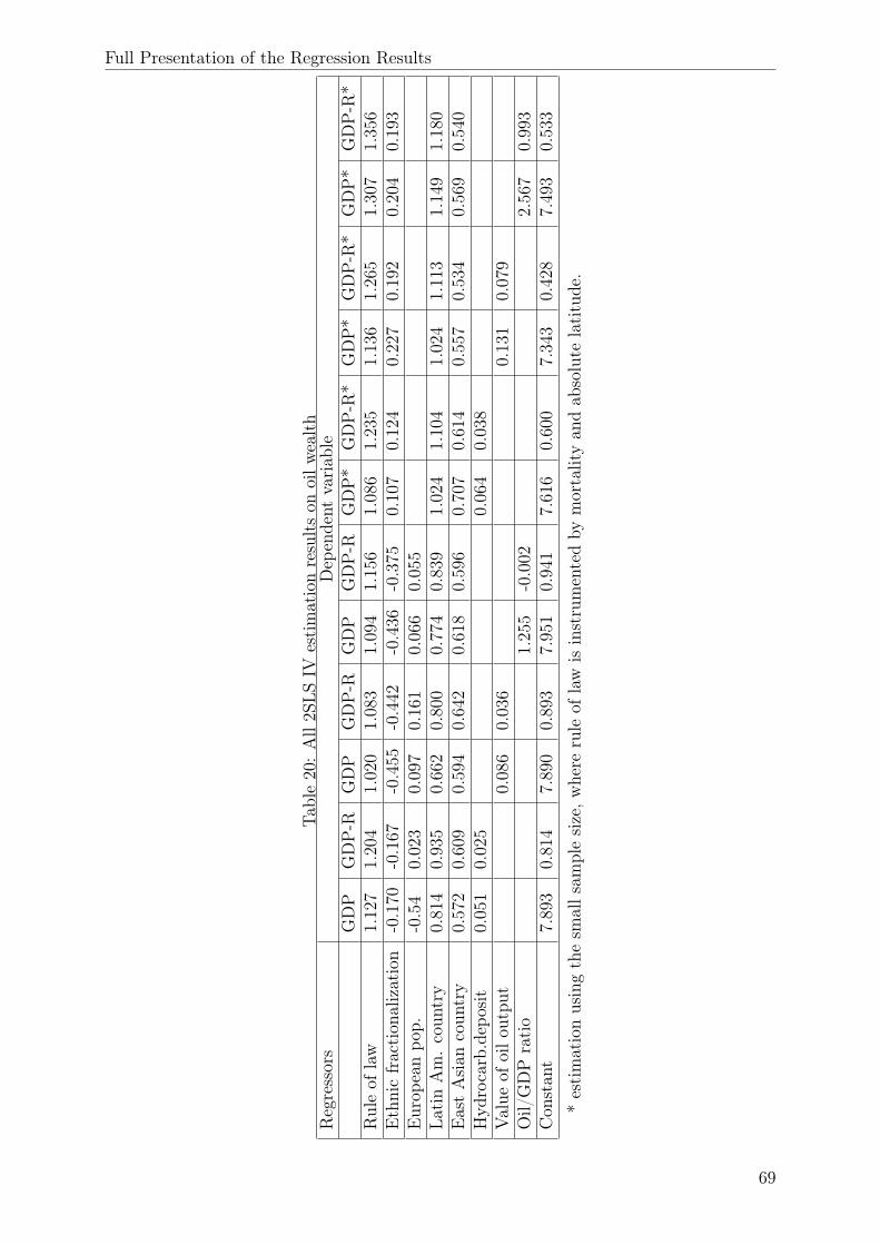
Full Presentation of the Regression Results
Table20
:All2S
LSIV
estimationresultson
oilw
ealth
Regressors
Dep
endent
variab
leGDP
GDP-R
GDP
GDP-R
GDP
GDP-R
GDP*
GDP-R
*GDP*
GDP-R
*GDP*
GDP-R
*Ruleof
law
1.12
71.20
41.02
01.08
31.09
41.15
61.08
61.23
51.13
61.26
51.30
71.35
6Ethnicfraction
alization
-0.170
-0.167
-0.455
-0.442
-0.436
-0.375
0.10
70.12
40.22
70.19
20.20
40.19
3Europ
eanpo
p.-0.54
0.02
30.09
70.16
10.06
60.05
5La
tinAm.coun
try
0.81
40.93
50.66
20.80
00.77
40.83
91.02
41.10
41.02
41.11
31.14
91.18
0EastAsian
coun
try
0.57
20.60
90.59
40.64
20.61
80.59
60.70
70.61
40.55
70.53
40.56
90.54
0Hyd
rocarb.dep
osit
0.05
10.02
50.06
40.03
8Value
ofoilo
utpu
t0.08
60.03
60.13
10.07
9Oil/
GDP
ratio
1.25
5-0.002
2.56
70.99
3Con
stan
t7.89
30.81
47.89
00.89
37.95
10.94
17.61
60.60
07.34
30.42
87.49
30.53
3
*estimationusingthesm
alls
amplesize,w
here
rule
oflaw
isinstrumentedby
mortalityan
dab
solute
latitude.
69

Full Presentation of the Regression Results
Table21
:All2S
LSIV
estimationresultson
mineral
wealth
Regressors
Dep
endent
variab
leGDP
GDP-R
GDP
GDP-R
GDP*
GDP-R
*GDP*
GDP-R
*Ruleof
law
1.04
21.09
71.12
01.17
91.19
01.30
81.30
01.35
3Ethnicfraction
alization
-0.432
-0.422
-0.416
-0.339
0.28
80.23
50.21
60.20
6Europ
eanpo
p.0.08
10.15
00.02
2-0.005
LatinAm.coun
try
0.69
00.81
70.74
80.83
81.05
61.14
11.09
71.16
1EastAsian
coun
try
0.57
40.64
60.56
10.56
30.62
50.56
30.46
70.50
0Miningou
tput
0.06
20.02
50.08
20.03
6Mining/
GDP
ratio
1.44
4-0.488
4.50
61.62
1Con
stan
t7.81
70.85
97.94
90.96
37.29
30.43
97.40
80.50
3
*estimationusingthesm
alls
amplesize,w
here
rule
oflaw
isinstrumentedby
mortalityan
dab
solute
latitude.
70