Natural disasters and labor markets

Martina Kirchbergera∗

a Centre for the Study of African Economies,

Department of Economics, University of Oxford

Abstract:While it is clear that natural disasters have serious welfare consequences for affected pop-ulations, less is known with respect to how local labor markets in low income countriesadjust to such large shocks, in particular the general equilibrium effects of the increasein the demand for construction as well as the inflow of resources in the aftermath ofnatural disasters. Building on the literature on local labor markets (Moretti, 2010a,b),this paper investigates whether there is evidence that changes in the relative prices ofnon-tradable to tradable goods induced by a demand shock due to a natural disaster leadto a reallocation of employment and wage premia across sectors. Combining data fromthe Indonesia Family Life Survey and the US Geological Survey we study the effect ofearthquakes on local labor markets in Indonesia. We find evidence for sectoral reallo-cation of workers as well as significant and persistent wage premia. Employment in theconstruction sector increases significantly and contracts in the agriculture sector in thetwo years after an earthquake takes place in a community. There appear to be substan-tial labor market rigidities since even after sectoral mobility has taken place, individualsemployed in sectors producing non-tradable goods experience significantly higher wagegrowth in communities that were struck by an earthquake. These effects are homogenousalong the quantiles of the conditional income growth distribution. Thereby, they neutral-ize otherwise occurring differential earnings growth patterns across sectors and operateas pure location shifts of the income distribution rather than altering the shape.

Keywords: local labor markets, natural disasters, Dutch diseaseJEL classification: J20, Q54, O10

∗Correspondence: Centre for the Study of African Economies (CSAE), Department of Economics,Manor Road Building, Oxford OX1 3UQ, UK; Email: martina.kirchberger@economics.ox.ac.uk

1

1 Introduction

Despite the total number of natural disasters being roughly equal for high and low

income countries, their impact in terms of fatalities has been found to be substantially

higher in low income countries (Stromberg, 2007). About 99% of people affected

by natural disasters over the period of 1970-2008 reside in the Asia-Pacific region,

Latin America and the Caribbean or Africa, accounting only for 75% of the world

population (Cavallo and Noy, 2009). It is clear that there are vast welfare and asset

losses associated with natural disasters which often, and luckily so, are followed by

large inflows of resources for emergency relief and reconstruction. In many cases, the

housing sector accounts for a significant proportion of total damage and losses: for

example, 40% of the damage and losses from the 2010 earthquake in Haiti is due to

destroyed and damaged housing (Government of Haiti et al, 2010). This figure is even

higher for the 2009 West Sumatra earthquake (BNPB et al, 2009) and about half for

the 2006 earthquake in Yogyakarta and Central Java (BAPPENAS, 2006). Once the

emergency phase is over, aid flows often last for several years following the disaster.

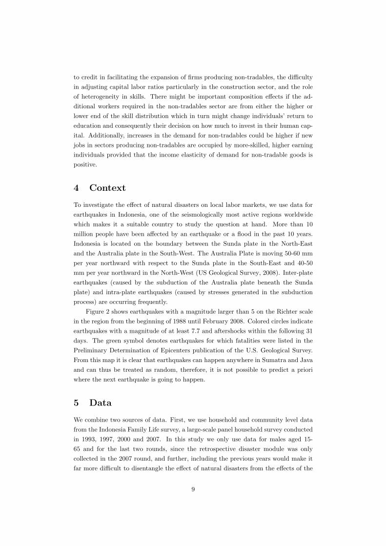
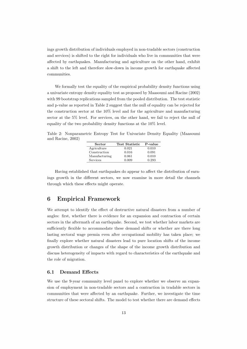
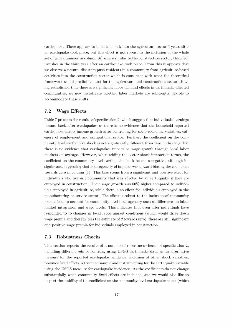
Figure 1: Post Tsunami Fund Allocations by Sector, Aceh, Indonesia

Source: World Bank (2008).

Figure 1 shows that post-tsunami allocations to the housing sector in Aceh in

Indonesia amount to $US 1.6 billion, which is equivalent to 25% of total reconstruction

funding and 30% of Aceh’s regional GDP. As the panel on the right shows, resource

flows can last over several years.

However, we know little with respect to how local labor markets in low and

middle income countries adjust to large destructive shocks such as earthquakes and

hurricanes, in particular how flexible labor markets are to accommodate such large

demand shocks due to the increase in the demand for construction as well as the

inflow of resources in the aftermath of natural disasters.

A substantial body of literature in development economics explores how shocks

impact on households along a number of dimensions, including households’ ability

2

to smooth consumption, ex-ante and ex-post coping strategies as well as short and

long-term effects of shocks on a range of outcomes such as consumption, schooling,

health and child work (Townsend, 1994; Paxson, 1992; Udry, 1995; Dercon, 2004).

Employment in the non-agricultural sector has been found to be an important strategy

for agricultural households to diversify their portfolio ex-ante as well as ex-post (Rose,

2001; Kochar, 1999; Takasaki, Barham, and Coomes, 2010; Cameron and Worswick,

2003). A few studies investigate the impact of weather shocks (droughts, floods) on

labor markets, and they focus either entirely on the agricultural labor market or only

distinguish between agricultural vs non-agricultural workers, rural vs urban wages

or livelihood strategies but not between employment sectors (Jayachandran, 2006;

Mueller and Osgood, 2009; Mueller and Quisumbing, 2010; Banerjee, 2007; Van den

Berg, 2010).

This paper investigates whether there is evidence for general equilibrium effects

through changes in the relative price of non-tradable to tradable goods, such as a

reallocation of employment and wage premia between sectors producing tradable vs

non-tradable goods. We find evidence of sectoral reallocation of workers as well as

significant and long lasting wage premia for individuals employed in sectors produc-

ing non-tradables. The proportion of individuals employed in agriculture increases by

2.7% and 5.9% points in the first and second year, respectively, following an earth-

quake. This is accompanied by a contraction in the agriculture sector, where employ-

ment is reduced by 4.1% points one year after the earthquake and by 9.1% points two

years after the earthquake took place. There appear to be substantial labor market

rigidities since even after sectoral mobility has taken place, individuals employed in

sectors producing non-tradable goods enjoy significantly higher wage growth. Indi-

viduals employed in the construction and service sector in a community that was hit

by an earthquake experienced about 60-100% and about 30-40%, respectively, higher

earnings growth between 2000 and 2007 compared to individuals employed in agri-

culture. These effects are fairly homogenous along the quantiles of the conditional

income growth distribution. Thereby, they neutralize otherwise arising differential

earnings growth patterns across sectors and operate as pure location shifts of the

income distribution rather than altering the shape.

The paper is structured as follows. Section 2 presents some evidence from related

studies; section 3 provides a conceptual framework to outline the channels through

which natural disasters might impact on local labor markets; sections 4 and 5 describe

the Indonesian context and the data. The econometric framework is presented in

section 6 and section 7 discusses the results. Section 8 concludes.

2 Literature

The existing evidence on how natural disasters work through economies, in particular

labor markets, is scarce. We start by presenting some findings from the macro liter-

3

ature on the effects of natural disasters on GDP and GDP growth; we then review

evidence from the micro literature on the impact of natural disasters on outcomes

such as poverty and migration where we focus on destructive natural disasters. As

there is little evidence on the effect of destructive natural disasters on labor markets,

in addition to destructive natural disasters, we also include studies that investigate

the impact of weather shocks on wages and labor markets in low and middle income

countries. Finally, we discuss insights from the labor economics literature on the im-

pact of demand side shocks on sectoral labor market dynamics and the existence of

local multipliers.

There is an ongoing debate in macroeconomics on whether natural disasters harm

economic growth, foster it, have impacts only under certain conditions, or no impact

at all. For example, Hochrainer (2009) finds that natural disasters have significant

negative effects on GDP in the medium run; higher aid rates and higher remittances

lessen the adverse effects and higher capital stock losses worsen the negative effects.

Noy (2009) finds stronger negative effects of natural disasters for developing countries

and smaller economies compared to developed or bigger economies. On the other

hand, Skidmore and Toya (2002) find a positive correlation between the frequency

of climatic disasters and growth in total factor productivity and GDP. Cuaresma,

Hlouskova, and Obersteiner (2008) argue that ’creative destruction’ and technology

upgrading in the aftermath of disasters can take place, but only at high levels of

economic development. Finally, Loayza, Olaberrıa, Rigolini, and Christiaensen (2009)

find that the effect of natural disasters is heterogenous with regard to the type and

severity of a natural disaster and the level of development of a country; further, they

find evidence for significant differences in impacts by sector. Examining the effect

of hurricanes in the US on local growth rates, Strobl (2010) finds that hurricanes

significantly reduce county-level growth rates but the effect is fairly short-lived and

disappears one year after the earthquake.

Several studies look at the impact of natural disasters on poverty, and a few stud-

ies on migration. Baez and Santos (2008) investigate the impact of two earthquakes

in El Salvador that struck in early 2001. They use the last two rounds of the BASIS

El Salvador Rural Household Survey and find that household income per capita is

reduced by one third for households in the upper half of the shaking distribution;

although not statistically significant, severity and depth of poverty increases. Pre-

mand (2008) estimates micro growth models using data from the Nicaraguan LSMS,

focusing on agricultural households, and finds moderate short term effects of hurri-

cane Mitch on consumption growth but no evidence for persistence. Halliday (2006)

investigates the impact of harvest and livestock loss as well as two earthquakes on

the probability of sending a migrant to the United States as a coping strategy in the

aftermath of a disaster. He finds that earthquakes reduce the likelihood of sending

a migrant to the U.S. across all wealth levels. From this he concludes that it is not

due to liquidity constraints that households don’t send a migrant in response to an

4

earthquake shock but rather through the need for the migrant at home. While he

observes an increase in remittances following harvest and livestock loss, remittances

tend to be lower after earthquakes. Yang (2008) on the other hand, using the same

data for El Salvador, argues that the decrease in migration following an earthquake

is due to liquidity constraints. Datt and Hoogeveen (2003) use data from the Philip-

pines to evaluate the impact of a (i) labor market shock alone due to the Asian Crisis;

(ii) El Nino shock (drought) alone and (iii) joint labor market and El Nino shock

on consumption and income. They find that largest share of the overall impact on

poverty is attributed to the El Nino shock as opposed to the labor market shock.

A few studies investigate the link between extreme weather events such as floods,

droughts or hurricanes on wages and employment. Jayachandran (2006) indirectly

examines the relationship between wages and weather shocks in the agricultural labor

market, instrumenting yields with rainfall shocks in a regression of agricultural wages

on yields, variables influencing the elasticity of labor supply and other covariates.

Using data from a panel of 257 districts in India, she finds that agricultural wages

respond more to productivity shocks in the absence of financial institutions and mi-

gration opportunities, factors that would make labor supply more elastic. Estimating

a similar reduced form model for Brazil, Mueller and Osgood (2009) find negative

wage effects of droughts on rural wages that last up to five years.

Mueller and Quisumbing (2010) use data from the Bangladesh Flood impact panel

household survey to evaluate the impact of the 1998 flood. They find short time wage

losses for agricultural workers and long-term wage losses for nonagricultural workers;

short term drops in wages are sharper for communities that are located further away

from markets but distance to a market is then positively correlated with wages in

the long term. Banerjee (2007) also looks at the impact of floods in Bangladesh on

wages of male agriculture workers and finds negative effects if floods occur in the dry

harvest season but positive effects if the floods occur during the growing period of

wet-season crops.

Belasen and Polachek (2008, 2009) investigate the labor market consequences of

hurricanes in Florida, exploiting differences in county-level earnings and employment

rates calculated from quarterly data. Employing a Generalized Difference in Differ-

ence technique, they find a positive earnings effect and a negative employment effect

for counties struck by a hurricane while neighboring counties experience a negative

earnings effect but no employment effect. Analyzing sectoral composition, they find

that earnings and employment effects move together for both directly affected and

neighboring counties, with positive effects on wages and employment in the construc-

tion and service sector for directly affected counties1.

A related literature focuses on general equilibrium effects of demand shocks in

local labor markets with evidence mainly from developed countries. Moretti (2010b)

1Some studies use hurricanes as natural experiments to investigate the impact of migration onreceiving labor markets, for example see McIntosh (2008); Silva, McComb, Moh, Schiller, and Vargas(2010).

5

uses data from the US Census of Population and finds a significant relationship be-

tween changes in the number of jobs in a city in the tradable sector and the non-

tradable sector. Each additional job in the tradable sector is associated with 1.6 jobs

created in the non-tradable sector in a city or 2.5 additional jobs in the non-tradable

sector if the additional job in the tradable sector is taken up by a worker with some

college education or more. Carrington (1996) finds a significant short run employment

multiplier from the construction of the Trans-Alaskan Pipeline System in other parts

of the economy. Kline (2008) uses data for the US oil and gas field services industry

and investigates labor market responses to changes in the price of crude petroleum.

He finds that the labor market quickly reallocates across sectors in response to price

changes, but substantial wage premia are necessary to induce the reallocation. Wage

premia emerge quite slowly and peak only as labor adjustment ends and then slowly

dissipate.

3 Conceptual Framework

This section sets out a simple framework outlining the effects a natural disaster can

have on local labor markets. It combines approaches from the labor economics lit-

erature on local labor markets (Moretti, 2010a,b), work on sectoral labor market

dynamics (Carrington, 1996; Keane and Prasad, 1996; Kline, 2008) and the predomi-

nantly macro-focused literature on Dutch-disease type of effects (Corden and Neary,

1982; Corden, 1984; Collier and Gunning, 1999).

Assume a small open economy consisting of J communities. There are 2 types of

goods, tradable (T ) and non-tradable goods (NT ), which are produced in 4 sectors:

agriculture (A), construction (C), manufacturing (M) and services (S). Tradable

goods are produced by firms in the agriculture or manufacturing sector so that xT =

{xTA, xTM}, using labor and a sector specific factor as inputs. The supply of tradables

is perfectly elastic and they are traded at national prices pT = p so that firms are price

takers and have zero profits. Firms producing tradables can freely enter and exit labor

markets in the J communities. Non-tradable goods are produced by local firms in the

construction or services sector xNT = {xNTC , xNTS }; firms producing non-tradables

maximize profits using labor and a sector specific factor as inputs to production.

Non-tradable goods are priced at pNT which is determined by the intersection of

local supply and local demand; firms can enter and exit the construction or services

sector and expand and contract facing adjustment costs. Thus, supply is inelastic in

the short run but elastic in the long run.

Each community j has a local labor market with a labor force of size nj that

is homogenous in skills. Labor supply is upward sloping and workers are paid their

marginal product. Individuals are employed in one of the four sectors where the total

labor force in community j is equal to the sum of workers in each sector. Workers are

allocated to a sector randomly at the beginning of their career. They face adjustment

6

costs for moving between sectors which reflect the initial training period required

to obtain the sector-specific set of skills. If the expected utility from moving from

one sector to another (which depends on the sectoral wage premium offered and

adjustment costs) exceeds the expected utility from remaining in the current sector,

they switch between sectors. Each worker provides one unit of labor and receives

a sector specific wage. Individuals maximize utility derived from consuming their

optimal bundle of goods produced in the four sectors subject to a budget constraint

that is composed of wage income plus non-labor income.

We now consider the effect of a destructive natural disaster on the local labor

market. Assume that the natural disaster is a rapid-onset event such as a hurricane or

an earthquake which has an immediate effect that wears off fairly quickly2. Neither

firms nor workers can predict the event. Therefore, firms can not ex ante expand

or contract or change their capital-labor ratios in order to reduce adjustment costs

once the disaster strikes. The disaster leads to destruction of physical assets such as

private and public buildings as well as infrastructure such as roads and bridges3. It is

followed by an inflow of external resources earmarked for reconstruction of destroyed

buildings4.

3.1 Non-tradables

The increased demand for construction leads to an increase in the demand for labor

in the construction sector5; to accommodate a movement of labor the wage in the

construction sector has to increase. In response to this wage premium workers for

which the expected utility from moving sectors exceeds the expected utility from

staying in their current sector shift into the construction sector until the sectoral

wage premium is driven to zero6. The speed at which this adjustment takes place

depends on how elastic labor supply is with respect to wages and how mobile workers

are across sectors (interindustry elasticity of labor supply). As the construction sector

expands there are general equilibrium effects on employment in the service sector (the

second non-tradable sector) as well as the agriculture and manufacturing sectors, the

2 sectors producing tradables.

The demand for services increases due to two factors: (i) the increased size of

the construction sector leads to an increase in the demand for intermediate goods

2The opposite is what the disaster literature refers to as ’slow-onset disasters’ such as a drought(Benson and Clay, 2004). Potential behavioral responses by individuals and governments are verydifferent for these two types of disasters.

3As documented in the Introduction, the housing sector is particularly affected by natural disas-ters. For the moment we only assume physical asset loss; if human loss is factored in as well, therewould be a further downward shift of the labor supply schedule.

4So far we abstract from the increased demand for services for the provision of relief servicesin the immediate aftermath of an earthquake and focus on the increased demand for construction.Including this additional increase in demand for services would leave the narrative unchanged, therewould simply be a stronger increase in the demand for services.

5Corden (1984) calls this the ’spending effect’.6Corden (1984) calls this the ’resource movement effect’.

7

produced both in the service and manufacturing sector. As services are supplied

locally and supply is inelastic in the short run, this leads to an increase in the wage

premium paid in the service sector to accommodate the expansion of the sector; (ii)

the increase in wages of individuals employed in the production of non-tradables leads

to an increase in the demand for local services (provided that the income elasticity of

demand for services is positive, the size of the effect depends on consumers’ preferences

over tradables and non-tradables); similar to the construction sector, wages in the

sectors producing non-tradables increase until the wage premium has been driven to

zero. Therefore, the increase the ratio of pNT /pT draws workers out of the tradable

sector into the non-tradable sector.

3.2 Tradables

As a consequence, the higher price level of local inputs into production leads to

a decrease in the relative competitiveness of firms producing tradable goods as they

have to compete with firms that are potentially able to produce at lower costs in other

communities. In response, firms might downsize or relocate to unaffected communities

and the tradable sector contracts. How strong the contraction is depends on two

factors. First, on the tradability of inputs required for construction activities that

are produced in the manufacturing sector, such as equipment and machinery. The

more tradable inputs are the stronger the contraction as construction firms in the

affected community can purchase inputs from other communities where firms produce

manufactured goods at lower prices. Second, the effect on firms in the manufacturing

and agriculture sector depends on individuals’ preferences over tradable versus non-

tradable goods. The lower individuals’ income elasticity of demand for non-tradable

goods the stronger the change in the relative prices and the more firms producing

tradable goods are going to contract.

In summary we would expect to observe the following effects in communities that

are struck by a natural disaster:

• An expansion of employment in the non-tradables sector and a contraction in

the tradables sector

• A wage premium for workers employed in non-tradable sectors in the aftermath

of an earthquake that then disappears.

A number of issues have not been considered in the framework so far. For ex-

ample, the role of destruction of firm’s capital stock by the natural disaster. If the

natural disaster raises firm owners’ expectations over the occurrence of another nat-

ural disasters in the future, this might lower the expected return to physical capital

and raise the expected return to human capital, leading to a change in the firm’s

optimal capital-labor ratio. Further issues include agglomeration effects that might

arise due to the increase in production in the construction sector, the role of access

8

to credit in facilitating the expansion of firms producing non-tradables, the difficulty

in adjusting capital labor ratios particularly in the construction sector, and the role

of heterogeneity in skills. There might be important composition effects if the ad-

ditional workers required in the non-tradables sector are from either the higher or

lower end of the skill distribution which in turn might change individuals’ return to

education and consequently their decision on how much to invest in their human cap-

ital. Additionally, increases in the demand for non-tradables could be higher if new

jobs in sectors producing non-tradables are occupied by more-skilled, higher earning

individuals provided that the income elasticity of demand for non-tradable goods is

positive.

4 Context

To investigate the effect of natural disasters on local labor markets, we use data for

earthquakes in Indonesia, one of the seismologically most active regions worldwide

which makes it a suitable country to study the question at hand. More than 10

million people have been affected by an earthquake or a flood in the past 10 years.

Indonesia is located on the boundary between the Sunda plate in the North-East

and the Australia plate in the South-West. The Australia Plate is moving 50-60 mm

per year northward with respect to the Sunda plate in the South-East and 40-50

mm per year northward in the North-West (US Geological Survey, 2008). Inter-plate

earthquakes (caused by the subduction of the Australia plate beneath the Sunda

plate) and intra-plate earthquakes (caused by stresses generated in the subduction

process) are occurring frequently.

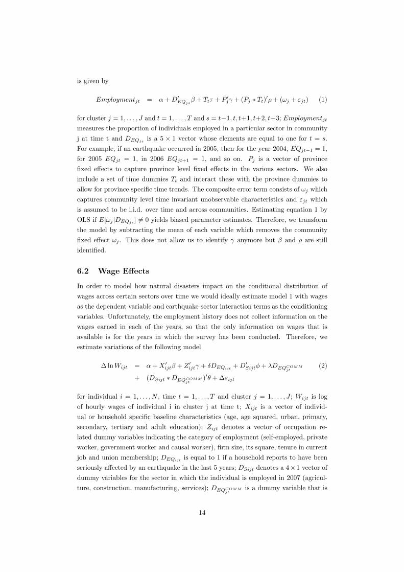
Figure 2 shows earthquakes with a magnitude larger than 5 on the Richter scale

in the region from the beginning of 1988 until February 2008. Colored circles indicate

earthquakes with a magnitude of at least 7.7 and aftershocks within the following 31

days. The green symbol denotes earthquakes for which fatalities were listed in the

Preliminary Determination of Epicenters publication of the U.S. Geological Survey.

From this map it is clear that earthquakes can happen anywhere in Sumatra and Java

and can thus be treated as random, therefore, it is not possible to predict a priori

where the next earthquake is going to happen.

5 Data

We combine two sources of data. First, we use household and community level data

from the Indonesia Family Life survey, a large-scale panel household survey conducted

in 1993, 1997, 2000 and 2007. In this study we only use data for males aged 15-

65 and for the last two rounds, since the retrospective disaster module was only

collected in the 2007 round, and further, including the previous years would make it

far more difficult to disentangle the effect of natural disasters from the effects of the

9

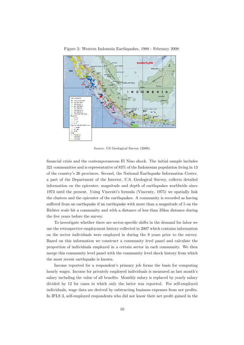
Figure 2: Western Indonesia Earthquakes, 1988 - February 2008

Source: US Geological Survey (2008).

financial crisis and the contemporaneous El Nino shock. The initial sample includes

321 communities and is representative of 83% of the Indonesian population living in 13

of the country’s 26 provinces. Second, the National Earthquake Information Center,

a part of the Department of the Interior, U.S. Geological Survey, collects detailed

information on the epicenter, magnitude and depth of earthquakes worldwide since

1973 until the present. Using Vincenti’s formula (Vincenty, 1975) we spatially link

the clusters and the epicenter of the earthquakes. A community is recorded as having

suffered from an earthquake if an earthquake with more than a magnitude of 5 on the

Richter scale hit a community and with a distance of less than 35km distance during

the five years before the survey.

To investigate whether there are sector-specific shifts in the demand for labor we

use the retrospective employment history collected in 2007 which contains information

on the sector individuals were employed in during the 9 years prior to the survey.

Based on this information we construct a community level panel and calculate the

proportion of individuals employed in a certain sector in each community. We then

merge this community level panel with the community level shock history from which

the most recent earthquake is known.

Income reported for a respondent’s primary job forms the basis for computing

hourly wages. Income for privately employed individuals is measured as last month’s

salary including the value of all benefits. Monthly salary is replaced by yearly salary

divided by 12 for cases in which only the latter was reported. For self-employed

individuals, wage data are derived by subtracting business expenses from net profits.

In IFLS 3, self-employed respondents who did not know their net profit gained in the

10

last month were further asked for their gross income gained during the last month.

Although this would allow us to get income data for these individuals, as this question

is dropped in IFLS 4, for comparability we drop observations who reported zero profit

in either of the rounds.

Following (Strauss, Beegle, Dwiyanto, Herawati, Pattinasarany, Satriawan, Sikoki,

Sukamdi, and Witoelar, 2004), we compute hourly wages on the basis of monthly re-

ported earnings divided by the total hours worked last week multiplied by 4.33. We

top code individuals who reported working more than a total of 126 hours per week

to 126 (assuming a maximum work load of 18 hours per day for 7 days a week) and

only include individuals with positive earnings in both years 7.

Following Thomas, Frankenberg, and Teruel (1999), we deflate 2007 and 2000

wages to the base year 1996 using a province-specific price deflator that is based

on the BPS price indices reported for 45 cities in Indonesia (43 cities until 2003),

matching the BPS cities to the IFLS provinces and using a simple average of the

price indices for provinces with more than one city8.

Table 1: Summary statisticsVariable Mean Std. Dev. N

Age 36.829 10.876 2770Primary Education 0.456 0.498 2770Secondary Education 0.403 0.491 2770Tertiary Education 0.094 0.292 2770Urban 0.536 0.499 2770Earthquake 0.054 0.226 2770Earthquake Community 0.201 0.401 2770Agriculture 0.271 0.445 2770Construction 0.161 0.368 2770Manufacturing 0.098 0.297 2770Services 0.47 0.499 2770

Table 1 presents some basic descriptive statistics of the sample in 2007. The

average age is almost 37 years. 46% of the respondents have primary education, and

about 40% have secondary education. About 9% has tertiary education. Slightly

more than half of the sample lives in urban communities. 5.4% of individuals reports

an earthquake in the area in which they live that was ’severe enough to cause death or

major injuries of a household member, direct financial loss to the household, or cause

household members to relocate’. About 20% of the communities report an earthquake.

With regards to employment, 27% of individuals are employed in agriculture, 16% in

construction, 9% in manufacturing and 47% in services.

7Strauss, Beegle, Dwiyanto, Herawati, Pattinasarany, Satriawan, Sikoki, Sukamdi, and Witoelar(2004) bottom code individuals with zero wage to rp30/hour.

8Thomas, Frankenberg, and Teruel (1999) construct an alternative measure for inflation basedon the price data collected in the IFLS community questionnaire and find that rural inflation was5% higher than urban inflation; therefore, they decide to further inflate prices for rural residents.Given that the period between 2000 and 2007 has noted a far more stable price environment thanpre-crisis, we only use the BPS price data. As will be explicit in the next section which outlines theempirical framework, we take first differences to account for location specific time invariant effects;further, we include a dummy variable if the household lives in an urban area as well as communityfixed effects to allow for differential wage growth in urban centers and for each of the communities.

11

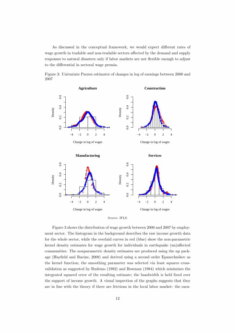
As discussed in the conceptual framework, we would expect different rates of

wage growth in tradable and non-tradable sectors affected by the demand and supply

responses to natural disasters only if labor markets are not flexible enough to adjust

to the differential in sectoral wage premia.

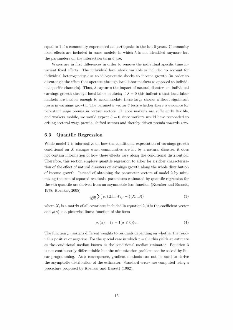
Figure 3: Univariate Parzen estimator of changes in log of earnings between 2000 and2007

Agriculture

Change in log of wages

Den

sity

−4 −2 0 2 4

0.0

0.2

0.4

0.6

Construction

Change in log of wages

Den

sity

−4 −2 0 2 4

0.0

0.2

0.4

0.6

Manufacturing

Change in log of wages

Den

sity

−4 −2 0 2 4

0.0

0.2

0.4

0.6

Services

Change in log of wages

Den

sity

−4 −2 0 2 4

0.0

0.2

0.4

0.6

Source: IFLS.

Figure 3 shows the distribution of wage growth between 2000 and 2007 by employ-

ment sector. The histogram in the background describes the raw income growth data

for the whole sector, while the overlaid curves in red (blue) show the non-parametric

kernel density estimates for wage growth for individuals in earthquake (un)affected

communities. The nonparametric density estimates are produced using the np pack-

age (Hayfield and Racine, 2008) and derived using a second order Epanechnikov as

the kernel function; the smoothing parameter was selected via least squares cross-

validation as suggested by Rudemo (1982) and Bowman (1984) which minimizes the

integrated squared error of the resulting estimate; the bandwidth is held fixed over

the support of income growth. A visual inspection of the graphs suggests that they

are in line with the theory if there are frictions in the local labor market: the earn-

12

ings growth distribution of individuals employed in non-tradable sectors (construction

and services) is shifted to the right for individuals who live in communities that were

affected by earthquakes. Manufacturing and agriculture on the other hand, exhibit

a shift to the left and therefore slow-down in income growth for earthquake affected

communities.

We formally test the equality of the empirical probability density functions using

a univariate entropy density equality test as proposed by Maasoumi and Racine (2002)

with 99 bootstrap replications sampled from the pooled distribution. The test statistic

and p-value as reported in Table 2 suggest that the null of equality can be rejected for

the construction sector at the 10% level and for the agriculture and manufacturing

sector at the 5% level. For services, on the other hand, we fail to reject the null of

equality of the two probability density functions at the 10% level.

Table 2: Nonparametric Entropy Test for Univariate Density Equality (Maasoumiand Racine, 2002)

Sector Test Statistic P-valueAgriculture 0.021 0.010Construction 0.016 0.091Manufacturing 0.061 0.010Services 0.009 0.293

Having established that earthquakes do appear to affect the distribution of earn-

ings growth in the different sectors, we now examine in more detail the channels

through which these effects might operate.

6 Empirical Framework

We attempt to identify the effect of destructive natural disasters from a number of

angles: first, whether there is evidence for an expansion and contraction of certain

sectors in the aftermath of an earthquake. Second, we test whether labor markets are

sufficiently flexible to accommodate these demand shifts or whether are there long

lasting sectoral wage premia even after occupational mobility has taken place; we

finally explore whether natural disasters lead to pure location shifts of the income

growth distribution or changes of the shape of the income growth distribution and

discuss heterogeneity of impacts with regard to characteristics of the earthquake and

the role of migration.

6.1 Demand Effects

We use the 9-year community level panel to explore whether we observe an expan-

sion of employment in non-tradable sectors and a contraction in tradable sectors in

communities that were affected by an earthquake. Further, we investigate the time

structure of these sectoral shifts. The model to test whether there are demand effects

13

is given by

Employmentjt = α+D′EQjsβ + Ttτ + P ′jγ + (Pj ∗ Tt)′ρ+ (ωj + εjt) (1)

for cluster j = 1, . . . , J and t = 1, . . . , T and s = t−1, t, t+1, t+2, t+3; Employmentjt

measures the proportion of individuals employed in a particular sector in community

j at time t and DEQjsis a 5 × 1 vector whose elements are equal to one for t = s.

For example, if an earthquake occurred in 2005, then for the year 2004, EQjt−1 = 1,

for 2005 EQjt = 1, in 2006 EQjt+1 = 1, and so on. Pj is a vector of province

fixed effects to capture province level fixed effects in the various sectors. We also

include a set of time dummies Tt and interact these with the province dummies to

allow for province specific time trends. The composite error term consists of ωj which

captures community level time invariant unobservable characteristics and εjt which

is assumed to be i.i.d. over time and across communities. Estimating equation 1 by

OLS if E[ωj |DEQjs] 6= 0 yields biased parameter estimates. Therefore, we transform

the model by subtracting the mean of each variable which removes the community

fixed effect ωj . This does not allow us to identify γ anymore but β and ρ are still

identified.

6.2 Wage Effects

In order to model how natural disasters impact on the conditional distribution of

wages across certain sectors over time we would ideally estimate model 1 with wages

as the dependent variable and earthquake-sector interaction terms as the conditioning

variables. Unfortunately, the employment history does not collect information on the

wages earned in each of the years, so that the only information on wages that is

available is for the years in which the survey has been conducted. Therefore, we

estimate variations of the following model

∆ lnWijt = α+X ′ijtβ + Z ′ijtγ + δDEQijt+D′Sijtφ+ λDEQCOMM

jt(2)

+ (DSijt ∗DEQCOMMjt

)′θ + ∆εijt

for individual i = 1, . . . , N , time t = 1, . . . , T and cluster j = 1, . . . , J ; Wijt is log

of hourly wages of individual i in cluster j at time t; Xijt is a vector of individ-

ual or household specific baseline characteristics (age, age squared, urban, primary,

secondary, tertiary and adult education); Zijt denotes a vector of occupation re-

lated dummy variables indicating the category of employment (self-employed, private

worker, government worker and causal worker), firm size, its square, tenure in current

job and union membership; DEQijtis equal to 1 if a household reports to have been

seriously affected by an earthquake in the last 5 years; DSijt denotes a 4×1 vector of

dummy variables for the sector in which the individual is employed in 2007 (agricul-

ture, construction, manufacturing, services); DEQCOMMjt

is a dummy variable that is

14

equal to 1 if a community experienced an earthquake in the last 5 years. Community

fixed effects are included in some models, in which λ is not identified anymore but

the parameters on the interaction term θ are.

Wages are in first differences in order to remove the individual specific time in-

variant fixed effects. The individual level shock variable is included to account for

individual heterogeneity due to idiosyncratic shocks to income growth (in order to

disentangle the effect that operates through local labor markets as opposed to individ-

ual specific channels). Thus, λ captures the impact of natural disasters on individual

earnings growth through local labor markets; if λ = 0 this indicates that local labor

markets are flexible enough to accommodate these large shocks without significant

losses in earnings growth. The parameter vector θ tests whether there is evidence for

persistent wage premia in certain sectors. If labor markets are sufficiently flexible,

and workers mobile, we would expect θ = 0 since workers would have responded to

arising sectoral wage premia, shifted sectors and thereby driven premia towards zero.

6.3 Quantile Regression

While model 2 is informative on how the conditional expectation of earnings growth

conditional on X changes when communities are hit by a natural disaster, it does

not contain information of how these effects vary along the conditional distribution.

Therefore, this section employs quantile regression to allow for a richer characteriza-

tion of the effect of natural disasters on earnings growth along the whole distribution

of income growth. Instead of obtaining the parameter vectors of model 2 by mini-

mizing the sum of squared residuals, parameters estimated by quantile regression for

the τth quantile are derived from an asymmetric loss function (Koenker and Bassett,

1978; Koenker, 2005)

minβεR

∑ρτ (∆ lnWijt − ξ(Xi, β)) (3)

where Xi is a matrix of all covariates included in equation 2, β is the coefficient vector

and ρ(u) is a piecewise linear function of the form

ρτ (u) = (τ − 1(u 0 0))u. (4)

The function ρτ assigns different weights to residuals depending on whether the resid-

ual is positive or negative. For the special case in which τ = 0.5 this yields an estimate

at the conditional median known as the conditional median estimator. Equation 3

is not continuously differentiable but the minimization problem can be solved by lin-

ear programming. As a consequence, gradient methods can not be used to derive

the asymptotic distribution of the estimator. Standard errors are computed using a

procedure proposed by Koenker and Bassett (1982).

15

7 Discussion

This section discusses the results of the various empirical models outlined above,

starting with evidence on employment effects. We then explore wage effects and

present a number of robustness checks before characterizing these effects along the

whole income growth distribution. Finally, we discuss heterogeneity with regard to

the distance and magnitude of an earthquake and the role of migration in potentially

biasing our results.

7.1 Demand Effects

Tables 3 - 6 present the results for specification 1 which tests whether there are signifi-

cant shifts across employment sectors following an earthquake. As the random effects

estimates are virtually identical in size and significance, we only report fixed effects

estimates. Standard errors are corrected for correlation of errors for the same cluster

across time, as well as for non-constant variances on the diagonal of the variance

covariance matrix. The dependent variable is zero for clusters for which no individual

in the survey works in a particular sector, and we have estimated the above specifica-

tions including both zero and positive observations. Limiting the sample to positive

observations leaves the results virtually unchanged apart from slightly higher coef-

ficients which would be expected in since the presence of zeros biases the estimates

downwards. If the censoring would be due to a different data generating process for

zero and non-zero observations this would require models such as a generalized tobit

model that allow for either separate estimation or correlation between the errors of

the two parts of the model. However, as here the presence of zeros is most likely

due to sampling error, in the sense that no individuals working in a particular sector

with positive wages were sampled in both rounds, this does not appear to be a major

estimation issue.

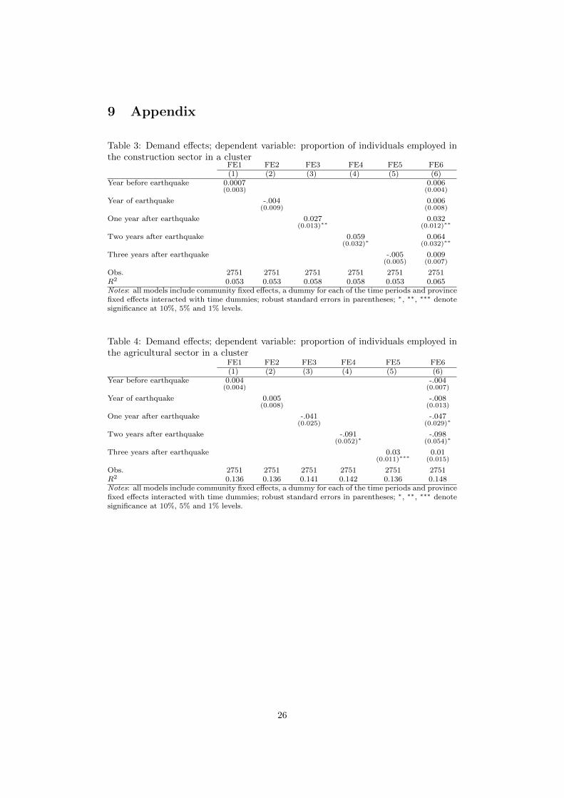
The results suggest that there is a significant 2.7% point increase in the proportion

of individuals employed in construction one year after the earthquake and a 5.9% point

increase two years following the earthquake 9. This effect is disappears again in the

third year after the earthquake. As one would expect, there are no effects for the year

prior to the earthquake as well as in the year the earthquake happens. The size and

significance of the coefficients is remarkably robust to the inclusion of fixed effects, as

well as to the joint inclusion of all the earthquake timing variables.

Table 4 illustrates that there is a matching contraction of the proportion of indi-

viduals working in the agricultural sector when a natural disaster hits a community.

In a fairly symmetric manner, the proportion of individuals working in agriculture one

year after an earthquake decreases by 4.1% points and 9.1% points two years after the

9We limited the sample to individuals who were residents in the same cluster in 2000 in order notto bias the estimate by in-migration of individuals into the IFLS households. If we use the wholesample regardless of where individuals resided in 2000, the effect for one year after the earthquakestays the same but for 2 years after the earthquake becomes insignificant.

16

earthquake. There appears to be a shift back into the agriculture sector 3 years after

an earthquake took place, but this effect is not robust to the inclusion of the whole

set of time dummies in column (6) where similar to the construction sector, the effect

vanishes in the third year after an earthquake took place. From this it appears that

we observe a natural disasters push residents in a community from agriculture-based

activities into the construction sector which is consistent with what the theoretical

framework would predict at least for the agriculture and constructions sector. Hav-

ing established that there are significant labor demand effects in earthquake affected

communities, we now investigate whether labor markets are sufficiently flexible to

accommodate these shifts.

7.2 Wage Effects

Table 7 presents the results of specification 2, which suggest that individuals’ earnings

bounce back after earthquakes as there is no evidence that the household-reported

earthquake affects income growth after controlling for socio-economic variables, cat-

egory of employment and occupational sector. Further, the coefficient on the com-

munity level earthquake shock is not significantly different from zero, indicating that

there is no evidence that earthquakes impact on wage growth through local labor

markets on average. However, when adding the sector-shock interaction terms, the

coefficient on the community level earthquake shock becomes negative, although in-

significant, suggesting that heterogeneity of impacts was upward biasing the coefficient

towards zero in column (1). This bias stems from a significant and positive effect for

individuals who live in a community that was affected by an earthquake, if they are

employed in construction. Their wage growth was 60% higher compared to individ-

uals employed in agriculture, while there is no effect for individuals employed in the

manufacturing or service sector. The effect is robust to the inclusion of community

fixed effects to account for community level heterogeneity such as differences in labor

market integration and wage levels. This indicates that even after individuals have

responded to to changes in local labor market conditions (which would drive down

wage premia and thereby bias the estimate of θ towards zero), there are still significant

and positive wage premia for individuals employed in construction.

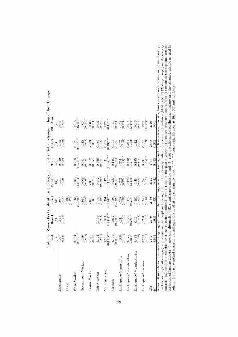
7.3 Robustness Checks

This section reports the results of a number of robustness checks of specification 2,

including different sets of controls, using USGS earthquake data as an alternative

measure for the reported earthquake incidence, inclusion of other shock variables,

province fixed effects, a trimmed sample and instrumenting for the earthquake variable

using the USGS measure for earthquake incidence. As the coefficients do not change

substantially when community fixed effects are included, and we would also like to

inspect the stability of the coefficient on the community level earthquake shock (which

17

is not identified anymore under the community fixed effects specification), we use

column (3) of Table 7 as the base model which is reported in column (1) of Table 8.

If individuals’ entrepreneurial talent changes over time and in response to an

earthquake they enter the construction sector and start up firms there, then higher

wage growth in the construction sector operates through unobserved changes in talent

and shifts in employment categories rather than sectoral wage premia. Column (2)

therefore drops the employment category variables which leaves the coefficient on the

sector-shock interaction terms unaffected. Column (3) then adds the second most

frequently reported natural disaster, floods, as an additional control to account for

individual level heterogeneity in earnings. It is excluded in the base model due to

concerns that floods are not exogenous as the location of a household which makes

it more or less vulnerable to floods (i.e. next to rivers) is most likely correlated with

other unobservable determinants of earnings growth. The results remain robust to its

inclusion. Column (4) includes province fixed effects which also does not change the

parameter estimates. Column (5) presents a trimmed sample which excludes the top

and bottom one percentile of income growth which implies excluding 54 individuals.

The size of the coefficient is stable when excluding outliers from the sample and

increases in significance, with a significant effect now also for the services sector.

Column (6) uses an alternative measure of earthquakes, from the US Geological Survey

instead of the community level reported earthquake shock and column (7) uses the

same measure on the trimmed sample used in column (5). As the measure constructed

using data from the US Geological Survey is significantly more noisy than the reported

earthquake measure from the IFLS questionnaire, standard errors on the coefficient

of the sector-shock interaction terms are larger. However, when we use the trimmed

sample in column (7) standard errors are smaller again. The coefficients are also

fairly stable in size across the various specifications. Having established a robust and

significant effect of earthquakes on wage growth in different sectors, we now explore

whether these effects occur at certain parts of the income distribution or along the

whole distribution by using quantile regression.

7.4 Quantile Regression

Table 9 shows the estimated quantile coefficients on the sector variables and the

sector-shock interaction terms. Due to the symmetry of the distribution of the log

of income growth, the coefficients for the 0.5 quantile, the median, are very similar

to the conditional mean estimates. The results reveal that the positive sectoral wage

premia in construction, manufacturing and services apparent from the least squares

estimates are mainly driven by higher wage growth for individuals at the lower half of

the income growth distribution. Further, the size of the coefficient on the earthquake-

sector interaction term tends to increase in size and significance at higher quantiles,

a feature that OLS estimates do not reveal. Further, column (7) reveals that while

the coefficient on the service sector-shock interaction term is never statistically sig-

18

nificantly different from zero in the OLS estimates (apart from column (5) and (7) in

Table 8 that use the trimmed sample), the quantile regression results show that there

are significant and positive effects at the middle of the distribution and then again at

the top also for the service sector. As quantile regression is less sensitive to outliers it

allows us to recover this effect using the full sample; in the least squares regressions

the significant effect for the service sector only appeared when we used the trimmed

sample. This confirms that there are significant increases in wage growth for both sec-

tors producing non-tradable goods, namely, the construction and the service sector,

compared to tradable sectors such as agriculture (the base group) and manufacturing

(for which there is no effect along the whole distribution).

Figure 9 graphically illustrates the results of the quantile regression over the

whole income growth distribution. The x-axis marks the quantiles of the income

growth distribution and the y-axis the size of the estimated coefficient with a reference

line in cranberry at zero. The solid line shows the coefficient estimated by quantile

regression with a 90% confidence band marked by the grey area. The dashed line

represents the least squares estimate with a 90% confidence interval indicated by

the dotted line. For both the employment category and the occupational sector, the

quantile regression estimates lie outside the confidence interval of the least squares

estimates, in particular at the high and low end of the distribution. Government

workers and Casual workers appear to have had significantly higher income growth

at the low levels of the income growth distribution compared to the self-employed.

Among individuals not living in an earthquake affected community, those at the

lower half of the income growth distribution experienced higher growth when em-

ployed in construction, manufacturing or services compared to agriculture. On the

other hand, for individuals who saw their income increase by more than the increase

of the median, they experienced negative sectoral effects if employed in construction

and manufacturing, where the quantile regression estimates are below the zero line

and outside the least squares estimates. In other words, those who saw mild increases

in income, still benefitted from being employed in any sector other than agriculture,

while for those with large increases in income, there are negative returns to being em-

ployed in a non-agricultural sector. Interestingly, the bottom three panels show that

earthquakes seem to neutralize the differential earnings growth patterns across sec-

tors; the effect of being employed in the construction sector in an earthquake affected

community is fairly constant along the income distribution, indicating that earth-

quakes exert a pure location shift rather than altering the shape of the conditional

distribution. The graphs illustrate again that individuals employed in the services

sector with wage growth between the 0.4 and 0.6 quantile experienced significantly

higher wage growth if they were living in an earthquake affected community which

is where the confidence band of the quantile regression does not include zero. For

all three sector-shock interaction terms, the coefficients estimated by quantile regres-

sion lie within the confidence intervals for the least squares estimates over almost the

19

whole range of the income growth distribution, suggesting that the interaction effects

are fairly constant across the conditional distribution of the independent variable.

7.5 Distance to the Epicenter and Magnitude

Unfortunately the community questionnaire does not provide information on the mag-

nitude of the earthquake and the distance to the epicenter. We have tried to backward

construct these two variables by searching for earthquakes in the USGS database that

happened in the year in which the community reported an earthquake within a ra-

dius of 90km. We then included the largest magnitude and smallest distance that

was recorded for earthquakes in a particular year for a particular community. The

coefficients on both variables are not significantly different from zero. Further, the

other results remain unchanged, in both size and significance level of the coefficients,

except that the coefficient on the earthquake-sector interaction term in table 8 is sig-

nificant at the 11% level instead of the 10% level. Since it adds additional noise, and

decreases the sample slightly as for some earthquakes the information on the year of

the earthquake is missing, we decided to report the results without these additional

controls.

7.6 Migration

One concern is that natural disasters lead to large flows of migration. It could be

that those with intact safety nets manage to stay in a community, and those without

are forced to migrate. On the other hand, it might be that migrating households

are those who are less liquidity constrained or have better connections in other lo-

cations. Therefore, it is not clear in which direction the bias goes. In the migration

section of the questionnaire the three most frequently stated reasons for migration are

work-related migration (34%), marriage (15%) and education (11%); only 0.33% of

individuals give natural disasters as a reason for migration. However, while providing

some evidence, one would worry that natural disasters nevertheless play an important

role in affecting an individual’s migration decision but the ultimate reason given will

still be to find work or be closer to the family. For example, for an individual in an

area that has frequently been hit by an earthquake or a flood, an individual migrating

might still give work as the reason for migration although clearly the lack of work in

the home location is not uncorrelated with the event of a natural disaster. Therefore,

we explore whether there is any significant link in the data between migration and

the event of an earthquake. We construct a number of variables to measure migra-

tion flows: the proportion of a household who migrated between 2000 and 2007, the

number of household members who migrated between 2000 and 2007, and the change

in the number of migrants in a household between 1997 and 2000, and 2000 and

2007. Regressing these migration measures on the earthquake variable, controlling

for province fixed effects and urban/rural location, a linear model, an ordered probit

20

and a probit model do not show any evidence for a significant relationship between

the propensity to migrate and the event of an earthquake. Therefore, the local econ-

omy appears to be fairly insulated and the population remaining after an earthquake

representative.

8 Conclusion and Next Steps

This paper studies how local labor markets adjust to destructive natural disasters, in

particular the change in the relative price of tradable to non-tradable goods induced

by the increase in the demand for construction as well as the inflow of resources in the

aftermath of natural disasters. To our knowledge, this is the first study that explores

the impact of destructive natural disasters on local labor markets in the context of a

low or low to middle income country.

Our results are in line with the predictions coming out of the theoretical frame-

work and suggest that there are important general equilibrium effects, such as a

reallocation of employment and wage premia between sectors producing tradable vs

non-tradable goods. First, using a community-level panel we establish that there are

significant shifts in the demand for labor from the agriculture sector into the construc-

tion sector in the two years following an earthquake. Second, we find that individuals

employed in non-tradable sectors in earthquake affected communities experience sig-

nificant and positive wage premia which persist even after mobility has taken place,

suggesting that local labor markets exhibit a fairly high degree of rigidity. These

effects are homogenous along the quantiles of the conditional income growth distribu-

tion. Thereby, they neutralize otherwise arising differential earnings growth patterns

across sectors and operate as pure location shifts of the income distribution than al-

tering the shape. As a next step we want to further investigate the channels through

which these persistent wage effects occur, in particular infrastructure destruction and

changes in the relative prices of goods.

21

References

Baez, J., and I. Santos (2008): “On Shaky Ground: The Effects of Earthquakes

on Household Income and Poverty,” .

Banerjee, L. (2007): “Effect of Flood on Agricultural Wages in Bangladesh: An

Empirical Analysis,” World Development, 35(11), 1989–2009.

BAPPENAS (2006): “Preliminary Damage and Loss Assessment: Yogyakarta and

Central Java Natural Disaster,” .

Belasen, A. R., and S. Polachek (2009): “How Disasters Affect Local Labor

Markets: The Effects of Hurricanes in Florida,” Journal of Human Resources, 44(1),

251.

Belasen, A. R., and S. W. Polachek (2008): “How Hurricanes Affect Wages and

Employment in Local Labor Markets,” American Economic Review, 98(2), 49–53.

Benson, C., and E. Clay (2004): Understanding the economic and financial impacts

of natural disasters. World Bank Publications.

BNPB et al (2009): “West Sumatra and Jambi Natural Disasters: Damage, Loss

and Preliminary Needs Assessment,” Joint report by the BNPB, Bappenas, and

the Provincial and District/City Governments of West Sumatra and Jambi and

international partners.

Bowman, A. (1984): “An alternative method of cross-validation for the smoothing

of density estimates,” Biometrika, 71(2), 353.

Cameron, L., and C. Worswick (2003): “The labor market as a smoothing device:

labor supply responses to crop loss,” Review of Development Economics, 7(2), 327–

341.

Carrington, W. (1996): “The Alaskan labor market during the pipeline era,” Jour-

nal of Political Economy, 104(1), 186–218.

Cavallo, E., and I. Noy (2009): “The Economics of Natural Disasters - A Survey,”

Working Papers 200919, University of Hawaii at Manoa, Department of Economics.

Collier, P., and J. Gunning (1999): Trade Shocks in Developing Countries:

Africa. Oxford University Press, USA.

Corden, W. (1984): “Booming sector and Dutch disease economics: survey and

consolidation,” Oxford Economic Papers, 36(3), 359–380.

Corden, W., and P. Neary (1982): “Booming Sector and De-Industrialization in

a Small Open Economy,” Economic Journal, 92, 368.

22

Cuaresma, C., Hlouskova, and Obersteiner (2008): “Natural Disasters As

Creative Destruction? Evidence From Developing Countries,” Economic Inquiry,

46(2), 214–226.

Datt, G., and H. Hoogeveen (2003): “El Nino or El Peso? Crisis, poverty and

income distribution in the Philippines,” World Development, 31(7), 1103–1124.

Dercon, S. (2004): “Growth and shocks: evidence from rural Ethiopia,” Journal of

Development Economics, 74(2), 309–329.

Government of Haiti et al (2010): “Haiti Earthquake PDNA: Assessment of

damage, losses, general and sectoral needs, Annex to the Action Plan for National

Recovery and Development of Haiti,” Working paper prepared by the Government

of Haiti with support from the International Community.

Halliday, T. (2006): “Migration, Risk, and Liquidity Constraints in El Salvador,”

Economic Development and Cultural Change, 54(4), 893–925.

Hayfield, T., and J. S. Racine (2008): “Nonparametric Econometrics: The np

Package,” Journal of Statistical Software, 27(5), 1–32.

Hochrainer, S. (2009): “Assessing The Macroeconomic Impacts Of Natural Disas-

ters,” Policy Research Working Paper 4968, World Bank.

Jayachandran, S. (2006): “Selling Labor Low: Wage Responses to Productivity

Shocks in Developing Countries,” Journal of Political Economy, 114(3), 538–575.

Keane, M., and E. Prasad (1996): “The employment and wage effects of oil price

changes: a sectoral analysis,” The Review of Economics and Statistics, 78(3), 389–

400.

Kline, P. (2008): “Understanding Sectoral Labor Market Dynamics: An Equilibrium

Analysis of the Oil and Gas Field Services Industry,” .

Kochar, A. (1999): “Smoothing consumption by smoothing income: hours-of-work

responses to idiosyncratic agricultural shocks in rural India,” Review of Economics

and Statistics, 81(1), 50–61.

Koenker, R. (2005): Quantile regression. Cambridge University Press.

Koenker, R., and J. Bassett, Gilbert (1978): “Regression Quantiles,” Econo-

metrica, 46(1), 33–50.

Koenker, R., and J. Bassett, Gilbert (1982): “Robust Tests for Heteroscedas-

ticity Based on Regression Quantiles,” Econometrica, 50(1), 43–61.

Loayza, N., E. Olaberrıa, J. Rigolini, and L. Christiaensen (2009): “Natural

Disasters and Growth,” Discussion paper.

23

Maasoumi, E., and J. Racine (2002): “Entropy and predictability of stock market

returns,” Journal of Econometrics, 107(1-2), 291–312.

McIntosh, M. F. (2008): “Measuring the Labor Market Impacts of Hurricane Ka-

trina Migration: Evidence from Houston, Texas,” American Economic Review,

98(2), 54–57.

Moretti, E. (2010a): “Local Labor Markets,” Handbook of Labor Economics, forth-

coming.

(2010b): “Local Multipliers,” American Economic Review, 100(2), 373–77.

Mueller, V., and D. Osgood (2009): “Long-term Impacts of Droughts on Labour

Markets in Developing Countries: Evidence from Brazil,” Journal of Development

Studies, 45(10), 1651–1662.

Mueller, V., and A. Quisumbing (2010): “Short- and long-term effects of the

1998 Bangladesh flood on rural wages,” Discussion paper.

Noy, I. (2009): “The macroeconomic consequences of disasters,” Journal of Devel-

opment Economics, 88(2), 221–231.

Paxson, C. H. (1992): “Using Weather Variability to Estimate the Response of

Savings to Transitory Income in Thailand,” American Economic Review, 82(1),

15–33.

Premand, P. (2008): “Hurricane Mitch and consumption growth of Nicaraguan

agricultural households,” The Centre for the Study of African Economies Working

Paper.

Rose, E. (2001): “Ex ante and ex post labor supply response to risk in a low-income

area,” Journal of Development Economics, 64(2), 371–388.

Rudemo, M. (1982): “Empirical choice of histograms and kernel density estimators,”

Scandinavian Journal of Statistics, 9(2), 65–78.

Silva, D. G. D., R. P. McComb, Y.-K. Moh, A. R. Schiller, and A. J. Vargas

(2010): “The Effect of Migration on Wages: Evidence from a Natural Experiment,”

American Economic Review, 100(2), 321–26.

Skidmore, M., and H. Toya (2002): “Do natural disasters promote long-run

growth?,” Economic Inquiry, 40(4), 664–687.

Strauss, J., K. Beegle, A. Dwiyanto, Y. Herawati, D. Pattinasarany,

E. Satriawan, B. Sikoki, B. Sukamdi, and F. Witoelar (2004): Indonesian

living standards three years after the crisis: evidence from the Indonesia Family

Life Survey. RAND Corporation.

24

Strobl, E. (2010): “The economic growth impact of hurricanes: evidence from US

coastal counties,” The Review of Economics and Statistics,forthcoming.

Stromberg, D. (2007): “Natural Disasters, Economic Development, and Humani-

tarian Aid,” Journal of Economic Perspectives, 21(3), 199–222.

Takasaki, Y., B. L. Barham, and O. T. Coomes (2010): “Smoothing Income

against Crop Flood Losses in Amazonia: Rain Forest or Rivers as a Safety Net?,”

Review of Development Economics, 14(1), 48–63.

Thomas, D., K. Frankenberg, E.and Beegle, and G. Teruel (1999): “House-

hold budgets, household composition and the crisis in Indonesia: evidence from

longitudinal household survey data,” Mimeo.

Townsend, R. M. (1994): “Risk and Insurance in Village India,” Econometrica,

62(3), 539–91.

Udry, C. (1995): “Risk and Saving in Northern Nigeria,” American Economic Re-

view, 85(5), 1287–1300.

US Geological Survey (2008): “Seismic Hazard of Western Indonesia,” National

Earthquake Information Center.

Van den Berg, M. (2010): “Household income strategies and natural disasters:

Dynamic livelihoods in rural Nicaragua,” Ecological Economics, 69(3), 592–602.

Vincenty, T. (1975): “Direct and inverse solutions of geodesics on the ellipsoid with

application of nested equations,” Survey review, 23(176), 88–93.

World Bank (2008): “Aceh Tsunami Reconstruction Expenditure Tracking Up-

date,” .

Yang, D. (2008): “Risk, Migration, and Rural Financial Markets: Evidence from

Earthquakes in El Salvador,” Social Research: An International Quarterly, 75(3),

955–992.

25

9 Appendix

Table 3: Demand effects; dependent variable: proportion of individuals employed inthe construction sector in a cluster

FE1 FE2 FE3 FE4 FE5 FE6(1) (2) (3) (4) (5) (6)

Year before earthquake 0.0007 0.006(0.003) (0.004)

Year of earthquake -.004 0.006(0.009) (0.008)

One year after earthquake 0.027 0.032(0.013)∗∗ (0.012)∗∗

Two years after earthquake 0.059 0.064(0.032)∗ (0.032)∗∗

Three years after earthquake -.005 0.009(0.005) (0.007)

Obs. 2751 2751 2751 2751 2751 2751R2 0.053 0.053 0.058 0.058 0.053 0.065Notes: all models include community fixed effects, a dummy for each of the time periods and provincefixed effects interacted with time dummies; robust standard errors in parentheses; ∗, ∗∗, ∗∗∗ denotesignificance at 10%, 5% and 1% levels.

Table 4: Demand effects; dependent variable: proportion of individuals employed inthe agricultural sector in a cluster

FE1 FE2 FE3 FE4 FE5 FE6(1) (2) (3) (4) (5) (6)

Year before earthquake 0.004 -.004(0.004) (0.007)

Year of earthquake 0.005 -.008(0.008) (0.013)

One year after earthquake -.041 -.047(0.025) (0.029)∗

Two years after earthquake -.091 -.098(0.052)∗ (0.054)∗

Three years after earthquake 0.03 0.01(0.011)∗∗∗ (0.015)

Obs. 2751 2751 2751 2751 2751 2751R2 0.136 0.136 0.141 0.142 0.136 0.148Notes: all models include community fixed effects, a dummy for each of the time periods and provincefixed effects interacted with time dummies; robust standard errors in parentheses; ∗, ∗∗, ∗∗∗ denotesignificance at 10%, 5% and 1% levels.

26

Table 5: Demand effects; dependent variable: proportion of individuals employed inthe manufacturing sector in a cluster

FE1 FE2 FE3 FE4 FE5 FE6(1) (2) (3) (4) (5) (6)

Year before earthquake 0.0009 0.007(0.004) (0.008)

Year of earthquake 0.005 0.014(0.008) (0.013)

One year after earthquake 0.025 0.031(0.019) (0.023)

Two years after earthquake -.017 -.011(0.014) (0.015)

Three years after earthquake -.008 -.002(0.009) (0.011)

Obs. 2751 2751 2751 2751 2751 2751R2 0.066 0.066 0.068 0.066 0.066 0.069Notes: all models include community fixed effects, a dummy for each of the time periods and provincefixed effects interacted with time dummies; robust standard errors in parentheses; ∗, ∗∗, ∗∗∗ denotesignificance at 10%, 5% and 1% levels.

Table 6: Demand effects; dependent variable: proportion of individuals employed inthe services sector in a cluster

FE1 FE2 FE3 FE4 FE5 FE6(1) (2) (3) (4) (5) (6)

Year before earthquake -.006 -.009(0.005) (0.008)

Year of earthquake -.006 -.011(0.008) (0.012)

One year after earthquake -.011 -.015(0.017) (0.021)

Two years after earthquake 0.05 0.045(0.033) (0.034)

Three years after earthquake -.018 -.017(0.015) (0.017)

Obs. 2751 2751 2751 2751 2751 2751R2 0.183 0.183 0.183 0.184 0.183 0.184Notes: all models include community fixed effects, a dummy for each of the time periods and provincefixed effects interacted with time dummies; robust standard errors in parentheses; ∗, ∗∗, ∗∗∗ denotesignificance at 10%, 5% and 1% levels.

27

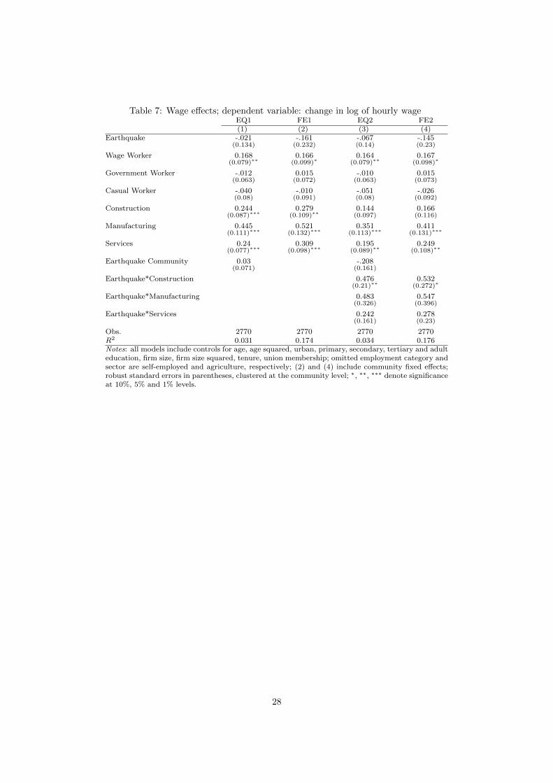
Table 7: Wage effects; dependent variable: change in log of hourly wageEQ1 FE1 EQ2 FE2(1) (2) (3) (4)

Earthquake -.021 -.161 -.067 -.145(0.134) (0.232) (0.14) (0.23)

Wage Worker 0.168 0.166 0.164 0.167(0.079)∗∗ (0.099)∗ (0.079)∗∗ (0.098)∗

Government Worker -.012 0.015 -.010 0.015(0.063) (0.072) (0.063) (0.073)

Casual Worker -.040 -.010 -.051 -.026(0.08) (0.091) (0.08) (0.092)

Construction 0.244 0.279 0.144 0.166(0.087)∗∗∗ (0.109)∗∗ (0.097) (0.116)

Manufacturing 0.445 0.521 0.351 0.411(0.111)∗∗∗ (0.132)∗∗∗ (0.113)∗∗∗ (0.131)∗∗∗

Services 0.24 0.309 0.195 0.249(0.077)∗∗∗ (0.098)∗∗∗ (0.089)∗∗ (0.108)∗∗

Earthquake Community 0.03 -.208(0.071) (0.161)

Earthquake*Construction 0.476 0.532(0.21)∗∗ (0.272)∗

Earthquake*Manufacturing 0.483 0.547(0.326) (0.396)

Earthquake*Services 0.242 0.278(0.161) (0.23)

Obs. 2770 2770 2770 2770R2 0.031 0.174 0.034 0.176Notes: all models include controls for age, age squared, urban, primary, secondary, tertiary and adulteducation, firm size, firm size squared, tenure, union membership; omitted employment category andsector are self-employed and agriculture, respectively; (2) and (4) include community fixed effects;robust standard errors in parentheses, clustered at the community level; ∗, ∗∗, ∗∗∗ denote significanceat 10%, 5% and 1% levels.

28

Tab

le8:

Wag

eeff

ects

rob

ust

nes

sch

ecks;

dep

end

ent

vari

ab

le:

change

inlo

gof

hou

rly

wage

Base

IB

ase

IIF

lood

Pro

vF

ET

rim

US

GS

US

GS

Tri

m(1

)(2

)(3

)(4

)(5

)(6

)(7

)E

art

hqu

ake

-.067

-.078

-.067

-.110

0.0

49

-.053

0.0

45

(0.14)

(0.138)

(0.14)

(0.2)

(0.09)

(0.142)

(0.09)

Flo

od

0.0

09

(0.079)

Wage

Work

er0.1

64

0.1

64

0.1

65

0.2

18

0.1

69

0.2

18

(0.079)∗

∗(0

.079)∗

∗(0

.081)∗

∗(0

.072)∗

∗∗

(0.078)∗

∗(0

.071)∗

∗∗

Gover

nm

ent

Work

er-.

010

-.010

0.0

08

0.0

41

-.015

0.0

3(0

.063)

(0.063)

(0.063)

(0.057)

(0.063)

(0.056)

Casu

al

Work

er-.

051

-.051

-.019

0.0

12

-.049

0.0

09

(0.08)

(0.08)

(0.078)

(0.069)

(0.081)

(0.071)

Con

stru

ctio

n0.1

44

0.1

36

0.1

45

0.1

72

0.0

66

0.1

89

0.0

87

(0.097)

(0.098)

(0.097)

(0.099)∗

(0.084)

(0.113)∗

(0.094)

Manu

fact

uri

ng

0.3

51

0.3

44

0.3

51

0.4

20.3

0.4

43

0.3

24

(0.113)∗

∗∗

(0.111)∗

∗∗

(0.114)∗

∗∗

(0.115)∗

∗∗

(0.097)∗

∗∗

(0.13)∗

∗∗

(0.1)∗

∗∗

Ser

vic

es0.1

95

0.2

12

0.1

94

0.2

37

0.1

35

0.1

93

0.1

1(0

.089)∗

∗(0

.088)∗

∗(0

.089)∗

∗(0

.091)∗

∗∗

(0.074)∗

(0.101)∗

(0.081)

Eart

hqu

ake

Com

mu

nit

y-.

208

-.211

-.208

-.224

-.251

-.052

-.152

(0.161)

(0.161)

(0.161)

(0.172)

(0.123)∗

∗(0

.148)

(0.121)

Eart

hqu

ake*

Con

stru

ctio

n0.4

76

0.4

75

0.4

76

0.4

76

0.4

92

0.2

11

0.2

11

(0.21)∗

∗(0

.209)∗

∗(0

.21)∗

∗(0

.217)∗

∗(0

.17)∗

∗∗

(0.163)

(0.147)∗

∗

Eart

hqu

ake*

Manu

fact

uri

ng

0.4

83

0.4

90.4

84

0.4

50.1

95

-.012

0.0

16

(0.326)

(0.326)

(0.326)

(0.333)

(0.179)

(0.231)

(0.172)

Eart

hqu

ake*

Ser

vic

es0.2

42

0.2

54

0.2

43

0.2

40.2

91

0.1

67

0.2

71

(0.161)

(0.161)

(0.161)

(0.17)

(0.135)∗

∗(0

.139)

(0.127)∗

∗

Ob

s.2770

2770

2770

2770

2716

2770

2716

R2

0.0

34

0.0

33

0.0

34

0.0

42

0.0

43

0.0

32

0.0

43

Notes:

all

mod

els

incl

ud

eco

ntr

ols

for

age,

age

squ

are

d,

urb

an

,p

rim

ary

,se

con

dary

,te

rtia

ryan

dad

ult

edu

cati

on

,fi

rmsi

ze,

firm

size

squ

are

d,

tenu

re,

un

ion

mem

ber

ship

;om

itte

dem

plo

ym

ent

cate

gory

an

dse

ctor

are

self

-em

plo

yed

an

dagri

cult

ure

,re

spec

tivel

y;

colu

mn

(1)

rep

rod

uce

sco

lum

n(3

)of

Tab

le7;

(2)

dro

ps

emp

loym

ent

cate

gory

contr

ols

;(3

)in

clu

des

avari

ab

lefo

rif

the

hou

seh

old

suff

ered

from

afl

ood

inth

ep

ast

5yea

rs;

(4)

incl

ud

esp

rovin

cefi

xed

effec

ts;

(5)

excl

ud

esth

eto

pan

db

ott

om

per

centi

leof

inco

me

gro

wth

(6)

use

sth

ealt

ern

ati

ve

US

GS

eart

hqu

ake

mea

sure

an

d(7

)u

ses

the

alt

ern

ati

ve

eart

hqu

ake

mea

sure

an

dth

etr

imm

edsa

mp

leas

use

din

colu

mn

5;

rob

ust

stan

dard

erro

rsin

pare

nth

eses

,cl

ust

ered

at

the

com

mu

nit

yle

vel

;∗,∗∗

,∗∗

∗d

enote

sign

ifica

nce

at

10%

,5%

an

d1%

level

s.

29

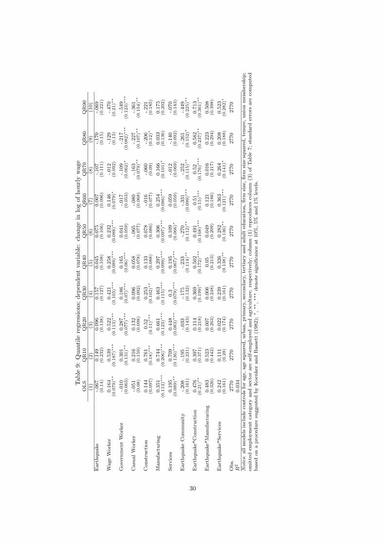
Tab

le9:

Qu

anti

lere

gre

ssio

ns;

dep

end

ent

vari

ab

le:

chan

ge

inlo

gof

hou

rly

wage

OL

SQ

R10

QR

20

QR

30

QR

40

QR

50

QR

60

QR

70

QR

80

QR

90

(1)

(2)

(3)

(4)

(5)

(6)

(7)

(8)

(9)

(10)

Eart

hqu

ake

-.067

0.1

49

0.0

96

0.1

57

0.0

45

0.0

75

0.0

07

-.107

-.170

-.069

(0.14)

(0.232)

(0.138)

(0.127)

(0.108)

(0.106)

(0.096)

(0.111)

(0.15)

(0.221)

Wage

Work

er0.1

64

0.5

39

0.5

22

0.4

21

0.2

58

0.2

32

0.1

46

-.012

-.129

-.470

(0.079)∗

∗(0

.187)∗

∗∗

(0.113)∗

∗∗

(0.103)∗

∗∗

(0.089)∗

∗∗

(0.088)∗

∗∗

(0.079)∗

(0.092)

(0.13)

(0.21)∗

∗

Gover

nm

ent

Work

er-.

010

0.3

01

0.2

87

0.1

86

0.1

65

0.0

41

-.017

-.109

-.217

-.549

(0.063)

(0.131)∗

∗(0

.077)∗

∗∗

(0.07)∗

∗∗

(0.06)∗

∗∗

(0.059)

(0.053)

(0.062)∗

(0.082)∗

∗∗

(0.123)∗

∗∗

Casu

al

Work

er-.

051

0.2

16

0.1

32

0.0

96

0.0

58

-.065

-.080

-.163

-.227

-.361

(0.08)

(0.159)

(0.098)

(0.092)

(0.078)

(0.077)

(0.068)

(0.079)∗

∗(0

.107)∗

∗(0

.154)∗

∗

Con

stru

ctio

n0.1

44

0.7

61

0.5

20.2

53

0.1

33

0.0

78

-.016

-.060

-.206

-.221

(0.097)

(0.18)∗

∗∗

(0.11)∗

∗∗

(0.102)∗

∗(0

.088)

(0.086)

(0.077)

(0.09)

(0.12)∗

(0.185)

Manu

fact

uri

ng

0.3

51

0.7

44

0.6

61

0.4

63

0.2

97

0.3

06

0.2

54

0.1

66

0.0

33

0.1

75

(0.113)∗

∗∗

(0.206)∗

∗∗

(0.123)∗

∗∗

(0.115)∗

∗∗

(0.099)∗

∗∗

(0.097)∗

∗∗

(0.086)∗

∗∗

(0.101)∗

(0.136)

(0.202)

Ser

vic

es0.1

95

0.7

09

0.4

48

0.3

0.1

95

0.1

09

0.0

59

-.012

-.140

-.070

(0.089)∗

∗(0

.136)∗

∗∗

(0.083)∗

∗∗

(0.079)∗

∗∗

(0.067)∗

∗∗

(0.066)∗

(0.059)

(0.069)

(0.092)

(0.143)

Eart

hqu

ake

Com

mu

nit

y-.

208

-.195

-.033

-.175

-.233

-.270

-.331

-.252

-.261

-.449

(0.161)

(0.231)

(0.143)

(0.132)

(0.114)∗

∗(0

.112)∗

∗(0

.099)∗

∗∗

(0.115)∗

∗(0

.152)∗

(0.225)∗

∗

Eart

hqu

ake*

Con

stru

ctio

n0.4

76

0.3

97

0.1

14

0.3

69

0.5

02

0.4

91

0.5

10.5

20.5

82

0.7

13

(0.21)∗

∗(0

.371)

(0.218)

(0.199)∗

(0.172)∗

∗∗

(0.168)∗

∗∗

(0.15)∗

∗∗

(0.176)∗

∗∗

(0.237)∗

∗(0

.361)∗

∗

Eart

hqu

ake*

Manu

fact

uri

ng

0.4

83

0.5

23

0.0

07

0.0

06

0.0

50.0

49

0.1

21

0.0

16

0.2

23

0.5

08

(0.326)

(0.442)

(0.263)

(0.248)

(0.213)

(0.209)

(0.186)

(0.217)

(0.294)

(0.398)

Eart

hqu

ake*

Ser

vic

es0.2

42

0.1

11

0.0

22

0.2

39

0.3

26

0.2

82

0.3

63

0.2

64

0.2

08

0.5

23

(0.161)

(0.28)

(0.174)

(0.161)

(0.138)∗

∗(0

.136)∗

∗(0

.121)∗

∗∗

(0.141)∗

(0.188)

(0.282)∗

Ob

s.2770

2770

2770

2770

2770

2770

2770

2770

2770

2770

R2

0.0

34

Notes:

all

mod

els

incl

ud

eco

ntr

ols

for

age,

age

squ

are

d,

urb

an

,p

rim

ary

,se

con

dary

,te

rtia

ryan

dad

ult

edu

cati

on

,fi

rmsi

ze,

firm

size

squ

are

d,

tenu

re,

un

ion

mem

ber

ship

;om

itte

dem

plo

ym

ent

cate

gory

an

dse

ctor

are

self

-em

plo

yed

an

dagri

cult

ure

,re

spec

tivel

y;

colu

mn

(1)

rep

rod

uce

sco

lum

n(3

)of

Tab

le7;

stan

dard

erro

rsare

com

pu

ted

base

don

ap

roce

du

resu

gges

ted

by

Koen

ker

an

dB

ass

ett

(1982);

∗,∗∗

,∗∗

∗d

enote

sign

ifica

nce

at

10%

,5%

an

d1%

level

s.

30

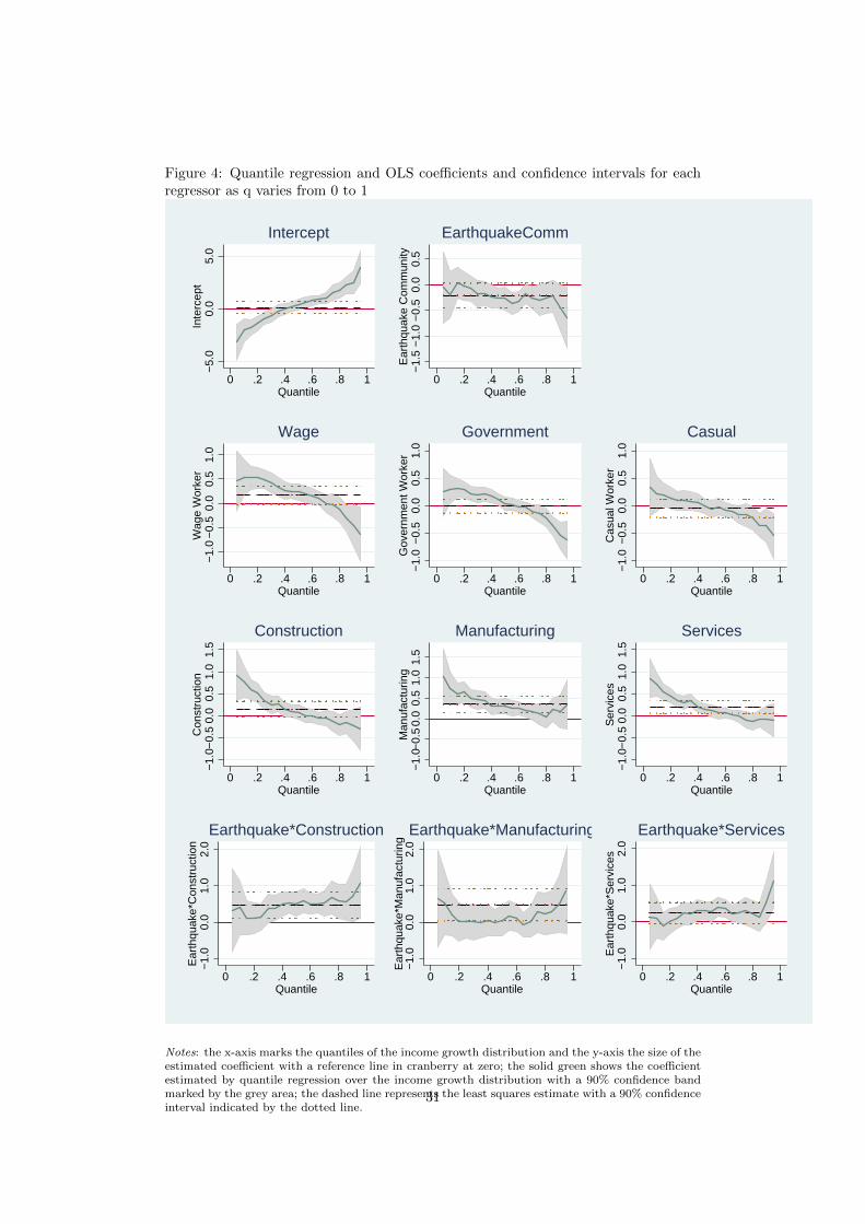
Figure 4: Quantile regression and OLS coefficients and confidence intervals for eachregressor as q varies from 0 to 1

−5.

00.

05.

0In

terc

ept

0 .2 .4 .6 .8 1Quantile

Intercept

−1.

5−

1.0

−0.

50.

00.

5E

arth

quak

e C

omm

unity

0 .2 .4 .6 .8 1Quantile

EarthquakeComm

−1.

0−

0.5

0.0

0.5

1.0

Wag

e W

orke

r

0 .2 .4 .6 .8 1Quantile

Wage−

1.0

−0.

50.

00.

51.

0G

over

nmen

t Wor

ker

0 .2 .4 .6 .8 1Quantile

Government

−1.

0−

0.5

0.0

0.5

1.0

Cas

ual W

orke

r

0 .2 .4 .6 .8 1Quantile

Casual

−1.

0−0.

50.

00.

51.

01.

5C

onst

ruct

ion

0 .2 .4 .6 .8 1Quantile

Construction

−0.

50.

00.

51.

01.

5−

1.0

Man

ufac

turin

g

0 .2 .4 .6 .8 1Quantile

Manufacturing−

0.5

0.0

0.5

1.0

1.5

−1.

0S

ervi

ces

0 .2 .4 .6 .8 1Quantile

Services

−1.

00.

01.

02.

0E

arth

quak

e*C

onst

ruct

ion

0 .2 .4 .6 .8 1Quantile

Earthquake*Construction

−1.

00.

01.

02.

0E

arth

quak

e*M

anuf

actu

ring

0 .2 .4 .6 .8 1Quantile

Earthquake*Manufacturing

−1.

00.

01.

02.

0E

arth

quak

e*S

ervi

ces

0 .2 .4 .6 .8 1Quantile

Earthquake*Services

Notes: the x-axis marks the quantiles of the income growth distribution and the y-axis the size of theestimated coefficient with a reference line in cranberry at zero; the solid green shows the coefficientestimated by quantile regression over the income growth distribution with a 90% confidence bandmarked by the grey area; the dashed line represents the least squares estimate with a 90% confidenceinterval indicated by the dotted line.

31