natural circulation characteristics at low-pressure...

Hindawi Publishing CorporationScience and Technology of Nuclear InstallationsVolume 2008, Article ID 874969, 14 pagesdoi:10.1155/2008/874969

Project ReportNatural Circulation Characteristics at Low-Pressure Conditionsthrough PANDA Experiments and ATHLET Simulations

Domenico Paladino,1 Max Huggenberger,1 and Frank Schafer2

1 Laboratory for Thermal-Hydraulics, Paul Scherrer Institute (PSI), 5232 Villigen, Switzerland2 Research Center Dresden-Rossendorf, P.O. Box 510119, 01314 Dresden, Saxony, Germany

Correspondence should be addressed to Frank Schafer, [email protected]

Received 31 July 2007; Accepted 2 January 2008

Recommended by John Cleveland

Natural circulation characteristics at low pressure/low power have been studied by performing experimental investigations andnumerical simulations. The PANDA large-scale facility was used to provide valuable, high quality data on natural circulationcharacteristics as a function of several parameters and for a wide range of operating conditions. The new experimental data allowfor testing and improving the capabilities of the thermal-hydraulic computer codes to be used for treating natural circulation loopsin a range with increased attention. This paper presents a synthesis of a part of the results obtained within the EU-Project NACUSP“natural circulation and stability performance of boiling water reactors.” It does so by using the experimental results produced inPANDA and by showing some examples of numerical simulations performed with the thermal-hydraulic code ATHLET.

Copyright © 2008 Domenico Paladino et al. This is an open access article distributed under the Creative Commons AttributionLicense, which permits unrestricted use, distribution, and reproduction in any medium, provided the original work is properlycited.

1. INTRODUCTION

In the framework of the EU-Project NACUSP, experimentson thermo-hydraulic characteristics of natural-circulation-cooled boiling water reactors (BWR) have been performedin four sophisticated thermo-hydraulic test facilities whichcomplement each other, ranging from small-scale to large-scale, and from low-pressure/low-power operating condi-tions to the nominal operating conditions for BWRs. Theultimate goal of the project was to improve the economics ofoperating and future plants through improved operationalflexibility, enhanced availability, and increased confidencelevels on the safety margins regarding the stability issues inBWRs [1].

This paper presents a synthesis of the results obtainedfrom the experiments performed in the large-scale PANDAfacility [2] and from the numerical simulations performedwith the thermal-hydraulic code ATHLET. The range ofparameters covers a large spectrum of conditions for thelow-pressure/low-power range, therefore, being of interestespecially with regard to the start-up procedures for natural-circulation-cooled BWRs (e.g., for the European simplifiedboiling water reactor (ESBWR)).

2. PANDA EXPERIMENTAL INVESTIGATIONS

2.1. PANDA facility

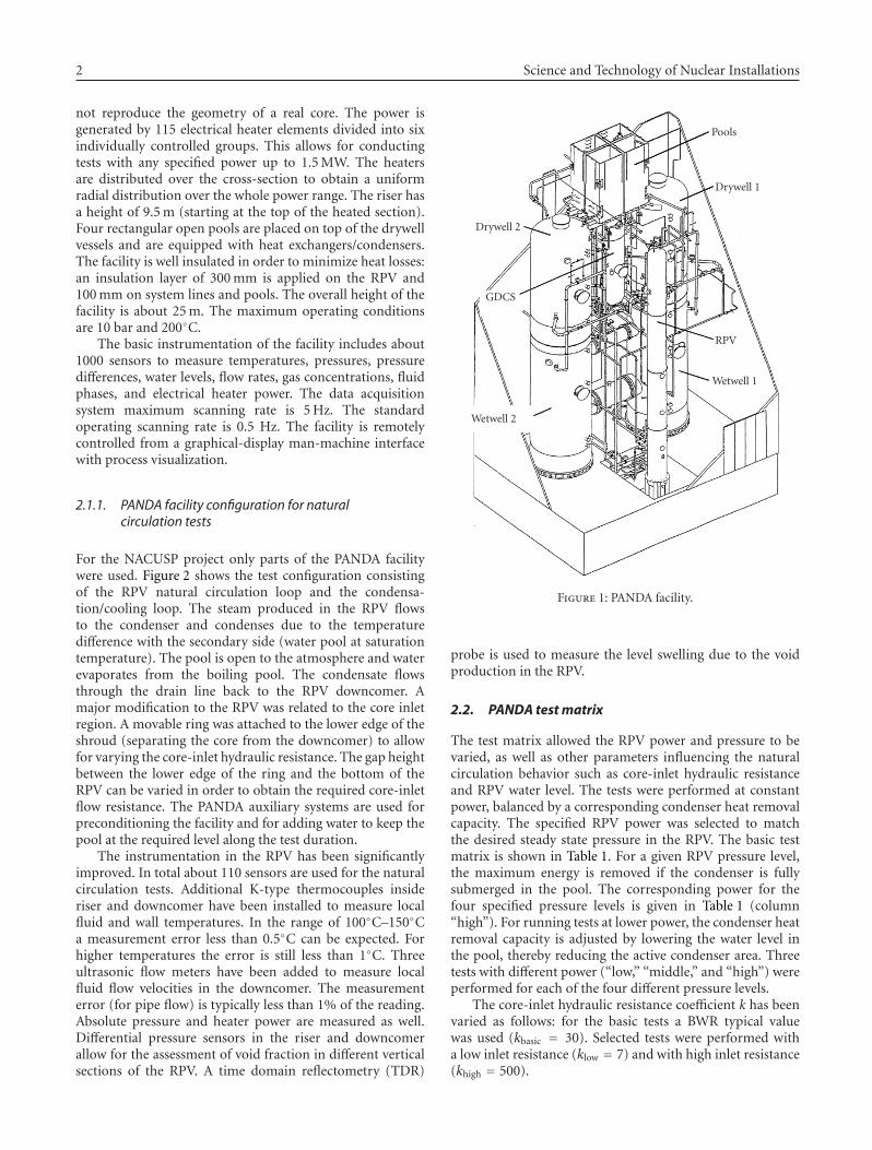
The multipurpose thermal-hydraulic test facility PANDA islocated at Paul Scherrer Institute (PSI), Villigen, Switzer-land. The facility is designed and used for investigating atlarge-scale system behavior and phenomena for differentlight water reactor (LWR) designs. PANDA has a modularstructure, which is based on six cylindrical pressure vesselswith a total volume of 460 m3 and four open pools witha total capacity of 60 m3 (Figure 1). Four of these pressurevessels are arranged in two vertical columns. The two lowervessels simulating the wetwell or suppression chamber areinterconnected with two large pipes. The wetwell vesselssupport the two vessels, simulating the drywell. They areinterconnected at about midplane elevation with one largepipe. The fifth vessel simulates the core flooding (GDCS)pool. The sixth vessel is configured to simulate the reactorpressure vessel (RPV). Its dimension allows for performingnatural circulation tests at roughly 1 : 1 scale in height. Thevessel has an inner diameter of 1.23 m and is 19.2 m in height.The RPV includes a heated section, a riser, and a downcomer(DC). The heated section has a height of 1.3 m and does

mailto:[email protected]

2 Science and Technology of Nuclear Installations

not reproduce the geometry of a real core. The power isgenerated by 115 electrical heater elements divided into sixindividually controlled groups. This allows for conductingtests with any specified power up to 1.5 MW. The heatersare distributed over the cross-section to obtain a uniformradial distribution over the whole power range. The riser hasa height of 9.5 m (starting at the top of the heated section).Four rectangular open pools are placed on top of the drywellvessels and are equipped with heat exchangers/condensers.The facility is well insulated in order to minimize heat losses:an insulation layer of 300 mm is applied on the RPV and100 mm on system lines and pools. The overall height of thefacility is about 25 m. The maximum operating conditionsare 10 bar and 200◦C.

The basic instrumentation of the facility includes about1000 sensors to measure temperatures, pressures, pressuredifferences, water levels, flow rates, gas concentrations, fluidphases, and electrical heater power. The data acquisitionsystem maximum scanning rate is 5 Hz. The standardoperating scanning rate is 0.5 Hz. The facility is remotelycontrolled from a graphical-display man-machine interfacewith process visualization.

2.1.1. PANDA facility configuration for naturalcirculation tests

For the NACUSP project only parts of the PANDA facilitywere used. Figure 2 shows the test configuration consistingof the RPV natural circulation loop and the condensa-tion/cooling loop. The steam produced in the RPV flowsto the condenser and condenses due to the temperaturedifference with the secondary side (water pool at saturationtemperature). The pool is open to the atmosphere and waterevaporates from the boiling pool. The condensate flowsthrough the drain line back to the RPV downcomer. Amajor modification to the RPV was related to the core inletregion. A movable ring was attached to the lower edge of theshroud (separating the core from the downcomer) to allowfor varying the core-inlet hydraulic resistance. The gap heightbetween the lower edge of the ring and the bottom of theRPV can be varied in order to obtain the required core-inletflow resistance. The PANDA auxiliary systems are used forpreconditioning the facility and for adding water to keep thepool at the required level along the test duration.

The instrumentation in the RPV has been significantlyimproved. In total about 110 sensors are used for the naturalcirculation tests. Additional K-type thermocouples insideriser and downcomer have been installed to measure localfluid and wall temperatures. In the range of 100◦C–150◦Ca measurement error less than 0.5◦C can be expected. Forhigher temperatures the error is still less than 1◦C. Threeultrasonic flow meters have been added to measure localfluid flow velocities in the downcomer. The measurementerror (for pipe flow) is typically less than 1% of the reading.Absolute pressure and heater power are measured as well.Differential pressure sensors in the riser and downcomerallow for the assessment of void fraction in different verticalsections of the RPV. A time domain reflectometry (TDR)

Pools

Drywell 1

RPV

Wetwell 1

Wetwell 2

GDCS

Drywell 2

Figure 1: PANDA facility.

probe is used to measure the level swelling due to the voidproduction in the RPV.

2.2. PANDA test matrix

The test matrix allowed the RPV power and pressure to bevaried, as well as other parameters influencing the naturalcirculation behavior such as core-inlet hydraulic resistanceand RPV water level. The tests were performed at constantpower, balanced by a corresponding condenser heat removalcapacity. The specified RPV power was selected to matchthe desired steady state pressure in the RPV. The basic testmatrix is shown in Table 1. For a given RPV pressure level,the maximum energy is removed if the condenser is fullysubmerged in the pool. The corresponding power for thefour specified pressure levels is given in Table 1 (column“high”). For running tests at lower power, the condenser heatremoval capacity is adjusted by lowering the water level inthe pool, thereby reducing the active condenser area. Threetests with different power (“low,” “middle,” and “high”) wereperformed for each of the four different pressure levels.

The core-inlet hydraulic resistance coefficient k has beenvaried as follows: for the basic tests a BWR typical valuewas used (kbasic = 30). Selected tests were performed witha low inlet resistance (klow = 7) and with high inlet resistance(khigh = 500).

Domenico Paladino et al. 3

Pool

Condenser

RPV

Water level nominal

Low (L L)

Low (L)

10500(Riser top)

6576

Drainline

Controlvalve

14443

Feedline

Riser

Down-comer

Electricalheaters

Adjustablecore inletflow resistance

Fm

Fm

Fm Fm (ultrasonic)

1000 (heater top, riser inlet)

0 (building floor)

−500 (RPV inside)

FM: Flow meter

RPV dimensions:

Height 19.2 mDiameter ID 1.23 mVolume 22.9 m3

Riser height 9.5 mRiser ID 1.05 m

Maximum operatingconditions:Power 1500 kWPressure 10 barTemperature 180 ◦C

Figure 2: PANDA configuration for natural circulation tests.

115 120 125 130 135

Temperature (◦C)

Test H2-1: RPV fluid temperatures

0

2

4

6

8

10

12

14

16

18

Hei

ght

(m)

Class 1

Water levelFlashing Top of the riser

Saturation temperature

Heated section

(a) Test H2.1

160 162 164 166 168 170 172 174 176 178 180

Temperature (◦C)

Test H8-1: RPV fluid temperatures

0

2

4

6

8

10

12

14

16

18

Hei

ght

(m)

Class 3

Water level

Boiling/flashing

Top of the riser

Saturation temperature

Heated section

(b) Test H8.1

Figure 3: Measured temperature profiles in the vertical axis of the RPV.


2000 2100 2200 2300 2400 2500 2600

Time (s)

Test L8.3: RPV flowmeters (over a 10 min period)

0

0.1

0.2

0.3

0.4

0.5

0.6

0.7

0.8

0.9

1

Vel

ocit

y(m

/s)

MVE.DC1

MVE.DC2

MVE.DC3

(a) Measured flow velocities in the downcomer

10−3 10−2 10−1 100

Frequency (Hz)

10−5

10−4

10−3

10−2

10−1

100

101

AP

SD(−

)

MVE.DC1MVE.DC2MVE.DC3

(b) Normalized power spectra of velocity signal

0 50 100 150 200 250 300 350 400

τ (s)

−1

−0.8

−0.6

−0.4

−0.2

0

0.2

0.4

0.8

0.6

1

AC

F(−

)

DR= A2/A1

A1A2

(c) ACF processed from one velocity signal

Figure 4: Analysis of flow velocity signals in the downcomer (Test L8.3).

Table 1: Basic test matrix (variation of pressure and power).

RPV pressure [bar]RPV power [kW]

Low Middle High

2.0 135 200 245

3.0 250 380 480

5.0 430 660 885

8.0 594 917 1306

The RPV water level has also been varied: most ofthe tests were performed with the collapsed water level at12.8 m above bottom of RPV. This level represents about thenominal value for the ESBWR. For few tests the water level

was reduced close to top of riser which is at 11.0 m aboveRPV bottom. The selected values were 11.1 m and 11.4 m.

The following three series of tests with totally 25experiments have been performed:

(i) B-series tests (BWR-typical core-inlet flow resistancek = 30):

(a) 12 tests with nominal RPV water level (12.8 m),

(b) 2 tests with low RPV water level (11.1 m and11.4 m);

(ii) L-series tests (Low core-inlet flow resistance k = 7):

(a) 3 tests with nominal RPV water level (12.8 m),

(b) 1 test with low RPV water level (11.1 m);


2000 2100 2200 2300 2400 2500 2600

Time (s)

Test B3.3: RPV flowmeters (over a 10 min period)

Vel

ocit

y(m

/s)

MVE.DC1

MVE.DC2

MVE.DC3

0

0.1

0.2

0.3

0.4

0.5

0.6

0.7

0.8

0.9

1

(a) Measured flow velocities in the downcomer

10−3 10−2 10−1 100

Frequency (Hz)

10−5

10−4

10−3

10−2

10−1

100

101

AP

SD(−

)

MVE.DC1MVE.DC2MVE.DC3

(b) Normalized power spectra of velocity signal

0 50 100 150 200 250 300 350 400

τ (s)

−1

−0.8

−0.6

−0.4

−0.2

0

0.2

0.4

0.8

0.6

1

AC

F(−

)

(c) ACF processed from one velocity signal

Figure 5: Analysis of flow velocity signals in the downcomer (Test B3.3).

(iii) H-series tests (High core-inlet flow resistance k=500):

(a) 6 tests with nominal RPV water level (12.8 m),(b) 1 test with low RPV water level (11.1 m).

An overview of all PANDA tests is included in Table 2.

2.3. Experimental results and analysis

Natural circulation modes

The coolant temperature increases in the heated section(core), but it may not reach saturation conditions under thegiven conditions. A rough estimation of the position of theboiling boundary in the core by means of a heat balancewas performed. The temperature measured at the inlet of the

core was used as the reference temperature, and the coarsestassumptions were made (no heat losses, uniform radial andvertical distribution of power in the core, no subcooledboiling). The nondimensional value z∗boil.b reported in Table 2corresponds to the distance (measured from the inlet of thecore, and divided by the length of the core) at which thisboiling boundary can be expected (z∗boil.b ≤ 1: boiling in thecore; z∗boil.b > 1: no boiling in the core). The result is thatboiling in the core did not occur in any test except may be intests with high core-inlet resistance and relatively high powerfor which z∗boil.b

∼= 1 is found.In the same way, a coarse estimation of the height in

the riser at which flashing may be expected to occur hasbeen made. Using the same inlet temperature, calculatingthe temperature at the outlet of the core, and assuming it is


Ta

ble

2:O

verv

iew

ofth

ePA

ND

Ate

sts

and

anal

ysis

resu

lts.

Test

nam

ek

PPo

wer

Leve

lRP

VLe

velp

oolT

subz∗ bo

il.bz∗ fl

ash

V1

V2

V3

V12

3V

ar12

3112

3f

TA

pD

RA

nal

ysis

ofR

PV

Cla

ss(b

ar)

(kW

)(m

)(m

)(K

)(–

)(–

)(m

/s)

(m/s

)(m

/s)

(m/s

)(m

2/s

2)

(%)

(Hz)

(sec

.)(d

eg)

(–)

pres

sure

sign

al

LOW

kSE

RIE

S:

L8.3

77.

9613

1312

.81

4.21

5.8

2.7

0.75

0.54

0.51

0.52

0.52

0.01

3522

0.01

6063

00.

641

maj

orp

eak,f=

0.01

455

(T=

65s)

;DR=

0.63

2

L5.3

75.

0490

912

.82

4.20

7.7

3.2

0.79

0.32

0.31

0.32

0.32

0.00

3017

0.00

8412

00

0.68

1m

ajor

pea

k,f=

0.00

84(T=

120

s);D

R=

0.68

2

LL5.

37

5.02

911

11.1

14.

205.

32.

60.

430.

350.

430.

370.

380.

0037

160.

0111

900

0.74

1m

ajor

pea

k,f=

0.01

1(T=

90s)

;DR=

0.74

2

L2.3

72.

0224

712

.83

4.20

13.8

12.5

1.02

0.16

0.20

0.21

0.19

0.00

3029

??

??

no

maj

orp

eak

1

BA

SIC

kSE

RIE

S:

B8.

130

8.04

594

12.7

51.

735.

83.

00.

820.

290.

23/

0.26

0.00

2720

??

??

1m

ajor

pea

k,f=

0.00

77(T=

130

s);D

R=

0.5?

1

B8.

230

8.06

917

12.8

12.

175.

82.

70.

770.

360.

310.

410.

360.

0052

200.

0115

870

0.6

1m

ajor

pea

k,f=

0.01

15(T=

87s)

;DR=

0.4?

2

B8.

330

7.98

1306

12.8

04.

205.

82.

70.

750.

520.

470.

570.

520.

0085

180.

0158

630

0.61

1m

ajor

pea

k,f=

0.01

58(T=

63s)

;DR=

0.4?

2

B5.

130

5.15

391

12.8

21.

737.

54.

00.

860.

190.

180.

180.

180.

0015

21?

??

?n

om

ajor

pea

k1

B5.

230

5.04

637

12.8

42.

177.

63.

10.

770.

220.

220.

230.

220.

0017

18?

??

?1

maj

orp

eak,f=

0.00

65(T=

154

s);D

R=

0.85

1

65.3

304.

8589

612

.77

4.20

7.8

2.8

0.72

0.30

0.27

0.26

0.28

0.00

3722

0.00

8012

50

0.66

1m

ajor

pea

k,f=

0.08

(T=

125

s);D

R=

0.65

2

BL-

5.3

305.

0289

611

.11

4.20

7.0

3.3

0.70

0.37

0.33

0.39

0.36

0.00

5520

??

??

1m

ajor

pea

k,f=

0.01

225

(T=

82s)

;DR=

0.4

1

BLL

5.3

304.

9589

711

.39

4.20

7.2

3.2

0.71

0.35

0.32

0.36

0.34

0.00

8527

0.01

0695

00.

851

maj

orp

eak,f=

0.01

055

(T=

95s)

;DR=

0.81

2

B3.

130

3.02

231

12.8

21.

7310

.48.

00.

960.

150.

160.

140.

150.

0026

34?

??

?n

om

ajor

pea

k1

B3.

230

3.02

361

12.8

02.

1710

.55.

80.

910.

180.

170.

160.

170.

0018

25?

??

?1

pea

k,f=

0.00

55(T=

182

s);

1

63.3

302.

9750

212

.78

4.21

10.7

4.7

0.87

0.20

0.18

0.19

0.19

0.00

1621

??

??

1p

eak,f=

0.05

5(T=

200

s);

1

B2.

130

2.02

111

12.8

11.

7314

.017

.91.

050.

100.

130.

120.

120.

0017

35?

??

?n

om

ajor

pea

k1

B2.

230

2.02

183

12.8

02.

1713

.812

.51.

010.

130.

150.

130.

140.

0024

35?

??

?n

om

ajor

pea

k1

B2.

330

2.00

241

12.8

04.

2013

.910

.20.

990.

140.

160.

160.

150.

0029

35?

??

?n

om

ajor

pea

k1

HIG

Hk

SER

IES:

H8.

150

07.

959

512

.81

1.73

5.2

1.4

0.25

/0.

130.

160.

140.

0023

34?

??

?n

om

ajor

pea

k3

H8.

350

07.

8313

0912

.78

4.21

4.6

1.2

0.03

/0.

260.

310.

29?

??

??

?n

om

ajor

pea

k3

H5.

150

05.

0641

912

.83

1.73

7.1

1.8

0.41

0.08

0.08

0.10

0.09

0.00

1444

??

??

no

maj

orp

eak

3

H5.

350

04.

9790

212

.81

4.20

6.6

1.3

0.12

0.15

0.12

0.17

0.15

0.00

3440

??

??

no

maj

orp

eak

3

HL5

.350

05.

0090

711

.10

4.21

6.0

1.5

0.23

0.22

0.16

0.23

0.20

0.01

7064

??

??

no

maj

orp

eak

3

H2.

150

02.

0313

112

.85

1.73

13.6

7.4

0.95

0.08

0.05

0.05

0.06

0.00

0641

??

??

no

maj

orp

eak

1

H2.

350

02.

0024

612

.83

4.20

13.6

4.6

0.84

0.08

0.06

0.07

0.07

0.00

8012

6?

??

?n

om

ajor

pea

k1


0 50 100 150

Transit time (s)

0

50

100

150

200

250

Osc

illat

ion

per

iod

(s)

L-series tests (low k)B-series tests (basic k)

Slope 1.6

Figure 6: Period of oscillation versus fluid transit time in core andriser.

conserved all along the riser (no heat losses), a distance z∗flash(measured from inlet of riser, and divided by length of riser)is estimated and reported in Table 2. For most of the tests,it is expected that flashing should only occur in the upperregion or above the riser. Of course, in tests at high core-inletresistance and relatively high power, and also in tests with lowRPV water level (and hence lower pressure head), this basiccalculation predicts flashing in lower sections of the riser.

These estimations do not take into account the 3Dand local effects that might affect the physical phenomenaand the flow regime actually occurring in the RPV. Someinteresting information can be retrieved by plotting someof the temperature profiles measured in the central axis ofthe RPV. Two examples are given in Figure 3, for which, acurve corresponding to the saturation temperature is alsoplotted on each graph. The saturation temperature hasbeen estimated by using the time-averaged RPV pressureand calculating the pressure head at each height, withoutconsidering the possible presence of void.

From Figure 3, it is clear that the validity of thecomparison with the saturation temperature may be limiteddue to the error in temperature measurements. Due tothe data reduction procedure, this error slightly increaseswith temperature (Figure 3). The saturation temperaturedecreases along the vertical axis as the system operates at lowpressure. Flashing should occur when the coolant reachessaturation conditions in the riser. Following this approach,in test H2.1 (shown in Figure 3(a)), the average height ofthe flashing boundary can be roughly estimated to be atabout the level corresponding to the top of the riser. Inthis case, flashing should be responsible for the shape ofthe profile above this height, where measured temperaturesseem to lie in the vicinity of the saturation curve. Thisbasically confirms the previous coarse prediction (Table 2,z∗flash = 0.95). In test H8.1, a different situation is shown(Figure 3(b)): the fluid temperature clearly following thesaturation curve indicates that two-phase flow should haveoccurred along the complete riser length. To summarize,

these different plots help to qualitatively distinguish differentcases and define three classes:

Class 1. flashing above the riser, or perhaps no flashing at all(Figure 3(a));

Class 2. flashing at a lower elevation in the riser;

Class 3. two-phase flow all along the riser (Figure 3(b)).Rough estimations of time-averaged void fraction valuesprocessed from differential pressure measurements alsoindicate that the highest void fraction was assessed at thetop of the riser, and especially for cases with high core-inlet resistance/high power (Class 3). These cases showedthe largest difference between the swell level (measured bythe TDR probe) and the collapsed water level retrieved fromdifferential pressure measurements. For example, in testsHL5.3 and H8.3, a void fraction of the order of 10% wasestimated in the upper region of the riser. In the lowersections, values lower than a few percent were found.

Analysis of flow velocity measurementsin RPV downcomer

The natural circulation flow rate is of main interest. Hence,this short analysis concerns the velocity measurements from3 ultrasonic flow meters in the RPV DC. The sensors arelocated at elevation 5.00 m above RPV bottom with an angleof 120◦ azimuthally between each other.

The velocity signals were sampled at a frequency of0.5 Hz for the whole duration of the test (5 hours). Itshould be noted that the time constant of the sensorswas set to 6 seconds in order to avoid aliasing problems.The autopower spectral density (APSD) of the signals wascalculated to identify resonance frequencies of the system.The autocorrelation function (ACF) was used to calculatethe decay ratio (DR) of the system. The DR is a widely usedparameter to quantify the stability of the system: if DR < 1,the system is linearly stable; if DR > 1, it is unstable. Inpractice, the DR values presented in Table 2 were estimatedby simply calculating the ratio between the second and thefirst maxima of the ACF (Figure 4(c)). Cross-power spectraldensities, coherence, and cross-correlation functions werealso calculated to examine coherence, possible phase shifts,and so forth between signals from different flow meters.

An overview of the results of the analysis performed canbe found in Table 2. The basic parameters of each test aregiven in the first columns of this table. Mean values of thevelocities calculated over the test period (V1, V2, and V3) arealso reported. V123 is the average of the three mean velocities.The quantity I123 should provide an estimate of the intensityof the velocity fluctuations, and was calculated as follows:

I123(%) = 100.

(Var123

)1/2

V123, (1)

where Var123 represents the average of the 3 variances of thesignals. It should be realized that this relation could result invery high values for the tests with very low natural circulation


Table 3: Initial conditions for the selected PANDA tests (Exp. = Experiment, Cal. = ATHLET Calculation, Add. Calc. = Additional ATHLETcalculation).

Test

Power MW.RP.7 RPV pressure RPV level DC velocity DC temperature

(kW) MP.RP.1 (bar) ML.RP.1 (m) MVE.DC.1 (m/s) MTL.RP.1 (◦C)

Exp. Cal. Exp. Cal. Exp. Cal. Exp. Cal. Exp. Cal.

B3.3 502 502 2.97 2.98 12.78 12.78 0.19 0.19 133.7 133.4

B5.2 637 637 5.04 5.06 12.84 12.85 0.22 0.22 152.1 152.3

L5.3 909 909 5.04 5.05 12.82 12.83 0.32 0.32 152.0 152.3

LL5.3 911 911 5.02 5.02 11.11 11.23 0.38 0.38 151.5 152.1

B8.3 1306 1306 7.98 7.99 12.80 12.86 0.52 0.52 169.7 170.5

Add. Calc. — 1308 — 4.9 — 11.43 — 0.60 — 151.2

Table 4: Oscillation period and decay ratio calculated from the DCmass flow (Exp. = experiment, Cal. = ATHLET calculation).

TestPeriod (s) Decay ratio (–)

Exp. Cal. Exp. Cal.

B3.3 200.0 204.8 — 0.66

B5.2 154.0 170.7 — 0.61

L5.3 120.0 113.8 0.68 0.62

LL5.3 90.0 102.4 0.74 0.55

B8.3 63.0 68.3 0.61 0.60

velocities, for which the signal-to-noise ratio is expected tobe higher (e.g., test H2.3).

Concerning the spectral analysis, the frequency and thecorresponding period of the major peak are reported whenpossible. The value “0” in the column “Δϕ” of Table 2means that no significant phase shift between the signals wasobserved, that is, the three velocity signals were oscillatingin phase at one given frequency. When possible, a DR wasestimated from the ACF and is also reported in Table 2. Onecolumn of the table refers to the analysis of signals fromthe sensor measuring the total pressure in the RPV. Theseadditional observations may help to characterize some ofthe tests. Looking at the spectra and at the results of thisanalysis based on the ACF and the estimation of DR values,the PANDA tests can be categorized in two different groupsas follows.

1st group

The rows in Table 2 corresponding to these tests are greyed.An illustration of this case is made using test L8.3 results. Anexcerpt of the raw velocity signals recorded during this test isshown in Figure 4(a). A major peak can be observed on theprocessed spectra of the 3 sensors reported in Figure 4(b).The time traces of the velocity signals show that the threesensors oscillate “together,” that is, with no significant phaseshift between each other. This was confirmed by lookingat the phase of the complex cross-power spectral densitiesbetween the different signals. Just simply looking at a numberof raw signals recorded over the test period, it can also be seenthat the other measured variables (temperatures, pressurein the RPV, condenser feed, and drain flows, etc.) show

fluctuations with the same frequency. The ACF obtainedfrom velocity signal 1 is given in Figure 4(c). Clearly, aDR value indicating stable behavior (DR = 0.64) can beestimated from this graph.

2nd group

An illustration of this group is given using test B3.3 results.Observations made on the raw signals (Figure 5(a)) in thiscase show rather random behavior. In some other testsbelonging to the same group, it is sometimes possibleto observe significant phase shifts between the sensors.Figure 5(b) shows that there is no longer a major peakpresent in the power spectrum. Using a logarithmic scale,the low-frequency part of the spectrum appears to be flatter.Moreover, the ACF does not really allow a DR value to bederived (Figure 5(c)), this DR appearing to be much smaller(actually, very close to 0) compared to the tests of the firstgroup.

It was also observed that these two characteristic modesof behavior, indicated by the ACF plots, did not vary as afunction of time during the course of the tests. For tests L8.3and B3.3, this was done by calculating ACFs over 5 successive(1-hour long) time periods and it clearly showed that, in bothcases, all the ACFs for one test at different times were verysimilar.

Some data from other sensors (condenser feed and drainflow rates, RPV pressure, etc.) have also been analyzed usingthe same approach as for the velocity data. For the testsfrom the 1st group, a resonance peak can be observed atthe same oscillation frequency. No peak can be found forthe tests belonging to the 2nd group. However, in some ofthese tests (e.g., test B3.3), the condenser feed flow and RPVpressure signals may exhibit a peak in their spectrum whereasno such peak was observed for the velocity signals (see alsothe second last column of Table 2, concerning the analysis ofRPV pressure signals). This indicates that flashing possiblytakes place above the top of the riser, not influencing themain circulation flow. These cases fall consistently into Class1 (see Figure 3).

From the expected mechanism of the flow oscillations,the fluid travelling time in the heated section, and thetransit time of the enthalpy perturbations in the adiabaticsection, should play a role in determining the period of the


oscillations. From Figure 11, it is clear that the oscillationperiod decreases with increasing average flow rate. The totaltransit time can be evaluated as the sum of the transit timein the riser section plus half of the transit time in the heatedsection [3]. In PANDA, no velocity measurement is availablein the riser. An estimation of the riser velocity was made bysimply using the time-averaged value of the velocity in theDC reported in Table 2, and just considering the flow arearatio between the riser and the DC.

Following this simplified approach, the oscillation periodwas found to be in the order of 1.6 times the transit timeof the fluid (Figure 6). The simple way in which the transittime was estimated did not consider the occurrence of two-phase flow in the riser. Hence, it is likely that our assessmentoverestimated this time. Thus, these observations seem to bequite consistent with those presented for the CIRCUS facility[1], for which the period of oscillation was found to be twicethe transit time.

Discussion

The differentiation between the two groups of tests is basedon DR values derived from the velocity signals. However, thevalidity and the accuracy of this method can be questioned.Many other methods have been used to extract stabilityparameters and can be compared to the ACF-based method.For this reason, some of our experimental velocity timetraces were processed using a more sophisticated method,namely, the autoregressive method. This method properlyapplied to our signals yielded about the same DR values asthose presented in Table 2. This confirms the main resultfrom this analysis that all tests are stable.

However, by having a closer look to the tests, the differentflow regimes that can be assumed, and the three classesdefined, can be related to the previous findings regarding thestability of the system. Information reported in Table 2 wasused for this purpose. The plots in Figure 3 partly illustratethe following classification.

Class 4 (Figure 3(a)). High inlet subcooling and relativelylow (or even very low) flow rates characterize this class. It islikely that flashing occurred only above the riser, the naturalcirculation flow still being in a single-phase regime. Thiswould explain why, in some of these tests, contrary to thevelocity signals in the DC, some RPV pressure signals showa peak in their spectrum and allow the derivation of DRvalues (see, e.g., test B5.2). It is also possible that in some ofthese tests (notably those performed at the lowest powers),no flashing occurred at all in the whole system.

Class 5. These tests, performed at relatively high powerand low inlet resistance, have been characterized by a well-identified oscillation period and DR values could be derivedfrom the velocity signals. The highest natural circulationflow rates were measured in these tests, which indicatethe combined effect of the flow enhancement by steamproduction and of a low inlet resistance. According to ourestimations and analyses, no boiling occurred in the core butflashing did in the upper half of the riser.

Class 6 (Figure 3(b)). Very stable behavior was found forthese tests performed with an increased inlet resistance.Under these conditions, the flashing front fluctuates closeto the bottom of the riser, which stabilizes very much thetwo-phase natural circulation. The measured flow rates areamong the lowest of the test series, as a result of the high flowresistance. Looking at the parameters (notably the expectedposition of the boiling boundary) reported in Table 2 andat the characteristic temperature profiles (Figure 3(b)), itseems that stable two-phase natural circulation flow can beassumed in these cases.

The presented classification gives a rather coherentpicture of the PANDA test series. It was possible to link theexperimental observations with the expected phenomenol-ogy. No unstable tests were recorded. However, the charac-terization of the tests (from single-phase to two-phase flowconditions) is satisfying and quite consistent with what isreported in the literature. Test BLL5.3, which shows a DR ofabout 0.85, should be very close to unstable conditions.

The test matrix allowed the variation of the RPV waterlevel. However, the actual influence of this parameter on theflow behavior cannot be clearly assessed. Comparing testsB5.3 and BL5.3, it seems that a lower level would have astabilizing effect.

3. ATHLET SIMULATIONS

3.1. Thermal-hydraulic model

The thermal-hydraulic code ATHLET [4], which has beendeveloped by GRS (Gesellschaft fur Anlagen- und Reaktor-sicherheit mbH), was used for the calculation of selectedexperiments from the PANDA test matrix (see Section 2).The ATHLET input dataset models all main parts ofthe PANDA configuration used for the NACUSP naturalcirculation experiments (Figure 7).

The ATHLET model consists of the lower plenum (P1-LP-1), the core section (P1-CORE) with 115 electrical heaterelements, the riser (P1-RIS1), upper plenum (P1-UP-1),downcomer (P1-DC), and the upper part of the RPV(P1-RIS2). The isolation condenser (IC) is not modeled.Therefore, a bypass (CIRC-ENT, CIRC-EIN) is connected tothe upper part of the RPV and to the downcomer, modelingthe IC-feed and drain lines by fills with constant mass flowsand given enthalpy (only drain line). In all control volumes,the 5-equation model (separate conservation equations forliquid and vapour mass and energy, mixture momentumequation) and the full-range drift-flux model of ATHLET areused. A valve at the lower end of the downcomer (VLV, seeFigure 7) is used to model different k-factors of the core inlet.The cross-section of this valve can be changed to adjust thecore inlet flow resistance.

3.2. Steady state calculation

At first, a steady state calculation with constant boundaryconditions was performed for each PANDA test. With helpof these calculations, the pressure losses, heat losses, the RPV


z = 19.2 m

z = 11 m

z = 1.5 m

z = 0 m

P1-RIS2

P1-RIS1

P1-UP-1

P1-CORE VLV

P1-LP-1 H-P1-CORE

P1-DC

CIRC-EIN

CIRC-ENT

Figure 7: Schematic representation (a) and ATHLET model (b) of PANDA test facility.

water level, and the temperature distribution were adjusted.The steady state calculation starts with zero power. After afew seconds, the core power is switched on and the power isincreased with time. For the calculations, it was not possibleto specify a certain k-factor for the core inlet, becausethe form-loss coefficients are changed within the algorithmof the ATHLET code during the steady state calculation.Therefore, a valve at the lower end of the downcomer withchanging cross-section was used to adjust the core-inlet flowresistance. The cross-section of this valve was reduced toa value, which leads to DC velocities corresponding to themeasured data. The steady state calculation is stopped ifstable conditions are reached. As an example, the resultsof the steady state calculation for Test B 8.3 and thecorresponding experimental data are shown in Figure 8.

3.3. Transient calculations

From the PANDA test matrix, 5 experiments were selectedfor the ATHLET simulations. Table 3 shows the initial

conditions calculated with ATHLET in comparison to themeasured data. For the experiments the data were recordedover a period of 5 hours. The experimental data in Table 3represent average values. The initial conditions for theATHLET simulations correspond to the end of the steadystate calculations.

Each transient calculation starts from a steady statecalculation as described in Section 3.2. To simulate thesystem behavior with respect to natural circulation stabilitya short disturbance of the drain line mass flow was used inorder to stimulate oscillations in the loop (see Figure 9). Theresponse of the system can be seen in the calculated riser massflow.

As in the experiments, the DC velocities were used tocalculate the spectrum and the decay ratio. Figure 10 showsthe downcomer velocity, the spectrum, and the autocorre-lation function for two ATHLET calculations (Test B 8.3and Test B 3.3). Both calculations predict stable behaviorand no limit-cycle oscillations occur. The disturbance of thedrain line mass flow leads to flow oscillations with decreasing


−1000 −800 −600 −400 −200 0

Time (s)

10

11

12

13

14×102

Pow

er(k

W)

MW.RP.7 - experimentMW.RP.7 - ATHLET

(a)

−1000 −800 −600 −400 −200 0

Time (s)

6

7

8

9

Pre

ssu

re(b

ar)

MP.RP.1 - experimentMP.RP.1 - ATHLET

(b)

−1000 −800 −600 −400 −200 0

Time (s)

8

10

12

14

Leve

l(m

)

ML.RP.1 - experimentML.RP.1 - ATHLET

(c)

−1000 −800 −600 −400 −200 0

Time (s)

0

0.5

1

1.5

Vel

ocit

y(m

/s)

MVE.DC.1 - experimentMVE.DC.1 - ATHLET

Test B8.3

(d)

Figure 8: Core power (MW.RP.7), system pressure (MP.RP.1), RPV level (ML.RP.1), and downcomer velocity (MVE.DC.1) for test B 8.3:experiment and ATHLET steady state calculation.

0 100 200 300 400 500 600

Time (s)

−2

−1

0

1

2

Mas

sfl

ow(k

g/s)

CIRC-EIN - ATHLETCIRC-ENT - ATHLET

(a)

0 100 200 300 400 500 600

Time (s)

0

100

200

300

400

Mas

sfl

ow(k

g/s)

P1-RIS1 - ATHLET

Test B 8.3

(b)

Figure 9: Mass flow in IC-feed and drain lines (CIRC-EIN, CIRC-ENT) and riser mass flow (P1-RIS1).


0 500 1000 1500

Time (s)

0

0.5

1

DC

velo

city

(m/s

)

ATHLET - test B 8.3ATHLET - test B 3.3

(a)

0 0.02 0.04 0.06 0.08 0.1

Frequency (Hz)

0

0.02

0.04

0.06

Spec

tru

m


(b)

0 100 200 300 400 500

Time (s)

−1

−0.5

0

0.5

1

Au

toco

rrel

atio

nfu

nct

ion


PANDA test B 8.3Experiment ATHLET

DC velocityOscillation periodDecay ratio

0.52 m/s63 s0.61

0.52 m/s68.3 s0.6

PANDA test B 3.3Experiment ATHLET

DC velocityOscillation periodDecay ratio

0.19 m/s200 s

-

0.19 m/s204.8 s0.66

(c)

Figure 10: DC velocity, spectrum, and autocorrelation function for the ATHLET calculations of tests B 8.3 and B 3.3.

amplitude. In both cases, the oscillations were damped dueto the higher core-inlet loss coefficient (k = 30) used in theB-series experiments. Although the oscillations were dampedin the ATHLET simulations, an oscillation period and also adecay ratio can be calculated from the DC mass flow. Table 4gives a comparison between measured and calculated periodand decay ratio for the selected PANDA tests.

The experiments and also the ATHLET calculations showthat the oscillation period decreases with increasing DC

velocity. This behavior is illustrated in Figure 11. The resultsof the ATHLET calculations show a good agreement with theexperimental data.

To demonstrate the ability of ATHLET to calculate anunstable behavior with the PANDA model, an additionalcalculation with a core-inlet loss coefficient of k = 7, ahigher core power, and a lower RPV level was performed.The initial conditions for this calculation are given in Table 3.The results of the simulation show an unstable behavior with


0.1 0.2 0.3 0.4 0.5 0.6 0.7

DC velocity (m/s)

0

50

100

150

200

250

Osc

illat

ion

per

iod

(s)

Experiment L seriesExperiment B seriesATHLET calculation

ATHLET test B 3.3

ATHLET test B 5.2

ATHLET test L 5.3ATHLET test LL 5.3

ATHLET test B 8.3ATHLETadditionalcalculation

Figure 11: Oscillation period as a function of the DC velocity forthe PANDA tests and the ATHLET simulations.

strong oscillations caused by flashing in the riser section.Figure 12 shows the calculated DC mass flow, the spectrum,and the autocorrelation function. The oscillations have aperiod of 62 seconds with a decay ratio >0.9.

In Figure 13, the calculated temperature distributionover the height of the PANDA model is illustrated for t =5000 seconds. At this time, the dynamic behavior becomesunstable. The subcooling in the core is high and no voidproduction takes place. Only above the middle of the risersection, the temperature reaches saturation conditions andflashing-induced oscillations occur.

4. CONCLUSIONS

In the PANDA facility, 25 tests have been carried out in orderto investigate natural circulation flow behavior and stability,under low-pressure/low-power conditions. Some parametersinfluencing the natural circulation flow were varied, suchas the RPV power and pressure, the core-inlet hydraulicresistance, and also the water level in the RPV.

An analysis of the data from three ultrasonic sensorsinstalled at three circumferential locations in the downcomerwas presented. The power spectra show, in a few tests, amajor and unique resonance peak. The period of oscillationof the flow rate seems to be of the order of twice the transittime of the fluid in the riser. Analyses of the time seriesshow that these cases are stable. The tests for which moreflat spectra were obtained show a behavior that is even morestable.

A phenomenological classification has been appliedaccording to three circulation modes that could be assumed:single-phase circulation (with possibly flashing above theriser), two-phase circulation with flashing in the upper halfof the riser, or two-phase flow along the complete riserlength. The new experimental data about the behavior ofthe natural circulation flow under low-pressure conditionsrepresent a valuable extension of the available database,

5400 5600 5800 6000 6200 6400

Time (s)

0

1

2

DC

velo

city

(m/s

)

(a)

0 0.02 0.04 0.06 0.08 0.1

Frequency(Hz)

0

0.1

0.2

0.3

Spec

tru

m

(b)

0 100 200 300 400 500

Time (s)

−1

−0.5

0

0.5

1

Au

toco

rrel

atio

nfu

nct

ion

ATHLET additional calculationPower 1308 kWRPV pressure 4.9 barRPV level 11.43 m

DC velocity 0.6 m/sOscillation period 61 sDecay ratio > 0.9

(c)

Figure 12: DC velocity, spectrum, and autocorrelation functionfor the additional ATHLET calculation with higher core power andlower RPV level.


145 150 155 160

↑ ↓

↑↑

Temperature (◦C)

0

5

10

15

20

Hei

ght

(m)

Saturation temperatureFluid temperature

LP core

Ris

erU

pper

plen

um

t = 5000 s

Figure 13: Temperature distribution over the height of the PANDAmodel (additional ATHLET calculation).

notably because the height of the riser in PANDA is approx-imately preserved with respect to a real reactor. The datahave been used for assessing the capabilities and limitationsof thermal-hydraulics codes in predicting natural circulationcharacteristics at low pressure/low power.

The ATHLET simulations show stable behavior for theselected PANDA tests. In all simulations, the oscillations weredamped and no limit-cycle oscillations occur. The calculatedperiods and decay ratios show a good agreement with theexperimental results. With help of the additional calculation,it could be demonstrated that ATHLET can also simulatean unstable behavior. In this case, strong oscillations occur,caused by flashing in the riser section.

ACKNOWLEDGMENT

This work was supported by the European Commission (EU5th Framework Program on Nuclear Fission Safety, NACUSPProject) and by the Swiss Federal Office for Education andScience.

REFERENCES

[1] C. Aguirre, D. Caruge, F. Castrillo, et al., “Natural circulationand stability performance of BWRs (NACUSP),” NuclearEngineering and Design , vol. 235, no. 2–4, pp. 401–409, 2005.

[2] O. Auban, D. Paladino, and R. Zboray, “Experimental investiga-tion of natural-circulation flow behavior under low-power/low-pressure conditions in the large-scale PANDA facility,” NuclearTechnology , vol. 148, no. 3, pp. 294–312, 2004.

[3] A. Manera and T. H. J. J. van der Hagen, “Stability ofnatural-circulation-cooled boiling water reactors during start-up: experimental results,” Nuclear Technology , vol. 143, no. 1,pp. 77–88, 2003.

[4] G. Lerchl and H. Austregesilo, ATHLET Mod 1.2 Cycle B: User’sManual, Munich, Germany, August 1999.

TribologyAdvances in

Hindawi Publishing Corporationhttp://www.hindawi.com Volume 2014

International Journal of

AerospaceEngineeringHindawi Publishing Corporationhttp://www.hindawi.com Volume 2010

FuelsJournal of


Journal ofPetroleum Engineering


Industrial EngineeringJournal of


Power ElectronicsHindawi Publishing Corporationhttp://www.hindawi.com Volume 2014

Advances in

CombustionJournal of


Journal of


Renewable Energy

Submit your manuscripts athttp://www.hindawi.com


StructuresJournal of

International Journal of

RotatingMachinery


EnergyJournal of


Hindawi Publishing Corporation http://www.hindawi.com

Journal ofEngineeringVolume 2014

Hindawi Publishing Corporation http://www.hindawi.com Volume 2014

International Journal ofPhotoenergy


Nuclear InstallationsScience and Technology of


Solar EnergyJournal of


Wind EnergyJournal of


Nuclear EnergyInternational Journal of


High Energy PhysicsAdvances in

The Scientific World JournalHindawi Publishing Corporation http://www.hindawi.com Volume 2014

natural circulation characteristics at low-pressure...

Documents