narrow-band frequency modulation -...

Narrow-band Frequency Modulation

KEEE343 Communication Theory

Lecture #16, May 3, 2011Prof. Young-Chai [email protected]

Summary

·•Narrowband Frequency Modulation

·•Wideband Frequency Modulation

Narrow-Band Frequency Modulation

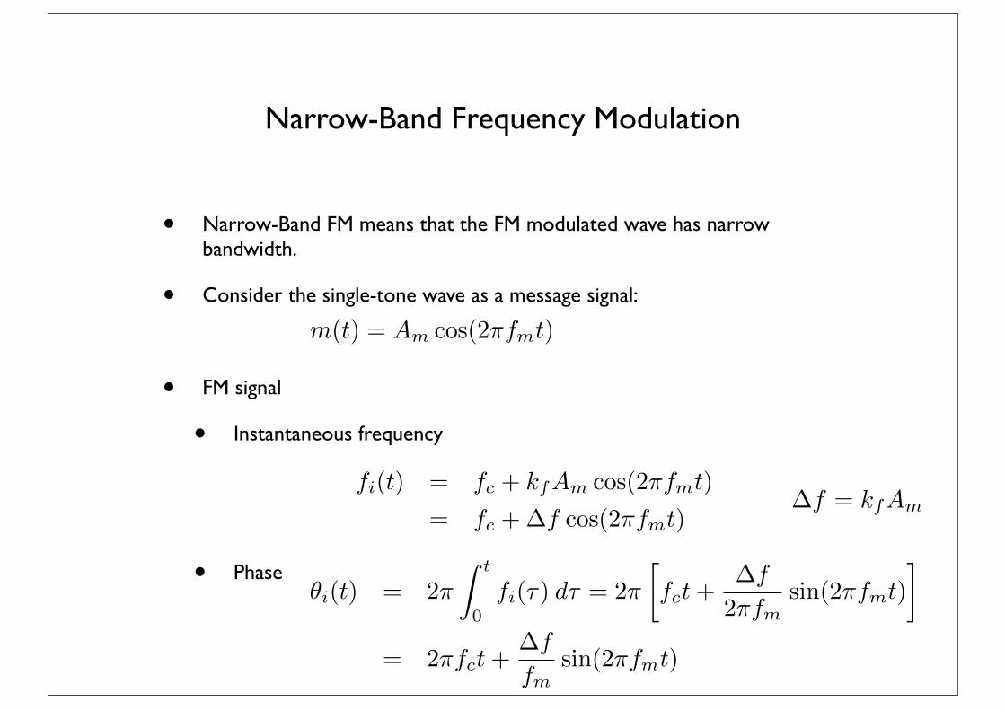
• Narrow-Band FM means that the FM modulated wave has narrow bandwidth.

• Consider the single-tone wave as a message signal:

• FM signal

• Instantaneous frequency

• Phase

m(t) = Am cos(2�fmt)

fi(t) = fc + kfAm cos(2�fmt)

= fc +�f cos(2�fmt)

�i(t) = 2⇥

Z t

0fi(⇤) d⇤ = 2⇥

fct+

�f

2⇥fmsin(2⇥fmt)

�

= 2⇥fct+�f

fmsin(2⇥fmt)

�f = kfAm

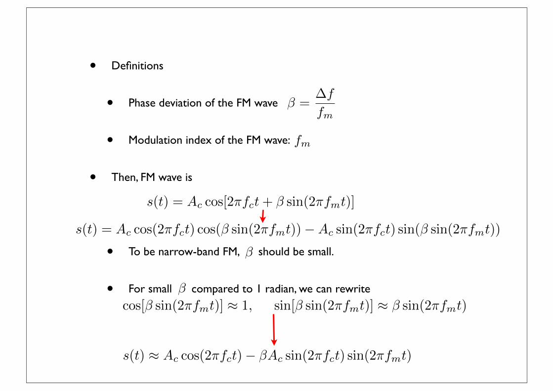
• Definitions

• Phase deviation of the FM wave

• Modulation index of the FM wave:

• Then, FM wave is

• To be narrow-band FM, should be small.

• For small compared to 1 radian, we can rewrite

� =�f

fm

s(t) = Ac cos[2⇥fct+ � sin(2⇥fmt)]

fm

s(t) ⇡ Ac cos(2⇥fct)� �Ac sin(2⇥fct) sin(2⇥fmt)

s(t) = Ac cos(2⇥fct) cos(� sin(2⇥fmt))�Ac sin(2⇥fct) sin(� sin(2⇥fmt))

�cos[� sin(2⇥fmt)] ⇡ 1, sin[� sin(2⇥fmt)] ⇡ � sin(2⇥fmt)

�

[Ref: Haykin & Moher, Textbook]

• Consider the modulated signal

which can be rewritten as

where

and

Polar Representation from Cartesian

s(t) = a(t) cos(2�fct+ ⇥(t))

s(t) = sI(t) cos(2�fct)� sQ(t) sin(2�fct)

sI(t) = a(t) cos(�(t)), and, sQ(t) = a(t) sin(�(t))

a(t) =⇥s2I(t) + s2Q(t)

⇤ 12 , and �(t) = tan�1

sQ(t)

sI(t)

�

• Approximated narrow-band FM signal can be written as

• Envelope

• Maximum value of the envelope

• Minimum value of the envelope

s(t) ⇡ Ac cos(2⇥fct)� �Ac sin(2⇥fct) sin(2⇥fmt)

for small�

a(t) = Ac

⇥1 + �2 sin2(2⇥fmt)

⇤⇡ Ac

✓1 +

1

2�2 sin2(2⇥fmt)

◆

Amax

= Ac

✓1 +

1

2�2

◆

Amin = Ac

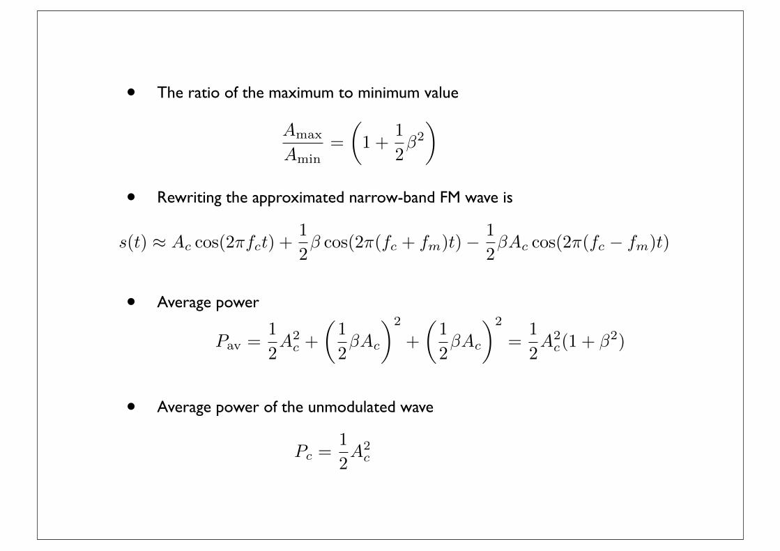
• The ratio of the maximum to minimum value

• Rewriting the approximated narrow-band FM wave is

• Average power

• Average power of the unmodulated wave

Amax

Amin

=

✓1 +

1

2�2

◆

s(t) ⇡ Ac cos(2⇥fct) +1

2

� cos(2⇥(fc + fm)t)� 1

2

�Ac cos(2⇥(fc � fm)t)

Pav =1

2A2

c +

✓1

2�Ac

◆2

+

✓1

2�Ac

◆2

=1

2A2

c(1 + �2)

Pc =1

2A2

c

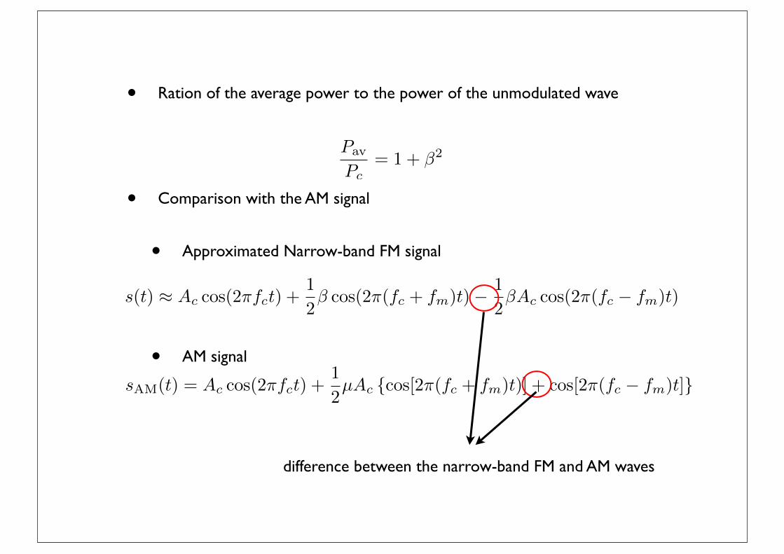
• Ration of the average power to the power of the unmodulated wave

• Comparison with the AM signal

• Approximated Narrow-band FM signal

• AM signal

Pav

Pc= 1 + �2

s(t) ⇡ Ac cos(2⇥fct) +1

2

� cos(2⇥(fc + fm)t)� 1

2

�Ac cos(2⇥(fc � fm)t)

sAM(t) = Ac cos(2�fct) +1

2

µAc {cos[2�(fc + fm)t)] + cos[2�(fc � fm)t]}

difference between the narrow-band FM and AM waves

• Bandwidth of the narrow-band FM:

• Phasor interpretation

2fm


• Angle

• Using the power series of the tangent function such as

⇥(t) = 2⇤fct+ ⌅(t) = 2⇤fct+ tan�1(� sin(2⇤fmt))

tan�1(x) ⇥ x� 1

3x

3 + · · ·

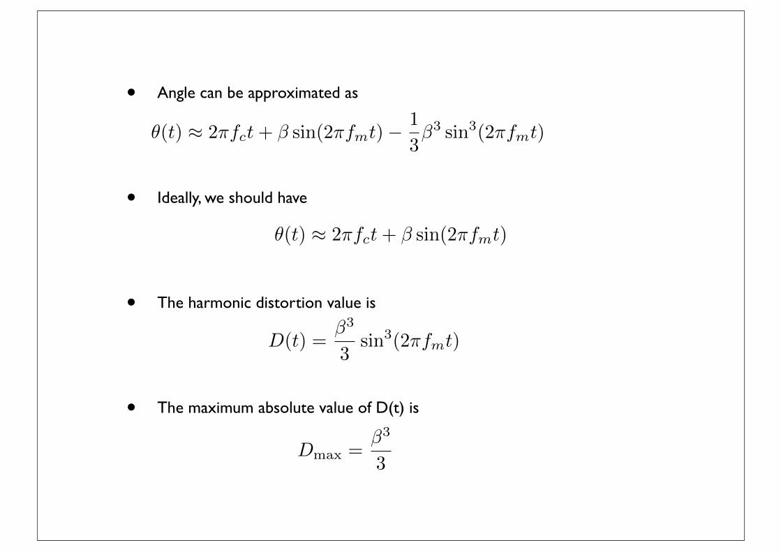
• Angle can be approximated as

• Ideally, we should have

• The harmonic distortion value is

• The maximum absolute value of D(t) is

⇥(t) ⇡ 2⇤fct+ � sin(2⇤fmt)

D(t) =�3

3sin3(2⇥fmt)

⇥(t) ⇡ 2⇤fct+ � sin(2⇤fmt)� 1

3�3 sin3(2⇤fmt)

Dmax

=�3

3

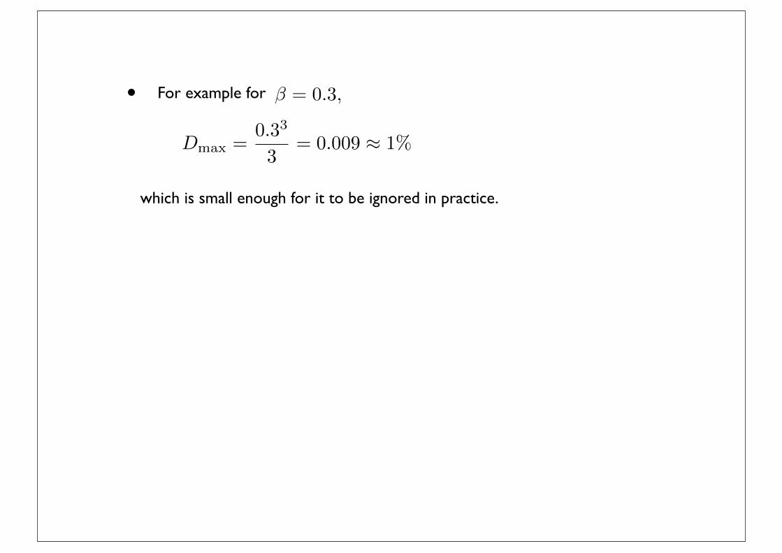
• For example for

which is small enough for it to be ignored in practice.

� = 0.3,

Dmax

=0.33

3= 0.009 ⇡ 1%

Amplitude Distortion of Narrow-band FM

• Ideally, FM wave has a constant envelope

• But, the modulated wave produced by the narrow-band FM differ from this ideal condition in two fundamental respects:

• The envelope contains a residual amplitude modulation that varies with time

• The angle contains harmonic distortion in the form of third- and higher order harmonics of the modulation frequency

�i(t)fm

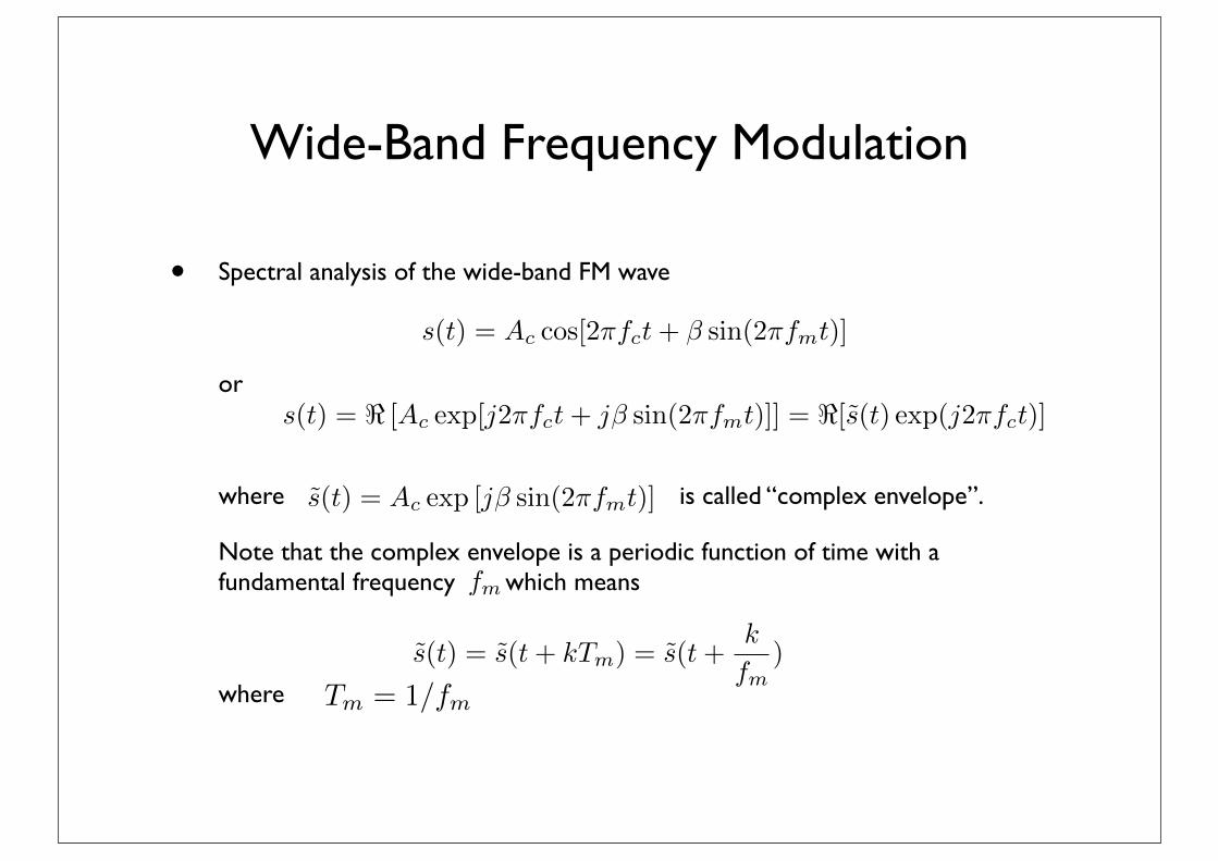
Wide-Band Frequency Modulation

• Spectral analysis of the wide-band FM wave

or

where is called “complex envelope”.

Note that the complex envelope is a periodic function of time with a fundamental frequency which means

where

s(t) = Ac cos[2⇥fct+ � sin(2⇥fmt)]

s(t) = < [Ac exp[j2⇥fct+ j� sin(2⇥fmt)]] = <[s̃(t) exp(j2⇥fct)]

s̃(t) = Ac exp [j� sin(2⇥fmt)]

fm

s̃(t) = s̃(t+ kTm) = s̃(t+k

fm)

Tm = 1/fm

• Then we can rewrite

• Fourier series form

where

s̃(t) =

1X

n=�1cn exp(j2�nfmt)

cn = fm

Z 1/(2fm)

�1/(2fm)s̃(t) exp(�j2⇥nfmt) dt

= fmAc

Z 1/(2fm)

�1/(2fm)exp[j� sin(2⇥fmt)� j2⇥nfmt] dt

s̃(t) = s̃(t+ k/fm)

= Ac exp[j� sin(2⇥fm(t+ k/fm))]

= Ac exp[j� sin(2⇥fmt+ 2k⇥)]

= Ac exp[j� sin(2⇥fmt)]

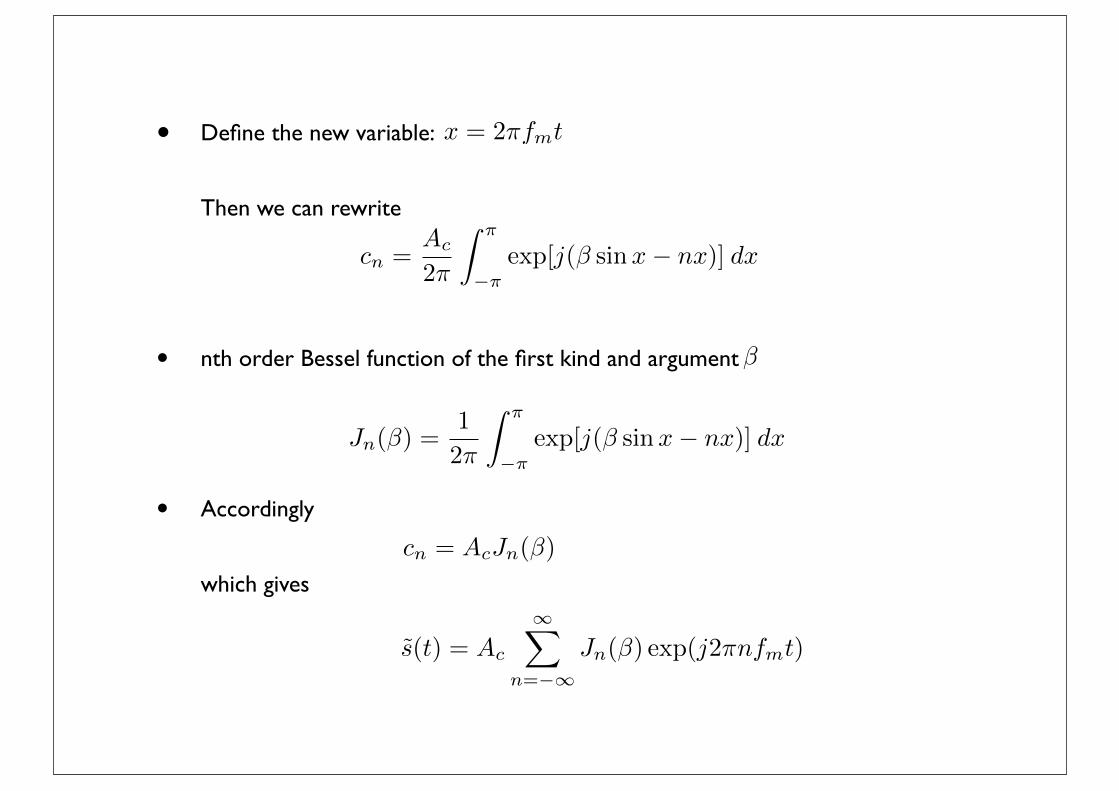
• Define the new variable:

Then we can rewrite

• nth order Bessel function of the first kind and argument

• Accordingly

which gives

x = 2�fmt

cn =

Ac

2⇥

Z �

��exp[j(� sinx� nx)] dx

�

Jn(�) =1

2⇥

Z �

��exp[j(� sinx� nx)] dx

cn = AcJn(�)

s̃(t) = Ac

1X

n=�1Jn(�) exp(j2⇥nfmt)

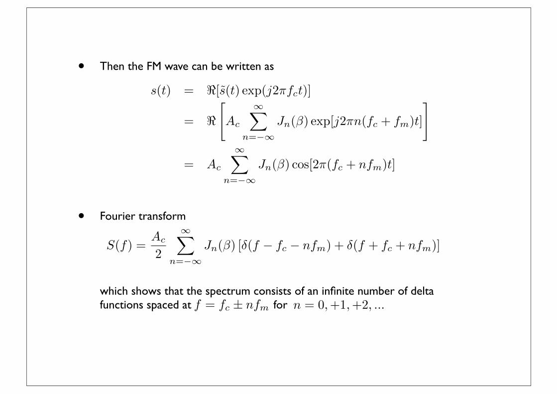
• Then the FM wave can be written as

• Fourier transform

which shows that the spectrum consists of an infinite number of delta functions spaced at for

s(t) = <[s̃(t) exp(j2⇥fct)]

= <"Ac

1X

n=�1Jn(�) exp[j2⇥n(fc + fm)t]

#

= Ac

1X

n=�1Jn(�) cos[2⇥(fc + nfm)t]

S(f) =Ac

2

1X

n=�1Jn(�) [⇥(f � fc � nfm) + ⇥(f + fc + nfm)]

f = fc ± nfm n = 0,+1,+2, ...

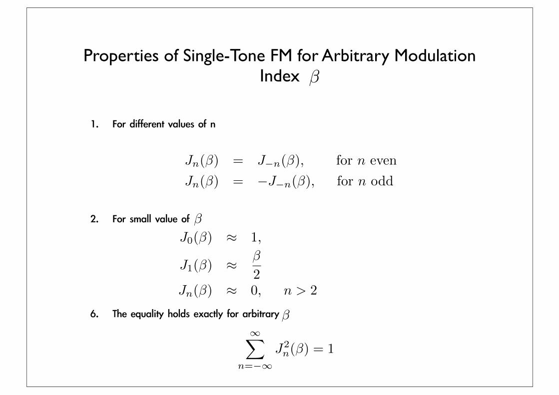
1. For different values of n

2. For small value of

6. The equality holds exactly for arbitrary

Properties of Single-Tone FM for Arbitrary Modulation Index �

Jn(�) = J�n(�), for n even

Jn(�) = �J�n(�), for n odd

J0(�) ⇡ 1,

J1(�) ⇡ �

2Jn(�) ⇡ 0, n > 2

�

�1X

n=�1J2n(�) = 1

1. The spectrum of an FM wave contains a carrier component and and an infinite set of side frequencies located symmetrically on either side of the carrier at frequency separations of ...

2. The FM wave is effectively composed of a carrier and a single pair of side-frequencies at .

3. The amplitude of the carrier component of an FM wave is dependent on the modulation index . The averate power of such as signal developed across a 1-ohm resistor is also constant:

The average power of an FM wave may also be determined from

fm, 2fm, 3fm

fc ± fm

�

Pav =1

2A2

c

Pav =1

2A2

c

1X

n=�1J2n(�)

narrow-band frequency modulation -...

Documents