narrative explanation of econometric demand equations for

1

Narrative Explanation of Econometric Demand Equations for Market Dominant Products Filed with Postal Regulatory Commission on January 20, 2021

Prepared for the Postal Regulatory Commission

Postal Regulatory CommissionSubmitted 7/1/2021 10:57:37 AMFiling ID: 119133Accepted 7/1/2021

1

Estimation of Econometric Demand Equations

A. Basic Demand Equation

The econometric demand equations filed with the Postal Regulatory Commission on

January 20, 2021 take the following form:

Vt = a∙x1te

1∙x2te

2∙…∙xnte

n∙εt (Equation 1)

where Vt is volume at time t, x1 to xn are explanatory variables, e1 to en are elasticities

associated with these variables, and εt represents the residual, or unexplained, factor(s)

affecting mail volume.

In general, variables which are believed to substantially influence the demand for

mail are introduced into an econometric equation as a quarterly time series in which the

elasticity of mail volume with respect to the particular variable is estimated using a

Generalized Least Squares estimation procedure. The explanatory variables

considered here include Postal prices, measures of macroeconomic activity (e.g.,

employment, investment), measures of mail trends (e.g., volume losses to electronic

and Internet diversion), seasonal variables, and other variables as warranted.

The functional form of Equation 1 is used by the Postal Service because it has been

found to model mail volume quite well historically, and because it possesses two

desirable properties. First, by taking logarithmic transformations of both sides of

Equation 1, the natural logarithm of Vt can be expressed as a linear function of the

natural logarithms of the Xi variables as follows:

ln(Vt) = ln(a) + e1•ln(x1t) + e2•ln(x2t) + e3•ln(x3t) +...+ en•ln(xnt) + ln(εt) (Equation 1L)

Equation 1L satisfies traditional least squares assumptions and is amenable to

solution by Ordinary Least Squares. Second, the ei parameters in Equation 1L are

2

exactly equal to the elasticities with respect to the various explanatory variables.

Hence, the estimated elasticities do not vary over time, nor do they vary with changes to

either the volume or any of the explanatory variables. Because of these properties, this

demand function is sometimes referred to as a constant-elasticity demand specification.

For explanatory variables which are logged in the equation, then, the coefficients

which come out of these demand equations can be interpreted directly as elasticities.

B. Explanatory Variables

1. Price

a. Own-Price Measures

The starting point for traditional micro-economic theory is a demand equation that

relates quantity demanded to price. Quantity demanded is inversely related to price.

That is, if the price of a good were increased, the volume consumed of that good would

be expected to decline, all other things being equal.

This fundamental relationship of price to quantity is modeled in the Postal Service’s

demand equations by including the price of postage in each of the demand equations

estimated by the Postal Service for mail categories and services which have a price

(i.e., excluding Postal Penalty mail and Free for the Blind and Handicapped Mail).

The Postal prices entered into these demand equations are calculated as weighted

averages of the various rates within each particular category of mail. For example, the

price of First-Class single-piece letters is a weighted average of the single-piece

stamped letters rate (55 cents), the single-piece metered letters rates (50 cents), the

additional ounce rate (15 cents), and the nonstandard surcharge (15 cents)1. Product-

by-product billing determinants provide the components of the market baskets which are

used as weights in developing these price measures. The price indices used in the

1 Rates as of January 27, 2019.

3

demand equations filed with the Commission on January 20, 2021, were constructed

using chain-weighted price indices.

Chain-weighted price indices compare each period with the proceeding one such

that the weight and price reference periods are moved forward each period. In this way,

chain-weighted price indices capture the substitution effect of price changes, as

consumers may shift consumption between categories in response to changes in

relative prices. In addition, chain-weighted price indices account for shifts in the mix of

consumer goods over time due to non-price related consumer preferences which

ultimately alters the effective average price of consumer goods. The periods referred to

in the first sentence of the paragraph refer to specific price regimes so that the price

indices do not change between quarters when Postal rates do not change.

The most recent set of weights used in constructing these prices were FY 2019

billing determinants.

Looking at the historical relationship between mail volumes and Postal prices

suggests that mailers may not react immediately to changes in Postal rates. For some

types of mail, it may take up to a year for the full effect of changes in Postal rates to

influence mail volumes. To account for the possibility of a lagged reaction to changes in

Postal prices on the demand for certain types of mail, the Postal price may be entered

into the demand equations lagged by up to four quarters. The exact number of lags

used is an empirical question which is answered on a case-by-case basis.

Prices are expressed in the Postal Service’s demand equations in real dollars. The

consumer price index (CPI-U) is used to deflate the prices.

In general, when the Postal Service refers to own-price elasticities, the reference is

to long-run own-price elasticities. The long-run own-price elasticity of a mail category is

equal to the sum of the coefficients on the current and lagged price of mail in the

relevant demand equation. The long-run own-price elasticity therefore reflects the

4

cumulative impact of price on mail volume after allowing time for all of the lag effects to

be felt.

b. Other Price Measures

The price of postage is not the only price paid by most mailers to send a good or

service through the mail. For those cases where the non-Postal price of mail is

significant and for which a reliable time series of non-Postal prices is available, these

prices may also be included explicitly in the demand equations used to explain mail

volume.

There is one example of such a price included in some of the equations presented

here, trade-weighted exchange rates, which are included as an explanatory variable in

most of the econometric demand equations associated with International Mail (both

inbound and outbound).

Changes in the value of the U.S. dollar vis-à-vis foreign currencies can make the

price of foreign goods more or less attractive relative to the price of similar domestic

goods, which may affect the volume of such goods delivered through the Postal

Service.

c. Postal Cross-Price Relationships

In the past, some of the Postal Service’s econometric demand equations have

included cross-price measures with other Postal products, such as First-Class Single-

Piece and Workshared Letters, and Bound Printed Matter and Media Mail. In some

cases, these cross-price variables entered the equations in the same way as the own-

price variables, i.e., as a measure of the average price of the product. In other cases,

however, cross-price variables were measured in relative terms (i.e., the difference

between the prices of two Postal products).

5

As has been the case for several years now, the econometric demand equations

filed with the Postal Regulatory Commission on January 20, 2021, do not include any

such cross-price variables. The exclusion of such variables was first discussed in some

detail in the response to the Chairman’s Information Request No. 8, question 5, which

was filed with the Commission on March 8, 2010. As explained in that response, the

decision of whether to include a particular cross-price relationship in a particular

econometric demand equation was made on a case-by-case basis. In all cases, the

overriding goal of all of the Postal Service’s econometric work is to produce the most

accurate volume forecasts possible. As a general rule, the most accurate volume

forecasts are obtained from econometric demand equations which best model the

historical demand for mail volume. So, while it ended up being the case that, in fact,

there were no cross-price or discount variables included in any of the econometric

demand equations filed on January 20, 2021, this was not the result of a general

decision to exclude all such variables from the Postal Service’s equation, but was,

instead, the result of a series of careful analyses of each of the Postal Service’s

individual demand equations.

This is not, however, to say that mailers may not at times shift from one mail

subclass to another in response to a change in Postal rates. In fact, however, such

changes tend to overwhelmingly be responses to specific and unusual changes in

relative rate structures associated with a specific rate change. Rather than attempting

to model such changes through a blunt one-size-fits-all instrument such as an

aggregate price index or an average discount level, the effect of such changes is,

instead, better modeled through the inclusion of either dummy variables or non-linear

intervention analysis. An example of a case-specific mailer shift between mail

subclasses is the impact of R2006-1 (May, 2007) on Marketing Mail Letters, when the

elimination of Automation Carrier-Route Letters rates led to a shift of volume from Basic

ECR to Marketing Mail Letters.

6

2. Impact of the Economy on Mail Volumes

In addition to being affected by prices, mail volumes are also affected by the state of

the economy. For example, as incomes rise, people are able to purchase more goods

and services, and this is generally true of the use of Postal services which tend to

perform better during periods of stronger economic growth and stagnate or decline

during periods of weaker economic growth (or decline). A stronger economy is also

likely to increase business use of the mail. To model these relationships, the demand

equations used by the Postal Service typically include one or more macroeconomic

variables which relate mail volumes to general economic conditions.

a. Macroeconomic Variables Used Here

Three key macroeconomic variables are used in the Postal Service’s econometric

market-dominant demand equations: private employment, gross private domestic

investment, and e-commerce retail sales. These data are compiled by the United

States government and, with the exception of e-commerce sales, are obtained by the

Postal Service from IHS Global Insight, an independent economic forecasting firm. At

various times, consumption expenditures, total retail sales, mail-order retail sales,

personal disposable income, gross domestic product (GDP), and the difference

between actual and potential GDP (the output gap) have also been explored as

candidate explanatory variables.

The specific variable choices are made on an equation-by-equation basis. The

decision process in choosing macroeconomic variables includes an effort to develop

equations which are both theoretically correct as well as empirically robust.

Dollar-denominated variables (e.g., business investment spending) are entered into

the equations in real terms. All economic variables are also entered on a per adult

7

basis, consistent with the structure of the mail volume demand equations which are

estimated on a per adult basis.

(i) Employment

Total private employment is included in several of the Postal Service’s econometric

demand equations, including First-Class and Periodicals Mail. In addition, the demand

equation for Alaska Bypass mail includes total non-farm employment in Alaska.

The theoretical rationale for including total employment as a macro-economic

variable is that in many cases, mail volume is not affected by the dollar value of

economic transactions, so much as by the number of such transactions. For example,

the number of credit card bill payments one makes does not necessarily go up as the

total amount charged per card goes up. While variables like GDP or retail sales may be

good measures of the total dollar amount of economic activity (e.g., the total amount

charged per credit card), employment appears to be a better measure of the number of

business transactions (e.g., number of bills paid).

Ultimately, the choice of which macroeconomic variable to use in a demand equation

is an empirical decision based on which variable best fits the volume data.

(ii) Investment

Advertising can be viewed as a type of business investment in that it represents

expenditures today for the purpose of generating revenues in the future. As such,

direct-mail advertising volume is likely to be affected by the same factors which drive

business investment spending. To reflect this relationship, real gross private domestic

investment is included as an explanatory variable in the demand equations for

Marketing Mail and Bound Printed Matter Flats filed with the Commission on January

20, 2021.

8

(iii) E-Commerce Sales

Parcel and package service volumes, such as Bound Printed Matter Parcels and

Media Mail volumes consist, in large part, of the delivery of products bought by the

sender or recipient of the mail. This type of mail volume derives primarily from retail

sales. More specifically, package delivery services are largely a function of online retail

sales which are subsequently delivered to the consumer. Hence, e-commerce retail

sales are included directly in the demand equations for most of the Postal Service’s

parcel and package service equations.

3. The Internet and Electronic Diversion

One of the most significant issues facing the Postal Service in recent decades has

been the threat, both realized and potential, of electronic diversion of mail. E-mail has

emerged as a potent substitute for personal letters and business correspondence. Bills

can be paid electronically, either as online payments or through an automatic deduction

from a bank account, and bills and statements can be received through the Internet

rather than through the mail. Virtually all magazines and newspapers now have an

online edition as a complement to their print editions, and in some cases, the print

edition has been eliminated in favor of an all-online format. Understanding the

emergence of the Internet and its role vis-à-vis the mail is critical in understanding mail

volume, both today and in the future.

There are two general dimensions to the Internet which are important to understand

in assessing the extent to which the Internet, and other electronic alternatives, may

serve as possible substitutes for mail volume: the breadth of Internet usage and the

depth of Internet usage.

9

i. Breadth of Internet Use

The breadth of Internet usage refers generally to the number of people online. As

more people use the Internet, there are simply more people for whom the Internet is

available as a substitute for the mail.

Increases in the breadth of Internet use can explain a large share of historical

electronic diversion. More recently, however, the breadth of Internet usage has not

increased significantly as Internet penetration has largely levelled off in the United

States.

ii. Depth of Internet Use

The depth of Internet usage refers to the number of things which an individual does

on the Internet. As the depth of Internet usage increases for a particular person, the

number of activities for which the Internet can substitute for mail may increase, thereby

increasing the overall level of substitution of the Internet for mail volume, even in the

absence of an increase in the number of Internet users.

The breadth and depth of Internet usage have both been important in understanding

the impact of the Internet on mail volumes historically. However, moving forward, the

depth of Internet usage is a much more important consideration. The reason for this is

that the breadth of Internet usage has a natural ceiling. Eventually, everybody who

would ever obtain Internet access will have Internet access. At that point, the only

source of increasing electronic diversion of the mail will be an increasing depth of

Internet usage. Hence, in measuring the impact of the Internet and other electronic

alternatives on mail volumes, it is important to measure the impact not only of the

breadth of Internet usage in the United States, but the depth of Internet (and other

electronic) usage as well.

10

iii. Use of Trends to Model Internet Diversion

Beginning in the early 2000s, the Postal Service introduced one or more explicit

measures of Internet usage in several of its demand equations as a means of capturing

the impact of the Internet (and other electronic delivery alternatives) on mail volumes.

These variables – which included consumption expenditures on Internet Service

Providers, the number of households with Broadband Internet access, and the number

of Global Internet Servers - reflected primarily the breadth of Internet use – i.e., the

number of people on the Internet. As noted above, however, the story of Internet

diversion of mail has more recently been a story of increasing depth of Internet use.

To better measure the increasing depth of Internet use, the Postal Service’s

methodology for modeling Internet and other electronic diversion has changed more

recently. For the market-dominant demand equations filed with the Commission on

January 21, 2020, diversion is not modeled via explicit Internet variables, but, instead, is

measured through a series of linear time trends which start at various times within the

sample periods over which the Postal Service’s demand equations are estimated.

The use of trends to measure Internet diversion was discussed at length in Thomas

Thress’s responses to Presiding Officer’s Information Requests (POIRs) in Docket No.

R2013-11. See, for example, Mr. Thress’s responses to POIR No. 3, question 1; POIR

No. 6, question 12; and POIR No. 9, question 7 in that case.

Diversion trends of this kind are estimated in many of the Postal Service’s demand

equations. Time trends of this type are special cases of Intervention Analysis. The

technical details of Intervention Analysis are described later in this document.

11

4. The Great Recession

The 2008-2009 recession, sometimes called the “Great Recession”, had a larger

negative impact on many categories of mail volume than can be explained by the

macroeconomic variables included in the Postal Service’s demand equations. In these

cases, the Postal Service models the unique impacts of the Great Recession on mail

volumes using Intervention Analysis techniques. The technical details of Intervention

Analysis are described next.

5. Intervention Analysis

In some cases, mail volumes may be affected by unique events, or “interventions”.

Oftentimes, the effect of such factors can be modeled via trend or dummy variables. In

other cases, however, the impact of such “interventions” on mail volumes may be more

complicated than can be fully captured by a set of linear variables. In such cases, a

more elaborate non-linear Intervention analysis is undertaken to more accurately model

the impact of some factors on some types of mail.

Two examples of Interventions for which this type of analysis is undertaken are the

two factors just discussed: Internet Diversion and the Great Recession.

a. Non-Linear Intervention

Intervention analysis is a time series technique which allows one to identify the

effects of an event over time. An “intervention” is an event which affects the demand for

a given product. There are essentially three different types of impact of intervention

events: step functions, pulse functions, and trends. A generalized Intervention Analysis

technique allows for a functional form which is flexible enough to accommodate all of

these possibilities as dictated by the underlying data. This function is called the transfer

function.

12

The role of the transfer function is to allow the input variable to affect the volume in

different ways and rates over time. Therefore, the impact of an intervention on volume is

the product of a particular transfer function and an input variable. The general form of

the transfer function is given by:

( )

( )

2 3

0 1 2 3

2 3

1 2 3 3

...

1 ...

iS T S Ti

t t tj

B B B B BI B B

B B B B B

− − − −= =

− − − − (Equation 2)

where B is the lag operator: S

t t SB y y −= . For the stability of the model, the roots of the

equations 2

0 1 2 .. 0i

iB B B − − − − = and 2

1 21 .. 0j

jB B B − − − − = must lie outside the unit

circle. Of course, a more generalized form of Equation 2 is necessary to limit the

number of ω and δ parameters so that the equation can be uniquely estimated.

The ω(B) terms represent the level impact of the intervention event. For example, in

Equation 2, if ωi=0, for i>0, then the intervention will only affect volume in the current

period, and Equation 2 will simplify to a dummy variable equal to one in the quarter of

interest and zero elsewhere with coefficient ω0. If, on the other hand, ωi = ωj, for all i,j,

with δi = 0 for all i, then Equation 2 simplifies to a dummy variable equal to one from the

quarter of interest forward with coefficient ω0 (=ωi for all i). Finally, if ωi is an increasing

(or decreasing) function of i, then the transfer equation identified above will simplify to a

trend response to the intervention event of interest.

The δ(B) terms represent the rate of increase or decrease of the intervention events,

e.g., the rate of change from a short-run to a long-run impact. For simplicity, δi is

typically assumed to be constant across all i. That is, the rate of adoption of an

intervention event is typically assumed to be constant over time.

A transfer function that allows for each of the three possibilities outlined above -

pulse, step, or trend response to an intervention – is shown in Equation 3 below:

13

It = {ω0 + ω1B / (1 – δB) + (ω2 + ω3t)B / (1 – B)}Pt (Equation 3)

where Pt is a pulse function – i.e., Pt = 1 for the period of the intervention, zero

elsewhere.

A step function (equal to 1 for the period of the intervention and all subsequent

periods), St, can be expressed as a function of Pt using lag notation so that St = Pt / (1-

B).

In Equation 3, ω0 is equal to the initial response to the Intervention event. If

ω1=ω2=ω3=0, then the response to the Intervention will be equal to zero in all

subsequent periods, and the transfer function will be a pure pulse function (Pt). If

ω0=ω1 and δ=ω2=ω3=0, then the transfer function will be a pure step function (St = Pt /

(1-B)). If ω1=ω2=0 and ω0= ω3, then the transfer function will be a pure linear trend. If,

on the other hand, none of these equalities are realized, then Equation 3 will explain a

more flexible transfer function as dictated by the observed data.

The functional form of Equation 3, which expresses the transfer function as a

function of the lag operators may not be intuitively obvious. Re-expressing the lag

operator notation here into more conventional notation yields Equation 4:

It = ω0·Pt + ω1·(Pt-1+δ1Pt-2+δ2Pt-3+…) + ω2·St + ω3·Tt·St (Equation 4)

where, as noted above, Pt is equal to one during the period of the intervention, zero

elsewhere (both before and after), St is equal to zero prior to the intervention event

being modeled, and equal to one thereafter, and T is a time trend equal to zero at the

point of the intervention event, increasing by one each quarter thereafter.

While Equation 4 is a function of only 5 parameters – δ and ωi for i = 0 to 3 – it

nonetheless technically requires the inclusion of an infinite number of terms in the

demand equation of interest. It turns out, however, that, at any given point in time, each

14

of the Pt-i terms is equal to zero except for, at most, one. To see this, one can re-write

Equation 4 as follows:

It = ω0·Pt + ω1·Σi=1∞(δi-1Pt-i) + ω2·St + ω3·Tt·St

When Tt = 1, the value of Pt-1 = 1, Pt-i = 0, for all i≠1. Similarly, when Tt = 2, the

value of Pt-2 = 1, Pt-i = 0, for all i≠2. So, instead of a sum over all values of Pt-i one can

instead replace i with Tt-1 in the above equation. That is,

It = ω0·Pt + ω1·St·(δTt-1) + ω2·St + ω3·Tt·St (Equation 5)

Intervention variables of the form in Equation 5 are then added to the Postal

Service’s econometric demand equations as necessary. The Intervention parameters -

ω0, ω1, ω2, ω3, and δ – are estimated simultaneous with the other econometric

parameters using non-linear least squares.

Intervention Analysis of this type is used to model unique aspects of the Great

Recession on several classes of mail, including First-Class Single-Piece Letters and

Flats, Commercial Marketing Letters, and Bound Printed Matter Parcels.

b. S-Curves

One common source of trends in data that are difficult to model econometrically by

relating behavior to other economic variables is the problem of market penetration.

Research into the rate at which new products or new technology are adopted has

shown that a typical adoption cycle for a new product is initially gradual, followed by

increasingly-rapid adoption until some point in time at which the adoption curve reaches

an inflection point and the rate of adoption slows until the adoption curve eventually

plateaus and the product or technology exhibits a more traditional stable growth pattern

15

attributable to common economic factors. An adoption curve of this sort can be

modeled through a type of logistic curve, commonly called an “s-curve” because its

shape approximates the letter “s”.

S-curves take the form:

St = z1∙dt / (1 + z2∙exp(-z3∙tt) ) + … (Equation 6)

where dt is a dummy variable equal to one starting in the initial period of the s-curve

and is one thereafter, and tt is a time trend, equal to zero in the initial period of the s-

curve, increasing by one each quarter thereafter. This variable has an initial value in of

z1/(1+z2) and gradually attenuates to its ceiling value, z1. The parameter z3 controls the

rate of attenuation.

c. Time Trends

Often the behavior of a variable that is being estimated econometrically is a function

of other observable variables. For example, mail volume is a function of postal prices.

Sometimes, however, the behavior of a variable is due to factors that do not easily lend

themselves to capture within a time series variable suitable for inclusion in an

econometric equation. In such cases, it is common for such phenomena to be modeled

in part using trend variables. For example, it has been found by the Postal Service (and

others2) that trend variables do a better job of modeling the impact of electronic

diversion on mail volume than specific measures of Internet usage, which do not

necessarily reflect the gradual substitution of the Internet for correspondence and

transactions which had previously been undertaken via the mail.

2 e.g., Veruete-McKay, Leticia; Soteri, Soterios; Nankervis, John C.; and Rodriguez, Frank (2011) "Letter Traffic Demand in the UK: An Analysis by Product and Envelope Content Type," Review of Network Economics: Vol. 10: Issue 3, Article 10.

16

Given that trend variables are needed within particular demand equations, an

equally important question becomes what forms these trend variables ought to take.

A trend is a trend is a trend But the question is, will it end? Will it alter its course Through some unforeseen force, And come to a premature end? Sir Alec Cairncross

It is not sufficient to merely plug full-sample linear time trends into all of one’s

econometric equations. Rather, it is important to evaluate every demand equation

individually and determine the appropriate trend specification for each equation, if any.

Many of the demand equations filed with the Commission on January 20, 2021,

including the Periodicals Mail equation, and most of the First-Class Mail, Marketing Mail,

and Special Service equations, include full-sample linear time trends to account for

trends in the volumes of these types of mail over the sample periods used here, for

which economic sources do not readily lend themselves to inclusion in an econometric

time series equation. Such long-run changes in mail volume are therefore most readily

modeled by a trend variable.

Several equations include linear time trends over only a portion of their sample

period. These trends capture new and changing influences which have affected mail

volumes, including the introduction and expansion of Internet and other types of

electronic diversion, as well as changes in long-run mail trends that may have been

caused by the Great Recession. Trends of this nature are included, for example, in

several of the demand equations for First-Class, Marketing, and Periodicals Mail.

Time trends are special cases of the non-linear intervention analysis described

above. Trends appear in the econometric output as an “Intervention” variable, where

the pulse, step, and attenuation rates of Intervention are constrained to be equal to

17

zero. This result is mathematically identical to including a simple linear time trend

starting at the relevant time in the demand equation.

d. Dummy Variables

In some cases, the effect of specific events may be modeled using dummy

variables. For example, certain equations include dummy variables for some rate or

classification changes that are inadequately modeled by the price indices used here.

Dummy variables are special cases of the non-linear intervention analysis outlined

above.

Of particular interest, the most recent year was among the most unusual years on

record which saw unprecedented economic and societal changes due to the Covid-19

pandemic which first reached the U.S. during 2020PQ2. The year also saw substantial

changes in mail volume as well, both good and bad. Work is ongoing to better

understand the relationship between the economy, current events, and mail volumes. It

can be difficult to isolate such relationships while in the midst of events. Hence, for the

most part, the treatment of recent quarters in the equations which were filed with the

Postal Regulatory Commission on January 20, 2021 were dealt with primarily through

the use of simple dummy variables (D2020Q3 and D2020Q4) which were used to

measure the unusual impacts of recent events on mail volume. It is anticipated that

further insights will continue to be gained in the coming year.

6. Seasonality

Seasonality is primarily modeled through simple quarterly dummy variables, equal to

one in the quarter of interest (Quarter 1, Quarter 2, Quarter 3), zero otherwise.

In some cases, the seasonal pattern of certain mail categories appears to have

changed somewhat over time. In these cases, additional or alternate seasonal

variables may be introduced into the equation over sub-samples of the relevant sample

18

period. In most cases, these take the form of quarterly dummies which start at some

time after 2000. For example, the First-Class Single-Piece Letters equation includes a

dummy variable equal to one in the first Postal quarter starting in 2012Q2 (i.e.,

beginning in 2013Q1).

One additional seasonal variable is used in some equations, which is equal to either

the number of Sundays (SUNDAYS) or the number of non-weekdays (SAT_SUN) within

the quarter of interest.

Impact of Federal Election Cycle

One fairly significant use for the mail is for pre-election advertising by candidates,

political parties, and special interest groups. Because of this, volumes for several

categories of mail fluctuate with the election cycle, most notably with the federal election

cycle of every two (Congressional) or four (Presidential) years.

Dummy variables equal to one during specific quarters within federal election years

are included in several of the Postal Service’s demand equations, most notably in the

demand equations associated with Nonprofit Marketing Mail.

19

First-Class Mail

First-Class Mail is a heterogeneous class of mail. First-Class Mail includes a wide

variety of mail sent by a wide variety of mailers for a wide variety of purposes. This mail

can be divided into various sub-streams of mail based on several possible criteria,

including the content of the mail-piece (e.g., bills, statements, advertising, and personal

correspondence), the sender of the mail-piece (e.g., households versus businesses

versus government), or the recipient of the mail-piece (e.g., households versus

business versus government).

First-Class Mail can be broadly divided into two categories of mail: Single-Piece and

Workshared, which can be further divided by shape: letters, cards, and flats. For First-

Class Single-Piece letters, separate equations are estimated for stamped and metered

letters. Overall, then, for econometric estimation purposes, domestic First-Class Mail is

divided into seven mail categories: First-Class Single-Piece metered letters, First-Class

Single-Piece stamped letters, First-Class Single-Piece cards, First-Class Single-Piece

flats, First-Class Workshared letters, First-Class Workshared cards, and First-Class

Workshared flats. In addition, separate demand equations are estimated for inbound

and outbound First-Class International letters, cards, and flats.

The relationship between the macro-economy and domestic First-Class Mail is

modeled by including private employment in each of the domestic First-Class Mail

demand equations. Employment was chosen as the macro-economic variable to be

included in the domestic First-Class Mail equations based on a comparison of

econometric results including several candidate macro-economic variables, including

retail sales, consumption, and GDP.

20

First-Class Single-Piece Metered Letters

1. Explanatory Variables used in First-Class Single-Piece Metered Letters Equation

The First-Class Single-Piece Metered Letters demand equation includes the

following explanatory variables.

(1) Macro-Economic Variable: Employment

The relationship between First-Class Single-Piece Metered Letters and the general

economy is modeled through the inclusion of private employment (EMPLOY) as an

explanatory variable in the First-Class Single-Piece Metered Letters equation.

The coefficient on Employment is stochastically constrained based on estimation of

the demand for First Class Single Piece (Metered and Stamped) Letters, for which there

is a longer time series.

Employment is entered into the First-Class Single-Piece Metered Letters equation

with no lag.

(2) Postal Price

The First-Class Single-Piece Metered Letters equation includes a price index

measuring the average price of First-Class Single-Piece Metered Letters

(PC01SP_LM). Prices are entered current only.

(3) Time Trend

The First-Class Single-Piece Metered Letters demand equation includes a full-

sample linear time trend. This trend reflects the impact of mail-diverting technologies

which have been continually adopted by businesses and households in recent years.

21

(4) Other Variables

The First-Class Single-Piece Metered Letters equation includes two dummy

variables: D2020Q3, equal to one in 2020Q3 and zero elsewhere; and D2020Q4, equal

to one in 2020Q4 and zero elsewhere. These dummies are included to capture the

unique impact of recent events related to COVID-19.

Finally, the First-Class Single-Piece Metered Letters equation includes a set of

seasonal variables.

2. Econometric Demand Equation: First-Class Single-Piece Metered Letters

The effect of these variables on First-Class Single-Piece Metered Letters volume

over the past five years is shown in the table below.

CONTRIBUTIONS TO CHANGE IN

First-Class SP Metered Letters

VOLUME SINCE FY 2015

Volume in FY 2015 7124.868

Effect of

Percent Change Variable on

Variable In Variable Elasticity Volume

Own-Price -6.22% -0.165 1.07%

Employment -1.61% 0.731 -1.18%

COVID Dummies (2020Q2-3) -3.51%

Time Trend(s) -27.61%

Adult Population 4.44%

Seasonals 0.00%

Other Factors 3.19%

Volume in FY 2020 5269.032

Total Change in Volume -26.05%

22

First-Class Single-Piece Stamped Letters

1. Explanatory Variables used in First-Class Single-Piece Stamped Letters Equation

The First-Class Single-Piece Stamped Letters demand equation includes the



The relationship between First-Class Single-Piece Stamped Letters and the general


explanatory variable in the First-Class Single-Piece Stamped Letters equation.

The coefficient on Employment is stochastically constrained based on estimation of

the demand for First Class Single Piece (Metered and Stamped) Letters, for which there

is a longer time series.

Employment is entered into the First-Class Single-Piece Stamped Letters equation

lagged one quarter.

(2) Postal Price

The First-Class Single-Piece Stamped Letters equation includes a price index

measuring the average price of First-Class Single-Piece Stamped Letters

(PC01SP_LS). Prices are entered current only.

(3) Time Trend

The First-Class Single-Piece Stamped Letters demand equation includes a full-

sample linear time trend. This trend reflects the impact of mail-diverting technologies


23

(4) Other Variables

The First-Class Single-Piece Stamped Letters equation includes two dummy

variables: D2020Q3, equal to one in 2020Q3 and zero elsewhere; and D2020Q4, equal

to one in 2020Q4 and zero elsewhere. These dummies are included to capture the


Finally, the First-Class Single-Piece Stamped Letters equation includes a set of

seasonal variables.

2. Econometric Demand Equation: First-Class Single-Piece Stamped

Letters

The effect of these variables on First-Class Single-Piece Stamped Letters volume



First-Class SP Stamped Letters


Volume in FY 2015 12761.703

Effect of



Own-Price 2.39% -0.131 -0.31%

Employment -1.61% 0.740 -1.19%

COVID Dummies (2020Q3-4) 6.10%



Seasonals 0.00%

Other Factors -0.12%

Volume in FY 2020 9417.502


24

First-Class Single-Piece Cards

1. Explanatory Variables used in First-Class Single-Piece Cards Equation The First-Class Single-Piece Cards demand equation includes the following

explanatory variables.


The relationship between First-Class Single-Piece Cards and the general economy

is modeled through the inclusion of private employment (EMPLOY) as an explanatory

variable in the First-Class Single-Piece Cards equation.

Employment is entered into the First-Class Single-Piece Cards equation with no lag.

(2) Postal Price

The First-Class Single-Piece Cards equation includes a price index measuring the

average price of First-Class Single-Piece Cards (PC01SP_C). Prices are entered

current and lagged one quarter.

(3) Time Trends

The First-Class Single-Piece Cards demand equation includes a full-sample linear

time trend and a second linear time trend starting in 2010Q2. These trends reflect the

impact of mail-diverting technologies which have been continually adopted by

businesses and households in recent years.

25

(4) Other Variables

The First-Class Single-Piece Cards equation includes two non-seasonal dummy

variables: R2006PHOP, equal to -1 in 2006Q1 and +1 in 2006Q2 and is related to the

Postal Service’s measure of Postage in the Hands of the Public (PHOP) just before and

after the implementation of R2005-1 rates in January 2006; and D_R07, equal to one

since the implementation of R2006-1 rates in May 2007, zero earlier.

Finally, the First-Class Single-Piece Cards equation includes a set of seasonal

variables since 2017Q2.

26

2. Econometric Demand Equation: First-Class Single-Piece Cards

The effect of these variables on First-Class Single-Piece Cards volume over the past

five years is shown in the table below.


First-Class Single-Piece Cards


Volume in FY 2015 854.796

Effect of



Own-Price -4.67% -0.373 1.80%

Employment -1.61% 0.886 -1.43%



Seasonals -3.20%

Dummy Variables 0.00%

Other Factors 0.04%



27

First-Class Single-Piece Flats

1. Explanatory Variables used in First-Class Single-Piece Flats Equation The First-Class Single-Piece Flats demand equation includes the following



The relationship between First-Class Single-Piece Flats and the general economy is

modeled through the inclusion of private employment (EMPLOY) as an explanatory

variable in the First-Class Single-Piece Flats equation.

Employment is entered into the First-Class Single-Piece Flats equation with no lag.

(2) Postal Price

The First-Class Single-Piece Flats equation includes a price index measuring the

average price of First-Class Single-Piece Flats (PC01SP_F). Prices are entered current

and lagged one to three quarters.

(3) Time Trend

The First-Class Single-Piece Flats demand equation includes a full-sample linear

time trend. This trend reflects the impact of mail-diverting technologies which have been

continually adopted by businesses and households in recent years.

28

(4) Non-Linear Intervention Variable

The First-Class Single-Piece Flats demand equation includes a non-linear

intervention variable that starts in 2008Q4 and takes the following form:

Ln(Vol)t = a + …+ω0·Pt + ω1·(Pt+δPt-1+δ2Pt-2+δ3Pt-3+…) + ω2·St + …

where Pt is a pulse function and St is a step function, so that Pt = 1 if t=2008Q4 and 0

otherwise; St = 1 if t >2008Q4 and 0 otherwise. This variable has an initial value in

2008Q4 of ω0, which decays toward a long-run value of ω2. This intervention measures

the unique impact of the Great Recession on First-Class Single-Piece Flats volume.

(5) Other Variables

The First-Class Single-Piece Flats equation includes two dummy variables: D_R07,

which is equal to one since the implementation of R2006-1 rates in May 2007, zero

earlier; D_R14, which is equal to one since the implementation of R2013-11 rates in

January 2014, zero earlier; D2017Q3, equal to one in 2017Q3 and zero elsewhere; and

D2019Q2ON, equal to one since 2019Q2 and zero elsewhere.

Finally, the First-Class Single-Piece Flats equation includes a set of full-sample

seasonal variables, with additional Quarter 1 and Quarter 4 seasonal variables since

2013Q2.

29

2. Econometric Demand Equation: First-Class Single-Piece Flats

The effect of these variables on First-Class Single-Piece Flats volume over the past



First-Class Single-Piece Flats


Volume in FY 2015 1071.690

Effect of



Own-Price -14.95% -0.248 4.10%

EMPLOY -1.61% 0.374 -0.61%


Non-Linear Intervention (starting in 2008Q4) -14.69%


Seasonals 0.00%

Dummy Variables -5.05%




30

First-Class Workshared Letters

1. Explanatory Variables used in First-Class Workshared Letters Equation The First-Class Workshared Letters demand equation includes the following



The relationship between First-Class Workshared Letters and the general economy


variable in the First-Class Workshared Letters equation.

Employment is entered into the First-Class Workshared Letters equation with no lag.

(2) Postal Price

The First-Class Workshared Letters equation includes a single Postal price: the price

of First-Class Workshared Letters (PC01WS_L). Prices are entered current and lagged

one to four quarters.

(3) Time Trend

The First-Class Workshared Letters demand equation includes a linear time trend

starting in 2007Q3. This trend reflects the impact of mail-diverting technologies which

have been continually adopted by businesses and households in recent years.

(4) Non-linear Intervention Variables

The First-Class Workshared Letters demand equation includes two non-linear

intervention variables, starting in 2008Q1 and 2016Q3, which take the form of an s-

curve, i.e.,

31

Ln(Volt) = a + … + z1∙dt / (1 + z2∙exp(-z3∙tt) ) + …

where dt is a dummy variable equal to one starting in the first period of the

intervention (2008Q1 and 2016Q3, respectively) and is one thereafter, and tt is a time

trend, equal to zero through the first period of the intervention, increasing by one each

quarter thereafter. Intervention variables of this form have an initial value of z1/(1+z2)

and gradually attenuates to a ceiling value of z1. The parameter z3 controls the rate of

attenuation.

The first of these coincides with the start of the Great Recession and likely includes

trends associated with the Great Recession including, for example, declines in home

ownership and a slowdown in the rate of household formation. In addition, mail volume

is likely to have been adversely affected by the decline in median household income

which continued even after the recession had officially ended in 2009.

The second s-curve coincides with recent increases in mail diversion, including

increases in electronic presentation of some bills and statements.

(5) Other Variables

The First-Class Workshared Letters equation includes a dummy variable equal to

one in the first Postal quarter of Federal election years; a dummy equal to the number of

Saturdays and Sundays in the quarter; and a set of full-sample seasonal variables, with

additional Quarter 3 and Quarter 4 seasonal variables since 2013Q1.

32

2. Econometric Demand Equation: First-Class Workshared Letters

The effect of these variables on First-Class Workshared Letters volume over the

past five years is shown in the table below.


First-Class Workshared Letters


Volume in FY 2015 38004.707

Effect of



Own-Price -7.11% -0.231 1.71%

Employment -1.61% 0.629 -1.02%

Non-Linear Interventions Starting in:

2008Q1 -0.28%

2016Q3 -9.19%



Seasonals 0.00%

Elections -0.21%

Other Factors 0.34%

Volume in FY 2020 33660.074


33

First-Class Workshared Cards

1. Explanatory Variables used in First-Class Workshared Cards Equation

The First-Class Workshared Cards demand equation includes the following



The relationship between First-Class Workshared Cards and the general economy is


variable in the First-Class Workshared Cards equation.

Employment is entered into the First-Class Workshared Cards equation with no lag.

(2) Postal Price

The First-Class Workshared Cards equation includes a single Postal price: the price

of First-Class Workshared Cards (PC01WS_C). Prices are entered current only.

(3) Time Trends

The First-Class Workshared Cards demand equation includes a full-sample linear

time trend, a second linear time trend starting in 2008Q1, and a third linear time trend

starting in 2014Q1.

The coefficient on the first of these trends is positive, reflecting the influence of

factors which positively impacted First-Class Workshared Mail volume through the first

decade of this century. These factors include shifts from First-Class Single-Piece to

Workshared Mail, the increasing use of First-Class Mail for direct-mail advertising over

this period, and the positive impacts of increases in credit card usage and home

ownership in the years immediately prior to the Great Recession.

The coefficient on the second trend, starting in 2008Q1, is negative, reflecting

changes in the impact of Internet and other electronic diversion on First-Class

34

Workshared cards as well as changes in other underlying trends that might have

affected mail volume (some positive, some negative) over this time period. This

includes trends associated with the Great Recession including, for example, declines in

home ownership and a slowdown in the rate of household formation. In addition, mail

volume is likely to have been adversely affected by the decline in median household

income which continued even after the recession had officially ended in 2009. This

trend likely captures increased electronic diversion as well, reflecting the impact of new

technologies such as smartphones and social media to the extent such usage replaced

mail.

The coefficient on the third trend, starting in 2014Q1, is positive, suggesting some

attenuation of some of the negative influences described in the previous paragraph.

(4) Other Variables

Finally, the First-Class Workshared Cards equation includes a set of full-sample

seasonal variables, with an additional Q1 seasonal variable since 2015Q1; and

D2020Q4, equal to one in 2020Q4 and zero elsewhere. The latter of these dummies is

included to capture the unique impact of recent events related to COVID-19.

35

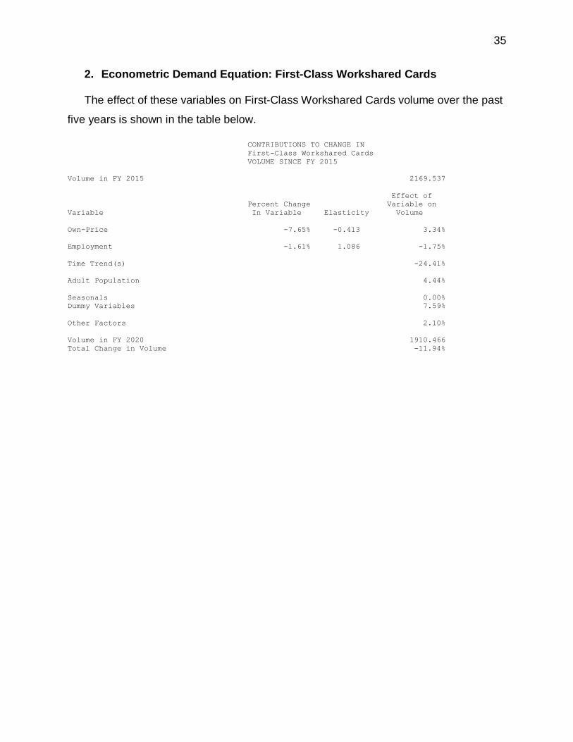
2. Econometric Demand Equation: First-Class Workshared Cards

The effect of these variables on First-Class Workshared Cards volume over the past



First-Class Workshared Cards


Volume in FY 2015 2169.537

Effect of



Own-Price -7.65% -0.413 3.34%

Employment -1.61% 1.086 -1.75%



Seasonals 0.00%


Other Factors 2.10%

Volume in FY 2020 1910.466


36

First-Class Workshared Flats

1. Explanatory Variables used in First-Class Workshared Flats Equation

The First-Class Workshared Flats demand equation includes the following



The relationship between First-Class Workshared Flats and the general economy is


variable in the First-Class Workshared Flats equation.

Employment is entered into the First-Class Workshared Flats equation with no lag.

(2) Postal Price

The First-Class Workshared Flats equation includes a single Postal price: the price

of First-Class Workshared Flats (PC01WS_F). Prices are entered current and lagged

one to two quarters.

(3) Time Trends

The First-Class Workshared Flats demand equation includes linear time trends

starting in 2008Q1 and 2017Q2. These trends reflect the impact of mail-diverting

technologies which have been continually adopted by businesses and households in

recent years.

(4) Other Variables

The First-Class Workshared Flats equation includes two dummy variables: D_R07,

equal to one since the implementation of R2006-1 rates in May 2007, zero earlier; and

D2020Q4, equal to one in 2020Q4 and zero elsewhere. The latter of these dummies is


37

Finally, the First-Class Workshared Flats equation includes a full-sample set of Q1

and Q2 seasonal variables, with an additional Q1 dummy since 2015Q1.

2. Econometric Demand Equation: First-Class Workshared Flats

The effect of these variables on First-Class Workshared Flats volume over the past



First-Class Workshared Flats



Effect of



Own-Price -17.91% -0.319 6.50%

Employment -1.61% 1.122 -1.81%



Seasonals 0.00%





38

Outbound First-Class International Letters, Cards, and Flats

1. Explanatory Variables used in Outbound First-Class International Letters, Cards, and Flats Equation

The Outbound First-Class International Letters, Cards, and Flats demand equation

includes the following explanatory variables.

(1) Macro-Economic Variable: Exports

The relationship between Outbound First-Class International Letters, Cards, and

Flats and the general economy is modeled through the inclusion of exports (XR) as an

explanatory variable in the Outbound First-Class International Letters, Cards, and Flats

demand equation. Exports are entered into the Outbound First-Class International

Letters, Cards, and Flats equation with no lag.

(2) Postal Price

The Outbound First-Class International Letters, Cards, and Flats equation includes a

single Postal price: the price of Outbound First-Class International Letters, Cards, and

Flats (PC1I_LCF). Prices are entered current only.

(3) Time Trend

The Outbound First-Class International Letters, Cards, and Flats equation includes a

full-sample linear time trend. This trend reflects the impact of mail-diverting technologies


(4) Other Variables

The Outbound First-Class International Letters, Cards, and Flats equation includes

five dummy variables: D2009Q2, which is equal to one in 2009Q2, zero elsewhere;

D2009Q3, equal to one in 2009Q3, zero elsewhere; D2009Q4, which is equal to one in

39

2009Q4, zero elsewhere; D2020Q3, equal to one in 2020Q3, zero elsewhere; and

D2020Q4, equal to one in 2020Q4, zero elsewhere. The latter two of these dummies

are included to capture the unique impact of recent events related to COVID-19.

The Outbound First-Class International Letters, Cards, and Flats equation also

includes a set of full-sample seasonal variables. with an additional Q1 dummy since

2013Q1.

2. Econometric Demand Equation: Outbound First-Class International Letters, Cards, and Flats

The effect of these variables on Outbound First-Class International Letters, Cards,

and Flats volume over the past five years is shown in the table below.


First-Class International Letters, Cards, & Flats



Effect of



Own-Price -6.71% -0.114 0.79%

Exchange Rate -8.14% 0.645 -5.33%




Seasonals 0.00%


Other Factors 3.32%



40

Marketing Mail

1. Overview of Direct-Mail Advertising

More than 90 percent of Marketing Mail can be characterized as direct-mail

advertising. Hence, understanding the demand for direct-mail advertising is the key to

understanding the demand for Marketing Mail volume.

The demand for Marketing Mail volume is the result of a choice by advertisers

regarding how much to spend on direct-mail advertising expenditures. The decision

process made by direct-mail advertisers can be decomposed into two separate, but

interrelated, decisions:

(1) How much to invest in advertising?

(2) Which advertising medium to use?

These two decisions are integrated into the demand equations associated with

Marketing Mail volume by including a set of explanatory variables in the demand

equations for Marketing Mail that addresses each of these decisions. These decisions,

and their implications for Marketing Mail equations, are considered separately below.

2. Advertising Decisions and Their Impact on Mail Volume

a. How Much to Invest in Advertising

Advertising represents a form of business investment. Hence, the Marketing Mail

equations include real gross private domestic investment as a measure of the overall

demand for business investment.

In addition to macroeconomic factors, the overall level of advertising is also affected

by certain other regular events. In the United States, the election cycle is one factor

which drives advertising demand. Variables which coincide with the timing of federal

elections are included in most of the Marketing Mail demand equations which were filed

with the Commission on January 21, 2020.

41

b. Which Advertising Media to Use

The choice of advertising media can be thought of as primarily a pricing decision, so

that the primary determinant of the demand for direct-mail advertising (vis-à-vis other

advertising media) would be the price of direct-mail advertising.

The most obvious way in which the price of direct-mail advertising is included in the

Marketing Mail equations is through the price of Marketing Mail. Postage costs are

included in the Marketing Mail equations through chain-weighted price indices which

measure the average postage paid by Marketing Mailers.

One of the principal advantages of direct-mail advertising over other forms of

advertising is that direct-mail advertising allows an advertiser to address customers on a

one-on-one basis. By identifying specifically who will receive a particular piece of direct-

mail advertising, direct-mail advertising is able to provide a level of targeting that is not

necessarily available through other advertising media.

The ability to target a direct mailing to specific individuals, based on specific

advertiser-chosen criteria, has increased dramatically. This had a positive impact on

the demand for many types of Marketing Mail. More recently, the emergence of Internet

and Mobile Advertising, often collectively referred to as digital advertising, have

negatively affected the demand for Marketing Mail as marketers have shifted spending

away from traditional forms of advertising. These factors are modeled via linear time

trends in several of the demand equations presented to the Commission this year.

Additional changes to the overall advertising market as well as direct mail’s role

within that market in the wake of the Great Recession are modeled via Intervention

analysis. The general concept of Intervention analysis was described earlier in this

document. The specific demand specifications associated with the demand equations

developed here for Marketing Mail are described below.

42

Marketing Mail Commercial Letters

1. Explanatory Variables used in Marketing Mail Commercial Letters Equation

The Marketing Mail Commercial Letters demand equation includes the following


(1) Macro-Economic Variable: Investment

The relationship between Marketing Mail Commercial Letters volume and the

general economy is modeled through the inclusion of gross private domestic investment

(INVR).

(2) Postal Price

The Marketing Mail Commercial Letters equation includes a price index measuring

the average price of Marketing Mail Commercial Letters (PC3R_NCR_L). Prices are

entered current and lagged one to four quarters.

(3) Time Trends

The Marketing Mail Commercial Letters demand equation includes a full-sample

linear time trend, a second linear time trend starting in 2011Q2, and a third linear time

trend starting in 2015Q2.

The full-sample trend is included to capture general increases in the attractiveness

of direct-mail advertising as a desirable advertising medium as well as in Marketing Mail

Commercial letters volume specifically relative to other direct-mail alternatives (e.g.,

ECR Basic Mail).

The second trend is introduced in 2011Q2 to capture the lingering economic impacts

of the Great Recession and increased electronic diversion due to the increased use of

43

new technologies such as smart phones and social media to the extent such usage led

to a decline in direct-mail advertising.

The third trend likely reflects increasing shifts of advertising from traditional media to

digital advertising.


The Great Recession hit advertising expenditures, and, hence, Marketing Mail

volume, much harder and more permanently than would have been expected, even

given the decline that occurred in private investment. To capture this effect

econometrically, the Marketing Mail Commercial Letters demand equation includes a

non-linear intervention variable that starts in 2008Q2 and takes the following form:




2008Q2 of ω0, which decays toward a long-run value of ω2.

(5) Other Variables

The Marketing Mail Commercial Letters equation includes several dummy variables

to reflect the impact of various one-time events and/or changes to the relative

relationship between Marketing Mail Commercial Letters and other mail categories.

(a) R2006-1

A dummy variable equal to one starting with the implementation of R2006-1 rates in

2007Q3 (D_R07) is included in the Marketing Mail Commercial Letters equation.

44

Commercial ECR automation letter discounts were eliminated at this time, leading this

mail to migrate from Commercial ECR Basic to Commercial Letters.

(b) 2012

A dummy variable, D2012Q1, equal to one in 2012Q1, zero otherwise, is included in

the Marketing Mail Commercial Letters equation. Another dummy variable,

D2012Q2ON, equal to one from 2012Q2 forward, zero otherwise, is also included.

(c) 2014

A dummy variable, D2014Q2ON, equal to one from 2014Q2 forward, zero otherwise,

is included in the Marketing Mail Commercial Letters equation to model possible level

change due to the separation of Political and Election (P&E) Mail from the rest of

Marketing Mail starting in 2014Q2.

(d) 2016 and 2017

A dummy variable, D2016Q1ON, equal to one from 2016Q1 forward, zero otherwise,

is included in the Marketing Mail Commercial Letters equation. Another dummy

variable, D2017Q1ON, equal to one from 2017Q1 forward, zero otherwise, is also

included.

(e) 2020

A dummy variable, D2020Q3, equal to one in 2020Q3, zero otherwise, and a dummy

variable, D2020Q4, equal to one in 2020Q4, zero otherwise, are included in the

Marketing Mail Commercial Letters equation. These dummies are included to capture

the unique impact of recent events related to COVID-19.

45

(f) Seasonal and Election Variables

Finally, the Marketing Mail Commercial Letters equation includes a set of seasonal

and election variables.

2. Econometric Demand Equation: Marketing Mail Commercial Letters The effect of these variables on Marketing Mail Commercial Letters volume over the



Mktg Mail: Commercial Letters (non-P&E)


Volume in FY 2015 38048.111

Effect of



Own-Price -4.14% -0.540 2.31%

Investment -0.39% 0.409 -0.16%


Non-Linear Intervention Starting in 2008Q2 -0.00%



Seasonals 0.00%

Elections 0.00%

Dummy Variablesc 2.15%

Other Factors 1.26%

Volume in FY 2020 29133.110


46

Marketing Mail Commercial High Density and Saturation Letters

1. Explanatory Variables used in Marketing Mail Commercial High Density and Saturation Letters Equation

The Marketing Mail Commercial High Density and Saturation Letters demand

equation includes the following explanatory variables.


The relationship between Marketing Mail Commercial High Density and Saturation

Letters volume and the general economy is modeled through the inclusion of gross

private domestic investment (INVR).

(2) Postal Price

The Marketing Mail Commercial High Density and Saturation Letters equation

contains a price index for the price of Marketing Mail Commercial High Density and

Saturation Letters (PC3R_HS_L). Prices are entered current and lagged one quarter.

(3) Time Trends

The Marketing Mail Commercial High Density and Saturation Letters demand

equation includes a linear time trend starting in 2014Q4 and a second linear time trend

starting in 2016Q4.

(4) Other Variables



Marketing Mail Commercial High Density and Saturation Letters equation. These

47

dummies are included to capture the unique impact of recent events related to COVID-

19.

The Marketing Mail Commercial High Density and Saturation Letters equation also

includes a set of seasonal variables.

2. Econometric Demand Equation: Marketing Mail Commercial High Density and Saturation Letters

The effect of these variables on Marketing Mail Commercial High Density and

Saturation Letters volume over the past five years is shown in the table below.


Mktg Mail: Comm High-D/Saturation Letters (non-P&E)


Volume in FY 2015 5638.145

Effect of



Own-Price -2.12% -0.586 1.27%

Investment -0.39% 0.711 -0.28%


Time Trend(s) 2.88%


Seasonals 0.42%

Other Factors 0.25%

Volume in FY 2020 5862.246

Total Change in Volume 3.97%

48

Marketing Mail Commercial and ECR Basic Flats

1. Explanatory Variables used in Marketing Mail Commercial and ECR Basic Flats Equation

The Marketing Mail Commercial and ECR Basic Flats demand equation includes the



The relationship between Marketing Mail Commercial and ECR Basic Flats volume

and the general economy is modeled through the inclusion of gross private domestic

investment (INVR). Investment is entered without lag. The coefficient on investment is

stochastically constrained from a Marketing Mail Commercial and ECR Basic Flats

equation with investment lagged two quarters and estimated through 2020Q1.

(2) Postal Price

The Marketing Mail Commercial and ECR Basic Flats equation includes a price

index measuring the average price of Marketing Mail Commercial and ECR Basic Flats.

Prices are entered current and lagged one to two quarters. The coefficient on postal

price is stochastically constrained from a Marketing Mail Commercial and ECR Basic

Flats equation with investment lagged two quarters and estimated through 2020Q1.

(3) Time Trends

The Marketing Mail Commercial and ECR Basic Flats equation includes a full-

sample linear time trend and a second linear time trend starting in 2016Q4.

49

(4) Other Variables

The Marketing Mail Commercial and ECR Basic Flats equation includes one non-

seasonal dummy variable, D2019Q2ON, equal to one from 2019Q2 forward, zero

otherwise.



Marketing Mail Commercial and ECR Basic Flats equation. These dummies are


Finally, the Marketing Mail Commercial and ECR Basic Flats equation includes a set

of seasonal and election variables.

50

2. Econometric Demand Equation: Marketing Mail Commercial and ECR Basic Flats

The effect of these variables on Marketing Mail Commercial and ECR Basic Flats

volume over the past five years is shown in the table below.


Mktg Mail: Commercial Flats & ECR Basic (non-P&E)


Volume in FY 2015 11444.396

Effect of



Own-Price -1.97% -0.305 0.61%

Investment -0.39% 0.280 -0.11%




Seasonals 0.00%

Elections 0.00%


Other Factors 4.31%

Volume in FY 2020 6451.599


51

Marketing Mail Commercial High Density and Saturation Flats

1. Explanatory Variables used in Marketing Mail Commercial High Density and Saturation Flats Equation

The Marketing Mail Commercial High Density and Saturation Flats demand equation



The relationship between Marketing Mail Commercial High Density and Saturation

Flats volume and the general economy is modeled through the inclusion of gross private

domestic investment (INVR).

(2) Postal Price

The Marketing Mail Commercial High Density and Saturation Flats equation contains

a price index measuring the average price of Marketing Mail Commercial High Density

and Saturation Flats. Prices are entered current and lagged one to two quarters.

(3) Time Trend

The Marketing Mail Commercial High Density and Saturation Flats demand equation

includes a linear time trend starting in 2015Q3.

(4) Other Variables

The Marketing Mail Commercial High Density and Saturation Flats equation includes

three non-seasonal dummy variables: D2014Q2ON, equal to one from 2014Q2 forward,

zero otherwise, to model possible level change due to the separation of Political and

Election (P&E) Mail from the rest of Marketing Mail starting in 2014Q2; and D2020Q3

and D2020Q4, which are equal to one in 2020Q3 and 2020Q4, respectively, zero

52

otherwise. The latter two of these dummies are included to capture the unique impact of

recent events related to COVID-19.

Finally, the Marketing Mail Commercial High Density and Saturation Flats equation

includes a set of seasonal and election variables.

2. Econometric Demand Equation: Marketing Mail Commercial High Density and Saturation Flats

The effect of these variables on Marketing Mail Commercial High Density and

Saturation Flats volume over the past five years is shown in the table below.


Mktg Mail: Comm High-D/Saturation Flats (non-P&E)


Volume in FY 2015 10731.782

Effect of



Own-Price -7.69% -0.443 3.61%

Investment -0.39% 0.233 -0.09%




Seasonals 0.00%

Elections 0.00%


Other Factors 0.53%

Volume in FY 2020 9543.281


53

Marketing Mail Commercial Every Door Direct Mail (EDDM)

1. Explanatory Variables used in EDDM Equation

The Marketing Mail EDDM demand equation includes the following explanatory

variables.


The relationship between Marketing Mail EDDM volume and the general economy is

modeled through the inclusion of gross private domestic investment (INVR).

(2) Postal Price

The Marketing Mail EDDM equation contains a price index for the price of Marketing

Mail EDDM (PC3R_ED). Prices are entered current and lagged one quarter.

(3) Time Trend

The Marketing Mail EDDM demand equation includes a linear time trend starting in

2014Q3.

(4) Other Variables

The Marketing Mail EDDM equation includes four non-seasonal dummy variables:

D2014Q4, which is equal to one in 2014Q4 and zero otherwise; D2016Q1ON, which is

equal to one starting in 2016Q1 and zero before that time; and D2020Q3 and D2020Q4,

which are equal to one in 2020Q3 and 2020Q4, respectively, zero otherwise. The latter

two of these dummies are included to capture the unique impact of recent events

related to COVID-19.

Finally, the Marketing Mail EDDM equation includes a set of seasonal variables.

54

2. Econometric Demand Equation: Marketing Mail EDDM

The effect of these variables on Marketing Mail EDDM volume over the past five

years is shown in the table below.


Every Door Direct Mail (non-P&E)



Effect of



Own-Price -1.50% -0.394 0.60%

Investment -0.39% 0.887 -0.35%



Seasonals 0.00%





55

Marketing Mail Nonprofit Letters

1. Explanatory Variables used in Marketing Mail Nonprofit Letters Equation

The Marketing Mail Nonprofit Letters demand equation includes the following



The relationship between Marketing Mail Nonprofit Letters volume and the general

economy is modeled through the inclusion of gross private domestic investment (INVR).

(2) Postal Price

The Marketing Mail Nonprofit Letters equation contains a price index for the price of

Marketing Mail Nonprofit Letters (PC3N_NCR_L). Prices are entered current and

lagged one to two quarters.

(3) Time Trends

The Marketing Mail Nonprofit Letters equation includes a full-sample linear time

trend and a Q1 seasonal trend which is a full-sample linear time trend multiplied by the

Q1 seasonal dummy.

(5) Other Variables

The Marketing Mail Nonprofit Letters equation includes several dummy variables.

(a) R2006-1

A dummy variable equal to one starting with the implementation of R2006-1 rates in

2007Q3 (D_R07) is included in the Marketing Mail Nonprofit Letters equation. D_R07 is

included current and lagged two quarters.

56

(b) D_R11

A dummy variable equal to one since the Postal Service’s April 2011, rate change

(2011Q3) is included in the Marketing Mail Nonprofit Letters equation.

(c) D_R13

A dummy variable equal to one since the Postal Service’s January 2013, rate

change (2013Q2) is included in the Marketing Mail Nonprofit Letters equation.

(d) 2020

The dummy variable, D2020Q3, which is equal to one in 2020Q3, zero otherwise, is

included in the Marketing Mail Nonprofit Letters equation. This dummy variable is


(e) Seasonal and Election Variables

Finally, the Marketing Mail Nonprofit Letters equation includes a set of seasonal and

election variables.

57

2. Econometric Demand Equation: Marketing Mail Nonprofit Letters

The effect of these variables on Marketing Mail Nonprofit Letters volume over the



Mktg Mail: Nonprofit Letters (non-P&E)


Volume in FY 2015 9153.990

Effect of



Own-Price -2.75% -0.351 0.98%

Investment -0.39% 0.318 -0.13%



Seasonals 0.91%

Elections 0.00%


Other Factors 1.78%

Volume in FY 2020 8361.075


58

Marketing Mail Nonprofit High Density and Saturation Letters

1. Explanatory Variables used in Marketing Mail Nonprofit High Density and Saturation Letters Equation

Marketing Mail Nonprofit High Density and Saturation Letters demand equation



The relationship between Marketing Mail Nonprofit High Density and Saturation

Letters volume and the general economy is modeled through the inclusion of gross

private domestic investment (INVR).

(2) Postal Price

The Marketing Mail Nonprofit High Density and Saturation Letters equation contains

a price index for the price of Marketing Mail Nonprofit High Density and Saturation

Letters (PC3N_HS_L). Prices are entered current only.

(3) Time Trend

The Marketing Mail Nonprofit High Density and Saturation Letters equation includes

a linear time trend starting in 2017Q2.

(4) Other Variables


a dummy variable, D2014Q2ON, equal to one from 2014Q2 forward, zero otherwise, to

model possible level change due to the separation of Political and Election (P&E) Mail

from the rest of Marketing Mail starting in 2014Q2.

59

The Marketing Mail Nonprofit High Density and Saturation Letters equation also

includes several other dummy variables: D2011Q1ON, equal to one since 2011Q1, zero

elsewhere; D2015Q3ON, equal to one since 2015Q3, zero elsewhere; and

D2017Q2ON, equal to one since 2017Q2, zero elsewhere.


D2020Q3 and D2020Q4, which are equal to one in 2020Q3 and 2020Q4, respectively,

zero otherwise. These dummies are included to capture the unique impact of recent

events related to COVID-19.

Finally, the Marketing Mail Nonprofit High Density and Saturation Letters equation

includes a set of seasonal variables.

60

2. Econometric Demand Equation: Marketing Mail Nonprofit High Density and Saturation Letters

The effect of these variables on Marketing Mail Nonprofit High Density and

Saturation Letters volume over the past five years is shown in the table below.


Mktg Mail: NP High-D/Saturation Letters (non-P&E)



Effect of



Own-Price 0.09% -0.744 -0.07%

Investment -0.39% 0.531 -0.21%



Seasonals 0.00%


Other Factors 2.59%



61

Marketing Mail Nonprofit and ECR Basic Flats

1. Explanatory Variables used in Marketing Mail Nonprofit and ECR Basic Flats Equation

The Marketing Mail Nonprofit and ECR Basic Flats demand equation includes the



The relationship between Marketing Mail Nonprofit and ECR Basic Flats volume and

the general economy is modeled through the inclusion of gross private domestic

investment (INVR).

(2) Postal Price

The Marketing Mail Nonprofit and ECR Basic Flats equation contains a price index

for the price of Marketing Mail Nonprofit and ECR Basic Flats. Prices are entered

current only.

(3) Time Trend

The Marketing Mail Nonprofit and ECR Basic Flats equation includes a full-sample

linear time trend.

(4) Other Variables

The Marketing Mail Nonprofit and ECR Basic Flats equation includes a dummy

variable, D2014Q2ON, equal to one from 2014Q2 forward, zero otherwise, to model

possible level change due to the separation of Political and Election (P&E) Mail from the

rest of Marketing Mail starting in 2014Q2.

The Marketing Mail Nonprofit and ECR Basic Flats equation also includes several

other dummy variables: D2013Q1, which is equal to one in 2013Q1, zero elsewhere;

62

D2017Q1, which is equal to one in 2017Q1, zero elsewhere; and D2019Q2ON, which is

equal to one from 2019Q2 forward, zero otherwise.

The Marketing Mail Nonprofit and ECR Basic Flats equation also includes D2020Q3

and D2020Q4, which are equal to one in 2020Q3 and 2020Q4, respectively, zero

otherwise. These dummies are included to capture the unique impact of recent events


Finally, the Marketing Mail Nonprofit and ECR Basic Flats equation includes a set of

seasonal and election variables.

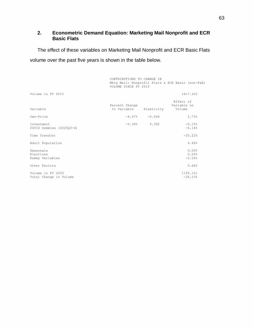
63

2. Econometric Demand Equation: Marketing Mail Nonprofit and ECR Basic Flats

The effect of these variables on Marketing Mail Nonprofit and ECR Basic Flats



Mktg Mail: Nonprofit Flats & ECR Basic (non-P&E)


Volume in FY 2015 1617.322

Effect of



Own-Price -4.67% -0.564 2.73%

Investment -0.39% 0.392 -0.15%




Seasonals 0.00%

Elections 0.00%


Other Factors 0.66%

Volume in FY 2020 1193.101


64

Marketing Mail Nonprofit High Density and Saturation Flats

1. Explanatory Variables used in Marketing Mail Nonprofit High Density and Saturation Flats Equation

Marketing Mail Nonprofit High Density and Saturation Flats demand equation



The relationship between Marketing Mail Nonprofit High Density and Saturation Flats

volume and the general economy is modeled through the inclusion of gross private

domestic investment (INVR).

(2) Postal Price

The Marketing Mail Nonprofit High Density and Saturation Flats equation contains a

price index for the price of Marketing Mail Nonprofit High Density and Saturation Flats.

Prices are entered current and lagged one to four quarters.

(3) Other Variables

The Marketing Mail Nonprofit High Density and Saturation Flats equation includes

five non-seasonal dummy variables: D2005Q2ON, equal to one since 2005Q2, zero

elsewhere; D2006Q2ON, equal to one since 2006Q2, zero elsewhere; D2016Q3ON,

equal to one since 2016Q3, zero elsewhere; and D2020Q3 and D2020Q4, which are

equal to one in 2020Q3 and 2020Q4, respectively, zero otherwise. The last two of these


19.

Finally, the Marketing Mail Nonprofit High Density and Saturation Flats equation

includes a set of seasonal and election variables.

65

2. Econometric Demand Equation: Marketing Mail Nonprofit High Density and Saturation Flats

The effect of these variables on Marketing Mail Nonprofit High Density and

Saturation Flats volume over the past five years is shown in the table below.


Mktg Mail: NP High-D/Saturation Flats (non-P&E)



Effect of



Own-Price -8.99% -0.923 9.07%

Investment -0.39% 0.127 -0.05%



Seasonals -3.65%

Elections 0.00%


Other Factors 7.26%



66

Commercial Marketing Political and Election Mail

1. Explanatory Variables used in Commercial Marketing Political and Election Mail Equation

Commercial Marketing Political and Election Mail demand equation includes the


(1) Postal Price

The Commercial Marketing Political and Election Mail equation includes average

revenue per piece for Commercial Marketing Political and Election Mail (RPP3R_PE) as

a measure of the average price of Commercial Marketing Political and Election Mail.

Prices are entered current only.

(2) Time Trend

The Commercial Marketing Political and Election Mail equation includes a full-

sample linear time trend.

(3) Dummy Variable related to the COVID-19 Pandemic

The impact of the COVID-19 pandemic on Commercial Marketing Political and

Election Mail volume is modeled through the inclusion of one dummy variable,

D2020Q3, equal to one in 2020Q3, zero otherwise.

(4) Other Variables

Finally, the Commercial Marketing Political and Election Mail equation includes a set

of seasonal and election variables.

67

2. Econometric Demand Equation: Commercial Marketing Political and Election Mail

The effect of these variables on Commercial Marketing Political and Election Mail



Commercial Marketing P&E Mail



Effect of



Own-Price -8.31% -0.594 5.29%

Time Trend(s) 38.53%


Seasonals 0.00%

Elections 97.50%


Volume in FY 2020 1309.709


68

Nonprofit Marketing Political and Election Mail

1. Explanatory Variables used in Nonprofit Marketing Political and Election Mail Equation

Nonprofit Marketing Political and Election Mail demand equation includes the


(1) Postal Price

The Nonprofit Marketing Political and Election Mail equation includes average

revenue per piece for Nonprofit Marketing Political and Election Mail (RPP3N_PE) as a

measure of the average price of Nonprofit Marketing Political and Election Mail. Prices

are entered current only.

(2) Time Trend

The Nonprofit Marketing Political and Election Mail equation includes a full-sample

linear time trend.

(3) Dummy Variable related to the COVID-19 Pandemic

The impact of the COVID-19 pandemic on Nonprofit Marketing Political and Election

Mail volume is modeled through the inclusion of one dummy variable, D2020Q3, equal

to one in 2020Q3, zero otherwise.

(4) Other Variables

Finally, the Nonprofit Marketing Political and Election Mail equation includes a set of

seasonal and election variables.

69

2. Econometric Demand Equation: Nonprofit Marketing Political and Election Mail

The effect of these variables on Nonprofit Marketing Political and Election Mail



Nonprofit Marketing P&E Mail



Effect of



Own-Price -7.00% -0.097 0.71%



Seasonals 0.00%

Elections 115.40%




70

Marketing Parcels

1. Explanatory Variables used in the Marketing Parcels Equation

The Marketing Parcels demand equation includes the following explanatory

variables.


The relationship between Marketing Parcels volume and the general economy is

modeled through the inclusion of gross private domestic investment (INVR).

(2) Postal Price

The Marketing Parcels demand equation includes a price index measuring the

average price of Marketing Parcels (PC3_P). Prices are entered current only.

(3) Time Trend

The Marketing Parcels equation includes a full-sample linear time trend.

(4) Other Variables

The Marketing Parcels equation includes several dummy variables: D_R12, equal to

one since the implementation of new rates in January 2012 (2012Q2), zero elsewhere;

D2016Q1ON, equal to one from 2016Q1 forward, zero otherwise; and D2019Q2ON,

equal to one from 2019Q2 forward, zero otherwise.

Finally, the Marketing Parcels equation includes a set of seasonal variables.

71

2. Econometric Demand Equation: Marketing Parcels

The effect of these variables on Marketing Parcels volume over the past five years

is shown in the table below.


Marketing Parcels



Effect of



Own-Price 0.56% -1.293 -0.72%

Investment -0.39% 0.376 -0.15%



Seasonals 0.00%


Other Factors 0.04%



72

Periodicals Mail

The Periodicals Mail class is available for mail that is sent at regular intervals and

contains at least a minimum level of editorial (i.e., non-advertising) content. This

type of mail may include magazines, newspapers, journals, and newsletters. The

Periodicals Mail class is divided into four subclasses, Periodicals Regular and three

subclasses which offer preferred rates for certain eligible mailers. In-County

Periodicals Mail is open to Periodicals which are sent within the same county as they

are printed. Periodicals Nonprofit mail is open to Periodicals sent by qualified not-

for-profit organizations. Periodicals Classroom mail is open to Periodicals sent to

educational institutions for educational purposes. The latter two of these subclasses

are combined within a single demand equation.

1. Factors Affecting Demand for Periodicals

The demand for Periodicals Mail is a derived demand, which is derived from the

demand of consumers for magazines and newspapers. Those factors which

influence the demand for newspapers and magazines would therefore be expected

to be the principal drivers of the demand for Periodicals Mail.

The factors which would be expected to influence the demand for newspapers and

magazines are drawn from basic micro-economic theory. These factors include the

state of the overall economy, the price of periodicals, and the demand for goods which

may serve as substitutes for newspapers and magazines.

The Periodicals demand equations include total private employment. Employment

works better econometrically at explaining Periodicals Mail volumes than other macro-

economic variables tested, including personal disposable income, consumption

expenditures, and retail sales.

The price of periodicals is measured by the price of postage paid by publishers (and

paid implicitly by consumers through subscription rates). In addition to affecting the

73

price of newspapers and magazines by being incorporated into subscription rates, the

price charged by the Postal Service will also affect the demand for Periodicals Mail

directly by affecting publishers’ decisions over how to deliver their Periodicals. For

example, the delivery requirements of many weekly newspapers can be satisfied by

either mail or private delivery.

The Periodicals demand equations used here also include long-run time trends.

These trends are the result of long-run shifts away from reading. In addition to the full-

sample linear time trend, an additional negative trend is also included in the Periodical

Regular demand equation to account for more recent declines in Periodicals Mail

volume due to increased substitution faced by Periodicals from the Internet, mobile

devices, and e-readers.

74

Periodical Regular Mail

1. Explanatory Variables used in Periodical Regular Mail Equation The Periodical Regular Mail demand equation includes the following explanatory

variables.


The relationship between Periodical Regular Mail and the general economy is


variable in the Periodicals Regular Mail equation.

(2) Postal Price

The Periodical Regular Mail demand equation includes a price index measuring the

average price of Periodicals Regular Mail (PC2R). Prices are entered current and

lagged one quarter.

(3) Time Trends

The Periodical Regular Mail demand equation includes a full-sample linear time

trend, a linear time trend starting in 2011Q2, and a linear time trend starting in 2017Q4.

The full-sample time trend reflects the general decline in reading that has contributed to

a reduction in Periodicals Mail volumes for many years. The latter time trends reflect

the additional decline in volume due to the emergence of online alternatives to printed

magazines and newspapers.

75


The Periodical Regular Mail demand equation includes a non-linear intervention

variable that starts in 2007Q4 and takes the following form:




2007Q4 of ω0, which decays toward a long-run value of ω2. This variable measures the

unique impact of the Great Recession on Periodical Regular Mail volume.

(5) Other Variables

The Periodical Regular Mail equation also includes a set of seasonal variables.

76

2. Econometric Demand Equation: Periodical Regular Mail

The effect of these variables on Periodical Regular Mail volume over the past five



Periodical Regular Mail


Volume in FY 2015 3851.202

Effect of



Own-Price -4.55% -0.130 0.61%

Employment -1.61% 1.138 -1.83%

Non-Linear Intervention starting in:

2007Q4 -3.15%



Seasonals 1.81%


Volume in FY 2020 2356.757


77

Periodicals Nonprofit and Classroom

A single demand equation is estimated for Periodicals Nonprofit and Classroom

mail.

1. Explanatory Variables used in Periodicals Nonprofit and Classroom Mail Equation

The Periodicals Nonprofit and Classroom Mail demand equation includes the



The relationship between Periodicals Nonprofit and Classroom Mail and the general


explanatory variable in the Periodicals Nonprofit and Classroom Mail equation.

(2) Postal Price

The Periodicals Nonprofit and Classroom Mail demand equation includes a price

index measuring the average price of Periodicals Nonprofit and Classroom Mail

(PC12_13). Prices are entered current and lagged one to four quarters.

(3) Time Trend

The Periodicals Nonprofit and Classroom Mail demand equation includes a full-

sample linear time trend.

(4) Other Variables

The Periodicals Nonprofit and Classroom Mail equation includes three non-seasonal

dummy variables: D2016Q3ON, which is equal to one from 2016Q3 onward, zero prior

to 2016Q3; D2018Q2, equal to one in 2018Q2, zero elsewhere; and D2018Q3, equal to

one in 2018Q3, zero elsewhere.

78

Finally, the Periodicals Nonprofit and Classroom Mail equation includes a set of

seasonal variables.

2. Econometric Demand Equation: Periodicals Nonprofit and Classroom Mail

The effect of these variables on Periodicals Nonprofit and Classroom Mail volume



Periodical Nonprofit & Classroom


Volume in FY 2015 1416.156

Effect of



Own-Price -3.19% -0.283 0.92%

Employment -1.61% 0.186 -0.30%



Seasonals 0.00%



Volume in FY 2020 1179.960


79

Periodicals Within County Mail

1. Explanatory Variables used in Periodicals Within County Mail Equation The Periodicals Within County Mail demand equation includes the following



The relationship between Periodicals Within County Mail and the general economy


variable in the Periodicals Within County Mail equation.

(2) Postal Price

The Periodicals Within County Mail demand equation includes a price index

measuring the average price of Periodicals Within County Mail. Prices are entered

current only with no lags.

(3) Time Trend

The Periodicals Within County Mail demand equation includes a full-sample linear

time trend as well as a second linear time trend starting in 2019Q1.

(4) Other Variables

The Periodicals Within County demand equation includes one non-seasonal dummy

variables: D2016Q4_17Q1, which is equal to one in 2016Q4 and 2017Q1, zero

elsewhere.

Finally, the Periodicals Within County Mail equation includes a set of seasonal

variables.

80

2. Econometric Demand Equation: Periodicals Within County Mail The effect of these variables on Periodicals Within County Mail volume over the past



Periodical Within-County



Effect of



Own-Price -5.70% -0.186 1.10%

Employment -1.61% 0.903 -1.46%



Seasonals 0.00%





81

Package Delivery Services

Package delivery services refer broadly to the delivery of goods other than

Periodicals, advertisements, and correspondence. Examples of this type of mail include

mail-order deliveries such as clothes or books, as well as packages sent by households

(e.g., Christmas presents). Among market-dominant mail categories, this encompasses

Marketing parcels, which were discussed earlier, and the Package Services mail class.

The demand for package delivery services will be largely driven by the demand for

the goods being delivered. In the cases of most package delivery services, this

relationship is modeled through the inclusion of e-commerce sales as an explanatory

variable.

Most Package Delivery Services face significant competition from other delivery

firms, including United Parcel Service and Federal Express. Because of this, most

categories of mail that can best be described as Package Delivery Services are

classified as competitive mail products and are not included as part of this report.

As of January 2021, there were four market-dominant subclasses of mail in the

Package Services class: Alaska Bypass, Bound Printed Matter (BPM) Flats, BPM

Parcels, and Media and Library Rate Mail.

The specific demand equations for Market-Dominant Package Delivery Services are

presented in more detail below.

82

Alaska Bypass

1. Explanatory Variables used in the Alaska Bypass Equation

The Alaska Bypass demand equation includes the following explanatory variables.

(1) Macro-Economic Variable: Non-Farm Alaska Employment

The relationship between Alaska Bypass volume and the economy is modeled

through the inclusion of Alaska non-farm employment (EMPL_AK) as an explanatory

variable in the Alaska Bypass demand equation.

(2) Postal Price

The Alaska Bypass demand equation includes a price index for the average price of

Alaska Bypass (PC25_AB). Prices are entered current only.

(3) Time Trend

The Alaska Bypass equation includes a linear time trend starting in 2018Q1.

(4) Other Variables

The Alaska Bypass equation includes three dummy variables: D2019Q1, equal to

one in 2019Q1, zero elsewhere; D2020Q3, equal to one in 2020Q3, zero elsewhere;

and D2020Q4, equal to one in 2020Q4, zero elsewhere. The latter two of these


19.

Finally, the Alaska Bypass equation includes a set of seasonal variables.

83

2. Econometric Demand Equation: Alaska Bypass

The effect of these variables on Alaska Bypass volume over the past five years is

shown in the table below.


Alaska Bypass



Effect of



Own-Price -5.48% -0.271 1.54%

Employment (Alaska) -12.47% 0.596 -7.63%




Seasonals 0.00%





84

Bound Printed Matter Flats

1. Explanatory Variables used in Bound Printed Matter Flats Equation

The Bound Printed Matter Flats demand equation includes the following explanatory

variables.


The relationship between Bound Printed Matter Flats volume and the general

economy is modeled through the inclusion of gross private domestic investment (INVR).

(2) Postal Price

The Bound Printed Matter Flats equation includes a price index measuring the

average price of Bound Printed Matter Flats (PC28_F). Prices are entered current and

lagged one to two quarters.

(3) Time Trend

The Bound Printed Matter Flats equation includes a linear time trend starting in

2017Q3.

(4) Other Variables

The Bound Printed Matter Flats equation includes two dummy variables: D2016Q1,

which is equal to one in 2016Q1, zero elsewhere; and D2020Q4, which is equal to one

in 2020Q4, zero elsewhere. The latter of these dummies is included to capture the


Finally, the Bound Printed Matter Flats equation includes a set of seasonal variables.

85

2. Econometric Demand Equation: Bound Printed Matter Flats

The effect of these variables on Bound Printed Matter Flats volume over the past



Bound Printed Matter Flats



Effect of



Own-Price -6.40% -0.718 4.86%

Investment -0.39% 0.780 -0.31%

COVID Dummy (2020Q4) -6.75%



Seasonals -4.97%





86

Bound Printed Matter Parcels

1. Explanatory Variables used in Bound Printed Matter Parcels Equation The Bound Printed Matter Parcels demand equation includes the following


(1) Macro-Economic Variable: E-Commerce

The Bound Printed Matter Parcels equation includes e-commerce retail sales

(ECOMM) to model the relationship between package volumes and online shopping.

(2) Postal Price

The Bound Printed Matter Parcels demand equation includes a price index

measuring the average price Bound Printed Matter Parcels (PC28_P). Prices are

entered current only.

(3) Time Trend

The Bound Printed Matter Parcels demand equation includes a full sample, linear

time trend.


The Bound Printed Matter Parcels demand equation includes a non-linear s-curve

starting in 2014Q3.

87

(5) Other Variables

The Bound Printed Matter Parcels equation includes one dummy variable:

D2019Q4ON, equal to one since 2019Q4, zero elsewhere.

Finally, the Bound Printed Matter Parcels equation includes a set of seasonal

variables.

2. Econometric Demand Equation: Bound Printed Matter Parcels The effect of these variables on Bound Printed Matter Parcels volume over the past



Bound Printed Matter Parcels



Effect of



Own-Price -5.19% -0.516 2.79%

E-Commerce Sales 94.50% 0.602 49.29%



Non-Linear Intervention Starting in:

2014Q3 58.46%

Seasonals 0.00%





88

Media and Library Rate Mail

1. Explanatory Variables used in Media and Library Rate Mail Equation The Media and Library Rate Mail demand equation includes the following


(1) Macro-Economic Variable: E-Commerce

The Media and Library Rate Mail equation includes e-commerce retail sales

(ECOMM) to model the relationship between package volumes and online shopping.

The coefficient on e-commerce sales is constrained to a value one (1.0) in the Media

and Library Rate Mail demand equation.

(2) Postal Price

The Media and Library Rate mail equation includes the price of Media and Library

Rate Mail (PC29_30). Prices are entered current and lagged one to four quarters.

(3) Time Trends

The Media and Library Rate Mail demand equation includes a full-sample linear time

trend, and a second linear time trend starting in 2015Q4.

(4) Other Variables

The Media and Library Rate Mail equation includes three dummy variables:

D2020Q2, equal to one in 2020Q2, zero elsewhere; D2020Q3, equal to one in 2020Q3,

zero elsewhere; and D2020Q4, equal to one in 2020Q4, zero elsewhere. These


19.

Finally, the Media and Library Rate Mail equation includes a set of seasonal

variables.

89

2. Econometric Demand Equation: Media and Library Rate Mail

The effect of these variables on Media and Library Rate Mail volume over the past



Media and Library Rate



Effect of



Own-Price -2.99% -0.676 2.07%

E-Commerce Sales 94.50% 1.000 94.50%

COVID Dummies (2020Q2-4) 42.72% 0.066 8.39%



Seasonals 1.62%

Other Factors 0.46%



90

Free Mail Services

There are two mail categories for which mail is free to the sender: Postal Penalty

Mail, mail sent by the Postal Service; and Free-for-the-Blind Mail, which is free for blind

or handicapped consumers. Because these mail categories are free, Postal prices are

not included as explanatory variables in these equations. The specific demand

equations used to model Postal Penalty and Free-for-the-Blind mail volumes are

outlined below.

Postal Penalty Mail

1. Explanatory Variables used in Postal Penalty Mail Equation The Postal Penalty Mail demand equation includes the following explanatory

variables.

(1) Time Trend

The Postal Penalty equation includes a full-sample linear time trend.

(2) Other Variables

The Postal Penalty Mail equation also includes two dummy variables: D2013Q4,

equal to one in 2013Q4, zero elsewhere; D2020Q4, equal to one in 2020Q4, zero

elsewhere. The latter of these dummies is included to capture the unique impact of

recent events related to COVID-19.

Finally, the Postal Penalty equation includes a set of seasonal variables.

91

2. Econometric Demand Equation: Postal Penalty Mail The effect of these variables on Postal Penalty Mail volume over the past five years



Postal Penalty



Effect of





Seasonals -18.01%





92

Free-for-the-Blind and Handicapped Mail

1. Explanatory Variables used in Free-for-the-Blind Mail Equation The Free-for-the-Blind Mail demand equation includes the following explanatory

variables.

(1) Time Trend

The Free-for-the-Blind Mail equation includes a full-sample linear time trend and a

second linear time trend starting in 2018Q4.

(2) Other Variables

The Free-for-the-Blind Mail equation also includes two dummy variables: D2020Q3,

equal to one in 2020Q3, zero elsewhere; D2020Q4, equal to one in 2020Q4, zero

elsewhere. These dummies are included to capture the unique impact of recent events


2. Econometric Demand Equation: Free-for-the-Blind Mail The effect of these variables on Free-for-the-Blind Mail volume over the past five



Free-for-the-Blind



Effect of






Seasonals 0.00%

Other Factors 4.96%



93

Ancillary and Special Services

General Overview

Ancillary services are not mail volumes but represent add-ons to mail volumes. That

is, a certified letter would be counted as both a piece of Certified Mail as well as a First-

Class Letter. Therefore, the volumes of ancillary services are not included in a

calculation of total Postal Service volume.

Because ancillary services are add-ons to existing mail volumes, the demand for

ancillary services may be affected directly by the demand for complementary categories

of mail. For example, the volume of Stamped Envelopes is modeled in part as a

function of the volume of First-Class Single-Piece Letters since all Stamped Envelopes

are, in fact, First-Class Single-Piece Letters.

Special services are not add-ons to mail volumes but represent separate volume.

Special service volumes are not generally viewed as “mail” volume per se. Econometric

demand equations are estimated for two special services: Money Orders and Post

Office Boxes.

The ancillary and special service volumes modeled here have generally exhibited

long-run trends. For this reason, a time trend is included in the demand equation

associated with most of these services.

Finally, the demand for ancillary and special services is also a function of the price

charged by the Postal Service for these services. In addition, most of the ancillary and

special service equations also include some equation-specific variables, which are

described below.

Specific demand equations for ancillary and special services are described in detail

below.

94

Registered Mail

1. Explanatory Variables used in Registered Mail Equation The Registered Mail demand equation includes the following explanatory variables.

(1) Postal Price

The Registered Mail equation includes a price index measuring the average price of

Registered Mail (PC35). Prices are entered current and lagged one to four quarters.

(2) Time Trend

The Registered Mail equation includes a full-sample linear time trend, and a second

linear time trend starting in 2017Q3.

(3) Other Variables

The Registered Mail equation contains two non-seasonal dummy variables:


zero elsewhere.

The Registered Mail equation also includes a set of seasonal variables.

95

2. Econometric Demand Equation: Registered Mail The effect of these variables on Registered Mail volume over the past five years is



Registered



Effect of



Own-Price -4.16% -1.118 4.87%



Seasonals 0.00%





96

Insured Mail

1. Explanatory Variables used in Insured Mail Equation The Insured Mail demand equation includes the following explanatory variables.

(1) Postal Price

The Insured Mail equation includes a price index measuring the average price of

Insured Mail (PC36). Prices are entered current and lagged one to four quarters.

(2) Time Trend

The Insured Mail equation includes a full-sample linear time trend, and a second

linear time trend starting in 2017Q3.

(3) Other Variables

The Insured Mail equation includes five dummy variables: D_FREEINS, which is set

equal to one since the introduction of free insurance attached to Priority Mail, in the

fourth Postal Quarter of FY 2013; D2015Q4, equal to one in 2015Q4, zero elsewhere;


zero elsewhere; and D2020Q4, equal to one in 2020Q4, zero elsewhere. The latter two

of these dummies are included to capture the unique impact of recent events related to

COVID-19.

Finally, the Insured Mail equation includes a set of seasonal variables.

97

2. Econometric Demand Equation: Insured Mail The effect of these variables on Insured Mail volume over the past five years is



Insurance



Effect of



Own-Price -7.81% -0.829 6.98%




Seasonals 0.00%





98

Certified Mail

1. Explanatory Variables used in Certified Mail Equation The Certified Mail demand equation includes the following explanatory variables.

(1) Postal Price

The Certified Mail equation includes a price index measuring the average price of

Certified Mail (PC37). Prices are entered current and lagged one quarter.

(2) Intervention Variable

The Certified Mail equation includes a non-linear intervention variable starting in

2011Q2. This variable takes the following form:




2011Q2 of ω0, which decays toward a long-run value of ω2.

(3) Other Variables

The Certified Mail equation includes two dummy variables: D2020Q3, equal to one

in 2020Q3, zero elsewhere; and D2020Q4, equal to one in 2020Q4, zero elsewhere.

These dummies are included to capture the unique impact of recent events related to

COVID-19.

Finally, the Certified Mail equation includes a set of seasonal variables.

99

2. Econometric Demand Equation: Certified Mail The effect of these variables on Certified Mail volume over the past five years is



Certified



Effect of



Own-Price -2.72% -0.528 1.46%


Non-Linear Intervention Starting in:

2011Q2 -12.49%


Seasonals 0.00%

Other Factors 2.64%



100

Collect-on-Delivery Mail

1. Explanatory Variables used in Collect-on-Delivery Mail Equation The Collect-on-Delivery (COD) Mail demand equation includes the following


(1) Time Trend

The COD Mail demand equation includes a full-sample linear time.

(2) Other Variables

The COD Mail equation includes two dummy variables: D2020Q3, equal to one in

2020Q3, zero elsewhere; and D2020Q4, equal to one in 2020Q4, zero elsewhere.

Finally, the COD Mail demand equation includes a set of seasonal variables. These


19.

2. Econometric Demand Equation: Collect-on-Delivery Mail The effect of these variables on COD Mail volume over the past five years is shown

in the table below.


COD

VOLUME SINCE 2016.2

Volume in First Year of Test Period 0.407

Effect of






Seasonals 0.00%




101

Return Receipts

1. Explanatory Variables used in Return Receipts Equation

The Return Receipts demand equation includes the following explanatory variables.


The relationship between Return Receipts volume and the general economy is

modeled through the inclusion of private employment (EMPLOY) in the Return Receipts

demand equation.

(2) Certified Mail Volume

The Return Receipts demand equation includes the volume of Certified Mail

(BGVOL37) as an explanatory variable. The relationship between Return Receipts

volume and Certified Mail volume appears to have shifted over the past decade or so.

Two terms are included in the Return Receipts equation to capture this shift:

BGVOL37*(1-D2012Q4ON), which estimates the relationship between Certified Mail

volumes and Return Receipts prior to 2012Q4 and BGVOL37*D2012Q4ON which

estimates the relationship between Certified Mail volumes and Return Receipts since

2012Q4.

(3) Postal Price

The Return Receipts demand equation includes a price index measuring the

average price of Return Receipts (PC_RR). Prices are entered current and lagged one

to four quarters.

(4) Time Trend

The Return Receipts demand equation includes a linear time trend starting in

2016Q3.

102

(5) Other Variables

The Return Receipts demand equation includes five non-seasonal dummy variables:

D_R07 equal to one since the implementation of R2006-1 rates in May 2007, zero

earlier; D_R11, equal to one since the Postal Service’s April 2011, rate change

(2011Q3), zero earlier; D2012Q4ON which is equal to one since 2012Q4, zero earlier;

D_R14, equal to one since the Postal Service’s January 2014 rate change; and

D2016Q4ON, equal to one since 2016Q4, zero earlier.

Finally, the Return Receipts equation includes a set of seasonal variables.

2. Econometric Demand Equation: Return Receipts

The effect of these variables on Return Receipts volume over the past five years is



Return Receipts



Effect of



Own-Price -0.63% -0.249 0.16%

Employment -1.61% 0.703 -1.13%

Certified Mail Volume -19.70% 0.648 -13.25%



Seasonals 0.00%





103

Stamped Envelopes and Cards

1. Explanatory Variables used in Stamped Envelopes and Cards Equations The Postal Service’s RPW system only reports revenue for Stamped Envelopes and

Cards, not volume. Volume is calculated here by dividing RPW revenue by the average

price of Stamped Envelopes and Cards. RPW revenue tends to be highly volatile across

quarters. Because of this, the dependent variable in these equations is the sum of

respective volumes over the previous four quarters (per adult per business day).

Stamped Envelopes and Cards are modeled separately as a function of First-Class

Single-Piece Letters and Cards volumes, respectively (BGVOL01SP_L,

BGVOL01SP_C) and the price of Stamped Envelopes (PC_SE) and Cards (PC_SC).

The coefficients on volume and price are constrained to be equal to 1 and -1,

respectively.

The Stamped Envelopes equation also includes a linear time trend starting in

2016Q2. The Stamped Cards equation also includes a full-sample time trend.

2. Econometric Demand Equation: Stamped Envelopes

The effect of these variables on Stamped Envelopes volume over the past five years



Stamped Envelopes (4-qtr avg)



Effect of



Own-Price -6.66% -1.000 7.14%

First-Class Single-Piece Letters Volume -29.48% 1.000 -29.48%



Seasonals 0.00%




104

3. Econometric Demand Equation: Stamped Cards

The effect of these variables on Stamped Cards volume over the past five years is



Stamped Cards (4-qtr avg)



Effect of



Own-Price -8.24% -1.000 8.98%

First-Class Single-Piece Cards Volume -45.72% 1.000 -45.72%



Seasonals 0.00%




105

Money Orders

1. Explanatory Variables used in Money Orders Equation The Money Orders demand equation includes the following explanatory variables.


The relationship between Money Orders volume and the general economy is

modeled by including private employment (EMPLOY) in the Money Orders demand

equation.

(2) Postal Price

The Money Orders equation includes a price index measuring the average price of

Money Orders (PC39). Prices are entered current and lagged one quarter.

(3) Time Trends

The Money Orders demand equation includes a full-sample linear time trend and a

second linear time trend starting in 2016Q3.

(4) Other Variables

Finally, the Money Orders equation includes a set of seasonal variables.

106

2. Econometric Demand Equation: Money Orders The effect of these variables on Money Orders volume over the past five years is



Money Orders



Effect of



Own-Price -7.38% -0.296 2.30%

Employment -1.61% 0.601 -0.97%



Seasonals 0.00%

Other Factors 0.42%



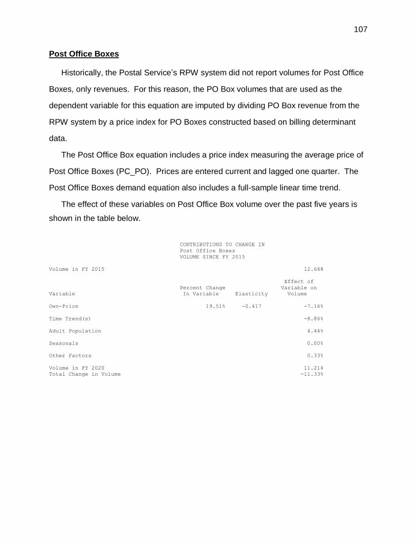
107

Post Office Boxes

Historically, the Postal Service’s RPW system did not report volumes for Post Office

Boxes, only revenues. For this reason, the PO Box volumes that are used as the

dependent variable for this equation are imputed by dividing PO Box revenue from the

RPW system by a price index for PO Boxes constructed based on billing determinant

data.

The Post Office Box equation includes a price index measuring the average price of

Post Office Boxes (PC_PO). Prices are entered current and lagged one quarter. The

Post Office Boxes demand equation also includes a full-sample linear time trend.

The effect of these variables on Post Office Box volume over the past five years is



Post Office Boxes



Effect of



Own-Price 19.51% -0.417 -7.16%



Seasonals 0.00%

Other Factors 0.33%



narrative explanation of econometric demand equations for

Documents