N91-24138RESULTS OF CORRELATIONS FOR TRANSITION LOCATION ON A

CLEAN-UP GLOVE INSTALLED ON AN F-14 AIRCRAFT AND DESIGNSTUDIES FOR A LAMINAR GLOVE FOR THE X-29 AIRCRAFT

ACCOUNTING FOR SPANWISE PRESSURE GRADIENT

S. H. Goradia

Vigyan Research IncorporatedHampton, Virginia

and

P. J. Bobbitt; H. L. Morgan; J. C. Ferris; and W. D. HarveyNASA Langley Research Center

Hampton, Virginia

SUNNARY

Results of correlative and design studies for transition location, laminar

and turbulent boundary-layer parameters, and wake drag for forward swept and

aft swept wings are presented in this paper. These studies were performed withthe use of newly developed, improved integral-type boundary-layer andtransition-prediction methods. Theoretical predictions were compared with

flight measurements at subsonic and transonic flow conditions for the variable

aft swept wing F-14 aircraft for which experimental pressure distributions,transition locations, and turbulent boundary-layer velocity profiles have been

measured. Flight data were available at three spanwise stations for severalvalues of sweep, freestream unit Reynolds number, Mach numbers, and lift

coefficients. Theory/experiment correlations indicate excellent agreement forboth transition location and turbulent boundary-layer parameters. The results

of parametric studies carried out during the design of a laminar glove for the

forward swept wing X-29 aircraft are also presemted. These studies includedthe effects of a spanwise pressure gradient on transition location and wake

drag for several values of freestream Reynolds numbers at a freestream Machnumber of 0.9.

INTRODUCTION

The rise in jet fuel prices during the last decade, and uncertainties ofthe fuel costs for the future have been the cause of continued worldwide

interest in improving military and commercial aircraft fuel efficiency.

Additionally, improvements in the range of military aircraft are additionalfactors for achieving aircraft fuel efficiency and drag reductions. The most

promising aerodynamic means of achieving significant gains in aircraft fuelefficiency is to design wings that provide extensive regions of laminar flow(refs. I and 2). Laminarization of the boundary layer on the surface of an

167

https://ntrs.nasa.gov/search.jsp?R=19910014825 2020-04-15T11:47:40+00:00Z

aircraft wing can be accomplished by the use of concepts such as Natural

Laminar Flow (NLF), Laminar Flow Control (LFC), and a combination of NLF and

LFC which is referred to as Hybrid Laminar Flow Control (HLFC).

Extensive regions of laminar flow can be maintained on a wing surface with

the NLF concept by suitably tailoring the spanwise and chordwise pressure

gradients to limit the amplification of disturbances that trigger the

transition of the laminar boundary layer to a turbulent one. Flight tests at

the Dryden Flight Research Facility on a variable sweep TACT F-111 Fighter

aircraft (ref. 3) with an NLF wing glove have demonstrated that natural laminar

flow can be maintained over significant areas at transonic speeds. Recent

flight tests of a laminar clean-up glove (a thin, smooth fiberglass coating) on

an F-14 aircraft with a variable-sweep wing (ref. 4), equipped with

instrumentation for the accurate determination of transition, also revealed

similar phenomena. Correlative studies were performed during the present study

for the F-14 aircraft laminar wing, clean-up glove using the methods of

references 5 and 6 extended to account for spanwise pressure gradient

effects. Results of these studies are presented in this paper in the form of

theory/experiment correlations for transition location and turbulent boundary-

layer parameters. In addition, comparisons of the hot-film experimental data

on the F-14 aircraft's wing glove with theoretical predictions are described.

The design of either forward- or aft-swept laminar flow wings at subsonic,

transonic, or supersonic speeds, using NLF, HLFC, or LFC concepts requires the

use of reliable theoretical computational methods. A number of finite-

difference boundary-layer methods, stability methods, and full Navier-Stokes

equation solvers are available; however, these methods are not well suited for

the large number of calculations required for parametric wing design and

optimization studies. Several new theoretical integral-boundary-layer methods

(references 5, 6, 7, and 8) have small computer execution times and are very

simple to use. These codes have the capability of predicting the laminar,transitional, and separating turbulent boundary layers for applications at

subsonic, transonic, and supersonic Mach numbers.

The design studies reported in this paper involve the design of an NLF

glove for the forward swept X-29 wing. The methods of references 5, 6, 7, and

8 have been modified for the present theoretical investigations to allow

consideration of the effects of spanwise pressure gradient. Results are

presented utilizing these modified codes for various spanwise pressure

gradients and a prescribed streamwise pressure distribution to determine the

extent of laminar flow on the corresponding X-29 wing glove. The wing

sections' upper-surface geometrical changes required to obtain the prescribed

pressure distribution are also given. Furthermore, the present design, _ =.... optimization Studies show qualitatively the procedure for Optim_ values of

=spanwise gradients so as to minimize the wake drag with due Consideration of

the effect of imbedded shocks on the boundary layer. Finally a comparison of

the extent of laminar flow on "equivalent" forward-swept and aft-swept wing

configurations is made.

168

NOMENCLATURE

AR

ASW

C

CDi

CDwake

Cp

CPsoni c

ACP1 or ACPc

C1 i

C1r

C2 i

C2 r

e

FSW

H

I,M,NK, _

L oE°

M

N.F.

P

Pr

aspect ratio

aft swept wing

chord 2

CLinduced drag coefficient -

wake drag coefficient

pressure coefficient or specific heat of air at constant

pressure

pressure coefficient corresponding to local Mach numberof 1.0

defined in figure 18

indicator of either growth or decay of disturbance for Ucomponent of velocity in transformed plane

downstream rate of propagation of disturbance for U

component of velocity in transformed plane

indicator of either growth or decay of disturbance for W

component of velocity in transformed plane

spanwise rate of propagation of disturbance of W component

of velocity in the transformed plane

wing efficiency factor for induced drag

forward swept wing

form factor = 6___e

groups of dimensionless parameters in transformed planes

presenting the effects of suction, pressure gradient andcurvature of velocity profiles. Each symbol defined intext.

leading edge

Mach number (used only with subscripts)

transition or instability due to normal flow

static pressure

Prandtl number

169

q

Qxor

Qz

R

RT,n

Rinst

Rtran

S,_,Z

S,F,

T

T.E.

U,V,W

U,V,W

dynamic head

dimensionless parameter representing effects of suction and

pressure gradient on the shape of velocity profile in

transformed plane

Qx - a2T's dUe VsaT's ; Qz a2,z dWe VsaT,zvo _X- + vo = vo dZ vo

freestream Reynolds number based on chord -

We/6T, n

Vm

value of RT, n at neutral point

value of RT, n at transition

U cGO

vO0

curvilinear coordinates in physical plane; s is normal to

local sweep lines on wing surface, { normal to wing

surface, and z normal to s-{ plane in spanwise direction

transition or instability due to spanwise flow

temperature, OR

trailing edge

velocity components in physical planes in s, { and z

directions, respectively

velocity components •in transformed planes in X, Y, and Z

directions, respectively

wing section coordinates in streamwise direction

Stewartson's transformed coordinates

s ae Pe ae Pe { T

X = f _ a-_F-ds;o o Y - ao Po _ T_d_

_2

@l(y)

disturbance stream function for transformed plane X-Y

disturbance stream function for transformed plane Z-Y

disturbance amplitude function for X direction in

transformed plane

170

@2(y)

_2

disturbance amplitude function for Z direction intransformed plane

2_/(wavelength of disturbance in transformed plane in X-direction)

2./(wavelength of disturbance in transformed plane in Z-direction)

dynamic viscosity

proportionality constant for viscosity-temperaturerelationship

kinematic viscosity

momentum thickness in physical s, { plane for 2-D or 3-D

normal direction c) = I pu (i - uU---)d_o PeUe e

momentum thickness in transformed X, Y plane for 2-D or 3-D

U (1 _ U)dyO e

eT,Z

8p,s

momentum thickness in transformed Z, Y plane

e e

6p,spu (1 u

I Pe Ue - _-] d_o e

ep,z

6p,z

I pw (I w- _-)d{o PeWe e

ep,n

6_ W

f p,n pu (1 _-)d_o PeUe e

6p, n greater of 6p, s or 6p, z

171

6

6

boundary-layer thickness in physical plane

: f6 (I pu )d{o PeUe

6T boundary-layer thickness in transformed plane

J

displacement thickness in transformed X, Y plane for2-D or 3-D

u )dYo e

displacement thickness thickness in transformed Z, Y plane

= f® (I- _-_)dYo e

Te**T,X T,n _1 - ) T-- dYo e

6T,Z

Ai :i T

Y

Te

0 e

_T,n greater of 6T, X or 6T, Z

local sweep angle in degree

ratio of specific heats for air

: 2y/b

Subscripts

o

ET 1 Z

" e,s

stagnation condition

edge of boundary layer in s-direction

e,z

aw

edge of boundary layer in z-direction

adiabatic wall condition

m

_ ._N

mean or average value over boundary-layer thickness

normal section

P physical plane

172

p,s

p,z

p,n

S

T

T,X

T,Z

W

X

Z

L.E.

T.E.

6

o

OO

S

physical plane in s-direction

physical plane in z-direction

either p,s or p,z

direction normal to local sweep lines

transformed plane

transformed plane X-direction

transformed plane in Z-direction

conditions at wall

transformed X-di rection

transformed Z-di rection

conditions at leading edge

conditions at trailing edge

parameter based on boundary-layer thickness

parameter based on momentum thickness

freestream value

measured in streamwise direction

In addition to the above list of symbols and subscripts, symbols and

subscripts are also defined at appropriate places in the text.

DESCRIPTION OF THEORY

A description of the theory for the integral methods used to compute the

laminar boundary layer, transition, and the turbulent boundary layer on a swept

wing is given in references 5, 7, and 8. These theoretical methods were

developed for infinite-span swept wings at subsonic and transonic speeds, and

for two-dimensional airfoils and bodies of revolution at supersonic speeds.

However, they did not include the effects of spanwise pressure gradient and the

resulting effects on the location of transition. The boundary-layer "wash-out"

phenomena are present on finite aft swept wing configurations with a given

taper and twist, whereas the boundary-layer "wash-in" phenomena are present on

configurations with forward sweep. The above theoretical methods of references

173

5, 6, and 7 have been extended in the present paper to account for the effects

of spanwise pressure gradients on laminar boundary-layer transition. At thepresent time, the effects of suction on the extended method are not considered.

The theoretical programs, which have been developed and used in the

present theoretical investigations of the wing glove of the F-14 aircraft andfor the parametric design studies of the forward swept wing of the X-29

aircraft with a laminar flow glove, are classified and enumerated as follows:

. Potential/Viscous Design and Analysis

a. Perturbation Method of Characteristics for inverse design at transonicMach numbers.

b. Bauer-Garabedian-Korn Program for transonic analysis.

c. NASA'Lockheed Multi-component Airfoil Program for subsonic analysis.

J

2. Boundary-Layer Analysis

a. integral Compressible Laminar Boundary-Layer Method with arbitrarychordwise pressure distribution and spanwise pressure gradient, sweepand suction at subsonic through high supersonic speeds.

b. Short bubble and reattachment criteria.

c. Instability and transition prediction due to leading-edge-normal andspanwise flow including the effects of spanwise pressure gradient.

d. Separating turbulent boundary-layer method from subsonic to transonicspeeds.

3. Method for computing CDwak e for an infinitely swept wing from subsonic

through supersonic speeds.

4. Modified strip method to account for the effects of taper, sweep, and twiston wing-section characteristics.

The theoretical development o--f the laminar boundary-layer method for an

infinitely swept wing will be briefly described. In addition, the methodology

for determining the effects of spanwisepressure gradients on laminar boundary-layer growth and on transition location will be outlined.

Governi ng Equations

The usual governing equations for a compressible hydrodynamic boundary

layer on an infinitely swept wing for the coordinate axis system shown infigure i are the continuity, streamwise momentum in s-direction, and momentum

174

in the { and z directions. The coordinate axis of figure 1 is chosen for the

purpose of facilitating the application of the present theory to the design of

the wing sections for an arbitrary wing planform. Moreover, the determination

of the effect of the spanwise pressure gradient on the extent of laminar flow

on swept wings by the present methods is greatly facilitated by the use of the

coordinate axis system selected. Thus,

@(pu) + @(pv) _ 0 Continuity (la)as @_

Bu @u _ @P + @ @u (s-direction (Ib)pu _-_ + pv @_ @s @--_-{_ -@_) + momentum)

@P - 0 (Normal Momentum) (lc)

Bw @w + B (u Bw

(z-direction

spanwise

momentum]

(Id)

The above equations (1) contain the terms consisting of variable physical

properties, such as density p and dynamic viscosity u. Variations of these

properties across the boundary layer as well as along the flow direction are

not negligible for laminar boundary-layer flow at transonic speeds and are

accounted for. At supersonic speeds, variations in the physical properties are

very large which means that there is a strong coupling between solutions of the

hydrodynamic and thermal boundary-layer equations.

In order to simplify the governing equations (1) for solution by integral

techniques while maintaining realistic computational results for the

hydrodynamic and thermal boundary layers, the use of the following Stewartson's

transformation is made:

s ae Pe

ae Pe { T

aoOoIO

175

where a is the proportionally constant for the viscosity-temperature

relationship, namely

u T- O&

I_ 11/2 TO + 198"6= aw

T-'o-/ Taw + 198.6

(3a)

(3b)

Taw

T0 C1 + TY-1 M2e)

(3c)

Furthermore, if it is assumed that the viscous flow on the wing can be

divided into a finite number of suitably oriented strips on its surface, and

that each infinitesimal control volume of the strip is a portion of an

infinite-span swept wing, then the governing equations of motion in the

physicai_:and transformed planes can 6e further si'mp!ified. =The: transformed

boundary-layer eqUations using Stewartson's transformations, for infinite-span

swept wing conditions, which can be derived from equations (1) with adiabatic

wail temPerature, are written as,

au av+ _ = 0 (4a)

aU aU dUe a2U

v = UedT +(4b)

@W @W @2W

U T_+ v_= Vo ay2 •(4c)

The relationships between the velocities within the boundary layer and the

pressure gradients in the physical and transformed planes can be written

a o

V :-- v (for adiabatic wall); W = wBe

- m ao dT (1 +TY-I M_4eJ

(Pr _ 1) as

aoU = _-- u;

e

due 1

(5a)

(5b)

i

i

!i

|

i

|

176

= ,

while the applicable boundary conditions in the transformed planes are given

by,

@ Y = 0+ U = W = 0,

a

- a° VwV = Vse

(6a)

@ Y = aT,X U = Ue = aoMe, aU _ a2U 0 (6b)+ ay ay_ =

and

@ Y = 6T, Z ÷ W = We = we ,

aw a2w= =

y--Z o (6c)

The compatibility conditions at the surface of the wing in the transformed

planes can be written as,

- V r@U_ = dUe ra2U_

@ Y = 0 + s_-jw Ue dT + VO_ay2Jw- (7a)

fa2u_ ra3u_

@ Y = o + - Vst@Y--Y-_)w = v°_@Y-Y-3-)w (7b)

and in the absence of suction for flows with spanwise pressure gradients,

1 aPp az ae a2W J

Y=0 - ao v° --BY2 Y=0(7c)

The integral equations in the transformed planes in the leading-edge normal

direction X and in the spanwise direction Z can be derived by making use of

equations (4), boundary conditions (6), and wall compatibility conditions

equations (7), and by use of Leibnitz's rule.

Momentum Integral Equation in X-Direction, Infinite Swept Win 9 Conditions

U d _ Sex- + 2) - ]e dX-( ) = 2 [L K(HT, s(8)

177

Momentum Integral Equation in Z-Direction, Infinite Swept Wing Conditions

aT'n U (I - _-)dY] = VoC-_)y= 0d [U Wel li-e 0 e e

- VsWe (9)

where 6T,n is greater of _T,Z or _T,X"

The symbols L, K, and SQ appearing in the above equation (8) are definedin equation (20) for transformed X and Z coordinates.

The velocity profile assumptions for the flow in the X- and Z-directions

in the transformed planes are given by the following equations,

where

uU _ Alnx + A2n_ + A3nx3 + A4nx4e

YnX -

aT,X

(lOa)

and

A1 = 2 + QX/6;

A3 = -2 - A2;

A2 = -O.5Q X;

A4 = 3 - AI

=

(10b )

(ii)W - 2n Z 2n_ + 4W - nze

Y

where, nZ - 6T 'Z '

The numerical solutions of equations (8) and (9) are performed by the

Euler method with _epeatedwiterations. These solutions give the shape of

velocity profiles _ and _-- in the transformed planes under the assumption ofe e

infinite-span swept-wing conditions.

178

EFFECTS OF BOUNDARY-LAYER MASH-IN/WASH-OUT DUE TO SPANWISE

PRESSURE GRADIENTS ON TI_SITION ON FINITE, SWEPT,

TAPERED, AND 1WISTED WING

The results of theory/experiment correlations for several wings using both

wind tunnel and flight-test data have indicated that for sweeps greater than

approximately 25°, and freestream Reynolds numbers greater than 20 million

transition is triggered by spanwise flow in the z direction. Thus, for the

purpose of designing laminar-flow wings and gloves at transonic and supersonic

speeds at Reynolds numbers and sweeps of practical interest, it is necessary to

consider the effects of boundary-layer wash-in/wash-out due to spanwise

pressure gradients. This is especially important for wings of supersonic

aircraft where the sweep of the leading edge is usually in excess of 450 . In

order to account for the effects of boundary-layer wash-in/wash-out on finite

swept wings the approach shown schematically in figure 2 is used. This figure

shows the infinitesimal control volume composed of surfaces of a trapezoid.

The coordinate system is the orthogonal s, { and z axes where the s

coordinate is normal to the local sweep line, z-coordinate is normal to s in

the plane of wing, and the {-coordinate is normal to the s-z plane. AIB 1

and CID 1 are constant s/c lines where c is the local chord in s-direction

and AID 1 and BlC 1 are parallel to s-direction.

The momentum theorem is applied in the z-direction, which states that the

algebraic sum of the forces acting on the control volume ABCD - AIBICID 1 in

the z-direction is equal to the rate of change of momentum in control volume

plus the net flux of momentum in the z-direction across the control surfaces of

the control volume. For steady mean flow conditions an equation can be derived

for the boundary-layer wash-in/wash-out due to spanwise pressure gradient

W

effects on velocity profile _- in the z-direction. This equation in thee

physical coordinate system for transformed boundary-layer quantities can be

written as: 2

1 dCz__p- a We M_,z_- (0T,z)N = { T_ [(°T,Z)o U---2 (1 + 0.2 )0.5]

CO

We Ue M2 )0.5 [ 1+ U U (1 + 0.2 e,s M

® CO e,s

d Me,sds (6T,X) o (0.7 + 0.00833 Ax)

dAX

+ (0.7 + 0.00833 ^X ) -_s (aT,X)o + 0"00833(aT,X)o _ ]

Pw We 1 1

---_o " _o'U--CO " U--CO(OT,z) o, O. 235

(1 + 0.2 Me,s2)-3

(1 + 0.171 Me,s2) }

• (1 + 0.2 M2)

e,z

-342

(1 + 0.2 MCO2)2"5/ (8.547 + 0.711 le,z) (12)

179

where

(eT,Z) N =Transformed momentum thickness in Z-direction

which is modified by the boundary-layer wash-in/

wash-out phenomena due to spanwise pressure

gradients on finite-swept and tapered wing.

(eT,z)oTransformed momentum thickness in Z-direction for

infinitely swept wing assumption conditions.

dU

1 e _Ax = (6 ,X)o Vo dX

Dimensionless pressure gradient parameter in

X-direction in transFormed-plane for infinite-span,

swept-wing assumption conditions.

(6T,X) o =Transformed boundary-layer thickness in X-direction

for infinite-span swept-wing assumption condition.

_w _ " To + 198.6 due to Sutherland

_o Taw + 198.6 theory of viscosity.

The following approach is used for the purpose of calculating (aT Z)g andthe velocity profiles in the transformed plane in the spanwise directi6n in

order to account for the boundary-layer wash-in or wash-out phenomena.

Define the quantities,

and,

= (62T,Z)N ( 1 dWeAZN vo d Z )=

dW

= (e2T,Z)N ( 1 e)BZN vo dZ

(13)

where:

(_T.Z)N = Transformed boundary-layer thickness in Z direction which is

modified by the boundary-layerwash-in/wash-out phenoena due

to spanwise pressure gradients on finite-swept and tapered

wing.

If a fourth order velocity profile is assumed in the spanwise Z direction

in the transformed plane, then the relation between AZN and BzN can be derivedas the fol lowing polynominal :

180

^ZN = P1 + P2BZN + P3B2ZN +

3 4 5

P4BZN + PSBZN + P6BZN

where,

P1 = 0.032015

P2 = 73.156

P3 = 10.587

P4 = -129.6

P5 = 4669.6

P6 = 43865.0

thus, (_T,Z)N can be written as, (_T,Z)N = (BT,Z)N / (BZN /^ZN )1/2

The velocity profile _ in the transformed plane can therefore be calculatede

from the following assumed fourth order polynomial given by:

W + B3n_W - BlnZ + B2n2ze

4+ B4n Z

where,A.

Y __ 1nz = T_ N and B1 = 2 +__; B2 = - _ AZN

B3 = -2 - B2; B4 = 3 - B1

THERMAL BOUNDARY-LAYER SOLUTION

Temperature variations within the boundary layer at subsonic speeds are

small, hence the effects of temperature variations within the boundary layer on

instability and transition at subsonic speeds are neglected. However, at high

transonic and supersonic speeds, the heat generated by friction and adiabatic

compression is quite significant. These phenomena give rise to large

temperature variations across the boundary layer, and it has been found from

computational experiments that these large temperature variations affect the

following equations for computing temperature profiles; they can be derived

using the procedures described earlier.

]8]

U2

T-T Tw - TW-TeyTaw (_--)-e J__e (_e)2

eY=6T, X = 6T, x

(14a)

_ 2

T - Tw Tw Taw (_--) - _Pr_-gWeTo C-_-)2Up ,14b)T T e e

eY=6T, Z eY=6T, Z

For determining the temperature profile at a given location on the wing

use is made of either equations (14a) or (14b) depending upon whether 6T,X is

larger than aT,Z or vice versa. The velocity profiles _- or W__W in thee e

transformed planes in X or Z direction, which are required in equations (14a) or

(14b), are dependent on local pressure gradients in the leading edge normal-s

or spanwise-z directions due to use of equations (9) or (11), respectively.

Thus, the effect of pressure gradient and suction is implicitly accounted for

in the determination of temperature profiles by the present method.

Criteria for Determining Locations of Neutral Instabilities

for Velocity Profiles in s and z Directions

The Orr-Sommerfeld equations in transformed planes for X and Z

directions can be written as follows: For the transformed coordinate in the X-

directi on,

( sl(U - C1)(¢]' - a1¢1, - Uyy¢ 1 :IROT, X

and for the transformed coordinate in the Z-direction,

2 ,, 4, _ i [¢_,,, _ 2_2@2 + a2@2 ]

(W - C2)(@ _ - _ @2 ) - Wyy@ 2 _2RBT, X

(16)

The disturbance stream functions for the transformed X and Z directions

are assumed, as for the physical plane, as the following types:

im1(X-Clt)

_ = @l(y)e ÷ X-direction(17a)

i_2(Z-C2t)

_ = @2(y)e ÷ Z-direction(17b)

182

|

where,

@I(Y) and @2(Y)disturbance amplitude function

for X and Z direction, respectively

in transformed planes

_1 and m2 = 2,/(disturbance wavelength in transformedplanes in X- and Z-direction, respectively)

X = transformed coordinate for s-direction

Z = transformed coordinate for z-direction

C1 = C1 + iClir

C2 = C2 + iC2.r l

complex in general

C1, or C2. = 01 I

>0

<0

corresponds to neutral instability

corresponds to amplification of disturbance

corresponds to decay of disturbance

The generalized solution between the dimensionless pressure gradient

parameters and "equivalent" Reynolds number based on momentum thickness for the

neutral stability of laminar boundary layers in either s or z direction is

shown in figure 3. The curve shown in this figure is derived from solutions of

the Orr-Sommerfeld equations, equations (15) and (16), in the transformed X-Y

plane or Z-Y plane for appropriate fourth-order polynomial velocity profiles.

The effects of pressure gradient in the s-direction or z-direction, local Mach

number, temperature profile, and suction have been accounted for in the

derivation of this curve. The abscissa of figure 3 is given as the zero

suction ( SO = O) version of

Op,sdMe, s 1

1 1 ds 1 Se

ao _- or • [I - LX ] (18)

dz ( i + 0.2 'z2 ) (M + S0 OrLz)

183

where

Vm -

1 n

_n _0 _d{

6n = greater of _p,s or 6p, z

(M esIe,z

(19)

In equation (19), the term (T) or CT-L-)T for temperature profile aree,s e,z

substituted from equations (14a) or (14b).

It should be noted that because of the choice Of the coordinate axis

systems shown in figures 1 and 2, it is possible to use the same criteria shown

in figure 3 for determining the neutral stability point for disturbances in

both the normal and spanwise directions,

Boundary-Layer Transi ti on Cri teri a

The Criteria used in the present method for determining the transition

locat#6n=_e i_o the amplifica{ionof disturbances eithe{ in the normal or

spanwise directions are shown in figure 4. The parametric curves of figure 4

are valid for arbitrary specified pressure gradients- both in the normal as

well as spanwise directions. The independentand dependent variables shown in

this f-i-gu_ contai_n groups of several hydrodynamic and thermal boundary-layer

P_ara'met_ w_are sign_-f_c-ant_ur_ng _tlie t-r_s_0-n_process, fn derivin_the curve for low values of freestreamturbulenCe (iess-i_h-an--.()5 percent), the

use of experimental data obtained in flight .Or Iow-turbulencewind tunnels ismade and this info{mat_on is put in the transformed planes Thee dimensioniess

parameters shown !n_figure 4 have been derived from di_nsional anaiyses and bymaking us e of the laws of dynamic similarity. These physical dimensionlessparameters consist of the following:

2 2C)T,X dUe , °T,Z dWe

KX - _o dx KZ: _o dZ

t

eT,X aULX - U (_]Y:0 ;

e

@T,Z aW

LZ - We CaY-)Y:0

184

o2 2..

_ F,X (_-u]MX Ue _ Y=O

_ °T,XVs OT,ZVs

Sox v o ; Soz - Vo

** W 6"*Ue6n e n

RN - ; RN -x Vm z Vm

® T _ T

_ " (S** (i We): Ci - x : Inx ' nz o

Y Y- ; nZ -

nx aT,X 6T,Z

(___ __ pressure_ (20)T _ Temperature W , Pr, ML, gradientJTe Profile = F , We

In deriving the curves for several higher values of freestream turbulence

greater than 0.05% shown in figure 4, use has been made of information

presented in figure 5 for a zero pressure gradient and for values of Mach

number from low subsonic to high supersonic (up to M® = 4.0). It has been

hypothesized in constructing the curves of figure 4 for values of freestream

turbulence greater than 0.05 percent, that the effect of pressure gradient for

freestream turbulence greater than 0.05 is similar to low values of freestream

turbulence of 0.05. Curves for freestream turbulence higher than 0.05 percent,

shown in figure 4, have been constructed by making use of information in figure

5 and using the above hypothesis.

It needs to be pointed out here that the curves of figure 5 can also be

used for other types of disturbances, e.g., noise generated due to the

turbulent boundary layer on the walls of the test section of supersonic wind

tunnels. This objective can be accomplished after the application of

appropriate calibration procedures.

Turbulent Boundary Layer

It has been known from experimental data on sections of NLF wing s that if

turbulent separation is present upstream of x/c _ 0.95, then the design

pressure distribution necessary to maintain laminar flow is degraded.

Additionally, the wake drag will be quite high due to presence of the separated

flow region. In the present paper turbulent boundary-layer separation is

185

accounted for by the method developed in reference 8. This turbulent boundary-layer method has already been successfully applied in the design of NLF and

HLFC wing sections and for the prediction of wake drag.

To compute the turbulent boundary layer from the location of transition atvarious spanwise stations to the wing trailing edge, the method of reference 8

was modified to account for effect of spanwise flow assuming infinite swept

wing conditions. The important objectives for the computations of theturbulent boundary layer are: (I) to see if turbulent separation is presentdownstream of the transition location, and (2) to determine the turbulent

boundary-layer quantities at the wing trailing edge.

The theoretical method of reference 8 has been developed by analyzing themean and fluctuating components of velocity profile data obtained by the use of

a laser velocimeter for several airfoils with trailing-edge seperation. Theseexperimental data indicated that as the turbulent boundary layer approached the

separation location, the fluctuating velocity components become of the sameorder of magnitude as the mean velocity components within the turbulent

boundary layer. This observation suggested the retention of the fluctuating-velocity components in the governing equations of motions as was done inreference 8. This method has been found to be extremely reliable in predicting

turbulent boundary-layer quantities, including separation, on wing sectionswith thickness ratios in the range of 0.09 < t/c < 0.22 and Reynolds numbersfrom 2 to 30 million.

Computations of CDwak e for Wing Sections

The derivation of the expression for CDwake for an infinitely swept wing

is given in Appendix A. This expression, which is valid from subsonic tosupersonic speeds, is given as

CDwake

Pe uU__.ee)p= 2 [( (p-_)T E ( COS2AT Ec Ouu)T.E. . . ® . .

W

Pe eT+ (Ouw)T.E. (p-_)T.E. (w® .E.) sin2AT.E.]

where the exponent p is given by

p = [HT.E. + 5 + (y-l)M_ee]/2.0 (21)

The CDwake for a finite tapered swept wing can be computed from equation

(21) and by making use of modified strip theory.

186

APPLICATIONSOFTHEPRESENT THEORETICAL METHODS

The theoretical methods described in previous sections are utilized to

perform two tasks in the following section, namely:

(i) The predition of transition location and turbulent boundary-layer

parameters on the "clean-up" glove of the F-14 aircraft and

correlation with experimental data.

(ii) Performing parametric studies for the design of a laminar glove for

the forward swept wing of X-29 aircraft.

Correlation with Experimental Data on the Glove of F-14 Aircraft

The planform and instrumentation for the gloved F-14 wing with 20° sweep

is shown in figure 6. With the "clean-up" glove installed, the sweep of the

wing leading edge was varied from AL.E. = 200 to AL.E. = 35°, and the flaps and

slats were locked in the up position. As shown in figure 6, the three rows of

surface pressure orifices are located at spanwise stations n = 0.515, 0.67, and

0.83, respectively, and were oriented in a direction parallel to freestream for= 200 . In order to avoid interference

the wing leading edge sweep AL.E.between hot-film gauges, they were placed at an angle of 300 to rows of surface

pressure orifices as shown in this figure. The boundary-layer rakes were

installed at two spanwise locations at x/c = 0.55 in order to measure the

turbulent boundary-layer velocity profiles. Transition and turbulent boundary-

layer data were obtained for freestream Mach numbers from 0.6 to 0.8, wiRg

leadiRg edge sweeps from 20° to 350 , and a Reynolds number range of 8x10 v to25x10 v. Pressure distributions for the aforementioned three spanwise

locations were also measured for these Mach numbers and sweeps. These pressure

distributions constituted the boundary conditions for computing both the laminar

and turbulent boundary layers and the transition location on the F-14 glove.

Figure 7(a) shows the pressure distributions on the upper surface of the

glove at three spanwise locations and hot film traces at station 2

(n = 0.67) for the wing leading edge sweep of 200 , M = 0.7 and a freestream

Reynolds number based on chord of 13 million. In adJition to using the

pressure distributions as boundary conditions, they are used to evaluate the

effect of spanwise pressure gradient on the development of the laminar

boundary layer and transition location at station 2. Since the experimental

pressure data only extended back to x/c = 0.6 theoretically computed pressures

distributions were used from x/c = 0.6 to trailing edge in order to compute

the growth of turbulent boundary layers from the transition location to the

trailing edge. Figure 7(b) shows the computed results for chordwise

transition and instability location due to normal flow (N.F.) and spanwise

flow (S.F.) phenomena. The results are plotted in this figure as x/c of

instability and transition versus freestream Reynolds number. These results

indicate that at a Reynolds number of 13 million, the computed transition

187

location is due to N.F. phenomenaand occurs at x/c : 0.33. The hot filmtrace shownin figure 7(a) shows that the experimental transition location atstation 2 is between0.3 < x/c < O. 4. Thus, good agreement is obtainedbetween the theoretically computedtransition location and the hot-film-measured transition location. Figure 7(c) shows the results of computationsfor displacement thickness, 6"/c, momentumthickness, o/c, and form factor H,plotted against x/c for station 2. Freestream Machnumber, Reynolds number,and leading edge sweepfor the results shownin figure 7(c) are the sameasfor figures 7(a) and 7(b). Experimental data for 6"/c, o/c, and H at x/c =0.55 for station 2 in the turbulent boundary-layer region are also plotted infigure 7(c). These results indicate that present theoretical computations forthe turbulent boundary-layer parameters agree quite well with theexperimentally measuredquantities. Furthermore, these results indicate thatthe location of transition predicted by the present theory must be in closeagreement with experimentally determined transition. It is also interestingto notice from figure 7(c) that the slope of o/c versus x/c in the laminarflow region is smaller than that in the turbulent region. This large slope ofo/c versus x/c in the turbulent boundary-layer region will lead, of course, tolarge values of e/c at the wing trailing edge. The wake drag coefficient,

CDwake, is directly proportional to the momentumthickness, o/c, at the

trailing edge.

Figures 8(a) and 8(b) show plots o{ experimental pressure distributionsand hot film traces for M = 0.801, a leading edge sweep of 20° and freestream

Reynolds numbers of 11 miTlion and 23 miiT_on, respectively. As can be seen

from the comparison of pressure distributions in figures 8(a) and 8(b), thereis not any noticeable difference in pressure distributions between Reynolds

numbers of Ii and 23 million, and hence, the same pressure distributions atthree spanwise stations were used for computations of transition and

instability results for the range of Reynolds number shown in figure 8(c).

These pressure distributions indicate that the shock strength is high, and forthis reason, there seems to be some discrepancy in computed and measuredturbulent boundary-layer parameters at x/c : 0.55, as shown in figure 8(e),

even though the transition location is predicted quite accurately. The presentshock boundary-layer model is being refined in order to provide better initial

conditions for turbulent boundary-layer computations downstream of a strongshock.

AS seen from figure 8(c), the computed transition location for a

freestream Reynolds number of 11 milli_]s at x/c _._ and caused by N.F. :phenomena, however, at a frees treanl Reynolds number of 23 million the computed

results indicate that transition is _au_d by S.F. phenomena and occurs atx/c = 0.41. Experimental data from the hot film sensor shown in f_gure 8(a)indicate that at a Reynolds number of II million, transition occurs at

x/c _ 0.5. Hot film traces at a Reynolds number of 23 million, which are

shown in figure 8(b), indicate that transition is occurring, for thisfreestream condition, at x/c _ 0.4. Thus, as seen from comparisons of

188

computed results, shownin figure 8(c), with hot film traces of figures 8(a)and 8(b), the present theory reliably predicts both the location of transitionas well as its mode, i.e., due to N.F. or S.F. phenomena. Figure 8(d) shows a

plot of computedCDwake as a function of freestream Reynolds number. As seen

from this figure, CDwake decreases as the freestream Reynolds number increases

from 8 to 20 million and above the Reynolds numberof 20 million CDwake

increase with Reynolds number. The Reynolds numberof 20 million, where the

computedCDwake becomesminimum, corresponds to the initial triggering of

transition due to spanwise flow. This is an important phenomenaand one thatcan be used to advantage as seen in the design of a proposed laminar glove forX-29 aircraft discussed subsequently in this paper. Finally, figure 8(e)shows the plots of computedvalues of 6"/c, O/c and H versus x/c for aReynolds numberof 12.4x106.

Figure 9(a) shows the experimental pressure distributions and hot filmtraces for a wing-glove leading-edge sweepof 250, a freestream Machnumberof0.706 and a Reynolds numberof 11 million. By using the experimental pressuredistributions as boundary conditions (see figure 9(a)), the transition andinstability locations are computedand the results are shownplotted in figure9(b) as a function of freestream Reynolds number. Experimental data fortransition obtained from hot film traces, shownin figure 9(a), indicate thattransition for a wing glove leading edge sweepof 25.30, Reynolds numberof 11million, and N = 0.706 takes place for 0.4 < x/c ( 0.5. Theoretical results

mm

for these same conditions shown in figure 9(b) also show that transition

should occur at an x/c between 0.4 to 0.5.

Now, it is generally believed that if the freestream Mach number is kept

constant, that increasing wing sweep reduces the extent of laminar flow.

However, experimental data and calculations for the wing-glove leading-edge

sweep of 200 and M = 0.7, (figures 7(a) and 7(b)) when compared to results

for a sweep of 25°. figures 9(a) and 9(b), show that transition is located

closer to the leading edge for the lower sweep. Furthermore, comparison of

the calculated results of figure 9(b) with those of figure 7(b) indicates the

same phenomena. This is an unusual result and shows the ability of the

present methods to optimize wing section geometries and planforms for

extensive laminar flow regions at specified freestream conditions.

Figure 9(c) shows the results of theoretical computations for the laminar

and turbulent boundary-layer parameters _*/c, O/c and H plotted versus x/c for

a leading-edge sweep of 250 , N of 0.704 and a Reynolds number of

approximately 11 million. For®this case, strong shocks are not present at any

spanwise station, as can be seen from figure 9(a). The computed boundary-

layer parameters agree quite well in the turbulent boundary-layer region at

x/c = 0.55. This agreement of computations with experiment in the turbulent

boundary-layer region is an indication that the computed transition location

189

is fairly close to the experimental transition location. Moreover, these

results indicate the reliability of the present theoretical turbulent

boundary-I ayer method.

Figure lO(a) shows the experimental pressure distributions and hot film

traces for a leading-edge sweep of 29.70 , M = 0.704, and a Reynolds number of

9.5 million. The corresponding experimental data for a Reynolds number of

19.2 million and leading edge sweep of 31.40 are shown in figure lO(b).

Figure 10(c) shows theoretical results for instability and transition

locations for a leading-edge sweep of 300 and M = 0.704. These results show

that for a Reynolds number of 9 million transition takes place at x/c = 0.34

and is caused by S.F. instability phenomena. Experimental data obtained by

hot-film sensors, shown in figure lO(a), for a Reynolds number of 9 million

indicate similar results, namely transition takes place at an x/c between 0.3

to 0.4. At a Reynolds number of 19.2 million (figure 10(c)), transition due

to S.F. takes place at x/c _ 0.175; experimental hot film trace data for the

same freestream conditions, shown in figure lO(b), also indicate that

transition occurs between x/c of 0.1 to 0.2.

Design and Parametric Studies for Laminar Glove of X-29 Aircraft

It has been Observed from theoretical studies and experimental data that

wing sweep have a pronounced effect on transition location when the freestream

Mach number and Reynolds number are held constant. It is also believed by

many, from a conceptual view point, that it is easier to achieve large

laminar-boundary-layer-flow regions on a forward swept wing (FSW) than on an

aft swept wing (ASW). This is so because for FSW the local values of sweep

are lower near the leading edge and the local sweep angle increases from the

leading edge to the trailing edge; whereas, for ASW, sweep angle is the

largest near the leading edge and decreases progressively toward the trailing

edge. Figure 11(a) shows schematically a comparison of planforms for

"equivalent" FSW and ASW. The word "equivalent" implies that for both FSW and

ASW, wing area, aspect ratio, taper ratio, and shock locations are

identical. Figure 11(b) shows the plots of local sweep angle versus x/c for

FSW and ASW of aspect ratio of 4 and taper ratio of 0.4. The planform and

variation of sweep angle with x/c shown in figures 11(a) and 11(b) are a rough

approximation of the X-29 aircraft wing. The point C in figure 11(b), which

is at the intersection of local sweep versus x/c curves for the "equivalent"

FSW and ASW_ indicates that the local sweep angles for these "equivalent"

wings become equal at x/c _ 0.5. Thus the possibilities of maintaining

laminar flow for x/c < 0.5 on an NLF glove for the FSW of X-29 aircraft are

much greater than they would be for an "equivalent" ASW with a laminar glove,

It is possible to realize an additional advantage from forward swept

wings and this stems from the lower shock-wave drag. If the NLF design

pressure distribution is such that the minimum C. on the upper surface occurs

aft of x/c : 0.5, then the local Mach number at _he shock location for FSW

190

will be lower than that ahead of the shock on an "equivalent" ASW for the same

value of the freestream Mach number. This is so because the local sweep angle

for FSW is higher than that for an equivalent ASW downstream of point C

(x/c % 0.5) as can be seen from figure 11(b). These phenomena would result in

lower shock wave drag for FSW for the NLF design glove of X-29 aircraft, and

moreover, the susceptibility of the NLF design for FSW to turbulent separation

is also diminished. This is because the initial turbulent boundary-layer

thickness at the shock location would be lower for the FSW than for the

equivalent ASW.

The above discussion suggests that better prospects exist for overall

lower total drag for an NLF concept with FSW than one with an equivalent

ASW. The superior drag peformance due to application of NLF (or HLFC)

concepts to a FSW arise due to the possibility of achieving larger chordwise

runs of laminar boundary-layer flow, lower shock wave drag, and less

susceptibility to turbulent separation drag.

Figure 12 shows the planform of the X-29 aircraft. The canard and wing

are in the same plane. The wing has a leading-edge sweep of approximately 29°

and the trailing-edge sweep is 45o. The chord of the first flap extends from

x/c = 0.75 to x/c = 0.9 and that of the second flap extends from x/c = 0.9 to

x/c = 1.0. The wing leading-edge break is at n = 0.25, and the tip of the

canard is at n = 0.49. Experimental pressure distributions on the canard

suggest that boundary-layer flow separation exists on the canard and the

possibility exist that the separated wake of the canard may prohibit the

achievement of laminar flow on the wing between the wing root and the midspan

location. The forward swept wing has associated with it the boundary-layer

wash-in phenomenon, and for this reason it is believed that a laminar glove

can be designed so as to obtain extensive laminar flow on the outboard wing

from n = 0.55 to n = 0.95.

Simple-sweep methods or modified simple-sweep methods are frequently used

in the design of airfoil sections for aft swept wings. Different forms of

modified simple-sweep methods are employed but they give essentially the same

results. The present modified simple sweep approach for ASW is illustrated in

figure 13. The geometry of the normal section is arrived at from the geometry

of the streamwise section by the following expression:

where,

(z/C)Normal section

(z/C)streamwise section

Cos AL

AL = local value of sweep

= ALE + (ATE - ALE) • (x/c)

191

The pressure distribution is computed for the normal section by airfoil

programs, such as, Bauer, Garabedian, and Korn program (ref. 9) or Lockheed-

NASA multi-Component airfoil program (ref. 10). The computations for the

normal section Mach number and lift coefficient are made using

M®N : M® • COSAeffectiv eS

where,

M = effective component of freesteram Mach number for normal section"N

M = streamwise freestream Mach number

S

and, A effective = A @ x/c = 0.25 for subsonic and transonic freestream

Mach numbers

and

where,

CLN = CLS /C°S2Aeffective

CLN = lift coefficient for normal section

CLs = lift coefficient for streamwise section

The thickness of the normal section for the aft wing section is thus

greater than that of the streamwise section by the factor of 1/CosA L. Thepressure distribution computed for this normal section (with

M®N M®sCOSAef f and = / Cos 2 f) is related to the pressure

distribution for the streamwise section by,

Cp = • COS2ALStreamwise CPNormal

The application of the above-mentioned modified sweep approach to the

computation of the pressure distribution for the forward swept wing of the X- =

29 at n = 0.7, M® = 0.91 and C. = 0.351 is shown in figure 14. It is

apparent from this figure that _he theoretical pressure distribution Computed _,

by the above-mentioned modified simpie sweep method for aft Swept wings does

not agree with the experimental data for the FSW of X-29 aircra_t_ .... I

Consequenti_a_h_ modified simple'sweep'approach wa_ developed for the !

computation of pressure distributiOnS for forward swept wings, in this

approach, the ordinates of the upper surface of the normal section are kept

192

the same as for the streamwise section but the thickness distribution for the

normal section is increased by the cosine of the local sweep angle and is

given by

(t/c) Local = (t/c) Local / CosA LNormal Streamwise

Streamwi se Secti on

The remaining steps for the computation of the streamwise pressure

distribution are the same as for the aft swept wing. Both procedures are

illustrated in figure 13. The results of computations of the streamwise

pressure distributions, using the new modified simple sweep method, for the X-

29 aircraft for n = 0.7, M = 0.91 and C. = 0.351 are shown in figure 14. AsLseen in this figure, the agreement between the theoretical upper surface

pressure distribution computed by the new modified simple sweep method and

experimental data is reasonably good. Hence, the parametric studies for the

design of the outboard laminar-glove sections are conducted using this

approach.

In order to enlarge the extent of laminar flow for the X-29 wing, by the

installation of a wing glove, it is first necessary to determine the extent of

laminar flow on the existing X-29 wing. Theoretical computations for

instability and transition locations on the existing X-29 wing at n = 0.7 are

plotted in figure 15(a) as a function of freestream Reynolds numberL

Experimental pressure distributions are used for boundary conditions in this

calculation. The computed wake drag coefficient for the existing wing section

at n = 0.7 is plotted as a function of freestream Reynolds number in figure

15(b). The results shown in figures 15(a) and 15(b) illustrate that the

extent of laminar flow on the existing X-29 wing is quite limited and,

consequently, the wake drag is high for Reynolds numbers in the range of 8 to

30 million.

A number of pressure distributions and corresponding glove geometries

have been theoretically investigated in the present studies, under the

assumption of infinite-span swept-wing conditions. It is necessary that the

glove geometry be compatible with original X-29 wing such that the glove wraps

the wing surface with continuous first and second derivatives, and that there

be a smooth merging of the glove with the original wing surface. From these

considerations, the glove with the geometrical shape designated as XTM2P3K,

and shown in figure 16 for spanwise station n = 0.7 was developed. The

geometry of the baseline X-29 for the spanwise station of n = 0.7 is also

shown in figure 16 for comparison purposes. Figure 17(a) shows the computed

streamwise pressure distribution for this glove at n = 0.7 for M = 0.905,

CLs = 0.435 and a leading-edge sweep of 300 • The computed pressure

distribution for CLs = 0.351 for the baseline section is also shown in figure

17(a) for comparison. It is important to note the shape of CPsonic in figure

193

17(a). For the forward swept tapered wing, the CPsonic line has an upward

slope, whereas for the "equivalent" ASW the CPsonic line will have a downward

slope. These phenomena suggest, for the specified freestream Mach number and

value of Cp just upstream of the shock, that the FSW will have a smaller value

of shock wave drag than the ASW.

The streamwise pressure distribution computed for the glove with a L.E.

sweep of 25o, and CLs = 0.43 is shown in figure 17(b); since the sweep is

lower, the design freestream Mach number was lowered to a value of 0.865 (as

compared to an M of 0.905 for sweep of 300). The reason that the Mach number

was lowered was To keep the leading-edge normal Mach numbers constant. The

theoretical transition characteristics for the X-29 glove for leading-edge

sweeps of 300 and 250 and zero spanwise pressure gradients are shown in figure

17(c). As seen from figure 17(c), the S.F. instability triggers the

transition at a Reynolds number of 12 million for a leading edge sweep of 300 ,

and at a Reynolds number of 15 million for a leading edge sweep of 250 •

Figure 17(d) shows a comparison of the wake drag characteristics for the

X-29 glove for leading edge sweeps of 300 and 250 . Also plotted in figure

17(d) is the wake drag of the baseline section for a leading-edge sweep of

300 . These comparisons indicate the following phenomena, first, the wake drag

of the glove is lower than the basic X-29 wing section by as much as 17 to 18

counts at a Reynolds number of 10.5 million, and second, when the leading-edge

sweep is reduced from 300 to 250 , the freestream Reynolds number at which

minimum is increased from 10.5 million to 16 million.CDwak e becomes

However, it may not be possible to reduce the wing glove leading-edge sweep to

250 because of stability and control considerations.

As stated previously in the theoretical section, the methods of

references 5, 6, and 7 have been extended in the present studies to take into

account the effects of boundary-layerwash-in/wash-out and spanwise pressure

gradients on the development of the laminar boundary layer as well as

instability and transition locations. Thus, it was possible to conduct

parametric studies on the effects of boundary-layer wash-in phenomena and

spanwise pressure gradients on the triggering of transition due to S.F.

phenomena. Proper use of spanwise gradients can delay transition to higher

Reynolds numbers and result in a wake drag reduction at the cruise Reynolds

number. Figures 18(a) and 18(b) show the two types of spanwise pressure

gradients which have been utilized to study the effect of spanwise pressure

gradients on transition. In figure 18(a), constant spanwise pressure

gradients are assumed on the upper surface from 0 < x/c < 0.6; computations

have been performed for spanwise gradients, aCp , of 0.05, 0.1 and 0.15. Forc

the linearly varying spanwise pressure gradients depicted in figure 18(b), the

spanwise pressure gradient is a maximum near the leading edge and it decreases

194

linearly to zero at x/c = 0.6. Computational results are presented for

ACPI values of 0.05, 0.I, and 0.15. Instabilities and transition

characteristics due to N.F. and S.F. and wake drag characteristics for thevarious spanwise pressure gradients shown in figures 18(a) and 18(b) have been

determined. A few representative results are shown in figures 19 and 20.Figure 19 shows the plots of N.F. and S.F. transition characteristics for a

constant spanwise pressure gradient corresponding to ACp : 0.15. Alsoc

plotted in figure 19 for comparison are the results for N.F. and S.F.

transition characteristics on the laminar-flow glove for a spanwise pressuregradient of zero. It can be seen from these results that the Reynolds number

at which S.F. triggers transition increases from 12 to 20 million as the

spanwise pressure gradient is changed from zero to ACp = 0.15 (see figurec

18(a)). Furthermore, notice the change in N.F. transition characteristics for

these two cases. Calculations indicate that turbulent separation does not

occur in either of the cases shown in figure 19.

Figure 20 shows the plots of versus freestream Reynolds number forCDwake

the various constant spanwise gradients, including zero, considered in thepresent study. Thus, the results shown in figure 20 illustrate the ability of

the present theory for increasing the design Reynolds number for minimum wakedrag by controlling spanwise pressure gradients. It is necessary to point out

here that constant spanwise pressure gradient increases the shock strength ofthe inboard spanwise location, n = 0.49 and decreases it at the outboard

station, n = 0.91. It is likely that these shock strengths (figure 18(a))will yield different pressure recoveries than that assumed.

Another way to obtain a spanwise gradient is to fix the shock strength

and vary the pressure levels near the leading edge. Figure 21 shows the

computational results for transition due to N.F. and S.F. phenomena for such apressure distribution i.e., the linearly varying spanwise pressure gradient,

shown in figure 18(b) (ACPI = 0.15) Also shown in figure 21 are the

theoretical transition characteristics for an X-29 glove when the spanwise

pressure gradient is assumed to be zero (infinite-span swept wingconditions). Results of figure 21 illustrate that the triggering oftransition due to S.F. is delayed from a Reynolds number of 12 million to 16

million due to the effect of spanwise pressure gradient. In addition, the

shock strength remains constant along the span when the linearly varyingspanwise pressure gradient is assumed. Thus, when the linearly varyingspanwise pressure gradient is specified, the shock wave drag remains the sameas for a zero spanwise pressure gradient, and also the adverse effect of

increased shock strength on the laminar glove design is eliminated.

195

Figure 22 shows the plots of computed CDwak e versus freestream Reynolds

number for linearly varying spanwise pressure gradients for several values

of AC . Also shown are computations for a spanwise pressure gradient ofPl

zero for comparison purposes. The results shown in figure 22 further

illustrate how the present theory can be used for delaying transition Reynolds

number due to triggering of S.F. instabilities by approximately 6 million

above the zero spanwise-pressure gradient value by the use linearly varying

spanwise pressure gradients. Neither induced drag, CDi, or shock wave dragare adversely affected.

F

Comparison Between Equivalent Forward and AftSwept Wing Concepts for Laminar Flow

A comparison of planforms and local sweep variations for FSW and ASW with

an aspect ratio of 4 and a taper ratio of 0.4 is shown in figure 11. The

pressure distribution and spanwise pressure gradient selected for making a

comparison of laminar flow regions on equivalent FSW and ASW is a linearly

varying spanwise pressure gradients with aCPl = 0.15. This spanwise pressure

gradient corresponds approximately to that provied by an elliptical spanwise

load distribution for both FSW and equivalent ASW. The results of

computations for transition locations as a function of the freestream Reynolds

number for these "equivalent" wings are shown in figure 23(a) and calculations

of CDwak e Versus_,_ .....freestream Reynolds==_number are shown in figure 23Cb). Figure

23(a) Shows that_extent of laminar flow for FSW is 15 to 35 percent more than

the equivalent ASW for Reynolds numbers from 8 to 30 million. The wake drag

for FSW at freestream Reynolds number of 16 million, which corresponds to

flight condition for the X-29 aircraft at M® = 0.905 and CL = 0.435, is lower

by 21 counts than the equivalent ASW.

The comparison shown in figures 23(c) and 23(d) assumes a favorable

spanwise pressure gradient that provides a spanwise flow that is opposite to

that normally obtained on ASW; this provides a spanload that deviates from the

elliptical and causes an increase in CDi for ASW. Results of computations of

the extent of laminar flow, shown in figure 23(c), indicate the extent of

laminar flow for FSW is still larger by 7 to 20 percent over the "equivalent"

ASW. A comparison of CDwak e values under this assumption, as shown in figure

23(d), indicates that for ASW the minimum value of CDwak e occurs at a Reynolds

number of 11.5 million, whereas for FSW, CDwak e becomes a minimum at a

freestream Reynolds number of 16.5 million. Moreover, values of CDwak e for

the range of Reynolds number from 8 to 30 million are lower for FSW than the

equivalent ASW.

196

It is necessary to point out that even though the FSW concept, in

general, is better for a laminar-flow wing than the equivalent ASW, it is

possible to determine other pressure distributions and spanwise pressure

gradients for ASW that yield larger extents of laminar flow than shown in

figure 23. The insight for obtaining the conditions for large laminar flow

regions for highly swept ASW, especially for supersonic flow conditions, can

be obtained by going through an optimizaiton process for chordwise pressure

distribution and spanwise pressure gradients as has been done for FSW of X-29

aircraft in the present studies.

CONCLUDING REMARKS

(1) The present integral methods for computing laminar boundary-layer

properties and transition have been extended to take into account boundary-

layer wash-in/wash-out phenomena and the effects of spanwise pressure gradient

on transition for the purpose of delaying transition due to S.F. instabilities.

(2) The above method has been applied to predict transition phenomena on

the clean-up glove of the F-14 aircraft. Good agreement has been obtained

between the predicted location of transition and experimental data as a

function of Reynolds number, Mach number, and wing leading edge sweep. The

results of the present studies for the F-14 aircraft wing glove, as well as

those of references 5, 6, and 7, indicate that once transition occurs due to

S.F., the transition location moves upstream very fast with even slight

increase in freestream Reynolds number. Thus, by the use of the present

method the wing-section geometry can be designed and spanwise pressure

gradient specified in such a manner that transition due to S.F. pheonomena can

be substantially delayed. This facilitates obtaining larger laminar-flow

regions and making the wing performance less susceptible to minor changes in

Reynolds number and Mach number.

(3) Comparisons of the computed displacement thicknesses, momentum

thicknesses, and form factors in turbulent boundary-layer regions on the glove

of a F-14 aircraft by the present turbulent boundary-layer method with

experimental data for several freestream conditions and wing sweeps indicated

good agreement. This implies that not only is the present turbulent boundary-

layer theory quite reliable, but the transition location prediction is

accurate as well.

(4) The extent of laminar flow computed for the F-14 wing glove for a

leading-edge sweep of 250 and M = 0.7 was larger than that computed for the

smaller sweep value of 200 . Th_ experimental data obtained from hot film

traces also revealed this unusual pheonomena. This provides additional

evidence of the ability of the present method to optimize wing sections as

well as the planforms for obtaining large extents of laminar flow.

197

(5) The effective sweep procedure which is normally used for ASW, when

used to compute the streamwise pressure distribution on the FSW of the X-29

aircraft, did not yield good correlation with experimental results. The new

effective sweep procedure established during the present study for FSW gives

reasonable predictions of streamwise pressure distributions when compared to

experimental data for the X-29 wing.

(6) By the use of the method of characteristics, in conjunction with the

effective sweep procedure established for FSW, section geometries were

established for the outboard glove for the wing of the X-29 so as to obtain

the desired chordwise pressure distributions for leading-edge sweeps of 30°

and 25° . The computed transition and Wake drag characteristics were also

computed and compared for these sweeps. The methods were also used to compute

transition and wake drag for the basic outboard wing section. This was done

for assumed "infinite-span swept-wing" conditions. The wake drag for the

investigated glove section was quite superior to the basic section, and the

glove with a leading-edge sweep of 250 had a minimum value of CDwak e at

freestream Reynolds number of 16 million as compared to 10.5 million for a

sweep of 300 •

(7) Several spanwise pressure gradients, both constant and linearly

varying, for x/c = 0 to x/c = 0.6 on the upper surface gloves, wereinvestigated for their ability to delay the transition due to S.F. phenomenaat M = 0.905. It was concluded from these parametric studies that both

O0

linearly varying and constant-increment spanwise pressure gradients providedbeneficial effects on skin friction drag at the flight condition considered.

(8) Computational experiments were performed to determine the extent of

laminar flow on FSW and "equivalent" ASW for identical chordwise pressure

distributions and spanwise pressure gradients. This comparison indicated that

the FSW concept is superior for achieving large regions of laminar flow andlower wake drag than an "equivalent" ASW concept.

_Li ZZ

198

APPENDIX A

Expression for Wake Dra 9 for Infinitely Swept Wing

C G

I,IC/i \BD/ ', A _:-Y //

__]-_:-7"-- k "--k / IA

F.

Figure At. Coordinate system used for wake drag derivations.

Consider control volume ABCD-EFGH as shown in figure A1 above for a wing

with sweep angle A. The x-coordinate is perpendicular to the leading edge,

the z-coordinate is parallel to leading edge, the y-coordinate is

perpendicular to the wing surface, S is equal to wing span as shown, and c

is the chord of wing in the direction of flow.

Net mass balanceacross the control =

volumeI p®u®scos ^ dy - /

--O:I --I=0

puS dY = 0 (A1)

Drag = Net momentum flux across control volume

: I _u_s cos^ dy - / puSCu cos A + w sin A)dy (A2)

Multiply equation (A1) by U and subtract from (A2)

199

Drag = f pU® uSCcos 2 A + sin 2 A)dy - puSCu cos A + w sin A)dy

2 pu: S cos A p®u _ (I u-

--m PmUoo m

+ S sin A p®u w® pu (1 w d- y-m p U(A3)

or

where

CD = i 2 Drag

wake _ p®U® S.c cos A

DragI 2

p u® sec 2 ^,S,c cos A

E)UU eUW

: 2{---_ cos 2 A + C ® sin2 A}

C)UU_ =__ p__UU(1 - Up u

co

euw" = I pu (1 w- -)dy--m PooU(:o CO

(A4)

For swept wings as well as bodies of revolution the boundary-layer

parameters at the trailing edge can be calculated by the the6retical methods

described in the main body of this paper. Equation (A4) gives CD interms of conditions downstream at infinity. The following derivat_B_ show

how boundary-layer parameters at the trailing edge are related to viscous flow

quantities at infinity.

The momentum integral equation in the wake in the streamwise direction,

either for swept wing or for body of revolution can be written as

where

200

dex ex due 6* I dPe

(2 + exX) :d--x-+ ue dx _ + Pe dx ex 0 (A5)

ex = euu of equation (A4)

By integrating equation (A5) in the wake from the trailing edge to downstream

infinity, and after algebraic manipulations the following equation is obtained

ue (Hx+2) _ ® u

[_n{Ox Pe(-_-_) }]T.E. T!E. _n(e)dH®(A6)

The hypothesis is made that in the wake the following relationship is valid.

U UeT eT

_n U - _n U

®T ®TT. E. XTT.E.

H -1

x T (A7)• H -1

The following equation can be derived by making use of Stewartson's trans-

formation for a Prandtl number equal to one.

Hx : HT (I+Y_M_) +Y-_ M2e (A8)X

Hx = streamwise form factor in physical plane

H = streamwise form factor in transformed planexT

Substitution of equations (A7) and (A8) into (A5) and simplification results

in the following equation

c,-+ -' eT. uu(-I:%UT-E-" + "

(A9)

where,

p = {HT.E. + 5 + (X-1)M_ee}/2

JM--_e Mach number in the wake from trailingRoot mean square

edge to infinity downstream

Equation (A4) for CDwak e for a swept wing contains the crossflow momentum

thickness term, euw ®. In order to evaluate this crossflow component of

momentum thickness, use is made of the momentum equation in the spanwise

direction for an infinite-span swept wing. Thus,

201

aw aw aw @p a aw) (A10)puT_+ pvT_+ pw - + C_az az ay

The infinite-span swept-wing assumption implies

B__ ( ) = 0 (All)az

and the continuity equation under the same assumption yields,

Y

pV = - f a0 _-_ (pu)dy (A12)

Along the locus of minimum velocity in the wake aw = O. Substituting (All) anday

(A12) into (A10) and integrating with respect to y in the wake from 0 to

_z' the following form of momentum integral equation in the wake can bederived.

6z

d f pu w dd--x[PeUeWe 0 PeUe Cl -_-) y] = 0e

!i

dd_ [PeUeWe euw] : 0

PeT ueT" w.E.)c E. eT.E.

Ouw ® : ( p. --_)(T)COuw)T.E. (A13) i

!

Thus, CDwak e can be written from equations (A4), (A9), and (A13) as: !

_ 2 Pe u p

CDwake c [(Ouu)T.E. (p-_)T.E. (ee) cos2AT.E.

W

Pe eT

+ COuw)T.E. (p-_)T.E. (w® .E.)sin2AT.E.] (A14)

Equation (A14) contain terms evaluated at the trailing edge, such as

(euw)T.E., (euu)T.E., (Pe)T.E., and (Ue)T.E.. These values a_C0mputed in

the framework of computer programs for boundary-layer methods, (refs. 5, 6, 7,

and 8) and pressure-distribution prediction methods such as those of references9 and 10.

202

|| _ = ...... _,|

io

J

.

o

.

o

o

.

.

I0.

REFERENCES

Harvey, William D.; Harris, Charles D.,; Brooks, Cyler W., Jr., BobbittPercy, J.; and Stack, John P.: Design and Experimental Evaluation of

Swept Supercritical LFC Airfoil. NASA CP-2398, Vol. I, Langley Symposium

on Aerodynamics, April 23-25, 1985.

Bobbitt, P. J.; Waggoner, E. G.; Harvey, W. D.; and Dagenhart, J. R.:Faster "Transition" to Laminar Flow. SAE Paper 851855, October 14-17,1985.

A

Meyer, R. R.; and Jennett, L. A.: In Flight Surface Oil Flow Photographswith Comparison to Pressure Distribution on Boundary-Layer Data. NASA TP

2393, April 1985.

Meyer, R. R.; Trujillo, B. M.; and Bartlett, D. W.: F-14 VSTEF andResults of the Cleanup Flight Test Program. NLF and LFC Research

Symposium, NASA Langley Research Center, March 16-19, 1987.

Goradia, Suresh H.; and Morgan, Harry L.: Theoretical Methods and DesignStudies for NLF and HLFC Swept Wings at Subsonic and Transonic Speeds.

Natural Laminar Flow and Laminar Flow Control Symposium, NASA Langley

Research Center, Hampton, VA, March 16-19, 1987.

Goradia, S. H.; Bobbitt, P. J.; Ferris, J. C.; and Harvey, W. D.:

Theoretical Investigations and Correlative Studies for NLF, HLFC, and LFC

Swept Wings it Subsonic, Transonic and Supersonic Speeds. SAE TechnicalPaper 871861, presented at the Aerospace Technology Conference and

Exposition, Long Beach, CA, October 5-8, 1987.

Goradia, S. H.; Bobbitt, P. J.; and Ferris, J. C.: Correlative and DesignStudies for NLF and HLFC Swept Wings at Subcritical and Supercritical Mach

Numbers. Paper presented at the 1986 SAE Aerospace Technology Conferenceand Exposition, Long Beach, CA, October 13-16, 1986.

Goradia, S. H.; and Morgan H. L.: A New, Improved Method for SeparatingTurbulent Boundary Layer for Aerodynamic Performance Prediction of

Trailing-Edge Stall Airfoils. Paper presented at AIAA 4th Applied Aero-dynamics Conference, June 9-11, 1986, San Diego, CA.

Bauer, F.; Garabedian, P.; and Korn, D.: A Theory of Supercritical Wing

Sections with Computer Programs and Examples, Vol. 66, Lecture Notes in

Economics and Mathematical Systems, Springer-Verlag, 1972.

Stevens, W. A.; Goradia, S.; and Braden, J. A.: Mathematical Model forTwo-Dimensional Multi-Component Airfoils in Viscous Flow. NASA CR-1843,1971.

203

M oosin A

A_¢ o cosA

S Z

Figure 1.

u(s,_ )-Velocity profile instreamwise direction

v(s, _ )- Velocity profile indirection normal to wall

w(s,_ )-Velocity profile inspanwise direction

Definition of coordinate axis system.

dPP +-_ Az --

I Z

_ -swept wing :

J (Finite, tapered, & twisted)u- Boundary layer velocity in s directionv - Boundary layer velocity in _ directTon

J w -Boundary layer velocity in z direction

D 1 A i B1 _ DI ='_wing surface '

A,B,C,D - Edge o3 boundary layer

F z - Algebraic sum of forces In z directions

Figure 2. Schematic of control volume used to account for boundary-layer

wash-in/wash-out phenomena.

204

10 4 -

a oMe 8 P,n

m (1 + .2M e2) 2

103

102

Neutral

Unstab_ 6P,n

Stable = _ o

S orz

101 t _J_._____j I I I-.06 -.04 -.02 0 .02 .04 .06

ao OP,n (dMe

+ .2M 2) 2

Figure 3.Criteria for determining ]aminar boundary-layer neutralinstability.

Rtran - Rinst 3

2

1

O_

X 1036-

* * T_ -6 a o dMef ST, n ( ) -_ dE dEinst

Z =_ ,where_=sorz

f Vm=(_)-4 dTI

_inst

5-

4

,04

turbulence 2%

I I •-._ -.3 -.2 -.1 0 .1 .2 .3

Figure 4. Criteria for determining laminar boundary-layer transition.

205

Rtran - Rinst

Figure 5. -

3 X 103

RT,n - v and B;*n = _00 ffUreITe d

where _ = s or z

Data of Vandrist, Boison, Deem, Erickson,Schubaur, Scramstad, Hall, Bishop, Dryden etc.

2.5-

2.O'-

Experimental data --" _,_^1.5

1.0 1 1 I I I I 1 I.02- .04 .06 .08 .1 .2 .4 .6

Free-stream turbulence, %

Effect of free-stream turbulence on the difference of transition

and instability Reynolds numbers.

206

Figure 6.

_- PressureSurface pitot \ orifices

tubes/hot films

60% Chord

Sta. 3, q =.84 // / Sta. 1, q =.52

Boundary-layer rake --/ / a Boundary layer rakeSta 2, _ - 67-/

• Three rows of flush static pressure orifices

• Three rows of surface pitot tubes

• Five hot-film gauges

• Two boundary-layer rakes

Planform of an instrumentation on the gloved F-14 wing.

Z

(Moo= 0.700, ALE = 20'0°, Roo= 13 X 10 6)

-1.2

-.8

-.4,

Cpo'

,4

.B

q = 0.52 q = 0.67

I L i 1 _J I 2 | I I0 .2 .4 .6 .8 1.0 .2 A ,6 .8 1.0

x/c x/c

11= 0.84

J I ! | J

0 .2 .4 .6 .8 1.0×/C

q

i

Time, ,F•1 sec

intervals 4

1X

c 0.1 0.2 0.3 0.4 0.5

HOT FILM TRACESStation 2

(a) Experimental pressure distributions and hot-film traces.

(M =o= 0.697, ALE = 20 O)

X/C

.5-

,4_

,3_

,2_

08

NF,,o,I.Flight 11 Station 2

i,Transitlon_

Instability_ SF -kkNF-k_ SF (Spanwise flow)

, \1 I I12 16 20 24 28

R co/106

(b) Computed transition locations as a function of free-stream chord Reynoldsnumber.

Figure 7. - Results for the F-14 "clean-up" gloved wing for a leading- edge

sweep of 200 and M_ of 0.7.

207

(Moo = 0.697, ALE= 20 ° , Roo = 13.6 x 10 6 )

_

FghtS,aton2 .004

.003

0/c, 5 */c .002

.001

Theory

Hot-filmI II O/c

0 .2 .4 .6 .8 1.0

X/C

(c) Comparison between computed and flight boundary-layer parameters forR® = 13 x 106.

Figure 7. Concluded.

2O8

-1.2

-.8

-.4

Cp0

q = 0.52 q = 0.67 q = 0.84

o

.4'

.8 I I 1 I t I t ! [ _10 .2 .4 .6 .8 1,0 .2 ,4 .6 .8 1.0

X/C X/C

I I I I I.2 .4 .6 .8 1.0

X/C

Time,.1 sec

intervals

xc 0.1 0.2 0.3 0.4 0.5

HOT FILM TRACESStation 3

(a) Experimental=pressure distributions and hot-film traces for

R_ = 11 x 10v.

-I_2

-.8

-.4

Cp0

.4

.8

TI = 0.52 q = 0.67 q = 0.84

f°e fo fou

I I I I I I I I I I I I I I I.2 .4 .6 .8 1.0 0 .2 .4 .6 .8 1,0 0 .2 .4 .6 .8 1.0

x/c x/c x/c

T ecintervals

x 1c- 0.1 0.2 0.3 0.4 0.5

HOT FILM TRACESStation 2

(b) Experimental:pressure distributions and hot-film traces for

R_ = 23 x 10v.

Figure 8. - Results for the F-14 "clean-up" gloved wing for a leading-edge

sweep of 20° and M_ of 0.8.

209

.4

X/C .3

-_- T NF (Normal flow) -_

_ I Transition _/- SF (Spanwise flow)

Flight8, Station 3 _:_.,,,,_

Flight 18, Station 2

.2 - SF 7 NF --_

8 12 16 20 214

R =o/106

(c) Computed transition and instability locations versus free-stream Reynoldsnumber.

(ALE = 20o , Station 3)

42

38

C D wake 3410-4

30

26

22

u

I ! l I I8 12 16 20 24 28

R /10 6CO

(d) Computed CDwake versus free-stream chord Reynolds number.

Figure 8. Continued.

210

4

3

H2

m

ation 3

e/C, (3*/C

.003

.002

.001

0

_ Transition ,_6*/c,

_ Theory "/_""\ J

Hot-film -_ o Jf

\ O/cj.2 ,4 .6 .8 1.0

X/C

(e) Comparison between computed and Flight boundary-layer parameters forR_ = 12.4 x 106.

Figure 8. Concluded.

211

q = 0.52 q = 0.67 q = 0,84

-1,2 -

,8

i

CpO'

c

.4

.8 1 t ! 1 I0 .2 .4 ,6 .8 1.0

x/c

I I I I I I ,I 1 I I,2 .4 ,6 .8 1.0 0 .2 .4 .6 .8 t,0

x/¢ x/c

Time, i•1 sec

intervals

xc 0.1 0.2 0.3 0.4 0.5

HOT FILM TRACESStation 3

(a) Experimental pressure distributions and hot-film traces.

i . . .

.6-

X/C

.5

.4

.1

0

NF (Normal flow)

Transition

SF (Spanwise flow)

SF NF

InStability _

8 12 16 20 24 28

R¢o/10 6

(b) Computed transition locations as a function of free-stream chord Reynoldsnumber _i_

Figure 9. - Results for the F-14 "clean-up" gloved w_ng for a leadfng-edgesweep of 25° and M® of 0.7.

212

3

H 2 ___./ight 5, Station 3

e/c, 6 */c

.o03 -

.002 -

.0Ol -

o

Transition / 6"/c

Theory _e/c

Hot-film -_tl !_lln

I I, i 1 J I.2 .4 .6 .8 1.0

X/C

(c) Comparison between computed and flight boundary-layer parameters forR_ = 10.8 x 106 .

Figure 9. - Concluded.

213

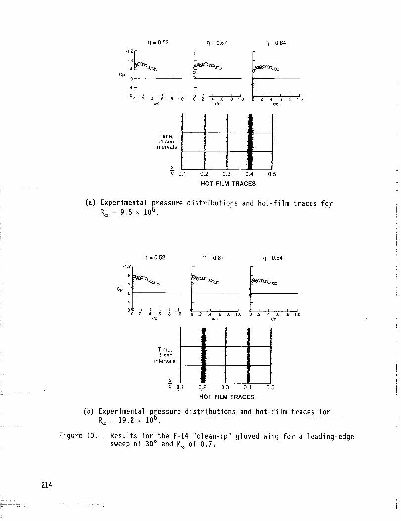
q = 0.52

Cp

8 I A I I I I

0 .2 .4 .6 .8 1.0

X/C

q = 0.67

I I l I I

.2 .4 .6 .8 1.0

_C

1"1= 0.84

.2 .4 .6 .8 t.0

x/c

Time,•1 sec

intervals

X

c 0.1

F

0•2 0,3 0.4

HOT FILM TRACES

0.5

(a) Experimental pressure distributions and hot-film traces for

R_ = 9.5 x 106 .

q = 0.52 q = 0.67 q = 0.84

Cp

.8 1 1 I _. I I

0 .2 .4 .6 .8 1.0 0 .2 .4 .6 .8 1.0 0 .2 .4 .6 .8 1_0

X/C X/C X/C

Time,.1 sec

intervals

xC- 0,1 0.2 0.3 0.4 0.5

HOT FILM TRACES

(b) Experimental pressure distributions and hot-film traces for

R= = 19.2 x 106 .

Figure 10. - Results for the F-14 "clean-up" gloved wing for a leading-edge

sweep of 30° and M_ of 0.7.

214

.6_ I Flight 4' Stati°n 3.5I S NF (Normal flow)

;tX/C .

2 _- _wlse flow)Instability_ -_

.__4 8 12 16 20 24 28

R co/106

(c) Computed transition and instability locations versus free-stream Reynoldsnumber.

Figure 10. Concluded.

215

M co_ 28 °

40 °

0

48 °

Equal_wihg areaAspect ratioTaper ratioShock sWeepShock location

Figure 11.

(a) P1anforms.

(AR = .4, Taper ratio = .4)

5O

Forward swept wing48

46

44

42

40

38

36

34

32 Aft swept wing

30

1 1 1 ! I0 .2 .4 .6 .8 1.0

x/c

(b) Local sweep variationswith respectto x/c.

Comparisonbetween "equivalent"forwardand aft swept wings.

2]6

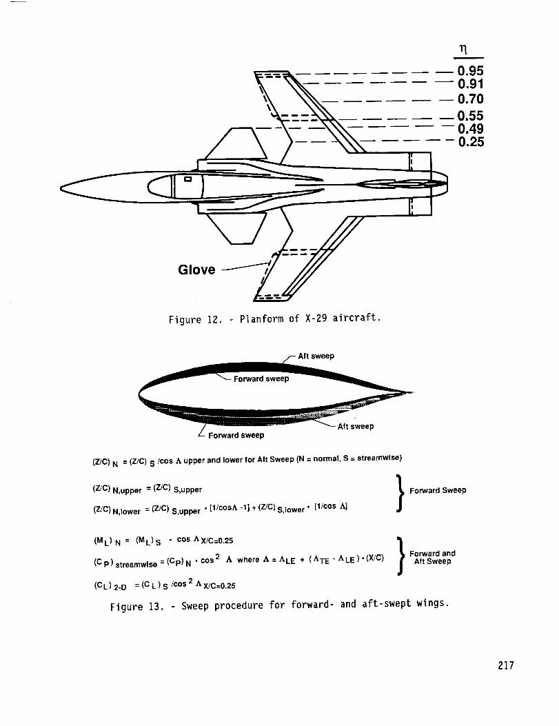
Glove

11m

0.950.910.70

0.550.490.25

Figure 12. - Planform of X-29 aircraft.

7--Aftsweep

Forwardsweep

Forward sweepAft sweep

(Z/C) N = (Z/C) S/cos A upper and lower for Aft Sweep (N = normal, S = streamwise)

(Z/C) N,upper = (Z/C) S,upper

(Z/C) N,Iower = (Z/C) S,upper " [1/cosA -1] + (Z/C) S,Iower" [1/cos A]}Forward Sweep

(ML) N = (ML)s " cos AX/C=0.25 ,_

(Cp)streamwise=(Cp)N .cos 2 A where A=ALE + (ATE-ALE).(X/C) ,_ ForwardandAft Sweep

(CL) 2-D = (C L ) S /cos 2 A X/C=0.25

Figure 13. Sweep procedure for forward- and aft-swept wings.

217

-.8 i- F- Forward-swept| / /- Aft swept

..4__0 _o- \\\\_ Experimental upper

Cp

"'02 _

Experimental lower

.4 1 I I I I I I 1 I I0 .1 .2 .3 .4 .5 .6 .7 .8 .9 1.0

Figure i4.

X/C

Computational results for the pressure distributions on the

X-29 wing section situated on both forward and aft wings.

(M_ = 0.91, n = 0.70, ALE = 30 °)

i

218

X/C

.4

.3

.2

Transition

NF (Normal flow) -_

SF (Spanwise flow) -_

F

8 12 16 20 24 28

R=o/10 6

(a) Transition location versus R_.

C D wake

10-4

44

40

36

32

28

24

20

B

I I I J I8 12 16 20 24 28

Rco/10 6

(b) CDwak e for baseline versus R_ and comparison with NLF-Glove.

Figure 15. Computed results for X-29 baseline section for n = 0.7,

M= = 0.91.

219

A LE = 300

Y/C

.03 NLF-GIove _ "_.

.02Baseline

.01

\0

-.01

Figure 16.

-.02

-.03

-.04 l 1 I I0 .2 .4 .6 .8 1.0

X/C

Comparison between baseline geometry and NLF-Glove for X-29 wingfor _ = 0.7.

220

Cp

-.8

-.6

-.4

-.2

0

Baseline (C L = 0,351)

C p(Sonic)

\

NLF-GIove

(C L = 0.435).2

.4 1 1 I J I0 .2 .4 .6 .8 1.0

X/C

(a) Comparison between baseline and NLF-GIove for M= : 0.905 and leading-edgesweep of 30°

mm 8 m

-.6

-,4

C p -.2

0

.2

• 4 I I I L I I I l l . J0 .2 .4 .6 .8 1.0

X/C

(b) Pressure distribution for M_ = 0.865 and leading-edge sweep of 25°.

Figure 17. Chordwise pressure distributions for X-29 wing section for

= 0.7 and transition location computations.

22]

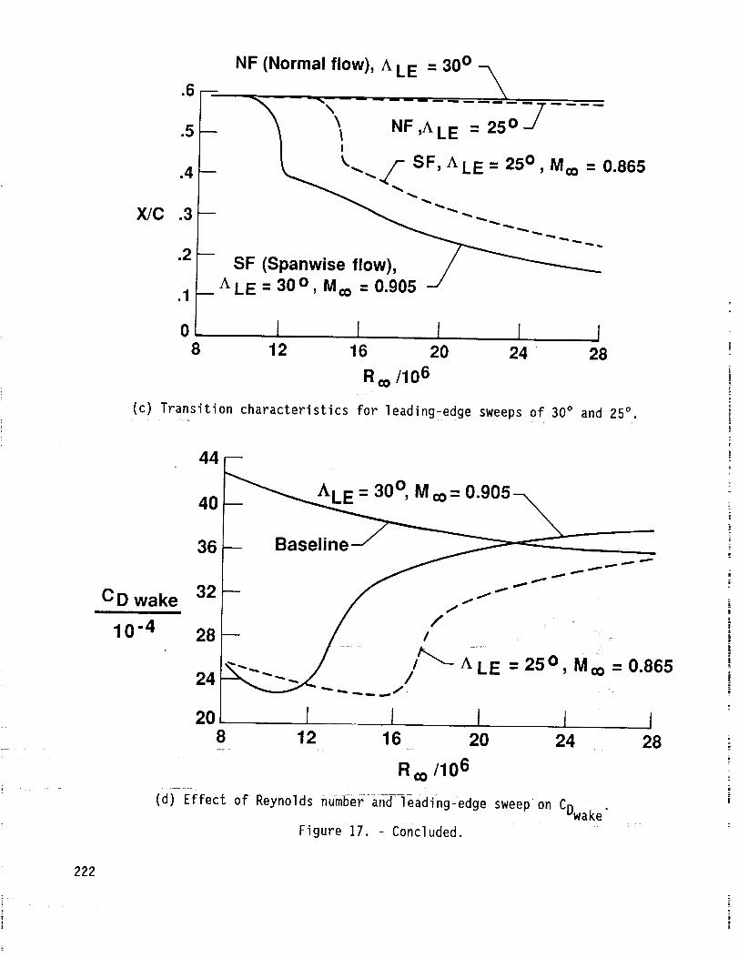
.6--

.5

.4

X/C .3

.2

.1

08

NF (Normal flow), ALE = 300 -_

---------I I J I I

12 16 20 24 28

Ro=/106

(c) Transition characteristics for leading-edge sweeps of 30° and 25° .

C D wake

10-4

44

40

36

32

28

24

208

(d)-;Effect of

ALE = 30 °, M Qo= 0.905

Baseline

//

/

i 1 I J12 16 20 24

i t''-- ALE = 25 o, M o_ = 0.865

R oo/106

Reynolds number and-ieading-edge sweep on CDwak e.

Figure 17. - Concluded.

I28

222

-.8--- 1"1= .49-7 r 1"1= .70

Cp, upper -.4

o I(a) Constant spanwise pressure gradient.

-.8

Cp, upper -.4

0

I-" 11 149

--A C p 1"1= .70 7 /

• • , • " • • - •

1 I I I I 1, I 1 I \1.2 .4 .6 .8 1.0

X/C

(b) Linearly varying spanwise pressure gradient•

Figure 18. - Schematics showing types of spanwise pressure gradients studied.

223

(M Go= 0.905, A LE = 30 o)

NF,ACPc = .15 7/

NF (Normal flow), A C Pc=0 --_ /

.6 _- ............ -,, -, _

_._ ",.5 -- _SF,ACp = .15 \ "-../

X/C .3 - "--..

.2 -- o_SF (Spanwise fl

.1 --

o i t 1 I I8 12 16 20 24 28

R oo/106

Figure 19. - Comparison of the effect of a constant spanwise pressure

gradient of ACPc = 0.15 on transition with that for zero

spanwise gradient, i.e., with ACPc = O.

40

(M =o= 0.905, A LE = 30 o)

36

32C D wake

10-4

ACpc=°.05 -_ "" //

/ /

8 12 16 20 24

R ¢o/106

Figure 20. - CDwak e versus R_ with ACPc as parameter for X-29 glove.

28

224

(Moo = 0.905, ALE = 30 o )

NF (Normal flow), A C PI = 0

.6

.5

.4

X/C .3

.2

.1

0

..... -.,, ._.7... ../-:F ,_CPi = .15

-_ \ "-- .......,.

-.SF, _CPi = .15

SF (Spanwise flow), ,_ C PI = 0

8I 1 I l 1

12 16 20 24 28

R co/106

Figure 21. - Effect of linear spanwise pressure gradient of aCPl = 0.15 on

transition characteristics of X-29 glove and comparison with

ACP1 = O.

(M oo= 0.905, ALE = 300)

C D wake

10-4

40|F-- ACPI =0 -_ ____

36}-- .o5_-_ _f''__-L__'-

28/ / /:" : _-.lO2__ ///Q._

8 12 • 16 20 24 28

Roo/106

Figure 22. - CDwak e versus R_ with aCp as parameter for X-29 glove.l

225

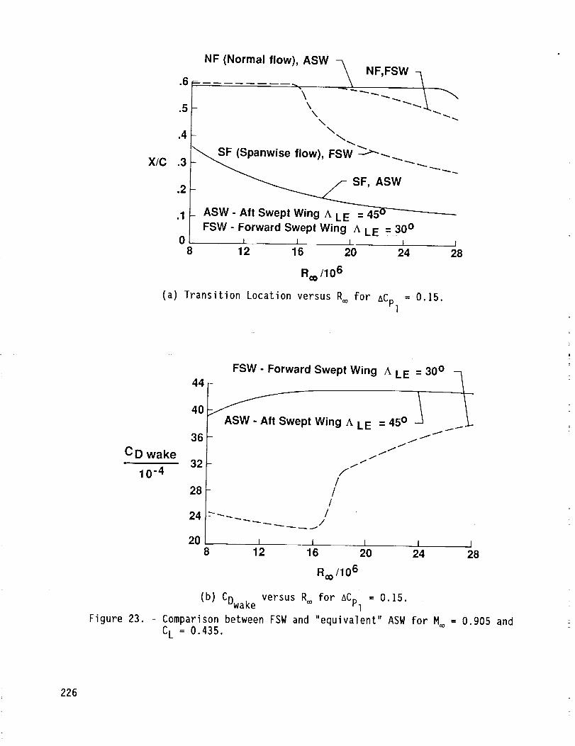
X/C

.6=-

,5 -

.4

.3

.2

.1

08

NF (Normal flow), ASW -_ NF, FSW -_

N\

__anwise flow), FSW _'_._ __....

_ _ASW -

i ASW - Aft Swept Wing A L E = 45°-----------_

FSW - Forward Swept Wing ALE = 300I 1 l I •

12 16 20 24 28

R=o/106

(a) Transition Location versus R= for aCp] = 0.15.

C D wake

10-4

Figure 23.

44

40

36

32

28

24

20

FSW - Forward Swept Wing ALE = 30o

"A__SW • Aft Swept Wing A LE = 450 -_

ff

f7

f

f/

//

/

I J12 16

Roo/106

I J I8 20 24 28

(b) CDwak e versus R= for ACPl = 0.15.

Comparison between FSW and "equivalent" ASW for M= = 0.905 and

CL = 0.435.

226

.6

.5

.4

X/C .3

.2

.1

0

NF (Normal flow), ASW -,_

-_ \\ ---__..._. _ NF,FSW

"__ \_SF (_anwise flow), FSW

SF, ASW -J _ ""-_-.. _.

- ASW - Aft Swept Wing A I.E = 45o

- FSW - Forward Swept Wing A LE = 30o

I I I I I

8 12 16 20 24 28

Roo/106

(c) Transition location versus R_ for ACPl = -0.15.

C D wake

10-4

44-

4O

36

32

28

24

20

//

w

8

Forward Swept Wing A LE = 300 -_

Aft Swept Wing A LE

JJ

JJ

tf

f

f

1 1 I I J

20 24 2816

Roo/106

(d) CDwake versus R_ for ACPl -0.15.

Figure 23. - Concluded.

227