multiple time scales in survival analysis
TRANSCRIPT
Multiple Time Scales in Survival Analysis
by
Thierry Duchesne
A thesis
presented to the University of Waterloo
in ful�lment of the
thesis requirement for the degree of
Doctor of Philosophy
in
Statistics
Waterloo, Ontario, Canada, 1999
c Thierry Duchesne 1999

I hereby declare that I am the sole author of this thesis.
I authorize the University of Waterloo to lend this thesis to other institutions or
individuals for the purpose of scholarly research.
I further authorize the University of Waterloo to reproduce this thesis by photocopying
or by other means, in total or in part, at the request of other institutions or individuals
for the purpose of scholarly research.
ii

The University of Waterloo requires the signatures of all persons using or photocopying
this thesis. Please sign below, and give address and date.
iii
Abstract
Multiple Time Scales in Survival Analysis
In many survival analysis applications, there may not be a unique plausible scale
in which to measure time to failure or assess performance. This is especially the case
when several measures of usage or exposure are available on each unit or individual. For
example, the age, the total number of ight hours, and the number of landings are usage
measures that are often considered important in aircraft reliability. This thesis considers
the de�nition of a "good" time scale, along with models that combine di�erent usage
or exposure measures into a single scale. New semiparametric inference methods for
these models are developed and their e�ciency in moderate size samples is investigated.
Datasets are used to illustrate the implementation of these methods and of some model
assessment procedures. Ideas for further applications and research are also given.
iv

Acknowledgements
It would be impossible for me to thank all the nice people who have helped me in numerous
ways during my doctoral studies at the University of Waterloo. However, I must take the
time to express my gratitude to the main contributors to this work.
First and foremost, I wish to thank my supervisor, Professor Jerry Lawless, for his
guidance during these years. Not only did he provide me with �nancial and moral sup-
port, but he also introduced me to a very interesting topic. I consider myself extremely
fortunate to have bene�ted from his knowledge and experience, and without his help this
work would not have been possible.
I also wish to thank Professors Richard Cook, Yigal Gerchak, John Kalb eisch, Jock
MacKay and William Meeker (Iowa State University) for agreeing to be on my thesis
committee. The time they have devoted to read my thesis and their helpful feedback is
much appreciated.
I must also thank Professors Don McLeish and Mary Thompson for answering some
of my questions, for loaning me some of their textbooks and for writing reference letters
for me.
Thank you to Josianne, for your patience while I was working on this project far away
from you. Being apart from somebody as special to me as you are undoubtedly motivated
me to work harder.
Thanks to my family, whose support was always there when I needed it.
Finally, I wish to thank the National Sciences and Engineering Research Council of
Canada for supporting this research with a Postgraduate Scholarship.
v

Contents
1 Introduction 1
1.1 Time scales . . . . . . . . . . . . . . . . . . . . . . . . . . . . . . . . . . 3
1.2 Ideal time scales . . . . . . . . . . . . . . . . . . . . . . . . . . . . . . . . 8
1.3 Properties of ideal time scales . . . . . . . . . . . . . . . . . . . . . . . . 11
1.4 Uses and applications of ideal time scales . . . . . . . . . . . . . . . . . . 14
2 Families of models 18
2.1 Transfer functional models . . . . . . . . . . . . . . . . . . . . . . . . . . 19
2.2 Hazard based models . . . . . . . . . . . . . . . . . . . . . . . . . . . . . 20
2.2.1 Multiplicative hazards model . . . . . . . . . . . . . . . . . . . . 21
2.2.2 Additive hazards model . . . . . . . . . . . . . . . . . . . . . . . 22
2.3 Time transformation models . . . . . . . . . . . . . . . . . . . . . . . . . 23
2.4 Collapsible models . . . . . . . . . . . . . . . . . . . . . . . . . . . . . . 26
3 Parametric estimation for collapsible models 31
3.1 Parametric usage paths . . . . . . . . . . . . . . . . . . . . . . . . . . . . 32
3.2 Multiplicative scale model . . . . . . . . . . . . . . . . . . . . . . . . . . 33
3.3 Linear scale model . . . . . . . . . . . . . . . . . . . . . . . . . . . . . . 34
vi

3.3.1 Parameterization . . . . . . . . . . . . . . . . . . . . . . . . . . . 35
3.4 Maximization of the likelihood . . . . . . . . . . . . . . . . . . . . . . . . 39
3.5 Asymptotic properties . . . . . . . . . . . . . . . . . . . . . . . . . . . . 40
3.6 Missing information . . . . . . . . . . . . . . . . . . . . . . . . . . . . . . 42
4 Semiparametric inference for collapsible models 44
4.1 Minimum coe�cient of variation . . . . . . . . . . . . . . . . . . . . . . . 46
4.1.1 Separable scale model . . . . . . . . . . . . . . . . . . . . . . . . 47
4.1.2 General collapsible model . . . . . . . . . . . . . . . . . . . . . . 51
4.1.3 Censored observations . . . . . . . . . . . . . . . . . . . . . . . . 52
4.1.4 Variance estimate . . . . . . . . . . . . . . . . . . . . . . . . . . . 54
4.2 Quasi-likelihood . . . . . . . . . . . . . . . . . . . . . . . . . . . . . . . . 56
4.2.1 Separable scale model . . . . . . . . . . . . . . . . . . . . . . . . 57
4.2.2 General collapsible model . . . . . . . . . . . . . . . . . . . . . . 62
4.2.3 Censored observations . . . . . . . . . . . . . . . . . . . . . . . . 62
4.3 Rank based methods . . . . . . . . . . . . . . . . . . . . . . . . . . . . . 62
4.3.1 General collapsible model . . . . . . . . . . . . . . . . . . . . . . 63
4.3.2 Asymptotic properties . . . . . . . . . . . . . . . . . . . . . . . . 65
4.3.3 Separable scale model . . . . . . . . . . . . . . . . . . . . . . . . 68
4.3.4 Application of the method . . . . . . . . . . . . . . . . . . . . . . 69
4.4 Simulation study . . . . . . . . . . . . . . . . . . . . . . . . . . . . . . . 70
4.4.1 Linear scale model . . . . . . . . . . . . . . . . . . . . . . . . . . 71
4.4.2 Multiplicative scale model . . . . . . . . . . . . . . . . . . . . . . 82
4.4.3 Non separable scale model . . . . . . . . . . . . . . . . . . . . . . 88
4.4.4 Variance estimates and con�dence intervals . . . . . . . . . . . . . 92
vii
4.4.5 Censored data simulations . . . . . . . . . . . . . . . . . . . . . . 95
4.4.6 Simulation summary . . . . . . . . . . . . . . . . . . . . . . . . . 97
5 Some other methods and applications 99
5.1 Ideas for nonparametric inference . . . . . . . . . . . . . . . . . . . . . . 99
5.1.1 Method based on grouped usage paths . . . . . . . . . . . . . . . 100
5.1.2 Nonparametric quantile regression . . . . . . . . . . . . . . . . . . 102
5.2 Applications of the collapsible model . . . . . . . . . . . . . . . . . . . . 103
5.2.1 Maintenance programs . . . . . . . . . . . . . . . . . . . . . . . . 104
5.2.2 Prediction . . . . . . . . . . . . . . . . . . . . . . . . . . . . . . . 105
5.2.3 An example of application: the warranty cost . . . . . . . . . . . 106
5.2.4 Accelerated testing . . . . . . . . . . . . . . . . . . . . . . . . . . 108
6 Data analysis and model assessment 110
6.1 Fatigue life of steel specimens . . . . . . . . . . . . . . . . . . . . . . . . 110
6.2 Fatigue life of aluminum specimen . . . . . . . . . . . . . . . . . . . . . . 120
6.3 Cracks in the joint unit of the wing and fuselage . . . . . . . . . . . . . . 124
6.4 Failure times and mileages for tractor motors . . . . . . . . . . . . . . . . 127
7 Conclusion 131
A Datasets 135
A.1 Fatigue life of steel specimen data . . . . . . . . . . . . . . . . . . . . . . 135
A.2 Fatigue life of aluminum specimen . . . . . . . . . . . . . . . . . . . . . . 137
A.3 Cracks in the joint unit of the wing and the fuselage . . . . . . . . . . . . 139
A.4 Failure times and mileages for tractor motors data . . . . . . . . . . . . . 141
viii

List of Tables
3.1 True and estimated values of Pr [X > xj�] with model (3.13). . . . . . . . 39
4.1 Percentiles of real time at failure given usage path, Batch 1 . . . . . . . . 72
4.2 Simulation results, linear scale model, Batch 1. . . . . . . . . . . . . . . . 72
4.3 Percentiles of real time at failure given usage path, Batch 2 . . . . . . . . 74
4.4 Simulation results, linear scale model, Batch 2. . . . . . . . . . . . . . . . 74
4.5 Percentiles of real time at failure given usage path, Batch 3 . . . . . . . . 75
4.6 Simulation results, linear scale model, Batch 3. . . . . . . . . . . . . . . . 75
4.7 Percentiles of real time at failure given usage path, Batch 4 . . . . . . . . 77
4.8 Simulation results, linear scale model, Batch 4. . . . . . . . . . . . . . . . 77
4.9 Simulation results, linear scale model, Batch 5. . . . . . . . . . . . . . . . 79
4.10 Simulation results, linear scale model, Batch 6. . . . . . . . . . . . . . . . 80
4.11 Simulation results, linear scale model, Batch 7. . . . . . . . . . . . . . . . 81
4.12 Simulation results, linear scale model, Batch 8. . . . . . . . . . . . . . . . 81
4.13 Percentiles of real time at failure given usage path, Batch m1 . . . . . . . 83
4.14 Simulation results, multiplicative scale model, Batch 1. . . . . . . . . . . 83
4.15 Percentiles of real time at failure given usage path, Batch m2 . . . . . . . 84
4.16 Simulation results, multiplicative scale model, Batch 2. . . . . . . . . . . 84
ix

4.17 Percentiles of real time at failure given usage path, Batch m3 . . . . . . . 85
4.18 Simulation results, multiplicative scale model, Batch 3. . . . . . . . . . . 85
4.19 Percentiles of real time at failure given usage path, Batch m4 . . . . . . . 86
4.20 Simulation results, multiplicative scale model, Batch 4. . . . . . . . . . . 86
4.21 Simulation results, multiplicative scale model, Batch 5. . . . . . . . . . . 86
4.22 Simulation results, multiplicative scale model, Batch 6. . . . . . . . . . . 87
4.23 Simulation results, multiplicative scale model, Batch 7. . . . . . . . . . . 87
4.24 Simulation results, multiplicative scale model, Batch 8. . . . . . . . . . . 88
4.25 Simulation results, nonseparable scale model, Batch 1. . . . . . . . . . . 90
4.26 Simulation results, nonseparable scale model, Batch 2. . . . . . . . . . . 91
4.27 Simulation results, nonseparable scale model, Batch 3. . . . . . . . . . . 91
4.28 Simulation results, nonseparable scale model, Batch 4. . . . . . . . . . . 91
4.29 Coverage of 95% con�dence intervals, quasi-likelihood . . . . . . . . . . . 93
4.30 Coverage of 95% con�dence intervals, minimum CV . . . . . . . . . . . . 93
4.31 Coverage proportion . . . . . . . . . . . . . . . . . . . . . . . . . . . . . 94
4.32 Simulations results, censored samples. . . . . . . . . . . . . . . . . . . . . 96
4.33 Coverage of rank score based 95% con�dence intervals, censored samples. 96
6.1 Linear scale parameter estimates, Kordonsky and Gertsbakh (1995a) data. 111
6.2 Multiplicative scale parameter estimates, Kordonsky and Gertsbakh (1995a)
data. . . . . . . . . . . . . . . . . . . . . . . . . . . . . . . . . . . . . . . 112
6.3 Multiplicative scale parameter estimates, Kordonsky and Gertsbakh (1995a)
data. . . . . . . . . . . . . . . . . . . . . . . . . . . . . . . . . . . . . . . 113
6.4 Chi-squared goodness-of-�t test, Kordonsky and Gertsbakh (1995a) data. 120
x

A.1 Fatigue life of 30 steel specimens. . . . . . . . . . . . . . . . . . . . . . . 136
A.2 Description of the 7 di�erent usage paths . . . . . . . . . . . . . . . . . . 137
A.3 Block number and cumulative number of cycles at failure. . . . . . . . . . 138
A.4 Number of cracks in wing joints and number of landings at inspection. . . 139
A.5 Failure times and mileages of 40 traction motors. . . . . . . . . . . . . . 141
xi
List of Figures
1.1 Examples of usage paths . . . . . . . . . . . . . . . . . . . . . . . . . . . 6
2.1 Example of age curves generated by an ITS in a collapsible problem . . . 27
3.1 Pro�le log-likelihoods of � for typical samples from models (3.12) and (3.11). 38
3.2 Contours of the log-likelihood evaluated at �2 = 1 and pro�le log-likelihood
of for a typical sample from model (3.13). . . . . . . . . . . . . . . . . 39
4.1 Forms of the squared sample CV function. . . . . . . . . . . . . . . . . . 51
4.2 Typical form of the rank-based score function. . . . . . . . . . . . . . . . 66
4.3 Percentiles of real time at failure given usage path 1 . . . . . . . . . . . . 73
4.4 Histogram, rank estimator, batches 1 and 3. . . . . . . . . . . . . . . . . 76
4.5 Impact of the observed path distribution on estimator of TS parameter. . 78
4.6 Impact of the distribution G on estimator of TS parameter. . . . . . . . 79
4.7 Shape of the usage paths for the model used in Section 4.4.3. . . . . . . . 89
4.8 CV 2[T (�)] as a function of �, non separable scale model . . . . . . . . . . 90
5.1 Age surfaces drawn using nonparametric algorithm. . . . . . . . . . . . . 101
6.1 Failure times versus path features, scale T = X + 6:7y(X). . . . . . . . . 114
xii

6.2 Failure times versus path features, scale T = X + 6:7y(X). . . . . . . . . 115
6.3 Failure times versus path features, scale T = X0:205y(X)0:795. . . . . . . . 116
6.4 Failure times versus path features, scale T = X0:455y(X)0:545. . . . . . . . 117
6.5 Weibull and lognormal probability plots, scale T = X + 6:7y(X). . . . . . 118
6.6 Weibull and lognormal probability plots, scale T = X0:205y(X)0:795. . . . 119
6.7 Failure times vs path number, approach 1 . . . . . . . . . . . . . . . . . 121
6.8 Failure times vs path number, approach 2 . . . . . . . . . . . . . . . . . 122
6.9 Number of cycles�amplitude versus number of cycles at failure. . . . . . 123
6.10 Pro�le log likelihood of the time scale parameter, linear scale model . . . 125
6.11 Pro�le log likelihood of the time scale parameter, multiplicative scale model126
6.12 Mileage (miles) versus time (days) at failure for the locomotive traction
motor data of Singpurwalla and Wilson (1995). . . . . . . . . . . . . . . 128
6.13 Rank score for the linear scale with the locomotive traction motor data. . 128
6.14 Rank score for the multiplicative scale with the locomotive traction motor
data. . . . . . . . . . . . . . . . . . . . . . . . . . . . . . . . . . . . . . . 129
xiii
Chapter 1
Introduction
In many survival analysis applications, there may not be a unique plausible scale in
which to measure time until failure or assess performance. This is especially the case
when several measures of usage or exposure (such as the total number of cycles, the
cumulative exposure to some risk, etc.) are available on each unit. The most classic
example of such a situation is an automobile warranty, where both cumulative mileage
and time since purchase are virtually always considered1. Even though it is easier to
think of problems arising from engineering, multiple time scales are also quite useful
to model certain situations in biostatistics. For example, the cumulative exposure to
pollution or the time since a �rst tumor may provide more information on the time-to-
event distribution than calendar age itself.
Since most survival analysis methods assume that a time scale is already available,
it is of obvious importance to come up with a \good" scale for each problem. In order
to do so, a de�nition of \good" time scale and, in such cases, a statistical method for
1At least this is the case in North America.
1

CHAPTER 1. INTRODUCTION 2
�nding such a scale are required. But how should one de�ne a \good" time scale? For
one thing, a good time scale should preserve most of the \useful" information contained
in the available usage measures. In the words of Farewell and Cox (1979), \we look for
a time scale that accounts for as much of the variation as possible, in some sense". This
principle is somewhat similar to the concept of su�ciency (c.f. Cox and Hinkley (1974)),
in that we are searching for a method of reducing the dimension of the data without
losing any relevant information about the failure time distribution. In their 1979 note
on multiple time scales, Farewell and Cox do suggest a method to verify if a given scale
represents a valid dimension reduction, but they do not give a precise de�nition of good
time scale, nor do they propose any general method of �nding a good time scale
Moreover, a good scale should be such that units with the same age in that scale
have a similar survival probability, even if the values of their various usage measures are
di�erent. Kordonsky and Gertsbakh (1995a) use this very property in order to de�ne
what they term an ideal monitoring scale, or load invariant scale. Interestingly, they do
not seem to use this de�nition when they propose a method to �nd a best monitoring scale
from observed data. On the other hand, Oakes (1995) uses this desired property of good
time scales albeit in a parametric setting. He also introduces the notion of collapsibility,
which essentially implies that the probability of surviving beyond a given time is solely
determined by the value of the usage measures at that time.
The objectives of this thesis are to study what constitutes a \good" time scale in
further detail, to develop applications of alternative time scales, and to examine methods
of selecting a time scale. The development is closely tied to the study of time-varying
covariates in survival settings.
In this chapter, we will de�ne what we call ideal time scales and investigate their

CHAPTER 1. INTRODUCTION 3
properties. We will also propose uses and applications for models based on those time
scales.
1.1 Time scales
Before we give a formal de�nition of an ideal time scale, we �rst need to introduce a few
concepts and describe the situation. We assume that we study a population of similar
devices (brake pads, aircraft, animals or human beings, for example) that are used under
di�erent conditions. Along with the age in real time, we also observe several other
measures of cumulative usage on each unit. We want to use this available information in
order to estimate the distribution of time to failure for the devices under study. Let us
now introduce some notation.
Let X be the random variable (rv) of real time to failure. Unless otherwise speci�ed,
we assume that X is a non-negative random variable. In what follows, x � 0 will represent
real time, and sometimes also a realization of X.
De�nition 1.1 We say that y(x) is a usage measure (or usage marker) if the mapping
x! y(x) is left-continuous and if, for any two real times x1; x2 � 0 such that x1 > x2,
y(x1) � y(x2), i.e. y(�) is a left-continuous, non-decreasing function of real time.
If p di�erent usage measures are available at time x, we denote them by y1(x), y2(x), : : :,
yp(x). For convenience, we let y0(x) = x and de�ne the rv's Y
i= y
i(X), i = 0; 1; : : : ; p.
In a similar fashion, we put yi= y
i(x), i = 0; 1; : : : ; p. Finally, we let Y; y and y(x)
denote (Y0; Y1; : : : ; Yp)t, (y0; y1; : : : ; yp)
t and (y0(x); y1(x); : : : ; yp(x))t, respectively.
Sometimes, we also wish to introduce in our model (time-varying) covariates that are not
necessarily usage measures. We denote the vector containing all the covariates, including

CHAPTER 1. INTRODUCTION 4
the usage measures y, by z. The elements of z that are not in y need not be non-decreasing
in real time; all we require is that they are left-continuous.
We can now de�ne what a usage (covariate) path (or usage [covariate] history) is.
De�nition 1.2 Let P(x) = fy(u); 0 � u < xg, where y is a vector of usage measures.
We call P(x) the usage path up to time x. When P = limx!1 P(x), we say that P is
the (whole) usage path. Finally, we denote the space of all possible usage paths, P, byIP. In a similar fashion, we de�ne Z(x) = fz(u); 0 � u < xg to be the covariate path
up to time x, we use Z = limx!1 Z(x), and we denote the space of all possible covariate
histories by Z. For convenience, we assume that P(x) � Z(x), i.e. the usage history is
just the part of the covariate history that contains only non-decreasing covariates.
In much of our theory and applications, we will consider that fy(x); x � 0g and
fz(x); x � 0g are given, i.e. we consider the covariate and usage history to be �xed
for each unit under study. In situations in which the usage paths and covariate histories
are random, this means that we will have conditioned on their realizations.
Before going any further, let us look at a few examples of usage measures and paths
that can occur in practice.
Example 1.1.1 Lawless, Hu and Cao (1995) study automobile reliability. The usage
measure they consider is the cumulative mileage, and they assume that mileage is accu-
mulated at a constant rate. Mathematically, let x represent real time measured from the
date at which the car enters service, and y(x) be the cumulative mileage at time x. Then
they assume that y(x) = �x, where � > 0 is a constant usage rate that may vary from
car to car. This type of usage path is quite common and conforms to De�nitions 1.1 and
1.2. (See path 1 in Figure 1.1.)

CHAPTER 1. INTRODUCTION 5
Example 1.1.2 Suppose we want to assess the reliability of a system that has periods
of up and down time. We could de�ne x to be real time and y(x) to represent either
cumulative up time or cumulative down time at real time x. This would describe the
up/down periods of the system completely and would still comply with De�nitions 1.1 and
1.2. (See path 2 in Figure 1.1.)
Example 1.1.3 Kordonsky and Gertsbakh (1993) consider a model for aircraft reliabil-
ity. One of the numerous usage measures considered is the cumulative number of landings.
If we let x denote real time and y(x) denote the total number of landings of an airplane at
time x, we see that this type of usage path satis�es our de�nitions. (See path 3 in Figure
1.1.)
Example 1.1.4 Sometimes, we can consider a model where a given usage measure is
just a location shift in real time. An example of this type of situation is given in Farewell
and Cox (1979) where, for each woman under study, x is her calendar age and y(x) is
the elapsed time since the birth of her �rst child. In this case, y(x) = x � a, where a is
the calendar age of the mother at the birth of her �rst child. (See path 4 in Figure 1.1.)
Example 1.1.5 The cumulative amount of pollutant an individual has been exposed to
is often considered to be an important factor in the study of certain diseases. If we let x
represent real time and y(x) be the cumulative exposure to a substance up to time x, then
this can be viewed as a usage path. Oakes (1995) uses this sort of approach to estimate
the survivor function of miners exposed to asbestos dust. (See path 5 in Figure 1.1.)

CHAPTER 1. INTRODUCTION 6
x
3
y(x)
4
5
1
2
Figure 1.1: Examples of di�erent types of usage paths seen in practice.
In most problems involving multiple time scales, the number of usage measures and
covariates available on each unit is greater than one. This is why we adopt the vector
notation described above. Here is an example.
Example 1.1.6 A company interested in the reliability of its motorcycle engines keeps
track of many usage measures on each engine: cumulative usage time (minutes), total
number of low stress cycles, total number of high stress cycles, and cumulative mileage.
In this case, we could let y0(x) = x, y1(x), y2(x), y3(x) and y4(x) represent real time (x),
cumulative usage time at real time x, cumulative number of low stress cycles at real time
x, total number of high stress cycles up to real time x, and cumulative mileage at real
time x, respectively. Let y(x) = (y0(x); y1(x); y2(x); y3(x); y4(x))t. The usage path, P(x),
is then denoted by P(x) = fy(u); 0 � u < xg.
As we have stated earlier, we wish to compute the distribution of real time to failure

CHAPTER 1. INTRODUCTION 7
under di�erent conditions. In other words, we would like to know which proportion of
its lifetime distribution a given unit has survived given its covariate history. Using the
notation of De�nition 1.2, this translates into �nding
Pr [X � xjZ(x)]; 8Z(x) 2 Z(x); 8x � 0: (1.1)
We now make this key assumption: all the covariates and usage measures in the covariate
path (the zi's and the y
i's) are external covariates, i.e. the covariate paths are determined
independently of the time to failure X. Such covariates include environmental factors such
as pollution level in the atmosphere, and usage measures whose value does not indicate
if failure as occurred or not, like cumulative mileage on a car for example. We assume in
this case that (1.1) is equal to
S0[xjZ(x)] � Pr [X � xjZ]; 8Z 2 Z; 8x � 0: (1.2)
Our concept of usage or exposure measures is that they are always external covariates.
However, in some applications, internal covariates related to the \condition" of a unit or
individual are of interest. For example, in reliability the amount of degradation or wear in
a unit may be measurable, and related to the probability of failure. If we wish to include
internal time-varying covariates in our model, conditional probabilities of the form (1.2)
with internal covariates in Z are inadequate, because we would then be conditioning on
future failure information. In that situation, a model would have to be based on the joint
conditional distribution of the failure time and the internal covariates given the whole
history of the external covariates. In more precise terms, let W(x) be the history of
the internal time-varying covariates at time x, and Z(x) be the history of the external

CHAPTER 1. INTRODUCTION 8
covariates at x. Then the model would be based on probabilities of the form
Pr [X � x; W(x) = wjZ]; 8Z 2 Z; 8w 2W(x); 8x � 0: (1.3)
For most of the discussion which follows we ignore internal covariates.
Now that we have established the basic situation and de�ned the basic concepts, we
can start working on a de�nition of ideal time scale. The �rst logical step towards our
goal is to de�ne what a time scale is. We �rst give a very general de�nition.
De�nition 1.3 We say that � is a time scale (TS) if � is a positive, real-valued func-
tional � : IR+Z! IR+ such that for every x � 0 and every Z 2 Z, �[x;Z] = �[x;Z(x)]is non-decreasing in x.
In other words, a TS is simply a functional that maps a given time x and covariate path
Z onto the non-negative real line in such a way that when the value of x increases, the
value of the time in the TS cannot decrease. From here on, we use the following notation:
we let T = �[X;Z(X)] be the r.v. of the time (in the �-scale) until failure and we let
tZ (x) = �[x;Z(x)]. Often, tZ(x) is referred to as the operational time at x.
1.2 Ideal time scales
Ideally, a good TS should enable us to compute the probability given by equation (1.1)
for a given set of external covariates z1(x); : : : ; zp(x). As a matter of fact, we base our
de�nition of an ideal time scale on this very objective.

CHAPTER 1. INTRODUCTION 9
De�nition 1.4 We say that tZ (x) de�nes an ideal time scale (ITS) if it is a TS such
that for all Z 2 Z and all x � 0,
Pr [X � xjZ] = G(t); (1.4)
where t = tZ (x) and G(�) is a strictly decreasing survivor function not depending on Z.
In other words, an ITS is any TS that is a one-to-one function of the conditional survivor
function Pr [X � xjZ].Simply put, an ITS is a TS in which we can directly compare the lifetimes of all
the devices under study, no matter what their usage paths are. An ITS is therefore an
extremely powerful tool since it allows us to analyze the lifetime of all the units with a
single, univariate lifetime distribution. Of course, this is true only when the covariate
path does not contain any internal covariates, w(x), say. In that latter case, we would
probably need scales of the form T = T [x;W(x);Z(x)] in order to model probability
(1.3). This last special case requires further research and is not considered in this thesis.
Thus, an ITS is \ideal" in the sense that the age in the ITS is the only information
necessary in order to compute probability (1.1). We can hence think of an ITS as being
\su�cient" in order to compute the age of the units. We must be careful in using the
word \su�cient" here because as we will see in Chapter 3, some additional information
is required in order to compute the likelihood when performing parametric estimation.
It is worth noting that we use the probability (1.4), i.e. the conditional probability of
X given the covariate path, to de�ne an ITS instead of the joint probability of X and Zlike some authors do (e.g., Kordonsky and Gertsbakh (1993)). The advantage of a model
based on a distribution of X conditional on the covariate path (conditional model) over a

CHAPTER 1. INTRODUCTION 10
model based on a joint distribution of X and Z (joint model) is that a speci�c covariate
path distribution is intrinsic to the joint model, whereas the conditional model does not
imply any distribution for the covariate paths. This means that a conditional model can
generate a large set of distinct joint models just by being coupled with di�erent covariate
path distributions. Hence, conditional models are more comprehensive, more informative
and more exible than joint models. For instance, the conditional framework allows for
time scale models to be used in situations where the paths are non-random or �xed by
study design, as in accelerated life testing.
Di�erent de�nitions of \good" TS are considered in the literature. For instance, Kor-
donsky and Gertsbakh (1993) de�ne the best TS to be a TS that minimizes the \distance"
from what they call the load invariant scale. Their idea of load invariant scale is the same
as our idea of ITS: the load invariant scale is a TS in which same values of the time repre-
sent the same quantile of the lifetime distribution, independently of the covariate history
(which they term load). However, their notion of a best TS is only de�ned when they
consider semiparametric or parametric estimation. They base their inference on a con-
ditional model of the form given by De�nition 1.4 when dealing with censored data, in
which case they use parametric methods and make strong assumptions on the survivor
function G. When the data are complete, they use semiparametric estimation, but their
method is based on a joint model rather than a conditional model. We will further discuss
their method in subsequent chapters. Farewell and Cox (1979) use a slightly di�erent
approach in their treatment of problems involving multiple time scales. They do not give
a precise de�nition of ITS, but rather derive a method with which they can verify that a
given TS contains enough information in order to explain the failure pattern.

CHAPTER 1. INTRODUCTION 11
1.3 Properties of ideal time scales
Let us now assume that we want to model probability (1.1) when no internal covariates
are present. Note that this can include cases in which X given Z may have a non-
zero probability mass at certain x values; for example, if equipment is turned on and
o� then there may be a non-zero probability of failure at the instant a unit is turned
on (e.g. Follmann (1990)). It is therefore convenient for general discussion to allow
Pr [X � xjZ] to have jump discontinuities. The survivor function can then be written
as (e.g. Kalb eisch and Prentice (1980, Section 1.2.3))
Pr [X � xjZ] = exp
��Z
x
0hC(ujZ) du
� Yuj�x
[1� hD(u
jjZ)]; (1.5)
where hC(ujZ) is an integrable hazard function corresponding to the continuous part
of Pr [X � xjZ] and u1; u2; : : : are the jump points for Pr [X � xjZ]. The values of
hD(u
jjZ) are the discrete hazard function components,
hD(u
jjZ) = Pr [X = u
jjX � u
j;Z]:
We can write (1.5) so as to provide an explicit ITS. We have
Pr [X � xjZ] = exp��Z
x
0hC(ujZ) du+
Zx
0log[1� h
D(ujZ)] dN(u)
�; (1.6)
where dN(u) equals 1 if a jump in Pr [X � xjZ] occurs at u, and 0 otherwise. Thus
tZ (x) = �[x;Z(x)] =Z
x
0hC(ujZ) du �
Zx
0log[1� h
D(ujZ)] dN(u) (1.7)
CHAPTER 1. INTRODUCTION 12
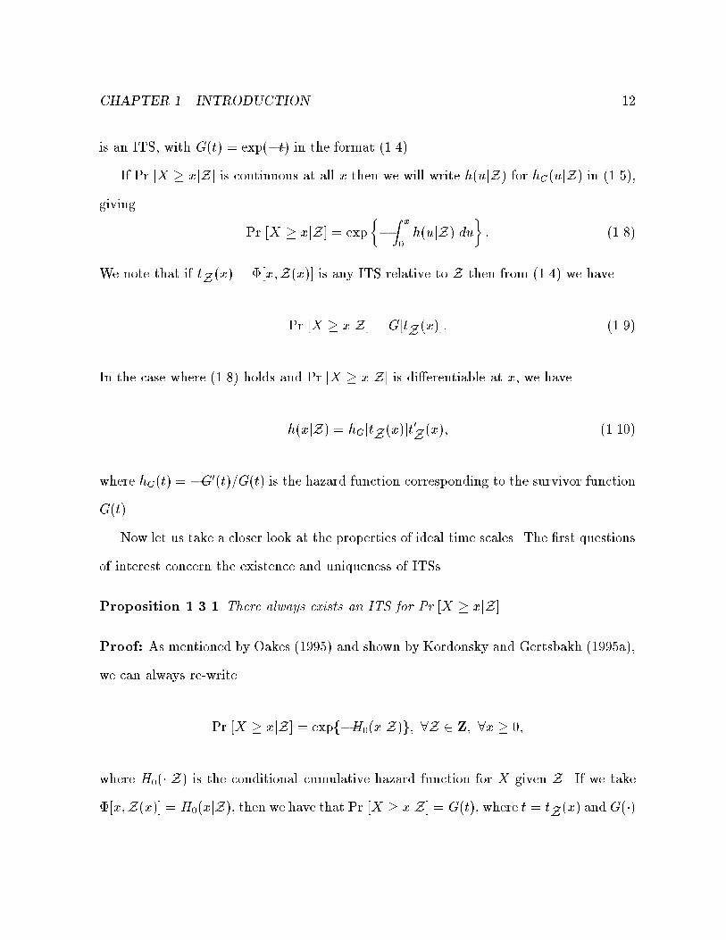
is an ITS, with G(t) = exp(�t) in the format (1.4).
If Pr [X � xjZ] is continuous at all x then we will write h(ujZ) for hC(ujZ) in (1.5),
giving
Pr [X � xjZ] = exp
��Z
x
0h(ujZ) du
�: (1.8)
We note that if tZ (x) = �[x;Z(x)] is any ITS relative to Z then from (1.4) we have
Pr [X � xjZ] = G[tZ (x)]: (1.9)
In the case where (1.8) holds and Pr [X � xjZ] is di�erentiable at x, we have
h(xjZ) = hG[tZ(x)]t0Z(x); (1.10)
where hG(t) = �G0(t)=G(t) is the hazard function corresponding to the survivor function
G(t).
Now let us take a closer look at the properties of ideal time scales. The �rst questions
of interest concern the existence and uniqueness of ITSs.
Proposition 1.3.1 There always exists an ITS for Pr [X � xjZ].
Proof: As mentioned by Oakes (1995) and shown by Kordonsky and Gertsbakh (1995a),
we can always re-write
Pr [X � xjZ] = expf�H0(xjZ)g; 8Z 2 Z; 8x � 0;
where H0(�jZ) is the conditional cumulative hazard function for X given Z. If we take�[x;Z(x)] = H0(xjZ), then we have that Pr [X � xjZ] = G(t), where t = tZ(x) and G(�)

CHAPTER 1. INTRODUCTION 13
is the survivor function of a standard exponential rv. Since H0(�jZ) is non-decreasing,� is non-decreasing as well and hence ful�lls the requirements of an ITS. Note that this
argument is also valid for problems with jump discontinuities; all we have to do in this
case is use tZ (x) given by (1.7) instead of the cumulative hazard function H0 mentioned
above.
Regarding the uniqueness issue, we know, by de�nition, that ITSs are unique up to
one-to-one transformations.
The following theorem also follows immediately from the de�nition of an ITS. Its
conclusion will be especially useful for semiparametric inference and model assessment.
Theorem 1.3.2 Let �[x;Z(x)] be an ITS for Pr [X � xjZ], T = �[X;Z(X)] and
t = �[x;Z(x)]. Then for all Z 2 Z and all t = �[x;Z(x)] for some x � 02,
Pr [T � tjZ] = Pr [T � t]: (1.11)
Proof: If t = �[x;Z(x)] for a single value of x, then
Pr [T � tjZ] = Pr [X � xjZ]
= Pr [T � t];
the last equality following from the de�nition of an ITS. If t = �[x;Z(x)] for all x
in some set A, then by de�nition of an ITS, Pr [X � xjZ] remains constant for all
x 2 A and, hence, Pr [T � tjZ] = Pr [X � xjZ]. But by de�nition of an ITS,
Pr [X � xjZ] = Pr [T � t], which completes the proof.
2Values of t 6= �[x;Z(x)] for any x � 0 for a given Z are not a concern here as these values occur
with probability zero, G(�) being a strictly decreasing survivor function in De�nition 1.4.

CHAPTER 1. INTRODUCTION 14
The theorem above indicates that, with probability equal to one, the failure times in
the ITS, T = �[X;Z(X)], will be statistically independent of the covariate histories, Z,when these histories are random variables.
1.4 Uses and applications of ideal time scales
One may ask the question \Why not use one measure as the main scale and let the
other usage measures enter the model as time-varying covariates?". As mentioned in
Farewell and Cox (1979), this is the logical thing to do if one of the measures is of
primary importance. However, when numerous usage measures are available, it may not
be easy to determine which of the measures, or if a combination of those measures, is more
relevant, and because models with covariates treat the time variable and the covariates
quite asymmetrically, it is not recommended to choose an arbitrary scale as the main
time scale and the other scales as covariates. Moreover, even if a particular scale appears
to be more important than the others, the number of tractable models that can treat
time-varying covariates is limited. As mentioned earlier, time scale based models may
also possibly be used to include the information given by internal time-varying covariates.
(Unfortunately, this last issue has not been investigated thoroughly yet and remains a
potential research topic.)
One may also argue that because real world processes and their consequences occur
in \real" or chronological time, it obviously plays an important role. Nevertheless, there
are reasons for adopting an alternative time scale tZ (x) in certain contexts.
For instance, in some cases the failure process may depend primarily on tZ (x), sothat it is scienti�cally \su�cient". For example, the probability that an item survives

CHAPTER 1. INTRODUCTION 15
past a certain chronological time x may only depend on its tZ (x) value.Another important application of ITSs is what Kordonsky and Gertsbakh (1995a) call
indirect monitoring. This means the monitoring of the internal state of a system by calcu-
lating its age. Since age in real time does not usually signify much for systems used under
di�erent conditions, Kordonsky and Gertsbakh combine various usage measures into a
single TS in which they determine the age of the systems under study. Consequently,
one sees that an ITS can be very useful in designing maintenance programs, especially if
the failure distribution in this scale is concentrated over a short interval. Indeed, by the
very de�nition of an ITS, one knows that the age in the ITS implies the same quantile
of the lifetime distribution, no matter what the usage path is. This means that only
one maintenance program is necessary, as long as the times of the di�erent maintenance
operations are scheduled according to the ITS. This turns out to be quite convenient in
situations where direct monitoring of the internal state of the systems cannot be done or
can only be done at a high cost (eg: nuclear power plants or workers exposed to asbestos
dust, see Kordonsky and Gertsbakh (1995a) and Oakes (1995)). In addition, because of
the generality in their de�nition, ITSs can be used to perform indirect monitoring and
design maintenance programs in a wide range of applications. For instance, it is relatively
simple to think of TS models that can be used in situations where usage paths are of the
types discussed in Examples 1.1.1-1.1.5 and shown in Figure 1.1. We will consider such
models in detail later on.
A time scale tZ(x) also is advantageous for experimental design and decision making.
For example, if the failure pattern for some system component depends primarily on the
accumulated voltage-time, then reliability studies in which such components are tested
at very high voltage over short periods of time may be extrapolated to normal customer

CHAPTER 1. INTRODUCTION 16
usage conditions.
A further argument for using an alternative scale is that the e�ects of treatments or
covariates may be most simply or directly expressed on some scale other than real time.
Another interesting feature of ITSs is the way they can handle more complicated
censoring schemes. Such situations often occur in the analysis of warranty data (see
Lawless, Hu and Cao (1995)), where we know the exact value of the time at failure
only if the values of the usage measures are all within the warranty region at that time.
Therefore, in those cases, censoring does not provide the lower (and/or upper) bound
of an interval where failure has occurred, but rather the bounds of a multi-dimensional
region. The nice property of an ITS in that kind of setup is that it brings back the
problem to one dimension. Models based on ITSs are therefore quite useful for modeling
the distribution of time to failure when the censoring scheme is multi-dimensional.
Censoring does not only cause problems when it is multivariate; heavy censoring3 can
make statistical inference extremely ine�cient, and sometimes even almost impossible.
However, if information on the covariate path is available, then looking at the distribution
of X given Z or at the value of a given scale T = �[X;Z(X)] may turn out to be more
informative than considering the marginal distribution of X, and hence improve on the
precision and the e�ciency of the inference.
Unfortunately ITSs are not always su�cient, for example if one wants to estimate
warranty costs and calculate warranty reserves. This is due to the fact that knowledge
about the distribution of the paths has to be taken under consideration. Actually, there
are other cases in which a model for the distribution of the covariate path, Z, is relevant.3This is often the case in the study of aircraft or nuclear power plants, or any other device which, we
hope, only rarely fails.
CHAPTER 1. INTRODUCTION 17
For instance, the case where the path includes internal time-varying covariates requires
a probability model for those covariates which are internal. In fact, most applications of
ITS models (e.g. conception of maintenance schedules, calculation of warranty costs, see
Chapter 5) require knowledge of the usage path distribution if they involve prediction.
In the remainder of this thesis, we outline approaches to modeling using ideal time
scales. We classify the various ITS models in Chapter 2, and we introduce a class of
models considered by Oakes (1995) that has not been thoroughly investigated in the
literature, namely, the collapsible models. In Chapter 3, we describe parametric inference
based on maximum likelihood for collapsible models. We review the maximum likelihood
method proposed by Oakes (1995) and we discuss issues concerning parameterization
that have not been addressed in the literature in this type of framework previously.
Semiparametric inference methods for those models are covered in Chapter 4; we survey
the minimum coe�cient of variation method of Kordonsky and Gertsbakh (1993), for
which we give a proof of consistency that was lacking in the literature, and we derive quasi-
likelihood and rank-based methods that yield new estimators that are often more e�cient
than the minimum coe�cient of variation estimator and that can also handle censored
samples. New ideas for nonparametric estimation are considered in Chapter 5, along
with the problem of prediction and some applications. We apply the methods described
in Chapters 3 and 4 to various datasets and propose model assessment procedures in
Chapter 6. Finally, concluding remarks are given in Chapter 7. We remark that many
of the most important applications of time scale methods are in reliability; for a recent
exposition of this area see Meeker and Escobar (1998).

Chapter 2
Families of models
Various models that incorporate usage measures and time-varying covariates in general
are proposed in the literature. In this chapter we review the main classes of such models.
Before getting into further detail, we need to �rst introduce parametric models gen-
erally. From here on, we will assume that probability (1.1) can be written as
Pr [X � xjZ(x)] = S0[xjZ(x);�]; (2.1)
where � is a vector of unknown parameters, possibly of in�nite dimension. We also
de�ne h0(xjZ(x);�) and H0(xjZ(x);�), the hazard and cumulative hazard functions,
respectively, as follows:
h0(xjZ(x);�) = lim�x!0
Pr [X 2 [x; x+�x)jX � x;Z(x);�]�x
;
and H0(xjZ(x);�) =Z
x
0h0(ujZ(u);�) du:
18

CHAPTER 2. FAMILIES OF MODELS 19
Of course,
S0(xjZ(x);�) = exp f�H0(xjZ(x);�)g :
Let us now introduce the ITS model.
De�nition 2.1 An ideal time scale (ITS) model is a model where
S0[xjZ(x);�] = G[tZ (x;�);�]; 8Z 2 Z; x � 0; (2.2)
where G is some absolutely continuous survivor function, tZ(x;�) is an ITS as de�ned
in De�nition 1.4, and � and � are two vectors of parameters that partition �.
In practical situations, G or tZ (x) or both can be speci�ed up to a vector of parameters
or left arbitrary (i.e. � or � of in�nite dimension).
From De�nition 1.4, we know that this family of models is extremely broad. Our
interest in this chapter is to outline a few sub-classes of ITS models.
2.1 Transfer functional models
Bagdonavi�cius and Nikulin (1997) have proposed a series of regression models for problems
involving time-varying covariates (stress in their terminology). Starting from di�erential
equations that model the usage rate of what they term the resource, they obtain various
probability models for the conditional survivor function S0[xjZ(x);�], where Z is the
history of a set of external covariates. Let us look at their Model 2 (see Bagdonavi�cius
and Nikulin (1997, pp. 366-367)):

CHAPTER 2. FAMILIES OF MODELS 20
De�nition 2.2 Bagdonavi�cius and Nikulin's Model 2 speci�es the following form for
tZ (x):tZ (x) =
Zx
0 [u;Z(u)] dG�1S(u); (2.3)
where [�] is a positive, real-valued functional and S is a survivor function.
Bagdonavi�cius and Nikulin (1997) derive basic properties and also consider semiparamet-
ric estimation for such a model under di�erent conditions.
In the remainder of this chapter, we will take a closer look at two special cases of
Bagdonavi�cius and Nikulin's Model 2 that are quite useful in practice, namely the hazard
based and the time transformation models.
2.2 Hazard based models
As the name suggests, hazard based models are models in which the covariate history, Z,modi�es a so-called baseline hazard function.
De�nition 2.3 A hazard based model is a model where
h0(xjZ(x);�) = [h(x);Z(x);�]; 8Z 2 Z; x � 0; � 2 �; (2.4)
where � is the parameter space, and h(�) is a baseline hazard function that can be fully
speci�ed, speci�ed up to a vector of parameters, or left arbitrary.
This de�nition is virtually useless in practice because equation (2.4) de�nes a family of
models that is too general. Let us now consider a few special cases that are widely used.

CHAPTER 2. FAMILIES OF MODELS 21
2.2.1 Multiplicative hazards model
The class of multiplicative hazards models is one of the most popular in practice. Models
of this form have been proposed by Cox (1972) and are discussed in great detail in the
literature (see Lawless (1982), Kalb eisch and Prentice (1980) or Cox and Oakes (1984),
for example). The key feature of such models is that they are very tractable mathemati-
cally and hence allow for easy inference on � , even if h(�) is left arbitrary. Multiplicative
hazards models are also quite versatile and can be used to model a wide variety of prob-
lems.
De�nition 2.4 A multiplicative hazards model is a model where
h0(xjZ(x);�) = h(x) [Z(x);�]; 8Z 2 Z; x � 0; � 2 �; (2.5)
where [�] is a positive, real-valued function.
If we take Model 2 and let [u;Z(u)] = [Z(u);�] and G(u) = exp(�u), and if we
let S(�) be an arbitrary survivor function with corresponding hazard function h(�), weobtain from (2.3) that
S0[xjZ(x)] = exp
��Z
x
0h(u) [Z(u);�] du
�;
which is exactly the multiplicative hazards model.
Many choices for the function [�] in equation (2.5) are possible. But there is one
particular form of [�] that makes inference on � in parametric and semiparametric cases
particularly easier, namely, the log-linear form.
CHAPTER 2. FAMILIES OF MODELS 22
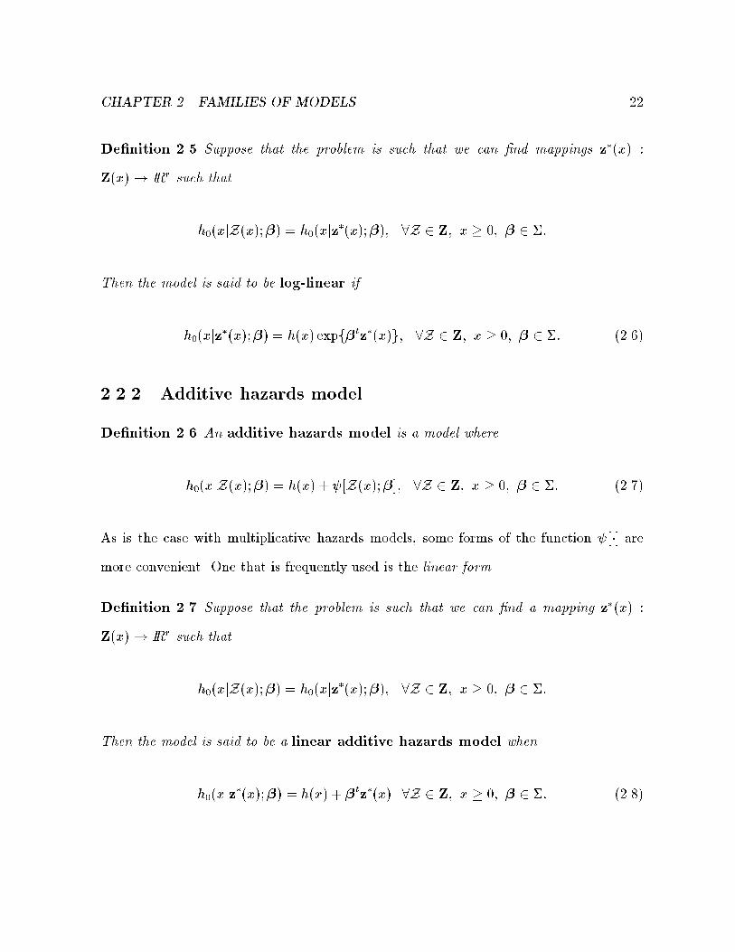
De�nition 2.5 Suppose that the problem is such that we can �nd mappings z�(x) :
Z(x)! IRr such that
h0(xjZ(x);�) = h0(xjz�(x);�); 8Z 2 Z; x � 0; � 2 �:
Then the model is said to be log-linear if
h0(xjz�(x);�) = h(x) expf�tz�(x)g; 8Z 2 Z; x � 0; � 2 �: (2.6)
2.2.2 Additive hazards model
De�nition 2.6 An additive hazards model is a model where
h0(xjZ(x);�) = h(x) + [Z(x);�]; 8Z 2 Z; x � 0; � 2 �: (2.7)
As is the case with multiplicative hazards models, some forms of the function [�] aremore convenient. One that is frequently used is the linear form.
De�nition 2.7 Suppose that the problem is such that we can �nd a mapping z�(x) :
Z(x)! IRr such that
h0(xjZ(x);�) = h0(xjz�(x);�); 8Z 2 Z; x � 0; � 2 �:
Then the model is said to be a linear additive hazards model when
h0(xjz�(x);�) = h(x) + �tz�(x) 8Z 2 Z; x � 0; � 2 �: (2.8)

CHAPTER 2. FAMILIES OF MODELS 23
Jewell and Kalb eisch (1996) use a linear additive hazards model in order to incor-
porate the information provided by marker processes into a survival distribution. They
assume that z�(x) is a (possibly multivariate) stochastic process that contains informa-
tion that may in uence the lifetime distribution, and they use a hazard function of the
form given by equation (2.8) to include that information into the model. Unfortunately,
the mathematics involved in inference procedures are quite challenging and solutions
have been obtained only in a limited number of special cases. (See Singpurwalla (1995),
Singpurwalla and Wilson (1995) or Jewell and Kalb eisch (1996) for further discussion
on this issue.)
In the case where we do not need to integrate over Z, i.e. when we condition on a
given value of the path Z, we can handle very general linear additive hazards model.
Assume that
h0(xjZ(x);�) = h0(xjz�(x);�) = �0(x;�) + �(x;�)tz�(x); 8Z 2 Z; x � 0:
Then it is possible to estimate the � functions either parametrically or nonparametrically
(see Andersen et al. (1993, Sections VII.1 and VII.4)).
2.3 Time transformation models
Despite the exibility of hazard based methods, in some situations it may be more natural
to model the e�ect of the covariate history on the survival distribution in a di�erent way.
In this section, we consider an alternate approach in which the e�ect of the covariate
path modi�es the value of the time variable instead of the value of the hazard function.

CHAPTER 2. FAMILIES OF MODELS 24
De�nition 2.8 A time transformation model (also termed accelerated failure time
(AFT) model) is an ITS model in which
tZ(x) =Z
x
0 [u; z(u);�] du; 8Z 2 Z; x � 0; (2.9)
where [�] is a positive, real-valued function.
It is more convenient to de�ne time transformation models in terms of the survivor or
cumulative hazards functions because, since they involve a change of variable of the form
U = f [X;Z(X);�], there is a di�erential element that needs to be considered in the
hazard function. In fact one can observe that equation (2.9) is equivalent to
h0(xjZ(x);�) = hG(tZ(x)) [x; z(x);�]; 8Z 2 Z; x � 0; � 2 �; (2.10)
where hG(�) is the hazard function corresponding to the survivor function G(�). One can
easily see that the AFT model is a special case of the Model 2; this is trivially observed
when one lets G = S in equation (2.3).
A common choice for [x; z(x);�] in De�nition 2.8 is
[x; z(x);�] = expfzt(x)�g:
In this log-linear case, we can see that the e�ect of the covariate path is to multiply the
value of the time variable by a certain quantity, in other words to \accelerate" time. This
category of models is very important in engineering and other domains where accelerated
life experiments are performed. One can �nd examples and a good treatment of these
experiments and models and their properties in Lawless (1982, Chapter 6), Kalb eisch

CHAPTER 2. FAMILIES OF MODELS 25
and Prentice (1980, Chapter 6) and Meeker and Escobar (1998) in the case of �xed
covariates, and in Nelson (1990, Chapter 10) and Cox and Oakes (1984, Sections 5.2
and 6.3) in the case of time-varying covariates. These authors prefer to restrict their
attention to the case in which G(�) is speci�ed up to a vector of parameters, but Robins
and Tsiatis (1992) and Lin and Ying (1995) consider a method of estimation for � in
De�nition 2.8 where G(�) can be an arbitrary survivor function.
A good example of an application of AFT models is given by Lawless, Hu and
Cao (1995), where they study the reliability of automobile brake pads from warranty
data. They use real time and cumulative mileage as their usage path. They assume that
the usage path for a given unit is of the form P(x) = f(u; �u); 0 � u < xg, where � xis the cumulative mileage at time x, i.e. � is the mileage accumulation rate that they
assume constant over time. Their model is an AFT model of the form (2.9) with, for the
ith item,
S0(xj�i;�) = G(x��i;�);8P 2 IP; x � 0; � 2 [0; 1]; � 2 �; (2.11)
where G is speci�ed up to a vector of parameters, �. An interesting property of model
(2.11) is that if � = 1, the lifetime distribution depends on the cumulative mileage only,
and if � = 0, it only depends on real time. The inference procedures for such models are
slightly complicated, in this case, by the special censoring scheme common to warranty
claim data and we refer the reader to Lawless, Hu and Cao (1995) for further information.
Another example of an application of AFT models is the problem in which a system
is either \up" or \down" (see Example 1.1.2), and failure can only occur during an \up"
period, sometimes with positive probability at the �rst moment of an up-period. If we
de�ne u(x) to be the function indicating that the system is up at time x, and if we let
NZ (x) be the cumulative number of up-time periods up to and including time x, we can
CHAPTER 2. FAMILIES OF MODELS 26
put
tZ (x) =Z
x
0u(s)f(s; z(s);�1) ds +
Zx
0k(s; z(s);�2) dNZ (s); (2.12)
where f(�) and k(�) are two positive, real-valued functions. With tZ (x) de�ned as in
(2.12), we can see that the AFTmodel can be such that failures cannot occur during down-
time and they can occur with probability masses at the beginning of up-time periods, and
this even when the survivor function G(�) is absolutely continuous; the second integral onthe right-hand side of (2.12) generates jump points in tZ(x) when x is the �rst moment
of an up-time period, and both integrals on the right-hand side of (2.12) imply that tZ (x)will stay constant when the system is down at x.
2.4 Collapsible models
In some situations, it may not be necessary to use the whole path Z in order to compute
probability (1.1). Oakes (1995) introduced the notion of collapsibility.
De�nition 2.9 Let y1(x); : : : ; yp(x) be a speci�ed set of usage factors. Then the distri-
bution of XjP is collapsible in y1(x); : : : ; yp(x) if
Pr [X > xjP] = S[y(x)]: (2.13)
In other words, in a problem collapsible in y, probability (1.1) depends on the path P(x)only through the endpoint y(x). In this case, ITS's are of the form
tP(x) = �[x; y1(x); : : : ; yp(x)] (2.14)
= �[y(x)]:
CHAPTER 2. FAMILIES OF MODELS 27
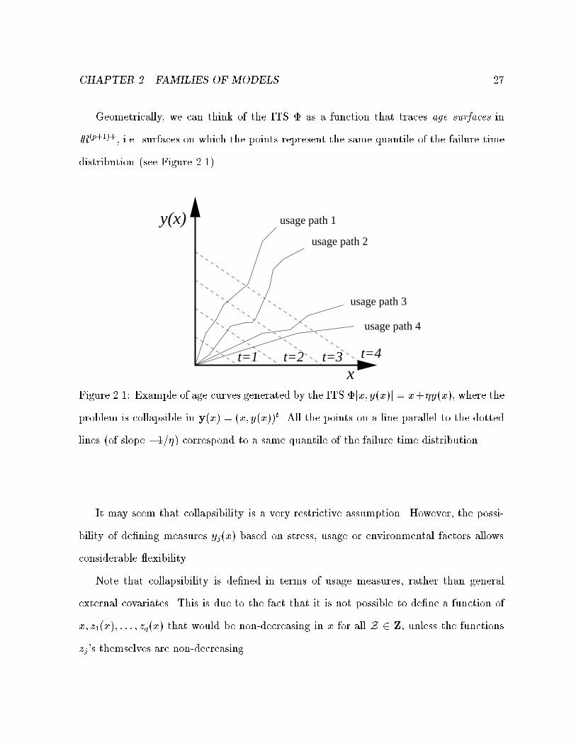
Geometrically, we can think of the ITS � as a function that traces age surfaces in
IR(p+1)+, i.e. surfaces on which the points represent the same quantile of the failure time
distribution (see Figure 2.1).
t=1
y(x)
t=2 t=3 t=4
x
usage path 1
usage path 2
usage path 3
usage path 4
Figure 2.1: Example of age curves generated by the ITS �[x; y(x)] = x+�y(x), where the
problem is collapsible in y(x) = (x; y(x))t. All the points on a line parallel to the dotted
lines (of slope �1=�) correspond to a same quantile of the failure time distribution.
It may seem that collapsibility is a very restrictive assumption. However, the possi-
bility of de�ning measures yj(x) based on stress, usage or environmental factors allows
considerable exibility.
Note that collapsibility is de�ned in terms of usage measures, rather than general
external covariates. This is due to the fact that it is not possible to de�ne a function of
x; z1(x); : : : ; zq(x) that would be non-decreasing in x for all Z 2 Z, unless the functions
zj's themselves are non-decreasing.

CHAPTER 2. FAMILIES OF MODELS 28
In some settings distinct usage paths never cross, e.g. when yj(x)'s are linear in x.
In that case all models for X given P are collapsible in the trivial sense that each Pis identi�ed by its y(x) value at any given time x. However, the ITS (2.14) is not in
general of simple functional form. The emphasis on modeling using collapsible models
is to consider fairly simple parametric speci�cations �[y(x);�] in (2.14), thus yielding
easily interpreted operational times. Oakes (1995) and Kordonsky and Gertsbakh (1993,
1995a, 1995a, 1997) consider models in which
tP(x) = �ty(x)
is assumed linear in x and y1(x); : : : ; yp(x), and G in (2.2) has a speci�ed parametric
form. Semiparametric approaches can also be adopted. For example, Kordonsky and
Gertsbakh consider a method of estimating � without a parametric model for G; this is
examined in Chapter 4.
From De�nition 2.9, we observe that a collapsible model is a special case of the class
of models de�ned by equation (2.9). Indeed, let us set
d
dxtZ (x) = [y(x);�] (2.15)
in equation (2.2) and we get a model that is collapsible, i.e. a model for which S0[xjP(x)]only depends on the value of y at x.
Collapsible models are not AFTmodels in general; the derivative on the right of (2.15)
implies that the function in the integral on the right-hand side of (2.9) would have to
be a function of both the usage measures y(x) and their derivatives y0(x).
A particular collapsible model of interest is the linear scale model.
CHAPTER 2. FAMILIES OF MODELS 29
De�nition 2.10 A linear scale model is a collapsible model such that
S(y�(x);�) = G(�ty�(x)); 8P 2 IP; x � 0; � 2 �; (2.16)
where y�(x) is a mapping y�(x) : IP(x)! IR+q, as in De�nition 2.7, and � 2 IR+q is a
vector of parameters.
A very nice property of linear scale models, along with their collapsibility, is their
interpretability.
Example 2.4.1 Suppose that x is the age in calendar years and that y(x) is the number
of packs of cigarettes smoked by an individual up to age x, and let's assume that
Pr [X � xjP(x)] = G(x+1
365y(x)); 8P 2 IP; x � 0:
Then we can say that for each pack of cigarettes smoked, an individual ages by one
day. For example, in this model, and individual aged 50 that has smoked 3650 packs of
cigarettes in his life would be \as old" as an individual aged 60 that has never smoked.
It is worth noting that the linear scale model and the additive hazard model do overlap
in some situations. Indeed, if the covariates z�(x) from De�nition 2.7 do not change sign
as x varies, we can let z��j
(x) =Rx
0 z�j
(u) du, j = 1; : : : ; q and let z��0 (x) =Rx
0 h(u) du.
This can then be re-written as a linear scale model:
S0(xjZ;�) = expn��tz��(x)
o:
Linear scale models are basically the only collapsible models used in practice so far.
Kordonsky and Gertsbakh (1993), (1995a), (1995b) and (1997b) use a linear scale model

CHAPTER 2. FAMILIES OF MODELS 30
in order to study the reliability of aircraft; Oakes (1995) employs such models to obtain
the lifetime distribution of miners exposed to asbestos dust; Farewell and Cox (1979)
investigate the time to onset of breast cancer by combining real time and time since birth
of the �rst child into a linear scale.
Another form of collapsible models that has been used in the literature is the multi-
plicative scale model.
De�nition 2.11 A multiplicative scale model is a collapsible model such that
S(y�(x);�) = G(y�0(x)�0y�1(x)
�1 � � � y�q(x)�q); 8P 2 IP; x � 0; � 2 �; (2.17)
where y�(x) is a mapping y�(x) : IP(x) ! IR+q, as in De�nition 2.7, and �0; �1; : : : ; �q
are model parameters.
Unfortunately, there is virtually no mention of other forms of collapsible models in
the current literature. Moreover, techniques of inference for the parameter � in equation
(2.16) in the rather simple case of linear scales need to be re�ned, especially in the
semiparametric setup (i.e. when G(�) is left arbitrary in (2.16)). We will try to �ll this
gap in Chapters 3 and 4 where we consider inference methods for collapsible models in a
relatively general setting. We will also brie y explore the potential of collapsible models
for prediction problems in Chapter 6.

Chapter 3
Parametric maximum likelihood
estimation for collapsible models
Parametric estimation for the collapsible models of Section 2.4 is easy to implement. In
this chapter we review maximum likelihood (ML) inference for the time scale parameters
when a fully parametric model is speci�ed. More precisely, we describe how to estimate
� and � in the collapsible model
Pr [X > xjP] = G[tP(x;�);�]; x > 0;8P 2 IP; (3.1)
where � is the vector of time scale parameters and � is the vector of parameters of the
survivor function G. Of course, model (3.1) assumes that tP(x;�) is an ITS for some �.
A �rst treatment of ML estimation for collapsible models was given by Oakes (1995).
He showed that for a set of n observations (x1;P1; �1); : : : ; (xn;Pn; �
n), where �
iis 1 if
xiis a failure time and 0 if x
iis right-censored, the likelihood function under the model
31

CHAPTER 3. PARAMETRIC ESTIMATION FOR COLLAPSIBLE MODELS 32
(3.1) is
L(�;�) =nYi=1
nfG[tPi(xi;�)]t
0
Pi(x
i)o�i
G[tPi(xi;�)]1��i
=nYi=1
n�G0[tPi(xi;�)]t0Pi(xi)
o�i
G[tPi(xi;�)]]1��i; (3.2)
where fG(t) = �G0(t) is the density corresponding to G(t) and t0
P(x) = dtPi(x)=dx. Note
that (3.1) involves t0Pi(xi) which itself usually involves y0i(x
i), even though the model is
collapsible in yi(x
i).
3.1 Parametric usage paths
We sometimes make the assumption that the usage paths can be completely speci�ed by a
�nite-dimensional vector of parameters, say �. This assumption somewhat simpli�es the
calculations and, as we will see in the following chapters, makes semiparametric inference
and model assessment easier to handle. In more precise terms, we assume that
P = fy(u);u � 0g = P(�);
where � is a vector of observed parameters that entirely describes P. In this case, we
observe (x1;�1; �1); : : : ; (xn;�n; �n) and wish to estimate � and � in
Pr [X > xjP] = Pr [X > xj�] = G[t�(x;�);�]: (3.3)
In many cases, the parametric path representation is very reasonable. For example,
Lawless, Hu and Cao (1995) consider usage paths of the form P = f(x; y(x));x � 0g,

CHAPTER 3. PARAMETRIC ESTIMATION FOR COLLAPSIBLE MODELS 33
where x is the age of an automobile in days since purchase and y(x) is the accumulated
mileage on that automobile at time x. They make the assumption that y(x) = �x,
� > 0. Their underlying assumption is, thus, that the rate of mileage accumulation on
an automobile is constant over time, which is usually close to reality during the warranty
period.
Of course, we may not be able to observe the �ivalues directly in practice. Nev-
ertheless, we can usually compute or estimate the value of the �i's from the data. For
instance, Lawless, Hu and Cao (1995) observed the values xiand y
iat failure and used
�i= y
i=x
i. If the usage path is of the form y(x) = f(x; �1; �2), then, obviously, we need
more than a single observation per usage path in order to get a unique value of (�1; �2).
3.2 Multiplicative scale model
A collapsible model encountered in the literature is the multiplicative scale model. In
certain setups, this model is equivalent to the accelerated failure time model (e.g., Lawless,
Hu and Cao (1995)). The multiplicative scale model is the one in which
Pr [X > xjP] = G[x�0y1(x)�1 � � � y
p(x)�p;�]; x > 0; 8P 2 IP: (3.4)
If we restrict ourselves to the case where there is only one usage measure of the form
y(x) = �x, then model (3.4) becomes
Pr [X > xjP] = Pr [X > xj�] = G[x��;�]; (3.5)
which is simply the accelerated failure time model.

CHAPTER 3. PARAMETRIC ESTIMATION FOR COLLAPSIBLE MODELS 34
Direct application of equation (3.2) gives a simple formula of the likelihood for model
(3.5):
L(�;�) =nYi=1
f�G0(xi��
i;�)�
�
ig�i G(x
i��
i;�)1��i: (3.6)
The multiplicative scale model seems to yield more stable estimators of � than the
linear scale model of the next section. The asymptotic variances obtained in Section 3.5
will con�rm this last statement.
3.3 Linear scale model
Let us now introduce a particular collapsible model that has been considered a few times
(e.g. Oakes (1995), Kordonsky and Gertsbakh (1997b)) in the literature, namely, the
linear scale model:
Pr [X > xjP] = G[�ty(x);�]; x > 0; 8P 2 IP: (3.7)
The likelihood function for � and � is obtained directly from (3.2):
L(�;�) =nYi=1
n�G0[�ty
i(x
i);�]�ty0
i(x
i)o�i
G[�tyi(x
i);�]1��i; (3.8)
where y0i(x) = dy
i(x)=dx. A further simpli�cation is possible when the accumulation rate
is constant for each usage measure, i.e. yi(x) = �
ix:
L(�;�) =nYi=1
n�G0[�t�
ixi;�]�t�
i
o�i
G[�t�ixi;�]1��i: (3.9)

CHAPTER 3. PARAMETRIC ESTIMATION FOR COLLAPSIBLE MODELS 35
3.3.1 Parameterization
An important issue in parametric estimation is the parameterization. Indeed, ambiguities
between the parameters in � and � in (3.1) can arise. Furthermore, even when two
parameters are not confounded it may be nearly impossible to estimate them separately
in some cases. We will explain this through an example.
Suppose that we observe n failure times x1; : : : ; xn along with n paths of the form
yi(x) = �
ix. We wish to �t the collapsible model
Pr [Xi> x
ij�i] = exp
8<:�"xi(1 + ��
i)
�1
#�2
9=; ; (3.10)
i.e. model (3.1) with tPi(xi) the linear scale and G the Weibull survivor function. Note
that we do not write the time scale in (3.10) using two parameters, i.e. xi(�1 + �2�i).
This would actually de�ne an irregular statistical model if the scale parameter, �1, in G
is not set equal to one, as an in�nite number of values of �1, �2 and �1 would lead to the
exact same distribution. However, such confounding does not take place if we use the
parameterization of (3.10). In fact, there is ambiguity in the parameterization of an ITS
since 1-1 transformations of ITS's are also ITS's and since G can be de�ned in various
ways. For example, (3.10) can be obtained by any of the following parameterizations:
1. t = xi(1 + ��
i) and G(t) = exp
��(t=�1)�2
�, as in (3.10);
2. t = xi(1=�1 + ��
i=�1) = x
i(�1 + �2�i) and G(t) = exp
��t�2
�;
3. [xi(1 + ��
i)]�2 and G(t) = exp(�t=�);
4. [xi(1 + ��
i)=�1]
�2 and G(t) = exp(�t).

CHAPTER 3. PARAMETRIC ESTIMATION FOR COLLAPSIBLE MODELS 36
We usually try to maximize the number of parameters in G and minimize the number of
parameters in ti(�); the latter will usually be necessary in order to get unique values of �
such that T (�) is an ITS, and hence, a unique estimator of � when G is left completely
arbitrary (in�nite number of parameters).
Despite the regularity of model (3.10), we may still encounter situations in which
distinguishing between � and �1 is di�cult. When ��iis large compared to one, the
model for Pr [X > xjP] becomes approximately expn� [x(�=�1)�]
�2
o. In this case we
can only accurately estimate = �=�1 and �2. If there is not su�cient variability in
the values of the slopes (�i's) in the sample or if the variation in X given � is too large,
inferences about the time scale parameter � may be very imprecise. Note also that in
(3.10), � is not invariant to changes in the units of x or y(x) = �x.
Empirical observations, backed up by the asymptotic results from Section 3.5, show
that two conditions must be satis�ed in order to separate the part of the variability
in the failure times represented by the age in the ITS and the part represented by the
distribution G:
1. the observed variability in the usage paths must be large;
2. the failure times in the ITS must have a somewhat compact distribution, i.e. a
distribution with small variability.
One should understand that these are conditions for precise inferences about the param-
eters in the model, not for precise predictions of future failure times. Note that since an
ITS is a 1-1 function of the conditional survivor function of XjP (or Xj� = � in this
case), we could replace item 2. above by \the failure times, in real time, must have small
variation, given the usage path, P".

CHAPTER 3. PARAMETRIC ESTIMATION FOR COLLAPSIBLE MODELS 37
To illustrate, we simulated samples of size 100 from model (3.10), with
Pr [X > xj�] = expn�[x(1 + ��)=�1]
�2
o; (3.11)
where � = 840, �1 = 63800 and �2 = 1, so that the values of Pr [X > xj�] obtained were
close to the ones from the multiplicative scale model used by Lawless, Hu and Cao (1995)
to analyze automobile system reliability, i.e.
Pr [X > xj�] = exp
8<:�"x��
�1
#�2
9=; ; (3.12)
with � = 0:9, �1 = 60 and �2 = 1. For both models, the usage paths �'s were generated
from the same log normal distribution as in Lawless, Hu and Cao (1995), namely ln(�) �N(2:37; 0:582).
As expected, it was nearly impossible to get precise estimates of � and �1 for samples
generated from model (3.11) and the previous distribution of �, and the MLE varied
greatly from sample to sample. Adopting an alternate parameterization of the form
t(�) = (1 � �)x + ��x would not have solved the problem, as we would have obtained
�̂ = 1 and a con�dence interval that covers nearly the whole [0, 1] interval. Figure
3.1 shows log-likelihood pro�les for the time scale parameter � evaluated from a typical
sample from each of model (3.12) and model (3.11). The shape of the pro�le log-likelihood
curve obtained with model (3.11) implies only a precise lower bound for the value of �.
The MLE's obtained for (3.11) were �̂ = 3:04 � 107, �̂1 = 2:29 � 109 and �̂2 = 1:07, for a
maximized log-likelihood of -288.786.
With model (3.12), we have fairly precise estimation of �. The MLE's for the sample

CHAPTER 3. PARAMETRIC ESTIMATION FOR COLLAPSIBLE MODELS 38
eta
lp(eta)
0.6 0.8 1.0 1.2
-295.5
-295.0
-294.5
-294.0
-293.5
Model (3.12)
log(eta)
lp(eta)
5 10 15
-289.2
-289.1
-289.0
-288.9
-288.8
Model (3.11)
Figure 3.1: Pro�le log-likelihoods of � for typical samples from models (3.12) and (3.11).
used were �̂ = 0:830, �̂1 = 50:4 and �̂2 = 0:969.
The fact that we can only precisely estimate the quantity �=�1 in model (3.11) is
clari�ed if we use the alternate parameterization
Pr [X > xj�] = expn�[x(�+ �)]�2
o; (3.13)
where = �=�1 and � = 1=�1. In this case we can estimate accurately. However,
inferences about � remain imprecise. Figure 3.2 shows the log-likelihood contours in
and � as well as the log-likelihood pro�le in for the same sample as the one used above.
The MLE's of the parameters are ̂ = 0:0133, �̂ = 4:37 � 10�10 and �̂2 = 1:07. Those
values are equivalent to the MLE's obtained under the parameterization (3.11).
Even though the parameterization in the linear scale model often does not allow
for precise estimation of all the model parameters, the values of Pr [X > xj�] in a
fully parametric model are usually well estimated. For example, if we evaluate (3.13)
at di�erent values of x and � using the true values of , � and �2 and then using the
MLE's for the sample associated with Figure 3.2, we obtain comparable values, as shown

CHAPTER 3. PARAMETRIC ESTIMATION FOR COLLAPSIBLE MODELS 39
log(psi)
log(lam
bda)
-5.0 -4.5 -4.0 -3.5
-30-25
-20-15
-10-5
-320-300 -300-295 -295-290
Log-likelihood contours
log(psi)
lp(psi)
-5.0 -4.5 -4.0 -3.5
-302
-300
-298
-296
-294
-292
-290
Profile log-likelihood of psi
Figure 3.2: Contours of the log-likelihood evaluated at �2 = 1 and pro�le log-likelihoodof for a typical sample from model (3.13).
in Table 3.1.
x = 1 x = 1 x = 5 x = 5 x = 30 x = 30
� = 9 � = 20 � = 9 � = 20 � = 9 � = 20
true 0.89 0.77 0.55 0.27 0.029 0.00037
MLE 0.87 0.78 0.56 0.26 0.020 0.000098
Table 3.1: True and estimated values of Pr [X > xj�] with model (3.13).
3.4 Maximization of the likelihood
Finding the values of � and � that maximize the likelihood may not be as easy a task as
it looks. As Oakes (1995) pointed out, the optimization can be simpli�ed if performed
through the pro�le log-likelihood of �. Proceeding in this way serves two purposes:
maximizing the likelihood, of course, and building con�dence regions for �. The following
maximization algorithm was proposed by Oakes:
1. Let l(�;�) = lnL(�;�);

CHAPTER 3. PARAMETRIC ESTIMATION FOR COLLAPSIBLE MODELS 40
2. Fix � and let lpro(�) = max
�l(�;�);
3. Find �̂ = arg max�
lpro(�);
4. Let �̂ = argmax�
l(�̂;�).
To build approximate con�dence regions for �, one uses the likelihood ratio statistic
based on lpro(�) described above. An approximate (1-�)100% con�dence region for � is
given by n� : 2[l
pro(�̂)� l
pro(�)] � �2
k;1��
o; (3.14)
where �̂ is the ML estimate of �, k = dim(�) and �2k;1�� is the (1-�)th quantile of a
chi-squared variate on k degrees of freedom. In a similar fashion, one can use the pro�le
log-likelihood of � and the likelihood ratio statistic to test hypotheses about �.
3.5 Asymptotic properties
When the survivor function G(�;�) in (3.1) comes from a regular statistical model (see
Cox and Hinkley (1974, Chapter 9)), then the parametric collapsible model is also a
regular statistical model for most choices of t�(x;�). The ML estimators derived in this
chapter are therefore consistent and asymptotically normal. The asymptotic distribution
is given by
pn
26640BB@ �̂
�̂
1CCA�0BB@ �0
�0
1CCA3775 d! N
h0; I�1
i; (3.15)
where 0 represents a vector of zeros and I�1 is the inverse of the conditional Fisher
information matrix, given the observed values of the paths.

CHAPTER 3. PARAMETRIC ESTIMATION FOR COLLAPSIBLE MODELS 41
Let us now derive the asymptotic variance matrix for the linear scale and multiplicative
scale models. For convenience, let us assume that we have a sample of n uncensored
observations from a collapsible model with G(t;�) = exp(�t=�), and that the paths are
of the form yi(x) = �
ix. For the linear scale model t
�(x; �) = x(1��+��), the conditional
Fisher information is
I[�; �j�1; : : : ; �n] =
0BBB@nPi=1
��i�1
1��+��i
�2 � 1�
nPi=1
�i�11��+��i
� 1�
nPi=1
�i�1
1��+��i
n
�2
1CCCA : (3.16)
Inversion of this matrix leads to the following asymptotic variances and covariance:
asvar(�̂) =1
ndVar h ��11��+��
i; (3.17)
asvar(�̂) =�2 bE �� ��1
1��+��
�2�ndVar h ��1
1��+��
i ; (3.18)
ascov(�̂; �̂) =�bE h ��1
1��+��
indVar h ��1
1��+��
i; (3.19)
where bE and dVar1 denote the sample mean and variance, respectively.
Similar calculations yield the following asymptotic variances and covariance for the
multiplicative scale model:
asvar(�̂) =1
ndVar [ln �]; (3.20)
asvar(�̂) =�2 bE h(ln �)2indVar [ln �] ; (3.21)
1Actually, dVar is (n� 1)=n times the sample variance.

CHAPTER 3. PARAMETRIC ESTIMATION FOR COLLAPSIBLE MODELS 42
ascov(�̂; �̂) =�bE [ln�]
ndVar [ln �]: (3.22)
It is now obvious, from equations (3.17) and (3.20), that a fair amount of variability
in the usage paths must be observed for precise estimation of �. For most distributions of
�, the random variable (��1)=(1��+��) will tend to be more concentrated around its
mean than the variable ln �, especially for large values of �. Indeed, for a random variable
� having support on IR+, (�� 1)=(1� �+ ��) will take on values between zero and one,
whereas ln � will take on values over the whole real line. This implies that inference in
the linear scale model will tend to be more sensitive to a lack of variability in the observed
usage paths than inference in the multiplicative scale model. However, the value of � has
a di�erent meaning in both models and therefore one should not discriminate in favor
of the multiplicative model solely based on this result; we cannot compare the values of
� (and their respective variances) from the two models directly, and model assessment
methods, such as the ones outlined in Chapter 6, should be used in choosing the model
best suited to the data.
3.6 Missing information
In order to �t a collapsible model via ML, we need the following information:
Observed failures: real time at failure, xi, usage measures at failure, y
i(x
i) and the
derivative of the usage measures at failure, y0i(x
i);
Censored observations: real time at point of censoring, xi, and usage measures at
point of censoring, yi(x
i).

CHAPTER 3. PARAMETRIC ESTIMATION FOR COLLAPSIBLE MODELS 43
In this section we brie y consider cases in which some of this required information is
missing.
The most likely situation in which information is missing is when only failure times
and the values of the usage measures at failure are available. This means that y0i
(xi)
is not available and that we cannot compute t0Pi(xi) and, hence, the likelihood. This
situation may occur if y0i(x
i) is not measured, or if y
i(x) is a step function.
When y0i(x
i) is missing because it has not been measured, we can think of two ways to
remedy the situation. The �rst option is to parameterize the usage paths, then evaluate
the derivative of the parameterized path at xi. For example, we could assume that
yi(x
i) = �
ixiand then let y0
i(x
i) = �
i. The other option is to estimate y0
i(x
i) through any
other available means. For instance, we may be able to use some numerical di�erentiation
method if we have more than one observation per path.
If yi(x
i) is a step function, the situation is somewhat di�erent. In this case tPi(xi;�)
may have jumps and, hence, so will G[tPi(xi;�)]. We therefore need the following infor-
mation in order to compute the likelihood contribution of a failure observed at xi: y
i(x
i)
and y0i(x
i) if y
i(�) is continuous at x
i, and y
i(x
i) and �y
i(x
i) = y
i(x
i+ 0) � y
i(x
i� 0) if
yi(�) takes a jump at x
i.
Even though the value of �yi(x
i) and y0
i(x
i) are not of major importance once an ideal
time scale has been obtained, they are still needed in order to estimate the parameters
of the model. Parametric inference when those increments are missing is an important
problem of interest (and a good avenue) for future research.

Chapter 4
Semiparametric inference for
collapsible models
We have seen in Chapter 3 that statistical inference for collapsible models is relatively
straightforward when a fully parametric model is assumed. Unfortunately, we must make
strong assumptions about the survivor function G in (3.1). This is a problem in our setup
as we do not directly observe the failure times in the ITS, and therefore cannot look at
probability plots in order to �nd a suitable parametric form for G. Moreover, looking
at probability plots of G[tPi(xi; �̂); �̂] may fail to identify misspeci�cation of G as the
tPi(xi; �̂) will tend to compensate for the wrongly speci�ed G. Nevertheless, we can still
build informative probability plots if we can estimate the failure times in the ITS before
specifying a form for G. In order to do so, we need a good semiparametric estimate of �
in (3.1), say ~�. Evaluating tP(xi; ~�) then yields a sample of failure times from which we
can �nd the best form for G.
In this chapter, we will study various means of estimating � semiparametrically, i.e.
44

CHAPTER 4. SEMIPARAMETRIC INFERENCE FOR COLLAPSIBLE MODELS 45
estimating � by assuming a parametric form for tP(x;�) and leaving G arbitrary in
Pr [X > xjP] = G[tP(x;�)]: (4.1)
The idea behind most of these methods is to exploit the orthogonality between the usage
paths and the failure times in the ITS, as noted in De�nition 1.4. Indeed, if tP(x;�) is
an ITS for some value of �, then the failure times measured in this ITS are independent
of the paths. Therefore, we can think of many ad hoc methods of estimating � in (4.1)
simply by �nding the value of � that minimizes the distance between the nonparametric
distributions of tP(X;�) along each path, or that minimizes a measure of association
between tP(X;�) and some path feature.
In the following sections, a particular class of collapsible models will be considered (but
the methods outlined may be applied to more general models). Even though it is quite
restrictive, this class of models is nevertheless broad enough to include the multiplicative
and linear scale models when the paths are of the form yi(x) = �
ix:
De�nition 4.1 A separable scale model is a collapsible model with an ITS of the form
t�(x;�) = u(x)v(�;�); (4.2)
where u(�) and v(�;�) are strictly increasing functions of x and the elements of �, respec-
tively.
In the remainder of this chapter, we will study various semiparametric inference meth-
ods. For each method, we will derive results for the separable scale model, as well as for
other forms of collapsible models when possible. The next section will examine the
CHAPTER 4. SEMIPARAMETRIC INFERENCE FOR COLLAPSIBLE MODELS 46
minimum coe�cient of variation method and Section 4.2 will cover a quasi-likelihood
approach. We will look at a rank based method in Section 4.3. We conclude by investi-
gating the e�ciency of all these semiparametric estimators for samples of moderate size
through a simulation study in Section 4.4.
4.1 Minimum coe�cient of variation
The concept of small variation is widely considered by practitioners in areas such as relia-
bility. The main approach to time scale selection using this concept is due to Kordonsky
and Gertsbakh (1993, 1995ab, 1997); they suggest that if a parametric family of time
scales tP(x;�) = �[yP(x);�] is being considered, then � be chosen so as to minimize the
squared coe�cient of variation of T = tP(X), that is, Var(T )=E2(T ). This is used in prac-
tice by considering complete (uncensored) samples in which chronological times xiand
corresponding usage measures yi(x
i) = (y
i0(xi) = xi; y
i1(xi) , ... , yip(xi)) are observed
for units i = 1; : : : ; n. Then the operational times ti(�) = �[y
i(x
i);�] are considered and
� is estimated by minimizing
dCV 2[ti(�)] =
dVar[ti(�)]bE2
[ti(�)]
; (4.3)
where dVar and bE denote sample variance and sample mean, respectively.
Kordonsky and Gertsbakh apply this method to linear time scale families tP(x) =
�ty(x). In this case one easily obtains that the unrestricted minimum of (4.3) is obtained
at
e� / b��1 b�; (4.4)

CHAPTER 4. SEMIPARAMETRIC INFERENCE FOR COLLAPSIBLE MODELS 47
where Yij= y
ij(X
i), b� is the sample covariance matrix for (X
i; Y
i1; : : : ; Yip)t and b� is the
sample mean vector for (Xi; Y
i1; : : : ; Yip)t. The coe�cient of variation is invariant under
scale changes to T , and so any � proportional to the right side of (4.4) may be used.
Kordonsky and Gertsbakh assume that � � 0 and it may happen that the right side of
(4.4) has negative elements. In the two-dimensional case Kordonsky and Gertsbakh then
select either �t = (1; 0) or �t = (0; 1) (corresponding to T = X or T = Y , respectively),
according to whichever gives the smaller dCV 2for T (�).
It is still not clear why this approach should give good estimators of the time scale
parameter in certain situations; there is no obvious connection between the concept of
minimum coe�cient of variation and that of ideal time scale. Indeed, any monotone
increasing function of T is an ITS if T is, whereas measures of variation or relative
variation are not invariant under general transformations. Note also that the minimum
CV method may be used without any information on the path P(x) except for the
endpoint (Xi; Y
i1; : : : ; Yip) and that it seemingly applies to situations where the paths are
randomly determined, rather than �xed.
4.1.1 Separable scale model
The following lemma implies that the min CV method yields consistent estimators of the
time scale parameters in separable scale models. In this section, we make the assumption
that the usage path parameters, �, are not �xed but rather independent and identically
distributed non-negative random variables.
Lemma 4.1.1 Consider the separable scale model, as de�ned in De�nition 4.1. Also
denote t(�) = u(x)v(�;�) and T (�) = u(X)v(�;�), so that t(�0) is an ITS. Then for
CHAPTER 4. SEMIPARAMETRIC INFERENCE FOR COLLAPSIBLE MODELS 48
any � we have
CV 2[T (�)] � CV 2[T (�0)];
and if CV 2[T (�)] = CV 2[T (�0)] then t(�) is also an ITS.
Proof: Because T (�0) is ideal, we have that E[T (�0)] = E[T (�0)j� = �] and Var[T (�0)] =
Var[T (�0)j� = �]. Let �T= E[T (�0)] and �
2T= Var[T (�0)]. Then
CV 2[T (�)] = Var[T (�)]=E2[T (�)]
=Var�[E[T (�)j�]] + E�[Var[T (�)j�]]
E2
�[E[T (�)j�]]
=
(Var�
"v(�;�)
v(�0;�)E[u(X)v(�0;�)j�]
#
+ E�
24 v(�;�)
v(�0;�)
!2
Var[u(X)v(�0;�)j�]
359=;�E�2
�
"v(�;�)
v(�0;�)E[u(X)v(�0;�)j�]
#
=
�2TVar�
�v (�;�)
v (�0;�)
�+ �2
TE�
"�v (�;�)
v (�0;�)
�2#
�2TE2
�
�v (�;�)
v (�0;�)
�) CV 2[T (�)] � �2
T=�2
T= CV 2[T (�0)]:
In addition, equality can hold only if v(�;�)=v(�0;�) is constant with respect to �. (We
suppose the distribution of � is such that Var[v(�;�)=v(�0;�)] > 0 implies this.) But in
this case t(�) = ct(�0), where c does not depend on �, which is also an ITS.
Lemma 4.1.1 thus shows that we can identify ITS's within the family of separable
scale models by �nding �'s that minimize CV 2[T (�)]. This covers several important
situations. Suppose for instance that there is a single usage factor y(x) and that usage

CHAPTER 4. SEMIPARAMETRIC INFERENCE FOR COLLAPSIBLE MODELS 49
paths P are of the form
y(x) = �x; x � 0; (4.5)
where � has some distribution in the population of interest. Linear time scales as in
model (2.16) can in this case be expressed as
tP(x) = �1x+ �2y(x) = x(�1 + �2�);
which is of the form (4.2). Consider two ways of proceeding via Lemma 4.1.1. First,
specify T (�) = �1X + �2Y , with � = (�1; �2)t; alternatively, specify T (�) = X + �Y .
With the second choice, minimization of CV 2[T (�)] yields the unique value
� =�Y�2X� �
X�XY
�X�2Y� �
Y�XY
: (4.6)
With the �rst approach the minimum CV 2[T (�)] is achieved for all (�1; �2) = c(1; �),
where c 6= 0 is an arbitrary constant. This is the same form as (4.4).
To estimate the parameter � in a separable scale model we can minimize the sample
coe�cient of variation (4.3) for a complete (uncensored) sample t1(�); : : : ; tn(�). When
�0 is unique, assuming �niteness and smoothness of E[T (�)] and Var[T (�)] in the neigh-
borhood of �0 will ensure that e� minimizing (4.3) is a consistent estimator for �0.
There are some subtleties concerning minimum CV estimation. For example, if we
assume �0 � 0, which is plausible in most applications, then under the parameterization
T (�) = X + �Y the right side of (4.6) is non-negative. However, the estimate of � based
on minimization of (4.3) is the value ~� obtained by replacing �2X, �2
Y, �
XY, �
Xand �
Yin
(4.6) with sample-based estimates, and it is possible for ~� to be negative. In particular,

CHAPTER 4. SEMIPARAMETRIC INFERENCE FOR COLLAPSIBLE MODELS 50
it may be shown that ~� < 0 if either of the following two conditions holds:
A:�̂2X
�̂2X
<�̂XY
�̂X�̂Y
<�̂2Y
�̂2Y
B:�̂2Y
�̂2Y
<�̂XY
�̂X�̂Y
<�̂2X
�̂2X
:
If case A holds then dCV 2[ti(�)] is minimized subject to � � 0 at � = 0 and if B holds then
it is minimized at � =1, thus leading to the choice of X or Y , respectively, as the ideal
time scale. As Kordonsky and Gertsbakh (1993) note, cases A and B are automatically
ruled out if �̂XY
< 0.
The behavior of the minimum CV estimator is somewhat easier to understand when
we take a closer look at the sample squared CV as a function of the time scale parameter
�. One can easily show that
dCV 2[T (�)] = +1 when � = �
Pn
i=1 xiPn
i=1 yi
and lim�!�1
dCV 2[T (�)] =
n
n� 1
(nP
n
i=1 y2i
(P
n
i=1 yi)2 � 1
):
The minimum will thus be reached between � = �1 and � = �Pn
i=1 xi=P
n
i=1 yi or
between � = �Pn
i=1 xi=P
n
i=1 yi and � = +1.
The squared sample CV function can take three forms, as shown in Figure 4.1.
The �rst form occurs when the minimum of dCV 2[T (�)] is at � < �Pn
i=1 xi=P
n
i=1 yi.
This happens when we are in case B mentioned above. As we can see on the left most
plot of Figure 4.1, the sample CV is minimized subject to � � 0 at � = +1. The second
form is when the minimum occurs at �Pn
i=1 xi=P
n
i=1 yi < � < 0. This is when we are
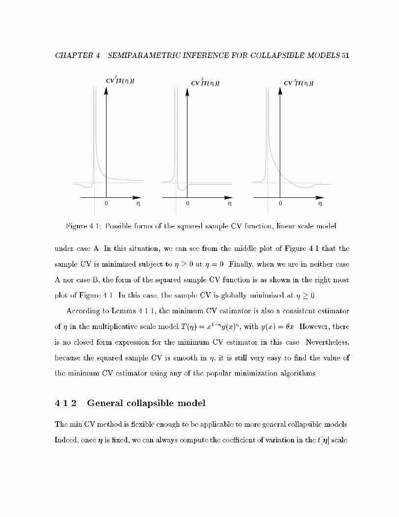
CHAPTER 4. SEMIPARAMETRIC INFERENCE FOR COLLAPSIBLE MODELS 51
CV2
CV CV2 2[T( [T( [T(η η η
η η η
)] )] )]
0 0 0
Figure 4.1: Possible forms of the squared sample CV function, linear scale model.
under case A. In this situation, we can see from the middle plot of Figure 4.1 that the
sample CV is minimized subject to � � 0 at � = 0. Finally, when we are in neither case
A nor case B, the form of the squared sample CV function is as shown in the right most
plot of Figure 4.1. In this case, the sample CV is globally minimized at � � 0.
According to Lemma 4.1.1, the minimum CV estimator is also a consistent estimator
of � in the multiplicative scale model T (�) = x1��y(x)�, with y(x) = �x. However, there
is no closed form expression for the minimum CV estimator in this case. Nevertheless,
because the squared sample CV is smooth in �, it is still very easy to �nd the value of
the minimum CV estimator using any of the popular minimization algorithms.
4.1.2 General collapsible model
The min CVmethod is exible enough to be applicable to more general collapsible models.
Indeed, once � is �xed, we can always compute the coe�cient of variation in the t[�] scale.

CHAPTER 4. SEMIPARAMETRIC INFERENCE FOR COLLAPSIBLE MODELS 52
However, it is a lot more di�cult to derive the properties of the min CV estimator when
the model at hand is not a member of the separable scale family. Nonetheless, we know
that the sample mean and variance of the ti[�]'s are consistent estimators of the true
mean and variance of T [�] for every �xed value of �1. This implies that the min CV
estimator will be consistent in every case where the true CV is uniquely minimized at
the true value of �.
4.1.3 Censored observations
The min CV method is not as tractable when some of the observations in the sample are
censored. Kordonsky and Gertsbakh (1997b) suggest a somewhat odd way of estimating
� when censored observations are present. Their method is simply a hybrid of ML and
min CV; they assume a parametric form for the survivor function, G[�;�], and they use
the following algorithm:
1. �x � = �1;
2. �nd �1 = argmax� L(�1;�);
3. compute the CV of G[�;�1];
4. repeat steps 1, 2 and 3 until the CV in step 3 is minimized
Of course, proceeding this way defeats the purpose of semiparametric estimation, i.e.
estimating � before making any strong assumption about the form of G[�]. Moreover, why
should one use ML to get estimates of some parameters of the model and then use another
method to get estimates of the other parameters? Kordonsky and Gertsbakh claim that
1Under suitable regularity conditions, such as the smoothness of E[T [�]] and Var[T [�]] in �.

CHAPTER 4. SEMIPARAMETRIC INFERENCE FOR COLLAPSIBLE MODELS 53
in the case where G[�] is the log-normal distribution, their method yields estimates of �
in the linear scale model that are very close to the ML estimates. As it turns out, it
can easily be shown that in this case, for a complete sample, Kordonsky and Gertsbakh's
hybrid method is equivalent to maximum likelihood!
So how can we estimate � semiparametrically when censoring is present using the min
CV method? Obviously, we cannot compute the usual sample mean and variance if we
do not have complete data. However, if we see the squared coe�cient of variation as a
real functional, then it is possible to de�ne a censored version of it. Let us �rst de�ne
D[0; 1] to be the set of all mappings F : IR ! [0; 1] that are cdf's. Then we can de�ne
the squared CV as a mapping CV 2 : D[0; 1]! IR+ this way:
CV 2(F ) =
R(u� R u dF (u))2 dF (u)
[Ru dF (u)]2
=
Ru2 dF (u)
[Ru dF (u)]2
� 1: (4.7)
Using this approach, we can de�ne the minimum CV estimator in an alternative, more
general manner:
De�nition 4.2 Let ti[�] = �[P
i(x
i);�]; i = 1; 2; : : : ; n be the values of the observed
sample translated in the new scale, which we denote T [�] for some �xed �. Let F̂� be the
estimated cdf obtained from t1[�]; : : : ; tn[�]. We de�ne the min CV estimator to be the
value of � that minimizes CV 2(F̂�) as de�ned in equation (4.7).
If there is no censoring, we can use the usual empirical cdf for F̂ and this yields the usual
min CV estimator, as de�ned by Kordonsky and Gertsbakh. However, when censoring is
present, we have to be careful. If the largest time in the sample ti[�]; i = 1; 2; : : : ; n is a
failure time, we can de�ne F̂� to be the usual product-limit estimator and then compute
the min CV estimator according to De�nition 4.2. When the largest value of the sample

CHAPTER 4. SEMIPARAMETRIC INFERENCE FOR COLLAPSIBLE MODELS 54
is a censoring time, we need to de�ne the estimator of F� slightly di�erently. Let tmax[�]
be the largest observed failure time in the sample. We then de�ne an estimator of F� in
this manner:
F̂�(t) =
8>><>>:F̂ PL
� (t); 0 � t � tmax[�];
1 � expf��̂tg; t > tmax[�];; (4.8)
where
�̂ =� ln[1� F̂ PL
� (tmax[�])]
tmax[�];
and F̂ PL
� is the usual product-limit estimator of F�. One can see that we are just assuming
that the tail of the distribution beyond tmax[�] follows an exponential distribution. This
will usually give a good estimate of the �rst two moments of F�, hence we can use
estimator (4.8) in De�nition 4.2. Unfortunately, there is no closed form solution for
�̂ in this case and the numerical optimization is actually quite challenging, unless � is
unidimensional, in which case the usual numerical methods, such as golden section search
(see Press et al. (1992, Section 10.1)), seem to work relatively well.
The behavior of the estimators thereby obtained still needs to be studied. Indeed, the
\empirical" cdf (4.8) in this case depends on the parameter to be estimated. Moreover,
when the largest observation in the t[�] scale is censored, the tail of the \empirical" cdf is
approximated by the tail of an exponential distribution. Needless to say, the derivation
of the asymptotic properties of this generalized minimum CV estimator represents quite
a challenging problem.
4.1.4 Variance estimate
Despite its simplicity, it is very di�cult to compute a good variance estimate for the
min CV estimator. Even in the linear scale case, where a closed form expression for this

CHAPTER 4. SEMIPARAMETRIC INFERENCE FOR COLLAPSIBLE MODELS 55
estimator is available, the variance that must be calculated is the variance of a ratio of
products of correlated sums of random variables. Moreover, the min CV estimator cannot
be expressed as an M-estimator, or a U-statistic or any type of functional for which the
asymptotics have already been worked out.
Since the minimum CV method is based on the joint distribution of the real times
and the usage paths, resampling based on this empirical joint distribution should at
least give an idea of the precision of the estimate. More precisely, suppose we observe
(x1; y1); : : : ; (xn; yn) and that we estimate � in T (�) via minimum CV. Then the variance
estimate obtained via the following bootstrap algorithm is a good approximation of the
true variance of the estimator:
1. For b = 1 to B:
(a) sample n pairs with replacement from the original pairs (x1; y1); : : : ; (xn; yn);
(b) compute the minimum CV estimator of � based on this new sample and call
this estimate �̂b;
2. The variance estimate of �̂ is then given by
BXb=1
��̂b� �̂
�2B � 1
;
where �̂ =P
B
b=1 �̂b=B.
According to Efron and Tibshirani (1993), a value of B around 200 is usually su�cient
for variance estimates.
The algorithm above also gives a good approximation of the distribution of the esti-
mator. We used the percentile bootstrap algorithm (see Efron and Tibshirani (1993) for a

CHAPTER 4. SEMIPARAMETRIC INFERENCE FOR COLLAPSIBLE MODELS 56
description of this method) and the minimum CV to derive approximate 95% con�dence
intervals for the time scale parameter for the linear scale model. We used a value of
B = 1000, as recommended by Efron and Tibshirani (1993). The results are given in
Table 4.30 in Section 4.4.4.
4.2 Quasi-likelihood
When no censoring is present, we can use unbiased linear estimating equations (EE's) to
estimate � in model (4.1). These EE's show good robustness properties and are relatively
simple to implement. Moreover, some EE's are fully e�cient for certain forms of G.
Suppose that we have a complete sample of real times at failure, xi, along with the
corresponding usage paths, Pi, for i = 1; : : : ; n. In this section, we consider EE's of the
formnXi
wi;j
�h(x
i)� E[h(X
i)jP
i;�; �]
�= 0; j = 1; 2; : : : ; p+ 1; (4.9)
where p = dim(�), h(�) is a strictly monotonic function and wijis some weight. In
this chapter, we use a parameterization with the minimal number of parameters, p, in
the ITS (see comment on parameterization following equation (3.10) in Section 3.3.1).
This means that � does not contain a scale parameter; this scale parameter is accounted
for in the value of the parameter �. There is an extensive literature on such EE's (see
Godambe and Thompson (1989)). For any �xed function h(�), it is possible to derive
optimal weights wij's. Unfortunately, the optimal h(�) function will depend on the form
of G in (4.1). We will therefore limit our investigation to a few �xed choices of h(�).
CHAPTER 4. SEMIPARAMETRIC INFERENCE FOR COLLAPSIBLE MODELS 57
4.2.1 Separable scale model
Let us now assume that tPi(xi;�) = u(xi)v(�
i;�) and let z
i= u(x
i). We wish to estimate
� using EE's of the form
nXi=1
wi;j
�h(z
i)� E[h(Z
i)j�
i;�; �]
�= 0; j = 1; 2 : : : ; p+ 1: (4.10)
Note that even though dim(�) = p, we need p + 1 EE's. This is due to the fact that
the conditional expectation involved in (4.10) will be a function of an extra unknown
parameter, namely the moment � = � R h(u) dG(u). We also must point out that care
is needed in the parameterization here; EE's (4.10) are scale invariant, and therefore one
must make sure that the parameters � will not be confounded with a scale parameter.
We �rst derive the best EE's for h(u) = u. First, we see that
�i(�; �
T) = E[Z
ij�
i;�; �] = �
T=v(�
i;�);
where �T= � R u dG(u), i.e. the �rst moment of distribution G. We also observe that
�2i
(�; �T; �2
T
) = Var[Zij�
i;�; �] = �2
T
=v(�i;�)2;
where �2T
= � R (u� �T)2 dG(u), i.e. the variance of distribution G. We then notice that
�2i(�; �
T; �2
T) = ��
i(�; �
T)2, where � = �2
T=�2
T. Applying well known quasi-likelihood
results (see McCullagh and Nelder (1989), for example), we obtain the following optimal
EE's:
nXi=1
@v(�i;�)
@�j
�zi� �
T
v(�i;�)
�= 0; j = 1; 2; : : : ; p (4.11)

CHAPTER 4. SEMIPARAMETRIC INFERENCE FOR COLLAPSIBLE MODELS 58
nXi=1
v(�i;�)
�zi� �
T
v(�i;�)
�= 0: (4.12)
Solving (4.12) for any �xed � yields �̂T(�) = t[�], the sample mean of the z
iv(�
i;�)
values. The system of EE's in � left to solve is thus
nXi=1
@v(�i;�)
@�j
�zi� t[�]
v(�i;�)
�= 0; j = 1; 2; : : : ; p (4.13)
or, equivalently,nXi=1
@ ln v(�i;�)
@�j
�ti[�]� t[�]
�= 0; j = 1; 2; : : : ; p; (4.14)
where ti[�] = z
iv(�
i;�). As it turns out, EE (4.14) is the ML equation for � when G[�;�]
is the exponential survivor function.
Repeating the same procedure for h(zi) = ln z
i, we obtain the following optimal EE's:
nXi=1
@ ln v(�i;�)
@�j
�ln z
i� �lnT + ln v(�
i;�)
�= 0; j = 1; 2; : : : ; p (4.15)
nXi=1
�ln z
i� �lnT + ln v(�
i;�)
�= 0; (4.16)
where �lnT = � R ln u dG(u). Then solving (4.12) for �lnT and substituting in (4.15)
yieldsnXi=1
@ ln v(�i;�)
@�j
�ln t
i[�]� ln t[�]
�= 0; j = 1; 2 : : : ; p; (4.17)
where ln ti[�] = ln z
i+ ln v(�
i;�) and ln t[�] is the sample mean of the ln t
i[�]'s. This
time, EE (4.17) is the ML equation for � when G is the lognormal survivor function.
Finally, another form for h(�) is h(zi) = z�
i, for some �xed � > 0. Popular choices of
CHAPTER 4. SEMIPARAMETRIC INFERENCE FOR COLLAPSIBLE MODELS 59
� in regression are � = 1=2 or � = 2. Going through the same calculations again yields
nXi=1
@v(�i;�)
@�j
v(�i;�)��1
�z�i� �
T�
v(�i;�)�
�= 0; j = 1; 2; : : : ; p (4.18)
nXi=1
v(�i;�)�
�z�i
� �T�
v(�i;�)�
�= 0; (4.19)
where �T� = � R u� dG(u). The next step gives
nXi=1
@ ln v(�i;�)
@�j
�ti[�]� � t[�]�
�= 0; j = 1; 2 : : : ; p; (4.20)
where ti[�]� = z�
i
v(�i;�)� and t[�]� is the sample mean of the t
i[�]�'s. We can show
that EE (4.20) is the ML equation for � when G is the survivor function of a Weibull
distribution with shape parameter known and equal to �. This should not come as a
surprise; when T is Weibull with shape �, then T � is exponential, and we have already
seen that EE (4.14) is the ML equation for � when G is the exponential survivor function.
It is worth pointing out that for all our choices of the function h(�), the EE's for �are of the form
nXi=1
@ ln v(�i;�)
@�
�h(t
i[�])� h(t[�])
�= 0: (4.21)
This is not necessarily true for all strictly monotone functions h(�), though.One very interesting interpretation of (4.21) is that we are looking for a value of
� such that the sample covariance between @ ln v(�;�)=@� and h(T [�]) is zero. This
means that the quasi-likelihood EE's are consistent with the ITS de�nition in that they
are looking for a value of � such that the failure times in the ITS are orthogonal to some
path feature.
We can easily derive the asymptotic distribution of �̂ obtained by solving the EE's

CHAPTER 4. SEMIPARAMETRIC INFERENCE FOR COLLAPSIBLE MODELS 60
described by (4.21). We let
A(�; �h(T ))r;s =
1
n
nXi=1
1
g(�i)
@�
i
@�r
! @�
i
@�s
!; r; s = 1; 2; : : : ; p + 1;
where �i= E[h(Z
i)j�
i;�; �
h(T )] and g(�) is such that Var[h(Zi)j�
i;�; �
h(T )] = �g(�i) for
some real number �. (We can show that � = � R (h(u) � �h(T ))
2 dG(u)=�2h(T ) when
h(u) = u� and � > 0, and � = � R (h(u)� �h(T ))
2 dG(u) when h(u) = ln u.)
The asymptotic distribution of��̂
�̂h(T )
�is then given by
pn
" �̂
�̂h(T )
!�
�
�h(T )
!#d! N
h0; �A�1(�; �
h(T ))i: (4.22)
Let us now apply these results to the linear and multiplicative scale models in the
case with a single usage measure of the form yi(x) = �
ix. With the linear scale model,
we have that tP(x; �) = (1 � �)x + �y(x) = x(1 � � + ��). We thus get zi= x
iand
v(�i; �) = (1� � + ��
i). Substituting these quantities in (4.21) yields
nXi=1
�i� 1
1� � + ��i
�h(t
i[�])� h(t[�])
�= 0; (4.23)
where h(ti[�]) = h(x
i(1 � � + ��
i)) and h(t[�]) =
Pih(t
i[�])=n.
We can also use (4.22) to derive the asymptotic variance of �̂, the root of (4.23).
Case h(u) = u�: In this case, we get that
asvar[�̂] =�
ndVar h ��11��+��
i; (4.24)
where � = � R (u���T�)2 dG(u)=�2
T� is the squared CV of T � and dVar denotes the
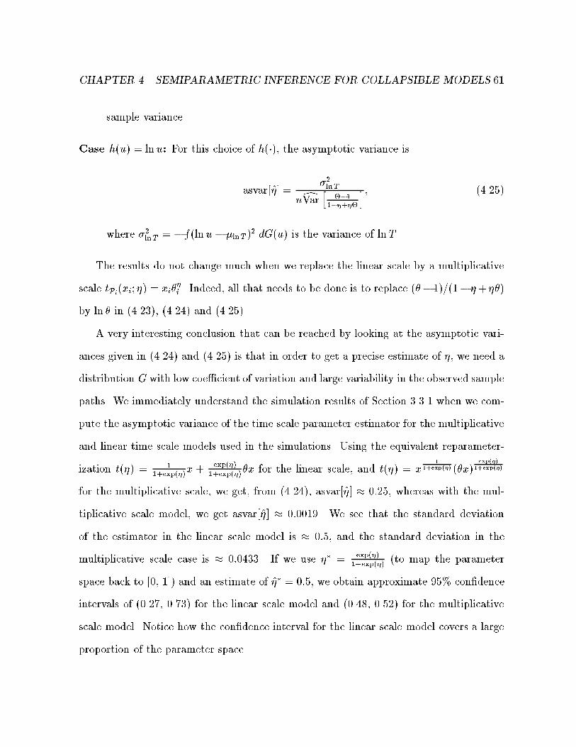
CHAPTER 4. SEMIPARAMETRIC INFERENCE FOR COLLAPSIBLE MODELS 61
sample variance.
Case h(u) = ln u: For this choice of h(�), the asymptotic variance is
asvar[�̂] =�2lnT
ndVar h ��11��+��
i; (4.25)
where �2lnT = � R (ln u� �lnT )2 dG(u) is the variance of ln T .
The results do not change much when we replace the linear scale by a multiplicative
scale tPi(xi; �) = xi��
i. Indeed, all that needs to be done is to replace (�� 1)=(1� �+ ��)
by ln � in (4.23), (4.24) and (4.25).
A very interesting conclusion that can be reached by looking at the asymptotic vari-
ances given in (4.24) and (4.25) is that in order to get a precise estimate of �, we need a
distribution G with low coe�cient of variation and large variability in the observed sample
paths. We immediately understand the simulation results of Section 3.3.1 when we com-
pute the asymptotic variance of the time scale parameter estimator for the multiplicative
and linear time scale models used in the simulations. Using the equivalent reparameter-
ization t(�) = 11+exp(�)
x + exp(�)
1+exp(�)�x for the linear scale, and t(�) = x
11+exp(�) (�x)
exp(�)
1+exp(�)
for the multiplicative scale, we get, from (4.24), asvar[�̂] � 0:25, whereas with the mul-
tiplicative scale model, we get asvar[�̂] � 0:0019. We see that the standard deviation
of the estimator in the linear scale model is � 0:5, and the standard deviation in the
multiplicative scale case is � 0:0433. If we use �� = exp(�)
1+exp(�)(to map the parameter
space back to [0, 1]) and an estimate of �̂� = 0:5, we obtain approximate 95% con�dence
intervals of (0.27, 0.73) for the linear scale model and (0.48, 0.52) for the multiplicative
scale model. Notice how the con�dence interval for the linear scale model covers a large
proportion of the parameter space.

CHAPTER 4. SEMIPARAMETRIC INFERENCE FOR COLLAPSIBLE MODELS 62
4.2.2 General collapsible model
We can still derive EE's for � when the ITS is not of the separable form. However, in
this more general case, we do not necessarily have Var[h(Xi)jP
i] = �g(E[h(X
i)jP
i]), so
we cannot use the quasi-likelihood EE's. We can nevertheless use linear EE's of the form
(4.9) and derive weights wijthat are optimal in some sense. However, the moments of X,
the real time at failure, given a usage path P may be di�cult to compute in practice. For
this reason, semiparametric methods that do not require the calculation of conditional
moments, such as min CV or rank based methods, seem to be more appropriate for more
complicated collapsible models.
4.2.3 Censored observations
As was the case with the min CV method, quasi-likelihood and other methods based on
comparing observations with sample moments are di�cult to generalize so that they can
handle censoring. Using an EM-type algorithm and replacing the censoring times, say x�i,
with values of the form E[XijX
i> x�
i; �
i;�; �] would not work here as we do not want to
assume a parametric form for the survivor function G and, hence, cannot compute this
last conditional expectation. Once again, we recommend the use of rank based methods
when censoring is present.
4.3 Rank based methods
Semiparametric inference methods based on ranks are quite popular in survival analysis.
These methods can easily be generalized to handle censoring, they are usually close to
e�cient and they are quite robust. In this section, we follow the methodology of Lin and

CHAPTER 4. SEMIPARAMETRIC INFERENCE FOR COLLAPSIBLE MODELS 63
Ying (1995) in order to derive a rank based method for estimating semiparametrically
the time scale parameter in a collapsible model.
4.3.1 General collapsible model
We �rst consider a rank based method for a general collapsible model with an ITS of the
form tPi(x;�). We now write the log likelihood under some fully speci�ed (but unknown)
distribution G using the counting process notation of Andersen et al. (1993):
l(�) =nXi=1
Z1
0
��ln �[tPi(x;�)] + ln t0Pi(x;�)
�dN
i(x) (4.26)
�Yi(x)�[tPi(x;�)]t
0
Pi(x;�)dx
�;
where �[u] is the hazard function corresponding to G(u), Ni(u) is a counting process
taking value 0 if u < Xiand 1 if u � X
i, Y
i(u) is 1 if individual i is at risk of failing
at real time u (i.e., individual i is still alive and uncensored at the instant before u), 0
otherwise, and t0Pi(x;�) = dtPi(x;�)=dx. Assuming that the usual regularity conditions
hold, we can take the derivative with respect to � under the integral sign and obtain the
following score function:
U(�) =nXi=1
Z1
0
( �0[tPi(x;�)]
�[tPi(x;�)]
@tPi(x;�)
@�+@t0Pi(x;�)=@�
t0Pi(x;�)
!dN
i(x) (4.27)
�Yi(x)
�0(tPi(x;�)]
@tPi(x;�)
@�t0Pi(x;�) + �[tPi(x;�)]
@t0Pi(x;�)
@�
!dx
):
Following Robins and Tsiatis (1992) and Lin and Ying (1995), we now make the as-
sumption that �0[u] = 0. This will yield maximum e�ciency when G is the exponential

CHAPTER 4. SEMIPARAMETRIC INFERENCE FOR COLLAPSIBLE MODELS 64
distribution. The score (4.27) then becomes
U(�) =nXi=1
Z1
0
(@t0Pi(x;�)=@�
t0Pi(x;�)dN
i(x)� Y
i(x)�[tPi(x;�)]
@t0Pi(x;�)
@�dx
)
=nXi=1
Z1
0
@ ln t0Pi(x;�)
@�
�dN
i(x)� Y
i(x)�[tPi(x;�)]t
0
Pi(x;�)dx
�
=nXi=1
Z1
0
@ ln t0Pi(x;�)
@�
�dN
i(x)� Y
i(x) d�[tPi(x;�)]
�; (4.28)
where �[u] =Ru
0 �[t]dt = � lnG[u] is the cumulative hazard function corresponding to G.
What Lin and Ying (1995) do at this stage is replace � by a \good" nonparametric
estimator of it. This is straightforward once the value of � has been �xed; all we need to
do is calculate the failure and censoring times in scale tP(�;�) and then estimate � using
the Nelson-Aalen estimator. In more precise terms, let
fNi(t;�) =
8>><>>:0; if t < tPi(Xi
;�)
1; if t � tPi(Xi;�)
eYi(t;�) =
8>><>>:1; if individual i is at risk of failing at time t in scale tP(�;�)0; otherwisee�[t;�] = value of Nelson-Aalen estimator in scale tP(�;�) at time t.
Substituting these values in (4.28) yields
eU (�) = nXi=1
Z1
0
@ ln t0Pi(x;�)
@�
�����x=x�1[t;�;Pi]
�dfN
i(t;�)� eY
i(t;�) de�[t;�]�; (4.29)
where x�1[t;�;Pi] is the value of x such that tPi(x;�) = t. This score functionis an
unbiased linear rank estimating equation. Indeed, we can re-write (4.29) in the following
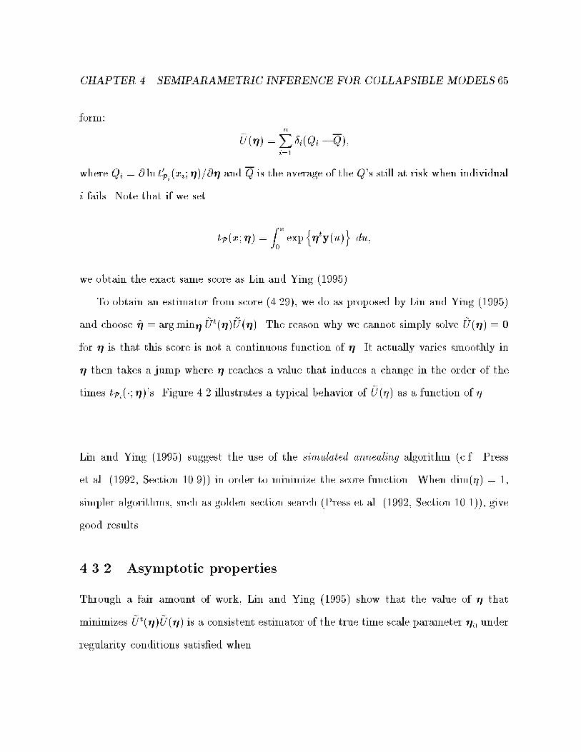
CHAPTER 4. SEMIPARAMETRIC INFERENCE FOR COLLAPSIBLE MODELS 65
form:
eU (�) = nXi=1
�i(Q
i�Q);
where Qi= @ ln t0
Pi(x
i;�)=@� and Q is the average of the Q's still at risk when individual
i fails. Note that if we set
tP(x;�) =Z
x
0exp
n�ty(u)
odu;
we obtain the exact same score as Lin and Ying (1995).
To obtain an estimator from score (4.29), we do as proposed by Lin and Ying (1995)
and choose �̂ = arg min� eU t(�) eU (�). The reason why we cannot simply solve eU(�) = 0
for � is that this score is not a continuous function of �. It actually varies smoothly in
� then takes a jump where � reaches a value that induces a change in the order of the
times tPi(�;�)'s. Figure 4.2 illustrates a typical behavior of eU(�) as a function of �.
Lin and Ying (1995) suggest the use of the simulated annealing algorithm (c.f. Press
et al. (1992, Section 10.9)) in order to minimize the score function. When dim(�) = 1,
simpler algorithms, such as golden section search (Press et al. (1992, Section 10.1)), give
good results.
4.3.2 Asymptotic properties
Through a fair amount of work, Lin and Ying (1995) show that the value of � that
minimizes eU t(�) eU(�) is a consistent estimator of the true time scale parameter �0 under
regularity conditions satis�ed when
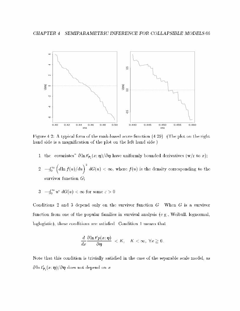
CHAPTER 4. SEMIPARAMETRIC INFERENCE FOR COLLAPSIBLE MODELS 66
eta
U(eta
)
0.40 0.42 0.44 0.46 0.48 0.50
-6-4
-20
24
6
eta
U(eta
)0.440 0.445 0.450 0.455 0.460
-0.5
0.00.5
Figure 4.2: A typical form of the rank-based score function (4.29). (The plot on the righthand side is a magni�cation of the plot on the left hand side.)
1. the \covariates" @ ln t0Pi(x;�)=@� have uniformly bounded derivatives (w/r to x);
2. � R10 �d ln f(u)=du
�2
dG(u) < 1, where f(u) is the density corresponding to the
survivor function G;
3. � R10 u" dG(u) <1 for some " > 0.
Conditions 2 and 3 depend only on the survivor function G. When G is a survivor
function from one of the popular families in survival analysis (e.g., Weibull, lognormal,
loglogistic), these conditions are satis�ed. Condition 1 means that
����� ddx @ ln t0p(x;�)
@�
����� < K; K <1; 8x � 0:
Note that this condition is trivially satis�ed in the case of the separable scale model, as
@ ln t0Pi(x;�)=@� does not depend on x.

CHAPTER 4. SEMIPARAMETRIC INFERENCE FOR COLLAPSIBLE MODELS 67
Under conditions 1-3, Lin and Ying (1995) show that the minimizer of eU t(�) eU(�) isstrongly consistent and that
(�) = eU t(�)V �1(�̂) eU(�) asymp.� �2p; (4.30)
where �2p
represents a chi-squared distribution on p = dim(�) degrees of freedom and
n�1V (�) is an estimate of the variance of eU(�) with
V (�) =nXi=1
Z1
0
264Pn
j=1eYj(t;�)Z
j(t;�)2P
n
j=1eYj(t;�)
�0@Pn
j=1eYj(t;�)Z
j(t;�)P
n
j=1eYj(t;�)
1A2375 dfN
i(t;�);
(4.31)
where
Zj(t;�) =
@ ln t0Pj(x;�)
@�
�����x=x�1(t;�;Pj)
and, for some column-vector z, z2 denotes the outer product zzt.
We can thus use the quadratic form (4.30) to derive a (1-�)-level con�dence region for
�: f� : (�) < �2p:1��g, where �2
p:1�� is the (1-�)th quantile of a chi-squared distribution
on p degrees of freedom. Asymptotically equivalent con�dence regions can be built using
f� : e (�) < �2p:1��g, where
e (�) = eU t(�)V �1(�) eU(�): (4.32)
For large samples, quadratic forms (4.30) and (4.32) are equivalent. However, they may
yield di�erent con�dence regions for moderate size samples in some situations. In the
simulations study of Section 4.4, we consider both types of con�dence regions and give
guidelines as to which type to use for moderate size samples.

CHAPTER 4. SEMIPARAMETRIC INFERENCE FOR COLLAPSIBLE MODELS 68
4.3.3 Separable scale model
We now apply the results derived above to the separable scale model. In this case, we
have that
@ ln t0Pi(x;�)
@�=@ ln v(�
i;�)
@�:
We then substitute this quantity into (4.28) to obtain
U(�) =nXi=1
Z1
0
@ ln v(�i;�)
@�
�dN
i(x)� Y
i(x) d�[u(x)(�
i;�)]
�: (4.33)
Replacing � in (4.33) by the Nelson-Aalen estimator computed in scale tP(�;�) then givesthe score
eU (�) = nXi=1
Z1
0
@ ln v(�i;�)
@�
�dfN
i(t;�)� eY
i(t;�) de�[t;�]�: (4.34)
As we can see, this score is somewhat close to the score (4.21), obtained through quasi-
likelihood. In the special case where there is no censoring, score (4.34) simpli�es to
eU (�) = nXi=1
@ ln v(�(i);�)
@�
�1�
�1
n+
1
n� 1+ � � � + 1
n� i+ 1
��; (4.35)
where �(i) is the path parameter corresponding to the ith smallest failure time under
scale tP(�;�). Note that we would have obtained the exact same score function had we
wanted to test � = 0 in ln Ti[�] = � + �t@ ln v(�
i;�)=@� + "
i, where "
i's are i.i.d. and
� is �xed, using rank regression and exponential scores (see Cox and Hinkley (1974) or
Kalb eisch and Prentice (1980)). This method is thus consistent with our de�nition of
ITS, i.e. we are looking for a value of � such that the failure times in the scale tP(�;�)are \as unrelated as possible" to some function of the usage path parameter �.

CHAPTER 4. SEMIPARAMETRIC INFERENCE FOR COLLAPSIBLE MODELS 69
To illustrate this method, let us see what the score and variance estimate look like in
the case of the linear scale model. Substituting v(�;�) = (1� � + ��) in (4.33) gives
eU (�) = nXi=1
Z1
0
�i� 1
1 � � + ��i
�dfN
i(t; �)� eY
i(t; �) de�[t; �]�: (4.36)
We can then use the fact that eU2(�)= eV (�) is approximately chi-squared on one degree of
freedom to derive an approximate (1� �)100% con�dence interval for �:
n� : eU2(�)=V (�̂) � �2
1;1��
o; (4.37)
where �21;1�� is the (1 � �)th quantile of a chi-squared distribution on one degree of
freedom and V (�̂) is obtained by substituting Zj(t;�) = (�
j� 1)=(1� � + ��
j) in (4.31).
4.3.4 Application of the method
This rank based method can be used in most frameworks as long as we have enough data
to compute the score function. When @ ln t0P(x;�)=@� does not depend on x, such as
in the separable scale model, we only need to observe the real times of failure/censoring
along with the path parameter values, �. Unfortunately, when @ ln t0P(x;�)=@� does
depend on x, we need more information. In that case, for each unit we need to know the
values of the usage measures and their derivative with respect to x at all the di�erent real
times at failure present in the sample. In addition, for units that get censored, we need
to know the value of their usage measures at censoring. This problem is not new though;
it is actually the same problem as with partial likelihood inference for the proportional
hazards model when time-varying covariates are present.
All the semiparametric inference methods mentioned in this chapter yield consistent

CHAPTER 4. SEMIPARAMETRIC INFERENCE FOR COLLAPSIBLE MODELS 70
estimators. However, the variance of these estimators (and thus, probably, their e�-
ciency) tends to vary with the choice of the survivor function G and the distribution of
the observed usage paths. It would therefore be of interest to know which methods are
more e�cient for a given time scale model, and this for samples of moderate size. In the
next section, we compare the e�ciency of the semiparametric methods outlined in this
chapter through simulation. We also use these simulations to assess the accuracy of the
various variance estimates and/or con�dence intervals.
4.4 Simulation study
Because of the complexity of the models at hand, we compare the e�ciency of the var-
ious estimators proposed in this chapter through a simulation study. We also use the
simulation results to assess the accuracy of the variance estimators and of the con�dence
intervals.
In Section 4.4.1, we generate data from the linear scale model. We use the multi-
plicative scale model in Section 4.4.2 and a collapsible model that is not of the separable
form and for which the covariates vary in time in Section 4.4.3. For each sample simu-
lated, we compute the ML, rank (minimizer of the square of (4.34), denoted \Rank"),
quasi-likelihood (root of (4.14), denoted \Quasi-like.") and minimum CV (Min CV) esti-
mators. For the samples obtained from the multiplicative scale model, we also compute
the popular ordinary least squares (OLS) estimator of � based on the logarithmic time
scale log T [�] = log x+ � log � (see Lawless (1982), for example).

CHAPTER 4. SEMIPARAMETRIC INFERENCE FOR COLLAPSIBLE MODELS 71
4.4.1 Linear scale model
We generated data from the linear scale model
Pr [X > xj�] = G[(1 � �)x+ ��x]: (4.38)
We used a value of � = 0:5, four di�erent distributions for G and two distributions for
the usage paths, �. We simulated 2000 samples of size 102 in each batch.
The results of the simulations were in agreement with the theoretical results of the
previous sections; with the linear scale model, large variability in the observed values
of � and a more compact distribution G lead to much more precise inference. We also
obtain that all the studied estimators have small bias, but their relative e�ciencies vary
with changes in G.
Batch 1
We simulated Batch 1 from the linear scale model t�(x) = (1 � 0:5)x+ 0:5�x with
1. G(u) = exp���
u
1000
�3�;
2. atan(�) � Uniform(0; �=2).
The �fth, �ftieth and ninety-�fth percentiles of the distribution G are t0:05 = 371:6,
t0:50 = 885:0 and t0:95 = 1441:6. The same percentiles for the distribution of the slope
parameter are �0:05 = 0:0787, �0:50 = 1:0 and �0:95 = 12:71. To get more insight on
whether or not we can estimate � accurately and on the plausibility of this scenario, we
can look at the percentiles of real time at failure, x, conditional on the path parameter,
�, for a few values of �. These values are summarized in Table 4.1 and on Figure 4.3

CHAPTER 4. SEMIPARAMETRIC INFERENCE FOR COLLAPSIBLE MODELS 72
� = 0:25 � = 0:50 � = 0:75
�0:05 �0:50 �0:95 �0:05 �0:50 �0:95 �0:05 �0:50 �0:95(0.0787) (1.0) (12.71) (0.0787) (1.0) (12.71) (0.0787) (1.0) (12.71)
x0:05 688.9 371.6 54.22 482.7 371.6 94.63 1203 371.6 37.99
x0:50 1150 885.0 225.4 1641 885.0 129.1 2864 885.0 90.49
x0:95 1873 1441 367.1 2673 1441 210.4 4665 1441 147.4
Table 4.1: Percentiles of real time at failure given usage path, linear scale model, Batch
1.
As we can see, di�erent values of � yield fairly di�erent conditional distributions for
real time at failure given the usage path. We should therefore be able to estimate the
value of � accurately from this model. Table 4.2 con�rms this last statement. If we look
at the standard deviations obtained from the simulations (Table 4.2, 2nd column), we
see that roughly 95% of the times, the estimates will be in the range (0.43, 0.57), which
is fairly close to the true value, 0.5. We also notice the extremely high e�ciency of the
rank and minimum CV estimators relative to ML.
Estimator Average Standard Deviation Relative E�ciency
ML 0.5003 0.03199 100.0%Rank 0.5003 0.03238 97.6%
Quasi-like. 0.5004 0.03544 81.5%Min CV 0.5003 0.03202 99.8%
Table 4.2: Simulation results, linear scale model, Batch 1.
Batch 2
We simulated Batch 2 from the linear scale model t�(x) = (1 � 0:5)x+ 0:5�x with
1. G(u) = expn� u
1000
o;

CHAPTER 4. SEMIPARAMETRIC INFERENCE FOR COLLAPSIBLE MODELS 73
������
������
����
������
������
����
��������
���
���
������
������
����
������������������������������������������������������������������������������������������������������������������������������������������������������������������������������������������������������������������������������������������������������������������������������������������������������������������������������������������������������������������������������������������������������������������������������������������������������������������������������������������������������������������������������������������������������������������������������������������������������������������������������������������������������������������������������������������������������������������������������������������������������������������������������������������������������������������������������������������������������������������������������������������������������������������������������������������������������������������������������������������������������������������������������������������������������������������������������������������������������������������������������������������������������������������������������������������������������������������������������������������������������������������������������������������������������������������������������������������������������������������������������������������������������������������������������������������������������������������������������������������������������������������������������������������������������������������������������������������������������������������������������������������������������������������������������������������������������������������������������������������������������������������������������������������������������������������������������������������������������������������������������������������������������������������������������������������������������������������������������������������������������������������������������������������������������������������������������������������������������������������������������������������������������������������������������������������������������������������������������������������������������������������
������������������������������������������������������������������������������������������������������������������������������������������������������������������������������������������������������������������������������������������������������������������������������������������������������������������������������������������������������������������������������������������������������������������������������������������������������������������������������������������������������������������������������������������������������������������������������������������������������������������������������������������������������������������������������������������������������������������������������������������������������������������������������������������������������������������������������������������������������������������������������������������������������������������������������������������������������������������������������������������������������������������������������������������������������������������������������������������������������������������������������������������������������������������������������������������������������������������������������������������������������������������������������������������������������������������������������������������������������������������������������������������������������������������������������������������������������������������������������������������������������������������������������������������������������������������������������������������������������������������������������������������������������������������������������������������������������������������������������������������������������������������������������������������������������������������������������������������������������������������������������������������������������������������������������������������������������������������������������������������������������������������������������������������������������������������������������������������������������������������������������������������������������������������������������������������������������������������������������������������������������������������
y(x)
xt t t
θ
= = =
���
���
=
0.0787θ=
θ=
η=0.5
x= 1441.6
x=
x=
x=
x=
x=
x=
x=x=
482.71641
2673
371.6
885.0
94.63
129.1
210.4
743.2 1770 2882
12.71
1.0
Figure 4.3: Percentiles of real time at failure given usage path, linear scale model, Batch1.
2. atan(�) � Uniform(0; �=2).
The distribution for the usage paths is the same as in Batch 1. However, the distribution
G has a shape parameter of value less than in Batch 1. This means that the CV of G
is smaller and we therefore should observe less precision in the inference procedures. In
fact, if one carries out the calculations, one �nds that the CV of G in Batch 2 is about
2.75 times the CV of G in Batch 1.
To get a better idea of how this model is di�erent from the model used in Batch 1,
we compute the same conditional quantiles of real time at failure as in Table 4.1.
Table 4.4 summarizes the results. As expected, the validity of all the estimators was
still good, but the variability increased. The simulation standard deviations were close
to 2.75 times as large as they were for Batch 1, which is what we expected.

CHAPTER 4. SEMIPARAMETRIC INFERENCE FOR COLLAPSIBLE MODELS 74
� = 0:25 � = 0:50 � = 0:75
�0:05 �0:50 �0:95 �0:05 �0:50 �0:95 �0:05 �0:50 �0:95(0.0787) (1.0) (12.71) (0.0787) (1.0) (12.71) (0.0787) (1.0) (12.71)
x0:05 66.64 51.29 13.06 95.10 51.29 7.485 166.0 51.29 5.245
x0:50 900.6 693.1 173.5 1285 693.1 101.1 2243 693.1 70.88
x0:95 3892 2996 762.9 5554 2996 437.1 9694 2996 306.3
Table 4.3: Percentiles of real time at failure given usage path, linear scale model, Batch
2.
Estimator Average Standard Deviation Relative E�ciency
Quasi-like. (ML) 0.5007 0.0931160 100%Rank 0.5007 0.09431 97.5%
Min CV 0.4993 0.1171 63.3%
Table 4.4: Simulation results, linear scale model, Batch 2.
Batch 3
We simulated Batch 3 from the linear scale model t�(x) = (1 � 0:5)x+ 0:5�x with
1. G(u) = exp
���
u
1000
�3�;
2. ln � � N(2:37; 0:572).
The distribution G is the same as in Batch 1, but this time the usage path distribution
is clustered around � = 11 rather than uniform over the positive quadrant. We therefore
expect our inferences with the linear scale model to be highly unprecise.
We notice that the three conditional distributions of x given � in Table 4.5 do not
vary as much in �. We can thus expect more variability in the estimates of �. This is
con�rmed in Table 4.6. Except for the ML estimator, all the other estimators had a

CHAPTER 4. SEMIPARAMETRIC INFERENCE FOR COLLAPSIBLE MODELS 75
� = 0:25 � = 0:50 � = 0:75
�0:05 �0:50 �0:95 �0:05 �0:50 �0:95 �0:05 �0:50 �0:95(4.121) (10.70) (27.77) (4.121) (10.70) (27.77) (4.121) (10.70) (27.77)
x0:05 208.7 108.5 48.30 145.1 63.53 25.83 111.2 44.91 17.63
x0:50 497.2 258.4 115.0 345.7 151.3 61.52 264.9 107.0 41.99
x0:95 809.8 421.0 187.4 563.1 246.5 100.2 431.6 174.2 68.39
Table 4.5: Percentiles of real time at failure given usage path, linear scale model, Batch
3.
probability mass at �̂ = 1:0, the boundary of the parameter space. This makes e�ciency
comparisons by taking the ratio of the variances somewhat futile.
Estimator Average Standard Deviation Mean Squared Error
ML 0.5270 0.1827 0.03410
Rank 0.8071 0.2083 0.1377
Quasi-like. 0.5375 0.1971 0.04026Min CV 0.5278 0.1839 0.03461
Table 4.6: Simulation results, linear scale model, Batch 3.
As we can see in Table 4.6, the rank estimator seems to have substantial bias. This
is due to the fact that the estimator yielded a value of �̂ = 1 for a large proportion of
the samples, i.e. it identi�ed Y as the ITS. Figure 4.4 illustrates the behavior of the
rank based estimator in both Batch 1 and Batch 3. As was the case with Batch 1, the
minimum CV estimator was again very close to the ML estimator in this case. This
does not mean that the minimum CV estimator yields good results, however. A quick
look at the standard deviations of Table 4.6 clearly shows that the estimators were all
over the parameter space and did not zero in on 0.5 with any good precision. The same
observations are also true for Batches 4, 7 and 8.

CHAPTER 4. SEMIPARAMETRIC INFERENCE FOR COLLAPSIBLE MODELS 76
0.3 0.4 0.5 0.6 0.7 0.8
01
23
4atan(Theta)~U(0,PI/2)
T=0.5X+0.5Y~Weibull(3,1000)estimate
0.4 0.5 0.6 0.7 0.8 0.9 1.00
24
68
10
log(Theta)~N(2.37,0.58)
T=0.5X+0.5Y~Weibull(3,1000)estimate
Figure 4.4: Histograms of the rank based estimates from Batch 1 (LHS) and Batch 3(RHS).
Batch 4
We simulated Batch 4 from the linear scale model t�(x) = (1 � 0:5)x+ 0:5�x with
1. G(u) = expn� u
1000
o;
2. ln � � N(2:37; 0:572).
We now have a distribution G with large coe�cient of variation and clustered usage paths
at the same time. The inferences should be very unprecise.
Once again, the rank estimator gave a value of �̂ = 1 for a large proportion of the
samples. The minimum CV estimator was again very close to the ML estimator, but the
standard deviations were around 0.32, which is not good at all when we wish to estimate
� 2[0, 1].

CHAPTER 4. SEMIPARAMETRIC INFERENCE FOR COLLAPSIBLE MODELS 77
� = 0:25 � = 0:50 � = 0:75
�0:05 �0:50 �0:95 �0:05 �0:50 �0:95 �0:05 �0:50 �0:95(4.121) (10.70) (27.77) (4.121) (10.70) (27.77) (4.121) (10.70) (27.77)
x0:05 28.81 14.98 6.668 20.03 8.770 3.566 15.36 6.200 2.433
x0:50 389.4 202.4 90.10 270.7 118.5 48.18 207.5 83.78 32.88
x0:95 1683 874.8 389.4 1170 512.2 208.2 896.8 362.1 142.1
Table 4.7: Percentiles of real time at failure given usage path, linear scale model, Batch
4.
Estimator Average Standard Deviation Mean Squared Error
Quasi-like. (ML) 0.5551 0.3276 0.1104Rank 0.9087 0.1697 0.1958
Min CV 0.5350 0.3535 0.1262
Table 4.8: Simulation results, linear scale model, Batch 4.
Just as was the case with the ML estimator in Chapter 3, we can see that all the
semiparametric methods for the linear scale model are sensitive to the choice of the dis-
tribution G and the distribution of the observed usage paths. Along with the asymptotic
variances derived in Chapter 3 and Section 4.2.1, geometric arguments can explain this
sensitivity. Figures 4.5 and 4.6 show how the variability in the path distribution and in
G contribute to the precision of the time scale parameter estimate.
We are now entitled to wonder what kind of e�ect the form of the distribution G has
on the properties of the estimator. Batches 5 to 8 have been simulated from the same
models as Batches 1 to 4, but the Weibull distribution has been replaced by a lognormal

CHAPTER 4. SEMIPARAMETRIC INFERENCE FOR COLLAPSIBLE MODELS 78
��������
���� �
��
���
����
��������
���
��� �
���
������
0.05
y(x)
θ
θ
θ
x x
θ
θ
θy(x)
0.05
0.50
0.95
0.95
0.50
Figure 4.5: Impact of the observed path distribution on the precision of the estimator.Estimating � is similar to estimating the slope of the doted lines (linear ITS). If the usagepaths are further apart (left hand side plot), we get more precision in the slope estimates
than if they are tightly grouped (right hand side plot).
distribution with the same �rst two moments. As we will see, the results are very similar
to the ones from Batches 1-4, except for the e�ciencies, which di�er by a good margin
in some cases.
Batch 5
We simulated Batch 5 from the linear scale model t�(x) = (1 � 0:5)x+ 0:5�x with
1. G �log normal(6:7; 0:352);
2. atan(�) � Uniform(0; �=2).
As in Batch 1, G had a large coe�cient of variation and the usage paths are well spread
over the positive quadrant, so we expect the inferences to be precise.
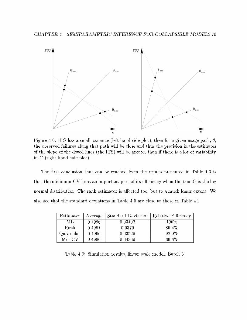
CHAPTER 4. SEMIPARAMETRIC INFERENCE FOR COLLAPSIBLE MODELS 79
���
���
��������
��������
��������
����
����
��������
���������������������������������������������������������������������������������������������������������������������������������������������������������������������������������������������������������������������������������������������������������������������������������������������������������������������������������������������������������
���������������������������������������������������������������������������������������������������������������������������������������������������������������������������������������������������������������������������������������������������������������������������������������������������������������������������������������������������������
������������������������������������������������������������������������������������������������������������������������������������������������������������������������������������������������������������������������������������������������������������������������������������������������������������
������������������������������������������������������������������������������������������������������������������������������������������������������������������������������������������������������������������������������������������������������������������������������������������������������������
���������������������������������������������������������������������������������������������������������������������������������������������������������������������������������������������������������������������������������������������������������������������������������������������������������������������������������������������������������������������������������������������������������������������������������������������������������������������������������������������������������������������������������������������������������������������������������������������������������������������������������������������������������������������������������������������������������������������������������������������������������������������������������������������������������������������������������������������������������������������������������������������������������������������������������������������������������������������������������������������������������������������������������������������������������������������������
���������������������������������������������������������������������������������������������������������������������������������������������������������������������������������������������������������������������������������������������������������������������������������������������������������������������������������������������������������������������������������������������������������������������������������������������������������������������������������������������������������������������������������������������������������������������������������������������������������������������������������������������������������������������������������������������������������������������������������������������������������������������������������������������������������������������������������������������������������������������������������������������������������������������������������������������������������������������������������������������������������������������������������������������������������������������������
���������������������������������������������������������������������������������������������������������������������������������������������������������������������������������������������������������������������������������������������������������������������������������������������������������������������������������������������������������������������������������������������������������������������������������������������������������������������������������������������������������������������������������������������������������������������������������������������������������������������������������������������������������������������������������������������������������������������������������������������������������������������������������������������������������������������������������������������������������������������������������������������������������������������������������������������������������������������������������������������������������������������������������������������������������������������������
���������������������������������������������������������������������������������������������������������������������������������������������������������������������������������������������������������������������������������������������������������������������������������������������������������������������������������������������������������������������������������������������������������������������������������������������������������������������������������������������������������������������������������������������������������������������������������������������������������������������������������������������������������������������������������������������������������������������������������������������������������������������������������������������������������������������������������������������������������������������������������������������������������������������������������������������������������������������������������������������������������������������������������������������������������������������������
���������������������������������������������������������������������������������������������������������������������������������������������������������������������������������������������������������������������������������������������������������������������������������������������������������������������������
���������������������������������������������������������������������������������������������������������������������������������������������������������������������������������������������������������������������������������������������������������������������������������������������������������������������������
������������������������������������������������������������������������������������������������������������������������������������������������������������������������������������������������������������������������������������������������������������������������������
������������������������������������������������������������������������������������������������������������������������������������������������������������������������������������������������������������������������������������������������������������������������������
������
������0.05
x
y(x) y(x)
x
θθ
θ
θ θ
θ
0.950.50
0.05
0.95 0.50
Figure 4.6: If G has a small variance (left hand side plot), then for a given usage path, �,the observed failures along that path will be close and thus the precision in the estimatesof the slope of the doted lines (the ITS) will be greater than if there is a lot of variability
in G (right hand side plot).
The �rst conclusion that can be reached from the results presented in Table 4.9 is
that the minimum CV loses an important part of its e�ciency when the true G is the log
normal distribution. The rank estimator is a�ected too, but to a much lesser extent. We
also see that the standard deviations in Table 4.9 are close to those in Table 4.2.
Estimator Average Standard Deviation Relative E�ciency
ML 0.4996 0.03402 100%Rank 0.4997 0.0379 80.4%
Quasi-like. 0.4996 0.03529 92.9%
Min CV 0.4996 0.04369 60.6%
Table 4.9: Simulation results, linear scale model, Batch 5.

CHAPTER 4. SEMIPARAMETRIC INFERENCE FOR COLLAPSIBLE MODELS 80
Batch 6
We simulated Batch 6 from the linear scale model t�(x) = (1 � 0:5)x+ 0:5�x with
1. G �log normal(6:7; 0:832);
2. atan(�) � Uniform(0; �=2).
From Table 4.10, it is clear that the minimum CV estimator is badly a�ected by the
choice of a log normal distribution with high coe�cient of variation, even if there is large
variability observed usage paths.
Estimator Average Standard Deviation Relative E�ciency
ML 0.4990 0.08137 100%Rank 0.4993 0.08818 85.2%
Quasi-like. 0.4991 0.09323 76.2%Min CV 0.4994 0.1696 23.0%
Table 4.10: Simulation results, linear scale model, Batch 6.
Batch 7
We simulated Batch 7 from the linear scale model t�(x) = (1 � 0:5)x+ 0:5�x with
1. G �log normal(6:7; 0:352);
2. ln � � N(2:37; 0:572).
Once again, we observe the same probability mass at �̂ = 1 for the rank estimator and
the same extreme volatility with the other estimators in Table 4.11 as we had in Table
4.6.

CHAPTER 4. SEMIPARAMETRIC INFERENCE FOR COLLAPSIBLE MODELS 81
Estimator Average Standard Deviation Mean Squared Error
ML 0.5449 0.1957 0.04029Rank 0.8116 0.2081 0.1404
Quasi-like. 0.5418 0.1972 0.04064
Min CV 0.5423 0.2241 0.05199
Table 4.11: Simulation results, linear scale model, Batch 7.
Batch 8
We simulated Batch 8 from the linear scale model t�(x) = (1 � 0:5)x+ 0:5�x with
1. G �log normal(6:7; 0:852);
2. ln � � N(2:37; 0:572).
Estimator Average Standard Deviation Mean Squared Error
ML 0.5784 0.3141 0.1048Rank 0.9009 0.1749 0.1913
Quasi-like. 0.5610 0.3209 0.1067
Min CV 0.5209 0.3760 0.1418
Table 4.12: Simulation results, linear scale model, Batch 8.
If we compare the results from Batches 1 to 4 to the results from Batches 5 to 8, we
can see that the averages and standard errors of the estimators are roughly the same for
the ML and quasi-likelihood estimator. The fact that the standard deviations did not
change much for the quasi-likelihood is not surprising; the asymptotic variance formulas
of Section 4.2.1 only involve the �rst two moments of G and the observed variability of
the usage paths. The rank based and minimum CV estimators seem to have lost some
of their e�ciency, though. In the case of the former, this was not surprising as it was

CHAPTER 4. SEMIPARAMETRIC INFERENCE FOR COLLAPSIBLE MODELS 82
derived by substituting 0 for the derivative of the hazard function in the likelihood score.
Nevertheless, the e�ciency still remained good. The minimum CV estimator was badly
a�ected by the change of form in G, and it could not keep the great e�ciency shown
under the Weibull parameterization for G.
4.4.2 Multiplicative scale model
We repeated the same analysis, but this time with the multiplicative scale model. We
generated data from
Pr [X > xj�] = G[x��]; (4.39)
where we used a value of � = 0:5 and a few di�erent distributions for G and the distri-
bution of the usage paths, �. We simulated 2000 samples of size 102 in each batch. The
results were along the same line as with the linear scale model, except that the impact
of the distribution of the usage paths was not as dramatic as in the linear scale model.
Batch 1
We simulated Batch 1 from the multiplicative scale model with
1. G(u) = exp
���
u
1000
�3�;
2. atan(�) � Uniform(0; �=2).
Table 4.14 summarizes the simulation results for Batch 1. We can see that with G
being Weibull with small coe�cient of variation, the minimum CV is extremely e�cient.
The rank method also showed great e�ciency.

CHAPTER 4. SEMIPARAMETRIC INFERENCE FOR COLLAPSIBLE MODELS 83
� = 0:25 � = 0:50 � = 0:75
�0:05 �0:50 �0:95 �0:05 �0:50 �0:95 �0:05 �0:50 �0:95(0.0787) (1.0) (12.71) (0.0787) (1.0) (12.71) (0.0787) (1.0) (12.71)
x0:05 701.5 371.6 196.8 1324.4 371.6 104.2 2501 371.6 55.21
x0:50 1671 885.0 468.7 3155 885.0 248.3 5956 885.0 131.5
x0:95 2722 1442 763.5 5139 1442 404.4 9702 1442 214.2
Table 4.13: Percentiles of real time at failure given usage path, multiplicative scale model,
Batch 1.
Estimator Average Standard Deviation Relative E�ciency
ML 0.5005 0.02198 100.0%Rank 0.5005 0.02210 98.9%
Quasi-like. 0.5004 0.02418 82.6%Min CV 0.5005 0.02202 99.7%
OLS 0.5003 0.02849 59.5%
Table 4.14: Simulation results, multiplicative scale model, Batch 1.
Batch 2
We simulated Batch 2 from the multiplicative scale model with
1. G(u) = expn� u
1000
o;
2. atan(�) � Uniform(0; �=2),
following the same pattern as with the linear scale model. Again, we expect the standard
deviations to be about 2.75 times the ones from Table 4.14.
The minimum CV was seriously a�ected by the increase in the coe�cient of variation
of G in this batch. Except for the minimum CV estimator, the standard deviations from
Table 4.16 are close to 2.75 times the ones in Table 4.14, which is what we expected.
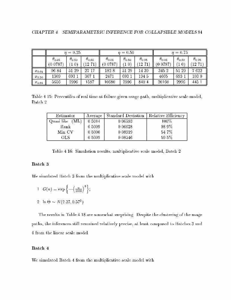
CHAPTER 4. SEMIPARAMETRIC INFERENCE FOR COLLAPSIBLE MODELS 84
� = 0:25 � = 0:50 � = 0:75
�0:05 �0:50 �0:95 �0:05 �0:50 �0:95 �0:05 �0:50 �0:95(0.0787) (1.0) (12.71) (0.0787) (1.0) (12.71) (0.0787) (1.0) (12.71)
x0:05 96.84 51.29 27.17 182.8 51.29 14.39 345.2 51.29 7.622
x0:50 1309 693.1 367.1 2471 693.1 194.5 4665 693.1 103.0
x0:95 5656 2996 1587 10680 2996 840.4 20160 2996 445.1
Table 4.15: Percentiles of real time at failure given usage path, multiplicative scale model,
Batch 2.
Estimator Average Standard Deviation Relative E�ciency
Quasi-like. (ML) 0.5014 0.06593 100%Rank 0.5009 0.06628 98.9%
Min CV 0.5000 0.08919 54.7%OLS 0.5009 0.08546 59.5%
Table 4.16: Simulation results, multiplicative scale model, Batch 2.
Batch 3
We simulated Batch 3 from the multiplicative scale model with
1. G(u) = exp
���
u
1000
�3�;
2. ln � � N(2:37; 0:572).
The results in Table 4.18 are somewhat surprising. Despite the clustering of the usage
paths, the inferences still remained relatively precise, at least compared to Batches 3 and
4 from the linear scale model.
Batch 4
We simulated Batch 4 from the multiplicative scale model with

CHAPTER 4. SEMIPARAMETRIC INFERENCE FOR COLLAPSIBLE MODELS 85
� = 0:25 � = 0:50 � = 0:75
�0:05 �0:50 �0:95 �0:05 �0:50 �0:95 �0:05 �0:50 �0:95(4.121) (10.70) (27.77) (4.121) (10.70) (27.77) (4.121) (10.70) (27.77)
x0:05 260.8 205.4 161.9 183.0 113.6 70.50 128.5 62.81 30.71
x0:50 621.2 489.4 385.5 436.0 270.6 167.9 306.0 149.6 73.15
x0:95 1012 797.1 628.0 710.2 440.8 273.5 498.4 243.7 119.2
Table 4.17: Percentiles of real time at failure given usage path, multiplicative scale model,
Batch 3.
Estimator Average Standard Deviation Relative E�ciency
ML 0.4987 0.06069 100%Rank 0.4987 0.06136 97.8%
Quasi-like. 0.4988 0.06519 86.6%OLS 0.4985 0.07591 63.9%
Min CV 0.4988 0.06131 98.0%
Table 4.18: Simulation results, multiplicative scale model, Batch 3.
1. G(u) = expn� u
1000
o;
2. ln � � N(2:37; 0:572).
Batch 5
We simulated Batch 5 from the multiplicative scale model with
1. G �log normal(6:7; 0:352);
2. atan(�) � Uniform(0; �=2).

CHAPTER 4. SEMIPARAMETRIC INFERENCE FOR COLLAPSIBLE MODELS 86
� = 0:25 � = 0:50 � = 0:75
�0:05 �0:50 �0:95 �0:05 �0:50 �0:95 �0:05 �0:50 �0:95(4.121) (10.70) (27.77) (4.121) (10.70) (27.77) (4.121) (10.70) (27.77)
x0:05 36.00 28.36 22.27 25.27 15.68 9.733 17.74 8.672 4.240
x0:50 486.5 383.3 301.9 341.5 211.9 131.5 239.7 117.2 57.30
x0:95 2103 1656 1305 1476 915.9 568.5 1036 506.5 247.6
Table 4.19: Percentiles of real time at failure given usage path, multiplicative scale model,
Batch 4.
Estimator Average Standard Error Relative E�ciency
Quasi-like. (ML) 0.4990 0.1804 100%Rank 0.4961 0.1825 97.7%OLS 0.4954 0.2277 62.8%
Min CV 0.5213 0.2342 59.4%
Table 4.20: Simulation results, multiplicative scale model, Batch 4.
Batch 6
We simulated Batch 6 from the multiplicative scale model with
1. G �log normal(6:7; 0:852);
2. atan(�) � Uniform(0; �=2).
Estimator Average Standard Error Relative E�ciency
OLS (ML) 0.4996 0.02301 100%
Rank 0.4996 0.02566 80.4%
Quasi-like. 0.4996 0.02386 93.0%Min CV 0.4996 0.02932 61.5%
Table 4.21: Simulation results, multiplicative scale model, Batch 5.

CHAPTER 4. SEMIPARAMETRIC INFERENCE FOR COLLAPSIBLE MODELS 87
Estimator Average Standard Error Relative E�ciency
OLS (ML) 0.4991 0.05456 100%Rank 0.4990 0.06084 80.4%
Quasi-like. 0.4991 0.06428 72.1%
Min CV 0.4998 0.1291 17.9%
Table 4.22: Simulation results, multiplicative scale model, Batch 6.
Batch 7
We simulated Batch 7 from the multiplicative scale model with
1. G �log normal(6:7; 0:352);
2. ln � � N(2:37; 0:572).
Estimator Average Standard Error Relative E�ciency
OLS (ML) 0.5012 0.06344 100%
Rank 0.5007 0.07024 81.6%Quasi-like. 0.5013 0.06531 94.3%Min CV 0.5012 0.08018 62.6%
Table 4.23: Simulation results, multiplicative scale model, Batch 7.
Batch 8
We simulated Batch 8 from the multiplicative scale model with
1. G �log normal(6:7; 0:852);
2. ln � � N(2:37; 0:572).
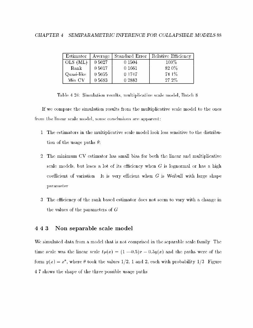
CHAPTER 4. SEMIPARAMETRIC INFERENCE FOR COLLAPSIBLE MODELS 88
Estimator Average Standard Error Relative E�ciency
OLS (ML) 0.5027 0.1504 100%Rank 0.5017 0.1661 82.0%
Quasi-like. 0.5055 0.1747 74.1%
Min CV 0.5683 0.2883 27.2%
Table 4.24: Simulation results, multiplicative scale model, Batch 8.
If we compare the simulation results from the multiplicative scale model to the ones
from the linear scale model, some conclusions are apparent:
1. The estimators in the multiplicative scale model look less sensitive to the distribu-
tion of the usage paths �;
2. The minimum CV estimator has small bias for both the linear and multiplicative
scale models, but loses a lot of its e�ciency when G is lognormal or has a high
coe�cient of variation. It is very e�cient when G is Weibull with large shape
parameter.
3. The e�ciency of the rank based estimator does not seem to vary with a change in
the values of the parameters of G.
4.4.3 Non separable scale model
We simulated data from a model that is not comprised in the separable scale family. The
time scale was the linear scale tP(x) = (1 � 0:5)x + 0:5y(x) and the paths were of the
form y(x) = x�, where � took the values 1/2, 1 and 2, each with probability 1/3. Figure
4.7 shows the shape of the three possible usage paths.

CHAPTER 4. SEMIPARAMETRIC INFERENCE FOR COLLAPSIBLE MODELS 89
y(x) θ =2.0 θ =
5
1.0
θ = 0.5
xt t t t t1 2 3 4
Figure 4.7: Shape of the usage paths for the model used in Section 4.4.3. Lines parallelto the doted lines represent various ages in the ideal time scale.
In Section 4.1, Lemma 4.1.1 gave su�cient conditions for the consistency of the min-
imum CV estimator. We cannot use the conclusion of Lemma 4.1.1 in this case because
the model is not of the separable scale form. Therefore, we do not know if the squared
CV of T (�) is uniquely minimized at � = 0:5, and hence if the minimum CV estimator
is consistent. However, if we compute CV 2[T (�)] numerically for some �xed distribution
G for this model, we can see that the value of � that minimizes it is � = 0:5. Figure 4.8
shows a plot of CV 2[T (�)] for this non separable scale model with G �Weibull(3, 1000).
From Figure 4.8, we expect the minimum CV estimator to be consistent. Also, we have
that the regularity conditions for the consistency of the ML and rank based estimators
are respected in this case, so we expect these two estimators to be consistent as well.

CHAPTER 4. SEMIPARAMETRIC INFERENCE FOR COLLAPSIBLE MODELS 90
eta
CV
[T(e
ta)]
0.0 0.2 0.4 0.6 0.8 1.0
0.2
0.4
0.6
0.8
Figure 4.8: CV 2[T (�)] as a function of � for the non separable scale model with G as inBatch 1. As we can see, the function seems to be uniquely minimized at � = 0:5. Wethus expect the minimum CV estimator to be consistent.
Batch 1
We �rst simulated Batch 1 using G(u) = expf�(u=1000)3g.
Estimator Average Standard Error Relative E�ciency
ML 0.4994 0.02131 100%Rank 0.4994 0.02175 96.0%
Min CV 0.4995 0.02147 98.5%
Table 4.25: Simulation results, nonseparable scale model, Batch 1.
Batch 2
We then simulated Batch 2 using G(u) = exp f�u=1000g.

CHAPTER 4. SEMIPARAMETRIC INFERENCE FOR COLLAPSIBLE MODELS 91
Estimator Average Standard Error Relative E�ciency
ML 0.4983 0.06236 100%Rank 0.4980 0.06361 96.1%
Min CV 0.4982 0.07903 62.3%
Table 4.26: Simulation results, nonseparable scale model, Batch 2.
Batch 3
We used the lognormal distribution to generate the failure times in Batches 3 and 4. In
Batch 3, the value of the location parameter was 6.7 and the value of the scale parameter
was 0.35.
Estimator Average Standard Error Relative E�ciency
ML 0.5045 0.02194 100%
Rank 0.5020 0.02471 78.9%Min CV 0.5022 0.02852 59.2%
Table 4.27: Simulation results, nonseparable scale model, Batch 3.
Batch 4
The value of the parameters of the lognormal distribution used to generate the failure
times in Batch 4 were 6.7 for the location parameter and 0.85 for the scale parameter.
Estimator Average Standard Error Relative E�ciency
ML 0.5071 0.05306 100%
Rank 0.5046 0.05783 84.2%
Min CV 0.5062 0.1094 23.5%
Table 4.28: Simulation results, nonseparable scale model, Batch 4.

CHAPTER 4. SEMIPARAMETRIC INFERENCE FOR COLLAPSIBLE MODELS 92
As expected, all three estimators had small bias, with the minimum CV and rank
estimators losing some e�ciency when G was the log normal survivor function.
4.4.4 Variance estimates and con�dence intervals
Another goal of this simulation study was to check the accuracy of the variance estimates
and the coverage of the con�dence intervals proposed in this chapter. Through simu-
lations, we looked at the coverage proportions of approximate 95% con�dence intervals
derived from the quasi-likelihood, minimum CV and rank based methods for the sepa-
rable scale models of Sections 4.4.1 and 4.4.2, and the rank-based method for the non
separable scale model of Section 4.4.3.
Table 4.29 gives the coverage proportions of approximate 95% con�dence intervals
given by �̂QL� 1:96
qdVar[�̂QL], where �̂
QLis the quasi-likelihood estimator and dVar[�̂
QL]
is the sample estimate of the variance given by (4.24). We used the same samples as the
ones used to study the the validity and e�ciency of the estimators, i.e. the same 2000
samples of size 102 used in the batches of Sections 4.4.1 and 4.4.2.
In addition to the data in Table 4.29, we observed that the intervals were not biased,
i.e. they missed the true value to the left just as often as they missed it to the right,
except for the \problem" Batches 3, 4, 7 and 8 for the linear scale model, where the
true parameter value was larger than the upper bound of the interval whenever the
interval did not include the true value. This tells us that the variance estimate tends
to underestimate the true variance in most batches, and that the distribution of the
estimator in the \problem" batches is not symmetric, as was shown in Figure 4.4 for the
rank-based estimator.
To derive approximate con�dence intervals using the minimum CV method, we used

CHAPTER 4. SEMIPARAMETRIC INFERENCE FOR COLLAPSIBLE MODELS 93
Linear scale model Multiplicative scale model
Batch 1 93.75% 94.35%Batch 2 92.70% 93.85%
Batch 3 91.70% 94.75%
Batch 4 84.35% 93.45%Batch 5 93.10% 93.40%Batch 6 91.65% 92.95%
Batch 7 91.40% 93.80%
Batch 8 84.35% 93.45%
Table 4.29: Coverage proportions of approximate 95% con�dence intervals, quasi-likelihood estimator, Batches 1-8 of Sections 4.4.1 (linear scale model) and 4.4.2. (multi-
plicative scale model).
the percentile bootstrap method described by Efron and Tibshirani (1993). This method
being rather computationally intensive (for each sample, we had to generate 1000 boot-
strap samples), we limited ourselves to the �rst 1000 samples of each batch, rather than
the full 2000 samples, and we only carried out the simulations for the eight batches of
Section 4.4.1, the minimum CV estimator having a closed form solution under linear time
scale models. The results are summarized in Table 4.30.
Linear scale model
Batch 1 94.0%
Batch 2 91.1%
Batch 3 94.4%
Batch 4 92.6%Batch 5 92.3%
Batch 6 91.8%Batch 7 92.9%
Batch 8 90.6%
Table 4.30: Coverage proportions of approximate 95% con�dence intervals, minimum CV
estimator, Batches 1-8 of Sections 4.4.1 (linear scale model).

CHAPTER 4. SEMIPARAMETRIC INFERENCE FOR COLLAPSIBLE MODELS 94
The results in Table 4.30 show that the coverage of the percentile bootstrap inter-
vals is lower than 95%. However, these percentile intervals are rather crude and can
easily be improved upon if one is willing to pay the computational price. Efron and
Tibshirani (1993, Chapter 14) describe the BCamethod, which is an improvement of the
percentile bootstrap method. It is extremely computationally intensive, and therefore its
coverage is rather di�cult to assess through a simulation study.
We also looked at coverage proportions of 95% con�dence intervals obtained using the
rank-based score. These intervals were derived using two versions of formula 4.31: one
in which the interval was f� : U2(�)=V (�) � �21;0:95g and one in which the interval was
f� : U2(�)=V (�̂) � �21;0:95g. The results are summarized in Table 4.31.
Linear scale model Multiplicative scale model
using V (�) using V (�̂) using V (�) using V (�̂)
Batch 1 94.25% 94.75% 94.65% 94.90%Batch 2 94.25% 96.55% 94.65% 94.90%
Batch 3 94.35% 55.25% 94.95% 95.20%Batch 4 94.35% 47.70% 94.95% 95.20%Batch 5 94.15% 95.20% 93.75% 94.55%Batch 6 94.15% 96.50% 93.75% 94.55%
Batch 7 94.65% 55.40% 94.50% 95.00%
Batch 8 94.65% 47.70% 94.50% 95.00%
Table 4.31: Coverage proportion of 95% con�dence intervals, rank-based estimator,
Batches 1-8 of Sections 4.4.1 and 4.4.2.
Both types of rank-based con�dence intervals seem to perform relatively well. From
this small simulation study, we have no evidence that the intervals based on V (�̂) are more
appropriate than the intervals based on V (�) in any case, except in the \problem cases"
3, 4, 7 and 8, where the coverage of the intervals based on V (�) looks more stable and
accurate. The bad coverage of the intervals based on V (�̂) for those \problem batches"

CHAPTER 4. SEMIPARAMETRIC INFERENCE FOR COLLAPSIBLE MODELS 95
is due to the fact that in a high proportion of the simulated samples (see histogram in
Figure 4.4), the estimated value of � was 1.0, which is far from the true value of 0.5,
hence the bad coverage of the intervals.
The rank-based intervals also have good coverage under the non separable scale model
of Section 4.4.3. We give simulation results for this model in the next section on censored
data simulations.
4.4.5 Censored data simulations
According to Lin and Ying (1995), the rank based method should also work for censored
samples, as long as the real times at failure and the censoring real times are independent,
given the usage paths. We simulated samples from a few of the models studied above,
but we introduced censoring.
More precisely, we generated censoring real times independently of the failure times.
We simulated the censoring times in the real time scale as censoring is more likely to
happen in real time in most applications. The censoring times were normally distributed,
with the mean and variance chosen so as to achieve speci�ed censoring proportions.
We simulated the same samples as the ones used in Batch 1 for both the linear and
multiplicative scale models (Sections 4.4.1 and 4.4.2), but we censored those samples
using normally distributed censoring real times. We did the same for the samples used
in Batch 1 of the non-separable scale model of Section 4.4.3. The simulation results are
summarized in Table 4.32.
It is also of interest to know if the coverage of the con�dence intervals based on
1These bad results are due to an important probability mass at �̂ = 1, i.e. the rank estimator identi�esy as the ITS in a large proportion of samples.

CHAPTER 4. SEMIPARAMETRIC INFERENCE FOR COLLAPSIBLE MODELS 96
Linear scale Mult. scale Non-separable scale
Censoring % �̂ std. dev. �̂ �̂ std. dev. �̂ �̂ std. dev. �̂
0% 0.5004 0.03193 0.5005 0.02210 0.4991 0.02178
20% 0.5027 0.04271 0.5022 0.03179 0.5003 0.02933
60% 0.5154 0.1015 0.5046 0.05422 0.58711 0.18671
Table 4.32: Simulations results, censored samples.
the rank score function is good for both censored and uncensored samples. Table 4.33
summarizes the results of big batches of 10,000 simulations of samples of size 102 from
the models used in Batch 1 of Sections 4.4.1 (linear scale model), 4.4.2 (multiplicative
scale model) and 4.4.3 (non separable scale model).
Linear scale Mult. scale Non-separable scale
censored using V (�) using V (�̂) using V (�) usingV (�̂) using V (�) using V (�̂)
0% 94.58% 95.19% 94.90% 94.92% 94.88% 95.58%
20% 94.78% 94.74% 94.85% 95.17% 95.01% 95.04%
60% 94.95% 92.74% 94.21% 94.97% 95.63% 89.87%
Table 4.33: Coverage of rank score based 95% con�dence intervals, censored samples.
From this small study, we see that the rank based method still gives good results
when we have censored data. The coverage of the 95% con�dence intervals was always
very close to 95%, except when we used V (�̂) in highly censored samples, in which
case the con�dence intervals derived using V (�) were still very accurate. If we consider
the coverage proportions for all the simulations done with the rank-based method, it is
probably safer to use the intervals computed using V (�) rather than V (�̂); the former
may give a coverage slightly lower than 95% in most situations, but their coverage was
never worse than 93.75%, compared to some coverages that were as low as 47.70% or

CHAPTER 4. SEMIPARAMETRIC INFERENCE FOR COLLAPSIBLE MODELS 97
55.25% for the latter.
4.4.6 Simulation summary
From these simulations, we can reach the following general conclusions:
1. The precision in the time scale parameter estimators increases with the variability
in the observed usage paths;
2. The precision in the time scale parameter estimators increases when the coe�cient
of variability of the distribution G decreases;
3. Under the linear scale model, the properties of every estimator are seriously a�ected
by changes in G or in the path distribution;
4. Under the multiplicative scale model, the precision of the estimators is still a�ected
by changes in G or in the path distribution, but to a lesser extent;
5. The rank based method seems to be the semiparametric method of choice. The
coverage of the con�dence intervals was always good and the relative e�ciency of
the estimators was always high under all choices of G. Moreover, it can readily
handle censoring, which is not the case with the other semiparametric methods
studied.
From these conclusions, the �rst recommendation that stands out is to get samples
with as much variability in the usage paths as possible. As we have seen, a sample size
as large as 100 was nowhere near enough for precise inference with the linear scale when
there was not much variability in the sample paths. However, when the variability in
the sample paths is large, samples of size as small as 30 can lead to precise inference, as

CHAPTER 4. SEMIPARAMETRIC INFERENCE FOR COLLAPSIBLE MODELS 98
will be seen in the data analyses of Chapter 6. If one wishes to design an experiment
in order to identify an ITS, one must make sure that units will be run under as many
di�erent usage patterns as possible; trying to derive an ITS from a sample of items used
under very similar conditions is useless. This implies that the use of collapsible models
for inference is more appropriate when the data are from populations with heterogeneous
usage histories, rather than populations where the units are all used in an homogeneous
way. We give examples of those two types of populations in Chapter 6.
As far as the choice of inference method is concerned, the rank based estimator seems
to be the most robust semiparametric estimator considered in this chapter, and this at
a very low cost in e�ciency. It did not lose much e�ciency under changes in the value
of the parameters of G, and when the form of G changed, it seemed to be the least
a�ected of the estimators. In the few cases in which this estimator broke down, the other
methods (including parametric ML) were also doing quite poorly, as precise inference was
not possible. In addition, the rank based estimator readily handled censored samples, in
which case it still had small bias. Moreover, the con�dence intervals derived from the
rank based estimator score function showed accurate coverage.

Chapter 5
Some other methods and
applications
In this chapter, we brie y address a couple of issues that have been left out of our
treatment of alternative time scales up to this point. More precisely, we consider non-
parametric estimation of the time scale function, tP(x), in Section 5.1 and we look at
potential applications of collapsible models in Section 5.2. Hopefully, further research
will lead to a more thorough development of these methods and applications.
5.1 Ideas for nonparametric inference
A discussion of nonparametric estimation methods for the time scale function tP(x) is
virtually absent from the literature. It would however be very useful as we do not know
before hand which form of ITS is more appropriate for a given problem. In this section, we
give some insight on how contours of the function tP(x) = �[yP(x)] could be traced from
a sample su�ciently large. The idea remains the same as for semiparametric estimation:
99

CHAPTER 5. SOME OTHER METHODS AND APPLICATIONS 100
exploit the fact that the distribution of the failure time in the ITS is the same along each
usage path.
5.1.1 Method based on grouped usage paths
If we are lucky enough to have many observations from only a few sample paths, what
we can do is link the corresponding quantiles of XjP from path to path and draw non-
parametric age curves this way. We can also use this idea if we have several usage paths;
all we need then is a method to group paths that are similar together and treat all the
usage paths within a group as a single path. Here is the algorithm that describes this
idea in more detail:
Algorithm 5.1
1. Split the data into K groups so that observations with similar usage paths are in
the same group.
2. For each group, identify a median or a mean path and then treat all the observations
within the group as if they came from that median/mean usage path.
3. Choose R quantiles �1; : : : ; �R and estimate these R quantiles of X on each of the
K median/mean paths.
4. For each of the R quantiles, link the corresponding quantile of X from all K me-
dian/mean paths using segments, planes or hyper-planes (depending on the dimen-
sion of the problem). These segments, planes or hyper-planes trace \quantile (age)
surfaces" that are similar to the elevation lines that we �nd on topographical maps.
5. These quantile (age) curves should have roughly the same form as the ITS.
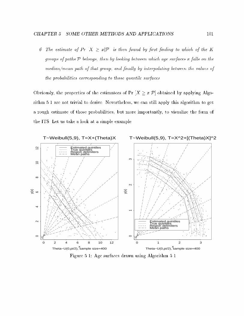
CHAPTER 5. SOME OTHER METHODS AND APPLICATIONS 101
6. The estimate of Pr [X � xjP] is then found by �rst �nding to which of the K
groups of paths P belongs, then by looking between which age surfaces x falls on the
median/mean path of that group, and �nally by interpolating between the values of
the probabilities corresponding to those quantile surfaces.
Obviously, the properties of the estimators of Pr [X � xjP] obtained by applying Algo-
rithm 5.1 are not trivial to derive. Nevertheless, we can still apply this algorithm to get
a rough estimate of those probabilities, but more importantly, to visualize the form of
the ITS. Let us take a look at a simple example.
..
.
.
.
.
.
.
.
.
.
.
.
.
.
.
.
.
.
.
.
.
.
.
.
.
.
.
.
.
.
. .
.
.
.
.
.
.
.
.
.
.
.
.
.
.
.
.
.
..
.
.
.
.
.
.
.
..
.
.
..
.
.
..
..
.
.
.
.
.
..
.
.
. .
. .
.
.
..
.
..
.
..
.
.
.
.
.
.
.
.
.
.
.
.
.
.
.
.
.
.
.
.
.
.
.
.
. .
.
.
.
.
.
.
..
..
.
.
.
.
.
.
.
..
.
.
.
.
.
.
..
. .
.
.
.
..
.
.
.
.
.
.
.
.
.
.
.
.
.
.
..
.
.
.
.
.
.
..
.
.
.
.
.
.
.
.
.
. .
.
.
.
..
.
.
.
.
.
..
..
.
.
.
.
.
.
.
.
.
.
.
.
.
.
..
. .
.
..
.
.
.
.
.
.
..
.
.
.
.
.
..
.
.
.
.
.
.
.
..
.. .
.
.
.
.
.
.
.
.
.
.
.
.
.
..
.
.
.
.
.
.
.
.
.
.
.
.
.
.
.
.
.
.
.
.
.
.
.
. .
.
.
..
.
.
.
.
.
..
.
..
..
.
.
.
. .
.
.
.
.
..
.
.
.
.
.
.
.
.
.
.
.
.
..
.
.
.
..
.
.
.
.
.
.
.
.
.
.
.
.
..
.
.
.
.
.
.
.
.
.
.
.
.
.
.
.
.
.
.
.
.
.
.
.
.
.
.
.
.
.
.
. .
.
.
.
.
.
.
.
..
.
.
.
.
.
.
.
.
x
y(x)
0 2 4 6 8 10 12
02
46
810
12 Estimated quintilesTrue quintilesRegion delimitersMean paths
T~Weibull(5,9), T=X+(Theta)X
Theta~U(0,pi/2), sample size=400
.
.
.
.
.
.
.
.
.
.
.
.
.
..
.
.
.
.
.
.
.
.
.
.
.
.
.
. .
.
.
.
.
.
.
.
.
.
..
.
. ..
.
.
.
.
.
..
.
.
.
.
. .
.
.
.
.
.
.
.
.
.
.
.
.
.
.
.
.
..
.
.
.
.
..
.
.
.
.
.
.
.
.
.
.
.
.
..
.
.
.
.
.
.
.
.
.
.
.
.
.
..
.
.
.
.
..
.
.
.
.
.
.
.
.
..
.
.
.
.
.
.
.
.
.
.
.
.
.
.
.
..
.
.
.
.
...
.
.
.
. .
.
. .
.
.
.
.
.
.
.
.
.
.
.
.
.
.
.
..
..
.
..
.
.
.
.
..
.
.
.
.
.
.
.
.
.
.
.
.
.
.
.
.
.
.
.
.
. .
.
.
.
.
.
.
.
.
.
.
.
.
.
.
..
.
.
.
.
.
.
..
. ..
.
.
.
.
.
.
.
.
.
.
.
.
..
.
.
..
.
..
.
.
.
.
.
.
.
.
.
.
.
.
.
.
.
.
.
.
.
.
.
.
.
.
.
.
.
.
.
.
.
.
.
.
.
.
.
.
.
.
.
.
.
.
.
.
.
. .
.
.
.
.
.
.
..
.
.
.
.
. .
.
.
.
.
.
.
.
.
.
.
.
.
.
..
.
.
.
..
.
.
.
..
.
.
.
.. .
.
.
.
.
.
.
.
.
.
. .
..
.
.
.
.
.
...
.
. .
.
. .
.
.
.
.
.
.
.
. .
.
.
.
.
.
.
.
.
..
.
.
.
x
y(x)
0 1 2 3
01
23
Estimated quintilesTrue quintilesRegion delimitersMean paths
T~Weibull(5,9), T=X^2+[(Theta)X]^2
Theta~U(0,pi/2), sample size=400
Figure 5.1: Age surfaces drawn using Algorithm 5.1.

CHAPTER 5. SOME OTHER METHODS AND APPLICATIONS 102
Example 5.1.1 Suppose we observe failure times coupled with one usage measure y(x) =
�x for each individual. We would like to know if a TS of the form �[x; y(x)] = x + �y
is ideal. Using Algorithm 5.1, we can split the positive quadrant into, say, 4 \slices" (see
Figure 5.1), treat all the data as if they were coming from the usage path at the center
of their respective slice, and link the quintiles from slice to slice with segments. The �rst
plot in Figure 5.1 shows this method applied to data simulated from G(x+ y), where T =
X + y(X) is generated from G, a Weibull distribution, and where � = arctan[y(X)=X]
comes from a uniform distribution on (0; �=2). The second plot shows the same method
applied to data coming from the same model except that now T = X2+y(X)2. As we can
see, the age curves on both plots roughly agree with the form of their corresponding ITS.
The method described in Algorithm 5.1 needs re�nement. Perhaps smoothing the age
curves using polynomials or other means could help the e�ciency. However, no matter
how good the method is, it will always require substantial variability between the usage
paths and a large number of observations in order to lead to sensible age curves.
5.1.2 Nonparametric quantile regression
Suppose that we have a pair of real random variables (X; Y ), with
Pr [Y � yjX = x] = Fx(y): (5.1)
Nonparametric quantile regression consists in estimating the quantiles of Fxfor all x
without making any parametric assumptions about Fx(�). This problem has been con-
sidered by various authors in di�erent frameworks. Good references on the topic include
Lejeune and Sarda (1988), Dabrowska (1987), Bhattacharya and Gangopadhyay (1990)

CHAPTER 5. SOME OTHER METHODS AND APPLICATIONS 103
and Cole and Green (1992).
In our collapsible model setup, we are interested in estimating the function �[x; y(x)]
in
Pr [X > xjP] = G(�[x; y(x)]):
If y(x) is a parametric path of the form y(x) = �x, then our problem simpli�es to
nonparametrically estimating the quantiles of Pr [X > xj�]. This is equivalent to the
nonparametric quantile regression problem.
Unfortunately, the methods described in the literature exhibit some serious edge e�ects
that deny us the possibility of identifying the form of the ITS. However, by the very
principles of the quantile regression methods, there is reason to believe that proper �ne
tuning of these methods should lead to good nonparametric estimates of the ITS function,
at least in the parametric usage path context.
Already, some methods have been proposed in the literature to remove edge e�ects
in nonparametric regression. For example, Hall and Wehrly (1991) propose a geometric
method for removing edge e�ects from kernel-based nonparametric regression estimators.
Such methods do not quite apply to our problem, but they are a step in the right direc-
tion. Perhaps an hybrid of one of those nonparametric quantile regression methods with
Algorithm 5.1 could lead to good estimates of the ITS function.
5.2 Applications of the collapsible model
Up to this point, the focus of this thesis has been on inference methods for collapsible
models. In this section, we want to outline a few potential uses and applications of these
models. We will assume that a collapsible model has been completely speci�ed and we

CHAPTER 5. SOME OTHER METHODS AND APPLICATIONS 104
will see how it can be used to solve practical problems such as the design of a maintenance
program or the evaluation of warranty costs.
Unlike what was the case with inference methods, prediction using a collapsible model
requires the speci�cation of a probability model for the usage path process. Many such
usage path models have been proposed in the literature, and we refer the reader inter-
ested in usage path modelling to Singpurwalla and Wilson (1993), Murthy, Iskandar and
Wilson (1995), Singpurwalla (1995) or Jewell and Kalb eisch (1996).
5.2.1 Maintenance programs
The great advantage of collapsible models is that they give a relatively simple way
of comparing units used under quite di�erent conditions (see Kordonsky and Gerts-
bakh (1993), Kordonsky and Gertsbakh (1994), Reinertsen (1996) or Gertsbakh and
Kordonsky (1997)). At any given clock time, one can compare two machines that have
been used di�erently simply by computing their age in the ITS. The advantage of col-
lapsible models in this case is that they allow for an easy calculation of the age in the
ITS.
Suppose we wish to schedule an inspection at the �rst quartile of the lifetime for
a population of devices used under di�erent conditions. Ideally, we would like a single
inspection program that would be valid under all possible usage scenarios. Assume that
the linear scale x+5y(x) is an ITS and that the 25th percentile of the lifetimes in this scale
is 100 units. Then for all the devices, the inspection should be held when x+5y(x) = 100.
Kordonsky and Gertsbakh (1994, 1997a) show how a linear combination of alternative
time scales can be used to derive maintenance programs.
Of course, it is possible to design such a maintenance program without a collapsible

CHAPTER 5. SOME OTHER METHODS AND APPLICATIONS 105
model. As long as a model for Pr [X � xjP] is available, all one has to do is monitor thevalue of Pr [X � xjP] for each device and then proceed with the inspection when this
probability reaches 0.25. However, device owners may have a harder time to calculate
this probability than the age of the device in a simple time scale. Moreover, calculation
of Pr [X � xjP] may require all the usage information P(x), whereas calculation of the
age in a collapsible models only requires the values of the usage measures at time x.
5.2.2 Prediction
Many applications of collapsible models involve the prediction of time to failure. When the
usage path P is entirely known, this problem is straightforward. Suppose that Pr [X >
xjP] = G[tP(x)] for some (not necessarily collapsible) ITS tP(x). Then
Pr [X > x+ sjX > s; P] =Pr [X > x+ sjP]Pr [X > xjP] ; 8x; s > 0
=G[tP(x+ s)]
G[tP(x)]:
When P is unknown, a probability model for the usage process, fY(x); x � 0g, isnecessary. Indeed,
Pr [X > x] = EP(x)fPr [X > xjP(x)g; 8x > 0 (5.2)
= EP(x)fG[tP(x)(x)]g;
where the expectation is taken over all possible usage histories up to time x.
If tP(x) is collapsible in y(x), i.e. tP(x) = �[y(x)], the problem is greatly simpli�ed
as the expectation in (5.2) is now taken over all the possible values of Y(x) rather than

CHAPTER 5. SOME OTHER METHODS AND APPLICATIONS 106
over all the possible usage histories up to time x:
Pr [X > x] = EP(x)fPr [X > xjP(x)g; 8x > 0
= EP(x)fG[tP(x)(x)]g
= EP(x)fG(�[Y(x)])g
= EY(x)fG(�[Y(x)])g:
In the case in which we observe a unit and its usage history up to time x and we wish
to know the probability that this unit will survive up to time x + s, the probability is
given by
Pr [X > x+ sjX > x;P(x)] = EY(x+s)fG(�[Y(x + s)])jP(x)gG(�[Y(x)])
; (5.3)
where the expectation is taken over all possible values ofY(x+s) given P(x) = fy(u); 0 �u � xg. If fY(u);u � 0g is a Markovian process then (5.3) further simpli�es to
Pr [X > x+ sjX > x;P(x)] = EY(x+s)fG(�[Y(x+ s)])jY(x) = y(x)gG(�[y(x)])
; (5.4)
where the expectation is now over all possible values of Y(x + s) given Y(x) = y(x).
5.2.3 An example of application: the warranty cost
A lot of attention has been devoted to methods for calculating warranty costs and war-
ranty reserves in the literature. Singpurwalla and Wilson (1993) survey the basic prin-
ciples underlying warranty cost calculations. In principle, calculating a warranty cost is
fairly straightforward; all that is needed is a warranty region and a probability model to

CHAPTER 5. SOME OTHER METHODS AND APPLICATIONS 107
compute the probability that a given item fails in that warranty region. In this section,
we see how a collapsible model can be used to derive such a probability model.
Suppose that we only observe one usage measure, say P = fy(x) : x � 0g, and that
the warranty region is a compact set in the positive quadrant of IR2, say W . Further,
assume that �[x; y(x)] is an ITS, i.e.
Pr [X � xjP] = G(�[x; y(x)])
for some distribution function G. Then the probability of failure in the warranty region
is given by
Pr [(X;Y (X)) 2 W ] =Z ZW
f(x; y) dxdy; (5.5)
where
f(x; y) =
"d
dxG(�[x; y])
#fY (x)(y);
fY (x)(y) being the pdf of the value of the usage measure at time x.
If the boundary ofW happens to be parallel to �[x; y(x)], i.e. W = fx; y : �[x; y] � kgfor some positive constant k, then probability (5.5) simply becomes
Pr [(X;Y (X)) 2 W ] = Pr [�[X;Y (X)] � k] = G(k): (5.6)
For example, if we have an ITS of the form �[x; y(x)] = x + 10y(x) with distribution
function G(u) = 1 � exp(�u ln �), and a warranty region of the form x + 10y(x) � k,
then the probability that an item fails while under warranty is given by 1� (1=�)k .
A collapsible model will therefore not necessarily lead to easier warranty cost calcu-
lation, unless the warranty region is parallel to the ITS. However, if a collapsible ITS is

CHAPTER 5. SOME OTHER METHODS AND APPLICATIONS 108
available, it could be used to design simple warranties that would lead to easy computa-
tion of warranty cost and reserve. Moreover, such warranties would be fair, in the sense
that no matter how the devices under warranty are used, the warranty extends to the
same proportion of the lifetime of the device for every user.
5.2.4 Accelerated testing
Another potential application of ITSs is in accelerated life testing. Nelson (1990, Chapter
10) and Meeker and Escobar (1998, Chapters 18-20) describe such procedures. Basically,
accelerated life tests (ALT) consist in testing devices under usage conditions much harsher
than \normal" usage in order to observe several failures during a relatively short test
period. The attraction of ITS's in such a setup is that results obtained under the ALT
can be extrapolated to normal usage conditions because of the independence of the failure
times in an ITS and the usage histories.
For example, suppose that for some device, t = x(1 + 5�) is an ITS, where x is real
time in weeks, say, and � is some usage rate. Then if we wish to design an ALT that
will be equivalent to the �rst 2/3 of the life of the devices under normal use, all that is
needed is the 66.7th percentile of the distribution of T , the lifetime in the ITS. Suppose
this percentile is t0:667 = 51 and that under normal conditions, a typical usage rate is
around � = 0:5. Then an ALT at accelerated usage rate of � = 10 would only have to
last one week, compared to 14.6 weeks under normal usage conditions. This ALT would
actually be equivalent to 2/3 of the lifetime distribution under any usage rate �, as long
as T is really an ITS.
Such tests are used in several �elds. For example in automobile system reliability,
test cars are driven under very harsh conditions, such as bumpy and twisty roads, highly

CHAPTER 5. SOME OTHER METHODS AND APPLICATIONS 109
variable temperatures, hard acceleration and braking, etc. for 40,000 miles, say, which
is supposed to be equivalent to, say, 150,000 miles under normal driving conditions. It
would be interesting to see if simple collapsible models based on the usage conditions
described in this example could be derived, and thus obtain equivalent mileages under
di�erent road/driving conditions.

Chapter 6
Data analysis and model assessment
In this chapter we analyze datasets available in the literature using some of the methods
introduced in Chapters 3 and 4. We also use these datasets to illustrate how various
hypotheses underlying collapsible models can be assessed.
Ideally, we would like to start every analysis by drawing nonparametric estimates of
the ITS, as in Example 5.1.1. Unfortunately, the few datasets available in the literature
are too small to allow for such nonparametric estimation. We can, nonetheless, �t models
with di�erent �xed forms for the ITS and assess their �t to the data. We then choose
the model that seems to be most appropriate.
6.1 Fatigue life of steel specimens
Kordonsky and Gertsbakh (1995a) considered the lifetime of steel specimens subjected
to periodic loading. The data are given in Appendix A.1. The 30 specimens were divided
into 6 groups of 5 units each, and the loading program (i.e. usage path) for each group was
a periodic sequence of high-level and low level stress cycles. Kordonsky and Gertsbakh
110
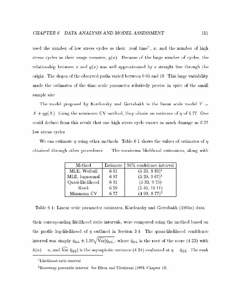
CHAPTER 6. DATA ANALYSIS AND MODEL ASSESSMENT 111
used the number of low stress cycles as their \real time", x, and the number of high
stress cycles as their usage measure, y(x). Because of the large number of cycles, the
relationship between x and y(x) was well approximated by a straight line through the
origin. The slopes of the observed paths varied between 0.05 and 18. This large variability
made the estimates of the time scale parameter relatively precise in spite of the small
sample size.
The model proposed by Kordonsky and Gertsbakh is the linear scale model T =
X + �y(X). Using the minimum CV method, they obtain an estimate of � of 6.77. One
could deduce from this result that one high stress cycle causes as much damage as 6.77
low stress cycles.
We can estimate � using other methods. Table 6.1 shows the values of estimates of �
obtained through other procedures. The maximum likelihood estimators, along with
Method Estimate 95% con�dence interval
MLE, Weibull 6.61 (5.33, 8.89)1
MLE, lognormal 6.97 (5.20, 9.67)1
Quasi-likelihood 6.91 (5.33, 9.75)
Rank 6.59 (5.40, 10.11)
Minimum CV 6.77 (4.99, 8.77)2
Table 6.1: Linear scale parameter estimates, Kordonsky and Gertsbakh (1995a) data.
their corresponding likelihood ratio intervals, were computed using the method based on
the pro�le log-likelihood of � outlined in Section 3.4. The quasi-likelihood con�dence
interval was simply �̂QL� 1:96
qdVar[�̂QL], where �̂
QLis the root of the score (4.23) with
h(u) = u, and dVar[�̂QL] is the asymptotic variance (4.24) evaluated at � = �̂
QL. The rank
1Likelihood ratio interval.
2Bootstrap percentile interval. See Efron and Tibshirani (1993, Chapter 13).
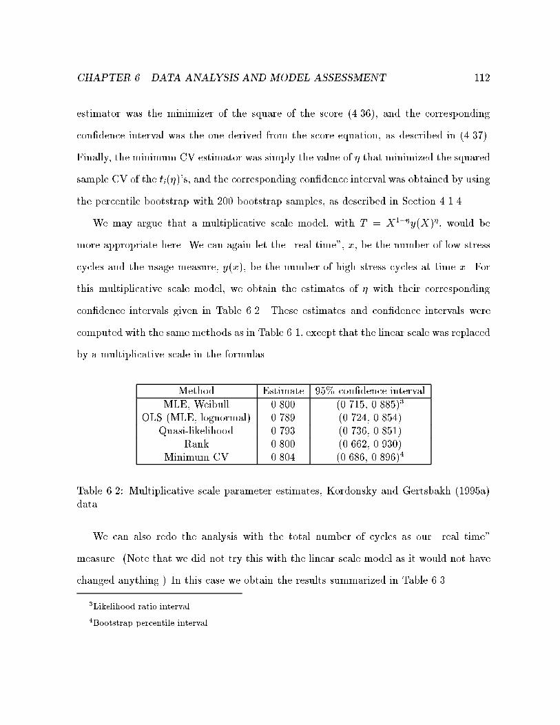
CHAPTER 6. DATA ANALYSIS AND MODEL ASSESSMENT 112
estimator was the minimizer of the square of the score (4.36), and the corresponding
con�dence interval was the one derived from the score equation, as described in (4.37).
Finally, the minimum CV estimator was simply the value of � that minimized the squared
sample CV of the ti(�)'s, and the corresponding con�dence interval was obtained by using
the percentile bootstrap with 200 bootstrap samples, as described in Section 4.1.4.
We may argue that a multiplicative scale model, with T = X1��y(X)�, would be
more appropriate here. We can again let the \real time", x, be the number of low stress
cycles and the usage measure, y(x), be the number of high stress cycles at time x. For
this multiplicative scale model, we obtain the estimates of � with their corresponding
con�dence intervals given in Table 6.2. These estimates and con�dence intervals were
computed with the same methods as in Table 6.1, except that the linear scale was replaced
by a multiplicative scale in the formulas.
Method Estimate 95% con�dence interval
MLE, Weibull 0.800 (0.715, 0.885)3
OLS (MLE, lognormal) 0.789 (0.724, 0.854)Quasi-likelihood 0.793 (0.736, 0.851)
Rank 0.800 (0.662, 0.930)Minimum CV 0.804 (0.686, 0.896)4
Table 6.2: Multiplicative scale parameter estimates, Kordonsky and Gertsbakh (1995a)data.
We can also redo the analysis with the total number of cycles as our \real time"
measure. (Note that we did not try this with the linear scale model as it would not have
changed anything.) In this case we obtain the results summarized in Table 6.3.
3Likelihood ratio interval.
4Bootstrap percentile interval.
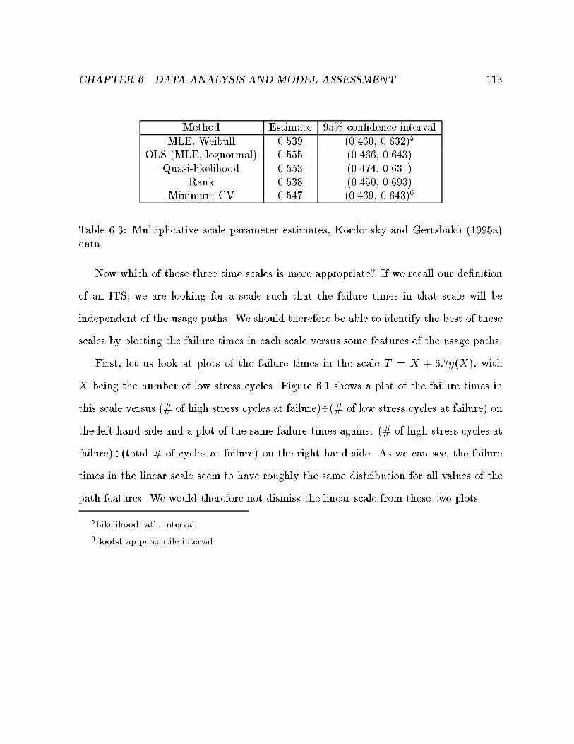
CHAPTER 6. DATA ANALYSIS AND MODEL ASSESSMENT 113
Method Estimate 95% con�dence interval
MLE, Weibull 0.539 (0.460, 0.632)5
OLS (MLE, lognormal) 0.555 (0.466, 0.643)
Quasi-likelihood 0.553 (0.474, 0.631)
Rank 0.538 (0.450, 0.693)Minimum CV 0.547 (0.469, 0.643)6
Table 6.3: Multiplicative scale parameter estimates, Kordonsky and Gertsbakh (1995a)
data.
Now which of these three time scales is more appropriate? If we recall our de�nition
of an ITS, we are looking for a scale such that the failure times in that scale will be
independent of the usage paths. We should therefore be able to identify the best of these
scales by plotting the failure times in each scale versus some features of the usage paths.
First, let us look at plots of the failure times in the scale T = X + 6:7y(X), with
X being the number of low stress cycles. Figure 6.1 shows a plot of the failure times in
this scale versus (# of high stress cycles at failure)�(# of low stress cycles at failure) on
the left hand side and a plot of the same failure times against (# of high stress cycles at
failure)�(total # of cycles at failure) on the right hand side. As we can see, the failure
times in the linear scale seem to have roughly the same distribution for all values of the
path features. We would therefore not dismiss the linear scale from these two plots.
5Likelihood ratio interval.
6Bootstrap percentile interval.

CHAPTER 6. DATA ANALYSIS AND MODEL ASSESSMENT 114
•
•
•
•
•
•
•
••
•
•
•
•
•
••
•
••
•
•
•
•
•
•
•
•
•
•
•
Scale T=X+6.7y(X)
(# high stress)/(# low stress)
failur
e tim
e in s
cale
T
0 5 10 15
3000
0040
0000
5000
0060
0000
•
•
•
•
•
•
•
••
•
•
•
•
•
••
•
••
•
•
•
•
•
•
•
•
•
•
•
Scale T=X+6.7y(X)
(# high stress)/(total # cycles)
failur
e tim
e in s
cale
T0.2 0.4 0.6 0.8
3000
0040
0000
5000
0060
0000
Figure 6.1: Failure times versus path features, scale T = X + 6:7y(X).
From the data given by Kordonsky and Gertsbakh (1995a) we can compute other
path features, like for instance the cumulative cycles�amplitude at failure, or the area
under the cycles�amplitude curve. If we plot the failure times in the scale T = X+6:7Y
versus these last two path features, as in Figure 6.2, we again cannot dismiss the linear
time scale, as there does not seem to be any trend in the plots.

CHAPTER 6. DATA ANALYSIS AND MODEL ASSESSMENT 115
•
•
•
•
•
•
•
••
•
•
•
•
•
••
•
••
•
•
•
•
•
•
•
•
•
•
•
cumulative cycles*amplitude
X+6.7
Y
10^7 2*10^7 4*10^7 6*10^7
3000
0040
0000
5000
0060
0000
•
•
•
•
•
•
•
••
•
•
•
•
•
••
•
••
•
•
•
•
•
•
•
•
•
•
•
area under cumulative cycles*amplitude
X+6.7
Y0 5*10^12 10^13 1.5*10^13
3000
0040
0000
5000
0060
0000
Figure 6.2: Failure times versus path features, scale T = X + 6:7y(X).
Let us now repeat the same procedure with the multiplicative scale T = X0:205y(X)0:795,
where X is, once again, the number of low stress cycles. The plot on the right hand side
of Figure 6.3 shows a de�nite trend; the failure times for average usage paths look larger
than the failure times for extreme usage paths. This means that the multiplicative scale
with the number of low stress cycles as measure of real time is not ideal.
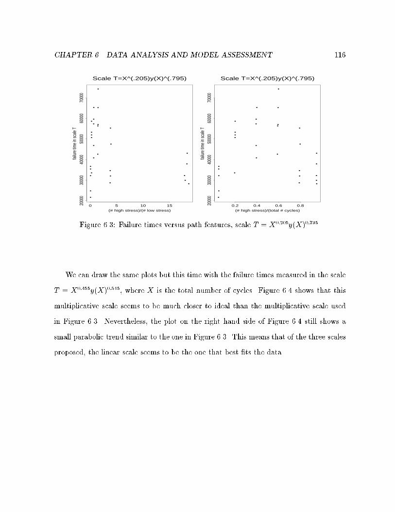
CHAPTER 6. DATA ANALYSIS AND MODEL ASSESSMENT 116
•
•
•
•
•
•
•
••
•
••
•
•
•
•
•
••
•
•
•
•
•
••
•
•
•
•
Scale T=X^(.205)y(X)^(.795)
(# high stress)/(# low stress)
failur
e tim
e in s
cale
T
0 5 10 152000
030
000
4000
050
000
6000
070
000
•
•
•
•
•
•
•
••
•
••
•
•
•
•
•
••
•
•
•
•
•
••
•
•
•
•
Scale T=X^(.205)y(X)^(.795)
(# high stress)/(total # cycles)
failur
e tim
e in s
cale
T0.2 0.4 0.6 0.820
000
3000
040
000
5000
060
000
7000
0
Figure 6.3: Failure times versus path features, scale T = X0:205y(X)0:795.
We can draw the same plots but this time with the failure times measured in the scale
T = X0:455y(X)0:545, where X is the total number of cycles. Figure 6.4 shows that this
multiplicative scale seems to be much closer to ideal than the multiplicative scale used
in Figure 6.3. Nevertheless, the plot on the right hand side of Figure 6.4 still shows a
small parabolic trend similar to the one in Figure 6.3. This means that of the three scales
proposed, the linear scale seems to be the one that best �ts the data.

CHAPTER 6. DATA ANALYSIS AND MODEL ASSESSMENT 117
•
•
•
•
••
•
••
•
•
•
•
•
•
•
•
••
•
•
•
•
•
•
•
•
•
•
•
Scale T=X^(.455)y(X)^(.545)
(# high stress)/(# low stress)
failur
e tim
e in s
cale
T
0 5 10 154000
050
000
6000
070
000
8000
090
000
1000
00
•
•
•
•
• •
•
••
•
•
•
•
•
•
•
•
••
•
•
•
•
•
•
•
•
•
•
•
Scale T=X^(.455)y(X)^(.545)
(# high stress)/(total # cycles)
failur
e tim
e in s
cale
T0.2 0.4 0.6 0.840
000
5000
060
000
7000
080
000
9000
010
0000
Figure 6.4: Failure times versus path features, scale T = X0:455y(X)0:545.
It is worth mentioning that in the case where y(x) = �x, a plot of xi��1iversus �
iwill
have the shape of a parabola facing downwards if the true ITS is of the form xi(1+ �2�i).
Similarly, a plot of xi(1+�2�i) versus �i will have the shape of a parabola facing upwards
when the true ITS is xi��1i. The fact that the plot on the right hand side of Figure 6.3 has
the shape of a parabola facing downwards is thus another argument favoring the choice
of a linear time scale.
As we mentioned at the beginning of Chapter 4, we can look at probability plots of
the failure times in the estimated ITS in order to �nd a suitable parametric form for G.
Let us look at Weibull and lognormal probability plots of the failure times in the scale
T = X + 6:7y(X). As we can see on Figure 6.5, there doesn't seem to be any evidence
against either distribution.

CHAPTER 6. DATA ANALYSIS AND MODEL ASSESSMENT 118
•
•
•
•
••
•••
••
••
•••
••••••
••••••
•
Weibull probability plotScale T=X+6.7y(X)
log(t)
log(-l
og(S
(t)))
12.6 12.8 13.0 13.2
-3-2
-10
1
•
•
•
•
•
•
•
••
•
•
•
•
•
•
•
•
••
•
•
•
•
•
•
•
•
•
•
•
Lognormal probability plotScale T=X+6.7y(X)
Quantiles of Standard Normal
log(t)
-2 -1 0 1 212
.612
.813
.013
.2
Figure 6.5: Weibull and lognormal probability plots, scale T = X + 6:7y(X).
Such probability plots cannot, however, be used to verify if a time scale is ideal. Figure
6.6 shows Weibull and lognormal probability plots for the times in the multiplicative scale
T = X0:205y(X)0:795, which, according to Figure 6.3, is not an ITS. As we can see, both
plots look \just as straight" as the plots from Figure 6.5, even though this multiplicative
scale is not ideal.

CHAPTER 6. DATA ANALYSIS AND MODEL ASSESSMENT 119
•
•
•
•
•••
•••
••
•••
••
•••
••••••
••
•
Weibull probability plotScale T=X^(.205)y(X)^(.795)
log(t)
log(-l
og(S
(t)))
10.2 10.4 10.6 10.8 11.0 11.2
-3-2
-10
1
•
•
•
•
•
•
•
••
•
••
•
•
•
•
•
••
•
•
•
•
•
•
•
•
•
•
•
Lognormal probability plotScale T=X^(.205)y(X)^(.795)
Quantiles of Standard Normal
log(t)
-2 -1 0 1 210
.010
.210
.410
.610
.811
.011
.2
Figure 6.6: Weibull and lognormal probability plots, scale T = X0:205y(X)0:795.
To conclude, we can perform a test to verify the �t of the overall model. Suppose we
choose the linear time scale T = X + �y(X) and the Weibull distribution for G, i.e.
Pr [X > xj�] = exp
8<:�"x(1 + ��)
�1
#�2
9=; :
We get �̂ = 6:61, �̂1 = 443; 190 and �̂2 = 5:61 as our time scale, distribution scale
and distribution shape parameter estimates, respectively. We can then divide the ideal
time scale in 5 intervals, say [0, 339,000), [339,000, 393,000), [393,000, 435,000), [435,000,
481,000) and [481,000, 1). We then compute the Pearson chi-squared statistic using
the times measured in the scale X + �̂y(X) as our observations. We obtain the results
summarized in Table 6.4.
The value of the test statistic is 0.574. Because we do not actually observe the

CHAPTER 6. DATA ANALYSIS AND MODEL ASSESSMENT 120
Interval Expected (Ei) Observed (O
i) (O
i�E
i)2=E
i
[0, 339,000) 5.98 7 0.174
[339; 000; 393; 000) 6.00 5 0.167[393; 000; 435; 000) 5.83 5 0.118
[435; 000; 481; 000) 6.03 6 0.000149
[481; 000; 1) 6.16 7 0.115
Total 30.0 30 0.574
Table 6.4: Chi-squared goodness-of-�t test, Kordonsky and Gertsbakh (1995a) data.
value of the times in the ITS, the usual chi-squared approximation cannot be used in
order to derive the signi�cance level of this test statistic. We can nonetheless estimate
this signi�cance level when needed using the model prescribed by the null hypothesis
(Pr [X > xjP] = G[x + �y(x)] with G Weibull) and the parametric bootstrap. In order
to simulate the usage paths, we can use resampling. Note that such computations were
not needed here, for the p-value is clearly high with a test statistic value as low as 0.574.
6.2 Fatigue life of aluminum specimen
Kordonsky and Gertsbakh (1997b) analyze data from another fatigue life experiment,
but this time on aluminum specimen. The experiment is described by Schijve and
Jakobs (1960) and the data are given in Appendix A.2. Kordonsky and Gertsbakh still
use a linear combination of two time scales, but this time they propose two di�erent ways
of measuring x and y. In the �rst approach, they de�ne x to be the cumulative number
of cycles at amplitudes 1.6, 2.0 or 2.75, and y to be the cumulative number of cycles at
amplitudes greater than 2.75 (see Appendix A.2, Table A.2). Using this approach and a
linear time scale model of the form T = X + �Y , we obtain an estimate of � of about

CHAPTER 6. DATA ANALYSIS AND MODEL ASSESSMENT 121
11.5 (Weibull and log normal MLEs and minimum CV). But if we plot the failure times
in this scale against the path number, we can see that the failure times seem to have
di�erent distributions for di�erent paths. This can be veri�ed by a Kruskal-Wallis test,
which leads to a p-value of 0.013. A multiplicative scale does not look more ideal than
this linear scale. If we use the model T = X1��Y �, we get that the estimate of � is 0.53,
and again the failure times in this scale look like they have di�erent distributions for
di�erent usage paths. The p-value of the Kruskal-Wallis test in this case is 0.009. Figure
6.7 shows plots of the failure times in the two scales mentioned above against the path
number.
•
••
•
•
•
•
•
•
•••
••
•
•
•••
••
•
••••
•
•
••
•
•
•
•
•
••
•
•
•
••
•
••
•
•
•
•
path number
X+11
.54Y
2 4 6 8 10 12 14
1000
1500
2000
2500
3000
3500
•
••
•
•
•
•
•
•
•••
••
•
•
•••
••
•
•••
•
••
••
•
•
•
•
•
•
•
•
•
•
••
•
••
•
•
•
•
path number
X^0.
47 Y
^0.5
3
2 4 6 8 10 12 14
200
300
400
Figure 6.7: Failure times in the estimated scale versus usage path index, Kordonsky and
Gertsbakh (1997b) data, �rst approach.
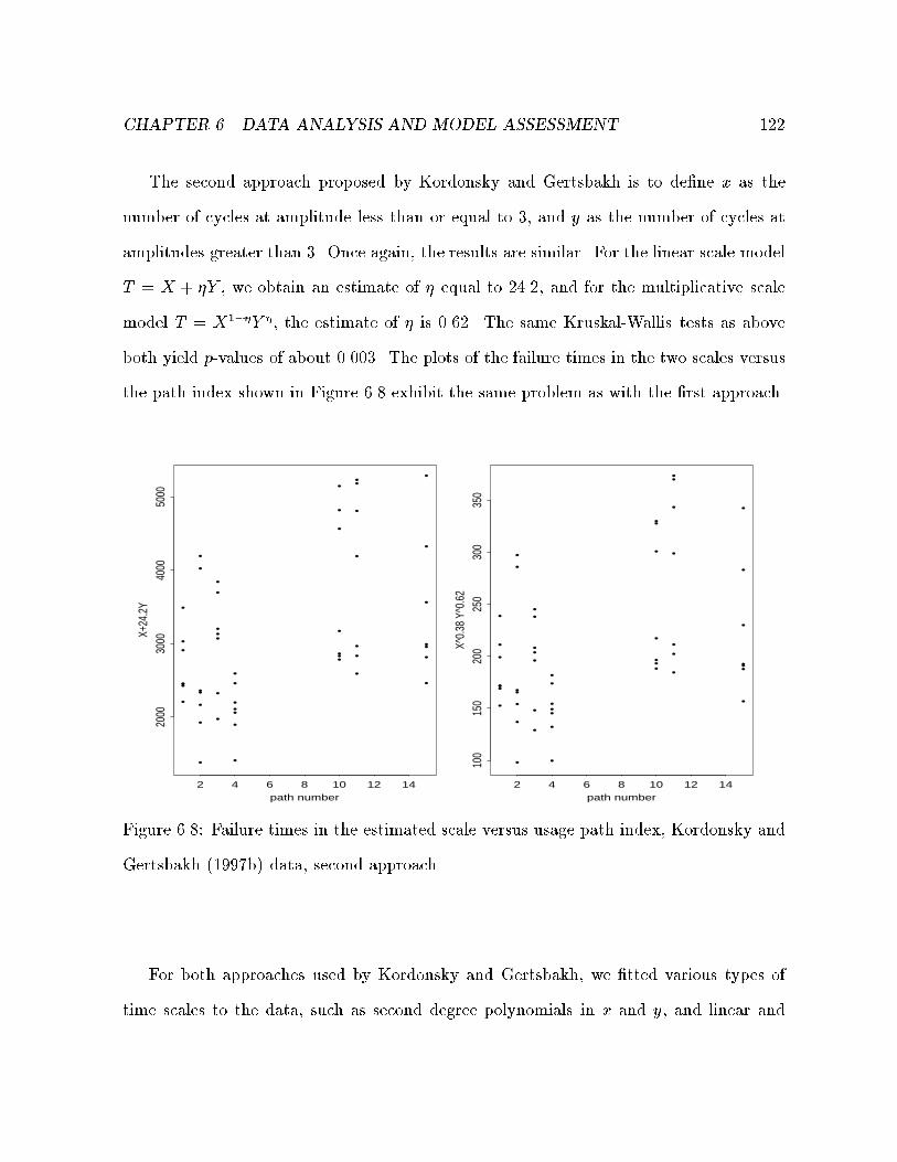
CHAPTER 6. DATA ANALYSIS AND MODEL ASSESSMENT 122
The second approach proposed by Kordonsky and Gertsbakh is to de�ne x as the
number of cycles at amplitude less than or equal to 3, and y as the number of cycles at
amplitudes greater than 3. Once again, the results are similar. For the linear scale model
T = X + �Y , we obtain an estimate of � equal to 24.2, and for the multiplicative scale
model T = X1��Y �, the estimate of � is 0.62. The same Kruskal-Wallis tests as above
both yield p-values of about 0.003. The plots of the failure times in the two scales versus
the path index shown in Figure 6.8 exhibit the same problem as with the �rst approach.
•
••
•
•
•
•
•
•
•••
••
•
•
•••
••
•
•••
•
••
••
•
•
•
•
•
•
•
•
•
•
••
•
••
•
•
•
•
path number
X+24
.2Y
2 4 6 8 10 12 14
2000
3000
4000
5000
•
••
•
•
•
•
•
•
•••
••
•
•
•••
••
•
•••
•
••
••
•
•
•
•
•
•
•
•
•
•
••
•
••
•
•
•
•
path number
X^0.
38 Y
^0.6
2
2 4 6 8 10 12 14
100
150
200
250
300
350
Figure 6.8: Failure times in the estimated scale versus usage path index, Kordonsky and
Gertsbakh (1997b) data, second approach.
For both approaches used by Kordonsky and Gertsbakh, we �tted various types of
time scales to the data, such as second degree polynomials in x and y, and linear and
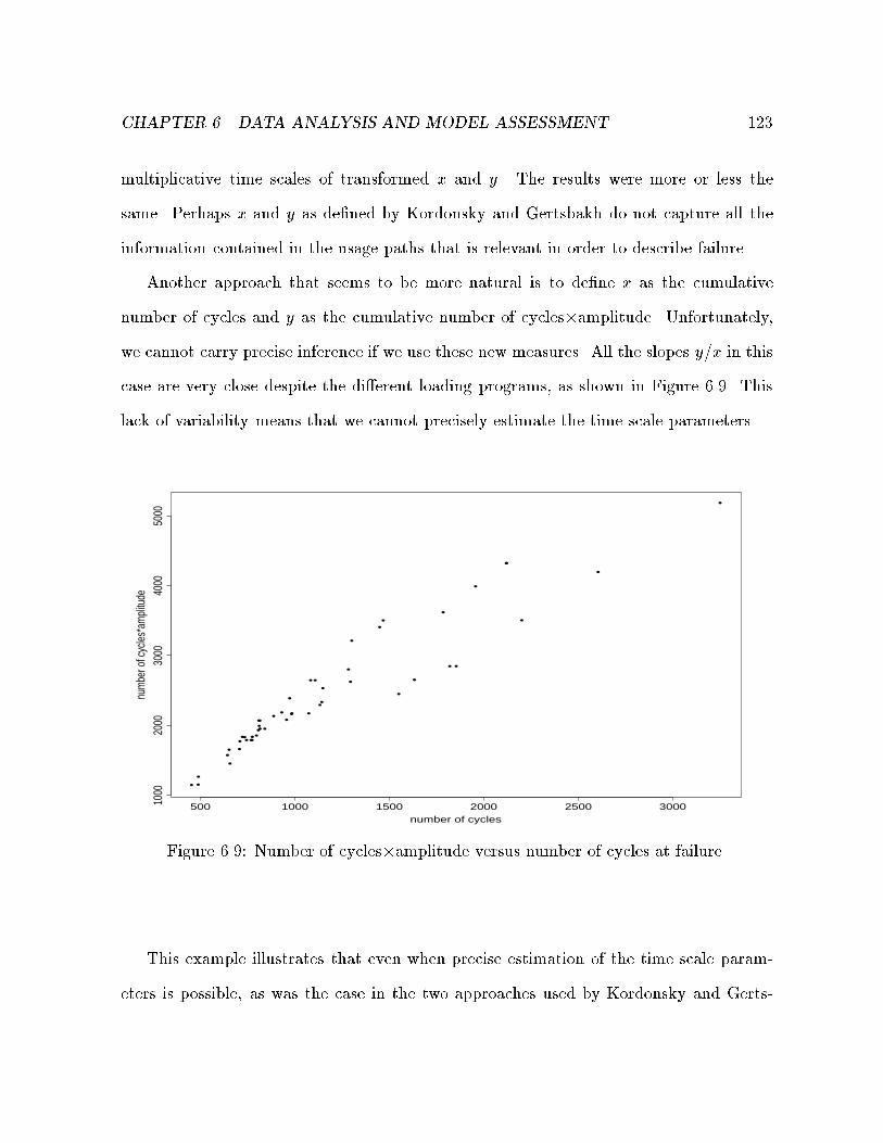
CHAPTER 6. DATA ANALYSIS AND MODEL ASSESSMENT 123
multiplicative time scales of transformed x and y. The results were more or less the
same. Perhaps x and y as de�ned by Kordonsky and Gertsbakh do not capture all the
information contained in the usage paths that is relevant in order to describe failure.
Another approach that seems to be more natural is to de�ne x as the cumulative
number of cycles and y as the cumulative number of cycles�amplitude. Unfortunately,we cannot carry precise inference if we use these new measures. All the slopes y=x in this
case are very close despite the di�erent loading programs, as shown in Figure 6.9. This
lack of variability means that we cannot precisely estimate the time scale parameters.
•
••
•
•
•
•
•
•
•••
••
••
•••
••
•
• •••
•
•
••
•
•
••
•
••
•
•
•
••
•
•
•
•
•
•
•
number of cycles
num
ber o
f cyc
les*a
mpli
tude
500 1000 1500 2000 2500 30001000
2000
3000
4000
5000
Figure 6.9: Number of cycles�amplitude versus number of cycles at failure.
This example illustrates that even when precise estimation of the time scale param-
eters is possible, as was the case in the two approaches used by Kordonsky and Gerts-

CHAPTER 6. DATA ANALYSIS AND MODEL ASSESSMENT 124
bakh (1997b), the estimated time scale obtained may not be ideal.
6.3 Cracks in the joint unit of the wing and fuselage
In aircraft reliability, engineers were interested in knowing what caused cracks in the joint
unit of the wing and fuselage. Two hypotheses were discussed:
1. the cracks were caused by the high frequency resonance produced by the engine
sound wave;
2. the cracks were due to the high stress sustained during landing.
The solution to the crack appearance problem under hypothesis 1. being completely
di�erent to that under hypothesis 2., it is obvious why the engineers were interested in
�nding which hypothesis was true.
Kordonsky and Gertsbakh (1993) consider this problem through a time scale approach.
The reasoning of Kordonsky and Gertsbakh is the following: if the cracks are caused by
high frequency resonance, then the total ight hours should be the ITS, whereas if cracks
are caused by the high stress of landing, then the cumulative number of landings should be
the ITS. The data given in Appendix A.3 are used by Kordonsky and Gertsbakh (1993).
Because they only observe interval censored data, Kordonsky and Gertsbakh cannot use
their usual semiparametric estimator of the time scale parameter. Their analysis thus
consists in �tting a parametric distribution to the data under both scales ( ight hours
and number of landings) separately via maximum likelihood, then choosing the scale that
yields the estimated distribution with the smaller coe�cient of variation. The number
of ight hours gives an estimated distribution with smaller coe�cient of variation than

CHAPTER 6. DATA ANALYSIS AND MODEL ASSESSMENT 125
cumulative number of landings for all three parametric families of distributions �tted to
the data. Kordonsky and Gertsbakh thus conclude that high frequency is the cause of
the cracks in the joint units.
Kordonsky and Gertsbakh (1993) did not consider scales that are a function of both
the number of ight hours and the number of landings. Let us assume a linear and
multiplicative form for the ITS, i.e. scales of the form (1 � �)(# of ight hours)+�(#
of landings) and (# of ight hours)1��(# of landings)�, respectively. If we �t a Weibull
and a lognormal distribution using both these scales, we obtain the pro�le log likelihoods
shown in Figures 6.10 and 6.11.
eta
lpro(
eta)
0.0 0.2 0.4 0.6 0.8 1.0
-23
-22
-21
-20
-19
Weibull profile log-likelihhod95% likelihood ratio interval
eta
lpro(
eta)
0.0 0.2 0.4 0.6 0.8 1.0
-23.
0-2
2.5
-22.
0-2
1.5
-21.
0-2
0.5
-20.
0
Lognormal profile log-likelihhod95% likelihood ratio interval
Figure 6.10: Pro�le log likelihood of the time scale parameter, linear scale model. The
plot on the left hand side is assuming a Weibull distribution, the plot on the right hand
side, a log normal.

CHAPTER 6. DATA ANALYSIS AND MODEL ASSESSMENT 126
eta
lpro(
eta)
0.0 0.2 0.4 0.6 0.8 1.0
-25
-24
-23
-22
-21
-20
Weibull profile log likelihood95% likelihood ratio interval
eta
lpro(
eta)
0.0 0.2 0.4 0.6 0.8 1.0
-24
-23
-22
-21
-20
Lognormal profile log likelihood95% likelihood ratio interval
Figure 6.11: Pro�le log likelihood of the time scale parameter, multiplicative scale model.
The plot on the left hand side is assuming a Weibull distribution, the plot on the right
hand side, a log normal.
In all cases, it looks like � = 0 (i.e., the ITS is the number of ight hours) is included
in the con�dence interval. Moreover, in the multiplicative scale case (the case in which
� is scale invariant), the likelihood over [0, 1] is maximized at � = 0 and the con�dence
interval is very narrow. This points to the same conclusion as that reached by Kordonsky
and Gertsbakh (1993).

CHAPTER 6. DATA ANALYSIS AND MODEL ASSESSMENT 127
6.4 Failure times and mileages for tractor motors
For predictive purposes, Singpurwalla and Wilson (1995) considered a joint model for
the time and cumulative mileage at failure for locomotive traction engines. The data are
given in Appendix A.4. We use this dataset to illustrate how data on time and cumulative
usage at failure do not necessarily allow for precise estimation of an ITS.
If we look at Table A.5, we notice that there is not much variability in the slopes
�. This is even more obvious when we look at the scatter plot of mileage versus time
at failure presented in Figure 6.12. Actually, if one �ts a simple linear regression model
through the origin to these data, one gets an R2 statistic of 97.6%. This means that
mileage and time at failure are almost constant multiples of each other and, therefore, it
will be nearly impossible to estimate the ITS parameters no matter what the model is.
For instance, if we look at the score function for the rank-based method with the
linear scale model t�= (1 � �)x + ��x sketched in Figure 6.13, we see that the score
increases slowly as � increases, rather than increasing or decreasing sharply to cross 0
somewhere between � = 0 and � = 1. Choosing a multiplicative scale model does not
solve the problem either, as shown on Figure 6.14. In this case the score slowly decreases
as � increases, without crossing 0 between 0 and 1.

CHAPTER 6. DATA ANALYSIS AND MODEL ASSESSMENT 128
•
•
••
• • • •
•
•
•
•• ••
• ••
•
••
• •
••
•
•
•
•
•
• •
•
•
•
•
•
•
•
•
Time (days)
Mile
age
(mile
s)
0 200 400 600 800 1000 1200
010
000
2000
030
000
4000
050
000
Figure 6.12: Mileage (miles) versus time (days) at failure for the locomotive tractionmotor data of Singpurwalla and Wilson (1995).
eta
U(eta
)
0.2 0.4 0.6 0.8 1.0
-8-6
-4-2
0
Figure 6.13: Rank score for the linear scale with the locomotive traction motor data.

CHAPTER 6. DATA ANALYSIS AND MODEL ASSESSMENT 129
eta
U(eta
)
0.0 0.2 0.4 0.6 0.8 1.0
-6-4
-20
Figure 6.14: Rank score for the multiplicative scale with the locomotive traction motor
data.
We get, as our estimate of �, �̂ = 1 with the linear scale model and �̂ = 0 with the
multiplicative scale model. In both cases, and for all the di�erent estimation methods,
the 95% con�dence intervals virtually covered the whole [0, 1] interval. This is not
surprising as knowing the value of time at failure is nearly equivalent to knowing the
value of cumulative mileage at failure, which means that if one of them is an ideal time
scale, almost any function of them also is.
In contrast, Lawless, Hu and Cao (1995) manage to estimate the parameter of their
multiplicative time scale quite precisely from a sample of observed time and cumulative
mileage at failure. But in their case, the items under study, namely automobile parts, are
used at very di�erent rates in the population, whereas the locomotive traction engines
studied by Singpurwalla and Wilson (1995) tended to be used at roughly the same rate
throughout the population of users.
This example thus con�rms that if one wants to derive an ITS from a sample of

CHAPTER 6. DATA ANALYSIS AND MODEL ASSESSMENT 130
failure times and usage measures, one must observe a fair amount of variability in the
usage paths.

Chapter 7
Conclusion
As stated in the proposal of this thesis, our main objectives in this research have been to
de�ne what constitutes a \good" time scale, sort out the di�erent modeling approaches
that are available for dealing with situations involving alternative time scales, and add
to the few inference and model assessment methods that have been proposed in the
literature.
We have managed to make good progress in all these areas, the main contribution
being to semiparametric inference for the time scale parameters. The only method that
had been proposed in the framework of alternative time scales prior to this thesis was
the minimum coe�cient of variation method of Kordonsky and Gertsbakh (1993). We
have proposed various ways of carrying semiparametric inference that perform as well
if not better than the minimum CV method on the basis of e�ciency. Moreover, the
semiparametric methods that we have derived are based on the ITS formulation of the
model, and asymptotic variances and con�dence intervals, which were lacking with the
minimum CV method, are now available.
131

CHAPTER 7. CONCLUSION 132
When there is no censoring in the sample, and under the separable scale model,
we have proposed the use of a simple quasi-likelihood method that shows good e�ciency.
Another nice feature of this method is that it is easy to derive a formula for the asymptotic
variance of the estimator. The very form of this variance formula sheds some light on
the conditions for precise inference in an ITS setup: we need a distribution G of the
failure times in the ITS with low coe�cient of variation and, most importantly, we need
substantial variability in the observed usage paths.
We have also derived what we term a rank-based method, inspired by the work on
semiparametric inference for the accelerated failure time model of Lin and Ying (1995).
The term \rank-based" originates from the fact that when we are dealing with the sep-
arable scale model, the score function for the time scale parameter reduces to the expo-
nential score for rank regression, as described by Kalb eisch and Prentice (1980) or Cox
and Hinkley (1974). Among the three semiparametric methods studied in this thesis,
this rank-based method seems to be the method of choice. It is the most exible method
as it needs not be modi�ed when censoring is present, and it can easily handle models
from outside the separable scale class. Moreover, the e�ciencies observed during the
simulation study indicate that this rank-based method performs very well relative to the
other semiparametric methods considered.
In addition to deriving methods that were more closely related to the de�nition of
ITS, we have developed new results for the minimum CV estimator. We have shown its
consistency in the separable scale framework, and we have proposed a generalized version
of the squared sample coe�cient of variation that enables us to perform semiparametric
minimum CV estimation in the presence of censored observations. We have looked at how
accurate simple bootstrap standard errors are in estimating the standard deviation of the

CHAPTER 7. CONCLUSION 133
minimum CV estimator. We have also revisited the fully parametric inference framework.
We have issued some warnings about the potential for parameter confounding when the
conditions for precise inference were not respected.
As data analysis is not complete without model checking, we have proposed model
assessment methods for collapsible models. Oakes (1995) proposed a procedure based
on the expansion of a fully parametric model to test the form of the ITS. Even though
this is a quite sensible approach, it has good power only against a restricted number
of alternatives. We have proposed a quite simple visual test that consists in plotting
the failure times in the estimated ITS against as many path features as possible. If the
estimated scale is indeed ideal, then these plots should show no trend at all. In our data
analyses of Chapter 6, we have shown how such plots can be used to discriminate between
various potential forms for the ITS. We have also described a way to test the overall �t of
the model to the data using a modi�ed Pearson chi squared statistic, with a parametric
bootstrap method to estimate the signi�cance level.
As maintenance and warranties are natural applications of this work on alternative
time scales, we have outlined some advantages of collapsible models for prediction and
warranty cost calculation. The methods outlined in this thesis can also be used to derive
models with which to provide maintenance, decisions about warranties and accelerated
life tests, as outlined in Section 5.2.4.
There are still many interesting research problems left to be solved in the study of
alternative time scales. For instance, we have given ideas on how to carry out completely
nonparametric inference in Chapter 5. However, there is still plenty of work left to be done
in this area. For instance, one could investigate how an hybrid of the age curve method
and a quantile regression method could be built in order to draw a clear picture of the

CHAPTER 7. CONCLUSION 134
ITS nonparametrically. There is also the problem of testing the collapsibility assumption
without assuming any parametric form for either of the ITS and the distribution of the
failure times that has yet to be solved.
Another issue of interest is including more general time-varying covariates that are
not necessarily usage measures. For instance, it would be of interest to practitioners
working in reliability to include information given by measures of wear into the time
scale. The same can be said of practitioners working in biostatistics, who would probably
wish to include measures of health status in the time scale. For example, measures of the
status of the immune system provide useful information about the progression of the HIV
disease, and should therefore be included in a time scale used to predict time to onset
of AIDS. Unfortunately, our current methods, that condition over the covariate history,
cannot handle such measures because they are internal covariates, i.e. their value can
indicate if failure has already occurred or not.
Finally, some methods are still needed in order to systematically identify which co-
variates should be part of the ITS and which should be left out of the scale and remain
treated as covariates. At this stage, selection of the measures that should be part of the
time scale is more of a judgment call. This is not too critical if there is already a good
understanding of the scienti�c mechanism which causes failure, but in many cases, the
search for an ITS may be due to the lack of such an understanding.

Appendix A
Datasets
A.1 Fatigue life of steel specimen data
Kordonsky and Gertsbakh (1995a) considered the choice of the best time scale to model
the fatigue life of 30 steel specimens subjected to periodic loading. The specimens were
divided into 6 groups of 5 units each. The usage path for each group was a periodic
sequence of 5000(1-�) high-level cycles of amplitude qH= 282 MPA and 5000� low-level
cycles of amplitude ql= 182 MPA. Table A.1 gives the number of low-level and high-level
cycles at failure along with the value of the path parameter, �, for each specimen.
135

APPENDIX A. DATASETS 136
Number of cycles Number of cycles
Specimen Path (�) Low-level High-level Specimen Path (�) Low-level High-level
1 0.95 256800 13500 16 0.40 32000 457002 0.95 238500 11600 17 0.40 48000 704003 0.95 370150 19250 18 0.40 42000 615004 0.95 335100 17500 19 0.40 42000 60600
5 0.95 380300 20000 20 0.40 54000 804006 0.80 153000 38000 21 0.20 10000 37500
7 0.80 176000 44000 22 0.20 16000 627008 0.80 160300 40000 23 0.20 12000 45300
9 0.80 156000 39000 24 0.20 19000 7260010 0.80 103000 25000 25 0.20 11000 4200011 0.60 84000 54400 26 0.05 3000 53900
12 0.60 81000 52300 27 0.05 3750 6855013 0.60 90000 59900 28 0.05 4250 7795014 0.60 57000 37300 29 0.05 3250 57950
15 0.60 66000 42700 30 0.05 2750 51250
Table A.1: Fatigue life of 30 steel specimens.

APPENDIX A. DATASETS 137
A.2 Fatigue life of aluminum specimen
Kordonsky and Gertsbakh (1997b) study the data on the lifetime of aluminum specimen
given in Schijve and Jakobs (1960). These data consisted in the lifetime of 49 aluminum
specimen distributed among 7 di�erent usage paths. The usage paths consisted in an
alternance of blocks of cycles at di�erent amplitudes and are described in Table A.2. For
each specimen, Table A.3 gives the usage path number, the cumulative number of cycles
at failure and the block number at which failure occurred.
Amplitude
Path 1.2 1.6 2.0 2.75 3.76 4.67 6.3
1 0 0 96 48 13 5 0
2 0 0 49 26 6.5 0 03 0 0 45.6 22.8 6.5 6.5 04 0 0 134.5 21.5 6 2 0
10 0 0 47.5 24.3 6.5 2.7 0.611 0 81 47.5 24.3 6.5 2.7 0.5
15 163 81.5 47.5 24.3 6.5 2.7 0.5
Table A.2: Description of the 7 di�erent usage paths. Number of cycles per block at eachamplitude.

APPENDIX A. DATASETS 138
Specimen Path Block number Cycles Specimen Path Block number Cycles
1 1 4th 643 26 4 6th 955
2 1 5th 768 27 4 7th 11483 1 5th 744 28 4 8th 1283
4 1 6th 930 29 10 9th 7345 1 5th 773 30 10 10th 806
6 1 6th 972 31 10 11th 887
7 1 5th 810 32 10 10th 7748 2 9th 706 33 10 13th 1107
9 2 6th 488 34 10 13th 108310 2 10th 796 35 10 16th 1300
11 2 10th 815 36 11 7th 1142
12 2 11th 840 37 11 7th 113213 2 18th 1448 38 11 8th 129414 2 18th 1467 39 11 11th 178415 3 6th 489 40 11 12th 1956
16 3 6th 453 41 11 13th 211817 3 9th 722 42 11 13th 212018 3 9th 708 43 15 5th 154919 3 8th 651 44 15 5th 163220 3 10th 808 45 15 6th 1819
21 3 10th 814 46 15 7th 220122 4 4th 656 47 15 6th 185323 4 6th 982 48 15 8th 2604
24 4 7th 1073 49 15 10th 325025 4 6th 984
Table A.3: Block number and cumulative number of cycles at failure.

APPENDIX A. DATASETS 139
A.3 Cracks in the joint unit of the wing and the fuse-
lage
Kordonsky and Gertsbakh (1993) wish to �nd an appropriate scale in order to model the
time of appearance of cracks in joint units between the wings and the fuselage of aircraft.
They want to choose the better of the following two scales: cumulative horizontal ight
time and cumulative number of landings. In order to do so, they analyze data arising
from inspections of 16 aircraft. Each aircraft has two joints and is inspected twice. Table
A.4 shows the number of cumulative ight hours at inspection, the cumulative number
of landings at inspection and the number of cracked joints at inspection.
Inspection 1 Inspection 2
Plane Flight time Landings Cracked joints Flight time Landings Cracked joints
1 8401 2666 0 14691 4102 2
2 8210 2469 0 14496 3680 23 6605 1919 0 12898 3448 1
4 N/A N/A 0 8993 1597 05 N/A N/A 0 7258 1598 0
6 N/A N/A 0 12809 2971 07 N/A N/A 0 8998 2583 0
8 N/A N/A 0 8823 1924 09 N/A N/A 0 8370 1850 0
10 7699 1583 1 N/A N/A 111 N/A N/A 0 8398 2385 1
12 8013 2001 0 14296 3460 1
13 10525 5174 0 14458 5174 214 8377 2166 0 14393 4010 1
15 7394 2050 0 13611 3889 2
16 8390 2694 2 N/A N/A 2
Table A.4: Number of cracks in wing joints and number of landings at inspection.

APPENDIX A. DATASETS 140
For example, if we look at aircraft number 1, it had 8401 ight hours, 2666 landings
and no crack in either joint at inspection 1, and it had 14691 ight hours, 4102 landings
and a crack in both joints at inspection 2.
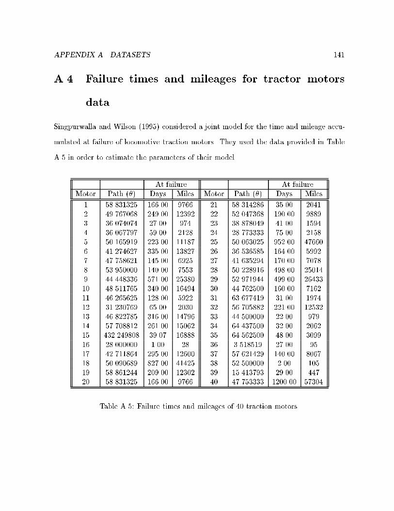
APPENDIX A. DATASETS 141
A.4 Failure times and mileages for tractor motors
data
Singpurwalla and Wilson (1995) considered a joint model for the time and mileage accu-
mulated at failure of locomotive traction motors. They used the data provided in Table
A.5 in order to estimate the parameters of their model.
At failure At failure
Motor Path (�) Days Miles Motor Path (�) Days Miles
1 58.831325 166.00 9766 21 58.314286 35.00 20412 49.767068 249.00 12392 22 52.047368 190.00 9889
3 36.074074 27.00 974 23 38.878049 41.00 15944 36.067797 59.00 2128 24 28.773333 75.00 21585 50.165919 223.00 11187 25 50.063025 952.00 47660
6 41.274627 335.00 13827 26 36.536585 164.00 59927 47.758621 145.00 6925 27 41.635294 170.00 70788 53.950000 140.00 7553 28 50.228916 498.00 250149 44.448336 571.00 25380 29 52.971944 499.00 2643310 48.511765 340.00 16494 30 44.762500 160.00 7162
11 46.265625 128.00 5922 31 63.677419 31.00 197412 31.230769 65.00 2030 32 56.705882 221.00 1253213 46.822785 316.00 14796 33 44.500000 22.00 97914 57.708812 261.00 15062 34 64.437500 32.00 2062
15 432.249808 39.07 16888 35 64.562500 48.00 3099
16 28.000000 1.00 28 36 3.518519 27.00 9517 42.711864 295.00 12600 37 57.621429 140.00 8067
18 50.090689 827.00 41425 38 52.500000 2.00 10519 58.861244 209.00 12302 39 15.413793 29.00 447
20 58.831325 166.00 9766 40 47.753333 1200.00 57304
Table A.5: Failure times and mileages of 40 traction motors.
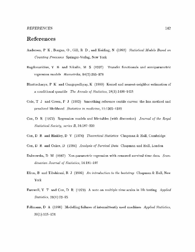
REFERENCES 142
References
Andersen, P. K., Borgan, O., Gill, R. D., and Keiding, N. (1993). Statistical Models Based on
Counting Processes. Springer-Verlag, New York.
Bagdonavi�cius, V. B. and Nikulin, M. S. (1997). Transfer functionals and semiparametric
regression models. Biometrika, 84(2):365{378.
Bhattacharya, P. K. and Gangopadhyay, K. (1990). Kernel and nearest-neighbor estimation of
a conditional quantile. The Annals of Statistics, 18(3):1400{1415.
Cole, T. J. and Green, P. J. (1992). Smoothing reference centile curves: the lms method and
penalized likelihood. Statistics in medicine, 11:1305{1319.
Cox, D. R. (1972). Regression models and life-tables (with discussion). Journal of the Royal
Statistical Society, series B, 34:187{220.
Cox, D. R. and Hinkley, D. V. (1974). Theoretical Statistics. Chapman & Hall, Cambridge.
Cox, D. R. and Oakes, D. (1984). Analysis of Survival Data. Chapman and Hall, London.
Dabrowska, D. M. (1987). Non-parametric regression with censored survival time data. Scan-
dinavian Journal of Statistics, 14:181{197.
Efron, B. and Tibshirani, R. J. (1993). An introduction to the bootstrap. Chapman & Hall, New
York.
Farewell, V. T. and Cox, D. R. (1979). A note on multiple time scales in life testing. Applied
Statistics, 28(1):73{75.
Follmann, D. A. (1990). Modelling failures of intermittently used machines. Applied Statistics,
39(1):115{124.
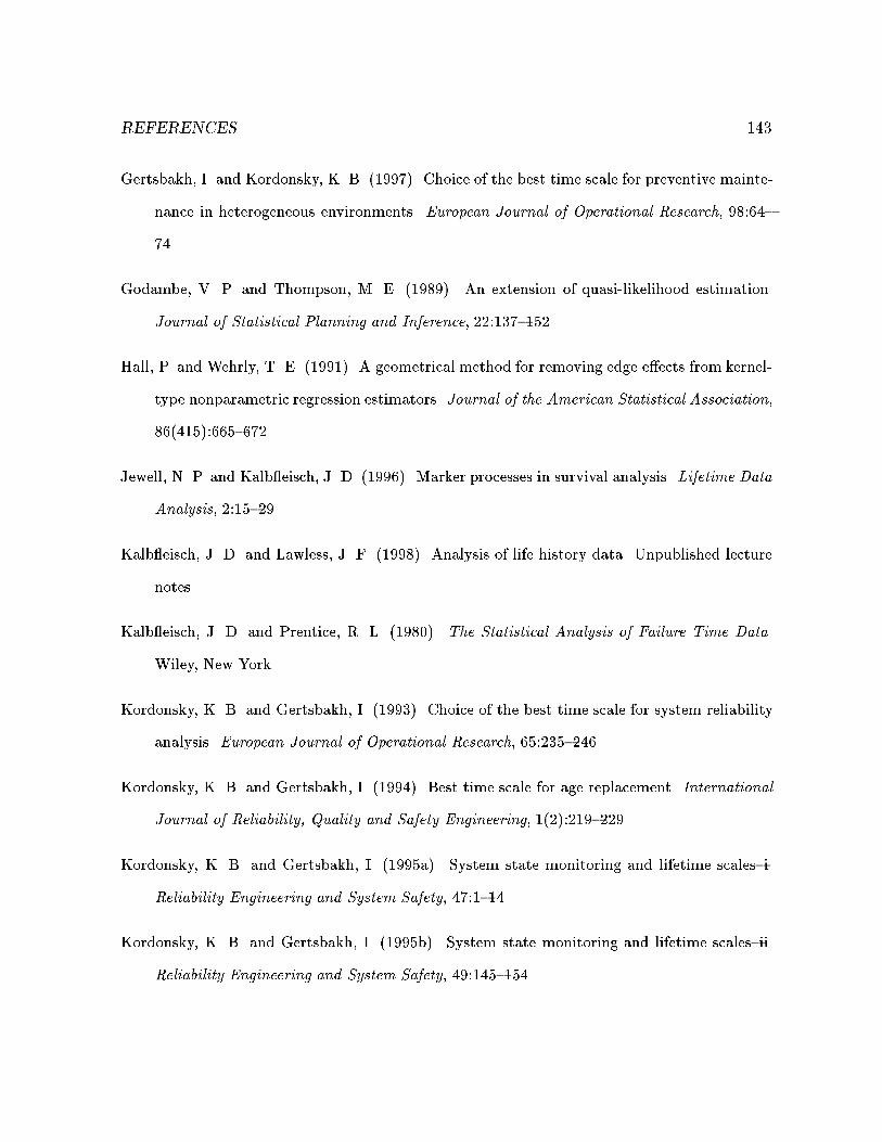
REFERENCES 143
Gertsbakh, I. and Kordonsky, K. B. (1997). Choice of the best time scale for preventive mainte-
nance in heterogeneous environments. European Journal of Operational Research, 98:64{
74.
Godambe, V. P. and Thompson, M. E. (1989). An extension of quasi-likelihood estimation.
Journal of Statistical Planning and Inference, 22:137{152.
Hall, P. and Wehrly, T. E. (1991). A geometrical method for removing edge e�ects from kernel-
type nonparametric regression estimators. Journal of the American Statistical Association,
86(415):665{672.
Jewell, N. P. and Kalb eisch, J. D. (1996). Marker processes in survival analysis. Lifetime Data
Analysis, 2:15{29.
Kalb eisch, J. D. and Lawless, J. F. (1998). Analysis of life history data. Unpublished lecture
notes.
Kalb eisch, J. D. and Prentice, R. L. (1980). The Statistical Analysis of Failure Time Data.
Wiley, New York.
Kordonsky, K. B. and Gertsbakh, I. (1993). Choice of the best time scale for system reliability
analysis. European Journal of Operational Research, 65:235{246.
Kordonsky, K. B. and Gertsbakh, I. (1994). Best time scale for age replacement. International
Journal of Reliability, Quality and Safety Engineering, 1(2):219{229.
Kordonsky, K. B. and Gertsbakh, I. (1995a). System state monitoring and lifetime scales{i.
Reliability Engineering and System Safety, 47:1{14.
Kordonsky, K. B. and Gertsbakh, I. (1995b). System state monitoring and lifetime scales{ii.
Reliability Engineering and System Safety, 49:145{154.
REFERENCES 144
Kordonsky, K. B. and Gertsbakh, I. (1997a). Fatigue crack monitoring in parallel time scales.
Proceedings of the ESREL conference, Lisbon, Portugal.
Kordonsky, K. B. and Gertsbakh, I. (1997b). Multiple time scales and the lifetime coe�cient
of variation: Engineering applications. Lifetime Data Analysis, 2:139{156.
Lawless, J. F. (1982). Statistical Models and Methods for Lifetime Data. Wiley, New York.
Lawless, J. F., Hu, J., and Cao, J. (1995). Methods for the estimation of failure distributions
and rates from automobile warranty data. Lifetime Data Analysis, 1:227{240.
Lejeune, M. G. and Sarda, P. (1988). Quantile regression: a nonparametric approach. Compu-
tational Statistics & Data Analysis, 6:229{239.
Lin, D. Y. and Ying, Z. (1995). Semiparametric inference for the accelerated life model with
time-dependent covariates. Journal of Statistical Planning and Inference, 44:47{63.
McCullagh, P. and Nelder, J. A. (1989). Generalized linear models. Chapman and Hall, London,
2nd edition.
Meeker, W. Q. and Escobar, L. A. (1998). Statistical methods for reliability data. Wiley, New
York.
Murthy, D. N. P., Iskandar, B. P., and Wilson, R. J. (1995). Two dimensional failure free
warranty policies: Two dimensional point process models. Operations Research, 43:356{
366.
Nelson, W. (1990). Accelerated Testing: Statistical Models, Test Plans and Data Analyses.
Wiley, New York.
Oakes, D. (1995). Multiple time scales in survival analysis. Lifetime Data Analysis, 1:7{18.

REFERENCES 145
Press, W. H., Teukolsky, S. A., Vetterling, W. T., and Flannery, B. P. (1992). Numerical recipes
in C: the art of scienti�c computing. Cambridge University Press, Cambridge, 2nd edition.
Reinertsen, R. (1996). Residual life of technical systems; diagnosis, prediction and life extension.
Reliability Engineering and System Safety, 54:23{34.
Robins, J. and Tsiatis, A. A. (1992). Semiparametric estimation of an accelerated failure time
model with time-dependent covariates. Biometrika, 79(2):311{319.
Schijve, J. and Jakobs, F. (1960). Program-fatigue test on notched light alloy specimen of 2024
and 7075 material. Technical Report M 2070, National Res. Inst., Amsterdam.
Singpurwalla, N. D. (1995). Survival in dynamic environments. Statistical Science, 10(1):86{
103.
Singpurwalla, N. D. and Wilson, S. (1993). The warranty problem: its statistical and game
theoretic aspects. SIAM Review, 35:17{42.
Singpurwalla, N. D. and Wilson, S. P. (1995). Life distributions indexed by multiple scales.
Unpublished manuscript.