multiple tests, bonferroni correction, fdr
TRANSCRIPT

Multiple tests, Bonferroni correction, FDR
Joe Felsenstein
Department of Genome Sciences and Department of Biology
Multiple tests, Bonferroni correction, FDR – p.1/14

Multiple tests
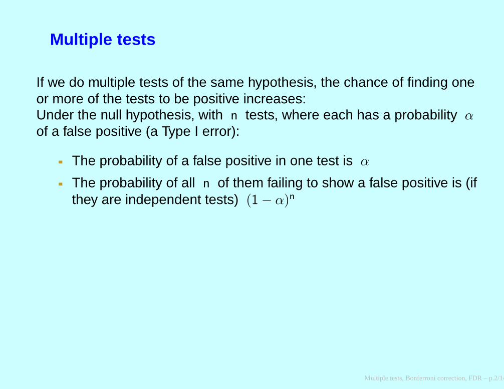
If we do multiple tests of the same hypothesis, the chance of finding oneor more of the tests to be positive increases:Under the null hypothesis, with n tests, where each has a probability αof a false positive (a Type I error):
The probability of a false positive in one test is α
Multiple tests, Bonferroni correction, FDR – p.2/14
Multiple tests
If we do multiple tests of the same hypothesis, the chance of finding oneor more of the tests to be positive increases:Under the null hypothesis, with n tests, where each has a probability αof a false positive (a Type I error):
The probability of a false positive in one test is α
The probability of all n of them failing to show a false positive is (ifthey are independent tests) (1 − α)n
Multiple tests, Bonferroni correction, FDR – p.2/14

Multiple tests
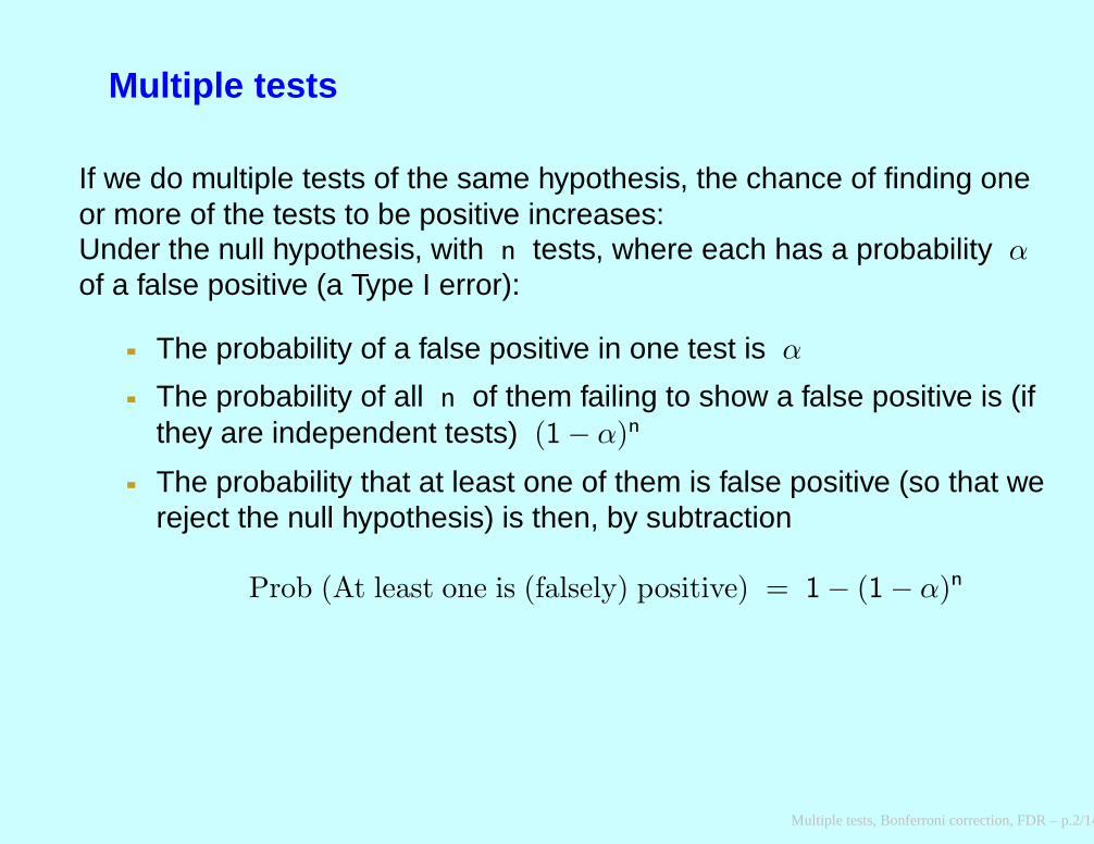
If we do multiple tests of the same hypothesis, the chance of finding oneor more of the tests to be positive increases:Under the null hypothesis, with n tests, where each has a probability αof a false positive (a Type I error):
The probability of a false positive in one test is α
The probability of all n of them failing to show a false positive is (ifthey are independent tests) (1 − α)n
The probability that at least one of them is false positive (so that wereject the null hypothesis) is then, by subtraction
Prob (At least one is (falsely) positive) = 1 − (1 − α)n
Multiple tests, Bonferroni correction, FDR – p.2/14
Multiple tests
If we do multiple tests of the same hypothesis, the chance of finding oneor more of the tests to be positive increases:Under the null hypothesis, with n tests, where each has a probability αof a false positive (a Type I error):
The probability of a false positive in one test is α
The probability of all n of them failing to show a false positive is (ifthey are independent tests) (1 − α)n
The probability that at least one of them is false positive (so that wereject the null hypothesis) is then, by subtraction
Prob (At least one is (falsely) positive) = 1 − (1 − α)n
Multiple tests, Bonferroni correction, FDR – p.2/14

Probability of a false positive with multiple tests
So the probability of a false positive can get fairly high:
Number of tests Prob(false positive)1 0.052 0.09753 0.1426254 0.18549385 0.2262
10 0.4012615 0.536720 0.641550 0.9231
100 0.9941
Multiple tests, Bonferroni correction, FDR – p.3/14
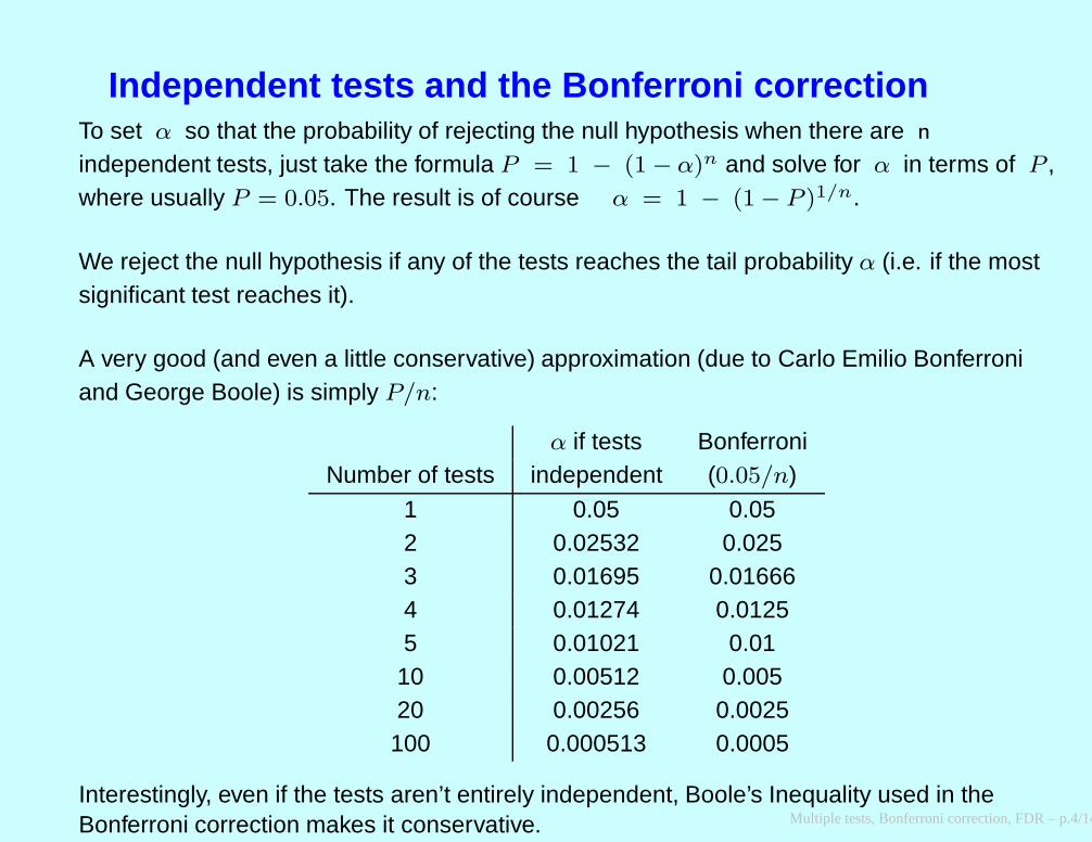
Independent tests and the Bonferroni correctionTo set α so that the probability of rejecting the null hypothesis when there are n
independent tests, just take the formula P = 1 − (1 − α)n and solve for α in terms of P ,where usually P = 0.05. The result is of course α = 1 − (1 − P )1/n.
We reject the null hypothesis if any of the tests reaches the tail probability α (i.e. if the mostsignificant test reaches it).
A very good (and even a little conservative) approximation (due to Carlo Emilio Bonferroniand George Boole) is simply P/n:
α if tests BonferroniNumber of tests independent (0.05/n)
1 0.05 0.052 0.02532 0.0253 0.01695 0.016664 0.01274 0.01255 0.01021 0.01
10 0.00512 0.00520 0.00256 0.0025100 0.000513 0.0005
Interestingly, even if the tests aren’t entirely independent, Boole’s Inequality used in theBonferroni correction makes it conservative. Multiple tests, Bonferroni correction, FDR – p.4/14

Type I and Type II errors and all that
If we know the alternative hypothesis and how the data are distributed onit, you can calculate the probability of concluding that H0 is true or false,and the probability that H1 is true of false:
type IIerror
type I error (α)
power (β)
we accept we rejectH H0 0
H
H0
1
0or whatever
The probability of (correctly) rejecting the null hypothesis is the power,called β (blue area in figure).
A type I error is false rejecting the null hypothesis (red in the figure). AType II error is false rejecting the alternative hypothesis (orange).
Multiple tests, Bonferroni correction, FDR – p.5/14

Sensitivity, specificity, FPR, TPR
Truth is:We conclude: H1 H0
H1 TP FPH0 FN TN
False Positive Rate: the fraction of cases which appear to have H1
true among those which actually have H0 true (=?)
Multiple tests, Bonferroni correction, FDR – p.6/14

Sensitivity, specificity, FPR, TPR
Truth is:We conclude: H1 H0
H1 TP FPH0 FN TN
False Positive Rate: the fraction of cases which appear to have H1
true among those which actually have H0 true (=?)
FPR = FP/(FP + TN) (= 1 − specificity = α)
Multiple tests, Bonferroni correction, FDR – p.6/14

Sensitivity, specificity, FPR, TPR
Truth is:We conclude: H1 H0
H1 TP FPH0 FN TN
False Positive Rate: the fraction of cases which appear to have H1
true among those which actually have H0 true (=?)
FPR = FP/(FP + TN) (= 1 − specificity = α)
True Positive Rate: the fraction of apparent positives among truepositives (=?)
TPR = TP/(TP + FN) (= sensitivity = power = β)
Multiple tests, Bonferroni correction, FDR – p.6/14

The False Discovery Rate
FDR = FP/(FP + TP )
Contrary to what you will hear, it is for a different case:
Bonferroni: Testing the same hypothesis many times, or manydifferent ways. (Some tests may be much less powerful thanothers). If even one test really shows that the null hypothesis iswrong, then it is dead.
FDR: We are testing many hypotheses (in a similar way). We wantto know which ones are likely to be true.
The idea of the considering the FDR is to see what the fraction of falsepositives might be among among all those that appear to be true.
Multiple tests, Bonferroni correction, FDR – p.7/14

Holm’s method
Another way of choosing promising hypotheses is to accept the mostsignificant test, then the next most significant, and so on until one fails.
Holm showed that the proper way to do this, to have a probability α ofaccepting any test when the null hypothesis is actually true is, say if therewere 120 tests of different hypotheses:
Test the one with the smallest P value against α/120
Test the one with the next smallest P value against α/119
Test the one with the next smallest P value against α/118
... and so on, until one is not significant.
This is an alternative to the FDR machinery.
Multiple tests, Bonferroni correction, FDR – p.8/14

The ROC Curve
In the (mostly unrealistic) cases where we know the distributions of dataunder the null hypothesis and the alternative hypothesis, we can plot theTPR as a function of the FPR, for different P values we might use. Forhistorical reasons (radar in World War II) this is called the ReceiverOperating Characteristic curve:
FPR
TPR
0
1
0 1α
β
Multiple tests, Bonferroni correction, FDR – p.9/14

The ROC Curve and the type I and type II errors
Here is a diagram showing plotting the fraction of True Positives againstthe power (which we could do if we knew everything):
0 10
1
H0 H1
β
α
β
α
Multiple tests, Bonferroni correction, FDR – p.10/14

The ROC Curve and the type I and type II errors
Here is a diagram showing plotting the fraction of True Positives againstthe power (which we could do if we knew everything):
0 10
1
H0 H1
β
α
H0 H1
β
α
β
α
Multiple tests, Bonferroni correction, FDR – p.10/14

The ROC Curve and the type I and type II errors
Here is a diagram showing plotting the fraction of True Positives againstthe power (which we could do if we knew everything):
0 10
1
H0 H1
β
α
H0 H1
β
α
H0 H1
β
α
β
α
Multiple tests, Bonferroni correction, FDR – p.10/14

The ROC Curve – an example
If the null is Normal(0,1) and the alternative is Normal(1,1), and the data isone observation, here is the ROC:
0.0 0.2 0.4 0.6 0.8 1.0
0.0
0.2
0.4
0.6
0.8
1.0
FPR
TP
R
Multiple tests, Bonferroni correction, FDR – p.11/14

The distribution of P is flat under the null hypothesis
The probability that P just reaches the 0.05 level is (duh) 0.05.
Multiple tests, Bonferroni correction, FDR – p.12/14

The distribution of P is flat under the null hypothesis
The probability that P just reaches the 0.05 level is (duh) 0.05.
The probability that P just reaches the 0.2 level is 20%.
Multiple tests, Bonferroni correction, FDR – p.12/14

The distribution of P is flat under the null hypothesis
The probability that P just reaches the 0.05 level is (duh) 0.05.
The probability that P just reaches the 0.2 level is 20%.
And similarly for any other value.
Multiple tests, Bonferroni correction, FDR – p.12/14

The distribution of P is flat under the null hypothesis
The probability that P just reaches the 0.05 level is (duh) 0.05.
The probability that P just reaches the 0.2 level is 20%.
And similarly for any other value.
So the distribution of the P if the null hypothesis is true is a flat(rectangular) distribution between 0 and 1:
0 1P
Multiple tests, Bonferroni correction, FDR – p.12/14

Storey’s way of calculating the FDR
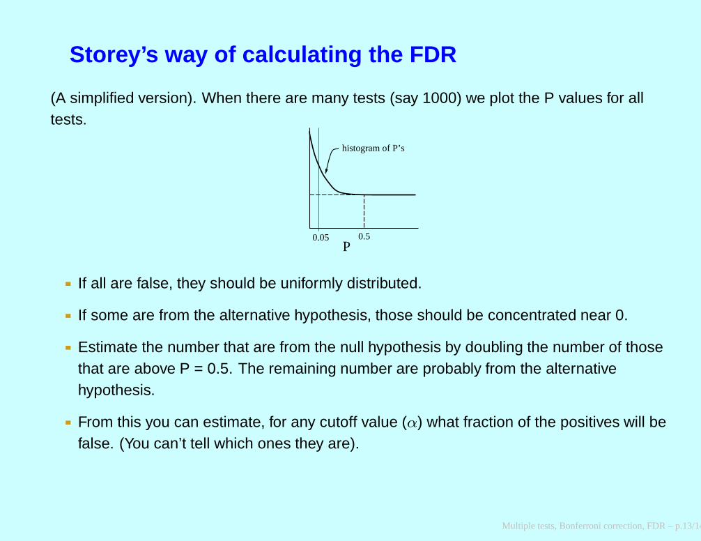
(A simplified version). When there are many tests (say 1000) we plot the P values for alltests.
0.05P
0.5
histogram of P’s
If all are false, they should be uniformly distributed.
Multiple tests, Bonferroni correction, FDR – p.13/14

Storey’s way of calculating the FDR
(A simplified version). When there are many tests (say 1000) we plot the P values for alltests.
0.05P
0.5
histogram of P’s
If all are false, they should be uniformly distributed.
If some are from the alternative hypothesis, those should be concentrated near 0.
Estimate the number that are from the null hypothesis by doubling the number of thosethat are above P = 0.5. The remaining number are probably from the alternativehypothesis.
Multiple tests, Bonferroni correction, FDR – p.13/14
Storey’s way of calculating the FDR
(A simplified version). When there are many tests (say 1000) we plot the P values for alltests.
0.05P
0.5
histogram of P’s
If all are false, they should be uniformly distributed.
If some are from the alternative hypothesis, those should be concentrated near 0.
Estimate the number that are from the null hypothesis by doubling the number of thosethat are above P = 0.5. The remaining number are probably from the alternativehypothesis.
From this you can estimate, for any cutoff value (α) what fraction of the positives will befalse. (You can’t tell which ones they are).
Multiple tests, Bonferroni correction, FDR – p.13/14

Storey’s way of calculating the FDR
(A simplified version). When there are many tests (say 1000) we plot the P values for alltests.
0.05P
0.5
histogram of P’s
If all are false, they should be uniformly distributed.
If some are from the alternative hypothesis, those should be concentrated near 0.
Estimate the number that are from the null hypothesis by doubling the number of thosethat are above P = 0.5. The remaining number are probably from the alternativehypothesis.
From this you can estimate, for any cutoff value (α) what fraction of the positives will befalse. (You can’t tell which ones they are).
For example, if out of T tests A are above 0.5, another A are estimated to be uniformlydistributed below 0.5. Below 0.05 will be A/10. So the FDR is A/10 divided by thenumber you see below 0.05, which we could call B.
Multiple tests, Bonferroni correction, FDR – p.13/14

If you’re a Bayesian, however ...
... you don’t need any of the above, just use your priors and theposteriors.
Multiple tests, Bonferroni correction, FDR – p.14/14