multiple analysis of series for homogenization ( m a s h ... · preface of version mashv3.02 the...

Multiple Analysis of Series for Homogenization

( M A S H v3.02)

Tamás Szentimrey

Hungarian Meteorological Service

H-1525, P.O. Box 38, Budapest, Hungary

e-mail: [email protected]

I. MATHEMATICAL BASIS ..…………........……………................................ 5

II. THE STRUCTURE OF PROGRAM SYSTEM ....................................... 21

III. THE MASH SYSTEM .............................….................…............................. 23

IV. THE SAM SYSTEM (Seasonal Application of MASH) .….…............ 27

V. EXAMPLE FOR APPLICATION OF MASH SYSTEM ................... 34

VI. EXAMPLE FOR APPLICATION OF SAM SYSTEM ....................... 43

VII. HOMOGENIZATION OF DAILY DATA .............................................. 53

ANNEX: SOME DEVELOPMENTS FOR AUTOMATION ………...…... 64

PREFACE of Version MASHv3.02

The MASH procedure was developed originally for homogenization of monthly series. It is a relative method and depending on the distribution of examined meteorological element additive (e.g. temperature) or multiplicative (e.g. precipitation) model can be applied. In the earlier program system MASHv2.03 the following subjects were elaborated for monthly series: series comparison, break point (changepoint) and outlier detection, correction of series, missing data complementing, automatic usage of meta data and last but not least a verification procedure to evaluate the homogenization results.

The next version MASHv3.01 was developed for homogenization of daily data furthermore for quality control of daily data and missing data complementing. During the procedure normal distribution and additive model were assumed for daily data that are appropriate for temperature, pressure etc. elements.

The new version MASHv3.02 is extended also for homogenization of daily precipitation data. The procedure developed for daily data is in accordance with the multiplicative (or cumulative) model that is assumed for monthly precipitation sum data. Quality control of daily data and missing data complementing are also performed during the procedure. Remark 1

The program system for homogenization of monthly series was not changed so the manual of MASH2.03 can be used invariably (pages 1-52). Only exception is the type of usable coordinates that were changed for filambda type, because perhaps it is more general (see pages: 24, 29, 35, 43). The structure of program system (page 21) is completed with the daily data part. The description of procedure for daily data can be found from page 53. Remark 2 In the Annex (page 64) some new developments for automation are enclosed. These ‘user friendly’ procedures make the homogenization easier for the users.

1

PREFACE of Version MASHv2.03

The MASH method was developed in the Hungarian Meteorological Service (see References). It is a relative homogeneity test procedure that does not assume the reference series are homogeneous. Possible break points and shifts can be detected and adjusted through mutual comparisons of series within the same climatic area. The candidate series is chosen from the available time series and the remaining series are considered as reference series. The role of series changes step by step in the course of the procedure. Depending on the climatic elements, additive or multiplicative models are applied. The second case can be transformed into the first one by logarithmization. Several difference series are constructed from the candidate and weighted reference series. The optimal weighting is determined by minimizing the variance of the difference series, in order to increase the efficiency of the statistical tests. Providing that the candidate series is the only common series of all the difference series, break points detected in all the difference series can be attributed to the candidate series. A new multiple break points detection procedure has been developed which takes the problem of significance and efficiency into account. The significance and the efficiency are formulated according to the conventional statistics related to type one and type two errors, respectively. This test obtains not only estimated break points and shift values, but the corresponding confidence intervals as well. The series can be adjusted by using the point and interval estimates.

Since a MASH program system has been developed for the PC, the application of this method is relatively easy, with emphasis on GAME of MASH (see program MASHGAME.BAT), which is a playful version of MASH procedure for homogenization. This version can be developed towards the automation (see program MASHGAUT.BAT). Some developments are connected with special problems of the homogenization of climatic time series. One of them is the relation of monthly, seasonal and annual series. The problem arises from the fact, that the signal to noise ratio is probably less in case of monthly series than in case of derived seasonal or annual ones. Consequently the inhomogeneity can be detected easier at the derived series although we intend to adjust the monthly series (see the SAM system). Another problem is connected with the usage of Meta Data in the course of homogenization procedure. The developed version of MASH system makes possible to use the meta data information - in particular the probable dates of break points - automatically. The new version includes a new transformation procedure as well, which has been developed for the multiplicative model on purpose to solve the problem arising from the values coming near to zero.

A new part of MASH system is a verification procedure (MASHVERI.BAT) which makes possible to evaluate the actual or the final stage of the homogenization. We think the verification is an important part of the topic of homogenization since all over the world there are a lot of so called homogenized series however their reliability sometimes is doubtful. The basic conception of the verification procedure is that the confidence in the homogenized series may be increased by the joint comparative mathematical examination of the original and the homogenized series systems.

The last development is connected with certain automation of the procedures (see programs: MASHGAUH.BAT, SAMTEST.BAT).

2

(MOTTO)

PROBLEM of HOMOGENIZATION

Basis: DATA

Tools:

MATHEMATICS : abstract formulation

META DATA : historical, climatological information

SOFTWARE : automation

SOLUTION = MATHEMATICS + META DATA + SOFTWARE

(i) without SOFTWARE:

MATHEMATICS + META DATA = THEORY WITHOUT BENEFIT

(ii) without META DATA:

MATHEMATICS + SOFTWARE = GAMBLING

(iii) without MATHEMATICS:

META DATA + SOFTWARE = “STONE AGE” + “BILL GATES”

3

BASIC PRINCIPLES of MASH Procedure

- Relative homogeneity test procedure.

- Step by step procedure: the role of series (candidate or reference series)

changes step by step in the course of the procedure.

- Additive or cumulative model can be used depending on the climate

elements.

- Monthly, seasonal or annual time series can be homogenized.

- In case of having monthly series for all the 12 months, the monthly,

seasonal and annual series can be homogenized together.

(SAM procedure: Seasonal Application of MASH)

- The daily inhomogeneities can be derived from the monthly ones.

- META DATA (probable dates of break points) can be used

automatically.

- The actual or the final stage of the homogenization can be verified.

PROGRAMMED STATISTICAL PROCEDURE

(SOFTWARE: MASHv2.03)

EXAMPLE. Let us assume that there is a difficult stochastic problem.

In case of having relatively few statistical information:

- an intelligent man is possibly able to solve the problem, but it is time-

consuming;

- the solution of the problem can not be programmed.

In case of increasing the amount of statistical information:

- one is unable to discuss and evaluate all the information,

- but then the solution of the problem can be programmed. (CHESS!!)

AIM, REQUIREMENT

- Development of mathematical methodology in order to increase the

amount of statistical information.

- Development of algorithms for optimal using of both the statistical and

the ‘meta data’ information.

4

THE MAIN CLIMATOLOGICAL AND STATISTICAL PROBLEMS

Modelling of the stochastic relationship between data series:

additive model, cumulative (multiplicative) model depending on climate elements,

distribution of series elements.

Modelling of "inhomogeneity": break points, shifts, outliers etc..

Comparison of the examined series (Relative Test): methods for multiple

comparison of the candidate series with more reference series; selection for

"good" reference series systems, weighting of reference series, estimation of

weighting factors. Multiple Comparison by Optimum Interpolation.

Missing values: methods for closing gaps in the series.

Break points detection:

mathematical formalization according to the statistical conventions:

- first kind error ( significance )

- second kind error ( efficiency ),

point estimation and interval estimation (confidence interval),

procedure for multiple break points and outliers detection.

Correction (adjusting) of candidate series:

separation of the detected break points and outliers for the candidate series,

point estimation, interval estimation (confidence interval) for the shifts. Relation of monthly series, seasonal series, annual series:

SAM (Seasonal Application of MASH).

Meta Data: automatic using of station history. Automation: interactive, automatic procedures for homogenization.

Verification: procedure to evaluate the homogenization results.

5

I. THE MATHEMATICAL BASIS OF ‘MASH’ PROCEDURE

(draft version)

1. STATISTICAL MODELLING

1.1 Additive Model (for example temperature)

Examined series

)(tX j += )(tC j )(tIH j )(tjε+ ( ).,n,, t,N ,,j …=…= 21;21

C : climate change; IH : inhomogeneity, ε : noise 1.2 Multiplicative Model (for example monthly or seasonal precipitation)

Examined series

)(*tX j ⋅= )(*

tC j )(*tIH j )(*

tjε⋅ ( ).,n,, t,N ,,j …=…= 21;21

*

C : climate change; *IH : inhomogeneity, *ε : noise

Logarithmization for Additive Model

)(tX j += )(tC j )(tIH j )(tjε+ ( ).,n,, t,N ,,j …=…= 21;21

where

)(ln)( *tXtX jj = , )(ln)( *

tCtC jj = ,

)(ln)( *tIHtIH jj = , )(ln)( *

tt jj εε =

Problem

If )(*tX j values are near or equal to 0 .

This problem can be solved by a Transformation Procedure which increases slightly the little values. Consequently the Multiplicative Model can be transformed into the Additive One.

6

2. MULTIPLE COMPARISON OF THE EXAMINED SERIES

Candidate series and its inhomogeneity: )(tX c , )(tIH c { }Nc ,...,2,1∈

Set of indexes of reference series: { }NRc ,...,2,1⊂ ( ))()(if, tcCtiCRi c ≈∈

Optimal Difference Series belonging to the subset cm

c RR ⊆)( )( 12,..,1 −= cRm

)numerosity:(

)()()()(

)(tXwtXtZ i

Ri

icm

cm

c

⋅−= ∑∈

, where 1=∑ iw , 0≥iw

and =)V( )(mcZ =)( Variance )(m

cZw

minimum

Result:

)()()()(

)(tIHwtIHtZ i

Riic

mc

mc

⋅−= ∑∈

=+ )()(tδ

mc )()( )( tIHtIH m

cRc − )()(tδ

mc+

Example:

If =)V )(mcZ( 0)Variance( )( =m

cδ and 0)()( ≡tIH mcR

then )()()(tIHtZ c

mc ≡

Optimal Difference Series System: 2,12,....,1,)( **)( ≥Μ

−Μ ⊂∈ cRm

c mtZ

(i) )()(tZ

mc : Optimal Difference Series belonging to subset )(m

cR (for

efficiency)

(ii) ∅=Μ∈

)(

*

mc

m

RI (for identification of inhomogeneity of candidate

series)

(iii) **

minimum))Variance((maximum )(

ΜΜ∈

=mc

m

Z (for efficiency)

(iv) If (i), (ii), (iii) are fulfilled then let *Μ be minimal too! (for efficiency)

7

3. EXAMINATION OF DIFFERENCE SERIES 3.1 Break Points Detection

Difference series: )()()( ttIHtZ δ+= ( ).,n,, t …= 21

)(tIH ......

1 1P LP n

The real break points (to the left) : { }nPPP L <<<<≤ .....1 21

BASIC POSTULATES FOR THE DECISION METHODS ( FORMALIZATION )

The detected break points:

<<<<≤∧

∧∧∧nPPP L.....1 21

(i) Type one error (significance)

There exists such a lP∧

:

interval )( 11 +

∧∧

ll- P,P I { }LPPP <<< .....set 21 ∅=

homogeneous

)(tIH

1−

∧

lP lP∧

1+

∧

lP

We have to intend to give the probability of type one error, i.e. the significance level!

(ii) Type two error (efficiency)

There exists such a real break point that we could not detect. As much as possible!

8

3.2 Significant Procedure for Break Points Detection

Inhomogeneity measure for all the intervals Statistics: [ ]( ) 0,INH ≥lk ∀ lk , : nlk ≤<≤1

and [ ]( )ji ,INH ≤ [ ]( )lk ,INH , if [ ]ji , ⊆ [ ]lk ,

Test Statistic of difference series

The inhomogeneity of difference series )(tZ can be characterized by the

Test Statistic: =TS [ ]( )n,1INH

The critical value ( α ) ( by Monte Carlo Method )

( ) =|> shomogeneou)(ifTSP tZα sig. level ( )01.0,05.0,1.0=

Test Statistic can be compared to the critical value and in case of homogeneity it

should be less, on the given significance level.

PROPERTIES OF THE DETECTING PROCEDURE

(FOR THE PURPOSE OF SIGNIFICANCE AND EFFICIENCY)

If the detected break points:

<<<<≤∧∧∧∧

nPPP L.....1 21 , then

<≤

∧∧

+=∧

α)( ]( 1

1,...,1

INHmaximum ll-

Ll

P,P

+

∧∧

=∧

)( ]( 11

,...,1

INHminimum ll-

Ll

P,P

i.e. on the given significance level:

- the intervals ]( 11 +

∧∧

ll- P,P are not homogeneous, consequently the detected

break points lP∧

are not superfluous,

- the intervals ]( 1 ll- P,P∧∧

can be accepted to be homogeneous.

9

Confidence Intervals

Confidence intervals also can be given for the break points on the

confidence level (1-sig. level): lΙ ∧

= Ll ,....,1

3.3 Estimation of Shifts

Point estimation; Confidence intervals for the shifts

4. EVALUATION OF HOMOGENEITY OF CANDIDATE SERIES )(tXc

Based on the Test Statistics (TS) belonging to the Optimal Difference Series:

)()(tZ

mc )( 12,..,1 −= cR

m

5. CORRECTION OF CANDIDATE SERIES )(tX c

Based on the examination of the Optimal Difference Series System:

−Μ∈ ⊂ 12,....,1,)( *)( cRm

c mtZ , 2* ≥Μ

BASIC PRINCIPLE OF BREAK POINT DETECTION FOR CANDIDATE SERIES Let us assume, that

)(mP∧

)( *Μ∈m : detected Break Points, )(mΙ )( *Μ∈m : Confidence Intervals

belonging to the Optimal Difference Series )()(tZ

mc )( *Μ∈m , AND

∅Ι ≠Μ∈

)(

*

m

m

I as well as ∀ ∈∧

)(mP)(

*

m

m

ΙΜ∈

I

DECISION

The „most probable” )(mP∧

is a Break Point of the Candidate Series )(tXc .

10

6. USING OF META DATA (Meta Data: probable dates of break points)

BASIC PRINCIPLE OF BREAK POINT DETECTION BY USING OF META DATA Candidate series and its Meta Data:

)(tX c , { }nDDDc

Kcc

cc

<<<<≤=∆ )()(2

)(1 ....1

Optimal Difference Series System: )()(tZ

mc , *Μ∈m , 2* ≥Μ

Let us assume, that

)(mP∧

)( *Μ∈m : detected Break Points, )(mΙ )( *Μ∈m : Confidence Intervals

belonging to the Optimal Difference Series )()(tZ

mc )( *Μ∈m , AND

∅Ι ≠Μ∈

)(

*

m

m

I as well as ∀ ∈∧

)(mP)(

*

m

m

ΙΜ∈

I

BASIC DECISION RULE

(i) If ∅Ι ≠

= ∆

Μ∈c

m

m

II )(

*:Q

The „most probable” )(cD Q∈ is a Break Point of the Candidate Series )(tXc .

(Break Point: Meta Data)

(ii) If ∅Ι =

∆

Μ∈c

m

m

II )(

* but ∅Ι ≠

∆

Μ∈c

m

m

IU )(

*

No Decision.

(iii) If ∅Ι =

∆

Μ∈c

m

m

IU )(

*

The „most probable” )(mP∧

is a Break Point of the Candidate Series )(tXc .

(Break Point: is not Meta Data, but „undoubtful”)

11

7. EVALUATION OF META DATA

(Meta Data: probable dates of break points) THE QUALITY OF META DATA CAN BE VERIFIED BY STATISTICAL TESTS!!!

For example: the problem of Missing Meta Data??

In Practice: the statistical Test Results are often verified with the Meta Data.

BUT: the question may be turned round! Examined series and their Meta Data

)(tX j , { }nDDD j

K

jj

j j<<<<≤=∆ )()(

2)(

1 ....1 ( ).,N,, j …= 21

Candidate series and its Meta Data: )(tXc , c∆ { }Nc ,...,2,1∈

Optimal Difference Series belonging to the subset cm

c RR ⊆)( :

)()()()(

)(tXwtXtZ i

Riic

mc

mc

⋅−= ∑∈

( ))()()(

tXtXw icRi

im

c

−⋅= ∑∈

)()(

tZw ciRi

im

c

⋅= ∑∈

Transformation of Difference Series )(tZci

{ }nDDDic

Kicic

icicic

<<<<≤== ∨∨∨∨

∨∆∆∆ )()(

1)(

1 ...1U

≤<−

=≤<−

≤≤−

=

∨∨

∨∨∨

−∨∨

−

∨∨

∨∨ntDnDZtZ

KkDtDDDZtZ

DtDZtZ

tZ

icK

icKcici

icic

kic

kic

kic

kcici

iciccici

ci

icic

)()(

)()(1

)()(1

)(1

)(1

if,],()(

),...,2(if,],()(

1if,],1[)(

)(~

baZci , : average of )(tZci above the interval ba, .

Transformed Optimal Difference Series belonging to the subset cm

c RR ⊆)( :

)(~ )(

tZm

c )(~

)(

tZw ciRi

im

c

⋅= ∑∈

)( 12,..,1 −= cRm

are homogeneous if the inhomogeneities can be explained by the Meta Data!

EVALUATION OF META DATA: Based on the Test Statistics (TS) belonging to the

Transformed Optimal Difference Series )(~ )(

tZm

c .

12

8. SEASONAL APPLICATION OF MASH (SAM)

Monthly difference series: )()(tZ

k ( ).,K,, k …= 21

Expectations and Variances: =))(E( )(tZ

k )()(tIH

k , )V( )(kZ

Seasonal mean difference series: =)(tZ ∑=

K

k

ktZ

K 1

)( )(1

Expectation and Variance: =))(E( tZ =)(tIH

__

∑=

K

k

ktIH

K 1

)( )(1

, )V(Z

The test results after the Homogenization of monthly series

0H : 0)()( ≡tIHk ( ).,K,, k …= 21 can be accepted.

BUT! (sometimes) 0H : 0)(__

≡tIH can not be accepted!

The reason of the problem The efficiency of test depends on the signal to noise ratio, and according to the test results

))(R( tZ >=)V(

)(

Z

tIH0

)V(

)())(R(

)(

)()( ≈=

k

k

k

Z

tIHtZ ( ).,K,, k …= 21 ,

as a consequence of the general inequality: <)V(Z )V( )(kZ ( ).,K,, k …= 21

13

Deviance series and ratios

−)()(tZ

k )(tZ , ( ))()(R )(tZtZ

k −

)V(

)()(

)(

)(

ZZ

tIHtIH

k

k

−

−= ( ).,K,, k …= 21

Lemma 1

If >))(R( tZ ))(R( )(tZ

k ( ).,K,, k …= 21 , then

( ) =− )()(R tZtZ ( ) ≤−∑=

K

k

ktZtZ

K 1

)( )()(R1

{ })(R(max )(tZ

k

k )(V

)(V

H ZZ

ZZ

−

−⋅

where

)(V ZZ − : arithmetic mean of the variances )V( )(ZZ

k − ( ).,K,, k …= 21 ,

)(VH ZZ − : harmonic mean of the variances )V( )(ZZ

k − ( ).,K,, k …= 21

Consequently if >))(R( tZ 0))(R( )( ≈tZk ( ).,K,, k …= 21 , then

the ratios ( ))()(R )(tZtZ

k − ( ).,K,, k …= 21 are probably near to 0.

Test of Hypothesis

0H : ( ) 0)()(R )( ≡− tZtZk )( )()()(

tIHtIHk ≡⇔ ( ).,K,, k …= 21

The test of hypothesis is based on the examination of the deviance series

)()()(tZtZ

k − ( ).,K,, k …= 21 .

14

If 0H can be accepted, then

( )=− )()(R tIHtZ ( ) 0)()(R1

1

)( ≈−∑=

K

k

ktIHtZ

K

as a consequence of the following lemma. Lemma 2

( )≤− )()(R tIHtZ ( ){ })()(Rmax )(tZtZ

k

k−

)(V

)(V

H Z

Z⋅

where

)(V Z : arithmetic mean of the variances )V( )(kZ ( ).,K,, k …= 21 ,

)(VH Z : harmonic mean of the variances )V( )(kZ ( ).,K,, k …= 21 .

Consequently the ratios

( ))()(R )(tIHtZ

k − ( ).,K,, k …= 21

are probably near to 0, i.e. the monthly inhomogeneities )()(tIH

k ( ),K,, k ..21=

can be estimated with the estimation of the seasonal inhomogeneity )(___

tIH .

15

9. VERIFICATION OF HOMOGENIZATION

9.1 Additive Model (for example temperature)

Original Series

)(, tX jO += )(tC j )(tIH j )(tjε+ ( ).,n,, t,N ,,j …=…= 21;21

C : climate change; IH : inhomogeneity, ε : noise

Estimated Inhomogeneity Series )(ˆ tHI j

Homogenized Series )(ˆ)()( ,, tHItXtX jjOjH −=

Residual Inhomogeneity Series )(ˆ)()(, tHItIHtIH jjjres −=

Optimal Interpolation of Series

Interpolation of Original Series: )()(ˆ,0, tXwwtX iO

Ri

ijO

j

⋅+= ∑∈

,

where jR is the reference index set, 1=∑∈ jRi

iw and

ERR= ( )( )=−2

,, )(ˆ)(E tXtX jOjO minimum,0 iww

.

Interpolation of Homogenized Series: )()(ˆ,0, tXwwtX iH

Ri

ijH

j

⋅+= ∑∈

,

where 1=∑∈ jRi

iw and ERR= ( ) =

−

2

,, )(ˆ)(E tXtX jHjH minimum,0 iww

.

Regression of )(ˆ tHI j by Meta Data (probable dates of break points)

Meta Data: { }nDDD j

K

jj

j j<<<<≤=∆ )()(

2)(

1 ....1

( ) ( ) ( )

( ) ( ) ( ) ( ) ( )

( ) ( ) ( )

≤<

=≤<

≤≤

= −−

ntDnDHI

KkDtDDDHI

DtDHI

tHI

j

K

j

KAj

j

j

k

j

k

j

k

j

kAj

jj

Aj

jMreg

jjif,],(ˆ

),...,2(if,],(ˆ

1if,],1[ˆ

)(ˆ11

11

,

( ) baHIAj ,ˆ : arithmetic mean of )(ˆ tHI j above the interval ba, .

16

9.2 Multiplicative Model (for example monthly or seasonal precipitation)

Original Series

)(*, tX jO ⋅= )(*

tC j )(*tIH j )(*

tjε⋅ ( ).,n,, t,N ,,j …=…= 21;21

*C : climate change; *

IH : inhomogeneity, *ε : noise

Logarithmization for Additive Model

)(, tX jO += )(tC j )(tIH j )(tjε+ ( ).,n,, t,N ,,j …=…= 21;21

where

)(ln)( *,, tXtX jOjO = , )(ln)( *

tCtC ji = , )(ln)( *tIHtIH jj = , )(ln)( *

tt jj εε =

Problem

If )(*, tX jO values are near or equal to 0 . This problem can be solved by a

Transformation Procedure which increases slightly the little values. Consequently the Multiplicative Model can be transformed into the Additive One. Estimated Inhomogeneity Series

)(ˆ *tHI j ( )0> , )(ˆ tHI j )(ˆln *

tHI j=

Homogenized Series

)(ˆ

)()(

*

*,*

,tHI

tXtX

j

jO

jH = , )(ˆ)()(ln)( ,*

,, tHItXtXtX jjOjHjH −==

Residual Inhomogeneity Series

)(ˆ

)()(

*

*

*,

tHI

tIHtIH

j

j

jres = , )(ˆ)()(ln)( *,, tHItIHtIHtIH jjjresjres −==

‘Optimal’ Interpolation (multiplicative)

Interpolation of Original Series: )(ˆ *, tX jO

( ))(ˆexp , tX jO= ( ) i

j

w

Ri

iO

wtXe ∏

∈

⋅= )(*,

0

where )(ˆ, tX jO is the optimally interpolated series of )(, tX jO .

Interpolation of Homogenized Series: )(ˆ *, tX jH

( ))(ˆexp , tX jH= ( ) i

j

w

Ri

iH

wtXe ∏

∈

⋅= )(*,

0

where )(ˆ, tX jH is the optimally interpolated series of )(, tX jH .

17

Regression of )(ˆ *tHI j by Meta Data (probable dates of break points)

Meta Data: { }nDDD j

K

jj

j j<<<<≤=∆ )()(

2)(

1 ....1

( ) == )(êxp)(ˆ,

*, tHItHI jMregjMreg

( ) ( ) ( )

( ) ( ) ( ) ( ) ( )

( ) ( ) ( )

≤<

=≤<

≤≤

= −−

ntDnDHI

KkDtDDDHI

DtDHI

j

K

j

KGj

j

j

k

j

k

j

k

j

kGj

jj

Gj

jjif,],(ˆ

),.,2(if,],(ˆ

1if,],1[ˆ

*

11*

11*

( ) baHIGj ,ˆ : geometric mean of )(ˆ tHI j above the interval ba, .

9.3 Series for Verification Procedure

‘Additive’ Series ‘Multiplicative’ Series

Original Series: )(tX O ( ))(exp)(*tXtX OO =

Estimated Inhomogeneity : )(ˆ tHI ( ))(êxp)(ˆ * tHItHI =

Homogenized Series: )(tX H ( ))(exp)(* tXtX HH =

Residual Inhom. (unknown): )(tIH res ( ))(exp)(*tIHtIH resres =

Opt. Int. of Orig. Series: )(ˆ tX O ( ))(êxp)(ˆ *tXtX OO =

Opt. Int. of Hom. Series: )(ˆ tX H ( ))(êxp)(ˆ * tXtX HH =

Regr. of Est. Inh. by Meta: )(ˆ, tHI jMreg

( ))(êxp)(ˆ,

*, tHItHI jMregjMreg =

At the additive model we have additive series only, while in case of the multiplicative model we have additive and multiplicative series alike. 9.4 Basic Statistical Functions for Verification Procedure

Statistical Functions for ‘Additive’ Series

Deviaton of series )(tx , )(ty ( ).,n,, t …= 21 : ( ) ( )∑=

−=n

t

tytxn

yxD1

2)()(1

,

Standard Deviaton of series )(tx ( ).,n,, t …= 21 : ( ) ( )∑=

−=n

t

Atxtxn

xS1

2

)()(1

18

Deviation Error of estimation )(ˆ tx ( ),n,, t ...21= : ( ) ( )xxDxxERR ˆ,ˆ, =

Statistical Functions for ‘Multiplicative’ Series Fluctuation of series ( )0)( >tx , ( )0)( >ty ( ).,n,, t …= 21 :

( ) =yxF ,( )( )

( )( )

n

tx

ty

ty

txn

t

1

,max1

∏

=

Standard Fluctuation of series ( )0)( >tx ( ).,n,, t …= 21 :

( ) =xSF( )

( )

n

tx

x

x

txn

G

Gt

1

,max1

∏

=

(G: geometric mean)

Fluctuation Error of estimation ( )0)(ˆ >tx ( ),n,, t ...21= : ( ) ( )xxFxxFERR ˆ,ˆ, =

Lemma

Connection between the additive and multiplicative statistical functions:

( ) ≈ySF ( )( )( )xS

yS

xSF ln

ln

and ( ) ( )( )

( )xS

yxD

xSFyxF ln

,lnln

, ≈

9.5 The Verification Statistics For both model the calculation of verification statistics is based on the ‘additive’ series, but in case of multiplicative model the verification statistics can be interpreted for the ‘multiplicative’ series too according to the lemma. I. Test Statistics for Series Inhomogeneity I.1. Test Statistic After Homogenization (TSA)

Examined series: −= )()( tXtZ HH )(ˆ tX H

I.2. Test Statistic Before Homogenization (TSB)

Examined series: −= )()( tXtZ OO )(ˆ tX O

I.3. Statistic for Estimated Inhomogeneity (IS)

Examined series: )(ˆ tHI

The homogenization can be considered is successful if the Test Statistic After Homogenization is little and the Statistic for Estimated Inhomogeneity is in accordance with the Test Statistic Before Homogenization.

19

II. Characterization of Inhomogeneity

II.1. Relative Estimated Inhomogeneity: ( )( )OXS

HIS ˆRI1 =

Multiplicative interpretation: ( ) ≈*HISF ( )RI1*OXSF

II.2. Relative Modification of Series: =RI2( )

( )O

HO

XS

XXD ,

Multiplicative interpretation: ( ) ≈** , HO XXF ( )RI2*OXSF

II.3. Lower Confidence Limit (RI3) for Relative Residual Inhomogeneity:

( )( )

−≥

≥ 1RI3P

H

res

XS

IHS sig. level ( )99.0,95.0,9.0=

Multiplicative interpretation: ( ) ( )( ) −≥≥ 1RI3**P Hres XSFIHSF sig. level

III. Representativity of Station Network

( )( )H

HH

XS

XXERR ˆ,1RS −=

Multiplicative interpretation: ( ) ≈** ˆ, HH XXFERR ( ) RS1* −

HXSF

IV. Test Statistic for Meta Data

Examined series: −= )()( tXtZ OO )(ˆ tX O with Meta Data.

V. Representativity of Meta Data

( )( )HIS

HIHIERR Mreg

ˆ

ˆ,ˆ1RM −=

Multiplicative interpretation: ( )≈** ˆ,ˆMregHIHIFERR ( ) RM1*ˆ −

HISF

20

CRITICAL VALUES FOR TEST STATISTICS (by Monte Carlo Method) Significance level: 0.1 Length of series: critical value for the Test statistic of inhomogeneity 10: 15.902 ; 20: 15.845 ; 30: 16.160 ; 40: 16.765; 50: 17.156 ; 60: 17.697 ; 70: 18.059 ; 80: 18.369;

90: 18.655 ; 100: 18.843 ; 110: 19.008 ; 120: 19.101;

130: 19.220 ; 140: 19.397 ; 150: 19.526 ; 160: 19.609;

170: 19.678 ; 180: 19.749 ; 190: 19.789 ; 200: 19.950

Significance level: 0.1 Length of series: critical value for the outliers Test statistic 10: 5.495 ; 20: 5.530 ; 30: 5.898 ; 40: 6.126; 50: 6.330 ; 60: 6.486 ; 70: 6.613 ; 80: 6.719;

90: 6.802 ; 100: 6.914 ; 110: 7.009 ; 120: 7.089;

130: 7.145 ; 140: 7.234 ; 150: 7.294 ; 160: 7.343;

170: 7.387 ; 180: 7.434 ; 190: 7.512 ; 200: 7.558

Significance level: 0.05 Length of series: critical value for the Test statistic of inhomogeneity 10: 23.602 ; 20: 20.924 ; 30: 20.530 ; 40: 20.574;

50: 20.861 ; 60: 20.914 ; 70: 21.313 ; 80: 21.395;

90: 21.534 ; 100: 21.599 ; 110: 21.731 ; 120: 21.760;

130: 21.933 ; 140: 21.936 ; 150: 22.052 ; 160: 22.063;

170: 22.078 ; 180: 22.193 ; 190: 22.288 ; 200: 22.362

Significance level: 0.05 Length of series: critical value for the outliers Test statistic 10: 9.263 ; 20: 7.445 ; 30: 7.442 ; 40: 7.582;

50: 7.710 ; 60: 7.797 ; 70: 7.901 ; 80: 7.996;

90: 8.028 ; 100: 8.076 ; 110: 8.147 ; 120: 8.202;

130: 8.295 ; 140: 8.344 ; 150: 8.403 ; 160: 8.433;

170: 8.484 ; 180: 8.518 ; 190: 8.531 ; 200: 8.607

Significance level: 0.01 Length of series: critical value for the Test statistic of inhomogeneity (over-estimated values) 10: 52.000 ; 20: 37.000 ; 30: 33.000 ; 40: 32.000;

50: 31.000 ; 60: 30.000 ; 70: 30.000 ; 80: 29.000;

90: 29.000 ; 100: 29.000 ; 110: 29.000 ; 120: 28.000;

130: 28.000 ; 140: 28.000 ; 150: 28.000 ; 160: 28.000;

170: 28.000 ; 180: 28.000 ; 190: 28.000 ; 200: 28.000

Significance level: 0.01 Length of series: critical value for the outliers Test statistic (over-estimated values) 10: 32.000 ; 20: 14.000 ; 30: 12.000 ; 40: 12.000;

50: 12.000 ; 60: 12.000 ; 70: 12.000 ; 80: 11.000;

90: 11.000 ; 100: 11.000 ; 110: 11.000 ; 120: 11.000;

130: 11.000 ; 140: 11.000 ; 150: 11.000 ; 160: 11.000;

170: 11.000 ; 180: 11.000 ; 190: 11.000 ; 200: 11.000

Remark: The critical values are built in the program system.

21

II. THE STRUCTURE OF PROGRAM SYSTEM

Main Directory MASHv3.02:

Directory MASHDAILY (See Page 57)

Directory MASHMONTHLY:

- Subdirectory SAM:

- Subdirectory SAMPAR (parametrization program)

- Main Program Files of SAM

- Subdirectory SAMEND (finishing program)

- Subdirectory SAMMANU ("manual" programs)

- Subdirectory SAMSUB (do not use it including "subroutines")

- Subdirectory MASH:

- Subdirectory MASHPAR (parametrization program)

- Main Program Files of MASH

- Subdirectory MASHEND (finishing program)

- Subdirectory MASHMANU ("manual" programs)

- Subdirectory MASHSUB (do not use it including "subroutines")

22

General Comments

Monthly, seasonal or annual time series can be homogenized by the aid of the program system. The time series belonging to different stations are compared in the course of the procedure. The maximal number of the stations: 500 The maximal length of the time series: 200 In case of having monthly series for all the 12 months, the monthly, seasonal and annual series can be homogenized together by the main program files of the subdirectory SAM (Seasonal Application of MASH; see page 27). In case of having only annual series, or monthly series belonging to a given month, or seasonal series belonging to a given season, the series can be homogenized by the main program files of subdirectory MASH (see page 23). Depending on the climatic elements, additive (e.g. temperature) or multiplicative (e.g. precipitation) models are applied. The second case can be transformed into the first one by logarithmization. The problem of values being near to zero can be solved by a Transformation Procedure which increases slightly the little values.

23

III. THE MASH SYSTEM

- Subdirectory MASH:

- Subdirectory MASHPAR (parametrization program)

- Main Program Files of MASH

- Subdirectory MASHAUTO (automatic homogenization program)

- Subdirectory MASHEND (finishing program)

- Subdirectory MASHMANU ("manual" programs)

- Subdirectory MASHSUB (don not use it including "subroutines")

MASH IN PRACTICE

I. Parametrization in Subdirectory MASH\MASHPAR

MASHPAR.BAT Data File, Significance level (0.1, 0.05, 0.01), Table of Reference System OR Table of Filambda Station Coordinates, Table of META DATA

II. The Main Program Steps in Subdirectory MASH

1. Automatic filling of missing values ( MASHMISS.BAT ) It is obligatory in case of missing values! It can be repeated! 2. The further steps can be used optionally

MASHVERI.BAT: To verify the actual or the final stage of homogenization.

MASHGAME.BAT: An intensive examination for correction of one of the examined series in a playful way.

MASHCOR.BAT: Possibility for manual correction of examined series.

MASHDRAW.BAT: Graphic series.

MASHLIER.BAT: For automatic correction of outliers.

AUTOMATIC, ITERATION application of MASHGAME.BAT (see Annex p. 64) i.e.:

Running two Batch Files in Subdirectory MASH\MASHAUTO:

i, MAUTOPAR.BAT: Parametrization; input: number of iteration steps

ii, MASHAUTO.BAT: Examination, homogenization

(The steps (1 -2) can be repeated optionally!!!!!)

III. Finishing in Subdirectory MASHEND

MASHEND.BAT

24

THE MAIN PROGRAM and I/O FILES of Subdirectory MASHPAR

1. Executive File

MASHPAR.BAT : Parametrization and a transformation procedure for the data which are near 0, in case of cumulative model.

2. Input Files and Input Data

Data File:

Format of Data File (maximal number of series: 500, maximal length of series: 200): row 1: names of series or stations (obligatory!) column 1: series of dates (I4) column i+1: series i. Data Format: additive model (for example temperature): F6.2 cumulative model: I6 (data must be nonnegative!) (for example precipitation, values multiplied by ten) Mark of Missing Values: additive model:999.99 ; cumulative model:999999 (For example: HUNTEMP.DAT)

Significance level: 0.1 or 0.05 or 0.01

Table of Reference System: Indexes of reference series belonging to the candidate series. For example: HUNTEMP.REF

OR: Table of Filambda Station Coordinates: For example: HUNCOORD.PAR

Table of META DATA: Probable dates of the Break Points. For example: HUNMETA.DAT

3. Result Files written in Subdirectory MASH

SEE: Data and Result Files of Subdirectory MASH:

MASHPAR.PAR, MASHPAR2.PAR, MASHMETA.DAT, MASHDAT.SER,

MASHMISS.SER, MASHINH.SER, MASHHOM.SER

4. Parameter Files

MASHPAR1.PAR, MASHPAR2.PAR

THE MAIN PROGRAM and I/O FILES of Subdirectory MASHEND

1. Executive File

MASHEND.BAT : Finishing and a retransformation procedure in case of cumulative model. 2. Result Files

MASHMISS.SER : Original data series (with missing values).

MASHDAT.SER : Original data series (with filled missing values).

MASHHOM.SER : Homogenized data series.

MASHINH.SER : Inhomogeneity series.

3. Parameter File: MASHPAR2.PAR

25

THE MAIN PROGRAM and I/O FILES of Subdirectory MASH

1. Executive Files

MASHMISS.BAT : Automatic filling of missing values.

MASHHELP.BAT : For evaluation of homogeneity of the examined series; for selection of candidate series.

METAHELP.BAT : For evaluation of META DATA.

MASHLIER.BAT : For automatic correction of outliers.


MASHGAUT.BAT: An automatic version of MASHGAME.BAT for examination of all the series. The examination is less intensive than the examination performed by MASHGAME.BAT.

MASHGAUH.BAT: Combination of MASHGAUT.BAT with MASHHELP.BAT for Automation.

MASHCOR.BAT : Possibility for manual correction of examined series.


MASHVERI.BAT : Verification of Homogenization. 2. Data and Result Files MASHPAR.PAR : Parameters, Table of Reference System.

MASHMETA.DAT: Table of META DATA.


MASHMISS.RES : Statistical results of filling missing values.




MASHHELP.RES : Table for evaluation of homogeneity of the examined series; for selection of candidate series.

METAHELP.RES : Table for evaluation of META DATA.

MASHEX1.RES : Statistical results: optimal difference series belonging to the candidate series and its detected inhomogeneities.

MASHEX1.SER : Result series: optimal difference series belonging to the candidate series and its inhomogeneity series.

MASHEX2.RES : Statistical results: optimal difference series system belonging to the candidate series and the detected inhomogeneities of the system elements.

MASHEX2.SER : Result series: optimal difference series system belonging to the candidate series and the inhomogeneity series of the system elements.

MASHGAUT.RES: Result of MASHGAUT.BAT.

MASHCOR.RES : Detected break points, outliers and shifts (additive model) or ratios (cumulative model).

26

MASHSELR.RES : Table for selection of reference series.

MASHVERI.RES : Result of Verification file MASHVERI.BAT .

MASHVERO.RES : Result of Verification file MASHVERI.BAT . (ordered statistics) 3. Work and Parameter Files MASHPAR2.PAR, MASHPRCR.PAR, MASHSTEP.PAR, MASHMETA.PAR, MASHEINH.SER,MASHAUTC.INP, MASHAUTC.IND, GAME1.PAR, GAME2.PAR, GAME3.PAR, GAME4.PAR, GAME5.PAR, GAME6.PAR

FILES of Subdirectory MASHMANU (“Manual” Program Files) The „manual” program files (MASHSELR.BAT, MASHEX2.BAT, MASHAUTC.BAT) have been automatized. Their combined automatic version is the program file MASHGAME .BAT which is recommended to use instead of them. MASHSELR.BAT: Help for selection of reference series.

MASHEX1.BAT : To examine the optimal series belonging to the candidate series.

MASHEX2.BAT : To examine the optimal series system belonging to the candidate series.

MASHAUTC.BAT: Automatic correction of candidate series .

FILES of Subdirectory MASHSUB (“Subroutines”)

GAMEAUTA.EXE, GAMEAUTO.EXE, GAMESELA.EXE, GAMESELO.EXE, MASHAUTA.EXE, MASHAUTC.EXE, MASHAUTG.EXE, MASHAUTO.EXE, MASHCOR.EXE, MASHDRAW.EXE, MASHEX1.EXE, MASHEX2.EXE, MASHEX2A.EXE, MASHEX2G.EXE, MASHEX2O.EXE, MASHHELP.EXE, MASHHELX.EXE,MASHINV.EXE, MASHMISS.EXE, MASHPAR.EXE, MASHSELA.EXE, MASHSELG.EXE, MASHSELO.EXE, MASHSELR.EXE, MASHSETA.EXE, MASHSETG.EXE, METAHELP.EXE, MASHTRAN.EXE, MASHVERI.EXE, METAVERI.EXE

27

IV. THE SAM SYSTEM

The Suggested Step by Step Procedure:

I. Examination of the monthly series. Homogenization of the monthly series. II. Examination of the seasonal series for residual inhomogeneity. Homogenization of the monthly series. III. Examination of the annual series for residual inhomogeneity. Homogenization of the monthly series.

THE STRUCTURE OF SAM SYSTEM

- Subdirectory SAM:

- Subdirectory SAMPAR (parametrization program)

- Main Program Files of SAM

- Subdirectory SAMMISS (data complementing program)

- Subdirectory SAMVERI (verification programs)

- Subdirectory SAMAUTO (automatic homogenization program)

- Subdirectory SAMEND (finishing program)

- Subdirectory SAMMANU ("manual" programs)

- Subdirectory SAMSUB (don not use it including "subroutines")

28

SAM IN PRACTICE

I. Parametrization in Subdirectory SAM\SAMPAR (SAMPAR.BAT )

Data Files, Significance level (0.1, 0.05, 0.01), Table of Reference System OR Table of Filambda Station Coordinates, Table of META DATA

II. The Main Program Steps in Directory SAM

DATA COMPLEMENTING for all the 12 Months together (see Annex p. 64): (Automatic version of MASHMISS.BAT. It can be repeated!) Running Batch File SAMMISS.BAT in Subirectory SAM\SAMMISS. (It is obligatory in case of having missing values!)

VERIFICATION PROCEDURE for all Monthly,Seasonal,Annual Series (Annex p. 64):

(Automatic version of MASHVERI.BAT. It can be repeated! ) Running Batch File SAMVERI.BAT in Subirectory SAM\SAMVERI.

1. Taking the chosen monthly or seasonal series In ( SAMIN.BAT )

2. The further steps can be used optionally

MASHMISS.BAT : Automatic filling of missing values.

MASHVERI.BAT : To verify the actual or the final stage of homogenization.


MASHCOR.BAT: Possibility for manual correction of examined series.


MASHLIER.BAT: For automatic correction of outliers.

AUTOMATIC, ITERATION application of MASHGAME.BAT (see Annex p. 64) i.e.:

Running two Batch Files in Subdirectory SAM\SAMAUTO:

i, SAUTOPAR.BAT: Parametrization; input: number of iteration steps

ii, SAMAUTO.BAT: Examination, homogenization

3. The further step can be used in case of Seasonal Series

SAMTEST.BAT : Test for comparison of the inhomogeneities between the seasonal series

and the appropriate monthly series, moreover procedure for selecting stations which have different inhomogeneities between the seasonal series and the appropriate monthly series.

4. Taking the chosen monthly or seasonal series Out ( SAMOUT.BAT )

(The steps (1 - 4) can be repeated optionally!!!!!)

III. Finishing in Subdirectory SAMEND (SAMEND.BAT)

29

THE MAIN PROGRAM and I/O FILES of Subdirectory SAMPAR

1. Executive File

SAMPAR.BAT : Parametrization and a transformation procedure for the data which are near 0, in case of cumulative model. 2. Input Files and Input Data 12 Data Files:

m{j} ( j=1,....,12 ): original monthly series

Format of Data Files (maximal number of stations: 500, maximal length of series: 200): row 1: station names (obligatory!) column 1: series of dates (I4) column i+1: series i. Data Format: additive model (for example temperature): F6.2 cumulative model: I6 (data must be nonnegative!) (for example precipitation, values multiplied by ten) Mark of Missing Values: additive model:999.99 cumulative model:999999 Significance level: 0.1 or 0.05 or 0.01 Table of Reference System: Indexes of reference series belonging to the candidate series. For example: HUNTEMP.REF OR: Table of Filambda Station Coordinates: For example: HUNCOORD.PAR Table of META DATA:

Probable dates of the Break Points. For example: HUNMETA.DAT 3. Result Files written in Subdirectory SAM

SEE Data and Result Files of Subdirectory SAM:

m{j}, m{j}h, m{j}i, m{j}c ( j=1,....,12 )

s{j}, s{j}h, s{j}i, s{j}ei, s{j}c ( j=1, 2, 3, 4 )

year, yearh, yeari, yearei, yearc

SAMPAR.PAR, MASHPAR.PAR, MASHMETA.DAT 4. Parameter Files

SAMPAR4.PAR, SAMPAR5.PAR, SAMPAR6.PAR

30

THE MAIN PROGRAM and I/O FILES of Subdirectory SAMEND

1. Executive File

SAMEND.BAT : Finishing and a retransformation procedure in case of cumulative model.

2. Result Files

m{j} ( j=1,....,12 ): original monthly series (with filled missing values).

s{j} ( j=1, 2, 3, 4 ) : original seasonal series (with filled missing values). ( winter = {1, 2, 12 }, spring = {3, 4, 5 }, summer = {6, 7, 8 }, autumn = {9, 10, 11 } ).

year : original annual series (with filled missing values).

m{j}h ( j=1,....,12 ): homogenized monthly series.

s{j}h ( j=1, 2, 3, 4 ): homogenized seasonal series (based on homogenized monthly series).

yearh : homogenized annual series (based on homogenized monthly series).

m{j}i ( j=1,....,12 ) : estimated inhomogeneity series for months.

s{j}i ( j=1, 2, 3, 4 ) : estimated inhomogeneity series for seasons.

yeari : estimated inhomogeneity series for year.

s{j}ei ( j=1, 2, 3, 4 ): estimated "expectation" of inhomogeneity series for seasons.

yearei : estimated "expectation" of inhomogeneity series for year.

m{j}c ( j=1,....,12 ) : break points and shifts (add. m.) or ratios (cum. m.) for months.

s{j}c ( j=1, 2, 3, 4 ) : break points and shifts (add. m.) or ratios (cum. m.) for seasons.

yearc : break points and shifts (add. m.) or ratios (cum. m.) for year.

3. Parameter File

SAMPAR5.PAR

THE MAIN PROGRAM and I/O FILES of Subdirectory SAM

1. Executive Files 1.1 Special Executive Files of SAM System

SAMIN.BAT : Taking the chosen monthly or seasonal series In.

SAMOUT.BAT : Taking the chosen monthly or seasonal series Out.

SAMTESTC.BAT: Test for comparison of the inhomogeneities between the seasonal series and the appropriate monthly series.

SAMTESTS.BAT : Test Procedure for selecting the different inhomogeneities between the seasonal series and the appropriate monthly series.

SAMTEST.BAT : Combination of SAMTESTC.BAT and SAMTESTS.BAT for Automation.

31

1.2 Executive Files of MASH System MASHMISS.BAT : Automatic filling of missing values.

MASHHELP.BAT : For evaluation of homogeneity of the examined series; for selection of candidate series.

METAHELP.BAT : For evaluation of META DATA.

MASHLIER.BAT : For automatic correction of outliers.


MASHGAUT.BAT: An automatic version of MASHGAME.BAT for examination of all the series. The examination is less intensive than the examination performed by MASHGAME.BAT.

MASHGAUH.BAT: Combination of MASHGAUT.BAT with MASHHELP.BAT for Automation.

MASHCOR.BAT : Possibility for manual correction of examined series.


MASHVERI.BAT : Verification of Homogenization. 2. Data and Result Files 2.1 Special Data and Result Files of SAM System

m{j} ( j=1,....,12 ): original monthly series

s{j} ( j=1, 2, 3, 4 ) : original seasonal series ( winter = {1, 2, 12 }, spring = {3, 4, 5 }, summer = {6, 7, 8 }, autumn = {9, 10, 11 } ).

year : original annual series.

m{j}h ( j=1,....,12 ): homogenized monthly series.

s{j}h ( j=1, 2, 3, 4 ): homogenized seasonal series (based on homogenized monthly series).

yearh : homogenized annual series (based on homogenized monthly series).

m{j}i ( j=1,....,12 ) : estimated inhomogeneity series for months.

s{j}i ( j=1, 2, 3, 4 ) : estimated inhomogeneity series for seasons.

yeari : estimated inhomogeneity series for year.

s{j}ei ( j=1, 2, 3, 4 ): estimated "expectation" of inhomogeneity series for seasons.

yearei : estimated "expectation" of inhomogeneity series for year.

m{j}c ( j=1,....,12 ) : break points and shifts (add. m.) or ratios (cum. m.) for months.

s{j}c ( j=1, 2, 3, 4 ) : break points and shifts (add. m.) or ratios (cum. m.) for seasons.

yearc : break points and shifts (add. m.) or ratios (cum. m.) for year.

SAMPAR.PAR : Parameters, Table of Reference System.

SAMTESTC.RES: Output of SAMTESTC.BAT.

SAMTESTS.RES: Output of SAMTESTS.BAT.

SAMTEST.RES: Output of SAMTEST.BAT.

32

2.2 Data and Result Files of MASH System

MASHPAR.PAR : Parameters, Table of Reference System.

MASHMETA.DAT: Table of META DATA.


MASHMISS.RES : Statistical results of filling missing values.




MASHHELP.RES : Table for evaluation of homogeneity of the examined series; for selection of candidate series.

METAHELP.RES : Table for evaluation of META DATA.

MASHEX1.RES : Statistical results: optimal difference series belonging to the candidate series and its detected inhomogeneities.

MASHEX1.SER : Result series: optimal difference series belonging to the candidate series and its inhomogeneity series.

MASHEX2.RES : Statistical results: optimal difference series system belonging to the candidate series and the detected inhomogeneities of the system elements.

MASHEX2.SER : Result series: optimal difference series system belonging to the candidate series and the inhomogeneity series of the system elements.

MASHGAUT.RES: Result of MASHGAUT.BAT.

MASHCOR.RES : Detected break points, outliers and shifts (additive model) or ratios (cumulative model).

MASHSELR.RES : Table for selection of reference series.

MASHVERI.RES : Result of Verification file MASHVERI.BAT .

MASHVERO.RES : Result of Verification file MASHVERI.BAT . (ordered statistics)

3. Work and Parameter Files 3.1 Special Work and Parameter Files of SAM System SAMPAR2.PAR, SAMPAR3.PAR, SAMPAR4.PAR, SAMPAR5.PAR, SAMPRCR.PAR, SAMTEST.PAR, SAMORINH.SER, SAMTESTD.SER, SAMTESTI.SER,SAMTIMER.PAR 3.2 Work and Parameter Files of MASH System MASHPAR2.PAR, MASHPRCR.PAR, MASHSTEP.PAR, MASHMETA.PAR, MASHEINH.SER,MASHAUTC.INP, MASHAUTC.IND, GAME1.PAR, GAME2.PAR, GAME3.PAR, GAME4.PAR, GAME5.PAR, GAME6.PAR

33

FILES of Subdirectory SAMMANU (“Manual” Program Files)

The „manual” program files (MASHSELR.BAT, MASHEX2.BAT, MASHAUTC.BAT) have been automatized. Their combined automatic version is the program file MASHGAME .BAT which is recommended to use instead of them. MASHSELR.BAT: Help for selection of reference series.

MASHEX1.BAT : To examine the optimal series belonging to the candidate series.

MASHEX2.BAT : To examine the optimal series system belonging to the candidate series.

MASHAUTC.BAT: Automatic correction of candidate series .

FILES of Subdirectory SAMSUB (“Subroutines”)

SAMHELP1.EXE, SAMHELP2.EXE, SAMHELP3.EXE, SAMIN1.EXE, SAMIN2.EXE, SAMINV.EXE, SAMMISS.EXE, SAMOUT1.EXE, SAMOUT2.EXE, SAMOUT3.EXE, SAMPAR.EXE, SAMTESTC.EXE, SAMTESTS.EXE, SAMTEST1.EXE, SAMTEST2.EXE, SAMTRAN.EXE

34

V. EXAMPLE FOR APPLICATION OF MASH SYSTEM Data File: HUNTEMP.DAT

Examined Series: Hungarian annual mean temperature series (1901-1999).

Examined Stations: 1. Budapest (bp), 2. Debrecen (de), 3. Kecskemét (ke), 4. Miskolc (mi), 5. Mosonmagyaróvár (mo), 6. Nyíregyháza (ny), 7. Pécs (pe), 8. Sopron (sr), 9. Szeged (se), 10. Szombathely (so) Table of Reference System: HUNTEMP.REF

TABLE OF REFERENCE SYSTEM (two rows belong to each examined series) row 1: index of candidate series(I3); number of reference series(I3) row 2: indexes of reference series(I3) 1 9 2 3 4 5 6 7 8 9 10 2 6 1 3 4 6 7 9 3 9 1 2 4 5 6 7 8 9 10 4 9 1 2 3 5 6 7 8 9 10 5 7 1 3 4 7 8 9 10 6 6 1 2 3 4 7 9 7 9 1 2 3 4 5 6 8 9 10 8 7 1 3 4 5 7 9 10 9 9 1 2 3 4 5 6 7 8 10 10 7 1 3 4 5 7 8 9

Table of META DATA: HUNMETA.DAT

TABLE OF META DATA (one or two rows belong to each examined series) row 1: index of examined series(I3); number of meta data(I5) row 2: meta data(I5), if they exist 1 8 1909 1960 1986 1987 1988 1991 1992 1993 2 3 1950 1954 1955 3 7 1943 1944 1945 1946 1947 1969 1970 4 6 1922 1930 1938 1950 1964 1965 5 5 1950 1960 1966 1969 1970 6 8 1950 1951 1960 1965 1966 1967 1991 1992 7 4 1950 1957 1958 1960 8 1 1973 9 2 1950 1951 10 1 1950

35

Table of Filambda Station Coordinates: HUNCOORD.PAR

index lambda(x) fi(y) 1 19.02499960 47.50833510 Budapest 2 21.60833360 47.49166490 Debrecen . . 9 20.09166720 46.25833510 Szeged 10 16.63333320 47.26666640 Szombathely _________________________________________________________ 99 1021.60a12.00 8.08 .05 Name of Data File: huntemp.dat MISSING VALUES! Model: additive Number of series: 10 Length of series: 99 Significance level: .05 Critical value for break points: 21.60 Critical value for correction: 12.00 Critical value for outliers: 8.08 EXAMINED SERIES AND INDEXES bp: 1 de: 2 ke: 3 mi: 4 mo: 5 ny: 6 pe: 7 sr: 8 se: 9 so:10 TABLE OF REFERENCE SYSTEM (two rows belong to each examined series) row 1: index of candidate series(I3); number of reference series(I3) row 2: indexes of reference series(I3) 1 9 2 3 4 5 6 7 8 9 10 2 6 1 3 4 6 7 9 3 9 1 2 4 5 6 7 8 9 10 4 9 1 2 3 5 6 7 8 9 10 5 7 1 3 4 7 8 9 10 6 6 1 2 3 4 7 9 7 9 1 2 3 4 5 6 8 9 10 8 7 1 3 4 5 7 9 10 9 9 1 2 3 4 5 6 7 8 10 10 7 1 3 4 5 7 8 9 File of Meta Data: MASHMETA.DAT Original series (with missing values): MASHMISS.SER Original series (without missing values): MASHDAT.SER Homogenized series: MASHHOM.SER Inhomogeneity series: MASHINH.SER Automatic filling of missing values: MASHMISS.BAT Help for selection of candidate series: MASHHELP.BAT Evaluation of meta data: METAHELP.BAT Automatic correction of outliers: MASHLIER.BAT GAME of MASH: MASHGAME.BAT Automatic version of GAME of MASH: MASHGAUT.BAT Non-automatic correction: MASHCOR.BAT Graphics: MASHDRAW.BAT

Figure 1. Output of Parametrization (MASHPAR.PAR)

36

CANDIDATE SERIES: bp VARIANCE & DEVIATION: .4865 .6975 DATE OF MISSING VALUE: 1916 EXCLUDED REFERENCE SERIES: de OPTIMAL POSITIVE WEIGHTING REFERENCE SERIES, WEIGHTING FACTORS, ERRORS ke ny sr so Variance std.error bp .16281 .24556 .54768 .04396 .06357 .25214 INTERCEPT: 1.34 ESTIMATED VALUE: 11.73 CANDIDATE SERIES: de VARIANCE & DEVIATION: .5411 .7356 DATE OF MISSING VALUE: 1916 EXCLUDED REFERENCE SERIES: bp OPTIMAL POSITIVE WEIGHTING REFERENCE SERIES, WEIGHTING FACTORS, ERRORS ke ny Variance std.error de .28617 .71383 .06031 .24559 INTERCEPT: -.04 ESTIMATED VALUE: 10.46 CANDIDATE SERIES: de VARIANCE & DEVIATION: .5411 .7356 DATE OF MISSING VALUE: 1928 THERE IS NO EXCLUDED REFERENCE SERIES OPTIMAL POSITIVE WEIGHTING REFERENCE SERIES, WEIGHTING FACTORS, ERRORS bp ke mi ny Variance std.error de .35121 .12020 .02383 .50476 .04568 .21374 INTERCEPT: -.41 ESTIMATED VALUE: 9.73 CANDIDATE SERIES: de VARIANCE & DEVIATION: .5411 .7356 DATE OF MISSING VALUE: 1996 EXCLUDED REFERENCE SERIES: pe OPTIMAL POSITIVE WEIGHTING REFERENCE SERIES, WEIGHTING FACTORS, ERRORS bp ke mi ny Variance std.error de .35121 .12020 .02383 .50476 .04568 .21374 INTERCEPT: -.41 ESTIMATED VALUE: 9.42

Figure 2. Part of Statistical Results of Filling Missing Values (MASHMISS.RES)

37

STAGE FIRST HELP: TABLE FOR SELECTION OF CANDIDATE SERIES Null hypothesis: the examined series are homogeneous. Critical value (significance level .05): 21.60 Test statistics (TS) can be compared to the critical value. The larger TS values are more suspicious!

Series Index TS Series Index TS Series Index TS bp 1 719.39 de 2 151.68 ke 3 599.99 mi 4 1180.70 mo 5 160.65 ny 6 137.37 pe 7 457.81 sr 8 111.60 se 9 828.81 so 10 100.97

Figure 3. First Output of Test Program MASHHELP.BAT (MASHHELP.RES) STAGE FIRST HELP: EVALUATION OF META DATA Null hypothesis: the inhomogeneities can be explained by the Meta Data. Critical value (significance level .05): 21.60 Test statistics (TSM) can be compared to the critical value. The larger TSM values are more suspicious!

Series Index TSM Series Index TSM Series Index TSM bp 1 53.09 de 2 41.63 ke 3 96.93 mi 4 1180.70 mo 5 88.35 ny 6 120.16 pe 7 228.76 sr 8 41.62 se 9 92.58 so 10 77.92

Figure 4. First Output of Test Program METAHELP.BAT (METAHELP.RES)

Application of Program MASHGAME.BAT (one step) HELP: TABLE FOR SELECTION OF REFERENCE SERIES AND/OR CANDIDATE SERIES Null hypothesis 1: the examined series are homogeneous. Test Statistics belonging to the null hypothesis 1: TS Null hypothesis 2: the inhomogeneities can be explained by the Meta Data. Test Statistics belonging to the null hypothesis 2: TSM Critical value (significance level .05): 21.60 Test Statistics (both TS and TSM) can be compared to the critical value. The larger Test Statistics are more suspicious! Series marked with asterisk(*) are not used for reference series.

Candidate series: mi Index: 4 TS: 1155.78* TSM: 1155.78 Reference series: bp Index: 1 TS: 279.07* TSM: 57.92 Reference series: de Index: 2 TS: 68.20 TSM: 49.58 Reference series: ke Index: 3 TS: 96.73 TSM: 35.91 Reference series: mo Index: 5 TS: 82.01 TSM: 62.51 Reference series: ny Index: 6 TS: 177.52* TSM: 56.82 Reference series: pe Index: 7 TS: 512.79* TSM: 185.26 Reference series: sr Index: 8 TS: 104.88 TSM: 56.83 Reference series: se Index: 9 TS: 934.22* TSM: 83.67 Reference series: so Index: 10 TS: 162.95* TSM: 116.41

Figure 5. Partial Output of Program MASHGAME.BAT (On the Screen)

38

CANDIDATE SERIES: mi (Index: 4) NUMBER OF DIFFERENCE SERIES: 2 REFERENCE SERIES, WEIGHTING FACTORS, VARIANCE OF DIFFERENCE SERIES ke mo Variance Deviation mi .66227 .33773 .06984 .26427 de sr Variance Deviation mi .77541 .22459 .04675 .21621 NO FORMER ESTIMATED BREAKS EXAMINATION OF DIFFERENCE SERIES 1. DIFFERENCE SERIES BREAK POINTS ( critical value: 21.60 ) Test statistic before homogenization of diff. s.: 420.27 Date Conf. Int. Stat. Shift Conf. Int. 8.46 + 1 1908 [1908,1908] 420.27 -2.03 [ -2.38, -1.69] 19.54 - 2 1921 [1919,1922] 80.06 .82 [ .52, 1.19] 4.38 + 3 1931 [1929,1932] 59.00 -.80 [ -1.19, -.45] 2.11 + 4 1939 [1937,1940] 38.34 .84 [ .37, 1.30] 5.74 + 5 1943 [1941,1949] 22.07 -.61 [ -1.24, -.19] 1.04 - 6 1950 [1945,1959] 22.73 .47 [ .14, .88] 4.71 - 7 1964 [1962,1967] 33.55 .67 [ .27, 1.06] 3.36 + 8 1969 [1968,1971] 39.69 -.67 [ -1.04, -.30] 10.64 - Test statistic after homogenization of diff. s.: 19.54 2. DIFFERENCE SERIES BREAK POINTS ( critical value: 21.60 ) Test statistic before homogenization of diff. s.: 895.43 Date Conf. Int. Stat. Shift Conf. Int. 2.21 - 1 1904 [1902,1906] 26.92 .48 [ .22, 1.08] 6.82 - 2 1908 [1908,1908] 498.17 -2.09 [ -2.42, -1.77] 1.76 + 3 1916 [1915,1916] 35.92 -.52 [ -.83, -.22] 2.65 + 4 1921 [1921,1922] 158.75 1.06 [ .77, 1.35] 12.16 + 5 1931 [1929,1932] 44.86 -.41 [ -.87, -.28] 3.74 + 6 1939 [1933,1940] 25.43 .38 [ .16, .88] 7.68 - 7 1944 [1942,1944] 37.20 -.50 [ -1.22, -.34] 12.18 + 8 1950 [1950,1950] 194.56 .92 [ .70, 1.16] 13.91 + Test statistic after homogenization of diff. s.: 17.64

Figure 6. Statistical Partial Results of Program MASHGAME.BAT (MASHEX2.RES)

39

Figure 7. Graphic Partial Results of Program MASHGAME.BAT: Difference series 1

with its estimated Inhomogeneity series (MASHEX2.SER, MASHDRAW.BAT)

Figure 8. Graphic Partial Results of Program MASHGAME.BAT: Difference series 2

with its estimated Inhomogeneity series (MASHEX2.SER, MASHDRAW.BAT)

-2

-1.5

-1

-0.5

0

0.5

1

1.5

2

1901 1911 1921 1931 1941 1951 1961 1971 1981 1991

diff1

inho1

-2

-1.5

-1

-0.5

0

0.5

1

1.5

2

1901 1911 1921 1931 1941 1951 1961 1971 1981 1991

diff2

inho2

40

ESTIMATED BREAK POINTS AND SHIFTS (Mark M: META DATA) bp: No Break Points de: No Break Points ke: No Break Points mi: 1908: -1.78/ M1922: .78/ M1930: -.41/ M1938: .38/ 1944: -.35/ M1950: .47 mo: No Break Points ny: No Break Points pe: No Break Points sr: No Break Points se: No Break Points so: No Break Points

Figure 9. Result of Examination made by Program MASHGAME.BAT (MASCOR.RES) HELP: TABLE FOR SELECTION OF REFERENCE SERIES AND/OR CANDIDATE SERIES Null hypothesis 1: the examined series are homogeneous. Test Statistics belonging to the null hypothesis 1: TS Null hypothesis 2: the inhomogeneities can be explained by the Meta Data. Test Statistics belonging to the null hypothesis 2: TSM Critical value (significance level .05): 21.60 Test Statistics (both TS and TSM) can be compared to the critical value. The larger Test Statistics are more suspicious! Series marked with asterisk(*) are not used for reference series. Candidate series: mi Index: 4 TS: 76.28* TSM: 57.04 Reference series: bp Index: 1 TS: 279.07* TSM: 57.92 Reference series: de Index: 2 TS: 68.20 TSM: 49.58 Reference series: ke Index: 3 TS: 96.73 TSM: 35.91 Reference series: mo Index: 5 TS: 82.01 TSM: 62.51 Reference series: ny Index: 6 TS: 177.52* TSM: 56.82 Reference series: pe Index: 7 TS: 512.79* TSM: 185.26 Reference series: sr Index: 8 TS: 104.88 TSM: 56.83 Reference series: se Index: 9 TS: 934.22* TSM: 83.67 Reference series: so Index: 10 TS: 162.95* TSM: 116.41

Figure 10. Last Output of Program MASHGAME.BAT after Automatic Correction

(On the Screen)

41

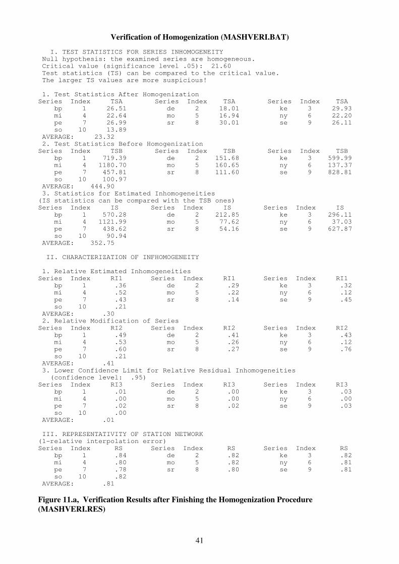
Verification of Homogenization (MASHVERI.BAT) I. TEST STATISTICS FOR SERIES INHOMOGENEITY Null hypothesis: the examined series are homogeneous. Critical value (significance level .05): 21.60 Test statistics (TS) can be compared to the critical value. The larger TS values are more suspicious! 1. Test Statistics After Homogenization Series Index TSA Series Index TSA Series Index TSA bp 1 26.51 de 2 18.01 ke 3 29.93 mi 4 22.64 mo 5 16.94 ny 6 22.20 pe 7 26.99 sr 8 30.01 se 9 26.11 so 10 13.89 AVERAGE: 23.32 2. Test Statistics Before Homogenization Series Index TSB Series Index TSB Series Index TSB bp 1 719.39 de 2 151.68 ke 3 599.99 mi 4 1180.70 mo 5 160.65 ny 6 137.37 pe 7 457.81 sr 8 111.60 se 9 828.81 so 10 100.97 AVERAGE: 444.90 3. Statistics for Estimated Inhomogeneities (IS statistics can be compared with the TSB ones) Series Index IS Series Index IS Series Index IS bp 1 570.28 de 2 212.85 ke 3 296.11 mi 4 1121.99 mo 5 77.62 ny 6 37.03 pe 7 438.62 sr 8 54.16 se 9 627.87 so 10 90.94 AVERAGE: 352.75 II. CHARACTERIZATION OF INFHOMOGENEITY 1. Relative Estimated Inhomogeneities Series Index RI1 Series Index RI1 Series Index RI1 bp 1 .36 de 2 .29 ke 3 .32 mi 4 .52 mo 5 .22 ny 6 .12 pe 7 .43 sr 8 .14 se 9 .45 so 10 .21 AVERAGE: .30 2. Relative Modification of Series Series Index RI2 Series Index RI2 Series Index RI2 bp 1 .49 de 2 .41 ke 3 .43 mi 4 .53 mo 5 .26 ny 6 .12 pe 7 .60 sr 8 .27 se 9 .76 so 10 .21 AVERAGE: .41 3. Lower Confidence Limit for Relative Residual Inhomogeneities (confidence level: .95) Series Index RI3 Series Index RI3 Series Index RI3 bp 1 .01 de 2 .00 ke 3 .03 mi 4 .00 mo 5 .00 ny 6 .00 pe 7 .02 sr 8 .02 se 9 .03 so 10 .00 AVERAGE: .01 III. REPRESENTATIVITY OF STATION NETWORK (1-relative interpolation error) Series Index RS Series Index RS Series Index RS bp 1 .84 de 2 .82 ke 3 .82 mi 4 .80 mo 5 .82 ny 6 .81 pe 7 .78 sr 8 .80 se 9 .81 so 10 .82 AVERAGE: .81

Figure 11.a, Verification Results after Finishing the Homogenization Procedure

(MASHVERI.RES)

42

EVALUATION OF META DATA IV. TEST STATISTICS Null hypothesis: the inhomogeneities can be explained by the Meta Data. Critical value (significance level .05): 21.60 Test statistics (TSM) can be compared to the critical value. The larger TSM values are more suspicious! Series Index TSM Series Index TSM Series Index TSM bp 1 53.09 de 2 41.63 ke 3 96.93 mi 4 1180.70 mo 5 88.35 ny 6 120.16 pe 7 228.76 sr 8 41.62 se 9 92.58 so 10 77.92 AVERAGE: 202.17 V. REPRESENTATIVITY OF META DATA (Relative part of estimated inhomogeneity can be explained by the Meta Data) Series Index RM Series Index RM Series Index RM bp 1 .55 de 2 1.00 ke 3 .33 mi 4 .04 mo 5 .20 ny 6 .05 pe 7 .49 sr 8 1.00 se 9 .52 so 10 .05 AVERAGE: .42

Figure 11.b, Verification Results for Meta Data after Finishing the Homogenization

Procedure (MASHVERI.RES)

43

VI. EXAMPLE FOR APPLICATION OF SAM SYSTEM Data Files (monthly series): m{j} ( j=1,....,12 )

Examined Series: Hungarian monthly mean temperature series (1901-1930).

Examined Stations: 1. Budapest (bp), 2. Debrecen (de), 3. Kecskemét (ke), 4. Miskolc (mi), 5. Mosonmagyaróvár (mo), 6. Nyíregyháza (ny), 7. Pécs (pe), 8. Sopron (sr), 9. Szeged (se), 10. Szombathely (so) Table of Reference System: HUNTEMP.REF TABLE OF REFERENCE SYSTEM (two rows belong to each examined series) row 1: index of candidate series(I3); number of reference series(I3) row 2: indexes of reference series(I3) 1 9 2 3 4 5 6 7 8 9 10 2 6 1 3 4 6 7 9 3 9 1 2 4 5 6 7 8 9 10 4 9 1 2 3 5 6 7 8 9 10 5 7 1 3 4 7 8 9 10 6 6 1 2 3 4 7 9 7 9 1 2 3 4 5 6 8 9 10 8 7 1 3 4 5 7 9 10 9 9 1 2 3 4 5 6 7 8 10 10 7 1 3 4 5 7 8 9

Table of Filambda Station Coordinates: HUNCOORD.PAR

index lambda(x) fi(y) 1 19.02499960 47.50833510 Budapest 2 21.60833360 47.49166490 Debrecen . . 9 20.09166720 46.25833510 Szeged 10 16.63333320 47.26666640 Szombathely

Table of META DATA: HUNMETA.DAT (for the given period) TABLE OF META DATA (one or two rows belong to each examined series) row 1: index of examined series(I3); number of meta data(I5) row 2: meta data(I5), if they exist 1 1 1909 2 0 3 0 4 1 1922 5 0 6 0 7 0 8 0 9 0 10 0

44

30 1020.53a12.00 7.44 .05 Model: additive Number of stations: 10 Length of series: 30 Significance level: .05 Critical value for break points: 20.53 Critical value for correction: 12.00 Critical value for outliers: 7.44 EXAMINED STATIONS AND INDEXES bp: 1 de: 2 ke: 3 mi: 4 mo: 5 ny: 6 pe: 7 sr: 8 se: 9 so:10 TABLE OF REFERENCE SYSTEM (two rows belong to each examined station) row 1: index of candidate station(I3); number of reference stations(I3) row 2: indexes of reference stations(I3) 1 9 2 3 4 5 6 7 8 9 10 2 6 1 3 4 6 7 9 3 9 1 2 4 5 6 7 8 9 10 4 9 1 2 3 5 6 7 8 9 10 5 7 1 3 4 7 8 9 10 6 6 1 2 3 4 7 9 7 9 1 2 3 4 5 6 8 9 10 8 7 1 3 4 5 7 9 10 9 9 1 2 3 4 5 6 7 8 10 10 7 1 3 4 5 7 8 9 File of Meta Data: MESHMETA.DAT Original monthly series: M{J}, (J=1,..,12) Original seasonal series: S{J}, (J=1,2,3,4) (winter,spring,summer,autumn) Original annual series: YEAR Homogenized monthly series: M{J}H, (J=1,..,12) Homogenized seasonal series: S{J}H, (J=1,2,3,4) (winter,spring,summer,autumn) Homogenized annual series: YEARH Inhomogeneity series for months: M{J}I, (J=1,..,12) Inhomogeneity series for seasons: S{J}I, (J=1,2,3,4) (winter,spring,summer,autumn) Inhomogeneity series for year: YEARI Break Points and Shifts for months: M{J}C, (J=1,..,12) Break Points and Shifts for seasons: S{J}C, (J=1,2,3,4) (winter,spring,summer,autumn) Break Points and Shifts for year: YEARC Taking the chosen monthly or seasonal series In: SAMIN.BAT Taking the chosen monthly or seasonal series Out: SAMOUT.BAT MONTHS with MISSING VALUES: 7 8

Figure 1. Output of Parametrization (SAMPAR.PAR)

45

1. Taking Month August In (SAMIN.BAT) TAKING SERIES IN SEASONAL INDEXES MONTHS: 1, 2, 3, 4, 5, 6, 7, 8, 9, 10, 11, 12 WINTER: 13 SPRING: 14 SUMMER: 15 AUTUMN: 16 YEAR: 17 MONTHS with MISSING VALUES: 7 8 MONTHS without FILLING : 7 8 Index?

8 (for example) EXAMINED STATIONS AND INDEXES bp: 1 de: 2 ke: 3 mi: 4 mo: 5 ny: 6 pe: 7 sr: 8 se: 9 so:10 Information, Parameters: SAMPAR.PAR, MASHPAR.PAR File of Meta Data: MASHMETA.DAT Original series (with missing values): MASHMISS.SER Original series (without missing values): MASHDAT.SER Homogenized series: MASHHOM.SER Inhomogeneity series: MASHINH.SER Break Points and Shifts: MASHCOR.RES Automatic filling of missing values: MASHMISS.BAT Help for selection of candidate series: MASHHELP.BAT Evaluation of Meta Data: METAHELP.BAT Automatic correction of outliers: MASHLIER.BAT GAME of MASH: MASHGAME.BAT Automatic version of GAME of MASH: MASHGAUT.BAT Comparing Test for seasonal series: SAMTESTC.BAT Selecting Test Procedure for seasonal series: SAMTESTS.BAT Non-automatic correction: MASHCOR.BAT Graphics: MASHDRAW.BAT MISSING VALUES! THE FIRST STEP: MASHMISS.BAT

Figure 2. Partial Output of Program SAMIN.BAT on the Screen

2.The Further Steps

Filling of missing values (MASHMISS.BAT); Correction of outliers (MASHLIER.BAT); Taking month AUGUST Out (SAMOUT.BAT).

Taking month JULY In (SAMIN.BAT); Filling of missing values (MASHMISS.BAT); Correction of outliers (MASHLIER.BAT); Taking month JULY Out (SAMOUT.BAT). Taking month JUNE In (SAMIN.BAT); Correction of outliers (MASHLIER.BAT); Taking month JUNE Out (SAMOUT.BAT).

46

3.The Next Steps: Examination of Season SUMMER

There is a possibility for examination of the seasonal series instead of the monthly series. The monthly inhomogeneities can be corrected by usage of the detected seasonal inhomogeneities, if the monthly inhomogeneities are identical within the given season.

3.1 Taking Season SUMMER In (SAMIN.BAT), Application of Program SAMTESTC.BAT HELP: TEST TABLE COMPARISON between June and Summer Null hypothesis: the monthly and the seasonal inhomogeneities are identical. Critical value (significance level .05): 20.53 Test statistics (TS) can be compared to the critical value. The larger TS values are more suspicious!

Station Index TS Station Index TS Station Index TS bp 1 10.20 de 2 11.14 ke 3 9.79 mi 4 18.65 mo 5 19.96 ny 6 15.74 pe 7 4.56 sr 8 20.84 se 9 15.90 so 10 9.78 HELP: TEST TABLE COMPARISON between July and Summer Null hypothesis: the monthly and the seasonal inhomogeneities are identical. Critical value (significance level .05): 20.53 Test statistics (TS) can be compared to the critical value. The larger TS values are more suspicious!

Station Index TS Station Index TS Station Index TS bp 1 15.87 de 2 24.45 ke 3 47.06 mi 4 12.33 mo 5 22.01 ny 6 8.07 pe 7 10.68 sr 8 11.75 se 9 7.75 so 10 12.32 HELP: TEST TABLE COMPARISON between August and Summer Null hypothesis: the monthly and the seasonal inhomogeneities are identical. Critical value (significance level .05): 20.53 Test statistics (TS) can be compared to the critical value. The larger TS values are more suspicious!

Station Index TS Station Index TS Station Index TS bp 1 20.19 de 2 8.62 ke 3 10.28 mi 4 15.02 mo 5 21.56 ny 6 8.36 pe 7 21.42 sr 8 4.99 se 9 25.89 so 10 19.83

Figure 3. Output of Test Program SAMTESTC.BAT (SAMTESTC.RES)

It can be seen that the null hypothesis can not be accepted for all the stations. The examination can be continued with a Test Procedure for excluding stations having different inhomogeneities between the seasonal series and the appropriate monthly series (SAMTESTS.BAT).

47

3.2 Application of Program SAMTESTS.BAT HELP: TEST TABLE FOR EXCLUDING STATIONS COMPARISON between June and Summer Null hypothesis: the monthly and the seasonal inhomogeneities are identical. Critical value (significance level .05): 20.53 Test statistics (TS) can be compared to the critical value. The larger TS values are more suspicious! Stations marked with asterisk(*) are not used for reference stations. Reference stations marked with asterisk(*) are excluded,i.e. null hypothesis is rejected.

Candidate station: ke Index: 3 Test Statistic: 16.03* Reference station: bp Index: 1 Test Statistic: 3.87 Reference station: de Index: 2 Test Statistic: 7.38 Reference station: mi Index: 4 Test Statistic: 18.65 Reference station: mo Index: 5 Test Statistic: 19.96* Reference station: ny Index: 6 Test Statistic: 15.74 Reference station: pe Index: 7 Test Statistic: 7.04 Reference station: sr Index: 8 Test Statistic: 18.63 Reference station: se Index: 9 Test Statistic: 15.90* Reference station: so Index: 10 Test Statistic: 4.67 COMPARISON between July and Summer Null hypothesis: the monthly and the seasonal inhomogeneities are identical. Critical value (significance level .05): 20.53 Test statistics (TS) can be compared to the critical value. The larger TS values are more suspicious! Stations marked with asterisk(*) are not used for reference stations. Reference stations marked with asterisk(*) are excluded,i.e. null hypothesis is rejected.

Candidate station: ke Index: 3 Test Statistic: 32.68* Reference station: bp Index: 1 Test Statistic: 10.71 Reference station: de Index: 2 Test Statistic: 16.43 Reference station: mi Index: 4 Test Statistic: 12.33 Reference station: mo Index: 5 Test Statistic: 22.01* Reference station: ny Index: 6 Test Statistic: 8.07 Reference station: pe Index: 7 Test Statistic: 5.15 Reference station: sr Index: 8 Test Statistic: 12.26 Reference station: se Index: 9 Test Statistic: 10.38* Reference station: so Index: 10 Test Statistic: 3.76 COMPARISON between August and Summer Null hypothesis: the monthly and the seasonal inhomogeneities are identical. Critical value (significance level .05): 20.53 Test statistics (TS) can be compared to the critical value. The larger TS values are more suspicious! Stations marked with asterisk(*) are not used for reference stations. Reference stations marked with asterisk(*) are excluded,i.e. null hypothesis is rejected.

Candidate station: ke Index: 3 Test Statistic: 10.28* Reference station: bp Index: 1 Test Statistic: 12.49 Reference station: de Index: 2 Test Statistic: 8.91 Reference station: mi Index: 4 Test Statistic: 15.02 Reference station: mo Index: 5 Test Statistic: 21.56* Reference station: ny Index: 6 Test Statistic: 8.36 Reference station: pe Index: 7 Test Statistic: 8.95 Reference station: sr Index: 8 Test Statistic: 15.59 Reference station: se Index: 9 Test Statistic: 25.89* Reference station: so Index: 10 Test Statistic: 9.42

Indexes of excluded stations: 3, 5, 9

Figure 4. Result Output of Test Program SAMTESTS.BAT (SAMTESTS.RES)

48

3.3 Homogenization of the SUMMER Series (MASHGAME.BAT, MASHGAUT.BAT etc.) ESTIMATED BREAK POINTS AND SHIFTS (Mark M: META DATA) bp: M1909: .26 de: No Break Points ke: 1927: .39/ 1928: -.39 mi: 1908: -3.74 mo: No Break Points ny: 1901: .93 pe: 1918: .52/ 1921: -1.18 sr: No Break Points se: 1918: -.76 so: 1917: .25

Figure 5. Detected SUMMER Inhomogeneities (MASHCOR.RES)

3.4 Evaluation of the Homogenization of SUMMER Series STAGE FIRST Null hypothesis: the examined series are homogeneous. Critical value (significance level .05): 20.53 Test statistics (TS) can be compared to the critical value. The larger TS values are more suspicious!

Series Index TS Series Index TS Series Index TS bp 1 87.15 de 2 22.40 ke 3 36.23 mi 4 1012.34 mo 5 27.64 ny 6 39.53 pe 7 82.45 sr 8 8.01 se 9 68.63 so 10 84.04 STAGE LAST Null hypothesis: the examined series are homogeneous. Critical value (significance level .05): 20.53 Test statistics (TS) can be compared to the critical value. The larger TS values are more suspicious!


Figure 6. Output of MASHHELP.BAT before and after Homogenization

(MASHHELP.RES)

49

STAGE FIRST Null hypothesis: the inhomogeneities can be explained by the Meta Data. Critical value (significance level .05): 20.53 Test statistics (TSM) can be compared to the critical value. The larger TSM values are more suspicious!

Series Index TSM Series Index TSM Series Index TSM bp 1 9.18 de 2 20.45 ke 3 38.11 mi 4 971.28 mo 5 17.86 ny 6 39.53 pe 7 82.45 sr 8 8.01 se 9 71.13 so 10 68.18 STAGE LAST Null hypothesis: the inhomogeneities can be explained by the Meta Data. Critical value (significance level .05): 20.53 Test statistics (TSM) can be compared to the critical value. The larger TSM values are more suspicious!

Series Index TSM Series Index TSM Series Index TSM bp 1 7.93 de 2 7.85 ke 3 17.27 mi 4 18.34 mo 5 17.22 ny 6 10.23 pe 7 22.70 sr 8 4.91 se 9 19.79 so 10 14.84

Figure 7. Output of METAHELP.BAT before and after Homogenization

(METAHELP.RES)

3.5 Taking Season SUMMER Out (SAMOUT.BAT) Homogenization of summer (June, July, August) monthly series on the basis of the detected summer inhomogeneities with exception of stations ke (index:3), mo (index:5), se (index:9), as a result of the Test Program SAMTESTS.BAT (see Figure 4.)

4. Evaluation of the Homogenization of Monthly Series

4.1 Taking month JUNE In (SAMIN.BAT); Application of MASHHELP.BAT STAGE FIRST Null hypothesis: the examined series are homogeneous. Critical value (significance level .05): 20.53 Test statistics (TS) can be compared to the critical value. The larger TS values are more suspicious!




(MASHHELP.RES)

50

4.2 Taking Month JULY In (SAMIN.BAT); Application of MASHHELP.BAT STAGE FIRST Null hypothesis: the examined series are homogeneous. Critical value (significance level .05): 20.53 Test statistics (TS) can be compared to the critical value. The larger TS values are more suspicious!




(MASHHELP.RES)

4.3 Taking Month AUGUST In (SAMIN.BAT); Application of MASHHELP.BAT STAGE FIRST Null hypothesis: the examined series are homogeneous. Critical value (significance level .05): 20.53 Test statistics (TS) can be compared to the critical value. The larger TS values are more suspicious!




(MASHHELP.RES)

51

5. Verification of Homogenization for SUMMER series (MASHVERI.BAT) I. TEST STATISTICS FOR SERIES INHOMOGENEITY Null hypothesis: the examined series are homogeneous. Critical value (significance level .05): 20.53 Test statistics (TS) can be compared to the critical value. The larger TS values are more suspicious! 1. Test Statistics After Homogenization Series Index TSA Series Index TSA Series Index TSA bp 1 10.46 de 2 7.49 ke 3 39.51 mi 4 36.10 mo 5 19.10 ny 6 10.23 pe 7 40.89 sr 8 4.91 se 9 107.80 so 10 12.21 AVERAGE: 28.87 2. Test Statistics Before Homogenization Series Index TSB Series Index TSB Series Index TSB bp 1 97.39 de 2 17.04 ke 3 39.72 mi 4 1012.34 mo 5 27.64 ny 6 39.53 pe 7 82.45 sr 8 8.01 se 9 68.75 so 10 84.04 AVERAGE: 147.69 3. Statistics for Estimated Inhomogeneities (IS statistics can be compared with the TSB ones) Series Index IS Series Index IS Series Index IS bp 1 19.29 de 2 .00 ke 3 3.27 mi 4 889.88 mo 5 .00 ny 6 17.29 pe 7 42.41 sr 8 .00 se 9 .00 so 10 9.29 AVERAGE: 98.14 II. CHARACTERIZATION OF INFHOMOGENEITY 1. Relative Estimated Inhomogeneities Series Index RI1 Series Index RI1 Series Index RI1 bp 1 .13 de 2 .00 ke 3 .08 mi 4 .98 mo 5 .00 ny 6 .18 pe 7 .31 sr 8 .00 se 9 .00 so 10 .15 AVERAGE: .18 2. Relative Modification of Series Series Index RI2 Series Index RI2 Series Index RI2 bp 1 .15 de 2 .00 ke 3 .08 mi 4 1.14 mo 5 .00 ny 6 .18 pe 7 .54 sr 8 .00 se 9 .00 so 10 .22 AVERAGE: .23 3. Lower Confidence Limit for Relative Residual Inhomogeneities (confidence level: .95) Series Index RI3 Series Index RI3 Series Index RI3 bp 1 .00 de 2 .00 ke 3 .08 mi 4 .06 mo 5 .00 ny 6 .00 pe 7 .09 sr 8 .00 se 9 .24 so 10 .00 AVERAGE: .05 III. REPRESENTATIVITY OF STATION NETWORK (1-relative interpolation error) Series Index RS Series Index RS Series Index RS bp 1 .84 de 2 .79 ke 3 .70 mi 4 .65 mo 5 .79 ny 6 .74 pe 7 .73 sr 8 .64 se 9 .80 so 10 .75 AVERAGE: .74

Figure 11.a, Verification Results at the actual stage of Homogenization

(MASHVERI.RES)

52

EVALUATION OF META DATA IV. TEST STATISTICS Null hypothesis: the inhomogeneities can be explained by the Meta Data. Critical value (significance level .05): 20.53 Test statistics (TSM) can be compared to the critical value. The larger TSM values are more suspicious! Series Index TSM Series Index TSM Series Index TSM bp 1 10.42 de 2 16.54 ke 3 39.72 mi 4 971.28 mo 5 17.86 ny 6 39.53 pe 7 82.45 sr 8 8.01 se 9 71.23 so 10 68.18 AVERAGE: 132.52 V. REPRESENTATIVITY OF META DATA (Relative part of estimated inhomogeneity can be explained by the Meta Data) Series Index RM Series Index RM Series Index RM bp 1 1.00 de 2 1.00 ke 3 .00 mi 4 .07 mo 5 1.00 ny 6 .00 pe 7 .00 sr 8 1.00 se 9 1.00 so 10 .00 AVERAGE: .51

Figure 11.b, Verification Results for Meta Data at the actual stage of Homogenization

(MASHVERI.RES)

53

VII. HOMOGENIZATION OF DAILY DATA

MATHEMATICAL BASIS (draft version)

Only the additive model is presented that is appropriate for temperature, pressure etc. elements. Relation of daily and monthly homogenization

Alternative possibilities – To use the detected monthly inhomogeneities directly for daily data homogenization – Direct methods for daily data homogenization Problems – The direct use of the detected monthly inhomogeneities is probably not sufficient. – Direct methods for daily data homogenization is probably not enough efficient thinking of the larger variability (less signal to noise ratio). The Question How can we use the valuable information of detected monthly inhomogeneities for daily data homogenization? Additive model for daily values (e.g. temperature)

( ) ( ) ( ) ( ) ( )dmydmyIHdmdmydmyXstststst ,,,,,,,,, 0 εµµ +++=

µ : climate change signal, 0µ : spatial expected value,

IH : inhomogeneity , ε : normal noise

st : station, m : month, y : year, d : day

Additive model for monthly means

( ) ( ) ( ) ( )yyIHyyX st

m

st

m

st

mm

st

m εµµ +++= 0

( ) ( )myIHyIH stst

m ,= : inhomogeneity (break points and shifts)

We have: estimated monthly inhomogeneities: ( )yHIst

mˆ

Valuable information! : ( ) ( )yIHmyIH st

m

st =,

But maybe a problem of direct use: the smoothness Question:

Smooth estimation ( )dmyHI st ,,ˆ for daily inhomogeneities

by using the estimated monthly inhomogeneities ( )yHIst

mˆ ?

Possible condition for daily estimation ( )dmyHI st ,,ˆ :

Smoothness and condition for mean: ( ) ( )yHImyHI st

m

st ˆ,ˆ =

Maybe a problem: too strong inhomogeneities can be obtained.

54

Other train of thought

Not to forget: the monthly values ( )yHIst

mˆ are only estimations,

stochastic variables. To know the real ( )yIH st

m is impossible.

Consequently the monthly estimations ( )yHIst

mˆ may be modified.

But the modification must be controlled.

The Essence of Procedure

i, Smooth estimation for daily inhomogeneities with

a not too strong condition e.g.: ( ) ( )yHIdmyHId st

m

st ˆ,,ˆ: 00 =∃

ii, Test of hypothesis to control the new monthly estimations:

( ) ( )myHIyHI stst

m ,ˆ:~

=

The MASH Procedure for Daily Data

1. Monthly means ( )yX st

m from daily data ( )dmyXst ,, .

2. MASH homogenization procedure for monthly series ( )yX st

m ,

estimation of monthly inhomogeneities: ( )yHIst

mˆ

3. On the basis of estimated monthly inhomogeneities ( )yHIst

mˆ ,

smooth estimation for daily inhomogeneities: ( )dmyHI st ,,ˆ .

4. Homogenization of daily data:

( ) ( ) ( )dmyHIdmyXdmyX ststst ,,ˆ,,,,~

−= .

5. Qulity Control for homogenized daily data ( )dmyX st ,,~

.

6. Missing daily data complementing.

7. Monthly means ( )yXst

m

~ from homogenized, controlled, complemented

daily data ( )dmyX st ,,~

.

8. Test of homogeneity for the new monthly series ( )yXst

m

~ by MASH.

Repeating steps 2-8 with ( )yXst

m

~, ( )dmyX st ,,

~ if it is necessary.

Interpolation technique for QC and Data Complementing

Daily data for a given month:

( ) ( ) ( )( )tDtENtX jjj ,∈ ( )30,...,1;station,..,1 == tMj

Candidate data: ( )tX j Reference data: ( ) ( )jitX i ≠

55

Interpolation: ( ) ( ) ( ) ( )∑≠

+=ji

ijijj tXtwtwtX 0ˆ where ( ) 1=∑

≠ ji

ji tw .

RMS Error and Representativity: ( )tRMSE j , ( )( )

( )tD

tRMSEtREP

j

j

j −= 1

The Optimum Interpolation Parameters ( ) ( ) ( )30,..,1;,0 =≠ tjitwtw opt

ji

opt

j

minimizing ( )tRMSE j , are uniquely determined by the expectations,

st. deviations and the correlations. Problem: Estimation of daily statistical parameters. Assumptions:

i, ( ) ( ) jiij etEtE =− , ( ) ( ) jiij dtDtD = , ( )30,..,1; =≠ tji

ii, ( ) ( )( ) T

tt

S

jjjj rrtXtX212121 21 ,corr ⋅= ( )30,..,1,;,...1, 2121 == ttMjj

S

jjr21: correlation structure in space, T

ttr 21: correlation structure in time

⇔ Partial corr.: ( ) ( ) ( )( ) =21 2121,corr tXtX jjtX j ( ) ( ) ( )( ) 0,corr 21 2112

=tXtX jjtX j

Statement: If the assumptions i, ii, are fulfilled then

( ) ( ) ( ) ( )30,..,1,,00 =≡≡≡ tREPtREPwtwwtwopt

j

opt

j

opt

ji

opt

ji

opt

j

opt

j ,

where opt

j

opt

ji

opt

j REPww ,,0 are the optimal parameters of monthly

interpolation: ( ) ∑≠

+=ji

ijijj XwwtX 0ˆ where 1=∑

≠ ji

jiw .

Consequence

The monthly statistical parameters can be used for daily interpolation.

i, Data Complementing: ( ) ( )∑≠

+=ji

i

opt

ji

opt

jj tXwwtX 0ˆ

ii, Quality Cotrol can be based on the standardized error:

( )( ) ( )

( )( )opt

jj

jj

jREPtD

tXtXtZ

−

−=

1

ˆ ( )1,0N∈

where opt

j

opt

ji

opt

j REPww ,,0 are the optimal parameters of monthly

interpolation, and ( )tD j is the daily standard deviation.

56

Test of Hypothesis of the standardized error series ( )tZ ( )nt ,..,1=

If the data have good quality then ( ) ( )1,0NtZ ∈ ( )nt ,..,1= .

But Problem: ( )

< ztZt

maxP depends on the autocorrelation.

Statement:

i, If ( )tZ ( )nt ,..,1= is a Markov process, furthemore

ii, and ( ) ( )( ) ( )( )ztZztZztZ <≥<−< P1P

( )nt ,..,2= ,

then ( ) ( )( )∏=

<≥

<n

t

ztZztZt 1

PmaxP .

Example:

If ( )tZ ( )nt ,..,1= is a normal AR(1) process then i, ii, are fulfilled.

Decision according to test of hypothesis

We have wrong data:

If ( ) pztZ > where critical value pz is defined by

the significance level p (e.g.: p=0.01) as,

( ) ≥

< pztZt

maxP ( )( ) pzn

p −=−Φ 112 ,

( )zΦ : standard normal distribution function.

Multiple QC for daily data

More standardized error series are examined without common

reference series to separate the wrong data for the candidate station.

Correction of the wrong data is based on confidence intervals.

57

THE STRUCTURE OF MASHDAILY PROGRAM SYSTEM

Main Directory MASHv3.02:

Directory MASHDAILY:

- Subdirectory MASHDAMO

- MASHDAMO.BAT

- Subdirectory MASHFORMAT

- Subdirectory MASHDAMOSUB (do not use it including "subroutines")

- Subdirectory MASHDAILY:

- Subdirectory MASHDPAR - Parametrization program: MASHDPAR.BAT - Main Program: MASHD.BAT

- Subdirectory MASHDSUB (do not use it including "subroutines")

Directory MASHMONTHLY (See Page 21)

MASHDAILY IN PRACTICE

I. Monthly Data from Daily Data in Subdirectory MASHDAILY\ MASHDAMO

MASHDAMO.BAT (see page 58)

II. Homogenization of Monthly Series in Directory MASHMONTHLY\SAM

MASH homogenization procedure for monthly series, estimation of monthly inhomogeneities. Input Files from MASHDAMO\MASHFORMAT: M{j} (j=1,....,12), FILASTAT.PAR (see p. 58; Copy batch File in Subdirectory MASHFORMAT: COPYSAMPAR.BAT) III. Homogenization of Daily Data in Subdirectory MASHDAILY\ MASHDAILY

1. Parametrization in Subdirectory MASHDAILY\ MASHDAILY\MASHDPAR:

MASHDPAR.BAT (see pages 58-59) 2. Homogenization of Daily Data, Qulity Control for Homogenized Daily Data, Missing

Daily Data Complementing in Subdirectory MASHDAILY\ MASHDAILY:

MASHD.BAT (see pages 59-60)

58

THE MAIN PROGRAM and I/O FILES in Subdirectory MASHDAMO

EXECUTIVE FILE: MASHDAMO.BAT

INPUT:

Original Daily Data: DAILY.DAT Maximal number of stations: 500 Maximal number of years: 200 Format of Data File: row 1: names of stations (obligatory!), Format: (2x,character*6)? column 1: date of year (I4) column 2: month (I2) column 3: day (I2) column i+3: series i. Data Format: F8.2 Mark of Missing Values: 9999.99

File of Filambda Station Coordinates: FILASTAT.PAR (see page 61)

Model: additive or multiplicative

RESULT OUTPUT FILES in MASHDAMO\MASHFORMAT:

(Input Files of MASHMONTHLY\SAM) Files of Monthly Series: M{J} (J=1,..,12) File of Filambda Station Coordinates: FILASTAT.PAR

RESULT OUTPUT FILES in MASHDAILY\MASHDPAR: Original Daily Data: DAILY.DAT Files of Monthly Series: M{J} (J=1,..,12) File of Filambda Station Coordinates: FILASTAT.PAR Parameter File: MASHDPAR.PAR

THE MAIN PROGRAM and I/O FILES of Subdirectory

MASHDAILY\ MASHDAILY\MASHDPAR

EXECUTIVE BATCH FILE: MASHDPAR.BAT

THE STEPS OF MASHDPAR.BAT: MASHDTRAN.EXE & MASHDTOP.EXE& MASHDTEXT.EXE

INPUT DATA FILES:

Result Files from MASHMONTHLY\SAM\SAMEND: Homogenized Monthly Series M{j}h ( j=1,....,12 )

Monthly Inhomogeneities M{j}i ( j=1,....,12 )

(Copy batch File in Subdirectory SAMEND: COPYMASHDPAR)

INPUT DATA FILES DAILY.DAT, M{J} (J=1,..,12), MASHDPAR.PAR, FILASTAT.PAR are written in by MASHDAMO.BAT

59

OUTPUT FILES written in Directory MASHDAILY\MASHDAILY:

MASHDPAR.PAR, FILASTAT.PAR, REFERENCE.PAR, DAILY.DAT, M{j} (j=1,....,12), M{j}h (j=1,....,12), M{j}i (j=1,....,12) Work and Parameter Files: DMP{j}.PAR ( j=1,....,6 ), M{j}h.tr (j=1,....,12)

THE MAIN PROGRAM and I/O FILES of Subdirectory

MASHDAILY\ MASHDAILY

EXECUTIVE BATCH FILE: MASHD.BAT

INPUT DATA FILES are written in by MASHDPAR.BAT RESULT OUTPUT FILES:

Homogenized, Controlled and Complemented daily Data: DAILYHOMQC.DAT

Homogenized and Complemented daily Data (without QC): DAILYHOM.DAT

Daily Inhomogeneities: DAILYINHOM.DAT

Result of Quality Control: ERROR.RES

THE STEPS OF MASHD.BAT:

1. STAT1.EXE: Input: MASHDPAR.PAR, M{j}h ( j=1,....,12 ), FILASTAT.PAR Output: STAT1{j}.PAR ( j=1,....,12 ) 2. DMINHOM1.EXE: Input: MASHDPAR.PAR, M{j} ( j=1,....,12 ), M{j}i ( j=1,....,12 ) Output: DMSTAT.RES, DM{j}i.PAR ( j=1,....,12 ) 3. DMINHOM2.EXE: Input: MASHDPAR.PAR, M{j} ( j=1,....,12 ), M{j}i ( j=1,....,12 ) Output: DM{j}i ( j=1,....,12 ) 4. DMINHOM3.EXE: Input: MASHDPAR.PAR, DM{j}i ( j=1,....,12 ) Output: DM{j}i ( j=1,....,12 ) (Daily inhomogeneities in 12 files) 5. DMDATA.EXE: Input: MASHDPAR.PAR, DAILY.DAT Output: DM{j} ( j=1,....,12 ) (Original daily data in 12 files)

60

6. DMINHCORR.EXE: Input: MASHDPAR.PAR, DM{j}i.PAR ( j=1,....,12 ), DM{j}i ( j=1,....,12 ), DM{j} ( j=1,....,12 ) Output: DM{j}h ( j=1,....,12 ) (Homogenized daily data in 12 files), DM{j}d ( j=1,....,12 ) (Daily st. deviations in 12 files) 7. QC.EXE Input: MASHDPAR.PAR, REFERENCE.PAR, STAT1{j}.PAR ( j=1,....,12 ), DM{j}i ( j=1,....,12 ), DM{j}h ( j=1,....,12 ), DM{j}d ( j=1,....,12 ), DM{j} ( j=1,....,12 ), M{j}i ( j=1,....,12 ) Output: DM{j}hc ( j=1,....,12 ) (Homogenized, controlled daily data in 12 files) ERROR.RES

Work and Parameter Files: QC1.PAR, QC2.PAR, ERR{j} ( j=1,....,12 ), ERROR.PAR 8. MISSING.EXE: Input: MASHDPAR.PAR, FILASTAT.PAR, DM{j}hc ( j=1,....,12 ), STAT1{j}.PAR (i=1,..12) Output: DM{j}hcm ( j=1,....,12 ) (Homog., controlled, complemented daily data in 12 files) Work and Parameter Files: MISSING1.PAR, MISSING2.PAR 9. DAILYEND.EXE: Input: MASHDPAR.PAR, DM{j}hcm ( j=1,....,12 ), DM{j}i ( j=1,....,12 ) Output: DAILYHOMQC.DAT, DAILYHOM.DAT, DAILYINHOM.DAT

61

EXAMPLE FOR APPLICATION OF MASHDAILY SYSTEM Examined Data: DAILY.DAT

Daily temperature series (1901-1930), 10 Stations in Hungary.

Temperature element: (max+min)/2

Model: additive File of Filambda Station Coordinates: FILASTAT.PAR

index lambda(x) fi(y) 1 18.65308760 47.18486400 2 20.62684630 46.57159040 3 17.09815790 47.05921170 4 20.14969640 47.21730420 5 17.39957430 47.90058140 6 20.80181500 46.85120390 7 16.83021930 47.91734310 8 19.18956180 45.94506840 9 16.73989490 47.59620290 10 19.86032100 46.45614240

Estimated Monthly Inhomogeneities for a year

-3

-2,5

-2

-1,5

-1

-0,5

0

0,5

1

1,5

1 31 61 91 121 151 181 211 241 271 301 331 361

Smoothed Monthly Inhomogeneities (Estimated Daily Inhomogeneities)

-3

-2,5

-2

-1,5

-1

-0,5

0

0,5

1

1,5

1 31 61 91 121 151 181 211 241 271 301 331 361

Figure 1. Example for smoothing of Monthly Ihomogeneities

62

Detected errors in September 1903 at Station 10 (ERROR.RES)

st1 st2 st3 st4 st5 st6 st7 st8 st9 st10 1903 9 1 0.0 0.0 0.0 0.0 0.0 0.0 0.0 0.0 0.0 -3.4 1903 9 2 0.0 0.0 0.0 0.0 0.0 0.0 0.0 0.0 0.0 -2.2 1903 9 3 0.0 0.0 0.0 0.0 0.0 0.0 0.0 0.0 0.0 -3.1 1903 9 4 0.0 0.0 0.0 0.0 0.0 0.0 0.0 0.0 0.0 -5.0 1903 9 5 0.0 0.0 0.0 0.0 0.0 0.0 0.0 0.0 0.0 -2.6 1903 9 6 0.0 0.0 0.0 0.0 0.0 0.0 0.0 0.0 0.0 -2.7 1903 9 7 0.0 0.0 0.0 0.0 0.0 0.0 0.0 0.0 0.0 -4.9 1903 9 8 0.0 0.0 0.0 0.0 0.0 0.0 0.0 0.0 0.0 -2.9 1903 910 0.0 0.0 0.0 0.0 0.0 0.0 0.0 0.0 0.0 -1.8 1903 911 0.0 0.0 0.0 0.0 0.0 0.0 0.0 0.0 0.0 -5.5

Original Data

1903 9 1 20.5 17.1 20.0 17.5 21.0 18.1 18.7 19.5 19.3 12.3 1903 9 2 19.8 17.9 20.8 15.5 21.5 14.9 18.4 19.3 20.2 13.2 1903 9 3 19.1 17.3 20.8 15.5 21.3 15.8 18.5 17.2 17.5 11.3 1903 9 4 19.7 17.5 19.8 15.3 19.0 15.8 18.8 19.2 17.2 10.4 1903 9 5 20.3 17.8 20.5 16.0 21.0 17.4 19.3 20.4 17.8 13.2 1903 9 6 20.9 18.7 21.3 17.3 20.0 18.6 19.9 21.4 18.8 13.8 1903 9 7 22.9 21.5 22.5 17.8 22.0 19.5 18.9 23.6 19.0 13.9 1903 9 8 22.5 20.9 25.0 19.0 23.0 19.8 19.1 23.5 19.5 15.5 1903 910 17.7 18.4 17.0 13.8 13.6 19.0 14.3 18.9 13.7 12.7 1903 911 16.5 13.7 18.3 11.8 14.5 13.5 13.1 18.8 14.1 6.2

Longterm means in September

16.7 15.9 16.2 14.9 15.9 15.5 14.6 17.0 14.7 16.6

Figure 2. Part Results of Quality Control

TEST STATISTICS for ANNUAL SERIES (OUTPUT of MASH)

Critical value (significance level 0.05): 20.53

1. Test Statistics Before Monthly Homogenization

Station TSBM Station TSBM Station TSBM

4 317.85 6 241.41 2 155.04

9 127.66 7 91.66 10 68.36

1 62.55 8 61.84 5 42.06

3 15.82 AVERAGE: 118.42

2. Test Statistics After Monthly Homogenization

Station TSAM Station TSAM Station TSAM

7 28.64 5 25.11 9 22.73

4 18.52 1 18.12 8 15.26

6 14.96 2 14.82 10 12.41

3 10.26 AVERAGE: 18.08

3. Test Statistics After Monthly&Daily Homogenization

Station TSAMD Station TSAMD Station TSAMD

7 28.89 5 25.40 2 25.06

9 21.98 1 17.60 4 16.52

8 15.23 6 14.66 3 9.69

10 9.00 AVERAGE: 18.40

Figure 3. Verification Results for the Annual Series (MASHVERI.RES)

63

AVERAGED TEST STATISTICS FOR MONTHLY SERIES (10 Stations)

Average of Test Statistics Before Monthly Homogenization: TSBM

Average of Test Statistics After Monthly Homogenization: TSAM

Average of Test Statistics After Monthly&Daily Homogenization: TSAMD

MONTH TSBM TSAM TSAMD

1 28.5 12.0 12.1 2 21.1 16.6 17.0 3 41.2 24.0 22.4 4 73.7 17.5 17.8 5 82.1 15.7 13.4 6 100.7 14.7 12.5 7 84.5 16.1 14.2 8 61.7 16.0 14.3 9 131.4 12.9 13.1 10 56.3 14.6 16.0 11 38.9 10.4 11.2 12 34.5 18.7 20.4 SP 90.6 19.9 20.2 SU 92.6 18.7 17.2 AU 101.3 17.1 19.6 WI 32.1 18.3 16.6 Y 118.4 18.1 18.4

Critical value (significance level 0.05): 20.53

Test statistics (TS) can be compared to the critical value.

Figure 4. Average of Verification Results for the Monthly Series

64

ANNEX: SOME NEW DEVELOPMENTS FOR AUTOMATION

(‘User friendly’ procedures) 1. In Directory MASHMONTHLY\SAM\MASH

1.1. Automatic, iteration application of MASHGAME.BAT

(Iteration Examination of all the station series)

Directory: MASHMONTHLY\SAM\MASH\MASHAUTO

Batch Files:

i, MAUTOPAR.BAT: Parametrization Input: Number of Iteration Steps

ii, MASHAUTO.BAT: Examination, homogenization 2. In Directory MASHMONTHLY\SAM

2.1. Automatic, iteration application of MASHGAME.BAT

(Iteration Examination of all the station series)

Directory: MASHMONTHLY\SAM\SAMAUTO

Batch Files:

i, SAUTOPAR.BAT: Parametrization Input: Number of Iteration Steps

ii, SAMAUTO.BAT: Examination, homogenization 2.2. Data Complementing for all the 12 Months together

(Automatic version of MASHMISS.BAT)

Directory: MASHMONTHLY\SAM\SAMMISS

Batch File: SAMMISS.BAT 2.3. Verification Procedure for all Monthly, Seasonal and Annual Series together

(Automatic version of MASHVERI.BAT)

Directory: MASHMONTHLY\SAM\SAMVERI

Batch File: SAMVERI.BAT

Output Files in Directory SAM: V{j}. (j=1,….,17)

References Szentimrey, T., 1994: "Statistical problems connected with the homogenization of climatic time series", Proceedings of the European Workshop on Climate Variations, Kirkkonummi, Finland, Publications of the Academy of Finland, 3/94, pp. 330-339. Szentimrey, T., 1995: "Statistical methods for detection of inhomogeneities", Proceedings of the Regional Workshop on Climate Variability and Climate Change Vulnerability and Adaptation, Prague, pp. 293-298. Szentimrey, T., 1995: "General problems of the estimation of inhomogeneities, optimal weighting of the

reference stations", Proceedings of the 6h International Meeting on Statistical Climatology, Galway, Ireland, pp. 629-631. Szentimrey, T., 1996: "Some statistical problems of homogenization: break points detection, weighting of

reference series", Proceedings of the 13th

Conference on Probability and Statistics in the Atmospheric Sciences, San Francisco, California, pp. 365-368. Szentimrey, T., 1997: "Statistical procedure for joint homogenization of climatic time series", Proceedings of the Seminar for Homogenization of Surface Climatological Data, Budapest, Hungary, pp. 47-62. Peterson, T.C., Easterling, D.R., Karl, T.R., Groisman, P., Nicholls, N., Plummer, N., Torok, S., Auer, I., Boehm, R., Gullett, D., Vincent, L., Heino, R., Tuomenvirta, H., Mestre, O., Szentimrey, T., Salinger, J., Forland, E.J., Hanssen-Bauer, I., Alexanderson, H., Jones, P. and Parker D., 1998: “Homogeneity adjustments of in situ atmospheric climata data: a review”, International Journal of Climatology, 18: 1493-1517 Szentimrey, T., 1998: ”MASHv1.03”, Guide for Software Package, Hungarian Meteorological Service, Budapest, Hungary, p. 25. Auer, I., Böhm, R., 1998: “Endbericht des Projects ALOCLIM, Teil I-II”, Zentralanstalt für Meteorologie und Geodynamik, Wien.

Szentimrey, T., 1999: ”Multiple Analysis of Series for Homogenization (MASH)”, Proceedings of the Second Seminar for Homogenization of Surface Climatological Data, Budapest, Hungary; WMO, WCDMP-No. 41, pp. 27-46. Szentimrey, T., 2000: „Multiple Analysis of Series for Homogenization (MASH). Seasonal application of MASH (SAM), Automatic using of Meta Data”, Proceedings of the Third Seminar for Homogenization of Surface Climatological Data, Budapest, Hungary, Home page:http://omsz.met.hu/ismeretterjesztes/rendezvenyek/rendezveny_hu.html Auer, I., Böhm, R,. Schöner, W., 2001: “Austrian Long-Term Climate (ALOCLIM) 1767-2000 , Multiple instrumental climate time series from Central Europe”, Österreichische Beiträge zu Meteorologie und Geophysik, Heft 25, Central Institute for Meteorology and Geodynamics, Vienna. Szentimrey, T., 2002: “Statistical problems connected with the spatial interpolation of climatic time series.”, Home page:http://www.knmi.nl/samenw/cost719/documents/Szentimrey.pdf Szentimrey, T., 2003: „Homogenization software MASHv2.03”, Home page:http://www.wmo.ch/web/wcp/clips2001/html/MASH_software.htm Szentimrey, T., 2004: „Something like an Introduction”, Proceedings of the Fourth Seminar for Homogenization and Quality Control in Climatological Databases, Budapest, Hungary; WMO, WCDMP-No. 56, pp. 5-16. Szentimrey, T., 2004: „Multiple Analysis of Series for Homogenization (MASH); Verification procedure for homogenized time series”, Proceedings of the Fourth Seminar for Homogenization and Quality Control in Climatological Databases, Budapest, Hungary; WMO, WCDMP-No. 56, pp. 193-201.

Szentimrey, T., 2006: „An overview on the main methodological questions of homogenization”, Fifth Seminar for Homogenization and Quality Control in Climatological Databases, Budapest, Hungary. Szentimrey, T. 2006: „Development of MASH homogenization procedure for daily data”, Fifth Seminar for Homogenization and Quality Control in Climatological Databases, Budapest, Hungary. Szentimrey, T., Bihari, Z., 2007: „Mathematical background of the spatial interpolation methods and the software MISH (Meteorological Interpolation based on Surface Homogenized Data Basis)”, Proceedings from the Conference on Spatial Interpolation in Climatology and Meteorology, Budapest, Hungary, 2004, COST Action 719, COST Office, 2007, pp. 17-27 Szentimrey, T., 2007: „Manual of interpolation software MISHv1.02”, Hungarian Meteorological Service, p. 32 Here are some APN (Asia-Pacific Network) web sites connected with the MASH method: „Software Used by the APN Network for Climate Extremes” http://www.bom.gov.au/bmrc/csr/apn/software.html „A Guide to Programs for Calculating Indices of Extremes” http://www.bom.gov.au/bmrc/csr/apn/papers/apn_manual.pdf

multiple analysis of series for homogenization ( m a s h ... · preface of version mashv3.02 the...

Documents