Multilinear Least Square, Eigenvalue, and

Singular Value Problems

Lek-Heng Lim

Linear Algebra and Optimization Seminar

October 11, 2006

Thanks: Sou-Cheng Choi, Vin de Silva, Gene Golub, Morten

Mørup, Liqun Qi, Michael Saunders, Berkant Savas

[aij

]l×m

[bjk

]m×n

=[∑m

j=1aijbjk

]l×n

2

Tensors

A set of multiply indexed real numbers A = JaijkKl,m,ni,j,k=1 ∈ Rl×m×n

on which the following algebraic operations are defined:

1. Addition/Scalar Multiplication: for JbijkK ∈ Rl×m×n, λ ∈ R,

JaijkK+JbijkK := Jaijk+bijkK and λJaijkK := JλaijkK ∈ Rl×m×n

2. Multilinear Matrix Multiplication: for matrices L = [λi′i] ∈Rp×l, M = [µj′j] ∈ Rq×m, N = [νk′k] ∈ Rr×n,

(L, M, N) ·A := Jci′j′k′K ∈ Rp×q×r

where

ci′j′k′ :=l∑

i=1

m∑j=1

n∑k=1

λi′iµj′jνk′kaijk.

May think of A as a 3-dimensional array of numbers. (L, M, N)·Aas multiplication on ‘3 sides’ by matrices L, M, N .

3

Outer product rank

u ∈ Rl, v ∈ Rm, w ∈ Rn, outer product defined by

u⊗ v ⊗w = JuivjwkKl,m,ni,j,k=1.

A tensor A ∈ Rl×m×n is said to be decomposable if it can be

written in the form

A = u⊗ v ⊗w.

A ∈ Rl×m×n, outer product rank is

rank⊗(A) = min{r | A =∑r

i=1ui ⊗ vi ⊗wi}.

4

Tensor rank is difficult

Mystical Power of Twoness (Eugene L. Lawler). 2-SAT is

easy, 3-SAT is hard; 2-dimensional matching is easy, 3-dimensional

matching is hard; etc.

Matrix rank is easy, tensor rank is hard:

Theorem (Hastad). Computing rank⊗(A) for A ∈ Rl×m×n is an

NP-hard problem.

Tensor rank depends on base field:

Theorem (Bergman). For A ∈ Rl×m×n ⊂ Cl×m×n, rank⊗(A) is

base field dependent.

5

Best rank-r approximation of tensors

Given A ∈ Rl×m×n, solve

argminrank⊗(B)≤r‖A−B‖F .

No solution for all orders > 2, all norms, and many ranks:

Theorem 1 (de Silva, L). Let k ≥ 3 and d1, . . . , dk ≥ 2. For any

s such that 2 ≤ s ≤ min{d1, . . . , dk} − 1, there exist A ∈ Rd1×···×dk

with rank⊗(A) = s such that A has no best rank-r approximation

for some r < s. The result is independent of the choice of norms.

Tensor rank can jump over an arbitrarily large gap:

Theorem 2 (de Silva, L). Let k ≥ 3. Given any s ∈ N, there

exists a sequence of order-k tensor An such that rank⊗(An) ≤ r

and limn→∞An = A with rank⊗(A) = r + s.6

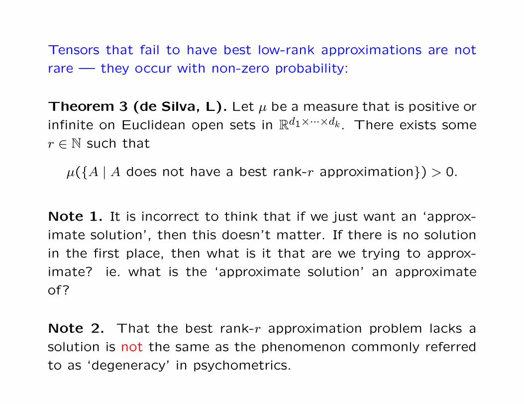
Tensors that fail to have best low-rank approximations are not

rare — they occur with non-zero probability:

Theorem 3 (de Silva, L). Let µ be a measure that is positive or

infinite on Euclidean open sets in Rd1×···×dk. There exists some

r ∈ N such that

µ({A | A does not have a best rank-r approximation}) > 0.

Note 1. It is incorrect to think that if we just want an ‘approx-

imate solution’, then this doesn’t matter. If there is no solution

in the first place, then what is it that are we trying to approx-

imate? ie. what is the ‘approximate solution’ an approximate

of?

Note 2. That the best rank-r approximation problem lacks a

solution is not the same as the phenomenon commonly referred

to as ‘degeneracy’ in psychometrics.

Message

Best rank-r approximation problem for tensors is difficult.

Let’s study something else.

7

Symmetric tensors

A = Jai1···ikK ∈ Rd1×···×dk. For a permutation σ ∈ Sk, σ-transpose

of A is

Aσ = Jaiσ(1)···iσ(k)K ∈ Rdσ(1)×···×dσ(k).

Order-k generalization of ‘taking transpose’.

For matrices (order-2), only one way to take transpose (ie. swap-

ping row and column indices) since S2 has only one non-trivial

element. For an order-k tensor, there are k!− 1 different ‘trans-

poses’ — one for each non-trivial element of Sk.

An order-k tensor A = Jai1···ikK ∈ Rn×···×n is called symmetric if

A = Aσ for all σ ∈ Sk, ie.

aiσ(1)···iσ(k)= ai1···ik.

8

Rayleigh-Ritz approach to eigenpairs

A ∈ Rn×n symmetric. Its eigenvalues and eigenvectors are critical

values and critical points of Rayleigh quotient

Rn\{0} → R, x 7→x>Ax

‖x‖22or equivalently, critical values/points constrained to unit vectors,

ie. Sn−1 = {x ∈ Rn | ‖x‖2 = 1}. Associated Lagrangian is

L : Rn × R → R, L(x, λ) = x>Ax− λ(‖x‖22 − 1).

At a critical point (xc, λc) ∈ Rn\{0} × R, we have

Axc

‖xc‖2= λc

xc

‖xc‖2and ‖xc‖22 = 1.

Write uc = xc/‖xc‖2 ∈ Sn−1. Get usual

Auc = λcuc.

9

Variational characterization of singular triples

Similar approach for singular triples of A ∈ Rm×n: singular values,

left/right singular vectors are critical values and critical points of

Rm\{0} × Rn\{0} → R, (x,y) 7→x>Ay

‖x‖2‖y‖2Associated Lagrangian is

L : Rm × Rn × R → R, L(x,y, σ) = x>Ay − σ(‖x‖2‖y‖2 − 1).

The first order condition yields

Ayc

‖yc‖2= σc

xc

‖xc‖2, A>

xc

‖xc‖2= σc

yc

‖yc‖2, ‖xc‖2‖yc‖2 = 1

at a critical point (xc,yc, σc) ∈ Rm×Rn×R. Write uc = xc/‖xc‖2 ∈Sm−1 and vc = yc/‖yc‖2 ∈ Sn−1, get familiar

Avc = σcuc, A>uc = σcvc.

10

Multilinear functional

A = Jaj1···jkK ∈ Rd1×···×dk; multilinear functional defined by A is

fA : Rd1 × · · · × Rdk → R,

(x1, . . . ,xk) 7→ A(x1, . . . ,xk).

Gradient of fA with respect to xi,

∇xifA(x1, . . . ,xk) =

∂fA

∂xi1

, . . . ,∂fA

∂xidi

= A(x1, . . . ,xi−1, Idi

,xi+1, . . . ,xk)

where Ididenotes di × di identity matrix.

11

Multilinear spectral theory

May extend the variational approach to tensors to obtain a theory

of eigen/singular values/vectors for tensors (cf. [L] for details).

For x = [x1, . . . , xn]> ∈ Rn, write

xp := [xp1, . . . , xp

n]>.

We also define the ‘`k-norm’

‖x‖k = (xk1 + · · ·+ xk

n)1/k.

Define `2- and `k-eigenvalues/vectors of A ∈ Sk(Rn) as the critical

values/points of the multilinear Rayleigh quotient A(x, . . . ,x)/‖x‖kp.

Differentiating the Lagrangian

L(x1, . . . ,xk, σ) := A(x1, . . . ,xk)− σ(‖x1‖p1 · · · ‖xk‖pk − 1).

yields

A(In,x, . . . ,x) = λx12

and

A(In,x, . . . ,x) = λxk−1

respectively. Note that for a symmetric tensor A,

A(In,x,x, . . . ,x) = A(x, In,x, . . . ,x) = · · · = A(x,x, . . . ,x, In).

This doesn’t hold for nonsymmetric cubical tensors A ∈ Sk(Rn)

and we get different eigenpair for different modes (this is to be

expected: even for matrices, a nonsymmetric matrix will have

different left/right eigenvectors).

These equations have also been obtained by L. Qi independently

using a different approach.

`2-singular values of a tensor

Lagrangian is

L(x1, . . . ,xk, σ) = A(x1, . . . ,xk)− σ(‖x1‖2 · · · ‖xk‖2 − 1).

Then

∇L = (∇x1L, . . . ,∇xkL,∇σL) = (0, . . . , 0,0).

yields

A

(Id1

,x2

‖x2‖2,

x3

‖x3‖2, . . . ,

xk

‖xk‖2

)= σ

x1

‖x1‖2,

...

A

(x1

‖x1‖2,

x2

‖x2‖2, . . . ,

xk−1

‖xk−1‖2, Idk

)= σ

xk

‖xk‖2,

‖x1‖2 · · · ‖xk‖2 = 1.

13

Normalize to get ui = xi/‖xi‖2 ∈ Sdi−1. We have

A(Id1,u2,u3, . . . ,uk) = σu1,

...

A(u1,u2, . . . ,uk−1, Idk) = σuk.

Call ui ∈ Sdi−1 mode-i singular vector and σ singular value of A.

Same equations first appeared in the context of rank-1 tensor

approximations. Our study differs in that we are interested in all

critical values as opposed to only the maximum.

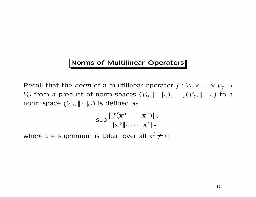
Norms of Multilinear Operators

Recall that the norm of a multilinear operator f : Vα× · · · × Vγ →Vω from a product of norm spaces (Vα, ‖ · ‖α), . . . , (Vγ, ‖ · ‖γ) to a

norm space (Vω, ‖ · ‖ω) is defined as

sup‖f(xα, . . . ,xγ)‖ω

‖xα‖α · · · ‖xγ‖γ

where the supremum is taken over all xi 6= 0.

15

Relation with spectral norm

Define spectral norm of a tensor A ∈ Rd1×···×dk by

‖A‖σ := sup|A(x1, . . . ,xk)|‖x1‖2 · · · ‖xk‖2

.

Note that this differs from the Frobenius norm,

‖A‖F :=(∑d1

i1=1· · ·

∑dk

ik=1|ai1···ik|

2)1/2

for A = Jai1···ikK ∈ Rd1×···×dk.

Proposition. Let A ∈ Rd1×···×dk. The largest singular value of A

equals its spectral norm,

σmax(A) = ‖A‖σ.

16

Hyperdeterminant

Theorem (Gelfand, Kapranov, Zelevinsky, 1992).

R(d1+1)×···×(dk+1) has a non-trivial hyperdeterminant iff

dj ≤∑

i6=jdi

for all j = 1, . . . , k.

For Rm×n, the condition becomes m ≤ n and n ≤ m — that’s

why matrix determinants are only defined for square matrices.

17

Relation with hyperdeterminant

Assume

di − 1 ≤∑

j 6=i(dj − 1)

for all i = 1, . . . , k. Let A ∈ Rd1×···×dk. Easy to see that

A(Id1,u2,u3, . . . ,uk) = 0,

A(u1, Id2,u3, . . . ,uk) = 0,

...

A(u1,u2, . . . ,uk−1, Idk) = 0.

has a solution (u1, . . . ,uk) ∈ Sd1−1 × · · · × Sdk−1 iff

∆(A) = 0

where ∆ is the hyperdeterminant in Rd1×···×dk.

In other words, ∆(A) = 0 iff 0 is a singular value of A.

18

Homogeneous system of multilinear equations

The hyperdeterminant of A = JaijkK ∈ R2×2×2 is

∆(A) := (a2000a2

111 + a2001a2

110 + a2010a2

101 + a2011a2

100)

− 2(a000a001a110a111 + a000a010a101a111 + a000a011a100a111

+ a001a010a101a110 + a001a011a110a100 + a010a011a101a100)

+ 4(a000a011a101a110 + a001a010a100a111).

Result that parallels matrix case: the system of bilinear equations

a000x0y0 + a010x0y1 + a100x1y0 + a110x1y1 = 0,

a001x0y0 + a011x0y1 + a101x1y0 + a111x1y1 = 0,

a000x0z0 + a001x0z1 + a100x1z0 + a101x1z1 = 0,

a010x0z0 + a011x0z1 + a110x1z0 + a111x1z1 = 0,

a000y0z0 + a001y0z1 + a010y1z0 + a011y1z1 = 0,

a100y0z0 + a101y0z1 + a110y1z0 + a111y1z1 = 0.

has a non-trivial solution iff ∆(A) = 0.19

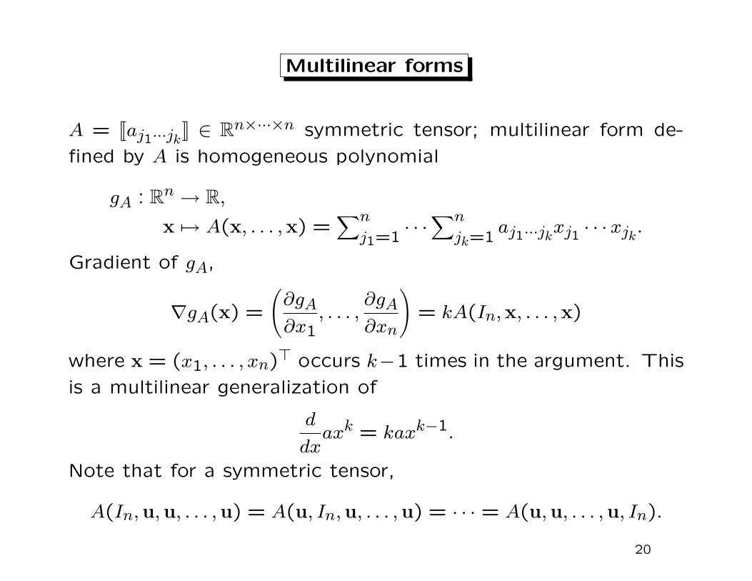
Multilinear forms

A = Jaj1···jkK ∈ Rn×···×n symmetric tensor; multilinear form de-

fined by A is homogeneous polynomial

gA : Rn → R,

x 7→ A(x, . . . ,x) =∑n

j1=1· · ·

∑n

jk=1aj1···jkxj1 · · ·xjk.

Gradient of gA,

∇gA(x) =

(∂gA

∂x1, . . . ,

∂gA

∂xn

)= kA(In,x, . . . ,x)

where x = (x1, . . . , xn)> occurs k−1 times in the argument. This

is a multilinear generalization of

d

dxaxk = kaxk−1.

Note that for a symmetric tensor,

A(In,u,u, . . . ,u) = A(u, In,u, . . . ,u) = · · · = A(u,u, . . . ,u, In).

20

`2-eigenvalues of a symmetric tensor

In this case, the Lagrangian is

L(x, λ) = A(x, . . . ,x)− λ(‖x‖k2 − 1)

Then ∇xL = 0 yields

kA(In,x, . . . ,x) = kλ‖x‖k−22 x,

or, equivalently

A

(In,

x

‖x‖2, . . . ,

x

‖x‖2

)= λ

x

‖x‖2.

∇λL = 0 yields ‖x‖2 = 1. Normalize to get u = x/‖x‖2 ∈ Sn−1,

giving

A(In,u,u, . . . ,u) = λu.

u ∈ Sn−1 will be called an `2-eigenvector and λ will be called an

`2-eigenvalue of A.

21

`2-eigenvalues of a nonsymmetric tensor

How about eigenvalues and eigenvectors for A ∈ Rn×···×n that

may not be symmetric? Even in the order-2 case, the critical

values/points of the Rayleigh quotient no longer gives the eigen-

pairs.

However, as in the order-2 case, eigenvalues and eigenvectors

can still be defined via

A(In,v1,v1, . . . ,v1) = µv1.

Except that now, the equations

A(In,v1,v1, . . . ,v1) = µ1v1,

A(v2, In,v2, . . . ,v2) = µ2v2,

...

A(vk,vk, . . . ,vk, In) = µkvk,

are distinct.22

We will call vi ∈ Rn an mode-i eigenvector and µi an mode-i

eigenvalue. This is just the order-k generalization of left- and

right-eigenvectors for nonsymmetric matrices.

Note that the unit-norm constraint on `2-eigenvectors cannot

be omitted for order 3 or higher because of the lack of scale

invariance.

Characteristic polynomial

Let A ∈ Rn×n. One way to get the characteristic polynomial

pA(λ) = det(A− λI) is as follows.∑n

j=1aijxj = λxi, i = 1, . . . , n,

x21 + · · ·+ x2

n = 1.

System of n+1 polynomial equations in n+1 variables, x1, . . . , xn, λ.

Use Elimination Theory to eliminate all variables x1, . . . , xn, leav-

ing a one-variable polynomial in λ — a simple case of the mul-

tivariate resultant.

The det(A − λI) definition does not generalize to higher order

but the elimination theoretic approach does.

23

Multilinear characteristic polynomial

Let A ∈ Rn×···×n, not necessarily symmetric. Use mode-1 for

illustration.

A(In,x1,x1, . . . ,x1) = µx1.

and the unit-norm condition gives a system of n + 1 equations

in n + 1 variables x1, . . . , xn, λ:∑n

j2=1. . .

∑n

jk=1aij2···jkxj2 · · ·xjk = λxi, i = 1, . . . , n,

x21 + · · ·+ x2

n = 1.

Apply elimination theory to obtain the multipolynomial resultant

or multivariate resultant — a one-variable polynomial pA(λ). Ef-

ficient algorithms exist:

D. Manocha and J.F. Canny, “Multipolynomial resultant algo-

rithms,” J. Symbolic Comput., 15 (1993), no. 2, pp. 99–122.

24

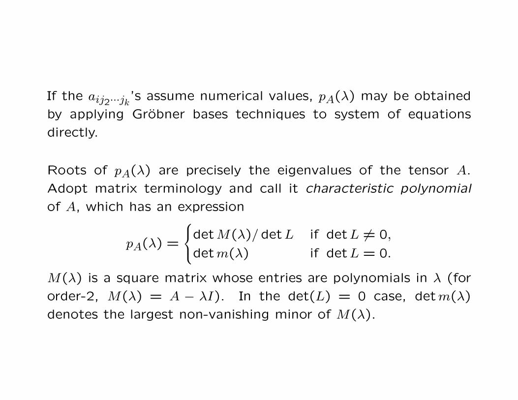
If the aij2···jk’s assume numerical values, pA(λ) may be obtained

by applying Grobner bases techniques to system of equations

directly.

Roots of pA(λ) are precisely the eigenvalues of the tensor A.

Adopt matrix terminology and call it characteristic polynomial

of A, which has an expression

pA(λ) =

detM(λ)/detL if detL 6= 0,

detm(λ) if detL = 0.

M(λ) is a square matrix whose entries are polynomials in λ (for

order-2, M(λ) = A − λI). In the det(L) = 0 case, detm(λ)

denotes the largest non-vanishing minor of M(λ).

Polynomial matrix eigenvalue problem

The matrix M(λ) (or m(λ) in the det(L) = 0 case) allows numer-

ical linear algebra to be used in the computations of eigenvectors

as ∑n

j2=1. . .

∑n

jk=1aij2···jkxj2 · · ·xjk = λxi, i = 1, . . . , n,

x21 + · · ·+ x2

n = 1.

may be reexpressed in the form

M(λ)(1, x1, . . . xn, . . . , xnn)> = (0, . . . ,0)>.

So if (x, λ) is an eigenpair of A. Then M(λ) must have a non-

trivial kernel.

Observe that M(λ) may be expressed as

M(λ) = M0 + M1λ + · · ·+ Mdλd

where Mi’s are matrices with numerical entries.25

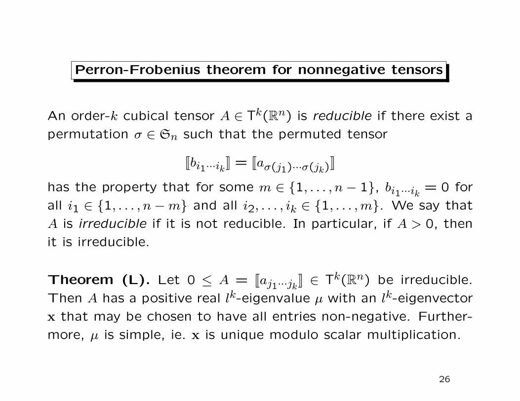
Perron-Frobenius theorem for nonnegative tensors

An order-k cubical tensor A ∈ Tk(Rn) is reducible if there exist a

permutation σ ∈ Sn such that the permuted tensor

Jbi1···ikK = Jaσ(j1)···σ(jk)K

has the property that for some m ∈ {1, . . . , n− 1}, bi1···ik = 0 for

all i1 ∈ {1, . . . , n−m} and all i2, . . . , ik ∈ {1, . . . , m}. We say that

A is irreducible if it is not reducible. In particular, if A > 0, then

it is irreducible.

Theorem (L). Let 0 ≤ A = Jaj1···jkK ∈ Tk(Rn) be irreducible.

Then A has a positive real lk-eigenvalue µ with an lk-eigenvector

x that may be chosen to have all entries non-negative. Further-

more, µ is simple, ie. x is unique modulo scalar multiplication.

26

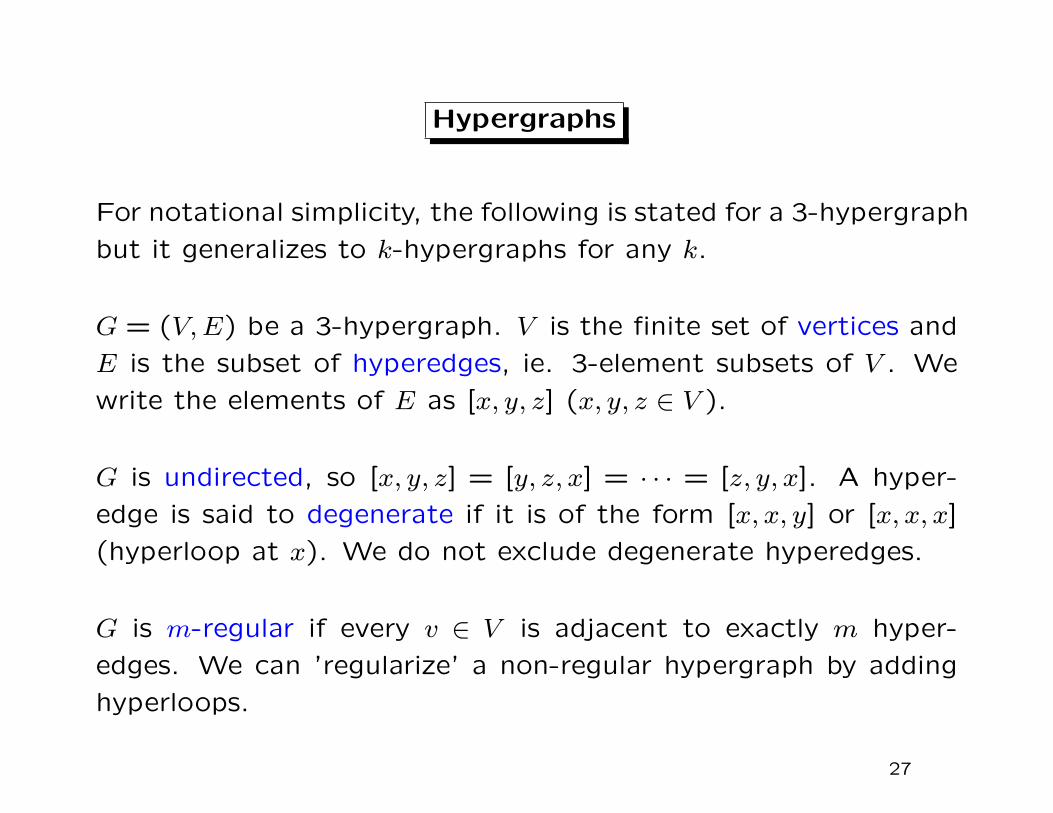
Hypergraphs

For notational simplicity, the following is stated for a 3-hypergraph

but it generalizes to k-hypergraphs for any k.

G = (V, E) be a 3-hypergraph. V is the finite set of vertices and

E is the subset of hyperedges, ie. 3-element subsets of V . We

write the elements of E as [x, y, z] (x, y, z ∈ V ).

G is undirected, so [x, y, z] = [y, z, x] = · · · = [z, y, x]. A hyper-

edge is said to degenerate if it is of the form [x, x, y] or [x, x, x]

(hyperloop at x). We do not exclude degenerate hyperedges.

G is m-regular if every v ∈ V is adjacent to exactly m hyper-

edges. We can ’regularize’ a non-regular hypergraph by adding

hyperloops.

27

Adjacency tensor of a hypergraph

Define the order-3 adjacency tensor A by

Axyz =

1 if [x, y, z] ∈ E,

0 otherwise.

Note that A is |V |-by-|V |-by-|V | nonnegative symmetric tensor.

Consider cubic form A(f, f, f) =∑

x,y,z Axyzf(x)f(y)f(z) (note

that f is a vector of dimension |V |).

Call critical values and critical points of A(f, f, f) constrained

to the set∑

x f(x)3 = 1 (like the `3-norm except we do not

take absolute value) the `3-eigenvalues and `3-eigenvectors of A

respectively.

28

Very basic spectral hypergraph theory I

As in the case of spectral graph theory, combinatorial/topological

properties of a k-hypergraph may be deduced from `k-eigenvalues

of its adjacency tensor (henceforth, in the context of a k-hypergraph,

an eigenvalue will always mean an `k-eigenvalue).

Straightforward generalization of a basic result in spectral graph

theory:

Theorem (Drineas, L). Let G be an m-regular 3-hypergraph

and A be its adjacency tensor. Then

(a) m is an eigenvalue of A;

(b) if µ is an eigenvalue of A, then |µ| ≤ m;

(c) µ has multiplicity 1 if and only if G is connected.

29

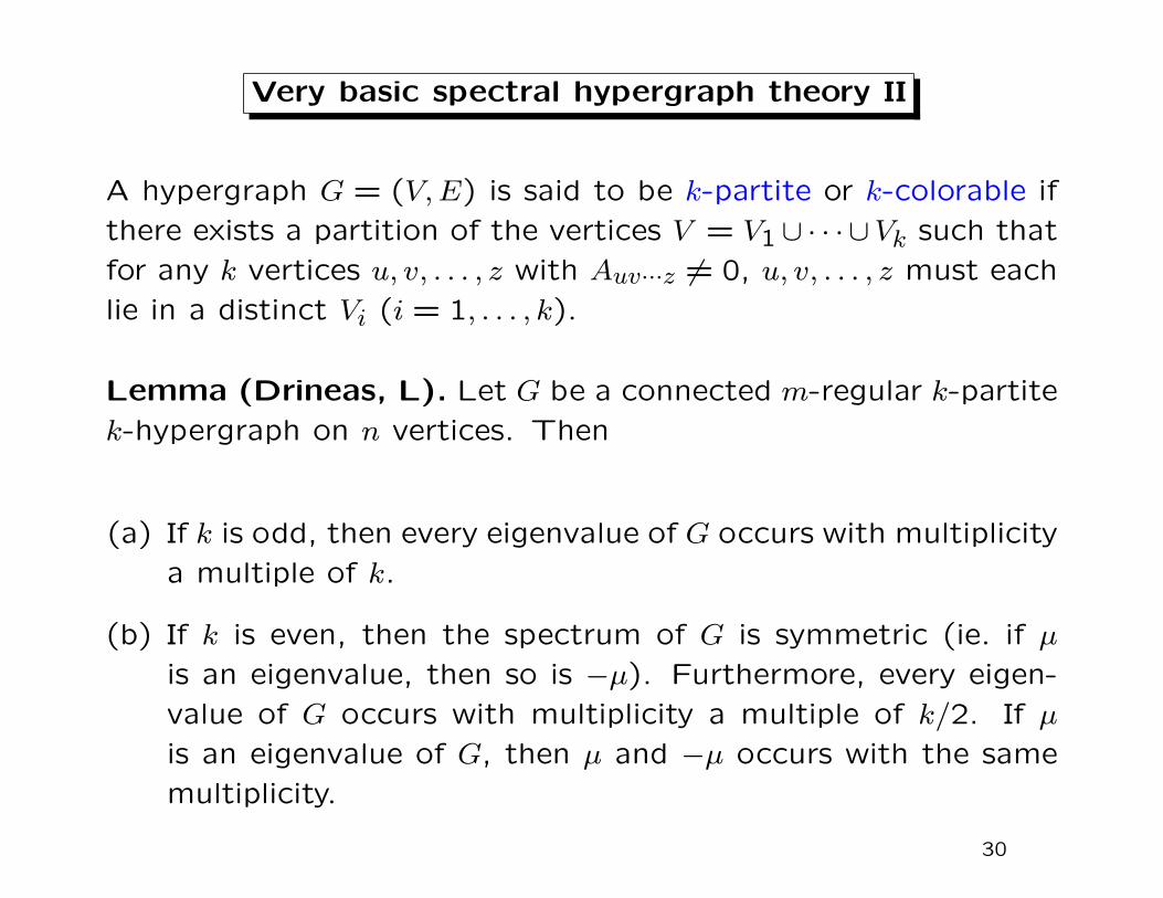
Very basic spectral hypergraph theory II

A hypergraph G = (V, E) is said to be k-partite or k-colorable if

there exists a partition of the vertices V = V1∪ · · · ∪Vk such that

for any k vertices u, v, . . . , z with Auv···z 6= 0, u, v, . . . , z must each

lie in a distinct Vi (i = 1, . . . , k).

Lemma (Drineas, L). Let G be a connected m-regular k-partite

k-hypergraph on n vertices. Then

(a) If k is odd, then every eigenvalue of G occurs with multiplicity

a multiple of k.

(b) If k is even, then the spectrum of G is symmetric (ie. if µ

is an eigenvalue, then so is −µ). Furthermore, every eigen-

value of G occurs with multiplicity a multiple of k/2. If µ

is an eigenvalue of G, then µ and −µ occurs with the same

multiplicity.

30

Liqun Qi’s work

L. Qi, “Eigenvalues of a real supersymmetric tensor,” J. Sym-

bolic Comput., 40 (2005), no. 6, pp. 1302–1324.

(a) Gershgorin circle theorem for `k-eigenvalues;

(b) characterizing positive definiteness of even-ordered forms

(e.g. quartic forms) using `k-eigenvalues;

(c) generalization of trace-sum equality for `2-eigenvalues;

(d) six open conjectures.

See also work by Qi’s postdocs and students: Yiju Wang, Guyan

Ni, Fei Wang.

31

References

http://www-sccm.stanford.edu/nf-publications-tech.html

[dSL] V. de Silva and L.-H. Lim, “Tensor rank and the ill-posedness of thebest low-rank approximation problem,” SIAM J. Matrix Anal. Appl., to appear.

[CGLM2] P. Comon, G. Golub, L.-H. Lim, and B. Mourrain, “Symmetrictensors and symmetric tensor rank,” SCCM Tech. Rep., 06-02, 2006.

[CGLM1] P. Comon, B. Mourrain, L.-H. Lim, and G.H. Golub, “Genericityand rank deficiency of high order symmetric tensors,” Proc. IEEE Int. Con-ference on Acoustics, Speech, and Signal Processing (ICASSP), 31 (2006),no. 3, pp. 125–128.

[L] L.-H. Lim, “Singular values and eigenvalues of tensors: a variationalapproach,” Proc. IEEE Int. Workshop on Computational Advances in Multi-Sensor Adaptive Processing (CAMSAP), 1 (2005), pp. 129–132.

32