multilinear algebra

ELEMENTS OF LINEAR AND MULTILINEAR

ALGEBRA

John M. Erdman

Portland State University

Version April 17, 2011

c©2010 John M. Erdman

E-mail address: [email protected]

Contents

PREFACE vii

NOTATION AND TERMINOLOGY 1Some Algebraic Objects 1Notation for Sets of Numbers 2

Chapter 1. VECTOR SPACES 31.1. Abelian Groups 31.2. Functions and Diagrams 41.3. Rings 71.4. Vector Spaces 81.5. Subspaces 101.6. Linear Combinations and Linear Independence 121.7. Bases for Vector Spaces 14

Chapter 2. LINEAR TRANSFORMATIONS 192.1. Linearity 192.2. Invertible Linear Maps 212.3. Matrix Representations 212.4. Spans, Independence, and Linearity 222.5. Dual Spaces 232.6. Annihilators 25

Chapter 3. THE LANGUAGE OF CATEGORIES 273.1. Objects and Morphisms 273.2. Functors 283.3. Universal Mapping Properties 303.4. Products and Coproducts 313.5. Quotients 323.6. Exact Sequences 333.7. Some Miscellaneous Results 35

Chapter 4. The Spectral Theorem for Vector Spaces 374.1. Projections 374.2. Algebras 384.3. Quotients and Unitizations 404.4. The Spectrum 404.5. Polynomials 414.6. Minimal Polynomials 434.7. Invariant Subspaces 454.8. Burnside’s Theorem 464.9. Eigenvalues and Eigenvectors 474.10. The Spectral Theorem - Vector Space Version 494.11. Two Decomposition Theorems 50

iii

iv CONTENTS

Chapter 5. THE SPECTRAL THEOREM FOR INNER PRODUCT SPACES 535.1. Inner Products 535.2. Orthogonality 555.3. Involutions and Adjoints 585.4. Orthogonal Projections 605.5. The Spectral Theorem for Inner Product Spaces 62

Chapter 6. A BRIEF REVIEW OF DIFFERENTIAL CALCULUS 656.1. Tangency 656.2. The Differential 666.3. The Gradient of a Scalar Field in Rn 68

Chapter 7. MULTILINEAR MAPS AND DETERMINANTS 717.1. Permutations 717.2. Multilinear Maps 717.3. Determinants 727.4. Tensor Products of Vector Spaces 747.5. Tensor Products of Linear Maps 76

Chapter 8. TENSOR ALGEBRAS 778.1. Grassmann Algebras 778.2. Existence of Grassmann Algebras 788.3. The Hodge ∗-operator 80

Chapter 9. DIFFERENTIAL MANIFOLDS 819.1. Manifolds in R3 819.2. Charts, Atlases, and Manifolds 819.3. Differentiable Functions Between Manifolds 839.4. The Geometric Tangent Space 849.5. The Algebraic Tangent Space 87

Chapter 10. DIFFERENTIAL FORMS ON MANIFOLDS 9510.1. Vector Fields 9510.2. Differential 1-forms 9610.3. Differential k-forms 9610.4. Some Classical Vector Analysis 9810.5. Closed and Exact Forms 9910.6. Poincare’s Lemma 99

Chapter 11. HOMOLOGY AND COHOMOLOGY 10311.1. The de Rham Cohomology Group 10311.2. Cochain Complexes 10411.3. Simplicial Homology 10511.4. Simplicial Cohomology 108

Chapter 12. STOKES’ THEOREM 11112.1. Integration of Differential Forms 11112.2. Generalized Stokes’ Theorem 113

Chapter 13. CLIFFORD ALGEBRAS 11713.1. Quadratic Forms 11713.2. Definition of Clifford Algebra 11713.3. Orthogonality with Respect to Bilinear Forms 11813.4. Examples of Clifford Algebras 118

CONTENTS v

Bibliography 121

Index 123

PREFACE

This set of notes is an activity-oriented introduction to the study of linear and multilinearalgebra. The great majority of the results in beginning linear and multilinear are straightforwardand can be verified by the thoughtful student. Indeed, that is the main point of these notes—to convince the beginner that the subject is accessible. In the material that follows there arenumerous indicators that suggest activity on the part of the reader: words such as “proposition”,“example”, “exercise”, and “corollary”, if not followed by a proof or a reference to a proof, areinvitations to verify the assertions made. When the proof of a theorem appears to me to be toodifficult for the average student to (re)invent and I have no improvements to offer to the standardproofs, I provide references to standard treatments. These notes were written for a 2-term course inlinear/multilinear algebra for seniors and first year graduate students at Portland State University.

The prerequisites for working through this material are quite modest. Elementary propertiesof the real number system, the arithmetic of matrices, ability to solve systems of linear equations,and the ability to evaluate the determinant of a square matrix are assumed. A few examples andexercises depend on differentiation and/or integration of real valued functions, but no particularskill with either is required.

There are of course a number of advantages and disadvantages in consigning a document toelectronic life. One advantage is the rapidity with which links implement cross-references. Huntingabout in a book for lemma 3.14.23 can be time-consuming (especially when an author engages inthe entirely logical but utterly infuriating practice of numbering lemmas, propositions, theorems,corollaries, and so on, separately). A perhaps more substantial advantage is the ability to correcterrors, add missing bits, clarify opaque arguments, and remedy infelicities of style in a timelyfashion. The correlative disadvantage is that a reader returning to the web page after a shorttime may find everything (pages, definitions, theorems, sections) numbered differently. (LATEXis anamazing tool.) I will change the date on the title page to inform the reader of the date of the lastnontrivial update (that is, one that affects numbers or cross-references).

The most serious disadvantage of electronic life is impermanence. In most cases when a webpage vanishes so, for all practical purposes, does the information it contains. For this reason (andthe fact that I want this material to be freely available to anyone who wants it) I am making use ofa “Share Alike” license from Creative Commons. It is my hope that anyone who finds this materialuseful will correct what is wrong, add what is missing, and improve what is clumsy. For moreinformation on creative commons licenses see http://creativecommons.org/. Concerning the textitself, please send corrections, suggestions, complaints, and all other comments to the author at

[email protected]

vii

NOTATION AND TERMINOLOGY

Some Algebraic Objects

Let S be a nonempty set. Consider the following axioms:

(1) +: S × S → S. ( + is a binary operation, called addition, on S)(2) (x+ y) + z = x+ (y + z) for all x, y, z ∈ S. (associativity of addition)(3) There exists 0S ∈ S such that x + 0S = 0S + x = x for all x ∈ S. (existence of an

additive identity)(4) For every x ∈ S there exists −x ∈ S such that x+ (−x) = (−x) + x = 0S . (existence

of additive inverses)(5) x+ y = y + x for all x, y ∈ S. (commutativity of addition)(6) · : S × S → S : (x, y) 7→ x · y. (the map (x, y) 7→ x · y is a binary operation, called

multiplication, on S. Convention: We will usually write xy instead of x · y.)(7) (xy)z = x(yz) for all x, y, z ∈ S. (associativity of multiplication)(8) (x+y)z = xz+yz and x(y+z) = xy+xz for all x, y, z ∈ S. (multiplication distributes

over addition)(9) There exists 1S in S such that x1S = 1S x = x for all x ∈ S. (existence of a

multiplicative identity or unit)(10) 1S 6= 0S .(11) For every x ∈ S such that x 6= 0S there exists x−1 ∈ S such that xx−1 = x−1x = 1S .

(existence of multiplicative inverses)(12) xy = yx for all x, y ∈ S. (commutativity of multiplication)

Definitions.

• (S,+) is a semigroup if it satisfies axioms (1)–(2).• (S,+) is a monoid if it satisfies axioms (1)–(3).• (S,+) is a group if it satisfies axioms (1)–(4).• (S,+) is an Abelian group if it satisfies axioms (1)–(5).• (S,+,m) is a ring if it satisfies axioms (1)–(8).• (S,+,m) is a commutative ring if it satisfies axioms (1)–(8) and (12).• (S,+,m) is a unital ring (or ring with identity, or unitary ring) if it satisfies

axioms (1)–(9).• (S,+,m) is a division ring (or skew field) if it satisfies axioms (1)–(11).• (S,+,m) is a field if it satisfies axioms (1)–(12).

Remarks.

• A binary operation is often written additively, (x, y) 7→ x + y, if it is commutative andmultiplicatively, (x, y) 7→ xy, if it is not. This is by no means always the case: in acommutative ring (the real numbers or the complex numbers, for example), both additionand multiplication are commutative.• When no confusion is likely to result we often write 0 for 0S and 1 for 1S .• Many authors require a ring to satisfy axioms (1)–(9).

1

2 NOTATION AND TERMINOLOGY

• It is easy to see that axiom (10) holds in any unital ring except the trivial ring S = {0}.Convention: Unless the contrary is stated we will assume that every unital ring is non-trivial.

Notation for Sets of Numbers

Here is a list of fairly standard notations for some sets of numbers which occur frequently inthese notes:

C is the set of complex numbers

R is the set of real numbers

Rn is the set of all n-tuples (r1, r2, . . . , rn) of real numbers

R+ = {x ∈ R : x ≥ 0}, the positive real numbers

Q is the set of rational numbers

Q+ = {x ∈ Q : x ≥ 0}, the positive rational numbers

Z is the set of integers

Z+ = {0, 1, 2, . . . }, the positive integers

N = {1, 2, 3, . . . }, the set of natural numbers

Nn = {1, 2, 3, . . . , n} the first n natural numbers

[a, b] = {x ∈ R : a ≤ x ≤ b}[a, b) = {x ∈ R : a ≤ x < b}(a, b] = {x ∈ R : a < x ≤ b}(a, b) = {x ∈ R : a < x < b}[a,∞) = {x ∈ R : a ≤ x}(a,∞) = {x ∈ R : a < x}(−∞, b] = {x ∈ R : x ≤ b}(−∞, b) = {x ∈ R : x < b}S1 = {(x, y) ∈ R2 : x2 + y2 = 1}, the unit circle

CHAPTER 1

VECTOR SPACES

1.1. Abelian Groups

1.1.1. Convention. In general, Abelian groups are written additively. That is, the usual notationfor the binary operation on an Abelian group is +. Of course, there are special examples wherethis notation is inappropriate: most notably for the nonzero real numbers, the strictly positive realnumbers, and the nonzero complex numbers under multiplication. It is conventional, if not entirelylogical to write, “let G be an Abelian group,” when what is meant is, “let (G,+) be an Abeliangroup.”

1.1.2. Proposition. The identity element in an Abelian group is unique.

Hint for proof . Let G be an Abelian group. Suppose that there are elements 0 and 0 in G suchthat x+ 0 = x and x+ 0 = x hold for every x ∈ G. Prove that 0 = 0.

1.1.3. Proposition. Each element in an Abelian group has a unique.inverse.

Hint for proof . Let G be an Abelian group and x ∈ G. To prove uniqueness of the inverse forx suppose that there are elements y and z in G such that x + y = 0 and x + z = 0. Prove thaty = z.

1.1.4. Proposition. If x is an element of an Abelian group such that x+ x = x, then x = 0.

1.1.5. Proposition. For every element x in an Abelian group −(−x) = x.

1.1.6. Example. Let S be a nonempty set and F be a field. Denote by F(S,F) the family of allF-valued functions on S. For f , g ∈ F(S,F) define f + g by

(f + g)(x) = f(x) + g(x)

for all x ∈ S. Under this operation (called pointwise addition) F(S,F) is an Abelian group.

1.1.7. Example. As a special case of example 1.1.6, we may regard Euclidean n-space Rn as anAbelian group.

1.1.8. Example. As a special case of example 1.1.6, we may regard the set R∞ of all sequencesof real numbers as an Abelian group.

1.1.9. Example. Let E2 be the Euclidean plane. It contains points (which do not have coordinates)and lines (which do not have equations). A directed segment is an ordered pair of points. Definetwo directed segments to be equivalent if they are congruent (have the same length), lie on parallellines, and have the same direction. This is clearly an equivalence relation on the set DS of directed

segments in the plane. We denote by−−→PQ the equivalence class containing the directed segment

(P,Q), going from the point P to the point Q. Define an operation + on these equivalence classesby

−−→PQ+

−−→QR =

−→PR.

This operation is well defined and under it DS is an Abelian group.

1.1.10. Exercise. Suppose that A, B, C, and D are points in the plane such that−−→AB =

−−→CD.

Show that−→AC =

−−→BD.

3

4 1. VECTOR SPACES

1.1.11. Definition. Let G and H be Abelian groups. A map f : G→ H is a homomorphism if

f(x+ y) = f(x) + f(y)

for all x, y ∈ G. We will denote by Hom(G,H) the set of all homomorphisms from G into H andwill abbreviate Hom(G,G) to Hom(G).

1.1.12. Proposition. If f : G→ H is a homomorphism of Abelian groups, then f(0) = 0.

1.1.13. Proposition. If f : G → H is a homomorphism of Abelian groups, then f(−x) = −f(x)for each x ∈ G.

1.1.14. Definition. Let G and H be Abelian groups. For f and g in Hom(G,H) we define

f + g : G→ H : x 7→ f(x) + g(x).

1.1.15. Example. Let G and H be Abelian groups. With addition as defined in 1.1.14 Hom(G,H)is an Abelian group.

1.1.16. Convention. Let G, H, and J be Abelian groups and f : G → H and g : H → J behomomorphisms. Then the composite of g with f is denoted by gf (rather than by g ◦ f). That is,

gf : G→ J : x 7→ g(f(x)).

1.1.17. Proposition. Let G, H, and J be Abelian groups, f ∈ Hom(G,H), and g ∈ Hom(H,J),then the composite gf belongs to Hom(G, J).

1.2. Functions and Diagrams

1.2.1. Definition. Let S and T be sets and f : S → T . The set S is the domain of f . The setT is the codomain of f . And {(x, f(x)) : x ∈ S} is the graph of f . The domain of f is denotedby dom f .

1.2.2. Definition. A function f is injective (or one-to-one) if x = y whenever f(x) = f(y).That is, f is injective if no two distinct elements in its domain have the same image. An injectivemap is called an injection.

A function is surjective (or onto) if its range is equal to its codomain. A surjective map iscalled a surjection.

A function is bijective (or a one-to-one correspondence) if it is both injective and sur-jective. A bijective map is called a bijection.

1.2.3. Definition. It is frequently useful to think of functions as arrows in diagrams. For example,the situation h : R → S, j : R → T , k : S → U , f : T → U may be represented by the followingdiagram.

S Uk

//

R

S

h

��

R Tj // T

U

f

��

The diagram is said to commute if k ◦ h = f ◦ j. Diagrams need not be rectangular. For instance,

S Uk

//

R

S

h

��

R

U

d

��

is a commutative diagram if d = k ◦ h.

1.2. FUNCTIONS AND DIAGRAMS 5

1.2.4. Example. Here is one diagrammatic way of stating the associative law for composition offunctions: If h : R → S, g : S → T , and f : T → U and we define j and k so that the triangles inthe diagram

S Uk

//

R

S

h

��

R Tj // T

U

f

��S

T

g

??

commute, then the square also commutes.

1.2.5. Convention. If S, T , and U are sets we will often not distinguish between (S × T ) × U ,S × (T × U), and S × T × U . That is, the ordered pairs

((s, t), u

)and

(s, (t, u)

)and the ordered

triple (s, t, u) will usually be treated as identical.

1.2.6. Notation. Let S be a set. The map

idS : S → S : x 7→ x

is the identity function on S. When no confusion will result we write id for idS .

1.2.7. Definition. Let S and T be sets, f : S → T , and A ⊆ S. Then the restriction of f toA, denoted by f

∣∣A

, is the function f ◦ ιA,S , where ιA,S : A → S : x 7→ x is the inclusion map of A

into S. That is, f∣∣A

is the mapping from A into T whose value at each x in A is f(x).

A Tf∣∣A

//

S

A

OO

ιA,S

S

T

f

��

Suppose that g : A→ T and A ⊆ S. A function f : S → T is an extension of g to S if f∣∣A

= g,that is, if the diagram

A Tg//

S

A

OO

ιA,S

S

T

f

��

commutes.

1.2.8. Notation. If S, T , and U are nonempty sets and if f : S → T and g : S → U , then wedefine the function (f, g) : S → T × U by

(f, g)(s) = (f(s), g(s)).

Suppose, on the other hand, that we are given a function h mapping S into the Cartesian productT ×U . Then for each s ∈ S the image h(s) is an ordered pair, which we will write as

(h1(s), h2(s)

).

(The superscripts have nothing to do with powers.) Notice that we now have functions h1 : S → Tand h2 : S → U . These are the components of h. In abbreviated notation h = (h1, h2).

1.2.9. Notation. Let f : S → U and g : T → V be functions between sets. Then f × g denotesthe map

f × g : S × T → U × V : (s, t) 7→(f(s), g(t)

).

6 1. VECTOR SPACES

1.2.10. Exercise. Let S be a set and a : S × S → S be a function such that the diagram

S × S × Sa×id //

id×a// S × S a // S (D1)

commutes. What is (S, a)? Hint. Interpret a as, for example, addition (or multiplication).

1.2.11. Convention. We will have use for a standard one-element set, which, if we wish, we canregard as the Cartesian product of an empty family of sets. We will denote it by 1. For each setS there is exactly one function from S into 1. We will denote it by εS . If no confusion is likely toarise we write ε for εS .

1.2.12. Exercise. Let S be a set and suppose that a : S×S → S and η : 1→ S are functions suchthat both diagram (D1) above and the diagram (D2) which follows commute.

1× S S × Sη×id

// S × S S × 1ooid×η

S

1× S

99

f

S

S × S

OO

a

S

S × 1

ee

g

(D2)

(Here f and g are the obvious bijections.) What is (S, a, η)?

1.2.13. Notation. We denote by δ the diagonal mapping of a set S into S × S. That is,

δ : S → S × S : s 7→ (s, s).

1.2.14. Exercise. Let S be a set and suppose that a : S × S → S and η : 1 → S are functionssuch that the diagrams (D1) and (D2) above commute. Suppose further that there is a functionι : S → S for which the following diagram commutes.

Sδ //

ε

$$

S × Sι×id //

id×ι// S × S a // S

1

η

:: (D3)

What is (S, a, η, ι)?

1.2.15. Notation. Let S be a set. We denote by σ the interchange (or switching) operationon the S × S. That is,

σ : S × S → S × S : (s, t) 7→ (t, s).

1.2.16. Exercise. Let S be a set and suppose that a : S × S → S, η : 1 → S, and ι : S → S arefunctions such that the diagrams (D1), (D2), and (D3) above commute. Suppose further that thefollowing diagram commutes.

S × S

S

a

��

S × S S × Sσ // S × S

S

a

��(D4)

What is (S, a, η, ι, σ)?

1.3. RINGS 7

1.2.17. Exercise. Let f : G→ H be a function between Abelian groups. Suppose that the diagram

G Hf

//

G×G

G

+

��

G×G H ×Hf×f // H ×H

H

+

��

commutes. What can be said about the function f?

1.2.18. Notation. If S and T are sets we denote by F(S, T ) the family of all functions from Sinto T . When F is a field there are several common notations for the family of F-valued functionson S. We denote by l(S) (or by l(S,F), or by FS , or by F(S,F), or by F(S)) the family of allfunctions α : S → F. For x ∈ l(S) we frequently write the value of x at s ∈ S as xs rather thanx(s). (Sometimes it seems a good idea to reduce the number of parentheses cluttering a page.)

The support of a function f : S → F, denoted by supp(f), is {x ∈ S : f(x) 6= 0}.Furthermore, we will denote by lc(S) (or by lc(S,F), or by Fc(S)) the family of all functions

α : S → F with finite support; that is, those functions on S which are nonzero at only finitely manyelements of S.

1.2.19. Exercise. Let S be a set with exactly one element. Discuss the cardinality of (that is, thenumber of elements in) the sets F(∅, ∅), F(∅, S),F(S, ∅), and F(S, S),

1.3. Rings

Recall that an ordered triple (R,+, ·) is a ring if (R,+) is an Abelian group, (R, ·) is a semigroup,and the distributive laws (see Some Algebraic Objects 8) hold. The ring is unital if, in addition,(R \ {0}, ·) is a monoid.

1.3.1. Proposition. The additive identity of a ring is an annihilator. That is, for every elementa of a ring 0a = a0 = 0.

1.3.2. Proposition. If a and b are elements of a ring, then (−a)b = a(−b) = −(ab) and(−a)(−b) = ab.

1.3.3. Proposition. Let a and b be elements of a unital ring. Then 1−ab is invertible if and onlyif 1− ba is.

Hint for proof . Look at the product of 1− ba and 1 + bca where c is the inverse of 1− ab.

1.3.4. Definition. An element a of a ring is left cancellable if ab = ac implies that b = c. Itis right cancellable if ba = ca implies that b = c. A ring has the cancellation property ifevery nonzero element of the ring is both left and right cancellable.

1.3.5. Exercise. Every division ring has the cancellation property.

1.3.6. Definition. A nonzero element a of a ring is a zero divisor (or divisor of zero) if thereexists a nonzero element b of the ring such that (i) ab = 0 or (ii) ba = 0.

Most everyone agrees that a nonzero element a of a ring is a left divisor of zero if it satisfies (i)for some nonzero b and a right divisor of zero if it satisfies (ii) for some nonzero b. There agreementon terminology ceases. Some authors ([5], for example) use the definition above for divisor of zero;others ([13], for example) require a divisor of zero to be both a left and a right divisor of zero; andyet others ([14], for example) avoid the issue entirely by defining zero divisors only for commutativerings. Palmer in [20] makes the most systematic distinctions: a zero divisor is defined as above;an element which is both a left and a right zero divisor is a two-sided zero divisor ; and if the samenonzero b makes both (i) and (ii) hold a is a joint zero divisor.

8 1. VECTOR SPACES

1.3.7. Proposition. A division ring has no zero divisors. That is, if ab = 0 in a division ring,then a = 0 or b = 0.

1.3.8. Proposition. A ring has the cancellation property if and only if it has no zero divisors.

1.3.9. Example. Let G be an Abelian group. Then Hom(G) is a unital ring (under the operationsof addition and composition).

1.3.10. Definition. A function f : R→ S between rings is a (ring) homomorphism if

f(x+ y) = f(x) + f(y) (1.1)

andf(xy) = f(x)f(y) (1.2)

for all x and y in R. If in addition R and S are unital rings and

f(1R) = 1S (1.3)

then f is a unital (ring) homomorphism.Obviously a ring homomorphism f : R→ S is a group homomorphism of R and S regarded as

Abelian groups. The kernel of f as a ring homomorphism is the kernel of f as a homomorphismof Abelian groups; that is ker f = {x ∈ R : f(x) = 0}.

If f−1 exists and is also a ring homomorphism, then f is an isomorphism from R to S. If anisomorphism from R to S exists, then R and S are isomorphic.

1.4. Vector Spaces

1.4.1. Definition. Let F be a field. An ordered triple (V,+,M) is a vector space over F if(V,+) is an Abelian group and M : F → Hom(V ) is a unital ring homomorphism. An element ofV is a vector and an element of F is a scalar. A vector space whose scalars are real numbers isa real vector space and one with complex numbers as scalars is a complex vector space.The vector space {0} containing a single element is the trivial vector space.

1.4.2. Exercise. The definition of vector space found in many elementary texts is something likethe following: a vector space is a set V together with operations of addition and scalar multiplicationwhich satisfy the following axioms:

(1) if x, y ∈ V , then x + y ∈ V ;(2) (x + y) + z = x + (y + z) for every x, y, z ∈ V (associativity);(3) there exists 0 ∈ V such that x + 0 = x for every x ∈ V (existence of additive identity);(4) for every x ∈ V there exists −x ∈ V such that x + (−x) = 0 (existence of additive

inverses);(5) x + y = y + x for every x, y ∈ V (commutativity);(6) if α ∈ F and x ∈ V , then αx ∈ V ;(7) α(x + y) = αx + αy for every α ∈ F and every x, y ∈ V ;(8) (α+ β)x = αx + βx for every α, β ∈ F and every x ∈ V ;(9) (αβ)x = α(βx) for every α, β ∈ F and every x ∈ V ; and

(10) 1 x = x for every x ∈ V .

Verify that this definition is equivalent to the one given above in 1.4.1.

1.4.3. Proposition. If x is an element of a vector space, then (−1)x is the additive inverse of x.That is, (−1)x = −x. (Here, of course, 1 is the multiplicative identity of the field F.)

1.4.4. Example. Let F be a field. Then F can be regarded as a vector space over itself.

1.4.5. Example. Let S be a nonempty set and F be a field. In example 1.1.6 we saw that the familyF(S,F) of F-valued functions on S is an Abelian group under pointwise addition. For f ∈ F(S,F)and α ∈ F define αf by

(αf)(x) = α · f(x)

1.4. VECTOR SPACES 9

for all x ∈ S. Under this operation (called pointwise scalar multiplication) the Abelian groupF(S,F) becomes a vector space. When F = R we write F(S) for F(S,R).

1.4.6. Example. As a special case of example 1.4.5, we may regard Euclidean n-space Rn as avector space.

1.4.7. Example. As another special case of example 1.4.5, we may regard the set R∞ of allsequences of real numbers as a vector space.

1.4.8. Example. Yet another special case of example 1.4.5, is the vector space Mm×n(F) of m×nmatrices of members of F (where m, n ∈ N). We will use Mn(F) as shorthand for Mn×n(F) andMn for Mn(R).

1.4.9. Exercise. Let V be the set of all real numbers. Define an operation of “addition” by

x� y = the maximum of x and y

for all x, y ∈ V . Define an operation of “scalar multiplication” by

α� x = αx

for all α ∈ R and x ∈ V . Prove or disprove: under the operations � and � the set V is a vectorspace.

1.4.10. Exercise. Let V be the set of all real numbers x such that x > 0. Define an operation of“addition” by

x� y = xy

for all x, y ∈ V . Define an operation of “scalar multiplication” by

α� x = xα

for all α ∈ R and x ∈ V . Prove or disprove: under the operations � and � the set V is a vectorspace.

1.4.11. Exercise. Let V be R2, the set of all ordered pairs (x, y) of real numbers. Define anoperation of “addition” by

(u, v)� (x, y) = (u+ x+ 1, v + y + 1)

for all (u, v) and (x, y) in V . Define an operation of “scalar multiplication” by

α� (x, y) = (αx, αy)

for all α ∈ R and (x, y) ∈ V . Prove or disprove: under the operations � and � the set V is a vectorspace.

1.4.12. Exercise. Let V be the set of all n× n matrices of real numbers. Define an operation of“addition” by

A�B = 12(AB +BA)

for all A, B ∈ V . Define an operation of “scalar multiplication” by

α�A = 0

for all α ∈ R and A ∈ V . Prove or disprove: under the operations � and � the set V is a vectorspace. (If you have forgotten how to multiply matrices, look in any beginning linear algebra text.)

1.4.13. Proposition. If x is a vector and α is a scalar, then αx = 0 if and only if α = 0 or x = 0.

In example 1.1.9 we saw how to make the family of equivalence classes of directed segments inthe plane into an Abelian group. We may also define scalar multiplication on these equivalenceclasses by declaring that

(1) if α > 0, then α−−→PQ =

−→PR where P , Q, and R are collinear, P does not lie between Q and

R, and the length of the directed segment (P,R) is α times the length of (P,Q);

10 1. VECTOR SPACES

(2) if α = 0, then α−−→PQ =

−−→PP ; and

(3) if α < 0, then α−−→PQ =

−→PR where P , Q, and R are collinear, P does lie between Q and R,

and the length of the directed segment (R,P ) is α times the length of (P,Q).

1.4.14. Exercise. Show that the scalar multiplication presented above is well-defined and thatit makes the Abelian group of equivalence classes of directed segments in the plane into a vectorspace.

1.4.15. Remark. Among the methods for proving elementary facts about Euclidean geometry ofthe plane three of the most common are synthetic geometry, analytic geometry, and vector geometry.In synthetic geometry points do not have coordinates, lines do not have equations, and vectorsare not mentioned; but standard theorems from Euclid’s Elements are used. Analytic geometrymakes use of a coordinate system in terms of which points are assigned coordinates and lines aredescribed by equations; little or no use is made of vectors or major theorems of Euclidean geometry.Vector geometry uses vectors as defined in the preceding exercise, but does not rely on Euclideantheorems or coordinate systems. Although there is nothing illogical about mixing these methods inestablishing a result, it is interesting to try to construct separate proofs of some elementary resultsusing each method in turn. That is what the next four exercises are about.

1.4.16. Exercise. Use each of the three geometric methods described above to show that thediagonals of a parallelogram bisect each other.

1.4.17. Exercise. Use each of the three geometric methods described above to show that if thediagonals of a quadrilateral bisect each other then the quadrilateral is a parallelogram.

1.4.18. Exercise. Use each of the three geometric methods described above to show that the linejoining the midpoints of the non-parallel sides of a trapezoid is parallel to the bases and its lengthis half the sum of the lengths of the bases.

1.4.19. Exercise. Use each of the three geometric methods described above to show that the linesegments joining the midpoints of adjacent sides of an arbitrary quadrilateral form a parallelogram.

1.4.20. Exercise. Three vertices of a parallelogram PQRS in 3-space are P = (1, 3, 2), Q =(4, 5, 3), and R = (2,−1, 0). What are the coordinates of the point S, opposite Q?

1.5. Subspaces

1.5.1. Definition. A subset M of a vector space V is a subspace of V if it is a vector space underthe operations it inherits from V .

1.5.2. Notation. For a vector space V we will write M � V to indicate that M is a subspaceof V . To distinguish this concept from other uses of the word “subspace” (topological subspace, forexample) writers frequently use the expressions linear subspace, vector subspace, or linear manifold.

1.5.3. Proposition. A nonempty subset of M of a vector space V is a subspace of V if and onlyif it is closed under addition and scalar multiplication. (That is: if x and y belong to M , so doesx + y; and if x belongs to M and α ∈ F, then αx belongs to M .

1.5.4. Example. In each of the following cases prove or disprove that the set of points (x, y, z) inR3 satisfying the indicated condition is a subspace of R3.

(a) x+ 2y − 3z = 4.

(b)x− 1

2=y + 2

3=z

4.

(c) x+ y + z = 0 and x− y + z = 1.(d) x = −z and x = z.(e) x2 + y2 = z.

(f)x

2=y − 3

5.

1.5. SUBSPACES 11

1.5.5. Proposition. Let M be a family of subspaces of a vector space V . Then the intersection⋂M of this family is itself a subspace of V .

1.5.6. Exercise. Let A be a nonempty set of vectors in a vector space V . Explain carefully why itmakes sense to say that the intersection of the family of all subspaces containing A is “the smallestsubspace of V which contains A”.

1.5.7. Exercise. Find and describe geometrically the smallest subspace of R3 containing thevectors (0,−3, 6) and (0, 1,−2).

1.5.8. Exercise. Find and describe geometrically the smallest subspace of R3 containing thevectors (2,−3,−3) and (0, 3, 2).

1.5.9. Example. Let R∞ denote the vector space of all sequences of real numbers. (See exam-ple 1.4.5.) In each of the following a subset of R∞ is described. Prove or disprove that it is asubspace of R∞.

(a) Sequences that have infinitely many zeros (for example, (1, 1, 0, 1, 1, 0, 1, 1, 0, . . . )).(b) Sequences which are eventually zero. (A sequence (xk) is eventually zero if there is an

index n0 such that xn = 0 whenever n ≥ n0.)(c) Sequences that are absolutely summable. (A sequence (xk) is absolutely summable if∑∞

k=1|xk| <∞.)(d) Bounded sequences. (A sequence (xk) is bounded if there is a positive number M such

that |xk| ≤M for every k.)(e) Decreasing sequences. (A sequence (xk) is decreasing if xn+1 ≤ xn for each n.)(f) Convergent sequences. (A sequence (xk) is convergent if there is a number ` such that the

sequence is eventually in every neighborhood of `; that is, if there is a number ` such thatfor every ε > 0 there exists n0 ∈ N such that |xn − ell| < ε whenever n ≥ n0.)

(g) Arithmetic progressions. (A sequence (xk) is arithmetic if it is of the form (a, a+ k,a+ 2k, a+ 3k, . . . ) for some constant k.)

(h) Geometric progressions. (A sequence (xk) is geometric if it is of the form (a, ka, k2a, k3a, . . . )for some constant k.)

1.5.10. Notation. Here are some frequently encountered families of functions:

F = F [a, b] = {f : f is a real valued function on the interval [a, b]} (1.4)

P = P[a, b] = {p : p is a polynomial function on [a, b]} (1.5)

P4 = P4[a, b] = {p ∈ P : the degree of p is less than 4} (1.6)

Q4 = Q4[a, b] = {p ∈ P : the degree of p is equal to 4} (1.7)

C = C[a, b] = {f ∈ F : f is continuous} (1.8)

D = D[a, b] = {f ∈ F : f is differentiable} (1.9)

K = K[a, b] = {f ∈ F : f is a constant function} (1.10)

B = B[a, b] = {f ∈ F : f is bounded} (1.11)

J = J [a, b] = {f ∈ F : f is integrable} (1.12)

(A function f ∈ F is bounded if there exists a number M ≥ 0 such that |f(x)| ≤ M for all x in

[a, b]. It is (Riemann) integrable if it is bounded and∫ ba f(x) dx exists.)

1.5.11. Exercise. For a fixed interval [a, b], which sets of functions in the list 1.5.10 are vectorsubspaces of which?

1.5.12. Notation. If A and B are subsets of a vector space then the sum of A and B, denoted byA+B, is defined by

A+B := {a+ b : a ∈ A and b ∈ B}.

12 1. VECTOR SPACES

The set A−B is defined similarly. For a set {a} containing a single element we write a+B insteadof {a}+B.

1.5.13. Exercise. Let M and N be subspaces of a vector space V . Consider the following subsetsof V .

(1) M ∪N . (A vector v belongs to M ∪N if it belongs to either M or N .)(2) M +N .(3) M \N (A vector v belongs to M \N if it belongs to M but not to N .)(4) M −N .

For each of the sets (a)–(d) above, either prove that it is a subspace of V or give a counterexampleto show that it need not be a subspace of V .

1.5.14. Definition. Let M and N be subspaces of a vector space V . If M ∩ N = {0} andM +N = V , then V is the (internal) direct sum of M and N . In this case we write

V = M ⊕N.In this case the subspaces M and N are complementary and each is the complement of theother.

1.5.15. Example. In R3 let M be the line x = y = z, N be the line x = 12y = 1

3z, and L = M+N .Then L = M ⊕N .

1.5.16. Example. Let M be the plane x + y + z = 0 and N be the line x = y = z in R3. ThenR3 = M ⊕N .

1.5.17. Example. Let C = C[−1, 1] be the vector space of all continuous real valued functionson the interval [−1, 1]. A function f in C is even if f(−x) = f(x) for all x ∈ [−1, 1]; it is oddif f(−x) = −f(x) for all x ∈ [−1, 1]. Let Co = {f ∈ C : f is odd } and Ce = {f ∈ C : f is even }.Then C = Co ⊕ Ce.

1.5.18. Example. Let C = C[0, 1] be the family of continuous real valued functions on the inter-val [0, 1]. Define

f1(t) = t and f2(t) = t4

for 0 ≤ t ≤ 1. Let M be the set of all functions of the form αf1 + βf2 where α, β ∈ R. And let Nbe the set of all functions g in C which satisfy∫ 1

0tg(t) dt = 0 and

∫ 1

0t4g(t) dt = 0.

Then C = M ⊕N .

1.5.19. Exercise. In the preceding example let g(t) = t2 for 0 ≤ t ≤ 1. Find polynomials f ∈ Mand h ∈ N such that f = g + h.

1.5.20. Theorem (Vector Decomposition Theorem). Let V be a vector space such that V = M⊕N .Then for every vector v ∈ V there exist unique vectors m ∈M and n ∈ N such that v = m+ n.

1.5.21. Exercise. Define what it means for a vector space V to be the direct sum of subspacesM1, . . . , Mn. Show (using your definition) that if V is the direct sum of these subspaces, then forevery v ∈ V there exist unique vectors mk ∈Mk (for k = 1, . . . , n) such that v = m1 + · · ·+mn.

1.6. Linear Combinations and Linear Independence

Some authors of linear algebra texts make it appear as if the terms linear dependence and linearindependence, span, and basis pertain only to finite sets of vectors. This is misleading. The termsshould make sense for arbitrary sets. In particular, do not be misled into believing that a basis fora vector space must be a finite set of vectors (or a sequence of vectors).

1.6. LINEAR COMBINATIONS AND LINEAR INDEPENDENCE 13

1.6.1. Definition. A vector y is a linear combination of vectors x1, . . . , xn if there existscalars α1, . . .αn such that y =

∑nk=1 αkxk. Note: linear combinations are finite sums. The linear

combination∑n

k=1 αkxk is trivial if all the coefficients α1, . . .αn are zero. If at least one αk isdifferent from zero, the linear combination is nontrivial.

1.6.2. Example. In R2 the vector (8, 2) is a linear combination of the vectors (1, 1) and (1,−1).

1.6.3. Example. In R3 the vector (1, 2, 3) is not a linear combination of the vectors (1, 1, 0) and(1,−1, 0).

1.6.4. Definition. Let A be a subset of a vector space V . The span of A is the intersection of thefamily of all subspaces of V which contain A. It is denoted by span(A) (or by spanF(A) if we wishto emphasize the role of the scalar field F). The subset A spans the space V if V = span(A). Inthis case we also say that A is a spanning set for V .

1.6.5. Proposition. If A is a nonempty subset of a vector space V , then spanA is the set of alllinear combinations of elements of A.

1.6.6. Remark. Occasionally one must consider the not-too-interesting question of what is meantby the span of the empty set. According to the “abstract” definition 1.6.4 above it is the intersectionof all the subspaces which contain the empty set. That is, span ∅ = {0}. (Had we preferredproposition 1.6.5 as a more “constructive” definition of span—the set of all linear combinations ofelements in ∅—then the span of the empty set would have been just ∅ itself.)

1.6.7. Example. For each n = 0, 1, 2, . . . define a function pn on R by pn(x) = xn. Let P be theset of polynomial functions on R. It is a subspace of the vector space of continuous functions on R.Then P = span{p0, p1, p2, . . . }. The exponential function exp, whose value at x is ex, is not in thespan of the set {p0, p1, p2 . . . }.

1.6.8. Definition. A subset A (finite or not) of a vector space is linearly dependent if thezero vector 0 can be written as a nontrivial linear combination of elements of A; that is, if thereexist vectors x1, . . . , xn ∈ A and scalars α1, . . . , αn, not all zero, such that

∑nk=1 αkxk = 0. A

subset of a vector space is linearly independent if it is not linearly dependent.

Technically, it is a set of vectors that is linearly dependent or independent. Nevertheless, theseterms are frequently used as if they were properties of the vectors themselves. For instance, ifS = {x1, . . . , xn} is a finite set of vectors in a vector space, you may see the assertions “the set S islinearly independent” and “the vectors x1, . . .xn are linearly independent” used interchangeably.

Supersets of linearly dependent sets are linearly dependent and subsets of linearly independentsets linearly independent.

1.6.9. Proposition. Suppose that V is a vector space and A ⊆ B ⊆ V . If A is linearly dependent,then so is B. Equivalently, if B is linearly independent, then so is A.

1.6.10. Exercise. Let w = (1, 1, 0, 0), x = (1, 0, 1, 0), y = (0, 0, 1, 1), and z = (0, 1, 0, 1).

(a) Show that {w, x, y, z} does not span R4 by finding a vector u in R4 such that u /∈span(w, x, y, z).

(b) Show that {w, x, y, z} is a linearly dependent set of vectors by finding scalars α, β, γ, andδ—not all zero—such that αw + βx+ γy + δz = 0.

(c) Show that {w, x, y, z} is a linearly dependent set by writing z as a linear combination ofw, x, and y.

1.6.11. Example. The (vectors going from the origin to) points on the unit circle in R2 are linearlydependent.

1.6.12. Example. For each n = 0, 1, 2, . . . define a function pn on R by pn(x) = xn. Then the set{p0, p1, p2, . . . } is a linearly independent subset of the vector space of continuous functions on R.

14 1. VECTOR SPACES

1.6.13. Example. In the vector space C[0, π] of continuous functions on the interval [0, π] definethe vectors f , g, and h by

f(x) = x

g(x) = sinx

h(x) = cosx

for 0 ≤ x ≤ π. Then f , g, and h are linearly independent.

1.6.14. Example. In the vector space C[0, π] of continuous functions on [0, π] let f , g, h, and jbe the vectors defined by

f(x) = 1

g(x) = x

h(x) = cosx

j(x) = cos2 x

2

for 0 ≤ x ≤ π. Then f , g, h, and j are linearly dependent.

1.6.15. Exercise. Let a, b, and c be distinct real numbers. Show that the vectors (1, 1, 1), (a, b, c),and (a2, b2, c2) form a linearly independent subset of R3.

1.6.16. Exercise. In the vector space C[0, 1] define the vectors f , g, and h by

f(x) = x

g(x) = ex

h(x) = e−x

for 0 ≤ x ≤ 1. Are f , g, and h linearly independent?

1.6.17. Exercise. Let u = (λ, 1, 0), v = (1, λ, 1), and w = (0, 1, λ). Find all values of λ whichmake {u, v, w} a linearly dependent subset of R3.

1.6.18. Exercise. Suppose that {u, v, w} is a linearly independent set in a vector space V . Showthat the set {u+ v, u+ w, v + w} is linearly independent in V .

1.7. Bases for Vector Spaces

1.7.1. Definition. A set B (finite or not) of vectors in a vector space V is a basis for V if it islinearly independent and spans B.

1.7.2. Example. The vectors e1 = (1, 0, 0), e2 = (0, 1, 0), and e3 = (0, 0, 1) constitute an orderedbasis for the vector space R3. This is the standard basis for R3. In elementary calculus textsthese vectors are usually called i, j, and k, respectively.

More generally, in Rn for 1 ≤ k ≤ n let ek be the n-tuple which is zero in every coordinateexcept the kth coordinate where is value is 1. Then {e1, e2, . . . , en} is the standard basis for Rn.

1.7.3. Example. The space Pn(J) of polynomial functions of degree strictly less than n ∈ N onsome interval J ⊆ R with nonempty interior is a vector space of dimension n. For each positiveinteger n = 0, 1, 2, . . . let pn(t) = tn for all t ∈ J . Then {p0, p1, p2, . . . , pn−1} is a basis for Pn(J).We take this to be the standard basis for Pn(J).

1.7.4. Example. The space P(J) of polynomial functions on some interval J ⊆ R with nonemptyinterior is an infinite dimensional vector space. For each n = 0, 1, 2, . . . define a function pn onJ by pn(x) = xn. Then the set {p0, p1, p2, . . . } is a basis for the vector space P(J) of polynomialfunctions on J . We take this to be the standard basis for P(J).

1.7. BASES FOR VECTOR SPACES 15

1.7.5. Example. Let Mm×n be the vector space of all m × n matrices of real numbers. For1 ≤ i ≤ m and 1 ≤ j ≤ n let Eij be the m × n matrix whose entry in the ith row and jth columnis 1 and all of whose other entries are 0. Then

{Eij : 1 ≤ i ≤ m and 1 ≤ j ≤ n

}is a basis for Mm×n.

1.7.6. Exercise. A 2× 2 matrix

[a bc d

]has zero trace if a+ d = 0. Show that the set of all such

matrices is a subspace of M2×2 and find a basis for it.

1.7.7. Exercise. Let U be the set of all matrices of real numbers of the form

[u −u− x0 x

]and V

be the set of all real matrices of the form

[v 0w −v

]. Find bases for U , V, U + V, and U ∩ V.

To show that every nontrivial vector space has a basis.we need to invoke Zorn’s lemma, a settheoretic assumption which is equivalent to the axiom of choice. To this end we need to knowabout such things as partial orderings, chains, and maximal elements.

1.7.8. Definition. A relation on a set S is a subset of the Cartesian product S × S. If therelation is denoted by ≤, then it is conventional to write x ≤ y (or equivalently, y ≥ x) rather than(x, y) ∈ ≤ .

1.7.9. Definition. A relation ≤ on a set S is reflexive if x ≤ x for all x ∈ S. It is transitiveif x ≤ z whenever x ≤ y and y ≤ z. It is antisymmetric if x = y whenever x ≤ y and y ≤ x.A relation which is reflexive, transitive, and antisymmetric is a partial ordering. A partiallyordered set is a set on which a partial ordering has been defined.

1.7.10. Example. The set R of real numbers is a partially ordered set under the usual relation ≤.

1.7.11. Example. A family A of subsets of a set S is a partially ordered set under the relation ⊆.When A is ordered in this fashion it is said to be ordered by inclusion.

1.7.12. Example. Let F(S) be the family of real valued functions defined on a set S. For f ,g ∈ F(S) write f ≤ g if f(x) ≤ g(x) for every x ∈ S. This is a partial ordering on F(S). It isknown as pointwise ordering.

1.7.13. Definition. Let A be a subset of a partially ordered set S. An element u ∈ S is an upperbound for A if a ≤ u for every a ∈ A. An element m in the partially ordered set S is maximalif there is no element of the set which is strictly greater than m; that is, m is maximal if c = mwhenever c ∈ S and c ≥ m. An element m in S is the largest element of S if m ≥ s for everys ∈ S.

Similarly an element l ∈ S is a lower bound for A if l ≤ a for every a ∈ A. An elementm in the partially ordered set S is minimal if there is no element of the set which is strictly lessthan m; that is, m is minimal if c = m whenever c ∈ S and c ≤ m. An element m in S is thesmallest element of S if m ≤ s for every s ∈ S.

1.7.14. Example. Let S = {a, b, c} be a three-element set. The family P(S) of all subsets of S ispartially ordered by inclusion. Then S is the largest element of P(S)—and, of course, it is also amaximal element of P(S). The family Q(S) of all proper subsets of S has no largest element; butit has three maximal elements {b, c}, {a, c}, and {a, b}.

1.7.15. Proposition. A linearly independent subset of a vector space V is a basis for V if andonly if it is a maximal linearly independent subset.

1.7.16. Proposition. A spanning subset for a nontrivial vector space V is a basis for V if andonly if it is a minimal spanning set for V .

1.7.17. Definition. Let S be a partially ordered set with partial ordering ≤.

16 1. VECTOR SPACES

(1) Elements x and y in S are comparable if either x ≤ y or y ≤ x.(2) If ≤ is a partial ordering with respect to which any two elements of S are comparable, it

is a linear ordering (or a total ordering) and S is a linearly ordered set.(3) A linearly ordered subset of S is a chain in S.

1.7.18. Axiom (Zorn’s lemma). A partially ordered set in which every chain has an upper boundhas a maximal element.

1.7.19. Theorem. Let A be a linearly independent subset of a vector space V . Then there existsa basis for V which contains A.

Hint for proof . Order the set of linearly independent subsets of V which contain A by inclusion.Apply Zorn’s lemma.

1.7.20. Corollary. Every vector space has a basis.

Note that the empty set is a basis for the trivial vector space. (See remark 1.6.6.)

1.7.21. Proposition. Let B be a basis for a vector space V . Every element of V can be writtenin a unique way as a linear combination of elements of B.

1.7.22. Notation. Let B be a basis for a vector space V over a field F and x ∈ V . By thepreceding proposition there exists a unique finite set S of vectors in B and for each element e inS there exists a unique scalar xe such that x =

∑e∈S xee. If we agree to let xe = 0 whenever

e ∈ B \ S, we can just as well write x =∑

e∈B xee. Although this notation may make it appearas if we are summing over an arbitrary, perhaps uncountable, set, the fact of the matter is that allbut finitely many of the terms are zero. The function x : B → F : e 7→ xe has finite support, so no“convergence” problems arise. Treat

∑e∈B xee as a finite sum. Associativity and commutativity

of addition in V make the expression unambiguous.

Notice in the preceding that the symbol “x” ends up denoting two different things: a vector inV and a function in lc(B,F). We show in proposition 2.2.9 that this identification is harmless. It isa good idea to teach yourself to feel comfortable with identifying these two objects whenever youare dealing with a vector space with a basis.

1.7.23. Notation. In finite dimensional vector spaces it is usual to adopt some special notationalconventions. Let V be an n-dimensional vector space with an ordered basis {e1, e2, . . . , en}. Ifx ∈ V , then by proposition 1.7.21 we know that there are unique scalars xe1 , xe2 , . . .xen such that

x =n∑k=1

xek ek.

The notation can be unambiguously simplified by writing

x =

n∑k=1

xk ek.

Since the scalars x1, x2, . . .xn uniquely determine the vector x it has become standard to write

x = (x1, x2, . . . , xn) or x =

x1

x2...xn

.That is, a vector x in a finite dimensional space with an ordered basis may be represented as ann-tuple or as an n × 1-matrix. The first of these is frequently referred to as a row vector and thesecond as a column vector.

Next we verify that every subspace has a complementary subspace.

1.7. BASES FOR VECTOR SPACES 17

1.7.24. Proposition. Let M be a subspace of a vector space V . Then there exists a subspace Nof V such that V = M ⊕N .

1.7.25. Lemma. Let V be a vector space with a finite basis {e1, . . . , en} and let v =∑n

k=1 αkek bea vector in V . If p ∈ Nn and αp 6= 0, then {e1, . . . , ep−1, v, ep+1, . . . , en} is a basis for V .

1.7.26. Proposition. If some basis for a vector space V contains n elements, then every linearlyindependent subset of V with n elements is also a basis. Hint. Suppose {e1, . . . , en} is a basis for Vand {v1, . . . , vn} is linearly independent in V . Start by using exercise 1.7.25 to show that (afterperhaps renumbering the ek’s) the set {v1, e2, . . . , en} is a basis for V .

Hint for proof . Suppose {e1, . . . , en} is a basis for V and {v1, . . . , vn} is linearly independentin V . Start by using lemma 1.7.25 to show that (after perhaps renumbering the ek’s) the set{v1, e2, . . . , en} is a basis for V .

1.7.27. Corollary. If a vector space V has a finite basis B, then every basis for V is finite andcontains the same number of elements as B.

1.7.28. Definition. A vector space is finite dimensional if it has a finite basis and the dimen-sion of the space is the number of elements in this (hence any) basis for the space. The dimensionof a finite dimensional vector space V is denoted by dimV . If the space does not have a finite basis,it is infinite dimensional.

Corollary 1.7.27 can be generalized to arbitrary vector spaces.

1.7.29. Theorem. If B and C are bases for a vector space V , then B and C are cardinallyequivalent; that is, there exists a bijection from B onto C.

Proof. See [22], page 45, Theorem 1.12.

1.7.30. Proposition. Let V be a vector space and suppose that V = U ⊕W . Prove that if Bis a basis for U and C is a basis for W , then B ∪ C is a basis for V . From this conclude thatdimV = dimU + dimW .

1.7.31. Definition. The transpose of an n×n matrix A =[aij]

is the matrix At =[aji]

obtained

by interchanging the rows and columns of A. The matrix A is symmetric if At = A.

1.7.32. Exercise. Let S3 be the vector space of all symmetric 3× 3 matrices of real numbers.

(a) What is the dimension of S3?(b) Find a basis for S3.

CHAPTER 2

LINEAR TRANSFORMATIONS

2.1. Linearity

2.1.1. Definition. Let V and W be vector spaces over the same field F. A function T : V →W islinear if T (x+ y) = Tx+ Ty and T (αx) = αTx for all x, y ∈ V and α ∈ F. For linear functionsit is a matter of convention to write Tx instead of T (x) whenever it does not cause confusion. (Ofcourse, we would not write Tx+y when we intend T (x+y).) Linear functions are frequently calledlinear transformations or linear maps.

2.1.2. Notation. If V and W are vector spaces (over the same field F) the family of all linearfunctions from V into W is denoted by L(V,W ). Linear functions are frequently called lineartransformations, linear maps, or linear mappings. When V = W we condense the notation L(V, V )to L(V ) and we call the members of L(V ) operators.

2.1.3. Example. Let V and W be vector spaces over a field F. For S, T ∈ L(V,W ) define S + Tby

(S + T )(x) := Sx+ Tx

for all x ∈ V . For T ∈ L(V,W ) and α ∈ F define αT by

(αT )(x) := α(Tx)

for all x ∈ V . Under these operations L(V,W ) is a vector space.

2.1.4. Proposition. If S : V → W and T : W → X are linear maps between vector spaces, thenthe composite of these two functions, nearly always written as TS rather than T ◦ S, is a linearmap from V into X.

2.1.5. Convention. If S : V → W and T : W → X are linear maps between vector spaces, thenthe composite linear map of these two functions is nearly always written as TS rather than T ◦ S.In the same vein, T 2 = T ◦ T , T 3 = T ◦ T ◦ T , and so on.

2.1.6. Exercise. Use the notation of definition 1.4.1 and suppose that (V,+,M) and (W,+,M)are vector spaces over a common field F and that T ∈ Hom(V,W ) is such that the diagram

V WT

//

V

V

Mα

��

V WT // W

W

Mα

��

commutes for every α ∈ F. What can be said about the homomorphism T?

2.1.7. Example. Let a < b and C = C([a, b]) be the vector space of all continuous real valuedfunctions on the interval [a, b]. Then integration

T : C → R : f 7→∫ b

af(t) dt

is a linear map.

19

20 2. LINEAR TRANSFORMATIONS

2.1.8. Example. Let a < b and C1 = C1([a, b]) be the set of all continuously differentiable realvalued functions on the interval [a, b]. (Recall that a function is continuously differentiableif it has a derivative and the derivative is continuous.) Then differentiation

D : C1 → C : f 7→ f ′

is linear.

2.1.9. Example. Let R∞ be the vector space of all sequences of real numbers and define

S : R∞ → R∞ : (x1, x2, x3, . . . ) 7→ (0, x1, x2, . . . ).

Then S is a linear operator. It is called the unilateral shift operator.

2.1.10. Definition. Let T : V →W be a linear transformation between vector spaces. Then kerT ,the kernel (or nullspace) of T is defined to be the set of all x in V such that Tx = 0. Also,ranT , the range of T (or the image of T ), is the set of all y in W such that y = Tx for some xin V . The rank of T is the dimension of its range and the nullity of T is the dimension of itskernel.

2.1.11. Definition. Let T : V → W be a linear transformation between vector spaces and let Abe a subset of V . Define T→(A) := {Tx : x ∈ A}. This is the (direct) image of A under T .

2.1.12. Proposition. Let T : V → W be a linear map between vector spaces and M � V . ThenT→(M) is a subspace of W . In particular, the range of a linear map is a subspace of the codomainof the map.

2.1.13. Definition. Let T : V →W be a linear transformation between vector spaces and let B bea subset of W . Define T←(B) := {x ∈ V : Tx ∈ B}. This is the inverse image of B under T .

2.1.14. Proposition. Let T : V → W be a linear map between vector spaces and M � W . ThenT←(M) is a subspace of V . In particular, the kernel of a linear map is a subspace of the domainof the map.

2.1.15. Exercise. Let T : R3 → R3 : x = (x1, x2, x3) 7→ (x1 + 3x2 − 2x3, x1 − 4x3, x1 + 6x2).

(a) Identify the kernel of T by describing it geometrically and by giving its equation(s).(b) Identify the range of T by describing it geometrically and by giving its equation(s).

2.1.16. Exercise. Let T be the linear map from R3 to R3 defined by

T (x, y, z) = (2x+ 6y − 4z, 3x+ 9y − 6z, 4x+ 12y − 8z).

Describe the kernel of T geometrically and give its equation(s). Describe the range of T geometri-cally and give its equation(s).

2.1.17. Exercise. Let C = C[a, b] be the vector space of all continuous real valued functions onthe interval [a, b] and C1 = C1[a, b] be the vector space of all continuously differentiable real valuedfunctions on [a, b]. Let D : C1 → C be the linear transformation defined by

Df = f ′

and let T : C → C1 be the linear transformation defined by

(Tf)(x) =

∫ x

af(t) dt

for all f ∈ C and x ∈ [a, b].

(a) Compute (and simplify) (DTf)(x).(b) Compute (and simplify) (TDf)(x).(c) Find the kernel of T .(d) Find the range of T .

2.1.18. Proposition. A linear map T : V → W between vector spaces is injective if and only ifkerT = {0}.

2.3. MATRIX REPRESENTATIONS 21

2.2. Invertible Linear Maps

2.2.1. Notation. In the sequel we will usually denote the identity operator x 7→ x on a vectorspace V by IV , or just I, rather than by idV .

2.2.2. Definition. A linear map T : V →W between vector spaces is left invertible (or has aleft inverse, or is a section) if there exists a linear map L : W → V such that LT = IV .

The map T is right invertible (or has a right inverse, or is a retraction) if there existsa linear map R : W → V such that TR = IW . We say that T is invertible (or has an inverse,or is an isomorphism) if there exists a linear map T−1 : W → V which is both a left and a rightinverse for T . If there exists an isomorphism between two vector spaces V and W , we say that thespaces are isomorphic and we write V ∼= W .

2.2.3. Exercise. Show that an operator T ∈ L(V ) is invertible if it satisfies the equation

T 2 − T + IV = 0.

2.2.4. Example. The unilateral shift operator S on the vector space R∞ of all sequences of realnumbers (see 2.1.9) is injective but not surjective. It is left invertible but not right invertible.

2.2.5. Proposition. A linear map T : V → W between vector spaces is invertible if and only ifhas both a left inverse and a right inverse.

2.2.6. Proposition. A linear map between vector spaces is invertible if and only if it is bijective.

2.2.7. Proposition. An operator T on a vector space V is invertible if and only if it has a uniqueright inverse.

Hint for proof . Consider ST + S − IV , where S is the unique right inverse for T .

2.2.8. Example. Every n-dimensional real vector space is isomorphic to Rn.

Hint for proof . Recall the notational conventions made in 1.7.23.

2.2.9. Example. Let B be a basis for a vector space V over a field F. Then V ∼= lc(B,F).

Hint for proof . Recall the notational conventions made in 1.7.22.

2.2.10. Proposition. Let S, T ∈ L(V,W ) where V and W are vector spaces over a field F; andlet B be a basis for V . If S(e) = T (e) for every e ∈ B, then S = T .

2.2.11. Proposition. Let V and W be a vector spaces. If V = M ⊕N and T : M →W is a linear

map, then there exists T ∈ L(V,W ) such that T∣∣M

= T and T∣∣N

= 0.

We can now make a considerable improvement on proposition 2.2.6.

2.2.12. Proposition. A linear transformation has a left inverse if and only if it is injective.

2.2.13. Proposition. A linear transformation has a right inverse if and only if it is surjective.

2.2.14. Proposition. Let V and W be vector spaces over a field F and B be a basis for V . Iff : B →W , then there exists a unique linear map Tf : V →W which is an extension of f .

2.2.15. Exercise. Let S be a set, V be a vector space over a field F, and f : S → V be a bijection.Explain how to use f to make S into a vector space isomorphic to V .

2.3. Matrix Representations

2.3.1. Proposition. Let T ∈ L(V,W ) where V is an n-dimensional vector space and W is an m-dimensional vector space and let {e1, e2, . . . , en} be an ordered basis for V . Define an m×n-matrix[T ] whose kth column (1 ≤ k ≤ n) is the column vector Tek (see 1.7.23). Then for each x ∈ V wehave

Tx = [T ]x.


The displayed equation above requires a little interpretation. The left side is T evaluated at x;the right side is an m × n matrix multiplied by an n × 1 matrix (that is, a column vector). Thenthe asserted equality is of two m× 1 matrices (column vectors).

2.3.2. Definition. If V and W are finite dimensional vector spaces with ordered bases and T ∈L(V,W ), then the matrix [T ] in the preceding proposition is the matrix representation of T .

2.3.3. Exercise. Let T : R4 → R3 be defined by

Tx = (x1 − 3x3 + x4, 2x1 + x2 + x3 + x4, 3x2 − 4x3 + 7x4)

for every x = (x1, x2, x3, x4) ∈ R4.

(a) Find [T ].(b) Find T (1,−2, 1, 3).(c) Independently of part (b) calculate the matrix product [T ]

1−213

.(d) Find kerT .(e) Find ranT .

2.3.4. Exercise. Let P4(R) be the vector space of polynomial functions of degree strictly lessthan 4 on R. Consider the linear transformation D2 : P4 → P4 : f 7→ f ′′.

(a) Find the matrix representation of D2 (with respect to the standard basis for P4(R).(b) Find the kernel of D2.(c) Find the range of D2.

2.3.5. Exercise. Let T : P4(R) → P5(R) be the linear transformation defined by (Tp)(t) = (2 +3t)p(t) for every p ∈ P4(R) and t ∈ R. Find the matrix representation of T with respect to thestandard bases for P4(R) and P5(R).

2.3.6. Exercise. Let Pn(R) be the vector space of all polynomial functions on R with degreestrictly less than n. Define T : P3(R)→ P5(R) by

Tf(x) =

∫ x

0

∫ u

0p(t) dt du

for all x, u ∈ R.

(a) Find the matrix representation of the linear map T (with respect to the standard basesfor P3(R) and P5(R)).

(b) Find the kernel of T .(c) Find the range of T .

2.4. Spans, Independence, and Linearity

2.4.1. Proposition. Let T : V →W be a linear map between vector spaces. If A is a subset of Vsuch that T→(A) is linearly independent, then A is linearly independent.

2.4.2. Proposition. Let T : V → W be a linear map between vector spaces. If T is injective andA is a linearly independent subset of V , then T→(A) is a linearly independent subset of W .

2.4.3. Proposition. Let T : V → W be a linear map between vector spaces and A ⊆ V . ThenT→(spanA) = spanT→(A).

2.4.4. Proposition. Let T : V → W be a linear map between vector spaces. If T is injective andB is a basis for a subspace U of V , then T→(B) is a basis for T→(U).

2.4.5. Proposition. Let T : V → W be a linear map between vector spaces. If V is spanned by aset B of vectors and T→(B) is a basis for W , then B is a basis for V and T is an isomorphism.

2.4.6. Exercise. Prove that a linear transformation T : R3 → R2 cannot be one-to-one and thata linear transformation S : R2 → R3 cannot be onto. What is the most general version of theseassertions that you can invent (and prove)?

2.5. DUAL SPACES 23

2.4.7. Proposition. Suppose that V and W are finite dimensional vector spaces of the same finitedimension and that T : V →W is a linear map. Then the following are equivalent;

(a) T is injective;(b) T is surjective; and(c) T is invertible.

2.5. Dual Spaces

2.5.1. Definition. Let V be a vector space over a field F. A linear map f : V → F is a linearfunctional on V . The set of linear functionals on V is denoted by V ∗; that is, V ∗ = L(V,F).The vector space V ∗ is the dual space of V .

2.5.2. Convention. Let B be a basis for a vector space V over a field F. Recall that in 1.7.22 weadopted the notation

x =∑e∈B

xee

where x denotes both an element of V and a scalar valued function on B with finite support. Inexample 2.2.9 we justified this identification by establishing that the vector spaces V and lc(B,F)are isomorphic. Notice that this is an extension of the usual notation in Rn where we write a vectorv in terms of its components:

x =n∑k=1

xk ek.

2.5.3. Exercise. According to convention 2.5.2 above, what is the value of f(e) when e and f areelements of the basis B?

2.5.4. Proposition. Let V be a vector space with basis B. For every v ∈ V define a function v∗

on V by

v∗(x) =∑e∈B

xe ve for all x ∈ V .

Then v∗ is a linear functional on V .

2.5.5. Notation. In the preceding proposition 2.5.4 the value v∗(x) of v∗ at x is often written as〈x, v〉.

2.5.6. Exercise. Consider the notation 2.5.5 above in the special case that the scalar field F = R.Then 〈 , 〉 is an inner product on the vector space V . (For a definition of inner product see 5.1.1,)

2.5.7. Exercise. In the special case that the scalar field F = C, things above are usually done abit differently. For v ∈ V the function v∗ is defined by

v∗(x) = 〈x, v〉 =∑e∈B

xe ve .

Why do you think things are done this way?

2.5.8. Proposition. Let v be a nonzero vector in a vector space V and B be a basis for V whichcontains the vector v. Then there exists a linear functional f ∈ V ∗ such that f(v) = 1 and f(e) = 0for every e ∈ B \ {v}.

2.5.9. Corollary. Let M be a subspace of a vector space V and v a vector in V which does notbelong to M . Then there exists f ∈ V ∗ such that f(v) = 1 and f→(M) = {0}.

2.5.10. Corollary. If v is a vector in a vector space V and f(v) = 0 for every f ∈ V ∗, then v = 0.

2.5.11. Definition. Let F be a field. A family F of F-valued functions on a set S containing atleast two points separates points of S if for every x, y ∈ S such that x 6= y there exists f ∈ Fsuch that f(x) 6= f(y).


2.5.12. Corollary. For every nontrivial vector space V , the dual space V ∗ separates points of V .

2.5.13. Proposition. Let V be a vector space with basis B. The map Φ: V → V ∗ : v 7→ v∗ (seeproposition 2.5.4) is linear and injective.

The next result is the Riesz-Frechet theorem for finite dimensional vector spaces with basis. Itis important to keep in mind that the result does not hold for infinite dimensional vector spaces(see proposition 2.5.18) and that the mapping Φ depends on the basis which has been chosen forthe vector space.

2.5.14. Theorem. Let V be a finite dimensional vector space with basis B. Then the map Φdefined in the preceding proposition 2.5.13 is an isomorphism. Thus for every f ∈ V ∗ there existsa unique vector a ∈ V such that a∗ = f .

2.5.15. Definition. Let V be a vector space with basis {eλ : λ ∈ Λ}. A basis {ελ : λ ∈ Λ} for V ∗

is the dual basis for V ∗ if it satisfies

εµ(eλ) =

{1, if µ = λ;0, if µ 6= λ.

2.5.16. Theorem. Every finite dimensional vector space V with a basis has a unique dual basisfor its dual space. In fact, if {e1, . . . , en} is a basis for V , then {(e1)∗, . . . , (en)∗} is the dual basisfor V ∗.

2.5.17. Corollary. If a vector space V is finite dimensional, then so is its dual space and dimV =dimV ∗.

In proposition 2.5.13 we showed that the map

Φ: V → V ∗ : v 7→ v∗

is always an injective linear map. In corollary 2.5.17 we showed that if V is finite dimensional, thenso is V ∗ and Φ is an isomorphism between V and V ∗. This is never true in infinite dimensionalspaces.

2.5.18. Proposition. If V is infinite dimensional, then Φ is not an isomorphism.

Hint for proof . Let B be a basis for V . Is there a functional g ∈ V ∗ such that g(e) = 1 forevery e ∈ B? Could such a functional be Φ(x) for some x ∈ V ?

2.5.19. Proposition. Let V be a vector space over a field F. For every x in V define

x : V ∗ → F : φ 7→ φ(x) .

(a) The vector x belongs to V ∗∗ for each x ∈ V .(b) Let Γ

Vbe the map from V to V ∗∗ which takes x to x. (When no confusion is likely we

write Γ for ΓV

, so that Γ(x) = x for each x ∈ V .) The function Γ is linear.(c) The function Γ is injective.

2.5.20. Proposition. If V is a finite dimensional vector space, then the map Γ: V → V ∗∗ definedin the preceding proposition 2.5.19 is an isomorphism.

2.5.21. Proposition. If V is infinite dimensional, then the mapping Γ (defined in 2.5.19) is notan isomorphism.

Hint for proof . Let B be a basis for V and ψ ∈ V ∗ be as in proposition 2.5.18. Show that if welet C0 be {e∗ : e ∈ B}, then the set C0 ∪{ψ} is linearly independent and can therefore be extendedto a basis C for V ∗. Find an element τ in V ∗∗ such that τ(ψ) = 1 and τ(φ) = 0 for every otherφ ∈ C. Can τ be Γx for some x ∈ V ?

2.6. ANNIHILATORS 25

2.6. Annihilators

2.6.1. Notation. Let V be a vector space and M ⊆ V . Then

M⊥ := {f ∈ V ∗ : f(x) = 0 for all x ∈M}We say that M⊥ is the annihilator of M . (The reasons for using the familiar “orthogonalcomplement” notation M⊥ (usually read “M perp”) will become apparent when we study innerproduct spaces, where “orthogonality” actually makes sense.)

2.6.2. Exercise. Find the annihilator in(R2)∗

of the vector (1, 1) in R2. (Express your answer in

terms of the standard dual basis for(R2)∗

.)

2.6.3. Proposition. Let M and N be subsets of a vector space V . Then

(a) M⊥ is a subspace of V ∗.(b) If M ⊆ N , then N⊥ �M⊥.(c) (spanM)⊥ = M⊥.(d) (M ∪N)⊥ = M⊥ ∩N⊥.

2.6.4. Proposition. If M and N be subspaces of a vector space V , then

(M +N)⊥ = M⊥ ∩N⊥.

2.6.5. Exercise. Explain why it is necessary in the preceding proposition to assume that M andN are subspaces of V and not just subsets of V .

2.6.6. Notation. Let V be a vector space and F ⊆ V ∗. Then

F⊥ := {x ∈ V : f(x) = 0 for all f ∈ F}We say that F⊥ is the pre-annihilator of F .

2.6.7. Proposition. If M is a subspace of a vector space V , then(M⊥

)⊥ = M .

2.6.8. Exercise. Propositions 2.6.3 and 2.6.4 asserted some properties of the annihilator mappingM 7→ M⊥. See to what extent you can prove similar results about the pre-annihilator mapping

F 7→ F⊥. What can you say about the set(F⊥)⊥

?

2.6.9. Proposition. Let V be a finite dimensional vector space and F be a subspace of V ∗. IfF⊥ = {0}, then F = V ∗.

CHAPTER 3

THE LANGUAGE OF CATEGORIES

3.1. Objects and Morphisms

3.1.1. Definition. Let A be a class, whose members we call objects. For every pair (S, T ) ofobjects we associate a set Mor(S, T ), whose members we call morphisms from S to T . We assumethat Mor(S, T ) and Mor(U, V ) are disjoint unless S = U and T = V .

We suppose further that there is an operation ◦ (called composition) that associates withevery α ∈Mor(S, T ) and every β ∈Mor(T,U) a morphism β ◦ α ∈Mor(S,U) in such a way that:

(1) γ ◦ (β ◦ α) = (γ ◦ β) ◦ α whenever α ∈Mor(S, T ), β ∈Mor(T,U), and γ ∈Mor(U, V );(2) for every object S there is a morphism IS ∈ Mor(S, S) satisfying α ◦ IS = α whenever

α ∈Mor(S, T ) and IS ◦ β = β whenever β ∈Mor(R,S).

Under these circumstances the class A, together with the associated families of morphisms, is acategory.

We will reserve the notation Sα // T for a situation in which S and T are objects in some

category and α is a morphism belonging to Mor(S, T ). As is the case with groups and vector spaceswe usually omit the composition symbol ◦ and write βα for β ◦ α.

3.1.2. Example. The category SET has sets for objects and functions (maps) as morphisms.

3.1.3. Example. The category AbGp has Abelian groups for objects and group homomorphismsas morphisms. (See proposition 1.1.17.)

3.1.4. Example. The category VEC has vector spaces for objects and linear transformations asmorphisms. (See proposition 2.1.4.)

3.1.5. Example. Let S and T be partially ordered sets. A function f : S → T is order preserv-ing if f(x) ≤ f(y) in T whenever x ≤ y in S. The category POSET has partially ordered sets forobjects and order preserving maps as morphisms.

The preceding examples are examples of concrete categories—that is, categories in which theobjects are sets (together, usually, with additional structure) and the morphism are functions(usually preserving, in some sense, this extra structure). In these notes the categories of interestare concrete ones. Even so, it may be of interest to see an example of a category that is notconcrete.

3.1.6. Example. Let G be a monoid. Consider a category CG having exactly one object, whichwe call ?. Since there is only one object there is only one family of morphisms Mor(?, ?), whichwe take to be G. Composition of morphisms is defined to be the monoid multiplication. That is,a ◦ b := ab for all a, b ∈ G. Clearly composition is associative and the identity element of G is theidentity morphism. So CG is a category.

3.1.7. Definition. In any concrete category we will call an injective morphism a monomorphismand a surjective morphism an epimorphism.

3.1.8. CAUTION. The definitions above reflect the original Bourbaki use of the term and arethe ones most commonly adopted by mathematicians outside of category theory where “monomor-phism” means “left cancellable” and “epimorphism” means “right cancellable”. (Notice that the

27

28 3. THE LANGUAGE OF CATEGORIES

terms injective and surjective may not make sense when applied to morphisms in a category thatis not concrete.)

A morphism Bg //C is left cancellable if whenever morphisms A

f1 //B and Af2 //B

satisfy gf1 = gf2, then f1 = f2. Saunders Mac Lane suggested calling left cancellable morphismsmonic morphisms. The distinction between monic morphisms and monomorphisms turns out tobe slight. In these notes almost all of the morphisms we encounter are monic if and only if they aremonomorphisms. As an easy exercise prove that any injective morphism in a (concrete) categoryis monic. The converse sometimes fails.

In the same vein Mac Lane suggested calling a right cancellable morphism (that is, a morphism

Af //B such that whenever morphisms B

g1 //C and Bg2 //C satisfy g1f = g2f , then g1 = g2) an

epic morphism. Again it is an easy exercise to show that in a (concrete) category any epimorphismis epic. The converse, however, fails in some rather common categories.

3.1.9. Definition. The terminology for inverses of morphisms in categories is essentially the same

as for functions. Let Sα // T and T

β // S be morphisms in a category. If β ◦ α = IS , then β is aleft inverse of α and, equivalently, α is a right inverse of β. We say that the morphism α is

an isomorphism (or is invertible) if there exists a morphism Tβ // S which is both a left and

a right inverse for α. Such a function is denoted by α−1 and is called the inverse of α.

3.1.10. Proposition. If a morphism in some category has both a left and a right inverse, then itis invertible.

In any concrete category one can inquire whether every bijective morphism (that is, every mapwhich is both a monomorphism and an epimorphism) is an isomorphism. We saw in proposi-tion 2.2.6 that in the category VEC the answer is yes. In the next example the answer is no.

3.1.11. Example. In the category POSET of partially ordered sets and order preserving mapsnot every bijective morphism is an isomorphism.

3.1.12. Example. If in the category CG of example 3.1.6 the monoid G is a group, then everymorphism in CG is an isomorphism.

3.2. Functors

3.2.1. Definition. If A and B are categories a (covariant) functor F from A to B (written

AF // B) is a pair of maps: an object map F which associates with each object S in A an

object F (S) in B and a morphism map (also denoted by F ) which associates with each morphismf ∈Mor(S, T ) in A a morphism F (f) ∈Mor(F (S), F (T )) in B, in such a way that

(1) F (g ◦ f) = F (g) ◦ F (f) whenever g ◦ f is defined in A; and(2) F (idS) = idF (S) for every object S in A.

The definition of a contravariant functor AF //B differs from the preceding definition

only in that, first, the morphism map associates with each morphism f ∈ Mor(S, T ) in A amorphism F (f) ∈Mor(F (T ), F (S)) in B and, second, condition (1) above is replaced by

(1′) F (g ◦ f) = F (f) ◦ F (g) whenever g ◦ f is defined in A.

3.2.2. Example. A forgetful functor is a functor that maps objects and morphisms from acategory C to a category C′ with less structure or fewer properties. For example, if V is a vectorspace, the functor F which “forgets” about the operation of scalar multiplication on vector spaceswould map V into the category of Abelian groups. (The Abelian group F (V ) would have the sameset of elements as the vector space V and the same operation of addition, but it would have noscalar multiplication.) A linear map T : V → W between vector spaces would be taken by thefunctor F to a group homomorphism F (T ) between the Abelian groups F (V ) and F (W ).

3.2. FUNCTORS 29

Forgetful functor can “forget” about properties as well. If G is an object in the category ofAbelian groups, the functor which “forgets” about commutativity in Abelian groups would take Ginto the category of groups.

It was mentioned in the preceding section that all the categories that are of interest in thesenotes are concrete categories (ones in which the objects are sets with additional structure and themorphisms are maps which preserve, in some sense, this additional structure). We will have severaloccasions to use a special type of forgetful functor—one which forgets about all the structure ofthe objects except the underlying set and which forgets any structure preserving properties of themorphisms. If A is an object in some concrete category C, we denote by �A its underlying set.

And if Af // B is a morphism in C we denote by |f | the map from |A| to |B| regarded simply

as a function between sets. It is easy to see that | | , which takes objects in C to objects in SET(the category of sets and maps) and morphisms in C to morphisms in SET, is a covariant functor.

In the category VEC of vector spaces and linear maps, for example, | | causes a vector space Vto “forget” about both its addition and scalar multiplication (|V | is just a set). And if T : V →Wis a linear transformation, then |T | : |V | → |W | is just a map between sets—it has “forgotten”about preserving the operations.

3.2.3. Notation. Let f : S → T be a function between sets. Then we define f→(A) = {f(x) : x ∈A} and f←(B) = {x ∈ S : f(x) ∈ B}. We say that f→(A) is the image of A under f and thatf←(B) is the preimage of B under f .

3.2.4. Definition. A partially ordered set is order complete if every nonempty subset has asupremum (that is, a least upper bound) and an infimum (a greatest lower bound).

3.2.5. Definition. Let S be a set. Then the power set of S, denoted by P(S), is the family ofall subsets of S.

3.2.6. Example (The power set functors). Let S be a nonempty set.

(a) The power set P(S) of S partially ordered by ⊆ is order complete.(b) The class of order complete partially ordered sets and order preserving maps is a category.

(c) For each function f between sets let P(f) = f→. Then P is a covariant functor from thecategory of sets and functions to the category of order complete partially ordered sets andorder preserving maps.

(d) For each function f between sets let P(f) = f←. Then P is a contravariant functor fromthe category of sets and functions to the category of order complete partially ordered setsand order preserving maps.

3.2.7. Definition. Let T : V → W be a linear map between vector spaces. For every g ∈ W ∗

let T ∗(g) = g T . Notice that T ∗(g) ∈ V ∗. The map T ∗ from the vector space W ∗ into the vectorspace V ∗ is the (vector space) adjoint map of T .

3.2.8. CAUTION. In inner product spaces we will use the same notation T ∗ for a different map.If T : V →W is a linear map between inner product spaces, then the (inner product space) adjointtransformation T ∗ maps W to V (not W ∗ to V ∗).

3.2.9. Example (The vector space duality functor). Let T ∈ L(V,W ) where V and W are vectorspaces over a field F. Then the pair of maps V 7→ V ∗ and T 7→ T ∗ is a contravariant functor fromthe category of vector spaces and linear maps into itself. Show that (the morphism map of) thisfunctor is linear. (That is, show that (S + T )∗ = S∗ + T ∗ and (αT )∗ = αT ∗ for all S, T ∈ L(V,W )and α ∈ F.)

There are several quite different results that in various texts are labeled as the fundamentaltheorem of linear algebra. Many of them seem to me not to be particularly “fundamental” because


they apply only to finite dimensional inner product spaces or, what amounts to the same thing,matrices. I feel the following result deserves the name because it holds for arbitrary linear mapsbetween arbitrary vector spaces.

3.2.10. Theorem (Fundamental Theorem of Linear Algebra). For every linear map T : V → Wbetween vector spaces the following hold.

(1) kerT ∗ = (ranT )⊥;(2) ranT ∗ = (kerT )⊥;(3) kerT = (ranT ∗)⊥; and(4) ranT = (kerT ∗)⊥.

3.2.11. Exercise. What is the relationship between a linear map T being injective and its adjointT ∗ being surjective? between T being surjective and T ∗ being injective?

3.3. Universal Mapping Properties

Much of mathematics involves the construction of new objects from old ones—things suchas products, coproducts, quotients, completions, compactifications, and unitizations. Often it ispossible—and highly desirable—to characterize such a construction by means of a diagram whichdescribes what the constructed object “does” rather than telling what it “is” or how it is con-structed. Such a diagram is a universal mapping diagram and it describes the universalmapping property of the object being constructed.

Here is a first example of such a property.

3.3.1. Definition. Let F be an object in a concrete category C and ι : S → |F | be a map whosedomain is a nonempty set S. We say that the object F is free on the set S (or that F is thefree object generated by S) if for every object A in C and every map f : S → |A| there exists

a unique morphism fι : F → A in C such that |fι| ◦ ι = f .

S |F |ι //S

|A|

f

��

|F |

|A|

|fι|

��

F

A

fι

��

We will be interested in free vector spaces; that is, free objects in the category VEC of vectorspaces and linear maps. Naturally, merely defining a concept does not guarantee its existence. Itturns out, in fact, that free vector spaces exist on arbitrary sets. (See exercise 3.3.5.)

3.3.2. Exercise. In the preceding definition reference to the forgetful functor is often omitted andthe accompanying diagram is often drawn as follows:

S Fι //S

A

f

��

F

A

fι

��

It certainly looks a lot simpler. Why do you suppose I opted for the more complicated version?

3.3.3. Proposition. If two objects in some concrete category are free on the same set, then theyare isomorphic.

3.4. PRODUCTS AND COPRODUCTS 31

3.3.4. Definition. Let A be a subset of a nonempty set S and F be a field. Define χA

: S → F,the characteristic function of A, by

χA

(x) =

{1, if x ∈ A0, otherwise

3.3.5. Example. If S is an arbitrary nonempty set and F is a field, then there exists a vectorspace V over F which is free on S. This vector space is unique (up to isomorphism).

Hint for proof . Given the set S let V be the set of all F-valued functions on S which have finitesupport. Define addition and scalar multiplication pointwise. The map ι : s 7→ χ{s} of each element

s ∈ S to the characteristic function of {s} is the desired injection. To verify that V is free over S it

must be shown that for every vector space W and every function Sf // |W | there exists a unique

linear map Vf //W which makes the following diagram commute.

S |V |ι //S

|W |

f

��

|V |

|W |

|f |

��

V

W

f

��

3.3.6. Proposition. Every vector space is free.

Hint for proof . Of course, part of the problem is to specify a set S on which the given vectorspace is free.

3.3.7. Exercise. Let S = {a, ∗,#}. Then an expression such as

3a− 12 ∗+

√2 #

is said to be a formal linear combination of elements of S. Make sense of such expressions.

3.4. Products and Coproducts

In this section we define products and coproducts of vector spaces in terms of universal mappingproperties.

3.4.1. Definition. Let A1 and A2 be objects in a category C. We say that a triple (P, π1, π2),where P is an object and πk : P → Ak (k = 1, 2) are morphisms, is a product of A1 and A2 iffor every object B in C and every pair of morphisms fk : B → Ak (k = 1, 2) there exists a uniquemap g : B → P such that fk = πk ◦ g for k = 1, 2.

A1 Pooπ1

P A2π2//

B

A1

f1

��

B

P

g

��

B

A2

f2

��

A triple (P, j1, j2), where P is an object and jk : Ak → P , (k = 1, 2) are morphisms, is acoproduct of A1 and A2 if for every object B in C and every pair of morphisms Fk : Ak → B(k = 1, 2) there exists a unique map G : P → B such that Fk = G ◦ jk for k = 1, 2.

A1 Pj1

// P A2oo

j2

B

A1

??

F1

B

P

OO

G

B

A2

__

F2


3.4.2. Proposition. In an arbitrary category products and coproducts (if they exist) are essentiallyunique.

“Essentially unique” means unique up to isomorphism. Thus in the preceding proposition theclaim is that if (P, π1, π2) and (Q, ρ1, ρ2) are both products of two given objects, then P ∼= Q.

3.4.3. Definition. Let V and W be vector spaces over the same field F. To make the Cartesianproduct V ×W into a vector space we define addition by

(v, w) + (v′, w′) = (v + v′, w + w′)

(where v, v′ ∈ V and w, w′ ∈W ), and we define scalar multiplication by

α(v, w) = (αv, αw)

(where α ∈ F, v ∈ V , and w ∈ W ). The resulting vector space we call the (external) directsum of V and W . It is conventional to use the same notation V ⊕W for external direct sums thatwe use for internal direct sums.

3.4.4. Example. The external direct sum of two vector spaces (as defined in 3.4.3) is a vectorspace.

3.4.5. Example. In the category of vector spaces and linear maps the external direct sum is botha product but also a coproduct.

3.4.6. Example. In the category of sets and maps (functions) the product and the coproduct arenot the same.

3.4.7. Proposition. Let U , V , and W be vector spaces. If U ∼= W , then U ⊕ V ∼= W ⊕ V .

3.4.8. Example. The converse of the preceding proposition is not true.

3.4.9. Definition. Let V0, V1, V2, . . . be vector spaces (over the same field). Then their (ex-

ternal) direct sum, which is denoted by∞⊕k=0

Vk, is defined to be the set of all functions

v : Z+ →⋃∞k=0 Vk with finite support such that v(k) = vk ∈ Vk for each k ∈ Z+. The usual

pointwise addition and scalar multiplication make this set into a vector space.

3.5. Quotients

3.5.1. Definition. Let A be an object in a concrete category C. A surjective morphism Aπ //B

in C is a quotient map for A if a function g : B → C (in SET) is a morphism (in C) wheneverg ◦ π is a morphism. An object B in C is a quotient object for A if it is the range of somequotient map for A.

3.5.2. Proposition. In the category of vector spaces and linear maps every surjective linear mapis a quotient map.

The next item shows how a particular quotient object can be generated by “factoring out asubspace”.

3.5.3. Definition. Let M be a subspace of a vector space V . Define an equivalence relation ∼ onV by

x ∼ y if and only if y − x ∈M.

For each x ∈ V let [x] be the equivalence class containing x. Let V/M be the set of all equivalenceclasses of elements of V . For [x] and [y] in V/M define

[x] + [y] := [x+ y]

and for α ∈ R and [x] ∈ V/M defineα[x] := [αx].

3.6. EXACT SEQUENCES 33

Under these operations V/M becomes a vector space. It is the quotient space of V by M . Thenotation V/M is usually read “V mod M”. The linear map

π : V → V/M : x 7→ [x]

is called the quotient map.

3.5.4. Exercise. Verify the assertions made in definition 3.5.3. In particular, show that ∼ is anequivalence relation, that addition and scalar multiplication of the set of equivalence classes is welldefined, that under these operations V/M is a vector space, and that the quotient map is linear.

The following result is called the fundamental quotient theorem or the first isomorphism theoremfor vector spaces.

3.5.5. Theorem. Let V and W be vector spaces and M � V . If T ∈ L(V,W ) and kerT ⊇ M ,

then there exists a unique T ∈ L(V/M ,W ) which makes the following diagram commute.

V

π

��

T

!!V/M

T

// W

Furthermore, T is injective if and only if kerT = M ; and T is surjective if and only if T is.

3.5.6. Corollary. If T : V →W is a linear map between vector spaces, then ranT ∼= V/ kerT .

For obvious reasons the next result is usually called the rank-plus-nullity theorem. (It is alsosometimes listed as part of the fundamental theorem of linear algebra.)

3.5.7. Proposition. Let T : V → W be a linear map between vector spaces. If V is finite dimen-sional, then

rank T + nullity T = dimV.

3.5.8. Corollary. If M is a subspace of a finite dimensional vector space V , then dimV/M =dimV − dimM .

3.6. Exact Sequences

3.6.1. Definition. A sequence of vector spaces and linear maps

· · · // Vn−1jn // Vn

jn+1 // Vn+1// · · ·

is said to be exact at Vn if ran jn = ker jn+1. A sequence is exact if it is exact at each of itsconstituent vector spaces. A sequence of vector spaces and linear maps of the form

0 // Uj // V

k //W // 0

is a short exact sequence. (Here 0 denotes the trivial 0-dimensional vector space, and theunlabeled arrows are the obvious linear maps.)

3.6.2. Proposition. The sequence

0 // Uj // V

k //W // 0

of vector spaces is exact at U if and only if j is injective. It is exact at W if and only if k issurjective.


3.6.3. Exercise. Suppose a < b. Let K be the family of constant functions on the interval [a, b],C1 be the family of all continuously differentiable functions on [a, b], and C be the family of allcontinuous functions on [a, b]. (A function f is said to be continuously differentiable if itsderivative f ′ exists and is continuous.)

Specify linear maps j and k so that the following sequence is short exact:

0 //Kj // C1 k // C // 0.

3.6.4. Exercise. Let C be the family of all continuous functions on the interval [0, 2]. Let E1 bethe mapping from C into R defined by E1(f) = f(1). (The functional E1 is called evaluation at 1.)

Find a subspace F of C such that the following sequence is short exact.

0 // F ι // C E1 // R // 0.

3.6.5. Exercise. If j : U → V is an injective linear map between vector spaces, then the sequence

0 // Uj // V

π // V/ ran j // 0

is exact.

3.6.6. Example. Let U and V be vector spaces. Then the following sequence is short exact:

0 // Uι1 // U ⊕ V π2 // V // 0.

The indicated linear maps are the obvious ones:

ι1 : U → U ⊕ V : u 7→ (u, 0)

and

π2 : U ⊕ V → V : (u, v) 7→ v.

3.6.7. Proposition. Consider the following diagram in the category of vector spaces and linearmaps.

0 //

0

0

0 //

U ′ V ′j ′

//

U

U ′

f

��

U Vj // V

V ′

g

��V ′ W ′

k′//

V

V ′

V Wk // W

W ′

h

��0//

0// 0

0

If the rows are exact and the left square commutes, then there exists a unique linear map h : W →W ′ which makes the right square commute.

3.6.8. Proposition (The Short Five Lemma). Consider the following diagram of vector spacesand linear maps

0 //

0

0

0 //

U ′ V ′j ′

//

U

U ′

f

��

U Vj // V

V ′

g

��V ′ W ′

k′//

V

V ′

V Wk // W

W ′

h

��0//

0// 0

0

where the rows are exact and the squares commute. Then the following hold.

(a) If g is surjective, so is h.(b) If f is surjective and g is injective, then h is injective.(c) If f and h are surjective, so is g.(d) If f and h are injective, so is g.

3.7. SOME MISCELLANEOUS RESULTS 35

3.6.9. Proposition. Show that if 0 //Uj //V

k //W //0 is an exact sequence of vector spacesand linear maps, then V ∼= U ⊕W .

Hint for proof . Consider the following diagram and use proposition 3.6.8.

0 // Uj // V

k //

g

��

W // 0

0 // Ui1// U ⊕W

π2 // W //i2

oo 0

.

The trick is to find the right map g.

3.6.10. Exercise. Prove the converse of the preceding exercise. That is, suppose that U , V , andW are vector spaces and that V ∼= U ⊕W ; prove that there exist linear maps j and k such that the

sequence 0 // Uj // V

k //W // 0 is exact. Hint. Suppose g : U ⊕W → V is an isomorphism.Define j and k in terms of g.

3.6.11. Proposition. Let M and M ′ be subspaces of vector spaces V and V ′, respectively. Provethe following.

(a) Every linear map T : V → V ′ which satisfies T (M) ⊆ M ′ induces a linear map T from

V/M into V ′/M ′ which satisfies T (v +M) = (Tv) +M ′ for all v ∈ V .(b) If T is an isomorphism and T (M) = M ′, then V/M ∼= V ′/M ′.

3.6.12. Proposition. If 0 // Uj // V

k //W // 0 is an exact sequence of vector spaces andlinear maps, then W ∼= V/ ran j. Thus, if U � V and j is the inclusion map, then W ∼= V/U .

Give two different proofs of the preceding result: one using theorem 3.5.5 and the other usingproposition 3.6.13.

3.6.13. Proposition. The converse of proposition 3.6.12 is also true. That is, if j : U → V isan injective linear map between vector spaces and W ∼= V/ ran j, then there exists a linear map k

which makes the sequence 0 // Uj // V

k //W // 0 exact.

3.6.14. Proposition. If V0, V1, . . . , Vn are finite dimensional vector spaces and the sequence

0 // Vndn // Vn−1

// . . . // V1d1 // V0

// 0

is exact, thenn∑k=0

(−1)k dimVk = 0.

3.7. Some Miscellaneous Results

3.7.1. Definition. Let T ∈ L(V,W ), where V and W are vector spaces. Define cokerT , thecokernel of T , to be W/ ranT .

3.7.2. Proposition. Let U , V , and W be vector spaces. If S ∈ L(U, V ), T ∈ L(V,W ), then thesequence

0 // kerS // kerTS // kerT // cokerS // cokerTS // cokerT // 0

is exact.

3.7.3. Proposition. Let W be a vector space and M � V �W . Then

(W/M)/

(V/M) ∼= W/V.

Hint for proof . Proposition 3.6.12.


3.7.4. Proposition. Let V be a vector space and M , M ′ � V Then

(M +M ′)/M ∼= M ′/(M ∩M ′) .

3.7.5. Proposition. Let M be a subspace of a vector space V . Then the following are equivalent:

(a) dimV/M <∞ ;(b) there exists a finite dimensional subspace F of V such that V = M ⊕ F ; and(c) there exists a finite dimensional subspace F of V such that V = M + F .

3.7.6. Exercise. Suppose that a vector space V is the direct sum of subspaces U and W . Someauthors define the codimension of U to be dimW . Others define it to be dimV/U . Show thatthese are equivalent.

CHAPTER 4

The Spectral Theorem for Vector Spaces

4.1. Projections

Much of mathematical research consists analyzing complex objects by writing them as a combi-nation of simpler objects. In the case of vector space operators the simpler objects, the fundamentalbuilding blocks, are projection operators.

4.1.1. Definition. Let V be a vector space. An operator E ∈ L(V ) is a projection operatorif it is idempotent; that is, if E2 = E.

4.1.2. Proposition. If E is a projection operator on a vector space V , then

V = ranE ⊕ kerE.

4.1.3. Proposition. Let V be a vector space and E, F ∈ L(V ). If E +F = IV and EF = 0, thenE and F are projection operators and V = ranE ⊕ ranF .

4.1.4. Proposition. Let V be a vector space and E1, . . . , En ∈ L(V ). If∑n

k=1Ek = IV andEiEj = 0 whenever i 6= j, then each Ek is a projection operator and V =

⊕nk=1 ranEk.

4.1.5. Proposition. If E is a projection operator on a vector space V , then ranE = {x ∈ V : Ex =x}.

4.1.6. Proposition. Let E and F be projection operators on a vector space V . Then E + F = IVif and only if EF = FE = 0 and kerE = ranF .

4.1.7. Definition. Let V be a vector space and suppose that V = M ⊕ N . We know from anearlier theorem 1.5.20 that for each v ∈ V there exist unique vectors m ∈M and n ∈ N such thatv = m + n. Define a function E

NM: V → V by E

NMv = m. The function E

NMis called the

projection of V along N onto M . (This terminology is, of course, optimistic. We must provethat E

NMis in fact a projection operator.)

4.1.8. Proposition. If M⊕N is a direct sum decomposition of a vector space V , then the functionENM

defined in 4.1.7 is a projection operator whose range is M and whose kernel is N .

4.1.9. Proposition. If M ⊕ N is a direct sum decomposition of a vector space V , then ENM

+EMN

= IV and ENM

EMN

= 0.

4.1.10. Proposition. If E is a projection operator on a vector space V , then there exist M , N 4 Vsuch that E = E

NM.

4.1.11. Exercise. Let M be the line y = 2x and N be the y-axis in R2. Find [EMN

] and [ENM

].

4.1.12. Exercise. Let E be the projection of R3 onto the plane 3x− y + 2z = 0 along the z-axis.Find the matrix representation [E] (of E with respect to the standard basis of R3).

4.1.13. Exercise. Let F be the projection of R3 onto the z-axis along the plane 3x− y + 2z = 0.Where does F take the point (4, 5, 1)?

4.1.14. Exercise. Let P be the plane in R3 whose equation is x + 2y − z = 0 and L be the line

whose equations arex

3= y =

z

2. Let E be the projection of R3 along L onto P and F be the

37

38 4. THE SPECTRAL THEOREM FOR VECTOR SPACES

projection of R3 along P onto L. Then

[E] =1

3

a −b c−d d d

a− 2d −b+ 2d c+ 2d

and [F ] =1

3

3d 3e −3dd e −d2d 2e −2d

where a = , b = , c = , d = , and e = .

4.1.15. Exercise. Let T : V →W be linear and S : W → V a left inverse for T . Then

(a) W = ranT ⊕ kerS, and(b) TS is the projection along kerS onto ranT .

4.2. Algebras

4.2.1. Definition. Let (A,+,M) be a vector space over a field F which is equipped with anotherbinary operation · : A × A → A : (a, b) 7→ ab in such a way that (A,+, · ) is a ring. If additionallythe equations

α(ab) = (αa)b = a(αb) (4.1)

hold for all a, b ∈ A and α ∈ F, then (A,+,M, · ) is an algebra over the field F (sometimesreferred to as a linear associative algebra). We abuse notation in the usual way by writingsuch things as, “Let A be an algebra.” We say that an algebra A is unital if its underlying ring(A,+, · ) is. And it is commutative if its ring is.

4.2.2. Example. A field may be regarded as an algebra over itself.

4.2.3. Example. If S is a nonempty set, then the vector space F(S,F) (see example 1.4.5) isa commutative unital algebra under pointwise multiplication, which is defined for all f , g ∈F(S,F) by

(f · g)(s) = f(s) · g(s)

for all s ∈ S. The constant function 1 (that is, the function whose value at each s ∈ S is 1) is themultiplicative identity.

4.2.4. Example. If V is a vector space, then the set L(V ) of linear operators on V is a unitalalgebra under pointwise addition, pointwise scalar multiplication, and composition.

4.2.5. Notation. In the following material we make the notational convention that if B and C aresubsets of (a ring or) an algebra A, then BC denotes the set of all sums of products of elements inB and C. That is

BC := {b1c1 + · · ·+ bncn : n ∈ N; b1, . . . , bn ∈ B; and c1, . . . , cn ∈ C}.

And, of course, if b ∈ A, then bC = {b}C.

4.2.6. Definition. A map f : A → B between algebras is an (algebra) homomorphism if itis a linear map between A and B as vector spaces which preserves multiplication (in the sense ofequation (1.2). In other words, an algebra homomorphism is a linear ring homomorphism. It isa unital (algebra) homomorphism if it preserves identities (as in (1.3)). The kernel of analgebra homomorphism f : A→ B is, of course, {a ∈ A : f(a) = 0}.

If f−1 exists and is also an algebra homomorphism, then f is an isomorphism from A to B.If an isomorphism from A to B exists, then A and B are isomorphic.

Here are three essentially obvious facts about algebra homomorphisms.

4.2.7. Proposition. Every bijective algebra (or ring) homomorphism is an isomorphism.

4.2.8. Proposition. If f : A→ B is an isomorphism between algebras (or rings) and A is unital,then so is B and f is a unital homomorphism.

4.2. ALGEBRAS 39

4.2.9. Proposition. Let A, B, and C be algebras (or rings). If f : A → B and g : B → C arehomomorphisms, so is gf : A→ C. (As is the case with group homomorphism and linear maps, gfdenotes the composite function g ◦ f .) If f and g are unital, so is gf .

Here is an example of another important algebra.

4.2.10. Example. We have seen in example 1.4.8 that the set Mn of n×n matrices of real numbersis a vector space. If a =

[aij]

and b =[bkl]

are n× n matrices of real numbers, then the product

of a and b is the n×n matrix c = ab whose entry in the ith row and kth column is cik =∑n

j=1 aijbjk .This definition makes Mn into a unital algebra.

Hint for proof . Proving associativity of matrix multiplication can be something of a nuisance ifone charges ahead without thinking. As an alternative to brute calculation look at exercise 2.2.15.

4.2.11. Proposition. If φ : A→ B is an algebra homomorphism, then the kernel of φ is an idealin A and the range of φ is a subalgebra of B.

4.2.12. Definition. A subset of an algebra A which is closed under the operations of addition,multiplication, and scalar multiplication is a subalgebra of A. If A is a unital algebra and B is asubalgebra of A which contains the multiplicative identity of A, then B is a unital subalgebraof A.

4.2.13. CAUTION. Be very careful with the preceding definition. It is possible for B to be asubalgebra of an algebra A and to be a unital algebra but still not be a unital subalgebra of A!The definition requires that for B to be a unital subalgebra of A the identity of B must be thesame as the identity of A. Example: Under pointwise operations A = R2 is a unital algebra. Theset B = {(x, 0) : x ∈ R} is a subalgebra of A. And certainly B is unital (the element (1, 0) is themultiplicative identity of B). But B is not a unital subalgebra of A because it does not containthe multiplicative identity (1, 1) of A.

4.2.14. Example. Let S be a nonempty set. The family B(S) of all bounded real valued functionson S is a unital subalgebra of the algebra F(S) of all real valued functions on S.

4.2.15. Definition. A left ideal in an algebra A is a vector subspace J of A such that AJ ⊆ J .(For right ideals, of course, we require JA ⊆ J .) We say that J is an ideal if it is both a leftand a right ideal. A proper ideal is an ideal which is a proper subset of A.

The ideals {0} and A are often referred to as the trivial ideals of A. The algebra A is simpleif it has no nontrivial ideals.

4.2.16. Convention. Whenever we refer to an ideal in an algebra we understand it to be a two-sided ideal (unless the contrary is stated).

4.2.17. Definition. An element a of a unital algebra A is invertible if there exists an elementa−1 ∈ A such that aa−1 = a−1a = 1A.

4.2.18. Proposition. No invertible element in a unital algebra can belong to a proper ideal.

4.2.19. Proposition. Let a be an element of a commutative algebra A. Then aA is an ideal in A.If A is unital and a is not invertible, then aA is a proper ideal in A.

4.2.20. Example. Let J be a family of ideals in an algebra A. Then the⋂J is an ideal in A.

4.2.21. Definition. Let a be an element of an algebra A. Then the intersection of all the idealsof A which contain a is the principal ideal generated by a.

4.2.22. Proposition. Let a be an element of a commutative algebra A. The ideal aA in proposi-tion 4.2.19 is the principal ideal generated by a.


4.3. Quotients and Unitizations

4.3.1. Definition. Let J be a proper ideal in an algebra A. Define an equivalence relation ∼ onA by

a ∼ b if and only if b− a ∈ J.For each a ∈ A let [a] be the equivalence class containing a. Let A/J be the set of all equivalenceclasses of elements of A. For [a] and [b] in A/J define

[a] + [b] := [a+ b] and [a][b] := [ab]

and for α ∈ C and [a] ∈ A/J defineα[a] := [αa] .

Under these operations A/J becomes an algebra. It is the quotient algebra of A by J . Thenotation A/J is usually read “A mod J”. The surjective algebra homomorphism

π : A→ A/J : a 7→ [a]

is called the quotient map.

4.3.2. Exercise. Verify the assertions made in the preceding definition.

4.3.3. Definition. Let A be an algebra over a field F. The unitization of A is the unital algebraA = A× F in which addition and scalar multiplication are defined pointwise and multiplication isdefined by

(a, λ) · (b, µ) = (ab+ µa+ λb, λµ).

4.3.4. Exercise. Prove that the unitization A of an algebra A is in fact a unital algebra with (0, 1)

as its identity. Prove also that A is (isomorphic to) a subalgebra of A with codimension 1.

4.4. The Spectrum

4.4.1. Definition. Let a be an element of a unital algebra A over a field F. The spectrum of a,denoted by σA(a) or just σ(a), is the set of all λ ∈ F such that a− λ1 is not invertible.

If the algebra A is not unital we will still speak of the spectrum of the element a with theunderstanding that we are speaking of the spectrum of a in the unitization of A.

4.4.2. Example. If z is an element of the algebra C of complex numbers, then σ(z) = {z}.

4.4.3. Example. Let f be an element of the algebra C([a, b]) of continuous complex valued func-tions on the interval [a, b]. Then the spectrum of f is its range.

4.4.4. Example. The operator which rotates (the real vector space) R2 by π2 radians has empty

spectrum.

For the next example you may assume that a square matrix of real or complex numbers isinvertible if and only if its determinant is nonzero.

4.4.5. Example. The family M3(C) of 3×3 matrices of complex numbers is a unital algebra under

the usual matrix operations. The spectrum of the matrix

5 −6 −6−1 4 23 −6 −4

is {1, 2}.

4.4.6. Example. Let a be an element of a unital complex algebra such that a2 = 1. Then either

(i) a = 1, in which case σ(a) = {1}, or(ii) a = −1, in which case σ(a) = {−1}, or(iii) σ(a) = {−1, 1}.

Hint for proof . In (iii) to prove σ(a) ⊆ {−1, 1}, consider1

1− λ2(a+ λ1).

4.5. POLYNOMIALS 41

4.4.7. Definition. An element a of an algebra is idempotent if a2 = a.

4.4.8. Example. Let a be an idempotent element of a unital complex algebra. Then either

(i) a = 1, in which case σ(a) = {1}, or(ii) a = 0, in which case σ(a) = {0}, or(iii) σ(a) = {0, 1}.

Hint for proof . In (iii) to prove σ(a) ⊆ {0, 1}, consider1

λ− λ2

(a+ (λ− 1)1

).

4.5. Polynomials

4.5.1. Notation. If S is a set and A is an algebra, l(S,A) denotes the vector space of all functionsfrom S into A with pointwise operations of addition and scalar multiplication, and lc(S,A) denotesthe subspace of functions with finite support.

4.5.2. Definition. Let A be a unital commutative algebra. On the vector space l(Z+, A) define a

binary operation ∗ (often called convolution) by (f ∗ g)n =∑

j+k=n

fj g k =n∑j=0

fj gn−j (where f ,

g ∈ l(Z+, A) and n ∈ Z+. An element of l(Z+, A) is a formal power series (with coefficientsin A) and an element of lc(Z+, A) is a polynomial (with coefficients in A).

4.5.3. Proposition. If A is a unital commutative algebra, then under the operations definedin 4.5.2 l(Z+, A) is a unital commutative algebra (whose multiplicative identity is the sequence(1A, 0, 0, 0, . . . )) and lc(Z+, A) is a unital subalgebra of l(Z+, A).

4.5.4. Proposition. If φ : A→ B is a unital algebra homomorphism between unital commutativealgebras, then the map

l(Z+, φ) : l(Z+, A)→ l(Z+, B) : f 7→(φ(fn)

)∞n=0

is also a unital homomorphism of unital commutative algebras. The pair of maps A 7→ l(Z+, A) andφ 7→ l(Z+, φ) is a covariant functor from the category of unital commutative algebras and unitalalgebra homomorphisms to itself.

4.5.5. Remark. We regard the algebra A as a subset of l(Z+, A) by identifying the elementa ∈ A with the element (a, 0, 0, 0, . . . ) ∈ l(Z+, A). Thus the map a 7→ (a, 0, 0, 0, . . . ) becomes aninclusion map. (Technically speaking, of course, the map ψ : a 7→ (a, 0, 0, 0, . . . ) is an injectiveunital homomorphism and A ∼= ranψ.)

4.5.6. Convention. In the algebra l(Z+, A) we will normally write ab for a ∗ b.

4.5.7. Definition. Let A be a unital commutative algebra. In the algebra l(Z+, A) of formal powerseries the special sequence x = (0,1A, 0, 0, 0, . . . ) is called the indeterminant of l(Z+, A). Noticethat the sequence x2 = x ·x = (0, 0, 1, 0, 0, 0, . . . ), the sequence x3 = x ·x ·x = (0, 0, 0, 1, 0, 0, 0, . . . ),and so on. For each n ∈ N the sequence xn = x · x · x · · ·x (n factors) has the property that its nth

coordinate xnn is 1 while its kth coordinate xnk is 0 whenever k 6= n. It is conventional to take x0

to be the multiplicative identity (1A, 0, 0, 0, . . . ) in l(Z+, A).

4.5.8. Remark. The algebra l(Z+, A) of formal power series with coefficients in a unital commu-tative algebra A is frequently denoted by A

[[x]]

and the subalgebra lc(Z+, A) of polynomials isdenoted by A[x].

For many algebraists scalar multiplication is of little interest so A is taken to be a unitalcommutative ring, so that A

[[x]]

is ring of formal power series (with coefficients in A) and A[x] isthe polynomial ring (with coefficients in A). We will be primarily interested in the case where Ais a field F. Since a field can be regarded as a one-dimensional vector space over itself, it is alsoan algebra. Thus we will take F[x] to be the polynomial algebra with coefficients in F; it has as itsbasis {xn : n = 0, 1, 2, . . . }.


4.5.9. Definition. A nonzero polynomial p, being an element of lc(Z+, A), has finite support. Sothere exists n0 ∈ Z+ such that pn = 0 whenever n > n0. The smallest such n0 is the degree of thepolynomial. We denote it by deg p. A polynomial of degree 0 is a constant polynomial. Thezero polynomial (the additive identity of l(Z+, A)) is also a constant polynomial and many authorsassign its degree to be −∞.

If p is a polynomial of degree n, then pn is the leading coefficient of p. A polynomial ismonic if its leading coefficient is 1.

4.5.10. Example. LetA be a unital commutative algebra. If p is a nonzero polynomial in lc(Z+, A),then

p =n∑k=0

pkxk where n = deg p.

This is the standard form of the polynomial p. Notice that it does not really matter whether wewrite p as

∑nk=0 pkx

k or as∑∞

k=0 pkxk; so frequently we write just

∑pkxk.

4.5.11. Remark. Recall that there is occasionally a slight ambiguity in notation for sets. Forexample, if we consider the (complex) solutions to an algebraic equation E of degree n, we knowthat, counting multiplicities, there are n solutions to the equation. So it is common practice towrite, “Let {x1, x2, . . . , xn} be the set of solutions to E.” Notice that in this context there may berepeated elements of the set. The cardinality of the set may be strictly less than n. However, whenwe encounter the expression, “Let {x1, x2, . . . , xn} be a set of . . . ,” it is usually the intention of theauthor that the elements are distinct, that the cardinality of the set is n.

A similar ambiguity arises in polynomial notation. If, for example, p =∑n

k=0 pkxk and q =∑n

k=0 qkxk are both polynomials of degree n, we ordinarily write their sum as p+ q =

∑nk=0(p

k+

qk)xk even though the resulting sum may very well have degree strictly less than n. On the other

hand when one sees, “Consider a polynomial p =∑n

k=0 pkxk such that . . . ,” it is usually intended

that p have degree n; that is, that p is written in standard form.

4.5.12. Proposition. If p and q are polynomials with coefficients in a unital commutative algebraA, then

(i) deg(p+ q) ≤ max{deg p,deg q}, and(ii) deg(pq) ≤ deg p+ deg q.

If A is a field, then equality holds in (ii).

4.5.13. Example. If A is a unital commutative algebra, then so is l(A,A) under pointwise oper-ations of addition, multiplication, and scalar multiplication.

4.5.14. Definition. Let A be a unital commutative algebra over a field F. For each polynomialp =

∑nk=0 pkx

k with coefficients in A define

p : A→ A : a 7→n∑k=0

pkak.

Then p is the polynomial function on A determined by the polynomial p. Also for fixed a ∈ Adefine

τa : A[x]→ A : p 7→ p(a).

The mapping τa is the polynomial functional calculus determined by the element a.

It is important to distinguish between the concepts of polynomials with coefficients in an algebraand polynomial functions. Also important is the distinction between the indeterminant x in l(Z+, A)and x used as a variable for a polynomial function. (See 4.5.18.)

4.5.15. Exercise. Let A be a unital commutative algebra over a field F. Then for each a ∈ A thepolynomial functional calculus τa : A[x]→ A defined in 4.5.14 is a unital algebra homomorphism.

4.6. MINIMAL POLYNOMIALS 43

4.5.16. Proposition. Let A be a unital commutative algebra over a field F. The map

Ψ: A[x]→ l(A,A) : p 7→ p

is a unital algebra homomorphism.

4.5.17. Exercise. Under the homomorphism Ψ (defined in 4.5.16) what is the image of the inde-terminant x? Under the homomorphism τa (defined in 4.5.14) what is the image of the indetermi-nant x?

The following example is intended to illustrate the importance of distinguishing between poly-nomials and polynomial functions.

4.5.18. Example. Let F = {0, 1} be the two-element field. The polynomials p = x+ x2 + x3 andq = x in the polynomial algebra F[x] show that the homomorphism Ψ (defined in 4.5.16) need notbe injective.

4.5.19. Proposition. Let A be a unital algebra of finite dimension m over a field F. For everya ∈ A there exists a polynomial p ∈ F[x] such that 1 ≤ deg p ≤ m and p(a) = 0.

4.6. Minimal Polynomials

4.6.1. Definition. Let V be a vector space over a field F and T ∈ L(V ). A nonzero polynomialp ∈ F[x] such that p(T ) = 0 is an annihilating polynomial for T . A monic polynomial ofsmallest degree that annihilates T is a minimal polynomial for T .

4.6.2. Proposition. Let V be a finite dimensional vector space over a field F. Then every T ∈ L(V )has a minimal polynomial.

Hint for proof . Use example 4.5.19.

4.6.3. Proposition. Let f and d be polynomials with coefficients in a field F and suppose thatd 6= 0. Then there exist unique polynomials q and r in F[x] such that

(i) f = dq + r and(ii) r = 0 or deg r < deg d.

Hint for proof . Let f =∑k

j=0 fj xj and d =

∑mj=0 dj x

j be in standard form. The case k < mis trivial. For k ≥ m suppose the result to be true for all polynomials of degree strictly less than

k. What can you say about f = f − p where p = (fk d−1m )xk−md?

4.6.4. Notation. If T is an operator on a finite dimensional vector space over a field F, we denoteits minimal polynomial in F[x] by m

T.

4.6.5. Proposition. Let V be a finite dimensional vector space over a field F and T ∈ L(V ). Thenthe minimal polynomial m

Tfor T is unique.

4.6.6. Proposition. An operator T on a finite dimensional vector space is invertible if and onlyif the constant term of its minimal polynomial is not zero.

4.6.7. Exercise. Explain how, for an invertible operator T on a finite dimensional vector space,we can write its inverse as a polynomial in T .

4.6.8. Definition. If F is a field and p, p1 ∈ F[x], we say that p1 divides p if there exists q ∈ F[x]such that p = p1q.

4.6.9. Proposition. Let T be an operator on a finite dimensional vector space over a field F. Ifp ∈ F[x] and p(T ) = 0, then mT divides p.


4.6.10. Definition. A polynomial p ∈ F[x] is reducible over F if there exist polynomials f ,g ∈ F[x] both of degree at least one such that p = fg. A polynomial p of degree at least one isirreducible (or prime) over F provided that whenever p = fg with f , g ∈ F[x], then either f org is constant. That is, a polynomial p of degree at least one is irreducible if and only if it is notreducible.

4.6.11. Example. Let T be the operator on the real vector space R2 whose matrix representation

(with respect to the standard basis) is

[0 −11 0

]. Find the minimal polynomial mT of T and show

that it is irreducible (over R).

4.6.12. Example. Let T be the operator on the complex vector space C2 whose matrix represen-

tation (with respect to the standard basis) is

[0 −11 0

]. Find the minimal polynomial mT of T and

show that it is reducible (over C).

4.6.13. Definition. A field F is algebraically closed if every prime polynomial in F[x] hasdegree 1.

4.6.14. Example. The field R of real numbers is not algebraically closed.

4.6.15. Proposition. Let F be a field and p be a polynomial of degree m ≥ 1 in F[x]. If Jp is theprincipal ideal generated by p in F[x], then dimF[x]/Jp = m.

Hint for proof . See proposition 4.2.22. Show that B = { [xk] : k = 0, 1, . . . ,m − 1} is a basisfor the vector space F[x]/Jp.

4.6.16. Proposition. Let T be an operator on a finite dimensional vector space V over a field Fand Φ: F[x]→ L(V ) be the associated polynomial functional calculus. If p is a polynomial of degreem ≥ 1 in F[x] and Jp is the principal ideal generated by p, then the sequence

0 // Jp // F[x]Φ // ran Φ // 0

is exact.

4.6.17. Definition. Let t0, t1, . . . , tn be distinct elements of a field F. For 0 ≤ k ≤ n definepk ∈ F[x] by

pk =n∏j=0j 6=k

x− tjtk − tj

.

4.6.18. Proposition (Lagrange Interpolation Formula). The polynomials defined in 4.6.17 forma basis for the vector space V of all polynomials with coefficients in F and degree less than or equalto n and that for each polynomial q ∈ V

q =

n∑k=0

q(tk)pk.

4.6.19. Exercise. Use the Lagrange Interpolation Formula to find the polynomial with coefficientsin R and degree no greater than 3 whose values at −1, 0, 1, and 2 are, respectively, −6, 2, −2,and 6.

4.6.20. Proposition. Let F be a field and p, q, and r be polynomials in F[x]. If p is a prime inF[x] and p divides qr, then p divides q or p divides r.

4.6.21. Theorem (Division Algorithm). Let F be a field and f , g ∈ F[x] with deg g > 0. Thenthere exist unique polynomials q and r in F[x] such that

f = q g + r

and either r = 0 or deg r < deg g.

4.7. INVARIANT SUBSPACES 45

Proof. See [21], chapter 24, theorem 3.

4.6.22. Proposition. Let F be a field. Then every nonzero ideal in F[x] is principal.

Hint for proof . If J is a nonzero ideal in F[x] consider the principal ideal generated by anymember of J of smallest degree.

4.6.23. Definition. Let p1, . . . , pn be polynomials, not all zero, with coefficients in a field F. Amonic polynomial d such that d divides each pk (k = 1, . . . , n) and such that any polynomial whichdivides each pk also divides d is the greatest common divisor of the pk’s. The polynomials pkare relatively prime if their greatest common denominator is 1.

4.6.24. Proposition. Any finite set of polynomials (not all zero), with coefficients in a field!F hasa greatest common divisor.

4.6.25. Theorem (Unique Factorization). Let F be a field. A nonconstant monic polynomial inF[x] can be factored in exactly one way (except for the order of the factors) as a product of monicprimes in F[x] .

4.6.26. Definition. Let F be a field and p(x) ∈ F[x]. An element r ∈ F is a root of p(x) ifp(c) = 0.

4.6.27. Proposition. Let F be a field and p(x) ∈ F[x]. Then r is a root of p(x) if and only if x− ris a factor of p(x).

4.7. Invariant Subspaces

4.7.1. Definition. Let T be an operator on a vector space V . A subspace M of V is invariantunder T (or T -invariant) if T→(M) ⊆ M . Since the subspaces {0} and V are invariant underany operator on V , they are called the trivial invariant subspaces.

4.7.2. Exercise. Let S be the operator on R3 whose matrix representation is

3 4 20 1 20 0 0

. Find

three one dimensional subspaces U , V , and W of R3 which are invariant under S.

4.7.3. Exercise. Let T be the operator on R3 whose matrix representation is

0 0 20 2 02 0 0

. Find a

two dimensional subspace U of R3 which is invariant under T .

4.7.4. Exercise. Find infinitely many subspaces of the vector space of polynomial functions on Rwhich are invariant under the differentiation operator.

4.7.5. Definition. An operator T on a vector space V is reduced by a pair (M,N) of subspacesM and N of V if V = M ⊕N and both M and N are invariant under T . In this case M and Nare reducing subspaces for T .


2 0 0−1 3 21 −1 0

. Finda plane and a line in R3 which reduce T .

4.7.7. Proposition. Let M be a subspace of a vector space V and T ∈ L(V ). If M is invariantunder T , then ETE = TE for every projection E onto M . And if ETE = TE for some projectionE onto M , then M is invariant under T .

4.7.8. Proposition. Suppose a vector space V has the direct sum decomposition V = M ⊕ N .Then an operator T on V is reduced by the pair (M,N) if and only if ET = TE, where E = E

MNis the projection along M onto N .


4.7.9. Proposition. Suppose a finite dimensional vector space V has the direct sum decompositionV = M ⊕N and that E = E

MNis the projection along M onto N . Show that E∗ is the projection

in L(V ∗) along N⊥ onto M⊥.

4.7.10. Proposition. Let M and N be complementary subspaces of a vector space V (that is, Vis the direct sum of M and N) and let T be an operator on V . If M is invariant under T , thenM⊥ is invariant under T ∗ and if T is reduced by the pair (M,N), then T ∗ is reduced by the pair(M⊥, N⊥).

4.8. Burnside’s Theorem

4.8.1. Notation. Let V be a vector space. For T ∈ L(V ) let

LatT := {M � V : M is invariant under T}.

If T ⊆ L(V ) let

LatT :=⋂T∈T

LatT.

We say that LatT (or LatT) is trivial if it contains only the trivial invariant subspaces {0} and V .

4.8.2. Example. If V is a vector space, then LatL(V ) is trivial.

Hint for proof . For dimV ≥ 2 let M be a nonzero proper subspace of V . Choose nonzerovectors x ∈M and y ∈M c. Define T : V → V : v 7→ f(v)y where f is a functional in V ∗ such thatf(x) = 1.

4.8.3. Example. Let A be the subalgebra of L(R2) whose members have matrix representations

of the form

[a b−b a

]. Then LatA is trivial.

4.8.4. Example. Let A be the subalgebra of L(C2) whose members have matrix representations

of the form

[a b−b a

]. Then LatA is not trivial.

Hint for proof . Try span{(1,−i)}.

4.8.5. Definition. Let V be a vector space. A subalgebra A of L(V ) is transitive if for everyx 6= 0 and y in V there exists an operator T in A such that y = Tx.

4.8.6. Proposition. Let V be a vector space. A subalgebra A of L(V ) is transitive if and only ifLatA is trivial.

4.8.7. Definition. A field F is algebraically closed if every nonconstant polynomial in F[x]has a root in F.

4.8.8. Example. The field C of complex numbers is algebraically closed; the field R of real numbersis not.

4.8.9. Theorem (Burnside’s Theorem). Let V be a finite dimensional vector space over an alge-braically closed field. Then L(V ) has no proper subalgebra which is transitive.

Proof. See [10], theorem 3.15.

4.8.10. Corollary. Let V be a finite dimensional complex vector space of dimension at least 2.Then every proper subalgebra of L(V ) has a nontrivial invariant subspace.

4.8.11. Example. The preceding result does not hold for real vector spaces.

4.9. EIGENVALUES AND EIGENVECTORS 47

4.9. Eigenvalues and Eigenvectors

4.9.1. Definition. Suppose that on a vector space V there exist projection operators E1, . . . , Ensuch that

(i) IV = E1 + E2 + · · ·+ En and(ii) EiEj = 0 whenever i 6= j.

Then we say that the family {E1, E2, . . . , En} of projections is a resolution of the identity.

Recall that it was shown in proposition 4.1.4 that if {E1, E2, . . . , En} is a resolution of theidentity on a vector space V , then V =

⊕nk=1 ranEk.

4.9.2. Definition. Let M1 ⊕ · · · ⊕Mn be a direct sum decomposition of a vector space V . Foreach k ∈ Nn let Nk be the following subspace of V complementary to Mk:

Nk := M1 ⊕ · · · ⊕Mk−1 ⊕Mk+1 ⊕ · · · ⊕Mn.

Also (for each k) let

Ek := ENkMk

be the projection onto Mk along the complementary subspace Nk. The projections E1, . . .En arethe projections associated with the direct sum decomposition V = M1 ⊕ · · · ⊕Mn.

4.9.3. Proposition. If M1⊕ · · · ⊕Mn is a direct sum decomposition of a vector space V , then thefamily {E1, E2, . . . , En} of the associated projections is a resolution of the identity.

In the following definition we make use of the familiar notion of the determinant of a matrixeven though we have not yet developed the theory of determinants. We will eventually do this.

4.9.4. Definition. Let V be a vector space over a field F and T ∈ L(V ). An element λ ∈ Fis an eigenvalue of T if ker(T − λI) 6= {0}. The collection of all eigenvalues of T is its pointspectrum, denoted by σp(T ).

4.9.5. Definition. If F is a field and A is an n × n matrix of elements of F, we define thecharacteristic polynomial c

Aof A to be the determinant of A − xI. (Note that A − xI is a

matrix with polynomial entries.) Some authors prefer the characteristic polynomial to be monic,and consequently define it to be the determinant of xI−A. As you would expect, the characteristicpolynomial c

Tof an operator T on a finite dimensional space (with basis B) is the characteristic

polynomial of the matrix representation of that operator (with respect to B). Making use ofsome standard facts (which we have not yet proved) about determinants we see that λ ∈ F is aneigenvalue of the matrix A (or of its associated linear transformation) if and only if it is a root ofthe characteristic polynomial c

A.

4.9.6. Proposition. If T is an operator on a finite dimensional vector space, then σp(T ) = σ(T ).

4.9.7. Exercise. Let A =

1 1 11 1 11 1 1

.

The characteristic polynomial of A is λp(λ− 3)q where p = and q = .

The minimal polynomial of A is λr(λ− 3)s where r = and s = .


0 1 0 −1−2 3 0 −1−2 1 2 −12 −1 0 3

.

The characteristic polynomial of T is (λ− 2)p where p = .

The minimal polynomial of T is (λ− 2)r where r = .


4.9.9. Exercise. Choose a, b and c in the matrix A =

0 1 00 0 1a b c

so that the characteristic poly-nomial of A is −λ3 + 4λ2 + 5λ+ 6.

4.9.10. Proposition. Let V be a finite dimensional vector space over a field F. An operator T onV is invertible if and only if T is not a zero divisor in L(V ).

4.9.11. Corollary. Let V be a finite dimensional vector space over a field F, T ∈ L(V ), and λ ∈ F.Then T − λI fails to be invertible if and only if λ is a root of the minimal polynomial of T .

4.9.12. Corollary. If T is an operator on a finite dimensional vector space, then its minimalpolynomial and characteristic polynomial have the same roots.

4.9.13. Theorem (Cayley-Hamilton Theorem). If T is an operator on a finite dimensional vectorspace, then the characteristic polynomial of T annihilates T . Moreover, the minimal polynomial ofT is a factor of the characteristic polynomial of T .

Proof. See [10], proposition 3.19.

4.9.14. Definition. Let V be a vector space, T be an operator on V , and λ be an eigenvalueof T . A nonzero vector x in the kernel of T − λI is an eigenvector of T associated with (orcorresponding to, or belonging to) the eigenvalue λ.

4.9.15. Definition. Let V be a vector space, T be an operator on V , and λ be an eigenvalue of T .The eigenspace associated with (or corresponding to, or belonging to) the eigenvalue λis the kernel of T − λI.


3 1 −12 2 −12 2 0

.

(a) Find the characteristic polynomial of T .(b) Find the minimal polynomial of T .(c) Find the eigenspaces V1 and V2 of T .


1 0 0 1 −10 1 −2 3 −30 0 −1 2 −21 −1 1 0 11 −1 1 −1 2

.

(a) Find the characteristic polynomial of T .(b) Find the minimal polynomial of T .

4.9.18. Proposition. If λ1 6= λ2 are eigenvalues of an operator T , then the eigenspaces M1 andM2 associated with λ1 and λ2, respectively, have only 0 in common.

4.9.19. Proposition. Let V be a vector space over a field F. If v is an eigenvector associated withan eigenvalue λ of an operator T ∈ L(V ) and p is a polynomial in F[x], then p(T )v = p(λ)v.

4.9.20. Definition. Two operators on a vector space (or two n×n matrices) R and T are similarif there exists an invertible operator (or matrix) S such that R = S−1TS.

4.9.21. Proposition. If R and T are operators on a vector space and R is invertible, then RT issimilar to TR.

4.9.22. Example. If R and T are operators on a vector space, then RT need not be similar to TR.

4.9.23. Proposition. Let R and T be operators on a vector space. If R is similar to T and p ∈ F[x]is a polynomial, then p(R) is similar to p(T ).

4.9.24. Proposition. If R and T are operators on a vector space, R is similar to T , and R isinvertible, then T is invertible and T−1 is similar to R−1.

4.9.25. Proposition. If two matrices A and B are similar, then they have the same spectrum.

4.10. THE SPECTRAL THEOREM - VECTOR SPACE VERSION 49

Hint for proof . You may use familiar facts about determinants that we have not yet proved.

4.9.26. Definition. An operator on a vector space is nilpotent if some power of the operatoris 0.

4.9.27. Proposition. An operator T on a finite dimensional complex vector space is nilpotent ifand only if σ(T ) = {0}.

4.9.28. Notation. Let α1, . . . , αn be elements of a field F. Then diag(α1, . . . , αn) denotes then × n matrix whose entries are all zero except on the main diagonal where they are α1, . . . , αn.Such a matrix is a diagonal matrix.

4.9.29. Definition. Let V be a vector space of finite dimension n. An operator T on V isdiagonalizable if it has n linearly independent eigenvectors (or, equivalently, if it has a basis ofeigenvectors).

4.9.30. Proposition. Let A be an n× n matrix with entries from a field F. Then A, regarded asan operator on Fn, is diagonalizable if and only if it is similar to a diagonal matrix.

4.10. The Spectral Theorem - Vector Space Version

4.10.1. Proposition. Let E1, . . . , En be the projections associated with a direct sum decompositionV = M1 ⊕ · · · ⊕Mn of a vector space V and let T be an operator on V . Then each subspace Mk isinvariant under T if and only if T commutes with each projection Ek.

4.10.2. Theorem (Spectral Theorem for Vector Spaces). If T is a diagonalizable operator on afinite dimensional vector space V , then

T =

n∑k=1

λkEk

where λ1, . . . , λn are the (distinct) eigenvalues of T and {E1, . . . En} is the resolution of the identitywhose projections are associated with the corresponding eigenspaces M1, . . . , Mn.

4.10.3. Proposition. Let T be an operator on a finite dimensional vector space V . If λ1, . . . , λnare distinct scalars and E1, . . . , En are nonzero operators on V such that

(i) T =∑n

k=1 λkEk,(ii) I =

∑nk=1Ek, and

(iii) EjEk = 0 whenever j 6= k,

then T is diagonalizable, the scalars λ1, . . . , λn are the eigenvalues of T , and the operators E1,. . . , En are projections whose ranges are the eigenspaces of T .

4.10.4. Proposition. If T is a diagonalizable operator on a finite dimensional vector space V overa field F and p ∈ F[x], then

p(T ) =

n∑k=1

p(λk)Ek

where λ1, . . . , λn are the (distinct) eigenvalues of T and E1, . . .En are the projections associatedwith the corresponding eigenspaces M1, . . . , Mn.

4.10.5. Proposition. If T is a diagonalizable operator on a finite dimensional vector space V ,then the projections E1, . . . , En associated with the decomposition of V as a direct sum

⊕Mk of

its eigenspaces can be expressed as polynomials in T .

Hint for proof . Apply the Lagrange interpolation formula with the tk’s being the eigenvaluesof T .



0 0 20 2 02 0 0

. Useproposition 4.10.5 to write T as a linear combination of projections.


2 −2 1−1 1 1−1 2 0

. Useproposition 4.10.5 to write T as a linear combination of projections.

4.10.8. Exercise. Let T be the operator on R3 whose matrix representation is13 −2

3 −23

−23

56 −7

6

−23 −7

656

.Write T as a linear combination of projections.

4.10.9. Proposition. An operator T on a finite dimensional vector space is diagonalizable if andonly if its minimal polynomial is of the form

∏nk=1(x− λk) for some distinct elements λ1, . . . , λn

of the scalar field F.

Proof. See [11], page 204, theorem 6.

4.11. Two Decomposition Theorems

4.11.1. Theorem (Primary Decomposition Theorem). Let T ∈ L(V ) where V is a finite dimen-sional vector space. Factor the minimal polynomial

mT

=n∏k=1

p rkk

into powers of distinct irreducible monic polynomials p1, . . . , pn and let Wk = ker

(pk(T rk)

)for

each k. Then

(i) V =⊕n

k=1Wk,(ii) each Wk is invariant under T , and(iii) if Tk = T

∣∣Wk

, then mTk

= p rkk

.


In the preceding theorem the spaces Wk are the generalized eigenspaces of the operator T .

4.11.2. Theorem (Diagonalizable Plus Nilpotent Decomposition). Let T be an operator on afinite dimensional vector space V . Suppose that the minimal polynomial for T factors completelyinto linear factors

mT

(x) = (x− λ1)d1 . . . (x− λr)dr

where λ1, . . . λr are the (distinct) eigenvalues of T . For each k let Wk be the generalized eigenspaceker(T − λkI)dk and let E1, . . . , Er be the projections associated with the direct sum decomposition

V = W1 ⊕W2 ⊕ · · · ⊕Wr.

Then this family of projections is a resolution of the identity, each Wk is invariant under T , theoperator

D = λ1E1 + · · ·+ λrEr

is diagonalizable, the operatorN = T −D

is nilpotent, and N commutes with D.Furthermore, if D1 is diagonalizable, N1 is nilpotent, D1 + N1 = T , and D1N1 = N1D1, then

D1 = D and N1 = N .


4.11. TWO DECOMPOSITION THEOREMS 51

4.11.3. Corollary. Every operator on a finite dimensional complex vector space can be written asthe sum of two commuting operators, one diagonalizable and the other nilpotent.


[2 1−1 4

].

(a) Explain briefly why T is not diagonalizable.

(b) Find the diagonalizable and nilpotent parts of T .

Answer: D =

[a bb a

]and N =

[−c c−c c

]where a = , b = , and c = .


0 0 −3−2 1 −22 −1 5

.

(a) Find D and N , the diagonalizable and nilpotent parts of T . Express these as polynomialsin T .

(b) Find a matrix S which diagonalizes D.

(c) Let [D1] =

2 −1 −1−1 2 −1−1 −1 2

and [N1] =

−2 1 −2−1 −1 −13 0 3

. Show that D1 is diagonalizable,

that N1 is nilpotent, and that T = D1 +N1. Why does this not contradict the uniquenessclaim made in theorem 4.11.2?


0 1 0 −1−2 3 0 −1−2 1 2 −12 −1 0 3

.

(a) The characteristic polynomial of T is (λ− 2)p where p = .

(b) The minimal polynomial of T is (λ− 2)r where r = .

(c) The diagonalizable part of T is D =

a b b bb a b bb b a bb b b a

where a = and b = .

(d) The nilpotent part of T is N =

−a b c −b−a b c −b−a b c −ba −b c b

where a = , b = , andc = .


1 0 0 1 −10 1 −2 3 −30 0 −1 2 −21 −1 1 0 11 −1 1 −1 2

.

(a) Find the characteristic polynomial of T .

Answer: cT

(λ) = (λ+ 1)p(λ− 1)q where p = and q = .

(b) Find the minimal polynomial of T .

Answer: mT

(λ) = (λ+ 1)r(λ− 1)s where r = and s = .

(c) Find the eigenspaces V1 and V2 of T .

Answer: V1 = span{(a, 1, b, a, a)} where a = and b = ; and

V2 = span{(1, a, b, b, b), (b, b, b, 1, a)} where a = and b = .


(d) Find the diagonalizable part of T .

Answer: D =

a b b b bb a −c c −cb b −a c −cb b b a bb b b b a

where a = , b = , and c = .

(e) Find the nilpotent part of T .

Answer: N =

a a a b −ba a a b −ba a a a ab −b b −b bb −b b −b b

where a = and b = .

(f) Find a matrix S which diagonalizes the diagonalizable part D of T . What is the diagonalform Λ of D associated with this matrix?

Answer: S =

a b a a aab a a b aa a a b ba a a a b

where a = and b = .

and Λ =

−a 0 0 0 00 a 0 0 00 0 a 0 00 0 0 a 00 0 0 0 a

where a = .

CHAPTER 5

THE SPECTRAL THEOREM FOR INNER PRODUCT SPACES

In this chapter all vector spaces (and algebras) have complex or real scalars.

5.1. Inner Products

5.1.1. Definition. Let V be a complex (or a real) vector space. A function which associates toeach pair of vectors x and y in V a complex number (or, in the case of a real vector space, a realnumber) 〈x, y〉 is an inner product (or a dot product) on V provided that the following fourconditions are satisfied:

(a) If x, y, z ∈ V , then

〈x+ y, z〉 = 〈x, z〉+ 〈y, z〉.(b) If x, y ∈ V , then

〈αx, y〉 = α〈x, y〉.(c) If x, y ∈ V , then

〈x, y〉 = 〈y, x〉.(d) For every nonzero x in V we have 〈x, x〉 > 0.

Conditions (a) and (b) show that an inner product is linear in its first variable. Conditions (a) and(b) of proposition 5.1.2 say that an inner product is conjugate linear in its second variable.When a mapping is linear in one variable and conjugate linear in the other, it is often calledsesquilinear (the prefix “sesqui-” means “one and a half”). Taken together conditions (a)–(d)say that the inner product is a positive definite conjugate symmetric sesquilinear form. Of course,in the case of a real vector space, the complex conjugation indicated in (c) has no effect and theinner product is a positive definite symmetric bilinear form. A vector space on which an innerproduct has been defined is an

inner product space.

5.1.2. Proposition. If x, y, and z are vectors in an inner product space and α ∈ C, then

(a) 〈x, y + z〉 = 〈x, y〉+ 〈x, z〉,(b) 〈x, αy〉 = α〈x, y〉, and(c) 〈x, x〉 = 0 if and only if x = 0.

5.1.3. Example. For vectors x = (x1, x2, . . . , xn) and y = (y1, y2, . . . , yn) belonging to Cn define

〈x, y〉 =n∑k=1

xkyk .

Then Cn is an inner product space.

5.1.4. Example. For a < b let C([a, b],C) be the family of all continuous complex valued functionson the interval [a, b]. For every f , g ∈ C([a, b],C) define

〈f, g〉 =

∫ b

af(x)g(x) dx.

Then C([a, b],C) is a complex inner product space. In a similar fashion, C([a, b]) = C([a, b],R) ismade into a real inner product space.

53

54 5. THE SPECTRAL THEOREM FOR INNER PRODUCT SPACES

5.1.5. Definition. When a (real or complex) vector space has been equipped with an inner productwe define the norm of a vector x by

‖x‖ :=√〈x, x〉;

(This somewhat optimistic terminology is justified in proposition 5.1.13 below.)

5.1.6. Theorem. In every inner product space the Schwarz inequality

|〈x, y〉| ≤ ‖x‖ ‖y‖.holds for all vectors x and y.

5.1.7. Exercise. If a1, . . . , an > 0, then( n∑j=1

aj

)( n∑k=1

1

ak

)≥ n2.

The proof of this is obvious from the Schwarz inequality if we choose x and y to be what?

5.1.8. Exercise. In this exercise notice that part (a) is a special case of part (b).

(a) Show that if a, b, c > 0, then(

12a+ 1

3b+ 16c)2 ≤ 1

2a2 + 1

3b2 + 1

6c2.

(b) Show that if a1, . . . , an, w1, . . . , wn > 0 and∑n

k=1wk = 1, then( n∑k=1

akwk

)2

≤n∑k=1

ak2wk.

5.1.9. Exercise. Show that if∑∞

k=1 ak2 converges, then

∑∞k=1 k

−1ak converges absolutely.

5.1.10. Example. A sequence (ak) of (real or) complex numbers is said to be square summableif∑∞

k=1|ak|2 <∞. The vector space of all square summable sequences of real numbers (respectively,complex numbers) is denoted by l2(R) (respectively, l2(C)). When no confusion will result, bothare denoted by l2. If a, b ∈ l2, define

〈a, b〉 =∞∑k=1

akbk.

(It must be shown that this definition makes sense and that it makes l2 into an inner productspace.)

5.1.11. Definition. Let V be a complex (or real) vector space. A function ‖ ‖ : V → R : x 7→ ‖x‖is a norm on V if

(i) ‖x+ y‖ ≤ ‖x‖+ ‖y‖ for all x, y ∈ V ;(ii) ‖αx‖ = |α| ‖x‖ for all x ∈ V and α ∈ C (or R); and(iii) if ‖x‖ = 0, then x = 0.

The expression ‖x‖ may be read as “the norm of x” or “the length of x”.A vector space on which a norm has been defined is a normed linear space (or normed

vector space). A vector in a normed linear space which has norm 1 is a unit vector.

5.1.12. Proposition. If ‖ ‖ is norm on a vector space V , then ‖x‖ ≥ 0 for every x ∈ V and‖0‖ = 0.

As promised in definition 5.1.5 we can verify the (somewhat obvious) fact that every innerproduct space is a normed linear space (and therefore a topological—in fact, a metric—space).

5.1.13. Proposition. Let V be an inner product space. The map x 7→ ‖x‖ defined on V in 5.1.5is a norm on V .

5.1.14. Proposition (The parallelogram law). If x and y are vectors in an inner product space,then

‖x+ y‖2 + ‖x− y‖2 = 2‖x‖2 + 2‖y‖2 .

5.2. ORTHOGONALITY 55

5.1.15. Example. Consider the space C([0, 1]) of continuous complex valued functions defined on[0, 1]. Under the uniform norm ‖f‖u := sup{|f(x)| : 0 ≤ x ≤ 1} the vector space C([0, 1]) is anormed linear space, but there is no inner product on C([0, 1]) which induces this norm.

Hint for proof . Use the preceding proposition.

5.1.16. Proposition (The polarization identity). If x and y are vectors in a complex inner productspace, then

〈x, y〉 = 14(‖x+ y‖2 − ‖x− y‖2 + i ‖x+ iy‖2 − i ‖x− iy‖2) .

5.1.17. Exercise. What is the corresponding formula for the polarization identity in a real innerproduct space?

5.2. Orthogonality

5.2.1. Definition. Vectors x and y in an inner product space H are orthogonal (or perpen-dicular) if 〈x, y〉 = 0. In this case we write x ⊥ y. Subsets A and B of H are orthogonal ifa ⊥ b for every a ∈ A and b ∈ B. In this case we write A ⊥ B.

5.2.2. Proposition. Let a be a vector in an inner product space H. Then a ⊥ x for every x ∈ Hif and only if a = 0.

5.2.3. Proposition (The Pythagorean theorem). If x ⊥ y in an inner product space, then

‖x+ y‖2 = ‖x‖2 + ‖y‖2 .

5.2.4. Definition. If M and N are subspaces of an inner product space H we use the notationH = M ⊕ N to indicate not only that H is the sum of M and N but also that M and N areorthogonal. Thus we say that H is the (internal) orthogonal direct sum of M and N .

5.2.5. Proposition. If M and N are subspaces of an inner product space H and H is the orthogonaldirect sum of M and N , then it is also the vector space direct sum of M and N .

As is the case with vector spaces in general, we make a distinction between internal and externaldirect sums.

5.2.6. Definition. Let V and W be inner product spaces. For (v, w) and (v′, w′) in V ×W andα ∈ C define

(v, w) + (v′, w′) = (v + v′, w + w′)

and

α(v, w) = (αv, αw) .

This results in a vector space, which is the (external) direct sum of V and W . To make it into aninner product space define

〈(v, w), (v′, w′)〉 = 〈v, v′〉+ 〈w,w′〉.This makes the direct sum of V and W into an inner product space. It is the (external orthog-onal) direct sum of V and W and is denoted by V ⊕W .

5.2.7. CAUTION. Notice that the same notation ⊕ is used for both internal and external directsums and for both vector space direct sums (see definitions 1.5.14 and 3.4.3) and orthogonal directsums. So when we see the symbol V ⊕W it is important to be alert to context, to know whichcategory we are in: vector spaces or inner product spaces, especially as it is common practice toomit the word “orthogonal” as a modifier to “direct sum” even in cases when it is intended.

5.2.8. Example. In R2 let M be the x-axis and L be the line whose equation is y = x. If wethink of R2 as a (real) vector space, then it is correct to write R2 = M ⊕ L. If, on the otherhand, we regard R2 as a (real) inner product space, then R2 6= M ⊕ L (because M and L are notperpendicular).


5.2.9. Notation. Let V be an inner product space, x ∈ V , and A, B ⊆ V . If x ⊥ a for everya ∈ A, we write x ⊥ A; and if a ⊥ b for every a ∈ A and b ∈ B, we write A ⊥ B. We define A⊥,

the orthogonal complement of A, to be {x ∈ V : x ⊥ A}. We write A⊥⊥ for(A⊥)⊥

.

5.2.10. CAUTION. The superscript ⊥ is here used quite differently than in our study of vectorspaces (see 2.6.1). These two uses are, however, by no means unrelated! It is an instructive exerciseto make explicit exactly what this relationship is.

5.2.11. Proposition. If A is a subset of an inner product space V , then A⊥ is a subspace of Vand A⊥ = (spanA)⊥. Furthermore, if A ⊆ B ⊆ V , then B⊥ � A⊥.

5.2.12. Definition. When a nonzero vector x in an inner product space V is divided by its norm

the resulting vector u =x

‖x‖is clearly a unit vector. We say that u results from normalizing the

vector x. A subset E of V is orthonormal if every pair of distinct vectors in E are orthogonal andevery vector in E has length one. If, in addition, V is the span of E, then E is an orthonormalbasis for V .

5.2.13. Definition. Let V be an inner product space and E = {e1, e2, . . . , en} be a finite orthonor-mal subset of V . For each k ∈ Nk let xk := 〈x, ek〉. This scalar is called the Fourier coefficientof x with respect to E. The vector s :=

∑nk=1 xke

k is the Fourier sum of x with respect to E.

5.2.14. Proposition. Let notation be as in 5.2.13. Then s = x if and only if x ∈ spanE.

5.2.15. Proposition. Let notation be as in 5.2.13. Then x− s ⊥ ek for k = i, . . . , n and thereforex− s ⊥ s.

The next result gives us a recipe for converting a finite linearly independent subset of an innerproduct space into an orthonormal basis for the span of that set.

5.2.16. Theorem (Gram-Schmidt Orthonormalization). Let A = {a1, a2, . . . , an} be a finite lin-early independent subset of an inner product space V . Define vectors e1, . . . , en recursively bysetting

e1 := ‖a1‖−1a1

and for 2 ≤ m ≤ nem := ‖am − sm‖−1(am − sm)

where sm :=∑m−1

k=1 〈am, ek〉ek is the Fourier sum for am with respect to Em−1 := {e1, . . . , em−1}.Then En is an orthonormal basis for the span of A.

It should be clear from the proof of the preceding theorem that finiteness plays no essentialrole. The theorem remains true for countable linearly independent sets (as does its proof).

5.2.17. Corollary. Every finite dimensional inner product space has an orthonormal basis.

5.2.18. Example. Let R[x] be the inner product space of real polynomials whose inner productis defined by

〈p, q〉 :=

∫ 1

−1p(x)q(x) dx

for all p, q ∈ R[x]. Application of the Gram-Schmidt process to the set {1, x, x2, x3, . . . } of realpolynomials produces an orthonormal sequence of polynomials known as the Legendre polynomials.Compute the first four of these.

5.2.19. Example. Let R[x] be the inner product space of real polynomials whose inner productis defined by

〈p, q〉 :=

∫ ∞0

p(x)q(x)e−x dx

5.2. ORTHOGONALITY 57

for all p, q ∈ R[x]. Application of the Gram-Schmidt process to the set {1, x, x2, x3, . . . } of realpolynomials produces an orthonormal sequence of polynomials known as the Laguerre polynomials.Compute the first four of these.

Hint for proof . Integration by parts or familiarity with the gamma function allows us to con-clude that

∫∞0 xne−x dx = n! for each n ∈ N.

5.2.20. Proposition. If M is a subspace of a finite dimensional inner product space V thenV = M ⊕M⊥.

5.2.21. Example. The subspace lc(N,R) of the inner product space l2(R) (see example 5.1.10)shows that the preceding proposition does not hold for infinite dimensional spaces.

5.2.22. Proposition. Let M be a subspace of an inner product space V . Then

(1) M ⊆M⊥⊥;(2) equality need not hold in (a); but(3) if V is finite dimensional, then M = M⊥⊥.

5.2.23. Proposition. If S is a set of mutually perpendicular vectors in an inner product spaceand 0 /∈ S, then the set S is linearly independent.

5.2.24. Proposition. Let M and N be subspaces of an inner product space V . Then

(1) (M +N)⊥ = (M ∪N)⊥ = M⊥ ∩N⊥ and(2) if V is finite dimensional, then (M ∩N)⊥ = M⊥ +N⊥.

5.2.25. Proposition. Let S, T : H → K be linear maps between inner product spaces H and K.If 〈Sx, y〉 = 〈Tx, y〉 for every x ∈ H and y ∈ K, then S = T .

5.2.26. Example. Let H be a complex inner product space and a ∈ H. Define ψa : V → C byψa(x) = 〈x, a〉 for all x ∈ H. Then ψa is a linear functional on H.

5.2.27. Theorem (Riesz-Frechet Theorem). If f is a linear functional on a finite dimensionalinner product space H, then there exists a unique vector a ∈ H such that

f(x) = 〈x, a〉for every x ∈ H.

5.2.28. Example. Consider the function φ : lc(N)→ C : x 7→∑∞

k=1 αk where x =∑∞

k=1 αkek, the

ek’s being the standard basis vectors for lc(N). This linear functional provides an example whichshows that the Riesz-Frechet theorem does not hold (as stated) in infinite dimensional spaces.

Here is another example of the failure of this result in infinite dimensional spaces.

5.2.29. Example. On the vector space H of polynomials over C define an inner product by

〈p, q〉 =∫ 1

0 p(t)q(t) dt. For a fixed z ∈ C define the functional Ez, called evaluation at z, byEz(p) = p(z) for every p ∈ H. Then Ez belongs to H∗ but that there is no polynomial p such thatEz(q) = 〈q, p〉 for every q ∈ H.

5.2.30. CAUTION. It is important not to misinterpret the two preceding examples. There isindeed a (very important!) version of the Riesz-Frechet theorem which does in fact hold for infinitedimensional spaces. If we restrict our attention to continuous linear functionals on complete innerproduct spaces, then the conclusion of theorem 5.2.27 does indeed hold for infinite dimensionalspaces.

5.2.31. Exercise. Use vector methods (as described in 1.4.15—no coordinates, no major resultsfrom Euclidean geometry) to show that the midpoint of the hypotenuse of a right triangle isequidistant from the vertices. Hint. Let 4ABC be a right triangle and O be the midpoint of the

hypotenuse AB. What can you say about 〈−→AO +

−−→OC,

−−→CO +

−−→OB 〉?


5.2.32. Exercise. Use vector methods (as described in 1.4.15) to show that an angle inscribed ina semicircle is a right angle.

5.2.33. Exercise. Use vector methods (as described in 1.4.15) to show that if a parallelogram hasperpendicular diagonals, then it is a rhombus (that is, all four sides have equal length). Hint. Let

ABCD be a parallelogram. Express the inner product of the diagonals−→AC and

−−→DB in terms of

the lengths of the sides−−→AB and

−−→BC.

5.2.34. Exercise. Use vector methods (as described in 1.4.15) to show that the diagonals of arhombus are perpendicular.

5.3. Involutions and Adjoints

5.3.1. Definition. An involution on a complex (or real) algebra A is a map x 7→ x∗ from A intoA which satisfies

(i) (x+ y)∗ = x∗ + y∗,(ii) (αx)∗ = αx∗,(iii) x∗∗ = x, and(iv) (xy)∗ = y∗x∗

for all x, y ∈ A and α ∈ C (or R). An algebra on which an involution has been defined is a ∗ -algebra (pronounced “star algebra”). An algebra homomorphism φ between ∗ -algebras whichpreserves involution (that is, such that φ(a∗) = (φ(a))∗) is a ∗ -homomorphism (pronounced “starhomomorphism”. A ∗ -homomorphism φ : A → B between unital algebras is said to be unital ifφ(1A) = 1B.

5.3.2. Proposition. If a and b are elements of a ∗ -algebra, then a commutes with b if and only ifa∗ commutes with b∗.

5.3.3. Proposition. In a unital ∗ -algebra 1∗ = 1.

5.3.4. Proposition. If a ∗ -algebra A has a left multiplicative identity e, then A is unital ande = 1A.

5.3.5. Proposition. An element a of a unital ∗ -algebra is invertible if and only if a∗ is. Andwhen a is invertible we have

(a∗)−1 =(a−1)∗.

5.3.6. Proposition. Let a be an element of a unital ∗ -algebra. Then λ ∈ σ(a) if and only ifλ ∈ σ(a∗).

5.3.7. Definition. An element a of a complex ∗ -algebra A is normal if a∗a = aa∗. It is self-adjoint (or Hermitian) if a∗ = a. It is skew-Hermitian if a∗ = −a. And it is unitary ifa∗a = aa∗ = 1. The set of all self-adjoint elements of A is denoted by H(A), the set of all normalelements by N (A), and the set of all unitary elements by U(A).

Oddly, and perhaps somewhat confusingly, history has dictated an alternative, but parallel,language for real algebras—especially algebras of matrices and linear maps. An element a of a real∗ -algebra A is symmetric if a∗ = a. It is skew-symmetric if a∗ = −a. And it is orthogonalif a∗a = aa∗ = 1.

5.3.8. Example. Complex conjugation is an involution on the algebra C of complex numbers.

5.3.9. Example. Transposition (see definition 1.7.31) is an involution on the real algebra Mn ofn× n matrices.

5.3.10. Example. Let a < b. The map f 7→ f of a function to its complex conjugate is aninvolution on the complex algebra C([a, b],C) of continuous complex valued functions on [a, b]

5.3. INVOLUTIONS AND ADJOINTS 59

5.3.11. Proposition. For every element a of a ∗ -algebra A there exist unique self-adjoint elementsu and v in A such that a = u+ iv.

Hint for proof . The self-adjoint element u is called the real part of a and v the imaginary partof a.

5.3.12. Corollary. An element of a ∗ -algebra is normal if and only if its real part and its imaginarypart commute.

5.3.13. Definition. Let H and K be complex inner product spaces and T : H → K be a linearmap. If there exists a function T ∗ : K → H which satisfies

〈Tx, y〉 = 〈x, T ∗y〉for all x ∈ H and y ∈ K, then T ∗ is the adjoint of T . If a linear map T has an adjoint we saythat T is adjointable. Denote the set of all adjointable maps from H to K by A(H,K) and writeA(H) for A(H,H).

When H and K are real vector spaces, the adjoint of T is usually called the transpose of Tand the notation T t is used (rather than T ∗).

5.3.14. Proposition. Let T : H → K be a linear map between complex inner product spaces. Ifthe adjoint of T exists, then it is unique. (That is, there is at most one function T ∗ : K → H thatsatisfies 〈Tx, y〉 = 〈x, T ∗y〉 for all x ∈ H and y ∈ K.)

Similarly, of course, if T : H → K is a linear map between real inner product spaces and if thetranspose of T exists, then it is unique.

5.3.15. Example. Let C = C([0, 1]) be the inner product space defined in example 5.1.4 andJ0 = {f ∈ C : f(0) = 0}. Then the inclusion map ι : J0 → C is an example of a map which is notadjointable.

5.3.16. Example. Let U be the unilateral shift operator on l2 (see example 5.1.10)

U : l2 → l2 : (x1, x2, x3, . . . ) 7→ (0, x1, x2, . . . ),

then its adjoint is given by

U∗ : l2 → l2 : (x1, x2, x3, . . . ) 7→ (x2, x3, x4, . . . ).

5.3.17. Example (Multiplication operators). Let φ be a fixed continuous complex valued functionon the interval [a, b]. On the inner product space C = C([a, b],C) (see example 5.1.4) define

Mφ : C → C : f 7→ φf .

Then Mφ is an adjointable operator on C.

5.3.18. Proposition. Let T : H → K be a linear map between complex inner product spaces. Ifthe adjoint of T exists, then it is linear.

And, similarly, of course, if the transpose of a linear map between real inner product spacesexists, then it is linear. In the sequel we will forgo the dubious helpfulness of mentioning everyobvious real analog of results holding for complex inner product spaces.

5.3.19. Proposition. Let T : H → K be a linear map between complex inner product spaces. Ifthe adjoint of T exists, then so does the adjoint of T ∗ and T ∗∗ = T .

5.3.20. Proposition. Let S : H → K and T : K → L be linear maps between complex inner productspace. Show that if S and T both have adjoints, then so does their composite TS and

(TS)∗ = S∗T ∗.

5.3.21. Proposition. If T : H → K is an invertible linear map between complex inner productspaces and both T and T−1 have adjoints, then T ∗ is invertible and (T ∗)−1 = (T−1)∗.


5.3.22. Proposition. Let S and T be operators on a complex inner product space H. Then(S + T )∗ = S∗ + T ∗ and (αT )∗ = αT ∗ for every α ∈ C.

5.3.23. Example. If H is a complex inner product space, then A(H) is a unital complex ∗ -algebra.It is a unital subalgebra of L(H).

5.3.24. Theorem. Let T be an adjointable operator on an inner product space H. Then

(1) kerT = (ranT ∗)⊥ and(2) ranT ∗ ⊆ (kerT )⊥. If H is finite dimensional, then equality holds in (2).

5.3.25. Theorem. Let T be an adjointable operator on an inner product space H. Then

(1) kerT ∗ = (ranT )⊥ and(2) ranT ⊆ (kerT ∗)⊥. If H is finite dimensional, then equality holds in (2).

5.3.26. Proposition. Every linear map between finite dimensional complex inner product spacesis adjointable.

Hint for proof . Use the Riesz-Frechet theorem.

5.3.27. Corollary. If H is a finite dimensional inner product space then L(H) is a unital ∗ -algebra.

5.3.28. Exercise. Let T : H → K be a linear map between finite dimensional complex innerproduct spaces. Find the matrix representation of T ∗ in terms of the matrix representation of T .Also, for a linear map T : H → K between finite dimensional real inner product spaces find thematrix representation of T t in terms of the matrix representation of T .

5.3.29. Proposition. Every eigenvalue of a Hermitian operator on a complex inner product spaceis real.

Hint for proof . Let x be an eigenvector associated with an eigenvalue λ of an operator A.Consider λ‖x‖2.

5.3.30. Proposition. Let A be a Hermitian operator on a complex inner product space. Provethat eigenvectors associated with distinct eigenvalues of A are orthogonal.

Hint for proof . Let x and y be eigenvectors associated with distinct eigenvalues λ and µ of A.Start your proof by showing that λ〈x, y〉 = µ〈x, y〉.5.3.31. Proposition. Let N be a normal operator on a complex inner product space H. Then‖Nx‖ = ‖N∗x‖ for every x ∈ H.

5.4. Orthogonal Projections

5.4.1. Proposition. Let H be an inner product space and M and N be subspaces of H such thatH = M + N and M ∩ N = {0}. (That is, suppose that H is the vector space direct sum of Mand N .) Also let P = E

NMbe the projection of H along N onto M . Prove that P is self-adjoint

(P ∗ exists and P ∗ = P ) if and only if M ⊥ N .

5.4.2. Definition. A projection in a ∗ -algebra A is an element p of the algebra which is idem-potent (p2 = p) and self-adjoint (p∗ = p). The set of all projections in A is denoted by P(A).

An operator P on an inner product space H is an orthogonal projection if it is self-adjointand idempotent; that is, if it is a projection in the ∗ -algebra A(H) of adjointable operators on H.(On a real inner product space, of course, the appropriate adjectives are symmetric and idempotent.)

Notice that a vector space projection EMN

is, in general, not a projection in any ∗ -algebra.

5.4.3. Convention. It is standard practice to refer to orthogonal projections on inner productspaces simply as “projections”. This clearly invites confusion with the vector space notion ofprojection. So one must be careful: just as the symbols ⊕ and ⊥ have different meanings dependingon context (vector spaces or inner product spaces), so does the word “projection”. In these notesand elsewhere, when the context is inner product spaces the word ”projection” frequently means”orthogonal projection”

5.4. ORTHOGONAL PROJECTIONS 61

5.4.4. Proposition. If P is an orthogonal projection on an inner product space, then the space isthe orthogonal direct sum of the range of P and the kernel of P .

5.4.5. Proposition. Let p and q be projections in a ∗ -algebra. Then the following are equivalent:

(i) pq = 0;(ii) qp = 0;(iii) qp = −pq;(iv) p+ q is a projection.

5.4.6. Definition. Let p and q be projections in a ∗ -algebra. If any of the conditions in thepreceding result holds, then we say that p and q are orthogonal and write p ⊥ q. (Thus foroperators on an inner product space we can correctly speak of orthogonal orthogonal projections!)

5.4.7. Proposition. Let P and Q be projections on an inner product space H. Then P ⊥ Q if andonly if ranP ⊥ ranQ. In this case P +Q is an orthogonal projection whose kernel is kerP ∩ kerQand whose range is ranP + ranQ.

5.4.8. Example. On an inner product space projections need not commute. For example, let Pbe the projection of the (real) inner product space R2 onto the line y = x and Q be the projectionof R2 onto the x-axis. Then PQ 6= QP .

5.4.9. Proposition. Let p and q be projections in a ∗ -algebra. Then pq is a projection if and onlyif pq = qp.

5.4.10. Proposition. Let P and Q be projections on an inner product space H. If PQ = QP ,then PQ is a projection whose kernel is kerP + kerQ and whose range is ranP ∩ ranQ.

5.4.11. Proposition. Let p and q be projections in a ∗ -algebra. Then the following are equivalent:

(i) pq = p;(ii) qp = p;(iii) q − p is a projection.

5.4.12. Definition. Let p and q be projections in a ∗ -algebra. If any of the conditions in thepreceding result holds, then we write p � q. In this case we say that p is a subprojection of q orthat p is smaller than q.

5.4.13. Proposition. If A is a ∗ -algebra, then the relation � defined in 5.4.12 is a partial orderingon P(A). If A is unital, then 0 � p � 1 for every p ∈ P(A).

5.4.14. Notation. If H, M , and N are subspaces of an inner product space, then the assertionH = M ⊕N , may be rewritten as M = H N (or N = H M).

5.4.15. Proposition. Let P and Q be projections on an inner product space H. Then the followingare equivalent:

(i) P � Q;(ii) ‖Px‖ ≤ ‖Qx‖ for all x ∈ H; and(iii) ranP ⊆ ranQ.

In this case Q−P is a projection whose kernel is ranP + kerQ and whose range is ranQ ranP .

The next two results are optional: they will not be used in the sequel.

5.4.16. Proposition. Suppose p and q are projections on a ∗ -algebra A. If pq = qp, then theinfimum of p and q, which we denote by p f q, exists with respect to the partial ordering � andp f q = pq. The infimum p f q may exist even when p and q do not commute. A necessary andsufficient condition that p ⊥ q hold is that both pf q = 0 and pq = qp hold.

5.4.17. Proposition. Suppose p and q are projections on a ∗ -algebra A. If p ⊥ q, then thesupremum of p and q, which we denote by p g q, exists with respect to the partial ordering � andpg q = p+ q. The supremum pg q may exist even when p and q are not orthogonal.


5.5. The Spectral Theorem for Inner Product Spaces

5.5.1. Definition. Two elements a and b of a ∗-algebra A are unitarily equivalent if thereexists a unitary element u of A such that b = u∗au.

5.5.2. Definition. An operator T on a complex inner product space V is unitarily diagonal-izable if there exists an orthonormal basis for V consisting of eigenvectors of T .

5.5.3. Proposition. Let A be an n × n matrix A of complex numbers. Then A, regarded as anoperator on Cn, is unitarily diagonalizable if and only if it is unitarily equivalent to a diagonalmatrix.

5.5.4. Definition. Let M1 ⊕ · · · ⊕Mn be an orthogonal direct sum decomposition of an innerproduct space H. For each k let Pk be the orthogonal projection onto Mk. The projections P1,. . .Pn are the orthogonal projections associated with the orthogonal direct sumdecomposition H = M1 ⊕ · · · ⊕Mn. The family {P1, . . . , Pn} is an orthogonal resolutionof the identity. (Compare this with definitions 4.9.1 and 4.9.2.)

5.5.5. Theorem (Spectral Theorem: Complex Inner Product Space Version). An operator Non a finite dimensional complex inner product space V is normal if and only if it is unitarilydiagonalizable in which case it can be written as

N =

n∑k=1

λkPk

where λ1, . . . , λn are the (distinct) eigenvalues of N and {P1, . . . , Pn} is the orthogonal resolutionof the identity whose orthogonal projections are associated with the corresponding eigenspaces M1,. . . , Mn.

Proof. See [22], theorems 10.13 and 10.21; or [11], chapter 8, theorems 20 and 22, andchapter 9. theorem 9.

5.5.6. Exercise. Let N be the operator on C2 whose matrix representation is[0 1−1 0

].

(a) The eigenspace M1 associated with the eigenvalue −i is the span of ( 1 , ).

(b) The eigenspace M2 associated with the eigenvalue i is the span of ( 1 , ).

(c) The (matrix representations of the) orthogonal projections P1 and P2 onto the eigenspaces

M1 and M2, respectively, are P1 =

[a b−b a

]; and P2 =

[a −bb a

]where a = and

b = .

(d) Write N as a linear combination of the projections found in (c).

Answer: [N ] = P1 + P2.

(e) A unitary matrix U which diagonalizes [N ] is

[a a−b b

]where a = and b = .

The associated diagonal form Λ = U∗ [N ]U of [N ] is

.

5.5.7. Exercise. Let H be the self-adjoint matrix

[2 1 + i

1− i 3

].

(a) Use the spectral theorem to write H as a linear combination of orthogonal projections.

5.5. THE SPECTRAL THEOREM FOR INNER PRODUCT SPACES 63

Answer: H = αP1 + βP2 where α = , β = , P1 =1

3

[2 −1− i

],

and P2 =1

3

[1 1 + i

].

(b) Find a square root of H.

Answer:√H =

1

3

[4 1 + i

].

5.5.8. Exercise. Let N =1

3

4 + 2i 1− i 1− i1− i 4 + 2i 1− i1− i 1− i 4 + 2i

.

(a) The matrix N is normal because NN∗ = N∗N =

a b bb a bb b a

where a = and

b = .

(b) According to the spectral theorem N can be written as a linear combination of orthogonalprojections. Written in this form N = λ1P1 + λ2P2 where λ1 = ,

λ2 = , P1 =

a a aa a aa a a

, and P2 =

b −a −a−a b −a−a −a b

where a = and

b = .

(c) A unitary matrix U which diagonalizes N is

a −b −ca b −ca d 2c

where a = , b = ,

c = , and d = .

The associated diagonal form Λ = U∗NU of N is

.

CHAPTER 6

A BRIEF REVIEW OF DIFFERENTIAL CALCULUS

We now pause for a very brief review of differential calculus. The central concept here isdifferentiability. A function f between normed linear spaces is said to be differentiable at a point pif (when the point (p, f(p)) is translated to the origin) the function is tangent to some continuouslinear map. In this chapter (much of which is just chapter 13 of my online text [9]) we make thisidea precise and record a few important facts about differentiability. A more detailed nd leisurelytreatment can be found in my ProblemText in Advanced Calculus [8], chapters 25–29.

There are two sorts of textbooks on differential calculus: concept oriented and computationoriented. It is my belief that students who understand the concepts behind differentiation cando the calculations, while students who study calculations only often get stuck. Among the mostmasterful presentations of concept oriented differential calculus are [6] (volume I, chapter 8) and[17] (chapter 3). As of this writing the latter book is available without charge at the website ofone of the authors:

http://www.math.harvard.edu/~shlomo/docs/Advanced_Calculus.pdf

The material in this chapter will benefit primarily those whose only encounter with multivariatecalculus has been through partial derivatives and a chain rule that looks something like

∂w

∂u=∂w

∂x

∂x

∂u+∂w

∂y

∂y

∂u+∂w

∂z

∂z

∂u(6.1)

The approach here is intended to be more geometric, emphasizing the role of tangency.

6.1. Tangency

6.1.1. Notation. Let V and W be normed linear spaces and a ∈ V . (If you are unfamiliar with,or uncomfortable working in, normed linear spaces, just pretend that all the spaces involved aren-dimensional Euclidean spaces. The only thing you may lose by so doing is the pleasant feelingof assurance that differential calculus is no harder in infinite dimensional spaces than on the realline.) We denote by Fa(V,W ) the family of all functions defined on a neighborhood of a taking

values in W . That is, f belongs to Fa(V,W ) if there exists a set U such that a ∈ U◦⊆ dom f ⊆ V

and if the image of f is contained in W . We shorten Fa(V,W ) to Fa when no confusion will result.Notice that for each a ∈ V , the set Fa is closed under addition and scalar multiplication. (Asusual, we define the sum of two functions f and g in Fa to be the function f + g whose value atx is f(x) + g(x) whenever x belongs to dom f ∩ dom g.) Despite the closure of Fa under theseoperations, Fa is not a vector space. (Why not?)

6.1.2. Definition. Let V and W be normed linear spaces. A function f in F0(V,W ) belongs toO(V,W ) if there exist numbers c > 0 and δ > 0 such that

‖f(x)‖ ≤ c ‖x‖

whenever ‖x‖ < δ.

A function f in F0(V,W ) belongs to o(V,W ) if for every c > 0 there exists δ > 0 such that

‖f(x)‖ ≤ c ‖x‖65

66 6. A BRIEF REVIEW OF DIFFERENTIAL CALCULUS

whenever ‖x‖ < δ. Notice that f belongs to o(V,W ) if and only if f(0) = 0 and

limh→0

‖f(h)‖‖h‖

= 0 .

When no confusion seems likely we will shorten O(V,W ) to O and o(V,W ) to o.

6.1.3. Exercise. Here is a list summarizing the important facts about the families O and o. Stateprecisely what each of these says and give a proof. (Here B is the set of continuous linear mapsbetween normed linear spaces V and W , and C0 is the set of all functions in F0(V,W ) which arecontinuous at 0.)

(1) B ∪ o ⊆ O ⊆ C0 .

(2) B ∩ o = 0 .

(3) O + O ⊆ O ; αO ⊆ O .

(4) o + o ⊆ o ; α o ⊆ o .

(5) o ◦O ⊆ o .

(6) O ◦ o ⊆ o .

(7) o(V,R) ·W ⊆ o(V,W ) .

(8) O(V,R) ·O(V,W ) ⊆ o(V,W ) .

6.1.4. Definition. Let V and W be normed linear spaces. Two functions f and g in F0(V,W )are tangent (at zero), in which case we write f ' g, if f − g ∈ o(V,W ).

6.1.5. Proposition. The relation of tangency enjoys the following properties.

(a) “Tangency at zero” is an equivalence relation on F0.(b) Let S, T ∈ B and f ∈ F0. If S ' f and T ' f , then S = T .(c) If f ' g and j ' k, then f + j ' g + k, and furthermore, αf ' αg for all α ∈ R.(d) Let φ, ψ ∈ F0(V,R) and w ∈W . If φ ' ψ, then φw ' ψw.(e) Let f , g ∈ F0(V,W ) and T ∈ B(W,X). If f ' g, then T ◦ f ' T ◦ g.(f) Let h ∈ O(V,W ) and f , g ∈ F0(W,X). If f ' g, then f ◦ h ' g ◦ h.

6.2. The Differential

6.2.1. Definition. Let V and W be normed linear spaces, a ∈ V , and f ∈ Fa(V,W ). Define thefunction ∆fa by

∆fa(h) := f(a+ h)− f(a)

for all h such that a + h is in the domain of f . Notice that since f is defined in a neighborhoodof a, the function ∆fa is defined in a neighborhood of 0; that is, ∆fa belongs to F0(V,W ). Noticealso that ∆fa(0) = 0.

6.2.2. Proposition. If V and W are normed linear spaces and a ∈ V , then the function ∆ hasthe following properties.

(a) If f ∈ Fa(V,W ) and α ∈ R, then

∆(αf)a = α∆fa .

(b) If f , g ∈ Fa(V,W ), then

∆(f + g)a = ∆fa + ∆ga .

(c) If φ ∈ Fa(V,R) and f ∈ Fa(V,W ), then

∆(φf)a = φ(a) ·∆fa + ∆φa · f(a) + ∆φa ·∆fa .(d) If f ∈ Fa(V,W ), g ∈ Ff(a)(W,X), and g ◦ f ∈ Fa(V,X), then

∆(g ◦ f)a = ∆gf(a)◦∆fa .

6.2. THE DIFFERENTIAL 67

(e) A function f : V → W is continuous at the point a in V if and only if ∆fa is continuousat 0.

(f) If f : U → U1 is a bijection between subsets of arbitrary vector spaces, then for each a inU the function ∆fa : U − a→ U1 − f(a) is invertible and(

∆fa)−1

= ∆(f−1

)f(a)

.

6.2.3. Definition. Let V and W be normed linear spaces, a ∈ V , and f ∈ Fa(V,W ). We say thatf is differentiable at a if there exists a continuous linear map which is tangent at 0 to ∆fa. Ifsuch a map exists, it is called the differential of f at a and is denoted by dfa. Thus dfa is just amember of B(V,W ) which satisfies dfa ' ∆fa. We denote by Da(V,W ) the family of all functionsin Fa(V,W ) which are differentiable at a. We often shorten this to Da.

We establish next that there can be at most one bounded linear map tangent to ∆fa.

6.2.4. Proposition. Let V and W be normed linear spaces and a ∈ V . If f ∈ Da(V,W ), then itsdifferential is unique.

6.2.5. Exercise. Let

f : R3 → R2 : (x, y, z) 7→ (x2y − 7, 3xz + 4y)

and a = (1,−1, 0). Use the definition of “differential” to find dfa. Hint. Work with the matrixrepresentation of dfa. Since the differential must belong to B(R3,R2), its matrix representation is

a 2× 3 matrix M =

[r s tu v w

]. Use the requirement that ‖h‖−1 ‖∆fa(h)−Mh‖ → 0 as h→ 0 to

discover the identity of the entries in M .

6.2.6. Exercise. Let F : R2 → R4 be defined by F(x, y) = (y, x2, 4 − xy, 7x), and let p = (1, 1).Use the definition of “differentiable” to show that F is differentiable at p. Find the (matrixrepresentation of the) differential of F at p.

6.2.7. Proposition. Let V and W be normed linear spaces and a ∈ V . If f ∈ Da, then ∆fa ∈ O;thus, every function which is differentiable at a point is continuous there.

6.2.8. Proposition. Let V and W be normed linear spaces and a ∈ V . Suppose that f , g ∈Da(V,W ) and that α ∈ R. Then

(1) αf is differentiable at a and

d(αf)a = αdfa ;

(2) also, f + g is differentiable at a and

d(f + g)a = dfa + dga .

Suppose further that φ ∈ Da(V,R). Then

(c) φf ∈ Da(V,W ) and

d(φf)a = dφa · f(a) + φ(a) dfa .

It seems to me that the version of the chain rule given in (6.1), although (under appropriatehypotheses) a correct equation, really says very little. The idea that should be conveyed is thatthe best linear approximation to the composite of two smooth functions is the composite of theirbest linear approximations.

6.2.9. Theorem (The Chain Rule). Let V , W , and X be normed linear spaces with a ∈ V . Iff ∈ Da(V,W ) and g ∈ Df(a)(W,X), then g ◦ f ∈ Da(V,X) and

d(g ◦ f)a = dgf(a)◦ dfa .

68 6. A BRIEF REVIEW OF DIFFERENTIAL CALCULUS

Proof. Our hypotheses are ∆fa ' dfa and ∆gf(a) ' dgf(a). By proposition 6.2.7 ∆fa ∈ O.Then by proposition 6.1.5(f)

∆gf(a) ◦∆fa ' dgf(a) ◦∆fa (6.2)

and by proposition 6.1.5(e)

dgf(a) ◦∆fa ' dgf(a) ◦ dfa . (6.3)

According to proposition 6.2.2(d)

∆(g ◦ f)a ' ∆gf(a) ◦∆fa . (6.4)

From (6.2), (6.3),(6.4), and proposition 6.1.5(a) it is clear that

∆(g ◦ f)a ' dgf(a) ◦ dfa .

Since dgf(a) ◦ dfa is a bounded linear transformation, the desired conclusion is an immediate con-sequence of proposition 6.2.4. �

6.2.10. Exercise. Derive (under appropriate hypotheses) equation (6.1) from theorem 6.2.9.

6.2.11. Exercise. Let T be a linear map from Rn to Rm and p ∈ Rn. Find dTp.

6.2.12. Example. Let T be a symmetric n×n matrix and let p ∈ Rn. Define a function f : Rn → Rby f(x) = 〈Tx,x〉. Then

dfp(h) = 2〈Tp,h〉for every h ∈ Rn.

6.3. The Gradient of a Scalar Field in Rn

6.3.1. Definition. A scalar field on Rn is a scalar valued function on a subset of Rn.

6.3.2. Definition. Let U ⊆ Rn and φ : U → R be a scalar field. If φ is differentiable at a point ain U◦, then its differential dφa is a (continuous) linear map from Rn into R. That is, dφa ∈ (Rn)∗.Thus according to the Riesz-Frechet theorem 5.2.27 there exists a unique vector, which we denoteby ∇φ(a), representing the linear functional dφa. That is, ∇φ(a) is the unique vector in Rn suchthat

dφa(x) = 〈x,∇φ(a)〉for all x in Rn. The vector ∇φ(a) is the gradient of φ at a. If U is an open subset of Rn and φis differentiable at each point of U , then the function

∇φ : U → Rn : u 7→ ∇φ(u)

is the gradient of φ. Notice two things: first, the gradient of a scalar field is a vector field (thatis, a map from Rn into Rn); and second, the differential dφa is the zero linear functional if and onlyif the gradient at a, ∇φ(a), is the zero vector in Rn.

Perhaps the most useful fact about the gradient of a scalar field φ at a point a in Rn is that itis the vector at a which points in the direction of the most rapid increase of φ, a fact to be provedin proposition 6.3.7.

6.3.3. Definition. Let f be a member of Fa(V,W ) and v be a nonzero vector in V . Then Dvf(a),the derivative of f at a in the direction of v, is defined by

Dvf(a) := limt→0

1

t∆fa(tv)

if this limit exists. This directional derivative is also called the Gateaux differential (orGateaux variation) of f , and is sometimes denoted by δf(a; v). Many authors require that inthe preceding definition v be a unit vector. We will not adopt this convention.

6.3. THE GRADIENT OF A SCALAR FIELD IN Rn 69

Recall that for 0 6= v ∈ V the curve ` : R→ V defined by `(t) = a+ tv is the parametrized linethrough a in the direction of v. In the following proposition, which helps illuminate our use of theadjective “directional”, we understand the domain of f ◦ ` to be the set of all numbers t for whichthe expression f(`(t)) makes sense; that is,

dom(f ◦ `) = {t ∈ R : a+ tv ∈ dom f} .Since a is an interior point of the domain of f , the domain of f ◦` contains an open interval about 0.

6.3.4. Proposition. If f ∈ Da(V,W ) and 0 6= v ∈ V , then the directional derivative Dvf(a) existsand is the tangent vector to the curve f ◦ ` at 0 (where ` is the parametrized line through a in thedirection of v). That is,

Dvf(a) = D(f ◦ `)(0) .

6.3.5. Example. Let f(x, y) = ln(x2 + y2

) 12 . Then Dvf(a) = 7

10 when a = (1, 1) and v = (35 ,

45).

6.3.6. Proposition. If f ∈ Da(V,W ), then for every nonzero v in V

Dvf(a) = dfa(v) .

6.3.7. Proposition. Let φ : U → R be a scalar field on a subset U of Rn. If φ is differentiable at apoint a in U and dφa is not the zero functional, then the maximum value of the directional derivativeDuφ(a), taken over all unit vectors u in Rn, is achieved when u points in the direction.of the gradient∇φ(a). The minimum value is achieved when u points in the opposite direction −∇φ(a).

What role do partial derivatives play in all this? Conceptually, not much of one. They arejust directional derivatives in the directions of the standard basis vector of Rn. They are, however,useful for computation. For example, if F is a mapping from Rn toRm differentiable at a point a,then the matrix representation of dFa is an m × n matrix (the so-called Jacobian matrix ) whose

entry in the jth row and kth column is the partial derivative F jk =∂F j

∂xk(where F j is the jth

coordinate function of F ). And if φ is a differentiable scalar field on Rn. then its gradient can be

represented as

(∂φ

∂x1, . . . ,

∂φ

∂xn

).

6.3.8. Exercise. Take any elementary calculus text and derive every item called a chain rule inthat text from theorem 6.2.9.

CHAPTER 7

MULTILINEAR MAPS AND DETERMINANTS

7.1. Permutations

A bijective map σ : X → X from a set X onto itself is a permutation of the set. If x1,x2, . . . , xn are distinct elements of a set X, then the permutation of X that maps x1 7→ x2,x2 7→ x3, . . . , xn−1 7→ xn, xn 7→ x1 and leaves all other elements of X fixed is a cycle (or cyclicpermutation) of length n. A cycle of length 2 is a transposition. Permutations σ1, . . . , σnof a set X are disjoint if each x ∈ X is moved by at most one σj ; that is, if σj(x) 6= x for at mostone j ∈ Nn := {1, 2, . . . , n}.

7.1.1. Proposition. If X is a nonempty set, the set of permutations of X is a group undercomposition.

Notice that if σ and τ are disjoint permutations of a set X, then στ = τσ. If X is a setwith n elements, then the group of permutations of X (which we may identify with the group ofpermutations of the set Nn) is the symmetric group on n elements (or on n letters); it isdenoted by Sn.

7.1.2. Proposition. Any permutation σ 6= idX of a finite set X can be written as a product(composite) of cycles of length at least 2. This decomposition is unique up to the order of thefactors.

Proof. See[21], chapter 8, theorem 1.

A permutation of a finite set X is even if it can be written as the product of an even number oftranspositions, and it is odd if it can be written as a product of an odd number of transpositions.

7.1.3. Proposition. Every permutation of a finite set is either even or odd, but not both.

Proof. See[21], chapter 8, theorem 3.

The sign of a permutation σ, denoted by sgnσ, is +1 if σ is even and −1 if σ is odd.

7.2. Multilinear Maps

7.2.1. Definition. Let V1, V2, . . . , Vn, and W be vector spaces over a field F. We say thata function f : V1 × · · · × Vn → W is multilinear (or n-linear) if it is linear in each of its nvariables. We ordinarily call 2-linear maps bilinear and 3-linear maps trilinear. We denote byLn(V1, . . . , Vn;W ) the family of all n-linear maps from V1 × · · · × Vn into W . A multilinear mapfrom the product V1 × · · · × Vn into the scalar field F is a multilinear form (or a multilinearfunctional.

7.2.2. Exercise. Let V and W be vector spaces over a field F; u, v, x, y ∈ V ; and α ∈ F.

(a) Expand T (u+ v, x+ y) if T is a bilinear map from V × V into W .(b) Expand T (u+ v, x+ y) if T is a linear map from V ⊕ V into W .(c) Write T (αx, αy) in terms of α and T (x, y) if T is a bilinear map from V × V into W .(d) Write T (αx, αy) in terms of α and T (x, y) if T is a linear map from V ⊕ V into W .

7.2.3. Example. Composition of operators on a vector space V is a bilinear map on L(V ).

71

72 7. MULTILINEAR MAPS AND DETERMINANTS

7.2.4. Proposition. If U , V , and W are vector spaces over a field F, then so is L2(U, V ;W ).Furthermore the spaces L(U,L(V,W )) and L2(U, V ;W ) are (naturally) isomorphic.

Hint for proof . The isomorphism is implemented by the map

F : L(U,L(V,W ))→ L2(U, V ;W ) : φ 7→ φ

where φ(u, v) := (φ(u))(v) for all u ∈ U and v ∈ V .

7.2.5. Definition. A multilinear map f : V n →W from the n-fold product V ×· · ·×V of a vectorspace V into a vector space W is alternating if f(v1, . . . , vn) = 0 whenever vi = vj for somei 6= j.

7.2.6. Exercise. Let V = R2 and f : V 2 → R : (v, w) 7→ v1w2. Is f bilinear? Is it alternating?

7.2.7. Exercise. Let V = R2 and g : V 2 → R : (v, w) 7→ v1 + w2. Is g bilinear? Is it alternating?

7.2.8. Exercise. Let V = R2 and h : V 2 → R : (v, w) 7→ v1w2 − v2w1. Is h bilinear? Is italternating? If {e1, e2} is the usual basis for R2, what is h(e1, e2)?

7.2.9. Definition. If V and W are vector spaces, a multilinear map f : V n → W is skew-symmetric if

f(v1, . . . , vn) = (sgnσ)f(vσ(1), . . . , vσ(n)

)for all σ ∈ Sn.

7.2.10. Proposition. Suppose that V and W be vector spaces. Then every alternating multilinearmap f : V n →W is skew-symmetric.

Hint for proof . Consider f(u+ v, u+ v) in the bilinear case.

7.2.11. Remark. If a function f : Rn → R is differentiable, then at each point a in Rn thedifferential of f at a is a linear map from Rn into R. Thus we regard df : a 7→ dfa (the differentialof f) as a map from Rn into L(Rn,R). It is natural to inquire whether the function df is itselfdifferentiable. If it is, its differential at a (which we denote by d 2fa) is a linear map from Rn intoL(Rn,R); that is

d 2fa ∈ L(Rn,L(Rn,R)).

In the same vein, since d 2f maps Rn into L(Rn,L(Rn,R)), its differential (if it exists) belongs toL(Rn,L(Rn,L(Rn,R))). It is moderately unpleasant to contemplate what an element of L(Rn,L(Rn,R))or of L(Rn,L(Rn,L(Rn,R))) might “look like”. And clearly as we pass to even higher order differ-entials things look worse and worse. It is comforting to discover that an element of L(Rn,L(Rn,R))may be regarded as a map from (Rn)2 into R which is bilinear (that is, linear in both of its vari-ables), and that L(Rn,L(Rn,L(Rn,R))) may be thought of as a map from (Rn)3 into R which islinear in each of its three variables. More generally, if V1, V2, V3, and W are arbitrary vector spacesit will be possible to identify the vector space L(V1,L(V2,W ))) with the space of bilinear maps fromV1 × V2 to W , the vector space L(V1,L(V2,L(V3,W ))) with the trilinear maps from V1 × V2 × V3

to W , and so on (see, for example, proposition 7.2.4).

7.3. Determinants

7.3.1. Definition. A field F is of characteristic zero if n1 = 0 for no n ∈ N.

7.3.2. Convention. In the following material on determinants, we will assume that the scalar fieldsunderlying all the vector spaces we encounter are of characteristic zero. Thus multilinear functionswill be alternating if and only if they are skew-symmetric. (See exercises 7.2.10 and 7.3.7.)

7.3.3. Remark. Let A be a unital commutative algebra. In the sequel we identify the algebra(An)n

= An × · · · ×An (n factors) with the algebra Mn(A) of n× n matrices of elements of A by

regarding the term ak in (a1, . . . , an) ∈(An)n

as the kth column vector of an n×n matrix of elementsof A. There are many standard notations for the same thing: Mn(A), An × · · · × An (n factors),(An)n

, An×n, and An2, for example.

7.3. DETERMINANTS 73

The identity matrix, which we usually denote by I, in Mn(A) is (e1, . . . , en), where e1, . . . , en

are the standard basis vectors for An; that is, e1 = (1A, 0, 0, . . . ), e2 = (0,1A, 0, 0, . . . ), and so on.

7.3.4. Definition. Let A be a unital commutative algebra. A determinant function is analternating multilinear map D : Mn(A)→ A such that D(I) = 1A.

7.3.5. Proposition. Let V = Rn. Define

∆: V n → R : (v1, . . . , vn) 7→∑σ∈Sn

(sgnσ)v1σ(1) . . . v

nσ(n).

Then ∆ is a determinant function which satisfies ∆(e1, . . . , en) = 1.

Note: If A is an n× n matrix of real numbers we define detA, the determinant of A, to be∆(v1, . . . , vn) where v1, . . . , vn are the column vectors of the matrix A.

7.3.6. Exercise. Let A =

1 3 2−1 0 3−2 −2 1

. Use the definition above to find detA.

7.3.7. Proposition. If V and W are vector spaces over a field F of characteristic zero and f : V n →W is a skew-symmetric multilinear map, then f is alternating.

7.3.8. Proposition. Let ω be an n-linear functional on a vector space V over a field of charac-teristic zero. If ω(v1, . . . , vn) = 0 whenever vi = vi+1 for some i, then ω is skew-symmetric andtherefore alternating.

7.3.9. Proposition. Let f : V n →W be an alternating multilinear map, j 6= k in Nn, and α be ascalar. Then

f(v1, . . . , vj +↑j

αvk, . . . , vn) = f(v1, . . . , vj↑j

, . . . , vn).

7.3.10. Proposition. Let A be a unital commutative algebra and n ∈ N. A determinant functionexists on Mn(A). Hint. Consider

det : Mn(A)→ A : (a1, . . . an) 7→∑σ∈Sn

(sgnσ)a1σ(1) . . . a

nσ(n).

7.3.11. Proposition. Let D be an alternating multilinear map on Mn(A) where A is a unitalcommutative algebra and n ∈ N. For every C ∈Mn(A)

D(C) = D(I) detC.

7.3.12. Proposition. Show that the determinant function on Mn(A) (where A is a unital com-mutative algebra) is unique.

7.3.13. Proposition. Let A be a unital commutative algebra and B, C ∈Mn(A). Then

det(BC) = detB detC.

Hint for proof . Consider the function D(C) = D(c1, . . . , cn) := det(Bc1, . . . , Bcn), where Bck

is the product of the n× n matrix B and the kth column vector of C.

7.3.14. Proposition. For an n×n matrix B let B t, the transpose of B, be the matrix obtained

from B by interchanging its rows and columns; that is, if B =[bji], then B t =

[bij]. Then

detB t = detB.


7.4. Tensor Products of Vector Spaces

For a modern and very careful exposition of tensor products, which is more extensive than givenhere, I recommend chapter 14 of [22].)

7.4.1. Definition. Let U and V be vector spaces over a field F. A vector space U ⊗ V togetherwith a bilinear map τ : U ×V → U ⊗V is a tensor product of U and V if for every vector space

W and every bilinear map B : U ×V →W , there exists a unique linear map B : U ⊗V →W whichmakes the following diagram commute.

U × V U ⊗ Vτ //U × V

W

B

��

U ⊗ V

W

B

��

7.4.2. Proposition. In the category of vector spaces and linear maps if tensor products exist, thenthey are unique (up to isomorphism).

7.4.3. Proposition. In the category of vector spaces and linear maps tensor products exist.

Hint for proof . Let U and V be vector spaces over a field F. Consider the free vector spacelc(U × V ) = lc(U × V , F). Define

∗ : U × V → lc(U × V ) : (u, v) 7→ χ{(u,v)} .

Then let

S1 = {(u1 + u2) ∗ v − u1 ∗ v − u2 ∗ v : u1, u2 ∈ U and v ∈ V },S2 = {(αu) ∗ v − α(u ∗ v) : α ∈ F, u ∈ U , and v ∈ V },S3 = {u ∗ (v1 + v2)− u ∗ v1 − u ∗ v2 : u ∈ U and v1, v2 ∈ V },S4 = {u ∗ (αv)− α(u ∗ v) : α ∈ F, u ∈ U , and v ∈ V },S = span(S1 ∪ S2 ∪ S3 ∪ S4), and

U ⊗ V = lc(U × V )/S .

Also define

τ : U × V → U ⊗ V : (u, v) 7→ [u ∗ v].

Then show that U ⊗ V and τ satisfy the conditions stated in definition 7.4.1.

7.4.4. Notation. It is conventional to write u ⊗ v for τ(

(u, v))

= [u ∗ v]. Tensors of the formu⊗v are called elementary tensors (or decomposable tensors or homogeneous tensors).Keep in mind that

7.4.5. Proposition. Let u and v be elements of finite dimensional vector spaces U and V , respec-tively. If u⊗ v = 0, then either u = 0 or v = 0.

7.4.6. CAUTION. One needs to exercise some care in dealing with elementary tensors: keep inmind that

(1) not every member of U ⊗ V is of the form u⊗ v;(2) the representation of a tensor as an elementary tensor, even when it is possible, fails to be

unique; and(3) the family of elementary tensors (although it spans U ⊗ V ) is by no means linearly inde-

pendent.

We do, however, have the following useful result.

7.4. TENSOR PRODUCTS OF VECTOR SPACES 75

7.4.7. Proposition. Let u1, . . . , un be linearly independent vectors in a vector space U and v1, . . . , vnbe arbitrary vectors in a vector space V . Then

∑nk=1 uk ⊗ vk = 0 if and only if vk = 0 for each

k ∈ Nn.

7.4.8. Proposition. If {ei}mi=1 and {fj}nj=1 are bases for the finite dimensional vector spaces U

and V , respectively, then the family {ei ⊗ fj} m ni=1, j=1 is a basis for U ⊗ V .

7.4.9. Corollary. If U and V are finite dimensional vector spaces, then so is U ⊗ V and

dim(U ⊗ V ) = (dimU)(dimV ).

7.4.10. Proposition. Let U and V be finite dimensional vector spaces and {fj}nj=1 be a basisfor V . Then for every element t ∈ U ⊗ V there exist unique vectors u1, . . .un ∈ U such that

t =n∑j=1

uj ⊗ fj .

7.4.11. Proposition. If U and V are vector spaces, then

U ⊗ V ∼= V ⊗ U.

7.4.12. Proposition. If V is a vector space over a field F, then

V ⊗ F ∼= V ∼= F⊗ V.

7.4.13. Proposition. Let U , V , and W be vector spaces. For every vector space X and every

trilinear map k : U × V ×W → X there exists a unique linear map k : U ⊗ (V ⊗W ) : → X suchthat

k(u⊗ (v ⊗ w)

)= k(u, v, w)

for all u ∈ U , v ∈ V , and w ∈W .

7.4.14. Proposition. If U , V , and W are vector spaces, then

U ⊗ (V ⊗W ) ∼= (U ⊗ V )⊗W.

7.4.15. Proposition. If U and V are finite dimensional vector spaces, then

U ⊗ V ∗ ∼= L(V,U).

Hint for proof . Consider the map

T : U × V ∗ → L(V,U) : (u, φ) 7→ T (u, φ)

where T (u, φ) (v) = φ(v)u.

7.4.16. Proposition. If U , V , and W are vector spaces, then

U ⊗ (V ⊕W ) ∼= (U ⊗ V )⊕ (U ⊗W ).


(U ⊗ V )∗ ∼= U∗ ⊗ V ∗.

7.4.18. Proposition. If U , V , and W are finite dimensional vector spaces, then

L(U ⊗ V,W ) ∼= L(U,L(V,W )) ∼= L2(U, V ;W ).

7.4.19. Proposition. Let u1, u2 ∈ U and v1, v2 ∈ V where U and V are finite dimensional vectorspaces. If u1 ⊗ v1 = u2 ⊗ v2 6= 0, then u2 = αu1 and v2 = βv1 where αβ = 1.


7.5. Tensor Products of Linear Maps

7.5.1. Definition. Let S : U → W and T : V → X be linear maps between vector spaces. Wedefine the tensor product of the linear maps S and T by

S ⊗ T : U ⊗ V →W ⊗X : u⊗ v 7→ S(u)⊗ T (v) .

7.5.2. Exercise. Definition 7.5.1 defines the tensor product S ⊗ T of two maps only for homoge-neous elements of U ⊗ V . Explain exactly what is needed to convince ourselves that S ⊗ T is welldefined on all of U ⊗ V . Then prove that S ⊗ T is a linear map.

7.5.3. Exercise. Some authors hesitate to use the notation S⊗T for the mapping defined in 7.5.1on the (very reasonable) grounds that S ⊗ T already has a meaning; it is a member of the vectorspace L(U,W ) ⊗ L(V,X). Discuss this problem and explain, in particular, why the use of thenotation S ⊗ T in 7.5.1 is not altogether unreasonable.

7.5.4. Proposition. Suppose that R, S ∈ L(U,W ) and that T ∈ L(V,X) where U , V , W , and Xare finite dimensional vector spaces. Then

(R+ S)⊗ T = R⊗ T + S ⊗ T.

7.5.5. Proposition. Suppose that R ∈ L(U,W ) and that S, T ∈ L(V,X) where U , V , W , and Xare finite dimensional vector spaces. Then

R⊗ (S + T ) = R⊗ S +R⊗ T.

7.5.6. Proposition. Suppose that S ∈ L(U,W ) and that T ∈ L(V,X) where U , V , W , and X arefinite dimensional vector spaces. Then for all scalars α and β

(αS)⊗ (βT ) = αβ(S ⊗ T ).

7.5.7. Proposition. Suppose that Q ∈ L(U,W ), R ∈ L(V,X), S ∈ L(W,Y ), and that T ∈ L(X,Z)where U , V , W , X, Y , and Z are finite dimensional vector spaces. Then

(S ⊗ T )(Q⊗R) = SQ⊗ TR.


IU ⊗ IV = IU⊗V .

7.5.9. Proposition. Suppose that S ∈ L(U,W ) and that T ∈ L(V,X) where U , V , W , and X arefinite dimensional vector spaces. If S and T are invertible, then so is S ⊗ T and

(S ⊗ T )−1 = S−1 ⊗ T−1.

7.5.10. Proposition. Suppose that S ∈ L(U,W ) and that T ∈ L(V,X) where U , V , W , and Xare finite dimensional vector spaces. If S ⊗ T = 0, then either S = 0 or T = 0.

7.5.11. Proposition. Suppose that S ∈ L(U,W ) and that T ∈ L(V,X) where U , V , W , and Xare finite dimensional vector spaces. Then

ran(S ⊗ T ) = ranS ⊗ ranT.

7.5.12. Proposition. Suppose that S ∈ L(U,W ) and that T ∈ L(V,X) where U , V , W , and Xare finite dimensional vector spaces. Then

ker(S ⊗ T ) = kerS ⊗ V + U ⊗ kerT.

CHAPTER 8

TENSOR ALGEBRAS

8.1. Grassmann Algebras

8.1.1. Definition. Let V be an d-dimensional vector space over a field F. We say that∧

(V ) isthe Grassmann algebra (or the exterior algebra) over V if

(1)∧

(V ) is a unital algebra over F (multiplication is denoted by ∧),(2) V is “contained in”

∧(V ),

(3) v ∧ v = 0 for every v ∈ V ,(4) dim(

∧(V )) = 2d, and

(5)∧

(V ) is generated by 1∧(V )

and V .

The multiplication ∧ in a Grassmann algebra is called the wedge product (or the exteriorproduct).

8.1.2. Exercise. There are two instances in the preceding definition where I have opted for brevityover precision. Explain why in definition 8.1.1 “contained in” appears in quotation marks. Give amore precise version of condition (2). Also, explain more precisely what is meant, in condition (5),by saying that

∧(V ) is generated by 1 and V .

8.1.3. Proposition. If∧

(V ) is a Grassmann algebra over a vector space V , then the zero vectorof V is an annihilator in the algebra

∧(V ). That is, 0

V∧ g = 0

Vfor every g ∈

∧(V ).

8.1.4. Proposition. If∧

(V ) is a Grassmann algebra over a vector space V , then 1∧(V )

/∈ V .

8.1.5. Proposition. Let v and w be elements of a finite dimensional vector space V . In theGrassmann algebra

∧(V ) generated by V

v ∧ w = −w ∧ v .8.1.6. Proposition. Let V be a d-dimensional vector space with basis E = {e1, . . . , ed}. For eachnonempty subset S = {ei1 , ei2 , . . . , eip} of E with i1 < i2 < · · · < ip let eS = ei1 ∧ ei2 ∧ · · · ∧ eip.Also let e∅ = 1∧

(V ). Then {eS : S ⊆ E} is a basis for the Grassmann algebra

∧(V ).

8.1.7. Definition. An algebra A is a Z+-graded algebra if it is a direct sum A =⊕k≥0

Ak of

vector subspaces Ak and its multiplication ∧ takes elements in Aj ×Ak to elements in Aj+k for allj, k ∈ Z+. Elements in Ak are said to be homogeneous of degree k.

The definitions of Z-graded algebras, N-graded algebras and Z2-graded algebras are similar. (Inthe case of a Z2-graded algebra the indices are 0 and 1 and A1∧A1 ⊆ A0.) Usually the unmodifiedexpression “graded algebra” refers to an Z+-graded algebra.

Proposition 8.1.8 says that every Grassmann algebra∧

(V ) over a vector space V is a graded

algebra. The set of elements homogeneous of degree k is denoted by∧k(V ). An element of∧k(V ) which can be written in the form v1 ∧ v2 ∧ · · · ∧ vk (where v1, . . . , vk all belong to V ) is a

decomposable element of degree k.

8.1.8. Proposition. Every Grassmann algebra is a Z+-graded algebra.

We denote by∧k(V ) the subspace of all homogeneous elements of degree k in

∧(V ). In

particular,∧0(V ) = F and

∧1(V ) = V . If the dimension of V is d, take∧k(V ) = {0} for all k > d.

(And if you wish to regard∧

(V ) as a Z-graded algebra also take∧k(V ) = {0} whenever k < 0.)

77

78 8. TENSOR ALGEBRAS

8.1.9. Example. If the dimension of a vector space V is 3 or less, then every homogeneous elementof the corresponding Grassmann algebra is decomposable.

8.1.10. Example. If the dimension of a (finite dimensional) vector space V is at least four,then there exist homogeneous elements in the corresponding Grassmann algebra which are notdecomposable.

Hint for proof . Let e1, e2, e3, and e4 be distinct basis elements of V and consider (e1 ∧ e2) +(e3 ∧ e4).

8.1.11. Proposition. The elements v1, v2, . . . , vp in a vector space V are linearly independent ifand only if v1 ∧ v2 ∧ · · · ∧ vp 6= 0 in the corresponding Grassmann algebra

∧(V ).

8.1.12. Proposition. Let T : V → W be a linear map between finite dimensional vector spaces.Then there exists a unique extension of T to a unital algebra homomorphism

∧(T ) :

∧(V )→

∧(W ).

This extension maps∧k(V ) into

∧k(W ) for each k ∈ N.

8.1.13. Example. The pair of maps V 7→∧

(V ) and T 7→∧

(T ) is a covariant functor from thecategory of vector spaces and linear maps to the category of unital algebras and unital algebrahomomorphisms.

8.1.14. Proposition. If V is a vector space of dimension d, then dim(∧p(V )

)=(dp

)for 0 ≤ p ≤ d.

8.1.15. Convention. Since λ 7→ λ1∧(V ) is an obvious isomorphism between F and the one-

dimensional space∧0(V ), we identify these two spaces.

8.1.16. Proposition. If V is a finite dimensional vector space, ω ∈∧p(V ), and µ ∈

∧q(V ), then

ω ∧ µ = (−1)pqµ ∧ ω.

8.2. Existence of Grassmann Algebras

8.2.1. Definition. Let V0, V1, V2, . . . be vector spaces (over the same field). Then their (ex-

ternal) direct sum, which is denoted by∞⊕k=0

Vk, is defined to be the set of all functions

v : Z+ →⋃∞k=0 Vk with finite support such that v(k) = vk ∈ Vk for each k ∈ Z+. The usual

pointwise addition and scalar multiplication make this set into a vector space.

8.2.2. Definition. Let V be a vector space over a field F. Define T 0(V ) = F, T 1(V ) = V ,T 2(V ) = V ⊗ V , T 3(V ) = V ⊗ V ⊗ V , . . . , T k(V ) = V ⊗ · · · ⊗ V (k factors), . . . . Then let

T (V ) =∞⊕k=0

T k(V ). Define multiplication on T (V ) by using the obvious isomorphism

T k(V )⊗ T m(V ) ∼= T k+m(V )

and extending by linearity to all of T (V ). The resulting algebra is the tensor algebra of V (orgenerated by V ).

8.2.3. Proposition. The tensor algebra T (V ) as defined in 8.2.2 is in fact a unital algebra.

8.2.4. Proposition. Let V be a finite dimensional vector space and J be the ideal in the tensoralgebra T (V ) generated by the set of all elements of the form v⊗ v where v ∈ V . Then the quotientalgebra T (V )/J is the Grassmann algebra over V ∗ (or, equivalently, over V ).

8.2.5. Notation. If x and y are elements of the tensor algebra T (V ), then in the quotient algebraT (V )/J the product of [x] and [y] is written using “wedge notation”; that is,

[x] ∧ [y] = [x⊗ y].

8.2.6. Notation. If V is a vector space over F and k ∈ N we denote by Altk(V ) the set of allalternating k-linear maps from V k into F. (The space Alt1(V ) is just V ∗.) Additionally, takeAlt0(V ) = F.

8.2. EXISTENCE OF GRASSMANN ALGEBRAS 79

8.2.7. Example. If V is a finite dimensional vector space and k > dimV , then Altk(V ) = {0}.

8.2.8. Definition. Let p, q ∈ N. We say that a permutation σ ∈ Sp+q is a (p, q)-shuffle ifσ(1) < · · · < σ(p) and σ(p + 1) < · · · < σ(p + q). The set of all such permutations is denotedby S(p, q).

8.2.9. Example. Give an example of a (4, 5)-shuffle permutation σ of the set N9 = {1, . . . , 9} suchthat σ(7) = 4.

8.2.10. Definition. Let V be a vector space. For p, q ∈ N define

∧ : Altp(V )×Altq(V )→ Altp+q(V ) : (ω, µ) 7→ ω ∧ µ

where

(ω ∧ µ)(v1, . . . , vp+q) =∑

σ∈S(p,q)

(sgnσ)ω(vσ(1), . . . , vσ(p))µ(vσ(p+1), . . . , vσ(p+q)).

8.2.11. Exercise. Show that definition 8.2.10 is not overly optimistic by verifying that if ω ∈Altp(V ) and µ ∈ Altq(V ), then ω ∧ µ ∈ Altp+q(V ).

8.2.12. Proposition. The multiplication defined in 8.2.10 is associative. That is if ω ∈ Altp(V ),µ ∈ Altq(V ), and ν ∈ Altr(V ), then

ω ∧ (µ ∧ ν) = (ω ∧ µ) ∧ ν.

8.2.13. Exercise. Let V be a finite dimensional vector space over a field of characteristic zero.Explain in detail how to make Altk(V ) (or, if you prefer, Altk(V ∗) ) into a vector space for eachk ∈ Z and how to make the collection of these into a Z-graded algebra. Show that this algebra isthe Grassmann algebra generated by V . Hint. Take Altk(V ) = {0} for each k < 0 and extend thedefinition of the wedge product so that if α ∈ Alt0(V ) = F and ω ∈ Altp(V ), then α ∧ ω = αω.

8.2.14. Proposition. Let ω1, . . . , ωp be members of Alt1(V ) (that is, linear functionals on V ).Then

(ω1 ∧ · · · ∧ ωp)(v1, . . . , vp) = det[ωj(v

k)]pj,k=1

for all v1, . . . , vp ∈ V .

8.2.15. Proposition. If {e1, . . . , en} is a basis for an n-dimensional vector space V , then

{e∗σ(1) ∧ · · · ∧ e∗σ(p) : σ ∈ S(p, n− p)}

is a basis for Altp(V ).

8.2.16. Proposition. For T : V →W a linear map between vector spaces define

Altp(T ) : Altp(W )→ Altp(V ) : ω 7→ Altp(T )(ω)

where[Altp(T )(ω)

](v1, . . . , vp) = ω(Tv1, . . . , T vp) for all v1, . . . , vp ∈ V . Then Altp is a con-

travariant functor from the category of vector space and linear maps into itself.

8.2.17. Exercise. Let V be an n-dimensional vector space and T ∈ L(V ). If T is diagonalizable,then

cT

(λ) =n∑k=0

(−1)k[Altn−k(T )]λk.

80 8. TENSOR ALGEBRAS

8.3. The Hodge ∗-operator

8.3.1. Definition. Let E be a basis for an n-dimensional vector space V . Then the n-tuple(e1, . . . , en) is an ordered basis for V if e1, . . . , en are distinct elements of E.

8.3.2. Definition. Let E = (e1, . . . , en) be an ordered basis for Rn. We say that the basis E isright-handed if det[e1, . . . , en] > 0 and left-handed otherwise.

8.3.3. Definition. Let V be a real n-dimensional vector space and T : Rn → V be an isomorphism.Then the set of all n-tuples of the form (T (e1), . . . , T (en)) where (e1, . . . , en) is a right-handed basisin Rn is an orientation of V . Another orientation consists of the set of n-tuples (T (e1), . . . , T (en))where (e1, . . . , en) is a left-handed basis in Rn. Each of these orientations is the opposite (orreverse) of the other. A vector space together with one of these orientations is an orientedvector space.

8.3.4. Exercise. Let V be an n-dimensional real inner product space. In exercise 2.5.14 we estab-lished an isomorphism Φ: v 7→ v∗ between V and its dual space V ∗. Show how this isomorphismcan be used to induce an inner product on V ∗. Then show how this may be used to create aninner product on Altp(V ) for 2 ≤ p ≤ n. Hint. For v, w ∈ V let 〈v∗, w∗〉 = 〈v, w〉. Then forω1, . . . , ωp, µ1, . . . , µp ∈ Alt1(V ) let 〈ω1 ∧ · · · ∧ ωp , µ1 ∧ · · · ∧ µp〉 = det[〈ωj , µk〉].

8.3.5. Proposition. Let V be an d-dimensional oriented real inner product space. Fix a unitvector vol ∈ Altd(V ). This vector is called a volume element. (In the case where V = Rd, wewill always choose vol = e∗1 ∧ · · · ∧ e∗d where (e1, . . . , ed) is the usual ordered basis for Rd.)

Let ω ∈ Altp(V ) and q = d− p. Then there exists a vector ∗ω ∈ Altq(V ) such that

〈∗ω, µ〉 vol = ω ∧ µfor each µ ∈ Altq(V ). Furthermore, the map ω 7→ ∗ω from Altp(V ) into Altq(V ) is a vector spaceisomorphism. This map is the Hodge star operator.

8.3.6. Proposition. Let V be a finite dimensional oriented real inner product space of dimension n.Suppose that p+ q = n. Then ∗ ∗ ω = (−1)pqω for every ω ∈ Altp(V ).

CHAPTER 9

DIFFERENTIAL MANIFOLDS

The purpose of this chapter and the next is to examine an important and nontrivial exampleof a Grassmann algebra: the algebra of differential forms on a differentiable manifold. If yourbackground includes a study of manifolds, skip this chapter. If you are pressed for time, reading justthe first section of the chapter should enable you to make sense out of most of the ensuing material.That section deals with familiar manifolds in low (three or less) dimensional Euclidean spaces. Themajor weakness of this presentation is that it treats manifolds in a non-coordinate-free manner assubsets of some larger Euclidean space. (A helix, for example, is a 1-manifold embedded in 3-space.)The rest of the chapter gives a (very brief) introduction to a more satisfactory coordinate-free way ofviewing manifolds. For a less sketchy view of the subject read one of the many splendid introductorybooks in the field. I particularly like [2] and [16].

9.1. Manifolds in R3

A 0-manifold is a point (or finite collection of points).A function is smooth if it is infinitely differentiable (that is, if it has derivatives of all orders).A curve is a continuous image of a closed line segment in R. If C is a curve, the choice of an

interval [a, b] and a continuous function f such that C = f→([a, b]) is a parametrization of C.If the function f is smooth, we say that C is a smooth curve.

A 1-manifold is a curve (or finite collection of curves). A 1-manifold is flat if it is containedin some line in R3. For example, the line segment connecting two points in R3 is a flat 1-manifold.

A surface is a continuous image of a closed rectangular region in R2. If S is a surface, the thechoice of a rectangle R = [a1, b1] × [a2, b2] and a continuous function f such that S = f→(R) is aparametrization of S. If the function f is smooth, we say that S is a smooth surface.

A 2-manifold is a surface (or finite collection of surfaces). A 2-manifold is flat if it iscontained in some plane in R3. For example, the triangular region connecting the points (1, 0, 0),(0, 1, 0), and (0, 0, 1) is a flat 2-manifold.

A solid is a continuous image of the 3-dimensional region determined by a closed rectangularparallelepiped (to avoid a six-syllable word many people say rectangular solid or even just box )in R3. If E is a solid, then the choice of a rectangular parallelepiped P = [a1, b1]× [a2, b2]× [a3, b3]and a continuous function f such that E = f→(P ) is a parametrization of E. If the function fis smooth, we say that E is a smooth solid.

A 3-manifold is a solid (or finite collection of solids).

9.2. Charts, Atlases, and Manifolds

9.2.1. Definition. Let M and S be sets; U , V ⊆M , φ : U → S, and ψ : V → S be injective maps.Then the composite ψ ◦ φ−1, is taken to be the function

ψ ◦ φ−1 : φ→(U ∩ V )→ ψ→(U ∩ V ).

These composite maps are called, variously, transition maps or overlap maps or connectingmaps.

9.2.2. Proposition. The preceding definition makes sense and the composite map ψ ◦ φ−1 is abijection.

81

82 9. DIFFERENTIAL MANIFOLDS

9.2.3. Definition. Let m, n ∈ N, and U◦⊆ Rm. A function F : U → Rn is smooth (or infinitely

differentiable, or C∞) if the differential dpFa exists for every p ∈ N and every a ∈ U . We denoteby C∞(U,Rn) the family of all smooth functions from U into Rn.

9.2.4. Definition. Let M be a topological space and n ∈ N. A pair (U, φ), where U is an open

subset of M and φ : U → U is a homeomorphism from U to an open subset U of Rn, is called an(n-dimensional coordinate) chart. (The notation here is a bit redundant. If we know thefunction φ, then we also know its domain U . Indeed, do not be surprised to see reference to thechart φ or to the chart U .)

Let p ∈M . A chart (U, φ) is said to contain p if p ∈ U and is said to be a chart (centered)at p if φ(p) = 0. A family of n-dimensional coordinate charts whose domains cover M is an(n-dimensional) atlas for M . If such an atlas exists, the space M is said to be locallyEuclidean.

9.2.5. Notation. Let n ∈ N. For 1 ≤ k ≤ n the function πk : Rn → R : x = (x1, x2, . . . , xn) 7→ xkis the kth coordinate projection. If φ : M → Rn is a chart on a topological space, one mightreasonably expect the n component functions of φ (that is, the functions πk ◦ φ) to be called φ1,. . . , φn. But this is uncommon. People seem to like φ and ψ as names for charts. But then thecomponents of these maps have names such as x1, . . . , xn, or y1, . . . , yn. Thus we usually end upwith something like φ(p) =

(x1(p), . . . , xn(p)

). The numbers x1(p), . . . , xn(p) are called the local

coordinates of p.Two common exceptions to this notational convention occur in the cases when n = 2 or n = 3.

In the former case you are likely to see things like φ = (x, y) and ψ = (u, v) for charts on 2-manifolds.Similarly, for 3-manifolds expect to see notations such as φ = (x, y, z) and ψ = (u, v, w).

9.2.6. Definition. A second countable Hausdorff topological spaceM equipped with an n-dimensionalatlas is a topological n-manifold (or just a topological manifold).

9.2.7. Definition. Charts φ and ψ of a topological n-manifold M are said to be (smoothly)compatible if the transition maps ψ ◦ φ−1 and φ ◦ ψ−1 are smooth. An atlas on M is a smoothatlas if every pair of its charts is smoothly compatible. Two atlases on M are (smoothly)compatible (or equivalent) if every chart of one atlas is smoothly compatible with every chartof the second; that is, if their union is a smooth atlas on M .

9.2.8. Proposition. Every smooth atlas on a topological manifold is contained in a unique maximalsmooth atlas.

9.2.9. Definition. A maximal smooth atlas on a topological manifold M is a differentialstructure on M . A topological n-manifold which has been given a differential structure is asmooth n-manifold (or a differential n-manifold, or a C∞ n-manifold).

NOTE: From now on we will be concerned only with differential manifolds; so the modifier“smooth” will ordinarily be omitted when we refer to charts, to atlases, or to manifolds. Thus itwill be understood that by manifold we mean a topological n-manifold (for some fixed n) equippedwith a differential structure to which all the charts we mention belong.

9.2.10. Example. Let U be an open subset of Rn for some n ∈ Z+ and ι : U → Rn : x 7→ x bethe inclusion map. The {ι} is a smooth atlas for U . We make the convention that when an opensubset of Rn is regarded as an n-manifold we will suppose, unless the contrary is explicitly stated,that the inclusion map ι is a chart in its differentiable structure.

9.2.11. Example (An atlas for S1). Let S1 = {(x, y) ∈ R2 : x2 + y2 = 1} be the unit circle in R2

and U = {(x, y) ∈ S1 : y 6= −1}. Define φ : U → R to be the projection of points in U from thepoint (0,−1) onto the x-axis; that is, if p = (x, y) is a point in U , then

(φ(p), 0

)is the unique point

on the x-axis which is collinear with both (0,−1) and (x, y).

(1) Find an explicit formula for φ.

9.3. DIFFERENTIABLE FUNCTIONS BETWEEN MANIFOLDS 83

(2) Let V = {(x, y) ∈ S1 : y 6= 1}. Find an explicit formula for the projection ψ of points inV from (0, 1) onto the x-axis.

(3) The maps φ and ψ are bijections between U and V , respectively, and R.(4) The set {φ, ψ} is a (smooth) atlas for S1.

9.2.12. Example (An atlas for the n-sphere). The previous example can be generalized to then-sphere Sn = {x ∈ Rn+1 : ‖x‖ = 1}. The generalization of the mapping φ is called the stereo-graphic projection from the south pole and the generalization of ψ is the stereographicprojection from the north pole. (Find a simple expression for the transition maps.)

9.2.13. Example (Another atlas for S1). Let U = {(x, y) ∈ S1 : x 6= 1}. For (x, y) ∈ U let φ(x, y)be the angle (measured counterclockwise) at the origin from (1, 0) to (x, y). (So φ(x, y) ∈ (0, 2π).)Let V = {(x, y) ∈ S1 : y 6= 1}. For (x, y) ∈ V let ψ(x, y) be π/2 plus the angle (measuredcounterclockwise) at the origin from (0, 1) to (x, y). (So ψ(x, y) ∈ (π/2, 5π/2).) Then {φ, ψ} is a(smooth) atlas for S1.

9.2.14. Example (The projective plane P2). Let P2 be the set of all lines through the origin in R3.Such a line is determined by a nonzero vector lying on the line. Two nonzero vectors x = (x1, x2, x3)and y = (y1, y2, y3) determine the same line if there exists α ∈ R, α 6= 0, such that y = αx. In thiscase we write x ∼ y. It is clear that ∼ is an equivalence relation. We regard a member of P2 as anequivalence class of nonzero vectors. Let Uk = { [x] ∈ P2 : xk 6= 0} for k = 1, 2, 3. Also let

φ : U1 → R2 : [(x, y, z)] 7→( yx ,

zx

);

ψ : U2 → R2 : [(x, y, z)] 7→(xy ,

zy

); and

η : U3 → R2 : [(x, y, z)] 7→(xz ,

yz

).

The preceding sets and maps are well defined; and {φ, ψ, η} is a (smooth) atlas for P2.

9.2.15. Example (The general linear group). Let G = GL(n,R) be the group of nonsingular n×nmatrices of real numbers. If a = [ajk] and b = [bjk] are members of G define

d(a,b) =

[ n∑j,k=1

(ajk − bjk)2

] 12

.

The function d is a metric on G. Define

φ : G→ Rn2: a = [ajk] 7→

(a11, . . . , a1n, a21, . . . , a2n, . . . , an1, . . . , ann

).

Then {φ} is a (smooth) atlas on G. (Be a little careful here. There is one point that is notcompletely obvious.)

9.2.16. Example. Let

I : R→ R : x 7→ x ,

a : R→ R : x 7→ arctanx , and

c : R→ R : x 7→ x3.

Each of {I}, {a}, and {c} is a (smooth) atlas for R. Which of these are equivalent?

9.3. Differentiable Functions Between Manifolds

9.3.1. Definition. A function F : M → N between (smooth) manifolds is smooth at a pointm ∈M if there exist charts (U, φ) containing m and (V, ψ) containing F (m) such that F→(U) ⊆ Vand the local representative Fψφ := ψ ◦ F ◦ φ−1 : φ→(U) → ψ→(V ) is smooth at φ(m). Themap F is smooth if it is smooth at every m ∈M .

In the case that N is a subset of some Euclidean space Rn, it is the usual convention to use theinclusion mapping ι : N → Rn as the preferred chart on N . In this case the local representative ofF is written as Fφ rather than Fιφ.


NOTE: It now makes sense to say (and is true) that a single chart on a manifold is a smooth map.

9.3.2. Proposition. Suppose that a map F : M → N between manifolds is smooth at a point mand that (W,µ) and (X, ν) are charts at m and F (m), respectively, such that F→(W ) ⊆ X. Thenν ◦ F ◦ µ−1 is smooth at µ(m).

9.3.3. Proposition. If F : M → N and G : N → P are smooth maps between manifolds, thenG ◦ F is smooth.

9.3.4. Proposition. Every smooth map F : M → N between manifolds is continuous.

9.3.5. Example. Consider the 2-manifold S2 with the differential structure generated by thestereographic projections form the north and south poles (see example 9.2.12) and the 2-manifoldP2 with the differentiable structure generated by the atlas given in example 9.2.14. The mapF : S2 → P2 : (x, y, z) 7→ [(x, y, z)] is smooth. (Think of F as taking a point (x, y, z) in S2 to theline in R3 passing through this point and the origin.)

9.4. The Geometric Tangent Space

9.4.1. Definition. Let J ⊆ R be an interval with nonempty interior and M be a manifold. Asmooth function c : J → M is a curve in M . If, in addition, 0 ∈ J◦ and c(0) = m ∈ M , then wesay that c is a curve at m.

9.4.2. Example. The function b : t 7→ t2 is a curve at 0 in R. Sketch the range of b.

The next example illustrates the point that the ranges of smooth curves may not “look smooth”.

9.4.3. Example. The function c : t 7→ (cos3 t, sin3 t) is a curve at (1, 0) in R2. Sketch its range.

Let V and W be normed linear spaces. Recall that a W -valued function f defined on someneighborhood of 0 in V is said to belong to the family o(V,W ) provided that for every ε > 0 thereexists δ > 0 such that ‖f(x)‖ ≤ ε‖x‖ whenever ‖x‖ ≤ δ. Recall also that W -valued functions fand g, each defined on a neighborhood of 0 in V , are said to be tangent (at 0) if f − g ∈ o(V,W ).In this case we write f ' g.

Thus in the special case when b and c are curves at a point w in a normed linear space W ,we should say that b and c are tangent at 0 if b − c ∈ o(R,W ). As a matter of fact, it is almostuniversal custom in this situation to say that b and c are tangent at w. This use of “at w” for“at 0” results from a tendency to picture curves in terms of their ranges. (For example, asked tovisualize the curve c : t 7→ (cos t, sin t), most people see a circle. Of course, the circle is only therange of c and not its graph, which is a helix in R3.) We will follow convention and say that thecurves b and c are tangent at w. This convention will also apply to curves in manifolds.

9.4.4. Example. It is important to note that it cannot be determined whether two curves aretangent just by looking at their ranges. The curves b : t 7→ (t, t2) and c : t 7→ (2t, 4t2) have identicalranges; they both follow the parabola y = x2 in R2 (and in the same direction). They are bothcurves at the origin. Nevertheless, they are not tangent at the origin.

Definition 9.4.6 below says that curves in a manifold are tangent if their composites with achart φ are tangent in the sense described above. Before formally stating this definition it is goodto know that tangency thus defined does not depend on the particular chart chosen.

9.4.5. Proposition. Let m be a point in a manifold and b and c be curves at m. If φ ◦ b ' φ ◦ cfor some chart φ centered at m, then ψ ◦ b ' ψ ◦ c for every chart ψ centered at m.

Hint for proof . Use proposition 25.4.7 and problem 25.4.10 in [8].

9.4.6. Definition. Let m be a point in a manifold and b and c be curves at m. Then b and c aretangent at m (we write b ' c) if φ ◦ b ' φ ◦ c for some (hence all) charts φ centered at m.

It is useful to know that smooth mappings between manifolds preserve tangency.

9.4. THE GEOMETRIC TANGENT SPACE 85

9.4.7. Proposition. If F : M → N is a smooth mapping between manifolds and b and c are curvestangent at a point m ∈M , then the curves F ◦ b and F ◦ c are tangent at F (m) in N .

9.4.8. Definition. Since the family of “little-oh” functions is closed under addition it is obviousthat tangency at a point m is an equivalence relation on the family of curves at m. We denote theequivalence class containing the curve c by c or, if we wish to emphasize the role of the point m, bycm. Each equivalence class cm is a geometric tangent vector at m and the family of all suchvectors is the geometric tangent space at m. The geometric tangent space at m is denoted

by Tm (or, if we wish to emphasize the role of the manifold M , by Tm(M)).

The language (involving the words “vector” and “space”) in the preceding definition is highlyoptimistic. So far we have a set of equivalence classes—with no vector space structure. The key to

providing Tm with a such a structure is exercise 2.2.15. There we found that a set S may be givena vector space structure by transferring the structure from a known vector space V to the set S bymeans of a bijection f : S → V . We will show, in particular, that if M is an n-manifold, then for

each m ∈M the geometric tangent space Tm can be given the vector space structure of Rn.

9.4.9. Definition. Let φ be a chart containing a point m in an n-manifold M and let u be anonzero vector in Rn. For every t ∈ R such that φ(m) + tu belongs to the range of φ, let

cu(t) = φ−1(φ(m) + tu

).

Notice that since cu is the composite of smooth functions and since cu(0) = m, it is clear that cuis a curve at m in M .

9.4.10. Example. If M is an n-manifold, then the curves ce1 , . . . , cen obtained by means of thepreceding definition from the standard basis vectors e1, . . . , en of Rn will prove to be very use-ful. We will shorten the notation somewhat and write ck for cek (1 ≤ k ≤ n). We think of thecurves c1, . . . , cn as being “linearly independent directions in the tangent space at m” (see proposi-tion 9.4.14). We call these curves the standard basis curves at m determined by φ. It is importantto keep in mind that these curves depend on the choice of the chart φ; the notation c1, . . . , cn failsto remind us of this.

9.4.11. Proposition. Let φ be a chart at a point m in an n-manifold. Then the map

Cφ : Tm → Rn : c 7→ D(φ ◦ c)(0)

is well-defined and bijective.

Notice that initially we had no way of “adding” curves b and c at a point m in a manifold or of“multiplying” them by scalars. Now, however, we can use the bijection Cφ to transfer the vector

space structure from Rn to the tangent space Tm. Thus we add equivalence classes b and c in theobvious fashion. The formula is

b+ c = Cφ−1(Cφ(b) + Cφ(c)

). (9.1)

Similarly, if b is a curve at m and α is a scalar, then

αb = Cφ−1(αCφ(b)

). (9.2)

9.4.12. Corollary. At every point m in an n-manifold the geometric tangent space Tm may beregarded as a vector space isomorphic to Rn.

As remarked previously, we have defined the vector space structure of the geometric tangentspace at m in terms of the mapping Cφ, which in turn depends on the choice of a particular chart φ.From this it might appear that addition and scalar multiplication on the tangent space depend on φ.Happily this is not so.

9.4.13. Proposition. Let m be a point in an n-manifold. The vector space structure of the geo-

metric tangent space Tm is independent of the particular chart φ used to define it.


9.4.14. Proposition. Let φ be a chart containing a point m in an n-manifold. Let c1, . . . , cn bethe standard basis curves determined by φ (see example 9.4.10). Then {c1, . . . , cn} is a basis for

the tangent space Tm.

9.4.15. Exercise. We know from the preceding proposition that if c belongs to Tm, then thereexist scalars α1, . . . , αn such that c =

∑nk=1 αkck. Find these scalars.

If F : M → N is a smooth mapping between manifolds and m is a point in M , we denote by

dFm the mapping that takes each geometric tangent vector c in Tm to the corresponding geometric

tangent vector (F ◦ c)∼ in TF (m). That dFm is well-defined is clear from proposition 9.4.7. Thepoint of proposition 9.4.17 below is to make the notation for this particular map plausible.

9.4.16. Definition. If F : M → N is a smooth mapping between manifolds and m ∈M , then thefunction

dFm : Tm→ TF (m) : c 7→ (F ◦ c)∼

is the differential of F at m.

9.4.17. Proposition. Let F : M → N be a smooth map from an n-manifold M to a p-manifold N .For every m ∈M and every pair of charts φ at m and ψ at F (m) the following diagram commutes

Rn Rpd(Fψφ

)φ(m)

//

Tm

Rn

Cφ

��

Tm TF (m)dFm // TF (m)

Rp

Cψ

��

and consequently dFm is a linear map. (The maps Cφ and Cψ are defined as in proposition 9.4.11.)

The map Cφ has been used to provide the geometric tangent space Tm at a point m on an

n-manifold with the vector space structure of Rn. With equal ease it may be used to provide Tmwith a norm. By defining

‖c‖ = ‖Cφ(c)‖it is clear that we have made Tm into a normed linear space (but in a way that does depend on thechoice of the chart φ). Furthermore, under this definition Cφ is an isometric isomorphism between

Tm and Rn. Thus, in particular, we may regard Tm and TF (m) as Euclidean spaces. From the

preceding proposition we see that the map dFm is (continuous and) linear, being the composite of

the mapping d(Fφψ

)φ(m)

with two isometric isomorphisms(Cψ)−1

and Cφ.

If we use the mapping Cφ to identify Tm and Rn as Banach spaces and, similarly, Cψ to identify

TF (m) and Rp, then the continuous linear maps dFm and d(Fφψ

)φ(m)

are also identified. The

notation which we have used for the mapping dFm is thus a reasonable one since, as we have justseen, this mapping can be identified with the differential at φ(m) of the local representative of Fand since its definition does not depend on the charts φ and ψ. To further strengthen the case forthe plausibility of this notation. consider what happens if M and N are open subsets of Rn andRp, respectively (regarded as manifolds whose differential structure is generated in each case by theappropriate identity map). The corresponding local representative of F is F itself, in which casethe bottom map in the diagram for proposition 9.4.17 is simply dFm.

The preceding definition also helps to justify the usual intuitive picture for familiar n-manifoldsof the tangent space being a copy of Rn placed at m. Suppose that for a particular n-manifoldM there exists a smooth inclusion map of M into a higher dimensional Euclidean space Rp. (Forexample, the inclusion map of the 2-manifold S2 into R3 is smooth.) Then taking F in the preceding

9.5. THE ALGEBRAIC TANGENT SPACE 87

discussion to be this inclusion map, the function dFm maps Tm into a subspace of TF (m) = Rp.Picture this subspace being translated to the point m = F (m) in Rp. To see how this works it isbest to work through the details of some examples.

9.4.18. Example. Let U = {(x, y, z) ∈ S2 : x > 0}. The map φ : U → R2 : (x, y, z) 7→ (y, z) isa chart for the 2-manifold S2. Let ι : S2 → R3 be the inclusion map of S2 into R3 and let m =(

12 ,

1√2, 1

2

)∈ S2. Then the range of d

(ιφ)φ(m)

is the plane in R3 whose equation is x+√

2y+ z = 0.

If we translate this plane to the point m, we obtain the plane whose equation is x+√

2y + z = 2,which is exactly the result we obtain using techniques of beginning calculus.to “find the equationof the tangent plane to the surface x2 + y2 + z2 = 1 at the point

(12 ,

1√2, 1

2

)”.

9.4.19. Example. Same example as the preceding except this time let U = {(x, y, z) ∈ S2 : z 6= −1}and φ : U → R2 be the stereographic projection of S2 from the south pole. That is,

φ(x, y, z) =

(x

1 + z,

y

1 + z

).

9.4.20. Proposition (A Chain Rule for Maps Between Manifolds). If F : M → N and G : N → Pare smooth mappings between manifolds, then

d(G ◦ F )m = dGF (m) ◦ dFm (9.3)

for every m ∈M .

9.5. The Algebraic Tangent Space

There is another way of looking at the tangent space at a point m in a manifold. Insteadof regarding tangent vectors as “directions” determined by equivalence classes of curves at m, wewill now consider them to be “directional derivatives” of (germs of) smooth functions defined inneighborhoods of m.

9.5.1. Definition. Let m be a point in a manifold M and f , g ∈ C∞m (M,R) (the family of allsmooth real valued functions defined on a neighborhood of m). We write f ∼ g if there existsa neighborhood of m on which f and g agree. Then ∼ is clearly an equivalence relation onC∞m (M,R). The corresponding equivalence classes are germs of smooth functions at m. If f is a

member of C∞m (M,R), we denote the germ containing f by f . The family of all germs of smoothreal valued functions st m is denoted by Gm(M) (or just Gm). Addition, multiplication, and scalar

multiplication of germs are defined as you would expect. For f , g ∈ Gm and α ∈ R let

f + g = (f + g)f g = (fg)αf = (αf)

(As usual, the domain of f + g and fg is taken to be dom f ∩ dom g.)

9.5.2. Proposition. If m is a point in a manifold, then the set Gm of germs of smooth functionsat m is (under the operations defined above) a unital commutative algebra.

9.5.3. Definition. Let m be a point in a manifold. A derivation on the algebra Gm of germs ofsmooth functions at m is a linear functional v ∈ G∗m which satisfies Leibniz’s rule

v(f g) = f(m)v(g) + v(f)g(m)

for all f , g ∈ Gm. Another name for a derivation on the algebra Gm is an algebraic tangentvector at m. The set of all algebraic tangent vectors at m (that is, derivations on Gm) will be

called the algebraic tangent space at m and will be denoted by Tm(M) (or just Tm).


The idea here is to bring to manifolds the concept of directional derivative; as the next exampleshows directional derivatives at points in a normed linear space are derivations on the algebra of(germs of) smooth functions.

9.5.4. Example. Let V be a normed linear space and let a and v be vectors in V . Define Dv,a onfunctions f in Ga(V ) by

Dv,a(f) := Dvf(a).

(Here, Dvf(a) is the usual directional derivative of f at a in the direction of v from beginningcalculus.) Then Dv,a is well-defined and is a derivation on Ga. (Think of the operator Dv,a as being“differentiation in the direction of the vector v followed by evaluation at a.”)

9.5.5. Proposition. If m is a point in a manifold, v is a derivation on Gm, and k is a smooth

real valued function constant in some neighborhood of m, then v(k) = 0.

Hint for proof . Recall that 1 · 1 = 1.

It is an easy matter to show that the terminology “algebraic tangent space” adopted in defini-tion 9.5.3 is not overly optimistic. It is a vector space.

9.5.6. Proposition. If m is a point in a manifold, then the tangent space Tm is a vector spaceunder the usual pointwise definition of addition and scalar multiplication.

We now look at an example which establishes a first connection between the geometric and thealgebraic tangent spaces.

9.5.7. Example. Let m be a point in a manifold M and c be a vector in the geometric tangent

space Tm. Define

vc : Gm → R : f 7→ D(f ◦ c)(0).

Then vc is well-defined and belongs to the algebraic tangent space Tm.

The notation vc(f) of the preceding example is not particularly attractive. In the followingmaterial we will ordinarily write just vc(f). Although strictly speaking this is incorrect, it should

not lead to confusion. We have shown that vc(f) depends only on the equivalence classes c and f ,not on the representatives chosen. Thus we do not distinguish between vb(g) and vc(f) provided

that b and c belong to the same member of Tm and f and g to the same germ.Example 9.5.7 is considerably more general than it may at first appear. Later in this section we

will show that the association c 7→ vc is an isomorphism between the tangent spaces Tm and Tm.In particular, there are no derivations on Gm other than those induced by curves at m.

For the moment, however, we wish to make plausible for an n-manifold the use of the notation∂∂xk

∣∣m

for the derivation vck , where ck is the kth standard basis curve at the point m determined by

the chart φ = (x1, . . . , xn) (see the notational convention in 9.2.5 and example 9.4.10). The cruxof the matter is the following proposition, which says that if cu = φ−1 ◦ bu, where φ is a chart atm and bu is the parametrized line through φ(m) in the direction of the vector u, then the value at

a germ f of the derivation vcu may be found by taking the directional derivative in the direction uof the local representative fφ.

9.5.8. Proposition. Let φ be a chart containing the point m in an n-manifold. If u ∈ Rn andbu : R → Rn :t 7→ φ(m) + tu, then cu := φ−1 ◦ bu is a curve at m and

vcu(f) = Du(fφ)(φ(m))

for all f ∈ G(m).

Hint for proof . Use proposition 25.5.9 in [8]. �


9.5.9. Definition. In proposition 9.4.14 we saw that if φ is a chart containing a point m in an

n-manifold, then the vectors c1, . . . , cn form a basis for the geometric tangent space Tm. We call

these vectors the basis vectors of Tm determined by φ.

9.5.10. Corollary. Let φ be a chart containing the point m in an n-manifold. If c1, . . . , cn are the

basis vectors for Tm determined by φ, then

vck(f) =(fφ)k(φ(m)) (9.4)

for every f in Gm. (The subscript k on the right side of the equation indicates differentiation;(fφ)k

is the kth partial derivative of the local representative fφ, in another notation the right hand side

is∂fφ∂xk

(φ(m).)

9.5.11. Notation. The preceding corollary says that (in an n-manifold M) the action of the

derivation vck on a function f (technically, on the germ f) is that of partial differentiation of thelocal representative fφ followed by evaluation at the point φ(m). In particular, if M happens to bean open subset of Rn, then (9.4) becomes

vck(f) = fk(m)

so that the value of vck at f is the kth partial derivative of f (evaluated at m). It is helpful for the

notation to remind us of this fact; so in the following material we will usually write ∂∂xk

∣∣m

for vck ,

where 1 ≤ k ≤ n and φ = (x1, . . . , xn) is the chart containing m in terms of which the curves ckare defined. The value of this derivation at f will be denoted by ∂f

∂xk(m). Thus

∂f

∂xk(m) =

∂

∂xk

∣∣∣∣m

(f) = vck(f) = vck(f ).

Let φ = (x1, . . . , xn) and ψ = (y1, . . . , yn) be charts containing a point m on an n-manifold. It

is perhaps tempting, but utterly wrong, to believe that if xk = yk for some k, then ∂∂xk

∣∣m

= ∂∂yk

∣∣m

.

The formula∂f

∂xk(m) = (f ◦ φ−1)k(φ(m))

(see 9.5.10 and 9.5.11) should make it clear that ∂∂xk

depends on all the components of the chart

φ and not just on the single component xk. In any case, here is a concrete counterexample.

9.5.12. Example. Consider R2 as a 2-manifold (with the usual differential structure generated bythe atlas whose only member is the identity map on R2). Let φ = (x1, x2) be the identity map onR2 and ψ = (y1, y2) be the map defined by ψ : R2 → R2 : (u, v) 7→ (u, u+ v). Clearly φ and ψ arecharts containing the point m = (1, 1) and x1 = y1. We see, however, that ∂

∂x16= ∂

∂y1by computing

∂f∂x1

(1, 1) and ∂f∂y1

(1, 1) for the function f : R2 → R : (u, v) 7→ u2v.

9.5.13. Proposition (Change of Variables Formula). Let φ = (x1, . . . , xn) and ψ = (y1, . . . , yn)be charts at a point m on an n-manifold. Then

∂

∂xk

∣∣∣∣m

=

n∑j=1

∂yj

∂xk(m)

∂

∂yj

∣∣∣∣m

(9.5)

for 1 ≤ k ≤ n.

9.5.14. Remark. If φ = (x1, . . . , xn) and ψ = (y1, . . . , yn) are charts on an n-manifold whichoverlap (that is, domφ ∩ domψ 6= ∅), then the preceding change of variables formula holds forall m in domφ ∩ domψ 6= ∅. Thus in the interests of economy of notation, symbols indicatingevaluation at m are normally omitted. Then (9.5) becomes

∂

∂xk=

n∑j=1

∂yj

∂xk∂

∂yj(9.6)


with the understanding that it may be applied to any real valued function which is smoothon domφ ∩ domψ.

9.5.15. Exercise. Regard the 2-sphere in R3 as a 2-manifold whose differentiable structure is isgenerated by the stereographic projections from the north and south poles (see example 9.2.12).Let φ be the stereographic projection from the south pole. That is,

φ(x, y, z) =

(x

1 + z,

y

1 + z

)for all (x, y, z) ∈ S2 such that z 6= −1. Let ψ be defined by

ψ(x, y, z) = (y, z)

for all (x, y, z) ∈ S2 such that x > 0. (It is easy to see that ψ is a chart.) Also define a real valuedfunction f by

f(x, y, z) =x

y+y

z

for all (x, y, z) ∈ S2 such that x, y, z > 0. Let m =(

12 ,

1√2, 1

2

).

For these data verify by explicit computation formula (9.5). That is, by computing both sidesshow that for k = 1 and k = 2 the formula

∂f

∂xk(m) =

∂y1

∂xk(m)

∂f

∂y1(m) +

∂y2

∂xk(m)

∂f

∂y2(m)

is correct for the functions φ, ψ, and f and the point m given in the preceding paragraph.

9.5.16. Proposition (Another version of the chain rule). Let G : M → N be a smooth map betweenmanifolds of dimensions n and p, respectively, φ = (x1, . . . , xn) be a chart containing the point min M , and ψ = (y1, . . . , yp) be a chart containing G(m) in N . Then

∂(f ◦G)

∂xk(m) =

p∑j=1

∂(yj ◦G)

∂xk(m)

∂f

∂yj(G(m)) (9.7)

whenever f ∈ C∞G(m) and 1 ≤ k ≤ n.

9.5.17. Remark. If one is willing to adopt a sufficiently relaxed attitude towards notation manycomplicated looking formulas can be put in “simpler” form. Convince yourself that it is not beyondthe realm of possibility for one to encounter equation (9.7) written in the form

∂z

∂xk=

p∑j=1

∂z

∂yj∂yj

∂xk.

9.5.18. Exercise. Consider the 2-manifold S2 with the differential structure generated by thestereographic projections form the north and south poles (see example 9.2.12) and the 2-manifoldP2 with the differentiable structure generated by the atlas given in example 9.2.14. Recall fromexample 9.3.5 that the map F : S2 → P2 : (x, y, z) 7→ [(x, y, z)] is smooth. Define

h(

[(x, y, z)])

=x+ y

2z

whenever [(x, y, z)] ∈ P2 and z 6= 0; and let m =(

12 ,

1√2, 1

2

). It is clear that h is well-defined.

(You may assume it is smooth in a neighborhood of F (m).) Let φ = (u, v) be the stereographicprojection of S2 from the south pole (see 9.2.12).

(a) Using the definitions of ∂∂u

∣∣m

and ∂∂v

∣∣m

compute ∂(h◦F )∂u (m) and ∂(h◦F )

∂v (m).

(b) Let η be the chart in P2 defined in example 9.2.14. Use this chart, which contains F (m),and the version of the chain rule given in proposition 9.5.16 to compute (independently

of part (a) ) ∂(h◦F )∂u (m) and ∂(h◦F )

∂v (m).


Let m be a point in an n-manifold. In example 9.5.7 we defined, for each c in the geometric

tangent space Tm, a function

vc : Gm → R : f 7→ D(f ◦ c)(0)

and showed that vc is (well-defined and) a derivation on the space Gm of germs at m. Thus the

map v : c 7→ vc takes members of Tm to members of Tm. The next few propositions lead to the

conclusion that v : Tm → Tm is a vector space isomorphism and that consequently the two definitionsof “tangent space” are essentially the same. Subsequently we will drop the diacritical marks tildeand circumflex that we have used to distinguish the geometric and algebraic tangent spaces andinstead write just Tm for the tangent space at m. We will allow context to dictate whether atangent vector (that is, a member of the tangent space) is to be interpreted as an equivalence classof curves or as a derivation. Our first step is to show that the map v is linear.

9.5.19. Proposition. Let m be a point in an n-manifold and

v : Tm → Tm : c 7→ vc

be the map defined in example 9.5.7. Then

(i) vb+c

= vb

+ vc and

(ii) vαc = αvc

for all b, c ∈ Tm and α ∈ R.

9.5.20. Proposition. Let m be a point in an n-manifold. Then the map

v : Tm → Tm : c 7→ vc

(defined in 9.5.7) is injective.

In order to show that the map v : Tm → Tm is surjective we will need to know that the tangent

vectors ∂∂x1

∣∣m

, . . . , ∂∂xn

∣∣m

span the tangent space Tm. The crucial step in this argument dependson adapting the (second order) Taylor’s formula so that it holds on finite dimensional manifolds.

9.5.21. Lemma. Let φ = (x1, . . . , xn) be a chart containing a point m in an n-manifold and f be amember of C∞m . Then there exist a neighborhood U of m and smooth functions sjk (for 1 ≤ j, k ≤ n)such that

f = f(m) +

n∑j=1

(xj − aj)(fφ)j(a) +

n∑j,k=1

(xj − aj)(xk − ak)sjk

where a = φ(m).

Hint for proof . Apply Taylor’s formula to the local representative fφ.

9.5.22. Proposition. If φ = (x1, . . . , xn) is a chart containing a point m in an n-manifold, then

the derivations ∂∂x1

∣∣m

, . . . , ∂∂xn

∣∣m

span the algebraic tangent space Tm. In fact, if w is an arbitrary

element of Tm, then

w =n∑j=1

w(xj) ∂

∂xj

∣∣∣∣m

.

9.5.23. Proposition. Let m be a point in an n-manifold. Then the map

v : Tm → Tm : c 7→ vc

(defined in 9.5.7) is surjective.

9.5.24. Corollary. Let m be a point in an n-manifold. Then the map v (of the preceding proposi-

tion) is an isomorphism between the tangent spaces Tm and Tm.

9.5.25. Corollary. If φ = (x1, . . . , xn) is a chart containing a point m in an n-manifold, then the

derivations ∂∂x1

∣∣m

, . . . , ∂∂xn

∣∣m

constitute a basis for the tangent space Tm.


In 9.4.16 we defined the differential dFm of a smooth map F : M → N between finite dimensionalmanifolds at a point n ∈M . This differential between the geometric tangent spaces at m and F (m)turned out to be a linear map (see 9.4.17). In a similar fashion F induces a linear map, which we

denote by dFm, between the algebraic tangent spaces atm and F (m). We define this new differentialand then show that it is essentially same as the one between the corresponding geometric tangentspaces.

9.5.26. Definition. Let F : M → N be a smooth map between finite dimensional manifolds,

m ∈ M , and w ∈ Tm. Define dFm : Tm → TF (m) by setting(dFm(w)

)(g) = w(g ◦ F )—or in

somewhat less cluttered notationdFm(w)(g) = w(g ◦ F )

for each g ∈ C∞F (m).

9.5.27. Proposition. The function dFm(w), defined above, is well-defined and is a derivationon GF (m).

Now we show that this new differential is essentially the same as the one defined in 9.4.16.

9.5.28. Proposition. Let F : M → N be a smooth mapping between finite dimensional manifoldsand m ∈M . Then the following diagram commutes.

Tm TF (m)dFm

//

Tm

Tm

v

��

Tm TF (m)dFm // TF (m)

TF (m)

v

��

In light of the isomorphism between the geometric and algebraic tangent spaces to a manifold(see 9.5.24) and the equivalence of the respective differential maps (proved in the preceding propo-sition), we will for the most part write just Tm for either type of tangent space and dFm for eitherdifferential of a smooth map. In situations where the difference is important context should makeit clear which one is intended.

9.5.29. Corollary. If F : M → N is a smooth map between finite dimensional manifolds and

m ∈M , then dFm is a linear transformation from the algebraic tangent space Tm into TF (m).

9.5.30. Proposition (Yet another chain rule). If F : M → N and G : N → P are smooth mapsbetween finite dimensional manifolds and m ∈M , then

d(G ◦ F )m = dGF (m) ◦ dFm .

In the next exercise we consider the tangent space Ta at a point a in R. Here, as usual,the differential structure on R is taken to be the one generated by the atlas whose only chart isthe identity map I on R. The tangent space is one-dimensional; it is generated by the tangentvector ∂

∂I

∣∣a. This particular notation is, as far as I know, never used; some alternative standard

notations ared

dx

∣∣∣∣a

,d

dt

∣∣∣∣a

, andd

dI

∣∣∣∣a

. And, of course,d

dx

∣∣∣∣a

(f) is written asdf

dx(a).

9.5.31. Exercise. Let a ∈ R and g ∈ C∞a . Finddg

dx(a).

9.5.32. Exercise. If f ∈ C∞a , where m is a point in some n-manifold, and w ∈ Tm, then dfm(w)belongs to Tf(m). Since the tangent space at f(m) is one-dimensional, there exists λ ∈ R such that

dfm(w) = λd

dI

∣∣∣∣f(m)

. Show that λ = w(f).


9.5.33. Convention. Let a be a point in R. It is natural in the interests of simplifying notation

to make use of the isomorphism λd

dI

∣∣∣∣a

7→ λ between the tangent space Ta and R to identify these

one-dimensional spaces. If f ∈ C∞m where m is a point in an n-manifold and if we regard Tf(m) = R,then corollary 9.5.29 says that dfm is a linear map from Tm into R; that is, dfm belongs to the dualspace of Tm; that is

dfm ∈ Tm∗ . (9.8)

Furthermore, under the identification λ = λd

dI

∣∣∣∣f(m)

we conclude from exercise 9.5.32 that

dfm(w) = w(f) . (9.9)

for every w ∈ Tm. From now on we adopt (9.8) and (9.9) even though they are, strictly speaking,abuses of notation. They should cause little confusion and are of considerable help in reducingnotational clutter.

9.5.34. Definition. If m is a point in an n-manifold, the dual space Tm∗ of the tangent space at

m is called the cotangent space at m.

Notice that in (9.8) we have adopted the convention that at every point m the differential of asmooth real valued function f belongs to the cotangent space at m. In particular, if φ = (x1, . . . , xn)is a chart on an n-manifold, then each of its components xk is a smooth real valued function andtherefore dxkm belongs to the cotangent space Tm

∗ for every m in the domain of φ. The nextproposition shows that in fact the set {dx1

m, . . . , dxnm} of cotangent vectors is the basis for Tm

∗

dual to the basis for Tm given in corollary 9.5.25.

9.5.35. Proposition. Let φ = (x1, . . . , xn) be a chart containing the point m in an n-manifold.Then {dx1

m, . . . , dxnm} is a basis for Tm

∗; it is dual to the basis{

∂∂x1

∣∣m, . . . , ∂

∂xn

∣∣m

}for Tm.

9.5.36. Proposition. Let m be a point in an n-manifold, f ∈ C∞m , and φ = (x1, . . . , xn) be a chartcontaining m. Then

dfm =

n∑k=1

∂f

∂xk(m) dxkm .

Hint for proof . There exist scalars α1, . . .αn such that dfm =∑n

j=1 αj dxjm. (Why?) Consider∑n

j=1 αj dxjm

(∂∂xk

∣∣m

).

Notice that this proposition provides some meaning (and justification) for the conventionalformula frequently trotted out in beginning calculus courses.

df =∂f

∂xdx+

∂f

∂ydy +

∂f

∂zdz .

CHAPTER 10

DIFFERENTIAL FORMS ON MANIFOLDS

In everything that follows all vector spaces areassumed to be real, finite dimensional, and ori-ented; and all manifolds are smooth oriented dif-ferentiable manifolds.

10.1. Vector Fields

10.1.1. Definition. Let M be a manifold. The set

TM :=⋃m∈M

Tm

is the tangent bundle of M . The tangent bundle projection is the map τM

: TM → Msuch that τ

M(w) = m whenever w ∈ Tm.

10.1.2. Definition. A vector field on a manifold M is a map v : M → TM such that τM◦ v =

IdM (the identity map on M). It is an equivalent formulation to say that v is a vector field if it isa right inverse of the tangent bundle projection or to say that it is a section of the tangent bundle.

10.1.3. Notation. For a manifold M denote by C∞(M) the family of smooth real valued functionson M . That is, a function f belongs to C∞(M) provided that it belongs to C∞m (M,R) for everym ∈M (see definition 9.5.1).

10.1.4. Definition. If v is a vector field on a manifold M and f ∈ C∞(M), define the functionvf : M → R by

(vf)(m) = v(m)(f) .

We will say that v is a smooth vector field if vf is smooth for every f ∈ C∞(M).

10.1.5. Exercise. Let M be an n-manifold and φ = (x1, . . . , xn) : U → Rn be a chart. Regard Uas a submanifold of M in the obvious fashion. For 1 ≤ k ≤ n take ∂

∂xkto be the vector field on U

defined by

∂

∂xk: m 7→ ∂

∂xk

∣∣∣∣m

where, as before (see 9.5.10 and 9.5.11),

∂

∂xk

∣∣∣∣m

(f)

=(f ◦ φ−1

)k(φ(m))

for all f ∈ C∞(U). Show that the vector field ∂∂xk

is smooth.

10.1.6. Exercise. Notation as in the preceding exercise. Let v be a smooth vector field on U . Forevery m ∈ U there exist numbers α1(m), . . . , αn(m) such that

v(m) =n∑k=1

αk(m)∂

∂xk

∣∣∣∣m

95

96 10. DIFFERENTIAL FORMS ON MANIFOLDS

(see 9.5.25). Thus we may write

v =n∑k=1

αk∂

∂xk

where αk is the function m 7→ αk(m). Show that each αk is a smooth function.

10.2. Differential 1-forms

10.2.1. Definition. Let M be a manifold. The set

T ∗M :=⋃m∈M

Tm∗

is the cotangent bundle ofM . The cotangent bundle projection is the map ρM

: T ∗M →Msuch that ρ

M(u) = m whenever u ∈ Tm∗.

10.2.2. Definition. A differential one-form (or differential 1-form) on a manifold M isa map ω : M → T ∗M such that ρ

M◦ ω = IdM (the identity map on M). Equivalently, it is a right

inverse of the cotangent bundle projection, or it is a section of the cotangent bundle.

10.2.3. Definition. If ω is a differential one-form on an n-manifold M and v is a vector fieldon M , we define

ω(v) : M → R : m 7→(ω(m)

)(v(m)

).

10.2.4. Definition. A differential one-form ω is smooth if ω(v) ∈ C∞(M) whenever v is a smoothvector field on M .

10.2.5. Proposition. Let M be an n-manifold and f ∈ C∞(M). Then the function df : m 7→ dfmis a smooth differential one-form on M .

10.2.6. Convention. From now on let’s drop the words “smooth” and “differential” in the phrasesmooth differential one-form. There is no other kind of “one-form” that we will be interested in.

10.3. Differential k-forms

10.3.1. Notation. For an n-manifold M and k ≥ 0 let∧k(M) =

⋃{∧k(Tm

∗) : m ∈M}

and ∧(M) =

⋃{∧(Tm

∗) : m ∈M}.

10.3.2. Definition. A differential form is a section of∧

(M). Thus ω is a differential form ifω(m) ∈

∧(Tm

∗) for every m ∈ M . Similarly, ω is a differential k-form (or just a k-form) if

it a section of∧k(M). Notice that for 1-forms this definition agrees with the one given in 10.2.2

since∧1(M) = T ∗M . Also notice that a 0-form is just a real valued function on M (because of our

identification of∧0(Tm

∗) with R—see 8.1.15).

10.3.3. Exercise. Let M be a 3-manifold and φ = (x, y, z) : U → R3 be a chart. Regard U as a

submanifold of M . Exhibit bases for∧0(U),

∧1(U),∧2(U),

∧3(U), and∧

(U).

10.3.4. Definition. Given a chart φ = (x1, . . . , xn) : U → Rn on an n-manifold M , we may expressa k-form ω locally (that is, on U) by

ω(m) =∑

j1<···<jk

aj1...jk(m) dxj1m ∧ · · · ∧ dxjkm

for all m ∈ U . More succinctly,

ω =∑

j1<···<jk

aj1...jk dxj1 ∧ · · · ∧ dxjk .

10.3. DIFFERENTIAL k-FORMS 97

It should be kept in mind that the “coefficients” aj1...jk in this expression are functions and thatthey depend on the choice of coordinate system (chart). The k-form ω is smooth with respect tothe chart φ if all the coefficients aj1...jk are smooth real valued functions on U . A k-form ω definedon all of M is smooth if it is smooth with respect to every chart on M . A differential form is

smooth if its component in∧k(M) is smooth for every k. The set of smooth differential forms on

M is denoted by C∞(M,∧

(M))

and the set of smooth k-forms by C∞(M,∧k(M)

).

10.3.5. Convention. In the sequel all k-forms are smooth differential k-forms and all differentialforms are smooth.

The next theorem defines a mapping d on differential forms called the exterior differenti-ation operator.

10.3.6. Theorem. If M is an n-manifold, then there exists a unique linear map

d : C∞(M,∧

(M))→ C∞

(M,∧

(M))

which satisfies

(1) d→(C∞(M,∧k(M)

))⊆ C∞

(M,∧k+1(M)

);

(2) d(f) = df (the ordinary differential of f) for every 0-form f ;(3) if ω is a k-form and µ is any differential form, then

d(ω ∧ µ) = (dω) ∧ µ+ (−1)kω ∧ dµ; and

(4) d2 = 0.

Proof. Proofs of the existence and uniqueness of such a function can be found in [16] (theorem12.14), [24] (chapter 1, theorem 11.1), and [2] (section 4.6). �

10.3.7. Exercise. Let M be a 3-manifold, φ = (x, y, z) : U → R3 be a chart on M , and f : U → Rbe a 0-form on U . Compute d(f dy). (If f is a 0-form and ω is any differential form, it is conventionalto write fω for f ∧ ω.)

10.3.8. Example. Let M be a 3-manifold and φ = (x, y, z) : U → R3 be a chart on M . Thend(cos(xy2) dx ∧ dz

)= 2xy sin(xy2) dx ∧ dy ∧ dz.

10.3.9. Exercise. Let M be a 3-manifold and φ = (x, y, z) : U → R3 be a chart on M . Computed(x dy ∧ dz + y dz ∧ dx+ z dx ∧ dy).

10.3.10. Exercise. Let M be a 3-manifold and φ = (x, y, z) : U → R3 be a chart on M . Computed[(3xz dx+ xy2 dy) ∧ (x2y dx− 6xy dz)].

10.3.11. Exercise. In beginning calculus texts some curious arguments are given for replacing theexpression dx dy in the integral

∫∫R f dx dy by r dr dθ when we change from rectangular to polar

coordinates in the plane. Show that if we interpret dx dy as the differential form dx∧ dy, then thisis a correct substitution. (Assume additionally that R is a region in the open first quadrant andthat the integral of f over R exists.)

10.3.12. Exercise. Give an explanation similar to the one in the preceding exercise of the changein triple integrals from rectangular to spherical coordinates.

10.3.13. Exercise. Generalize the two preceding exercises.

10.3.14. Proposition. If f is a 0-form and ω is a k-form on U , then ∗ (fω) = f(∗ω).

10.3.15. Proposition. If ω and µ are k-forms on U , then ∗ (ω + µ) = ∗ω + ∗µ.

10.3.16. Proposition. If ω is a k-form on U , then ∗ ∗ ω = (−1)k(n−k)ω.

Notice that, in consequence of the preceding proposition, every k-form on a 3-manifold satisfies∗ ∗ ω = ω.


10.3.17. Exercise. For real valued functions a, b, and c on U compute

(1) ∗ (a1),(2) ∗ (a dx+ b dy + c dz),(3) ∗ (a dy ∧ dz + b dz ∧ dx+ c dx ∧ dy), and(4) ∗ a(dx ∧ dy ∧ dz).

10.4. Some Classical Vector Analysis

10.4.1. Definition. In beginning calculus we learn that the gradient of a smooth scalar field f onRn can be represented at a point m as the vector

( ∂f∂x1

(m), . . . , ∂f∂xn (m)). For a smooth function f

on the domain U of a chart φ = (x1, . . . , xn) in an n-manifold we define the gradient of f at apoint m in U to be the vector in the cotangent space Tm

∗ whose components with respect to theusual basis {dx1

m, . . . , dxnm} for Tm

∗ are just ∂f∂x1

, . . . , ∂f∂xn . We denote this vector by grad f(m)

or ∇f(m). Thus we make no distinction between the 1-forms grad f and df , since

grad f =∂f

∂x1dx1 + · · ·+ ∂f

∂xndxn = df

(see proposition 9.5.36).

10.4.2. Definition. Let ω be a 1-form on the domain of a chart on a manifold. The curl of ω,denoted by curlω or ∇× ω is defined by

curlω = ∗ dω.

(Notice that on a 3-manifold the curl of a 1-form is again a 1-form.)

10.4.3. Example. If ω = a dx+ b dy + c dz is a 1-form on a 3-manifold, then

curlω =

(∂c

∂y− ∂b

∂z

)dx+

(∂a

∂z− ∂c

∂x

)dy +

(∂b

∂x− ∂a

∂y

)dz.

10.4.4. Remark. Some depraved souls who completely abandon all inhibitions concerning notationhave been known to write

curlω = det

dx dy dz∂∂x

∂∂y

∂∂z

a b c

.10.4.5. Definition. Let ω be a 1-form on the domain of a chart on a manifold. The divergenceof ω, denoted by divω or ∇ · ω is defined by

divω = ∗ d ∗ ω.

(Notice that on a 3-manifold the divergence of a 1-form is a 0-form; that is, a real valued function.)

10.4.6. Example. If ω = a dx+ b dy + c dz is a 1-form on a 3-manifold, then

divω =∂a

∂x+∂b

∂y+∂c

∂z.

10.4.7. Exercise. If f is a 0-form on the domain of a chart, prove (without using partial derivatives)that curl grad f = 0.

10.4.8. Exercise. If ω is a 1-form on the domain of a chart, prove (without using partial deriva-tives) that div curlω = 0.

10.4.9. Definition. Let ω and µ be 1-forms on the domain of a chart. Define the cross-productof ω and µ, denoted by ω × µ, by

ω × µ = ∗ (ω ∧ µ).

10.6. POINCARE’S LEMMA 99

10.4.10. Example. If ω = a dx+b dy+c dz and µ = e dx+f dy+g dz are 1-forms on a 3-manifold,then

ω × µ = (by − cf) dx+ (ce− ay) dy + (af − be) dz.

10.4.11. Remark. Occasionally as a memory aid some people write ω × µ = det

dx dy dza b ce f g

.

10.4.12. Exercise. Suppose we wish to define the dot product 〈ω, µ〉 of two 1-forms ω = a dx +b dy+ c dz and µ = e dx+ f dy+ g dz on a 3-manifold to be the 0-form ae+ bf + cg. Rephrase thisdefinition without mentioning the components of ω and µ.

10.4.13. Exercise. Suppose we wish to define the triple scalar product [ω, µ, η] of the 1-formsω = a dx + b dy + c dz, µ = e dx + f dy + g dz, and η = j dx + k dy + l dz on a 3-manifold to bethe 0-form bgj − fcj + cek − agk + afl − bel. Rephrase this definition without mentioning thecomponents of ω, µ, and η.

10.5. Closed and Exact Forms

10.5.1. Definition. Let U be an open subset of a manifold and

· · · //∧k−1

(U)dk−1 //

∧k(U)

dk //∧k+1

(U) // · · ·

where dk−1 and dk are exterior differentiation operators. Elements of ker dk are called closedk-forms and elements of ran dk−1 are exact k-forms. In other words, a k-form ω is closed ifdω = 0. It is exact if there exists a (k − 1)-form η such that ω = dη.

10.5.2. Proposition. Every exact differential form is closed.

10.5.3. Proposition. If ω and µ are closed differential forms, so is ω ∧ µ.

10.5.4. Proposition. If ω is an exact form and µ is a closed form, then ω ∧ µ is exact.

10.5.5. Example. Let φ = (x, y, z) : U → R3 be a chart on a 3-manifold and ω = a dx+ b dy+ c dzbe a 1-form on U . If ω is exact, then ∂c

∂y = ∂b∂z , ∂a

∂z = ∂c∂x , and ∂b

∂x = ∂a∂y .

10.5.6. Exercise. Determine if each of the following 1-forms is exact in R2. If it is, specify the0-form of which it is the differential.

(1) yexy dx+ xexy dy;(2) x sin y dx+ x cos y dy; and

(3)

(arctan y√

1− x2+x

y+ 3x2

)dx+

(arcsinx

1 + y2− x2

2y2+ ey

)dy.

10.5.7. Exercise. Explain why solving the initial value problem

ex cos y + 2x− ex(sin y)y′ = 0, y(0) = π/3

is essentially the same thing as showing that the 1-form (ex cos y + 2x) dx − ex(sin y) dy is exact.Do it.

10.6. Poincare’s Lemma

10.6.1. Notation (for the entire section). Let n ∈ N, U be a nonempty open convex subset of Rn,and x = (x1, . . . , xn) be the identity map on U .

Whenever 1 ≤ k ≤ n and ν = b dxi1 ∧ . . . ,∧ dxik is a k-form on U , we define a 0-form gν on Uby

gν(x) :=

∫ 1

0b(tx)tk−1 dt if ν 6= 0 and g0(x) = 0 ;


and we define (k − 1)-forms µν and h(ν) by

µν :=k∑j=1

(−1)j−1xij dxi1 ∧ · · · ∧ dxij ∧ · · · ∧ dxik

andh(ν) := gνµν .

In the definition of µν , the circumflex above the term dxij indicates that the term is deleted. Forexample, if k = 3, then

µν = xi1 dxi2 ∧ dxi3 − xi2 dxi1 ∧ dxi3 + xi3 dxi1 ∧ dxi2 .For each k extend h to all of

∧k(U) by requiring it to be linear. Thus

h→(∧k

(U))⊆∧k−1

(U) .

10.6.2. Theorem (Poincare’s lemma). If U is a nonempty open convex subset of Rn and p ≥ 1,then every closed p-form on U is exact.

Hint for proof. Let p be a fixed integer such that 1 ≤ p ≤ n. Let i1, . . . , ip be distinctintegers between 1 and n, and let a be a 0-form on U . Define

β := dxi1 ∧ · · · ∧ dxip ,ω := aβ,

and, for 1 ≤ k ≤ n, defineηk := ak dx

k ∧ β.(Here, ak = ∂a

∂xk.)

Now, do the following.

(a) Show that gωk(x) =∫ 1

0 ak(tx)tp dt for 1 ≤ k ≤ n and x ∈ U .

(b) Show that µηk

= xkβ − dxk ∧ µω for 1 ≤ k ≤ n.(c) Compute h

(ηk)

for 1 ≤ k ≤ n.

(d) Show that dω =∑n

k=1 ηk.

(e) Compute h dω.(f) Show that d

(µω)

= p β.(g) Compute d(hω).

(h) Computed

dt

(tp a(tx)

).

(i) Show that pgω +∑n

k=1 gωkx

k = a.(j) Show that (dh+ hd)(ω) = ω.

10.6.3. Proposition. If ω is a 1-form on a nonempty convex open subset U of R3 with curlω = 0,then there exists a 0-form f on U such that ω = grad f .

10.6.4. Exercise. Use the proof of Poincare’s lemma to find a 0-form on R3 whose gradient is

(2xyz3 − y2z) dx+ (x2z3 − 2xyz) dy + (3x2yz2 − xy2) dz.

10.6.5. Exercise. Consider the 1-form ν = ez dx + x dy in R3 and let ω = dν. Use the proof ofPoincare’s lemma to find another 1-form η = a dx+ b dy+ c dz such that ω = dη. Explain carefully

what happens at z = 0. Find∂a

∂zn(0, 0, 0) for every integer n ≥ 0.

10.6.6. Proposition. If ω is a 1-form on a nonempty convex open subset U of R3 with divω = 0,then there exists a 1-form η on U such that ω = curl η.

10.6.7. Exercise. Let ω = 2xyz dx + x3z2 dy − yz2 dz. Check that divω = 0. Use the proof ofPoincare’s lemma to find a 1-form η whose curl is ω.

10.6. POINCARE’S LEMMA 101

10.6.8. Proposition. Every smooth real valued function f on a nonempty convex open subset Uof R3 is div η for some 1-form η on U .

10.6.9. Exercise. In the proof of the preceding proposition, what needs to be changed if U liesin R2?

10.6.10. Exercise. Use the proof of Poincare’s lemma to find a 1-form η on R3 whose whosedivergence is the function

f : (x, y, z) 7→ xy − y2z + xz3.

CHAPTER 11

HOMOLOGY AND COHOMOLOGY

11.1. The de Rham Cohomology Group

11.1.1. Definition. Let M be an n-manifold. We denote by Zk(M) (or just Zk) the vector spaceof all closed k-forms on M . The “Z” is for the German word “Zyklus”, which means cycle. So incohomological language closed forms are often called cocycles.

Also we denote by Bk(M) (or just Bk) the vector space of exact k-forms on M . Since there areno differential forms of degree strictly less than 0, we take B0 = B0(M) = {0}. For conveniencewe also take Zk = {0} and Bk = {0} whenever k < 0 or k > n. The letter “B” refers to the word“boundary”. So exact forms in the context of cohomology are often called coboundaries.

It is a trivial consequence of proposition 10.5.2 that Bk(M) is a vector subspace of Zk(M).Thus it makes sense to define

Hk = Hk(M) :=Zk(M)

Bk(M).

The quotient space Hk(M) is the kth de Rham cohomology group of M . (Yes, even though itis a vector space, it is traditionally called a group.) The dimension of the vector space Hk(M) isthe kth Betti number of the manifold M .

Another (obviously equivalent) way of phrasing the definition of the kth de Rham cohomologygroup is in terms of the maps

· · · //∧k−1

(M)dk−1 //

∧k(M)

dk //∧k+1

(M) // · · ·

where dk−1 and dk are exterior differentiation operators. Define

Hk(M) :=ker dk

ran dk−1

for all k.It is an interesting fact, but one that we shall not prove, that these cohomology groups are

topological invariants. That is, if two manifolds M and N are homeomorphic, then Hk(M) andHk(N) are isomorphic.

11.1.2. Example. If M is a connected manifold, then H0(M) ∼= R.

11.1.3. Exercise. For U an open subset of Rn give a very clear description of H0(U) and explainwhy its dimension is the number of connected components of U . Hint. A function is said to belocally constant if it is constant in some neighborhood of each point in its domain.

11.1.4. Definition. Let F : M → N be a smooth function between smooth manifolds. For k ≥ 1define ∧k

F :∧k

(N)→∧k

(M) : ω 7→ (∧k

F )(ω)

where ((∧k

F )(ω))m

(v1, . . . , vk) = ωF (m)

(dFm(v1), . . . , dFm(vk)

)(11.1)

for every m ∈M and v1, . . . vk ∈ Tm. Also define((∧0F )(ω)

)m

= ωF (m). We simplify the notationin (11.1) slightly

(∧k

F )(ω)(v1, . . . , vk) = ω(dF (v1), . . . , dF (vk)). (11.2)

103

104 11. HOMOLOGY AND COHOMOLOGY

Denote by F ∗ the map induced by the maps∧kF which takes the Z-graded algebra

∧(N) to the

Z-graded algebra∧

(M).

11.1.5. Example. For each k ∈ Z+ the pair of maps M 7→∧k(M) and F 7→

∧k(F ) (as definedin 10.3.1 and 11.1.4) is a contravariant functor from the category of smooth manifolds and smoothmaps to the category of vector spaces and linear maps.

11.1.6. Proposition. If F : M → N is a smooth function between smooth manifolds, ω ∈∧j(N),

and µ ∈∧k(N), then

(∧j+k

F )(ω ∧ µ) = (∧j

F )(ω) ∧ (∧k

F )(µ).

11.1.7. Exercise. In example 11.1.5 you showed that∧k was a functor for each k. What about∧

itself? Is it a functor? Explain.

11.1.8. Proposition. If F : M → N is a smooth function between smooth manifolds, then

d ◦ F ∗ = F ∗◦ d .

11.1.9. Exercise. Let V = {0} be the 0-dimensional Euclidean space. Compute the kth de Rhamcohomology group Hk(V ) for all k ∈ Z.

11.1.10. Exercise. Compute Hk(R) for all k ∈ Z.

11.1.11. Exercise. Let U be the union of m disjoint open intervals in R. Compute Hk(U) for allk ∈ Z.

11.1.12. Exercise. Let U be an open subset of Rn. For [ω] ∈ Hj(U) and [µ] ∈ Hk(U) define

[ω][µ] = [ω ∧ µ] ∈ Hj+k(U).

Explain why proposition 10.5.3 is necessary for this definition to make sense. Prove also thatthis definition does not depend on the representatives chosen from the equivalence classes. Showthat this definition makes H∗(U) =

⊕k∈Z

Hk(U) into a Z-graded algebra. This is the de Rhamcohomology algebra of U .

11.1.13. Definition. Let F : M → N be a smooth function between smooth manifolds. For eachinteger k define

Hk(F ) : Hk(N)→ Hk(M)k : [ω] 7→ [∧k

(F )(ω)].

Denote by H∗(F ) the induced map which takes the Z-graded algebra H∗(N) into H∗(M).

11.1.14. Example. With the definitions given in 11.1.12 and 11.1.13 H∗ becomes a contravariantfunctor from the category of open subsets of Rn and smooth maps to the category of Z-gradedalgebras and their homomorphisms.

11.2. Cochain Complexes

11.2.1. Definition. A sequence

· · · // Vk−1

dk−1 // Vkdk // Vk+1

// · · ·of vector spaces and linear maps is a cochain complex if dk ◦ dk−1 = 0 for all k ∈ Z. Such asequence may be denoted by (V ∗, d) or just by V ∗.

11.2.2. Definition. We generalize definition 11.1.1 in the obvious fashion. If V ∗ is a cochaincomplex, then the kth cohomology group Hk(V ∗) is defined to be ker dk/ ran dk−1. (As before,this “group” is actually a vector space.) In this context the elements of Vk are often called k-cochains, elements of ker dk are k-cocycles, elements of ran dk−1 are k-coboundaries, and dis the coboundary operator.

11.3. SIMPLICIAL HOMOLOGY 105

11.2.3. Definition. Let (V ∗, d) and (W ∗, δ) be cochain complexes. A cochain map G : V ∗ →W ∗

is a sequence of linear maps Gk : Vk →Wk satisfying

δk ◦Gk = Gk+1 ◦ dkfor every k ∈ Z. That is, the diagram

. . . // Vk

Gk��

dk // Vk+1

Gk+1

��

// . . .

. . . // Wkδk

// Wk+1// . . .

commutes.

11.2.4. Proposition. Let G : V ∗ → W ∗ be a cochain map between cochain complexes. For eachk ∈ Z define

G∗k : Hk(V ∗)→ Hk(W ∗) : [v] 7→ [Gk(v)]

whenever v is a cocycle in Vk. Then the maps G∗k are well defined and linear.

Hint for proof . To prove that G∗k is well-defined we need to show two things: that Gk(v) is acocycle in Wk and that the definition does not depend on the choice of representative v.

11.2.5. Definition. A sequence

0 // U∗F // V ∗

G //W ∗ // 0

of cochain complexes and cochain maps is (short) exact if for every k ∈ Z the sequence

0 // UkFk // Vk

Gk //Wk// 0

of vector spaces and linear maps is (short) exact.

11.2.6. Proposition. If 0 // U∗F // V ∗

G // W ∗ // 0 is a short exact sequence of cochaincomplexes, then

Hk(U∗)F ∗k //Hk(V ∗)

G∗k //Hk(W ∗)

is exact at Hk(V ∗) for every k ∈ Z.

11.2.7. Proposition. A short exact sequence

0 // U∗F // V ∗

G //W ∗ // 0

of cochain complexes induces a long exact sequence

//Hk−1(W ∗)ηk−1 //Hk(U∗)

F ∗k //Hk(V ∗)G∗k //Hk(W ∗)

ηk //Hk+1(U∗) //

Hint for proof . If w is a cocycle in Wk, then, since Gk is surjective, there exists v ∈ Vk suchthat w = Gk(v). It follows that dv ∈ kerGk+1 = ranFk+1 so that dv = Fk+1(u) for some u ∈ Uk+1.Let ηk([w]) = [u].

11.3. Simplicial Homology

11.3.1. Definition. Let V be a vector space. Recall that a linear combination of a finite set{x1, . . . , xn} of vectors in V is a vector of the form

∑nk=1 αkxk where α1, . . . , αn ∈ R. If α1 = α2 =

· · · = αn = 0, then the linear combination is trivial ; if at least one αk is different from zero, thelinear combination is nontrivial. A linear combination

∑nk=1 αkxk of the vectors x1, . . . , xn is a

convex combination if αk ≥ 0 for each k (1 ≤ k ≤ n) and if∑n

k=1 αk = 1.

11.3.2. Definition. If a and b are vectors in the vector space V , then the closed segmentbetween a and b, denoted by [a, b], is {(1− t)a+ tb : 0 ≤ t ≤ 1}.


11.3.3. CAUTION. Notice that there is a slight conflict between this notation, when applied tothe vector space R of real numbers, and the usual notation for closed intervals on the real line. InR the closed segment [a, b] is the same as the closed interval [a, b] provided that a ≤ b. If a > b,however, the closed segment [a, b] is the same as the segment [b, a], it contains all numbers c suchthat b ≤ c ≤ a, whereas the closed interval [a, b] is empty.

11.3.4. Definition. A subset C of a vector space V is convex if the closed segment [a, b] iscontained in C whenever a, b ∈ C.

11.3.5. Definition. Let A be a subset of a vector space V . The convex hull of A is the smallestconvex subset of V which contain A.

11.3.6. Exercise. Show that definition 11.3.5 makes sense by showing that the intersection ofa family of convex subsets of a vector space is itself convex. Then show that a “constructivecharacterization” is equivalent; that is, prove that the convex hull of A is the set of all convexcombinations of elements of A.

11.3.7. Definition. A set S = {v0, v1, . . . , vp} of p + 1 vectors in a vector space V is convexindependent if the set {v1 − v0 , v2 − v0 , . . . , vp − v0} is linearly independent in V .

11.3.8. Definition. An affine subspace of a vector space V is any translate of a linear subspaceof V .

11.3.9. Example. The line whose equation is y = 2x− 5 in not a linear subspace of R2. But it isan affine subspace: it is the line determined by the equation y = 2x (which is a linear subspace ofR2) translated downwards parallel to the y-axis by 5 units.

11.3.10. Definition. Let p ∈ Z+. The closed convex hull of a convex independent set S ={v0, . . . , vp} of p + 1 vectors in some vector space is a closed p -simplex. It is denoted by [s] orby [v0. . . . , vp]. The integer p is the dimension of the simplex. The open p -simplex determinedby the set S is the set of all convex combinations

∑pk=0 αkvk of elements of S where each αk > 0.

The open simplex will be denoted by (s) or by (v0, . . . , vp). We make the special convention thata single vector {v} is both a closed and an open 0 -simplex.

If [s] is a simplex in Rn then the plane of [s] is the affine subspace of Rn having the leastdimension which contains [s]. It turns out that the open simplex (s) is the interior of [s] in theplane of [s].

11.3.11. Definition. Let [s] = [v0, . . . , vp] be a closed p -simplex in Rn and {j0, . . . , jq} be anonempty subset of {0, 1, . . . , p}. Then the closed q -simplex [t] = [vj0 , . . . , vjq ] is a closed q-faceof [s]. The corresponding open simplex (t) is an open q-face of [s]. The 0 -faces of a simplex arecalled the vertices of the simplex.

Note that distinct open faces of a closed simplex [s] are disjoint and that the union of all theopen faces of [s] is [s] itself.

11.3.12. Definition. Let [s] = [v0, . . . , vp] be a closed p -simplex in Rn. We say that two orderings(vi0 , . . . , vip) and (vj0 , . . . , vjp) of the vertices are equivalent if (j0, . . . , jp) is an even permutationof (i0, . . . , ip). (This is an equivalence relation.) For p ≥ 1 there are exactly two equivalenceclasses; these are the orientations of [s]. An oriented simplex is a simplex together with oneof these orientations. The oriented simplex determined by the ordering (v0, . . . , vp) will be denotedby 〈v0, . . . , vp〉. If, as above, [s] is written as [v0, . . . , vp], then we may shorten 〈v0, . . . , vp〉 to 〈s〉.

Of course, none of the preceding makes sense for 0 -simplexes. We arbitrarily assign them twoorientations, which we denote by + and −. Thus 〈s〉 and −〈s〉 have opposite orientations.

11.3.13. Definition. A finite collection K of open simplexes in Rn is a simplicial complex ifthe following conditions are satisfied:

(1) if (s) ∈ K and (t) is an open face of [s], then (t) ∈ K; and

11.3. SIMPLICIAL HOMOLOGY 107

(2) if (s), (t) ∈ K and (s) 6= (t), then (s) ∩ (t) = ∅.The dimension of a simplicial complex K, denoted by dimK, is the maximum dimension of thesimplexes constituting K. If r ≤ dimK, then the r-skeleton of K, denoted by Kr, is the set ofall open simplexes in K whose dimensions are no greater than r. The polyhedron, |K|, of thecomplex K is the union of all the simplexes in K.

11.3.14. Definition. Let K be a simplicial complex in Rn. For 0 ≤ p ≤ dimK let Ap(K) (or justAp) denote the free vector space generated by the set of all oriented p -simplexes belonging to K.For 1 ≤ p ≤ dimK let Wp(K) (or just Wp) be the subspace of Ap generated by all elements of theform

〈v0, v1, v2, . . . , vp〉+ 〈v1, v0, v2, . . . , vp〉and let Cp(K) (or just Cp) be the resulting quotient space Ap/Wp.For p = 0 let Cp = Ap and forp < 0 or p > dimK let Cp = {0}. The elements of Cp are the p -chains of K.

Notice that for any p we have

[〈v0, v1, v2, . . . , vp〉] = −[〈v1, v0, v2, . . . , vp〉] .To avoid cumbersome notation we will not distinguish between the p -chain [〈v0, v1, v2, . . . , vp〉] andits representative 〈v0, v1, v2, . . . , vp〉.

11.3.15. Definition. Let 〈s〉 = 〈v0, v1, . . . , vp+1〉 be an oriented (p + 1) -simplex. We define theboundary of 〈s〉, denoted by ∂〈s〉, by

∂〈s〉 =

p+1∑k=0

(−1)k〈v0, . . . , vk, . . . , vp+1〉 .

(The caret above the vk indicates that that term is missing; so the boundary of a (p+ 1) -simplexis an alternating sum of p -simplexes.)

11.3.16. Definition. Let K be a simplicial complex in Rn. For 1 ≤ p ≤ dimK define

∂p = ∂ : Cp+1(K)→ Cp(K) :

as follows. If∑a(s)〈s〉 is a p -chain in K, let

∂(∑

a(s)〈s〉)

=∑

a(s)∂〈s〉 .

For all other p let ∂p be the zero map. The maps ∂p are called boundary maps. Notice that each∂p is a linear map.

11.3.17. Proposition. If K is a simplicial complex in Rn, then ∂ 2 : Cp+1(K) → Cp−1(K) isidentically zero.

Hint for proof . It suffices to prove this for generators 〈v0, . . . , vp+1〉.

11.3.18. Definition. Let K be a simplicial complex in Rn and 0 ≤ p ≤ dimK. Define Zp(K) = Zpto be the kernel of ∂p : Cp → Cp−1 and Bp(K) = Bp to be the range of ∂p+1 : Cp+1 → Cp. Themembers of Zp are p -cycles and the members of Bp are p -boundaries.

It is clear from proposition 11.3.17 that Bp is a subspace of the vector space Zp. Thus we may

define Hp(K) = Hp to be Zp/Bp. It is the pth simplicial homology group of K. (And, ofcourse, Zp, Bp, and Hp are the trivial vector space whenever p < 0 or p > dimK.)

11.3.19. Exercise. Let K be the topological boundary (that is, the 1 -skeleton) of an oriented2 -simplex in R2. Compute Cp(K), Zp(K), Bp(K), and Hp(K) for each p.

11.3.20. Exercise. What changes in exercise 11.3.19 if K is taken to be the oriented 2 -simplexitself?

11.3.21. Exercise. Let K be the simplicial complex in R2 comprising two triangular regionssimilarly oriented with a side in common. For all p compute Cp(K), Zp(K), Bp(K), and Hp(K).


11.3.22. Definition. Let K be a simplicial complex. The number βp := dimHp(K) is the pth

Betti number of the complex K. And χ(K) :=∑dimK

p=0 (−1)pβp is the Euler characteristicof K.

11.3.23. Proposition. Let K be a simplicial complex. For 0 ≤ p ≤ dimK let αp be the numberof p -simplexes in K. That is, αp = dimCp(K). Then

χ(K) =dimK∑p=0

(−1)pαp.

11.4. Simplicial Cohomology

11.4.1. Definition. Let K be a simplicial complex. For each p ∈ Z let Cp(K) =(Cp(K)

)∗. The

elements of Cp(K) are (simplicial) p -cochains. Then the adjoint ∂p∗ of the boundary map

∂p : Cp+1(K)→ Cp(K)

is the linear map∂p∗ = ∂∗ : Cp(K)→ Cp+1(K) .

(Notice that ∂∗ ◦ ∂∗ = 0.)Also define

(1) Zp(K) := ker ∂p∗;

(2) Bp(K) := ran ∂p−1∗; and

(3) Hp(K) := Zp(K)/Bp(K).

Elements of Zp(K) are (simplicial) p -cocycles and elements of Bp(K) are (simplicial) p -coboundaries. The vector space Hp(K) is the pth simplicial cohomology group of K.

11.4.2. Proposition. If K is a simplicial complex in Rn, then Hp(K) ∼=(Hp(K)

)∗for every

integer p.

11.4.3. Definition. Let F : N → M be a smooth injection between smooth manifolds. The pair(N,F ) is a smooth submanifold of M if dFn is injective for every n ∈ N .

11.4.4. Definition. Let M be a smooth manifold, K be a simplicial complex in Rn, and h : [K]→M be a homeomorphism. The triple (M,K, h) is a smoothly triangulated manifold if forevery open simplex (s) in K the map h

∣∣[s]

: [s]→M has an extension hs : U →M to a neighborhood

U of [s] lying in the plane of [s] such that (U, hs) is a smooth submanifold of M .

11.4.5. Theorem. A smooth manifold can be triangulated if and only if it is compact.

The proof of this theorem is tedious enough that very few textbook authors choose to includeit in their texts. You can find a “simplified” proof in [4].

11.4.6. Theorem (de Rham’s theorem). If (M,K, φ) is a smoothly triangulated manifold, then

Hp(M) ∼= Hp(K)

for every p ∈ Z.

Proof. See [12], chapter IV, theorem 3.1; [16], theorem 16.12; [23], pages 164–173; and [25],theorem 4.17.

11.4.7. Proposition (pullbacks of differential forms). Let F : M → N be a smooth mappingbetween smooth manifolds. Then there exists an algebra homomorphism F ∗ :

∧(N) →

∧(M),

called the pullback associated with F which satisfies the following conditions:

(1) F ∗ maps∧p(N) into

∧p(M) for each p;(2) F ∗(g) = g ◦ F for each 0-form g on N ; and

11.4. SIMPLICIAL COHOMOLOGY 109

(3) (F ∗µ)m(v) = µF (m)(dFm(v)) for every 1-form µ on N , every m ∈M , and every v ∈ Tm.

11.4.8. Proposition. If F : M → N is a smooth map between n-manifolds, then F ∗ is a cochainmap from the cochain complex (

∧∗(N), d ) to the cochain complex (∧∗(M), d ). That is, the diagram

∧p(M)∧p+1(M)

d//

∧p(N)

∧p(M)

F ∗

��

∧p(N)∧p+1(N)

d //∧p+1(N)

∧p+1(M)

F ∗

��

commutes for every p ∈ Z.

CHAPTER 12

STOKES’ THEOREM

12.1. Integration of Differential Forms

12.1.1. Definition. Let 〈s〉 be an oriented p -simplex in Rn (where 1 ≤ p ≤ n) and µ be a p -formdefined on a set U which is open in the plane of 〈s〉 and which contains [s]. If 〈s〉 = 〈v0, . . . , vp〉take (v1 − v0, . . . , vp − v0) to be an ordered basis for the plane of 〈s〉 and let x1, . . . , xp be thecoordinate projection functions relative to this ordered basis; that is, if a =

∑pk=1 ak(vk − v0) ∈ U ,

then xj(a) = aj for 1 ≤ j ≤ p. Then φ = (x1, . . . , xp) : U → Rp is a chart on U ; so there exists asmooth function g on U such that µ = g dx1 ∧ · · · ∧ dxp. Define∫

〈s〉

µ =

∫[s]

g dx1 . . . dxp

where the right hand side is an ordinary Riemann integral. If 〈v0〉 is a 0 -simplex, we make a specialdefinition ∫

〈v0〉

f = f(v0)

for every 0 -form f .Extend the preceding definition to p -chains by requiring the integral to be linear as a function

of simplexes; that is, if c =∑as〈s〉 is a p -chain (in some simplicial complex) and µ is a p -form,

define ∫c

µ =∑

a(s)

∫〈s〉

µ .

12.1.2. Definition. For a smoothly triangulated manifold (M,K, h) we define a map∫p

:∧p

(M)→ Cp(K)

as follows. If ω is a p -form on M , then∫p ω is to be a linear functional on Cp(K); that is, a member

of Cp(K) =(Cp(K)

)∗. In order to define a linear functional on Cp(K) it suffices to specify its values

on the basis vectors of Cp(K); that is, on the oriented p -simplexes 〈s〉 which constitute Cp(K).Let hs : U →M be an extension of h

∣∣[s]

to an open set U in the plane of 〈s〉. Then hs∗ pulls back

p -forms on M to p -forms on U so that hs∗(ω) ∈

∧p(U). Define(∫p

ω

)〈s〉 :=

∫〈s〉

hs∗(ω) .

12.1.3. Exercise. Let V be an open subset of Rn, F : V → Rn, and c : [t0, t1] → V be a smoothcurve in V . Let C = ran c. It is conventional to define the “integral of the tangential componentof F over C ”, often denoted by

∫C FT , by the formula∫

C

FT =

∫ t1

t0

〈F ◦ c,Dc〉 =

∫ t1

t0

〈F (c(t)), c′(t)〉 dt. (12.1)

111

112 12. STOKES’ THEOREM

The “tangential component of F ”, written FT may be regarded as the 1 -form∑n

k=1 Fk dxk.

Make sense of the preceding definition in terms of the definition of the integral of 1 -forms overa smoothly triangulated manifold. For simplicity take n = 2. Hint. Suppose we have the following:

(1) 〈t0, t1〉 (with t0 < t1) is an oriented 1 -simplex in R;(2) V is an open subset of R2;(3) c : J → V is an injective smooth curve in V , where J is an open interval containing [t0, t1];

and(4) ω = a dx+ b dy is a smooth 1 -form on V .

First show that (c∗(dx)

)(t) = Dc1(t)

for t0 ≤ t ≤ t1. (We drop the notational distinction between c and its extension cs to J . Sincethe tangent space Tt is one-dimensional for every t, we identify Tt with R. Choose v (in (3) ofproposition 11.4.7) to be the usual basis vector in R, the number 1.)

Show in a similar fashion that (c∗(dy)

)(t) = Dc2(t) .

Then write an expression for(c∗(ω)

)(t). Finally conclude that

(∫1 ω)(〈t0, t1〉) is indeed equal to∫ t1

t0〈(a, b) ◦ c,Dc〉 as claimed in 12.1.

12.1.4. Exercise. Let S1 be the unit circle in R2 oriented counterclockwise and let F be thevector field defined by F(x, y) = (2x3 − y3) i + (x3 + y3) j. Use your work in exercise 12.1.3 tocalculate

∫S1 FT . Hint. You may use without proof two facts: (1) the integral does not depend

on the parametrization (triangulation) of the curve, and (2) the results of exercise 12.1.3 hold alsofor simple closed curves in R2; that is, for curves c : [t0, t1] → R2 which are injective on the openinterval (t0, t1) but which satisfy c(t0) = c(t1).

12.1.5. Notation. Let Hn = {x ∈ Rn : xn ≥ 0}. This is the upper half-space of Rn.

12.1.6. Definition. A n -manifold with boundary is defined in the same way as an n -manifoldexcept that the range of a chart is assumed to be an open subset of Hn.

The interior of Hn, denoted by intHn, is defined to be {x ∈ Rn : xn > 0}. (Notice that thisis the interior of Hn regarded as a subset of Rn—not of Hn.) The boundary of Hn, denoted by∂Hn, is defined to be {x ∈ Rn : xn = 0}.

If M is an n -manifold with boundary, a point m ∈M belongs to the interior of M (denotedby intM) if φ(m) ∈ intHn for some chart φ. And it belongs to the boundary of M (denoted by∂M) if φ(m) ∈ ∂Hn for some chart φ.

12.1.7. Theorem. Let M and N be a smooth n -manifolds with boundary and F : M → N be asmooth diffeomorphism. Then both intM and ∂M are smooth manifolds (without boundary). Theinterior of M has dimension n and the boundary of M has dimension n − 1. The mapping Finduces smooth diffeomorphisms intF : intM → intN and ∂F : ∂M → ∂N .

Proof. Consult the marvelous text [1], proposition 7.2.6.

12.1.8. Exercise. Let V be an open subset of R3, F : V → R3 be a smooth vector field, and(S,K, h) be a smoothly triangulated 2 -manifold such that S ⊆ V . It is conventional to define the“normal component of F over S ”, often denoted by

∫∫S FN , by the formula∫∫

S

FN =

∫∫K

〈F ◦ h, n〉

where n = h1 × h2. (Notation: hk is the kth partial derivative of h.)Make sense of the preceding definition in terms of the definition of the integral of 2 -forms

over a smoothly triangulated manifold (with or without boundary). In particular, suppose that

12.2. GENERALIZED STOKES’ THEOREM 113

F = a i+b j+ck (where a, b, and c are smooth functions) and let ω = a dy∧dz+b dz∧dx+c dx∧dy.This 2 -form is conventionally called the “normal component of F” and is denoted by FN . Noticethat FN is just ∗µ where µ is the 1 -form associated with the vector field F. Hint. Proceed asfollows.

(a) Show that the vector n(u, v) is perpendicular to the surface S at h(u, v) for each (u, v) in[K] by showing that it is perpendicular to D(h◦ c)(0) whenever c is a smooth curve in [K]such that c(0) = (u, v).

(b) Let u and v (in that order) be the coordinates in the plane of [K] and x, y, and z (in thatorder) be the coordinates in R3. Show that h∗(dx) = h1

1 du+ h12 dv. Also compute h∗(dy)

and h∗(dz).Remark. If at each point in [K] we identify the tangent plane to R2 with R2 itself and ifwe use conventional notation, the “v” which appears in (3) of proposition 11.4.7 is justnot written. One keeps in mind that the components of h and all the differential formsare functions on (a neighborhood of) [K].

(c) Now find h∗(ω). (Recall that ω = FN is defined above.)(d) Show for each simplex (s) in K that(∫

2

ω

)(〈s〉) =

∫∫[s]

〈F ◦ h, n〉 .

(e) Finally show that if 〈s1〉, . . . , 〈sn〉 are the oriented 2 -simplexes of K and c =∑n

k=1〈sk〉,then (∫

2

ω

)(c) =

∫∫[K]

〈F ◦ h, n〉 .

12.1.9. Exercise. Let F(x, y, z) = xz i + yz j and H be the hemisphere of x2 + y2 + z2 = 4 forwhich z ≥ 0. Use exercise 12.1.8 to find

∫∫H

FN .

12.2. Generalized Stokes’ Theorem

12.2.1. Theorem (Generalized Stokes’ theorem). Suppose that (M,K, h) is an oriented smoothlytriangulated manifold with boundary. Then the integration operator

∫=(∫p

)p∈Z is a cochain map

from the cochain complex (∧∗(M), d ) to the cochain complex (C∗(K), ∂∗ ).

Proof. This is an important and standard theorem, which appears in many versions and withmany different proofs. See, for example, [1], theorem 7.2.6; [15], chapter XVII, theorem 2.1; [19],theorem 10.8; or [25], theorems 4.7 and 4.9.

Recall that when we say in Stokes’ theorem that the integration operator is a cochain map, weare saying that the following diagram commutes.

Cp(K)∂∗

//

∧p(M)d //

∧p(M)

Cp(K)

∫��

Cp(K) Cp+1(K)∂∗

//

∧p(M)

Cp(K)��

∧p(M)∧p+1(M)

d //∧p+1(M)

Cp+1(K)

∫��

Cp+1(K)∂∗

//

∧p+1(M)

Cp+1(K)

∧p+1(M)d //

Thus if ω is a p -form on M and 〈s〉 is an oriented (p + 1) -simplex belonging to K, then we musthave (∫

p+1

dω

)(〈s〉) =

(∂∗(∫p

ω

))(〈s〉). (12.2)

114 12. STOKES’ THEOREM

This last equation (12.2) can be written in terms of integration over oriented simplexes:∫〈s〉

d(hs∗ω)

=

∫∂〈s〉

hs∗ω . (12.3)

In more conventional notation all mention of the triangulating simplicial complex K and of themap h is suppressed. This is justified by the fact that it can be shown that the value of the integralis independent of the particular triangulation used. Then when the equations of the form (12.3) areadded over all the (p + 1) -simplexes comprising K we arrive at a particularly simple formulationof (the conclusion of) Stokes’ theorem ∫

M

dω =

∫∂M

ω . (12.4)

One particularly important topic that has been glossed over in the preceding is a discussion oforientable manifolds (those which possess nowhere vanishing volume forms), their orientations, andthe manner in which an orientation of a manifold with boundary induces an orientation on itsboundary. One of many places where you can find a careful development of this material is insections 6.5 and 7.2 of [1].

12.2.2. Theorem. Let ω be a 1 -form on a connected open subset U of R2. Then ω is exact on Uif and only if

∫C ω = 0 for every simple closed curve in U .

Proof. See [7], chapter 2, proposition 1.

12.2.3. Example. Let ω = − y dx

x2 + y2+

x dy

x2 + y2. On the region R2 \{(0, 0)} the 1-form ω is closed

but not exact.

12.2.4. Exercise. What classical theorem do we get from the version of Stokes’ theorem given byequation (12.4) in the special case that M is a flat 1 -manifold (with boundary) in R and ω is a0 -form defined on some open set in R which contains M? Explain.

12.2.5. Exercise. What classical theorem do we get from the version of Stokes’ theorem given byequation (12.4) in the special case that M is a (not necessarily flat) 1 -manifold (with boundary)in R3 and ω is a 0 -form defined on some open subset of R3 which contains M? Explain.

12.2.6. Exercise. What classical theorem do we get from the version of Stokes’ theorem givenby equation (12.4) in the special case that M is a flat 2 -manifold (with boundary) in R2 and ωis the 1 -form associated with a vector field F : U → R2 defined on an open subset U of R2 whichcontains M? Explain.

12.2.7. Exercise. Use exercise 12.2.6 to compute∫S1(2x3 − y3) dx+ (x3 + y3) dy (where S1 is the

unit circle oriented counterclockwise).

12.2.8. Exercise. Let F(x, y) = (−y, x) and let Ca and Cb be the circles centered at the originwith radii a and b, respectively, where a < b. Suppose that Ca is oriented clockwise and Cb isoriented counterclockwise. Find ∫

Ca

F · dr +

∫Cb

F · dr .

12.2.9. Exercise. What classical theorem do we get from the version of Stokes’ theorem given byequation (12.4) in the special case that M is a (not necessarily flat) 2 -manifold (with boundary)in R3 and ω is the 1 -form associated with a vector field F : U → R3 defined on an open subset Uof R3 which contains M? Explain.

12.2. GENERALIZED STOKES’ THEOREM 115

12.2.10. Exercise. What classical theorem do we get from the version of Stokes’ theorem givenby equation (12.4) in the special case that M is a (flat) 3 -manifold (with boundary) in R3 andω = ∗µ where µ is the 1 -form associated with a vector field F : U → R3 defined on an open subsetU of R3 which contains M? Explain.

12.2.11. Exercise. Your good friend Fred R. Dimm calls you on his cell phone seeking help witha math problem. He says that he wants to evaluate the integral of the normal component of thevector field on R3 whose coordinate functions are x, y, and z (in that order) over the surfaceof a cube whose edges have length 4. Fred is concerned that he’s not sure of the coordinates ofthe vertices of the cube. How would you explain to Fred (over the phone) that it doesn’t matterwhere the cube is located and that it is entirely obvious that the value of the surface integral he isinterested in is 192?

CHAPTER 13

CLIFFORD ALGEBRAS

13.1. Quadratic Forms

13.1.1. Definition. Let V be a finite dimensional real vector space. A function Q : V → R is aquadratic form if

(i) Q(v) = Q(−v) for all v, and(ii) the map B : V × V → R : (u, v) 7→ Q(u+ v)−Q(u)−Q(v) is a bilinear form.

In this case B is the bilinear form associated with the quadratic form Q. It is obviously sym-metric. Note: In many texts B(u, v) is defined to be 1

2 [Q(u+ v)−Q(u)−Q(v)].

13.1.2. Example. Let B be a symmetric bilinear form on a real finite dimensional vector space V .If we define Q : V → R by Q(v) = B(v, v), then Q is a quadratic form on V .

13.1.3. Proposition. If Q is a quadratic form on a real finite dimensional vector space V , then

Q(u+ v + w)−Q(u+ v)−Q(u+ w)−Q(v + w) +Q(u) +Q(v) +Q(w) = 0

for all u, v, w ∈ V .

13.1.4. Proposition. If Q is a quadratic form on a real finite dimensional vector space V , thenQ(αv) = α2Q(v) for all α ∈ R and v ∈ V .

Hint for proof . First use proposition 13.1.3 to show that Q(2v) = 4Q(v) for every v ∈ V .

13.2. Definition of Clifford Algebra

13.2.1. Definition. Let V be a vector space. A pair (U, ι), where U is a unital algebra andι : V → U is a linear map, is universal over V if for every unital algebra A and every linear map

f : V → A there exists a unique unital algebra homomorphism f : U → A such that f ◦ ι = f .

13.2.2. Proposition. Let V be a vector space. If U and U ′ are unital algebras universal over V ,then they are isomorphic.

13.2.3. Example. For every vector space V there is a unital algebra which is universal over V .

Hint for proof . See 8.2.2.

13.2.4. Definition. Let V be a real finite dimensional vector space with a quadratic form Q andA be a real unital algebra. A map f : V → A is a Clifford map if

(i) f is linear, and

(ii)(f(v)

)2= Q(v)1A for every v ∈ V .

13.2.5. Proposition. Condition (ii) in definition 13.2.4 is equivalent to

(ii ′) f(u)f(v) + f(v)f(u) = B(u, v)1A for all u, v ∈ V ,

where B is the bilinear form associated with Q.

13.2.6. Definition. Let V be a real finite dimensional vector space with a quadratic form Q. TheClifford algebra over V is a real unital algebra Cl(V,Q), together with a Clifford map j : V →Cl(V,Q), which satisfies the following universal condition: for every real unital algebra A and every

Clifford map f : V → A, there exists a unique unital algebra homomorphism f : Cl(V,Q)→ A such

that f ◦ j = f .

117

118 13. CLIFFORD ALGEBRAS

13.2.7. Proposition. Let V be a real finite dimensional vector space with a quadratic form Q. Ifthe Clifford algebra Cl(V,Q) exists, then it is unique up to isomorphism.

13.2.8. Example. For every real finite dimensional vector space V with a quadratic form Q theClifford algebra Cl(V,Q) exists.

Hint for proof . Try T (V )/J where J is the ideal in T (V ) generated by elements of the formv ⊗ v −Q(v)1T (V )

where v ∈ V .

13.3. Orthogonality with Respect to Bilinear Forms

13.3.1. Definition. Let B be a symmetric bilinear form on a real vector space V . Vectors v andw in V are orthogonal, in which case we write v ⊥ w, if B(v, w) = 0. The kernel of B is theset of all k ∈ V such that k ⊥ v for every v ∈ V . The bilinear form is nondegenerate if its kernelis {0}.

13.3.2. Exercise. One often sees the claim that “the classification of Clifford algebras amounts toclassifying vector spaces with quadratic forms”. Explain precisely what is meant by this assertion.

13.3.3. Proposition. Let B be a symmetric bilinear form on a real finite dimensional vectorspace V . Suppose that V is an orthogonal direct sum V1 ⊕ · · · ⊕ Vn of subspaces. Then B isnondegenerate if and only if the restriction of B to Vk is nondegenerate for each k. In fact, if

V \k is the kernel of the restriction of B to Vk, then the kernel of B is the orthogonal direct sum

V \1 ⊕ · · · ⊕ V

\n .

13.3.4. Proposition. Let Q be a quadratic form on a real finite dimensional vector space V andlet {e1, . . . , en} be a basis for V which is orthogonal with respect to the bilinear form B associatedwith Q. If Q(ek) is nonzero for 1 ≤ k ≤ p and Q(ek) = 0 for p < k ≤ n, then the kernel of B isthe span of {ep+1, . . . , en}.

13.3.5. Proposition. Let Q be a quadratic form on a real finite dimensional vector space V . IfdimV = n, then dim Cl(V,Q) = 2n.

13.3.6. Exercise. Let V be a real finite dimensional vector space and let Q be the quadratic formwhich is identically zero on V . Identify Cl(V,Q).

13.4. Examples of Clifford Algebras

13.4.1. Definition. Let V be a finite dimensional real vector space and B be a symmetric bilinearform on V . An ordered basis E = (e1, . . . , en) for V is B-orthonormal if

(a) B(ei, ej) = 0 whenever i 6= j and(b) for each i ∈ Nn the number B(ei, ei) is −1 or +1 or 0.

13.4.2. Theorem. If V is a finite dimensional real vector space and B is a symmetric bilinearform on V , then V has a B-orthonormal basis.

Proof. See [3], chapter 1, theorem 7.6.

13.4.3. Convention. Let V be a finite dimensional real vector space, let B be a symmetricbilinear form on V , and let Q be the quadratic form associated with B. Let us agree that wheneverE = (e1, . . . , en) is an ordered B-orthonormal basis for V , we order the basis elements in such away that for some positive integers p and q

Q(ei) =

1, if 1 ≤ i ≤ p;−1, if p+ 1 ≤ i ≤ p+ q;0, if p+ q + 1 ≤ i ≤ n.

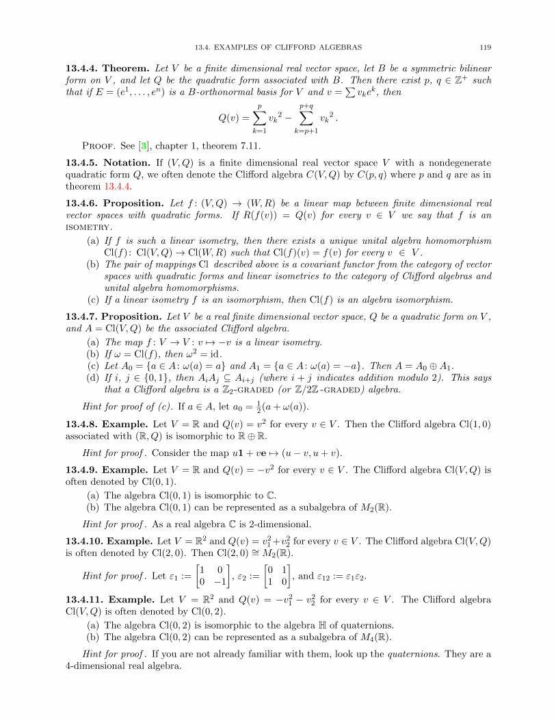
13.4. EXAMPLES OF CLIFFORD ALGEBRAS 119

13.4.4. Theorem. Let V be a finite dimensional real vector space, let B be a symmetric bilinearform on V , and let Q be the quadratic form associated with B. Then there exist p, q ∈ Z+ suchthat if E = (e1, . . . , en) is a B-orthonormal basis for V and v =

∑vke

k, then

Q(v) =

p∑k=1

vk2 −

p+q∑k=p+1

vk2 .

Proof. See [3], chapter 1, theorem 7.11.

13.4.5. Notation. If (V,Q) is a finite dimensional real vector space V with a nondegeneratequadratic form Q, we often denote the Clifford algebra C(V,Q) by C(p, q) where p and q are as intheorem 13.4.4.

13.4.6. Proposition. Let f : (V,Q) → (W,R) be a linear map between finite dimensional realvector spaces with quadratic forms. If R(f(v)) = Q(v) for every v ∈ V we say that f is anisometry.

(a) If f is such a linear isometry, then there exists a unique unital algebra homomorphismCl(f) : Cl(V,Q)→ Cl(W,R) such that Cl(f)(v) = f(v) for every v ∈ V .

(b) The pair of mappings Cl described above is a covariant functor from the category of vectorspaces with quadratic forms and linear isometries to the category of Clifford algebras andunital algebra homomorphisms.

(c) If a linear isometry f is an isomorphism, then Cl(f) is an algebra isomorphism.

13.4.7. Proposition. Let V be a real finite dimensional vector space, Q be a quadratic form on V ,and A = Cl(V,Q) be the associated Clifford algebra.

(a) The map f : V → V : v 7→ −v is a linear isometry.(b) If ω = Cl(f), then ω2 = id.(c) Let A0 = {a ∈ A : ω(a) = a} and A1 = {a ∈ A : ω(a) = −a}. Then A = A0 ⊕A1.(d) If i, j ∈ {0, 1}, then AiAj ⊆ Ai+j (where i + j indicates addition modulo 2). This says

that a Clifford algebra is a Z2-graded (or Z/2Z -graded) algebra.

Hint for proof of (c). If a ∈ A, let a0 = 12(a+ ω(a)).

13.4.8. Example. Let V = R and Q(v) = v2 for every v ∈ V . Then the Clifford algebra Cl(1, 0)associated with (R, Q) is isomorphic to R⊕ R.

Hint for proof . Consider the map u1 + ve 7→ (u− v, u+ v).

13.4.9. Example. Let V = R and Q(v) = −v2 for every v ∈ V . The Clifford algebra Cl(V,Q) isoften denoted by Cl(0, 1).

(a) The algebra Cl(0, 1) is isomorphic to C.(b) The algebra Cl(0, 1) can be represented as a subalgebra of M2(R).

Hint for proof . As a real algebra C is 2-dimensional.

13.4.10. Example. Let V = R2 and Q(v) = v21 +v2

2 for every v ∈ V . The Clifford algebra Cl(V,Q)is often denoted by Cl(2, 0). Then Cl(2, 0) ∼= M2(R).

Hint for proof . Let ε1 :=

[1 00 −1

], ε2 :=

[0 11 0

], and ε12 := ε1ε2.

13.4.11. Example. Let V = R2 and Q(v) = −v21 − v2

2 for every v ∈ V . The Clifford algebraCl(V,Q) is often denoted by Cl(0, 2).

(a) The algebra Cl(0, 2) is isomorphic to the algebra H of quaternions.(b) The algebra Cl(0, 2) can be represented as a subalgebra of M4(R).

Hint for proof . If you are not already familiar with them, look up the quaternions. They are a4-dimensional real algebra.

120 13. CLIFFORD ALGEBRAS

13.4.12. Exercise. Take a look at the web page [18] written by Pertti Lounesto.

13.4.13. Exercise. The Clifford algebra Cl(3, 1) (Minkowski space-time algebra) is isomorphic toM4(R).

Hint for proof . Exercise 13.4.12.

Bibliography

1. Ralph Abraham, Jerrold E. Marsden, and Tudor Ratiu, Manifolds, Tensor Analysis, and Applications, Addison-Wesley, Reading, MA, 1983. 112, 113, 114

2. Richard L. Bishop and Richard J. Crittenden, Geometry of Manifolds, Academic Press, New York, 1964. 81, 973. William C. Brown, A second Course in Linear Algebra, John Wiley, New York, 1988. 118, 1194. Stewart S. Cairns, A simple triangulation method for smooth manifolds, Bull. Amer. Math. Soc. 67 (1961),

389–390. 1085. P. M. Cohn, Basic Algebra: Groups, Rings and Fields, Springer, London, 2003. 76. J. Dieudonne, Treatise on Analysis, Volumes I and II, Academic Press, New York, 1969, 1970, [Di]. 657. Manfredo P. do Carmo, Differential Forms and Applications, Springer-Verlag, Berlin, 1994. 1148. John M. Erdman, A ProblemText in Advanced Calculus,

http://www.mth.pdx.edu/~erdman/PTAC/PTAClicensepage.html. 65, 84, 889. , A Companion to Real Analysis, 2007,

http://www.mth.pdx.edu/~erdman/CTRA/CRAlicensepage.html. 6510. Douglas R. Farenick, Algebras of Linear Transformations, Springer-Verlag, New York, 2001. 46, 4811. Kenneth Hoffman and Ray Kunze, Linear Algebra, second ed., Prentice Hall, Englewood Cliffs,N.J., 1971. 50, 6212. S. T. Hu, Differentiable Manifolds, Holt, Rinehart, and Winston, New York, 1969. 10813. Thomas W. Hungerford, Algebra, Springer-Verlag, New York, 1974. 714. Saunders Mac Lane and Garrett Birkhoff, Algebra, Macmillan, New York, 1967. 715. Serge Lang, Fundamentals of Differential Geometry, Springer Verlag, New York, 1999. 11316. John M. Lee, Introduction to Smooth Manifolds, Springer, New York, 2003. 81, 97, 10817. Lynn H. Loomis and Shlomo Sternberg, Advanced calculus, Jones and Bartlett, Boston, 1990. 6518. Pertti Lounesto, Counterexamples in Clifford Algebras, 1997/2002,

http://users.tkk.fi/~ppuska/mirror/Lounesto/counterexamples.htm. 12019. Ib Madsen and Jørgen Tornehave, From Calculus to Cohomology: de Rham cohomology and characteristic classes,

Cambridge University Press, Cambridge, 1997. 11320. Theodore W. Palmer, Banach Algebras and the General Theory of ∗-Algebras I–II, Cambridge University Press,

Cambridge, 1994/2001. 721. Charles C. Pinter, A Book of Abstract Algebra, second ed., McGraw-Hill, New York, 1990. 45, 7122. Steven Roman, Advanced Linear Algebra, second ed., Springer-Verlag, New York, 2005. 17, 62, 7423. I. M. Singer and J. A. Thorpe, Lecture Notes on Elementary Topology and Geometry, Springer Verlag, New York,

1967. 10824. Gerard Walschap, Metric Structures in Differential Geometry, Springer-Verlag, New York, 2004. 9725. Frank W. Warner, Foundations of Differentiable Manifolds and Lie Groups, Springer Verlag, New York, 1983.

108, 113

121

http://www.mth.pdx.edu/~erdman/PTAC/PTAClicensepage.html

http://www.mth.pdx.edu/~erdman/CTRA/CRAlicensepage.html

http://users.tkk.fi/~ppuska/mirror/Lounesto/counterexamples.htm

Index

α−1 (inverse of a morphism α), 28∧(V ) (Grassmann or exterior algebra), 77∧k(V ) (homogeneous elements of degree k), 77∇× ω (curl of a 1-form), 98∇f(m) (gradient of f at m), 98∇ · ω (divergence of a 1-form), 98∇φ(a) (gradient of φ at a), 68∂〈s〉 (boundary of a simplex), 107∂p (boundary map), 107χA

(characteristic function of A), 31f |A (restriction of f to A), 5∗ -algebra (algebra with involution), 58∗ -homomorphism (star homomorphism), 58

Sα // T (morphism in a category), 27

At (transpose of A), 17∧(M),

∧k(M) (differential forms), 96∧kF , 103〈x, v〉 (alternative notation for v∗(x)), 23f ∼ g (functions agree on some neighborhood), 87(f, g) (function into a product), 5S ⊗ T (tensor products of linear maps), 76⊕∞

k=0 Vk (direct sum), 32, 78BC (sums of products of elements in B and C), 38M ⊕N (inner product space direct sum of M

and N), 55M ⊕N (vector space direct sum of M and N), 12, 32U ⊗ V (tensor product), 74V/M (quotient of V by M), 32[x] ∧ [y] = [x⊗ y] in T (V )/J , 78ω ∧ µ (wedge product), 77f × g (product function), 5p g q (supremum of projections), 61p f q (infimum of projections), 61H N , 61M � V (M is a subspace of V ), 10V ∼= W (isomorphism of vector spaces), 21p � q (ordering of projections in a ∗ -algebra), 61p ⊥ q (orthogonality of projections), 61x ⊥ y (orthogonal vectors), 55[a, b] (closed segment in a vector space), 105|K| (polyhedron of a complex), 107A[x] (algebra of polynomials), 41A[[x]]

(algebra of formal power series), 41F[x] (polynomial algebra with coefficients in F), 41〈x, y〉 (inner product), 53βα (notation for composition of morphisms), 271 (standard one-element set), 6

T←(B) (inverse image of B under T ), 20T→(A) (direct image of A under T ), 20(s) = (v0, . . . , vp) (open p -simplex), 106[s] = [v0, . . . , vp] (closed p -simplex), 106〈s〉 = 〈v0, . . . , vp〉 (closed p -simplex), 106‖x‖ (norm of x), 54x (= Γ(x)), 24f ' g (f is tangent to g), 84' (tangency at 0), 66xs (alternative notation for x(s)), 7F⊥ (pre-annihilator of F ), 25

A⊥ (orthogonal complement of a set), 56

M⊥ (annihilator of M), 25T ∗ (inner product space adjoint of T ), 59T ∗ (vector space adjoint of T ), 29T t (transpose of T ), 59f←(B) (preimage of B under f), 29f→(A) (image of A under f), 29v∗, 23(V ∗, d), V ∗ (cochain complex), 104∂M (boundary of a manifold), 112∂Hn (boundary of a half-space), 112intM (interior of a manifold with boundary), 112intHn (interior of a half-space), 112[T ] (matrix representation of T ), 22[x] (equivalence class containing x), 32|A| (the forgetful functor acting on A), 29

0-form, 963-manifold, 812-manifold, 811-manifold, 81

Abelian group, 1AbGp

the category, 27absolutely

summablesequence, 11

additionpointwise, 3

additiveidentity, 1inverse, 1inverses, 8

adjoint, 59of the unilateral shift, 59vector space, 29

123

124 INDEX

adjointable, 59affine subspace, 106A(H,K), A(H) (adjointable maps), 59algebra, 38

Z+-graded, 77Clifford, 117commutative, 38de Rham cohomology, 104exterior, 77Grassmann, 77homomorphism, 38

unital, 38polynomial, 41quotient, 40simple, 39tensor, 78unital, 38

algebraictangent space, 87tangent vector, 87

algebraically closed, 44, 46ALG

bijective morphisms in, 38alternating, 72Altk(V ) (set of alternating k-linear maps), 78annihilating polynomial, 43annihilator, 7, 25antisymmetric, 15arithmetic

progression, 11associative, 8associativity, 1atlas, 82

smooth, 82atlases

compatible, 82equivalent, 82

basis, 14curves at a point, 85dual, 24for the geometric tangent space, 89ordered, 80orthonormal, 56right-handed, 80standard

for R3, 14for Rn, 14

βp (Betti number), 108Betti number, 103, 108bijection, 4bijective, 4bijective morphisms

are invertiblein ALG, 38

need not be invertiblein POSET, 28

bilinear, 71form

associated with a quadratic form, 117nondegenerate, 118

binary operation, 1ω × µ (cross-product of 1-forms), 98

Bk(M) (exact k-forms), 103B-orthonormal, 118bound

lower, 15upper, 15

boundaries, 107boundary

maps, 107of a half-space, 112of a manifold, 112of a simplex, 107

boundedfunction, 11sequence, 11B(S)

as a unital algebra, 39Bp(K) (space of simplicial p -coboundaries), 108Bp(K) (space of simplicial p -boundaries), 107bundle

cotangent, 96tangent, 95

C (set of complex numbers), 2C([a, b]) (continuous real valued functions), 19C1([a, b]) (continuously differentiable functions), 20calculus

polynomial functional, 42cancellable

left, 28right, 28

cancellation property, 7category, 27

AbGp as a, 27POSET as a, 27SET as a, 27VEC as a, 27concrete, 27

Cayley-Hamilton theorem, 48centered at, 82chain, 16chain rule, 87, 90, 92chains, 107change of variables, 89characteristic

Euler, 108polynomial, 47zero, 72

characteristic function, 31chart, 82charts

compatible, 82χ(K) (Euler characteristic), 108C∞ (smooth), 82

-manifold, 82C∞(M) (smooth real valued functions on M), 95C∞(U,Rn), 82

C∞(M,∧

(M)), C∞

(M,∧k(M)

)(smooth differential

forms), 97

INDEX 125

C∞m (M,R) (smooth functions defined in aneighborhood of m), 87

Cliffordalgebra, 117map, 117

closedalgebraically, 46differential form, 99face of a simplex, 106segment, 105simplex, 106

Cl(V,Q) (Clifford algebra), 117cm (tangency class of curves), 85coboundaries, 103coboundaryk-, 104operator, 104simplicial, 108

cochain, 108k-, 104complex, 104map, 105

cocyclek-, 104simplicial, 108

cocycles, 103codimension, 36codomain, 4coefficient

Fourier, 56leading, 42

cohomologyde Rham, 104group, 104

simplicial, 108cohomology group

de Rham, 103cokernel, 35cokerT (the cokernel of T ), 35column vector, 16combination

convex, 105formal linear, 31linear, 13

commutative, 8algebra, 38diagram, 4ring, 1

commutativity, 1comparable, 16compatible

atlases, 82charts, 82

complement, 12orthogonal, 56

complementary subspace, 12complete

order, 29complex

cochain, 104

simplicial, 106dimension of a, 107

vector space, 8components, 5composite, 81composition

of morphisms, 27concrete category, 27conjugate

linear, 53connecting maps, 81constant

locally, 103polynomial, 42

continuousdifferentiability, 20

continuously differentiable, 34contravariant, 28conventionsBC denotes sums of products of elements in B

and C, 38∧0(V ) = F, 78additive notation for Abelian groups, 3all k-forms are smooth differential k-forms, 97all categories are concrete, 27all charts belong to the differential structure, 82all differential forms are smooth, 97all manifolds are smooth, 82all one-forms are smooth differential one-forms, 96all unital rings are nontrivial, 2convolution a ∗ b written as a product ab, 41

dFm = dFm = dFm, 92for homomorphisms write gf for g ◦ f , 4for linear maps write TS for T ◦ S, 19for multiplication write xy for x · y, 1ideals are two-sided, 39identification of R with 1-dimensional tangent

spaces, 93identification of a vector with a scalar valued

function, 23in chapter 5 all vector spaces are real or complex,

53in chapters 10–11 all manifolds are smooth and

oriented, 95in chapters 10–11 all vector spaces are real, finite

dimensional, and oriented, 95in inner product spaces ”projection” means

”orthogonal projection”, 60in section 7.3 all fields are of characteristic zero, 72notation for composition

of algebra homomorphisms, 39of morphisms, 27

notations associated with 1-dimensional tangentspaces, 93

notations for a vector in a finite dimensional space,16

on Cartesian products, 5on ordering B-orthonormal bases, 118open subsets of Rn are manifolds in a canonical

fashion, 82

126 INDEX

spectrum of elements of nonunital algebras, 40the geometric and algebraic tangent spaces are

“the same”, 91when f is a 0-form, fω means f ∧ ω, 97write Tx for T (x) when T is linear, 19

convergentsequence, 11

convexcombination, 105hull, 106independent, 106set, 106

convolution, 41coordinate

projection, 82coordinate chart, 82coordinates, local, 82coproduct

in a category, 31uniqueness of, 32

cotangentbundle, 96

projection, 96cotangent space, 93covariant, 28Cp(K) (p -chains), 107

Cφ (map from Tm to Rn), 85Cp(K) (p -cochains), 108cross-product, 98curl, 98curve, 81, 84

at a point, 84parametrization of a, 81smooth, 81standard basis, 85

cycle, 71length of a, 71

cycles, 107

de Rham cohomology algebra, 104de Rham cohomology group, 103decomposable

element of a Grassmann algebra, 77tensor, 74

decompositiondiagonalizable plus nilpotent, 50primary, 50

decreasingsequence, 11

deg p (degree of a polynomial), 42degree

of a decomposable element, 77of a homogeneous element, 77of a polynomial, 42

∆fa (a translate of f), 66δ (diagonal mapping), 6dependent, 13derivation, 87derivative

directional, 68determinant, 73

function, 73

dFm (differential of f at m), 92

dFm (differential of f at m), 86diagonal

mapping, 6matrix, 49

diag(α1, . . . , αn) (diagonal matrix), 49diagonalizable, 49

plus nilpotent decomposition, 50unitarily, 62

diagramcommutative, 4

differentiable, 67continuously, 20, 34infinitely, 82

differential, 67k-form, 96form, 96

closed, 99exact, 99pullback of, 108smooth, 97

Gateaux, 68manifold, 82of a smooth map between manifolds, 86, 92one-form, 96structure, 82

dfa (the differential of f at a), 67differentiation

exterior, 97is linear, 20

dimensionof a simplex, 106of a simplicial complex, 107of a vector space, 17

dimK (dimension of a simplicial complex K), 107dimV (dimension of a vector space V ), 17direct

sumexternal, 78

direct image, 20direct sum

as a coproduct, 32as a product, 32external, 32external orthogonal, 55internal

for vector spaces, 12internal orthogonal, 55projections associated with, 47

directed segment, 3directional derivative, 68disjoint

permutations, 71distributivity, 1divergence, 98divω (divergence of a 1-form), 98divides, 43division

ring, 1

INDEX 127

division algorithm, 44divisor

greatest common, 45of zero, 7

domain, 4dom f (domain of a function f), 4dual basis, 24dual space, 23duality functor

for vector spaces, 29Dvf (directional derivative), 68

eigenspace, 48eigenspaces

generalized, 50eigenvalue, 47eigenvector, 48elementary tensor, 74ENM

(projection along N onto M), 37epic, 28epimorphism, 27εS , ε (function from S into 1), 6equivalent

atlases, 82orderings of vertices, 106unitarily, 62

essentialuniqueness, 32

Euclideanlocally, 82

Euler characteristic, 108even

permutation, 71even function, 12eventually

zero, 11exact

differential form, 99exact sequence

of cochain complexes, 105of vector spaces, 33short, 33

extension, 5exterior

algebra, 77differentiation operator, 97product, 77

externaldirect sum, 32, 55, 78

f (germ containing f), 87F(S)

as a commutative unital algebra, 38F(S), F(S,F), FS (F-valued functions on S), 7F(S,F), F(S)

F-valued functions on S, 3as a vector space, 9as an Abelian group, 3F(S, T ) (functions from S to T ), 7face, 106factorization, 45

field, 1algebraically closed, 44scalar, 68vector, 95

finitesupport, 7

finite dimensional, 17first isomorphism theorem, 33flat, 81forgetful functor, 28form

closed , 99differential, 96exact, 99multilinear, 71one-, 96quadratic, 117smooth differential, 97

formal linear combination, 31formal power series, 41Fourier

coefficient, 56sum, 56

Fψφ, Fφ (local representatives), 83free

object, 30vector space, 30

functionbounded, 11characteristic, 31diagonal, 6integrable, 11interchange, 6product, 5switching, 6

functionalcalculus

polynomial, 42linear, 23multilinear, 71Fa(V,W )

functions in a neighborhood of a, 65functor

contravariant, 28covariant, 28forgetful, 28power set, 29vector space duality, 29

fundamental quotient theorem, 33

Gateauxdifferential, 68variation, 68

Γ (the map from V to V ∗∗ taking x to x), 24generalized eigenspaces, 50geometic

progression, 11geometric

tangent space, 85tangent vector, 85

germs, 87

128 INDEX

Gm(M) (germs of functions at m), 87graded algebra, 77gradient, 98

at a point, 68on an open set, 68

grad f(m) (gradient of f at m), 98graph, 4Grassmann algebra, 77greatest common divisor, 45group, 1

Abelian, 1cohomology, 104de Rham cohomology, 103simplicial cohomology, 108simplicial homology, 107symmetric, 71

H(A) (self-adjoint elements of A), 58half-space

boundary of a, 112interior of a, 112

half-space, upper, 112Hermitian, 58Hk(M) (de Rham cohomology group), 103Hn (upper half-space), 112Hodge star operator, 80Hom(G,H)

as an Abelian group, 4Hom(G,H), Hom(G) (group homomorphisms), 4homogeneous

elements of a graded algebra, 77tensor, 74

homology, 107homomorphism

of Abelian groups, 4of algebras, 38

unital, 38of rings, 8unital ring, 8

Hp(K) (the pth simplicial cohomology group), 108

Hp(K) (the pth simplicial homology group), 107hull, convex, 106

idealin an algebra, 39left, 39principal, 39proper, 39right, 39trivial, 39

idempotent, 37, 41IV (identity operator on a vector space), 21idS (identity function on S), 5identity

additive, 1, 8function on a set, 5multiplicative, 1operator on a vector space, 21resolution of the, 47

image, 20, 29direct, 20

inverse, 20imaginary

part of a ∗ -algebra element, 59independent, 13

convex, 106indeterminant, 41inequality

Schwarz, 54infimum

of projections in a ∗ -algebra, 61infinite dimensional, 17infinitely differentiable, 82injection, 4injective, 4inner product, 53

space, 53spectral theorem for, 62

integrablefunction, 11

integralof a p -form over a p -chain, 111

integrationis linear, 19

interchange operation, 6interior

of a half-space, 112of a manifold with boundary, 112

internalorthogonal direct sum, 55

interpolationLagrange, 44

invariant subspace, 45trivial, 45

inverseadditive, 1, 8image, 20left, 28multiplicative, 1of a morphism, 28right, 28

invertible, 28element of an algebra, 39left, 21linear map, 21right, 21

involution, 58irreducible, 44isometry, 119isomorphic, 8, 38isomorphism, 21

in a category, 28of algebras, 38of rings, 8

k -coboundary, 104k -cochain, 104k -cocycle, 104kernel, 20

of a bilinear form, 118of a ring homomorphism, 8of an algebra homomorphism, 38

INDEX 129

kerT (the kernel of T ), 20k-form, 96

smooth, 97

l(S,F), l(S) (F-valued functions on S), 7l2(R), l2(C) (square summable sequences), 54Lagrange interpolation formula, 44largest, 15LatT , LatT (collection of invariant subspaces), 46lc(S,F), lc(S) (functions on S with finite support), 7lc(S,A) (functions from S into A with finite

support), 41leading coefficient, 42left

-handed basis, 80cancellable, 28ideal, 39inverse

of a morphism, 28invertible linear map, 21

Leibniz’s rule, 87length

of a cycle, 71of a vector, 54

linear, 19combination, 13

formal, 31trivial, 13

conjugate, 53functional, 23ordering, 16sesqui-, 53transformation

invertible, 21transformations, 19

tensor products of, 76L(V )

as a unital ∗ -algebra, 60as a unital algebra, 38

L(V,W ), L(V ) (family of linear functions), 19Ln(V1, . . . , Vn) (family of n-linear functions), 71linearly

dependent, 13independent, 13

linearly ordered set, 16local

coordinates, 82representative, 83

locallyEuclidean, 82smooth k-form, 97

locally constant, 103lower

bound, 15l(S,A) (functions from S into A), 41

manifold, 81boundary of a, 112differential, 82smooth, 82smoothly triangulated, 108

topological, 82with boundary, 112

interior of a, 112mapping

universal, 30matrix

diagonal, 49representation of an linear map, 22similarity, 48symmetric, 17transpose of a, 17

Mn

as a unital algebra, 39maximal, 15minimal, 15

polynomial, 43existence of, 43

Mm×n(F)as a vector space, 9

Mn(A) (n× n matrices of members of A), 72monic, 28monic polynomial, 42monoid, 1monomorphism, 27morphism

map, 28Mor(S, T ) (morphisms from S to T ), 27morphisms, 27

composition of, 27mT

(minimal polynomial for T ), 43multilinear, 71

form, 71functional, 71

multiplicationpointwise, 38

multiplicativeidentity, 1inverse, 1

N (set of natural numbers), 2N (A) (normal elements of A), 58nilpotent, 49n-linear function, 71n-manifold, 82Nn (first n natural numbers), 2nondegenerate bilinear form, 118norm, 54

uniform, 55normal, 58normalizing a vector, 56normed

linear space, 54vector space, see normed linear space

nullity, 20nullspace, 20numbers

special sets of, 2

objectfree, 30map, 28

130 INDEX

objects, 27odd

permutation, 71odd function, 12O(V,W ) (“big-oh” functions), 65o(V,W ) (“little-oh” functions), 65, 84ω(v) (a one-form acting on a vector field), 96one-form

differential, 96one-to-one, 4one-to-one correspondence, 4onto, 4open

face of a simplex, 106simplex, 106unit disc, 2

operationbinary, 1

operator, 19diagonalizable, 49exterior differentiation, 97nilpotent, 49projection, 37similarity, 48

opposite orientation, 80order

complete, 29preserving, 27

orderedbasis, 80by inclusion, 15partially, 15pointwise, 15

orderinglinear, 16partial

of projections, 61total, 16

orientationof a simplex, 106of a vector space, 80

orientedsimplex, 106vector space, 80

orthogonal, 55complement, 56direct sum

projections associated with, 62element of a real ∗ -algebra, 58inner product projections, 61projection, 60

associated with an orthogonal direct sumdecomposition, 62

projectionsin a ∗ -algebra, 61

resolution of the identity, 62with respect to a bilinear form, 118

orthonormal, 56basis, 56

orthonormal, B-, 118

overlap maps, 81

P(A) (projections on a ∗ -algebra), 60P(S) (power set of S), 29P(J) (polynomial functions on J), 14Pn(J) (polynomial functions of degree strictly less

than n), 14P2 (projective plane), 83parallelogram law, 54parametrization

of a curve, 81of a solid, 81of a surface, 81

partialordering, 15

of projections, 61p -boundaries, 107p -chains, 107p -coboundary

simplicial, 108p -cochain, 108p -cocycle

simplicial, 108p -cycles, 107permutation, 71

cyclic, 71even, 71odd, 71sign of a, 71

perpendicular, 55plane

of a simplex, 106Poincare’s lemma, 100point spectrum, 47pointwise

addition, 3multiplication, 38partial ordering, 15scalar multiplication, 9

polarization identity, 55polyhedron, 107polynomial, 41

algebra, 41annihilating, 43characteristic, 47constant, 42degree of a, 42function, 42functional calculus, 42irreducible, 44minimal, 43

existence of, 43monic, 42prime, 44reducible, 44standard form of a, 42

POSETbijective morphism in, 28the category, 28

POSETthe category, 27

INDEX 131

power seriesformal, 41

power set, 29functor, 29

(p, q)-shuffle, 79pre-annihilator, 25preimage, 29primary decomposition theorem, 50prime

relatively, 45prime polynomial, 44principal ideal, 39product

exterior, 77in a category, 31inner, 53tensor, 74uniqueness of, 32wedge, 77

progressionarithmetic, 11geometic, 11

projectionalong one subspace onto another, 37assocuated with direct sum decomposition, 47coordinate, 82cotangent bundle, 96in a ∗ -algebra, 60operator, 37orthogonal, 60, 61tangent bundle, 95

projectionsdifference of, 61infimum of, 61ordering of, 61orthogonality of, 61product of, 61sum of, 61supremum of, 61

projective plane, 83proper

ideal, 39p -simplex, 106pullback of differential forms, 108Pythagorean theorem, 55

Q (set of rational numbers), 2quadratic form, 117

associated with a bilinear form, 117quotient

algebra, 40map, 32, 33object, 32vector space, 33

quotient map, the, 40

R (set of real numbers), 2range, 20ranT (the range of T ), 20rank, 20rank-plus-nullity theorem, 33

realline

special subsets of, 2part of a ∗ -algebra element, 59vector space, 8

reducible, 44reducing subspaces, 45reflexive, 15relation, 15relatively prime, 45representation

matrix, 22representative, local, 83resolution of the identity

in vector spaces, 47orthogonal, 62

restriction, 5retraction, 21reverse orientation, 80ρM

(cotangent bundle projection), 96Riesz-Frechet theorem

for inner product spaces, 57for vector spaces, 24

right-handed basis, 80cancellable, 28ideal, 39inverse

of a morphism, 28invertible linear map, 21

R∞as a vector space, 9as an Abelian group, 3

ring, 1commutative, 1division, 1homomorphism, 8

unital, 8with identity, 1

Rnas a vector space, 9as an Abelian group, 3

Rn (set of n-tuples of real numbers), 2root, 45row vector, 16r -skeleton, 107

S1 (unit circle), 2S1 (unit circle), 82Sn (n-sphere), 83scalar, 8

field, 68multiplication

pointwise, 9Schwarz inequality, 54section, 21, 95segment, 3segment, closed, 105self-adjoint, 58semigroup, 1separates points, 23

132 INDEX

sequencebounded, 11convergent, 11decreasing, 11exact, 33

seriesformal power, 41

sesquilinear, 53SET

the category, 27shift

unilateral, 20short exact sequence, 33, 105shuffle, 79σ (interchange operation), 6σ(a), σA(a) (the spectrum of a), 40σp(A), σp(T ) (point spectrum), 47sign

of a permutation, 71similar, 48simple

algebra, 39simplex

closed, 106dimension of a, 106face of a, 106open, 106oriented, 106plane of a, 106vertex of a, 106

simplicialcoboundary, 108cocycle, 108cohomology group, 108complex, 106

dimension of a, 107simplicial homology group, 107skeleton of a complex, 107skew-Hermitian, 58skew-symmetric, 58, 72smallest, 15

subspace containing a set of vectors, 11smooth, 82k-form, 97atlas, 82curve, 81differential form, 97differential one-form, 96function, 81locally, 97manifold, 82map between manifolds, 83solid, 81submanifold, 108surface, 81triangulation, 108vector field, 95

smoothly compatibleatlases, 82charts, 82

solid, 81parametrization of a, 81smooth, 81

spacealgebraic tangent, 87geometric tangent, 85inner product, 53normed linear, 54vector, 8

span, 13of the empty set, 13

span(A) (the span of A), 13spectral theorem

for complex inner product spaces, 62for vector spaces, 49

spectrum, 40point, 47

S(p, q) (shuffle permutations), 79square summable sequence, 54standard basis

curves at a point, 85for Pn(J), 14for Mm×n, 15for R3, 14for Rn, 14

standard form of a polynomial, 42star operator, 80star-algebra, 58star-homomorphism, 58stereographic projection, 83Stokes’ theorem, 113structure

differential, 82subalgebra, 39

unital, 39submanifold, 108subprojection, 61subspace, 10

affine, 106complementary, 12invariant, 45reducing, 45

sumdirect, 32, 78Fourier, 56internal direct, 12

summableabsolutely, 11square, 54

supp(f) (support of f), 7support, 7

finite, 7supremum

of projections in a ∗ -algebra, 61surface, 81

parametrization of a, 81smooth, 81

surjection, 4surjective, 4switching operation, 6

INDEX 133

symmetricelement of a real ∗ -algebra, 58group, 71matrix, 17skew-, 72

tangentat 0, 84at m, 84bundle, 95

projection, 95space

algebraic, 87geometric, 85

vectoralgebraic, 87geometric, 85

tangent (at zero), 66τM

(tangent bundle projection), 95tensor

algebra, 78decomposable, 74elementary, 74homogeneous, 74product, 74

of linear maps, 76T -invariant subspace, 45TM (tangent bundle), 95T ∗M (cotangent bundle), 96Tm (tangent space at m), 91

Tm(M) (algebraic tangent space at m), 87

Tm(M) (geometric tangent space at m), 85topological

manifold, 82total

ordering, 16transition maps, 81transitive

algebra, 46propertty of a partial ordering, 15

transpose, 59, 73of a matrix, 17

transposition, 71triangulated manifold, 108trilinear, 71trivial

LatT or LatT, 46ideal, 39invariant subspaces, 45linear combination, 13vector space, 8T (V ) (the tensor algebra of V ), 78

U(A) (unitary elements of A), 58uniform

norm, 55unilateral shift, 20

is adjointable on l2, 59unique factorization theorem, 45uniqueness

essential, 32

of products, coproducts, 32unit, 1

vector, 54unital

algebra, 38algebra homomorphism, 38ring, 1ring homomorphism, 8subalgebra, 39

unitarilydiagonalizable, 62equivalent, 62

unitary, 58unitization, 40universal, 117

mappingdiagram, 30property, 30

upperbound, 15half-space, 112

V ∗ (dual space of V ), 23variation

Gateaux, 68vector, 8

algebraic tangent, 87column, 16field, 95geometric tangent, 85norm of a, 54row, 16space, 8

adjoint map, 29complex, 8dimension of a, 17free, 30normed, 54orientation of a, 80oriented, 80real, 8spectral theorem for, 49trivial, 8

unit, 54VEC

the category, 27vertex

of a simplex, 106vf (action of a vector field on a function), 95vol (volume element or form), 80volume

element, 80

wedge product, 77

Z (set of integers), 2zero

divisor, 7form, 96

Z+-graded algebra, 77Zk(M) (closed k-forms), 103

134 INDEX

Zorn’s lemma, 16Zp(K) (space of simplicial p -cocycles), 108Zp(K) (space of simplicial p -cycles), 107

multilinear algebra

Documents

differential manifolds

linear independence

tensor products of linear

study of linear

elements of linear

linear combinations

linear transformations

dual spaces