multiagent systems and distributed ai - citeseer
TRANSCRIPT

A Concise Introduction to
Multiagent Systems and
Distributed AI
Nikos Vlassis
Intelligent Autonomous SystemsInformatics Institute
University of Amsterdam
Universiteit van Amsterdam

c© 2003 Nikos Vlassis, University of Amsterdam

Contents
Preface iii
1 Introduction 1
1.1 Multiagent systems and distributed AI . . . . . . . . . . . . . 1
1.2 Characteristics of multiagent systems . . . . . . . . . . . . . . 1
1.3 Applications . . . . . . . . . . . . . . . . . . . . . . . . . . . . 4
1.4 Challenging issues . . . . . . . . . . . . . . . . . . . . . . . . 5
1.5 Notes and further reading . . . . . . . . . . . . . . . . . . . . 6
2 Rational agents 7
2.1 What is an agent? . . . . . . . . . . . . . . . . . . . . . . . . 7
2.2 Agents as rational decision makers . . . . . . . . . . . . . . . 8
2.3 Observable worlds and the Markov property . . . . . . . . . . 8
2.4 Stochastic transitions and utilities . . . . . . . . . . . . . . . 10
2.5 Notes and further reading . . . . . . . . . . . . . . . . . . . . 14
3 Strategic games 15
3.1 Game theory . . . . . . . . . . . . . . . . . . . . . . . . . . . 15
3.2 Strategic games . . . . . . . . . . . . . . . . . . . . . . . . . . 16
3.3 Iterated elimination of strictly dominated actions . . . . . . . 18
3.4 Nash equilibrium . . . . . . . . . . . . . . . . . . . . . . . . . 19
3.5 Notes and further reading . . . . . . . . . . . . . . . . . . . . 22
4 Coordination 23
4.1 Distributed decision making . . . . . . . . . . . . . . . . . . . 23
4.2 Coordination games . . . . . . . . . . . . . . . . . . . . . . . 24
4.3 Social conventions . . . . . . . . . . . . . . . . . . . . . . . . 25
4.4 Roles . . . . . . . . . . . . . . . . . . . . . . . . . . . . . . . . 26
4.5 Coordination graphs . . . . . . . . . . . . . . . . . . . . . . . 28
4.6 Notes and further reading . . . . . . . . . . . . . . . . . . . . 31
5 Common knowledge 33
5.1 Thinking interactively . . . . . . . . . . . . . . . . . . . . . . 33
5.2 The puzzle of the hats . . . . . . . . . . . . . . . . . . . . . . 34
i
5.3 Partial observability and information . . . . . . . . . . . . . . 345.4 A model of knowledge . . . . . . . . . . . . . . . . . . . . . . 375.5 Knowledge and actions . . . . . . . . . . . . . . . . . . . . . . 385.6 Notes and further reading . . . . . . . . . . . . . . . . . . . . 40
6 Communication 416.1 Communicating agents . . . . . . . . . . . . . . . . . . . . . . 416.2 Communicative acts . . . . . . . . . . . . . . . . . . . . . . . 426.3 The value of communication . . . . . . . . . . . . . . . . . . . 436.4 Coordination via communication . . . . . . . . . . . . . . . . 456.5 Notes and further reading . . . . . . . . . . . . . . . . . . . . 48
7 Mechanism design 497.1 Self-interested agents . . . . . . . . . . . . . . . . . . . . . . . 497.2 The mechanism design problem . . . . . . . . . . . . . . . . . 507.3 The revelation principle . . . . . . . . . . . . . . . . . . . . . 537.4 The Groves-Clarke mechanism . . . . . . . . . . . . . . . . . 547.5 Notes and further reading . . . . . . . . . . . . . . . . . . . . 55
8 Learning 578.1 Reinforcement learning . . . . . . . . . . . . . . . . . . . . . . 578.2 Markov decision processes . . . . . . . . . . . . . . . . . . . . 588.3 Multiagent reinforcement learning . . . . . . . . . . . . . . . 608.4 Exploration policies . . . . . . . . . . . . . . . . . . . . . . . 628.5 Notes and further reading . . . . . . . . . . . . . . . . . . . . 63

Preface
This text contains introductory material on the subject of Multiagent Sys-tems and Distributed AI. It has been used as lecture notes for 3rd and 4thyear courses at the Informatics Institute of the University of Amsterdam,The Netherlands. An on-line version can be found at
http://www.science.uva.nl/~vlassis/cimasdai/
with a link to accompanying software. I would be most grateful to receiveany kind of feedback on this text, concerning errors, ideas for improvement,etc. You may contact me at
I would like to thank the following people for providing useful comments onthe text: Taylan Cemgil, Jelle Kok, Jan Nunnink, Matthijs Spaan.
Nikos VlassisAmsterdam, September 2003
Version: 14 October 2003
iii

iv PREFACE

Chapter 1
Introduction
In this chapter we give a brief introduction to multiagent systems, discusstheir differences with single-agent systems, and outline possible applicationsand challenging issues for research.
1.1 Multiagent systems and distributed AI
The modern approach to artificial intelligence (AI) is centered aroundthe concept of a rational agent. An agent is anything that can perceiveits environment through sensors and act upon that environment throughactuators (Russell and Norvig, 2003). An agent that always tries to opti-mize an appropriate performance measure is called a rational agent. Such adefinition of a rational agent is fairly general and can include human agents(having eyes as sensors, hands as actuators), robotic agents (having cam-eras as sensors, wheels as actuators), or software agents (having a graphicaluser interface as sensor and as actuator). From this perspective, AI canbe regarded as the study of the principles and design of artificial rationalagents.
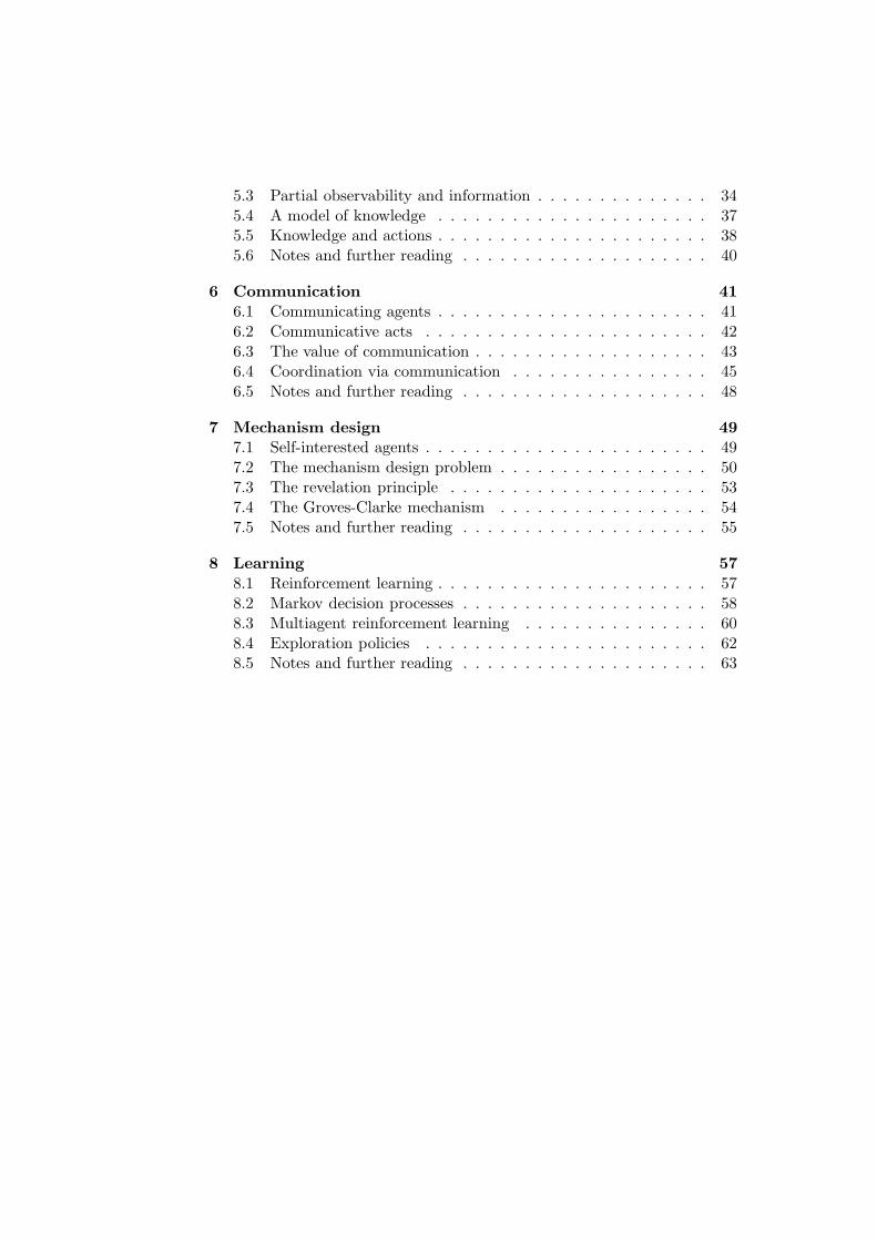
However, agents are seldom stand-alone systems. In many situationsthey coexist and interact with other agents in several different ways. Ex-amples include software agents on the Internet, soccer playing robots (seeFig. 1.1), and many more. Such a system that consists of a group of agentsthat can potentially interact with each other is called a multiagent system(MAS), and the corresponding subfield of AI that deals with principles anddesign of multiagent systems is called distributed AI.
1.2 Characteristics of multiagent systems
What are the fundamental aspects that characterize a MAS and distinguishit from a single-agent system? One can think along the following dimensions:
1
2 CHAPTER 1. INTRODUCTION
Figure 1.1: A robot soccer team is an example of a multiagent system.
Agent design
It is often the case that the various agents that comprise a MAS are designedin different ways. A typical example is software agents, also called softbots,that have been implemented by different people. In general, the design dif-ferences may involve the hardware (for example soccer robots based on dif-ferent mechanical platforms), or the software (for example software agentsrunning different operating systems). We often say that such agents are het-erogeneous in contrast to homogeneous agents that are designed in anidentical way and have a priori the same capabilities. However, this distinc-tion is not clear-cut; agents that are based on the same hardware/softwarebut implement different behaviors can also be called heterogeneous. Agentheterogeneity can affect all functional aspects of an agent from perceptionto decision making, while in single-agent systems the issue is simply nonex-istent.
Environment
Agents have to deal with environments that can be either static (time-invariant) or dynamic (nonstationary). Most existing AI techniques forsingle agents have been developed for static environments because these areeasier to handle and allow for a more rigorous mathematical treatment. Ina MAS, the mere presence of multiple agents makes the environment appeardynamic from the point of view of each agent. This can often be problematic,for instance in the case of concurrently learning agents where non-stablebehavior can be observed. There is also the issue which parts of a dynamicenvironment an agent should treat as other agents and which not. We willdiscuss some of these issues in chapter 8.

1.2. CHARACTERISTICS OF MULTIAGENT SYSTEMS 3
Perception
The collective information that reaches the sensors of the agents in a MASis typically distributed: the agents may observe data that differ spatially(appear at different locations), temporally (arrive at different times), or evensemantically (require different interpretations). This automatically makesthe world state partially observable to each agent, which has various con-sequences in the decision making of the agents. An additional issue is sensorfusion, that is, how the agents can optimally combine their perceptions inorder to increase their collective knowledge about the current state. We willdiscuss distributed perception and its consequences in chapter 5.
Control
Contrary to single-agent systems, the control in a MAS is typically dis-tributed (decentralized). This means that there is no central process thatcollects information from each agent and then decides what action each agentshould take. The decision making of each agent lies to a large extent withinthe agent itself. The general problem of multiagent decision making is thesubject of game theory which we will cover in chapter 3. In a cooperativeor team MAS1, distributed decision making results in asynchronous compu-tation and certain speedups, but it also has the downside that appropriatecoordination mechanisms need to be additionally developed. Coordina-tion ensures that the individual decisions of the agents result in good jointdecisions for the group. Chapter 4 is devoted to the topic of coordination.
Knowledge
In single-agent systems we typically assume that the agent knows its ownactions but not necessarily how the world is affected by its actions. In aMAS, the levels of knowledge of each agent about the current world statecan differ substantially. For example, in a team MAS involving two homo-geneous agents, each agent may know the available action set of the otheragent, both agents may know (by communication) their current perceptions,or they can infer the intentions of each other based on some shared priorknowledge. On the other hand, an agent that observes an adversarial teamof agents will typically be unaware of their action sets and their currentperceptions, and might also be unable to infer their plans. In general, in aMAS each agent must also consider the knowledge of each other agent in itsdecision making. A crucial concept here is that of common knowledge,according to which every agent knows a fact, every agent knows that every
1We will interchangeably use the terms ‘cooperative’ or ‘team’ MAS to refer to agentsthat share the same interests. We note, however, that the game-theoretic use of the term‘cooperative’ is different, referring to agents that are freely allowed to communicate andenforce agreements prior to taking decisions (Harsanyi and Selten, 1988).

4 CHAPTER 1. INTRODUCTION
other agent knows this fact, and so on. We will discuss common knowledgein detail in chapter 5.
Communication
Interaction is often associated with some form of communication. Typ-ically we view communication in a MAS as a two-way process, where allagents can potentially be senders and receivers of messages. Communica-tion can be used in several cases, for instance, for coordination among co-operative agents or for negotiation among self-interested agents (we willdiscuss the latter case in some detail in chapter 7). Moreover, communica-tion additionally raises the issues of what network protocols to use in orderfor the exchanged information to arrive safely and timely, and what lan-guage the agents must speak in order to understand each other (especiallyif they are heterogeneous). We will address communication in chapter 6.
1.3 Applications
Just as with single-agent systems in traditional AI, it is difficult to anticipatethe full range of applications where MASs can be used. Some applicationshave already appeared, especially in software engineering where MAS tech-nology is viewed as a novel and promising software building paradigm. Acomplex software system can be treated as a collection of many small-sizeautonomous agents, each with its own local functionality and properties, andwhere interaction among agents enforces total system integrity. Some of thebenefits of using MAS technology in large software systems are (Sycara,1998):
• Speedup and efficiency, due to the asynchronous and parallel compu-tation.
• Robustness and reliability, in the sense that the whole system canundergo a ‘graceful degradation’ when one or more agents fail.
• Scalability and flexibility, since it is easy to add new agents to thesystem.
• Cost, assuming that an agent is a low-cost unit compared to the wholesystem.
• Development and reusability, since it is easier to develop and maintaina modular software than a monolithic one.
A very challenging application domain for MAS technology is the Inter-net. Today the Internet has developed into a highly distributed open system

1.4. CHALLENGING ISSUES 5
where heterogeneous software agents come and go, there are no well estab-lished protocols or languages on the ‘agent level’ (higher than TCP/IP),and the structure of the network itself keeps on changing. In such an envi-ronment, MAS technology can be used to develop agents that act on behalfof a user and are able to negotiate with other agents in order to achievetheir goals. Auctions on the Internet and electronic commerce are such ex-amples (Noriega and Sierra, 1999; Sandholm, 1999). One can also thinkof applications where agents can be used for distributed data mining andinformation retrieval.
MASs can also be used for traffic control where agents (software orrobotic) are located in different locations, receive sensor data that are geo-graphically distributed, and must coordinate their actions in order to ensureglobal system optimality (Lesser and Erman, 1980). Other applications arein social sciences where MAS technology can be used for simulating inter-activity and other social phenomena (Gilbert and Doran, 1994), in roboticswhere a frequently encountered problem is how a group of robots can lo-calize themselves within their environment (Roumeliotis and Bekey, 2002),and in virtual reality and computer games where the challenge is to buildagents that exhibit intelligent behavior (Terzopoulos, 1999).
Finally, an application of MASs that has recently gained popularity isrobot soccer. There, teams of real or simulated autonomous robots playsoccer against each other (Kitano et al., 1997). Robot soccer provides atestbed where MAS algorithms can be tested, and where many real-worldcharacteristics are present: the domain is continuous and dynamic, the be-havior of the opponents may be difficult to predict, there is uncertainty inthe sensor signals, etc.
1.4 Challenging issues
The transition from single-agent systems to MASs offers many potentialadvantages but also raises challenging issues. Some of these are:
• How to decompose a problem, allocate subtasks to agents, and syn-thesize partial results.
• How to handle the distributed perceptual information. How to enableagents to maintain consistent shared models of the world.
• How to implement decentralized control and build efficient coordina-tion mechanisms among agents.
• How to design efficient multiagent planning and learning algorithms.
• How to represent knowledge. How to enable agents to reason aboutthe actions, plans, and knowledge of other agents.
6 CHAPTER 1. INTRODUCTION
• How to enable agents to communicate. What communication lan-guages and protocols to use. What, when, and with whom should anagent communicate.
• How to enable agents to negotiate and resolve conflicts.
• How to enable agents to form organizational structures like teams orcoalitions. How to assign roles to agents.
• How to ensure coherent and stable system behavior.
Clearly the above problems are interdependent and their solutions mayaffect each other. For example, a distributed planning algorithm may re-quire a particular coordination mechanism, learning can be guided by theorganizational structure of the agents, and so on. In the following chapterswe will try to provide answers to some of the above questions.
1.5 Notes and further reading
The review articles of Sycara (1998) and Stone and Veloso (2000) provideconcise and readable introductions to the field. The textbooks of Huhns(1987), Singh (1994), O’Hare and Jennings (1996), Ferber (1999), Weiss(1999), and Wooldridge (2002) offer more extensive treatments, emphasizingdifferent AI and software engineering aspects. A website on multiagentsystems is: www.multiagent.com

Chapter 2
Rational agents
In this chapter we describe what a rational agent is, we investigate somecharacteristics of an agent’s environment like observability and the Markovproperty, and we examine what is needed for an agent to behave optimallyin an uncertain world where actions do not always have the desired effects.
2.1 What is an agent?
Following Russell and Norvig (2003), an agent is anything that can beviewed as perceiving its environment through sensors and acting uponthat environment through actuators.1 Examples include humans, robots, orsoftware agents. We often use the term autonomous to refer to an agentwhose decision making relies to a larger extent on its own perception thanto prior knowledge given to it at design time.
In this chapter we will study the problem of optimal decision makingof an agent. That is, how an agent can choose the best possible action ateach time step, given what it knows about the world around it. We will saythat an agent is rational if it always selects an action that optimizes anappropriate performance measure, given what the agent knows so far.The performance measure is typically defined by the user (the designer ofthe agent) and reflects what the user expects from the agent in the task athand. For example, a soccer robot must act so as to maximize the chanceof scoring for its team, a software agent in an electronic auction must tryto minimize expenses for its designer, and so on. A rational agent is alsocalled an intelligent agent.
In the following we will mainly focus on computational agents, thatis, agents that are explicitly designed for solving a particular task and areimplemented on some computing device.
1In this chapter we will use ‘it’ to refer to an agent, to emphasize that we are talkingabout computational entities.
7

8 CHAPTER 2. RATIONAL AGENTS
2.2 Agents as rational decision makers
The problem of optimal decision making of an agent was first studied inoptimal control (Bellman, 1961). For the purpose of our discussion, wewill assume a discrete set of time steps t = 1, 2, . . ., in each of which theagent must choose an action at from a finite set of actions A that it hasavailable. Intuitively, in order to act rationally, an agent should take boththe past and the future into account when choosing an action. The pastrefers to what the agent has perceived and what actions it has taken untiltime t, and the future refers to what the agent expects to perceive and doafter time t.
If we denote by oτ the perception of an agent at time τ , then the aboveimplies that in order for an agent to optimally choose an action at time t, itmust in general use its complete history of perceptions oτ and actions aτ
for τ ≤ t. The function
π(o1, a1, o2, a2, . . . , ot) = at (2.1)
that in principle would require mapping the complete history of perception-action pairs up to time t to an optimal action at is called the policy of theagent.
As long as we can find a function π that implements the above mapping,the part of optimal decision making that refers to the past is solved. How-ever, defining and implementing such a function is problematic; the completehistory can consist of a very large (even infinite) number of perception-action pairs, which can vary from one task to another. Merely storing allperceptions would require very large memory, aside from the computationalcomplexity for actually computing π.
This fact calls for simpler policies. One possibility is for the agent toignore all its percept history except for the last perception ot. In this caseits policy takes the form
π(ot) = at (2.2)
which is a mapping from the current perception of the agent to an action.An agent that simply maps its current perception ot to a new action at, thuseffectively ignoring the past, is called a reflex agent, and its policy (2.2) iscalled reactive or memoryless. A natural question to ask now is: howsuccessful such a reflex agent can be? As we will see next, for a particularclass of environments a reflex agent can do pretty well.
2.3 Observable worlds and the Markov property
From the discussion above it is clear that the terms ‘agent’ and ‘environment’are coupled, so that one cannot be defined without the other. In fact, thedistinction between an agent and its environment is not always clear, and it

2.3. OBSERVABLE WORLDS AND THE MARKOV PROPERTY 9
is sometimes difficult to draw a line between these two (Sutton and Barto,1998, ch. 3).
To simplify things we will assume hereafter the existence of a world inwhich one or more agents are embedded, and in which they perceive, think,and act. The collective information that is contained in the world at anytime step t, and that is relevant for the task at hand, will be called a stateof the world and denoted by st. The set of all states of the world will bedenoted by S. As an example, in a robot soccer game a world state can becharacterized by the the soccer field layout, the positions and velocities ofall players and the ball, what each agent knows about each other, and otherparameters that are relevant to the decision making of the agents like theelapsed time since the game started, etc.
Depending on the nature of problem, a world can be either discreteor continuous. A discrete world can be characterized by a finite numberof states. Examples are the possible board configurations in a chess game.On the other hand, a continuous world can have infinitely many states. Forexample, for a mobile robot that translates and rotates freely in a staticenvironment and has coordinates (x, y, θ) with respect to a fixed Cartesianframe holds S = IR3. Most of the existing AI techniques have been developedfor discrete worlds, and this will be our main focus as well.
Observability
A fundamental property that characterizes a world from the point of view ofan agent is related to the perception of the agent. We will say that the worldis (fully) observable to an agent if the current perception ot of the agentcompletely reveals the current state of the world, that is, st = ot. On theother hand, in a partially observable world the current perception ot ofthe agent provides only partial information about the current world state inthe form of a conditional probability distribution P (st|ot) over states. Thismeans that the current perception ot does not fully reveal the true worldstate, but to each state st the agent assigns probability P (st|ot) that st isthe true state (with 0 ≤ P (st|ot) ≤ 1 and
∑
st∈S P (st|ot) = 1). Here wetreat st as a random variable that can take all possible values in S.
Partial observability can in principle be attributed to two factors. First,it can be the result of noise in the agent’s sensors. For example, due tosensor malfunction, the same state may ‘generate’ different perceptions tothe agent at different points in time. That is, every time the agent visits aparticular state it may perceive something different. Second, partial observ-ability can be related to an inherent property of the environment referred toas perceptual aliasing: different states may produce identical perceptionsto the agent at different time steps. In other words, two states may ‘look’the same to an agent, although the states are different from each other. Forexample, two identical doors along a corridor will look exactly the same to

10 CHAPTER 2. RATIONAL AGENTS
the eyes of a human or the camera of a mobile robot, no matter how accurateeach sensor system is.
Partial observability is much harder to handle than full observability, andalgorithms for optimal sequential decision making in a partially observableworld can easily become intractable (Russell and Norvig, 2003, sec. 17.4).Partial observability is of major concern especially in multiagent systemswhere, as it will also be clearer in chapter 5, it may affect not only what eachagent knows about the world state, but also what each agent knows abouteach other’s knowledge. We will defer partial observability until chapter 5.
The Markov property
Let us consider again the case of a reflex agent with a reactive policy π(ot) =at in a fully observable world. The assumption of observability impliesst = ot, and therefore the policy of the agent reads
π(st) = at. (2.3)
In other words, in an observable world the policy of a reflex agent is amapping from world states to actions. The gain comes from the fact thatin many problems the state of the world at time t provides a completedescription of the history before time t. Such a world state that summarizesall the relevant information about the past in a particular task is said to beMarkov or to have the Markov property. As we conclude from the above,in a Markov world an agent can safely use the memoryless policy (2.3) for itsdecision making, in place of the theoretically optimal policy function (2.1)that in principle would require very large memory.
So far we have discussed how the policy of an agent may depend onits past experience and the particular characteristics of the environment.However, as we argued at the beginning, optimal decision making shouldalso take the future into account. This is what we are going to examinenext.
2.4 Stochastic transitions and utilities
As mentioned above, at each time step t the agent chooses an action at froma finite set of actions A. When the agent takes an action, the world changesas a result of this action. A transition model (sometimes also called worldmodel) specifies how the world changes when an action is executed. If thecurrent world state is st and the agent takes action at, we can distinguishthe following two cases:
• In a deterministic world, the transition model maps a state-actionpair (st, at) to a single new state st+1. In chess for example, every movechanges the configuration on the board in a deterministic manner.

2.4. STOCHASTIC TRANSITIONS AND UTILITIES 11
• In a stochastic world, the transition model maps a state-action pair(st, at) to a probability distribution P (st+1|st, at) over states. As inthe partial observability case above, st+1 is a random variable thatcan take all possible values in S, each with corresponding probabilityP (st+1|st, at). Most real-world applications involve stochastic transi-tion models, for example, robot motion is inaccurate because of wheelslip and other effects.
We saw in the previous section that sometimes partial observability canbe attributed to uncertainty in the perception of the agent. Here we seeanother example where uncertainty plays a role; namely, in the way theworld changes when the agent executes an action. In a stochastic world,the effects of the actions of the agent are not known a priori. Instead,there is a random element that decides how the world changes as a resultof an action. Clearly, stochasticity in the state transitions introduces anadditional difficulty in the optimal decision making task of the agent.
From goals to utilities
In classical AI, a goal for a particular task is a desired state of the world.Accordingly, planning is defined as a search through the state space for anoptimal path to the goal. When the world is deterministic, planning comesdown to a graph search problem for which a variety of methods exist, seefor example (Russell and Norvig, 2003, ch. 3).
In a stochastic world, however, planning can not be done by simplegraph search because transitions between states are nondeterministic. Theagent must now take the uncertainty of the transitions into account whenplanning. To see how this can be realized, note that in a deterministic worldan agent prefers by default a goal state to a non-goal state. More generally,an agent may hold preferences between any world states. For example, asoccer agent will mostly prefer to score, will prefer less (but still a lot) tostand with the ball in front of an empty goal, and so on.
A way to formalize the notion of state preferences is by assigning toeach state s a real number U(s) that is called the utility of state s for thatparticular agent. Formally, for two states s and s′ holds U(s) > U(s′) if andonly if the agent prefers state s to state s′, and U(s) = U(s′) if and only ifthe agent is indifferent between s and s′. Intuitively, the utility of a stateexpresses the ‘desirability’ of that state for the particular agent; the largerthe utility of the state, the better the state is for that agent. In the worldof Fig. 2.1, for instance, an agent would prefer state d3 than state b2 or d2.Note that in a multiagent system, a state may be desirable to a particularagent and at the same time be undesirable to an other agent; in soccer, forexample, scoring is typically unpleasant to the opponent agents.

12 CHAPTER 2. RATIONAL AGENTS
4
3 +1
2 −1 −1
1 start
a b c d
Figure 2.1: A world with one desired (+1) and two undesired (−1) states.
Decision making in a stochastic world
Equipped with utilities, the question now is how an agent can efficiently usethem for its decision making. Let us assume that the world is stochasticwith transition model P (st+1|st, at), and is currently in state st, while anagent is pondering how to choose its action at. Let U(s) be the utilityof state s for the particular agent (we assume there is only one agent inthe world). Utility-based decision making is based on the premise that theoptimal action a∗
t of the agent should maximize expected utility, that is,
a∗t = arg maxat∈A
∑
st+1
P (st+1|st, at)U(st+1) (2.4)
where we sum over all possible states st+1 ∈ S the world may transition to,given that the current state is st and the agent takes action at. In words,to see how good an action is, the agent has to multiply the utility of eachpossible resulting state with the probability of actually reaching this state,and sum up the resulting terms. Then the agent must choose the action a∗
t
that gives the highest sum.
If each world state has a utility value, then the agent can do the abovecalculations and compute an optimal action for each possible state. Thisprovides the agent with a policy that maps states to actions in an optimalsense. In particular, given a set of optimal (i.e., highest attainable) utilitiesU∗(s) in a given task, the greedy policy
π∗(s) = arg maxa
∑
s′
P (s′|s, a)U ∗(s′) (2.5)
is an optimal policy for the agent.
There is an alternative and often useful way to characterize an optimalpolicy. For each state s and each possible action a we can define an optimalaction value (or Q-value) Q∗(s, a) that measures the ‘goodness’ of action ain state s for that agent. For this value holds U ∗(s) = maxa Q∗(s, a), whilean optimal policy can be computed as
π∗(s) = arg maxa
Q∗(s, a) (2.6)

2.4. STOCHASTIC TRANSITIONS AND UTILITIES 13
4 0.818 (→) 0.865 (→) 0.911 (→) 0.953 (↓)
3 0.782 (↑) 0.827 (↑) 0.907 (→) +1
2 0.547 (↑) −1 0.492 (↑) −1
1 0.480 (↑) 0.279 (←) 0.410 (↑) 0.216 (←)
a b c d
Figure 2.2: Optimal utilities and an optimal policy of the agent.
which is a simpler formula than (2.5) and moreover it does not require atransition model. In chapter 8 we will see how we can compute optimalutilities U ∗(s) and action values Q∗(s, a) in a stochastic observable world.
Example: a toy world
Let us close the chapter with an example, similar to the one used in (Russelland Norvig, 2003, chap. 21). Consider the world of Fig. 2.1 where in anystate the agent can choose one of the actions {Up, Down, Left, Right }. Weassume that the world is fully observable (the agent always knows where itis), and stochastic in the following sense: every action of the agent to anintended direction succeeds with probability 0.8, but with probability 0.2 theagent ends up perpendicularly to the intended direction. Bumping on theborder leaves the position of the agent unchanged. There are three terminalstates, a desired one (the ‘goal’ state) with utility +1, and two undesiredones with utility −1. The initial position of the agent is a1.
We stress again that although the agent can perceive its own positionand thus the state of the world, it cannot predict the effects of its actions onthe world. For example, if the agent is in state c2, it knows that it is in statec2. However, if it tries to move Up to state c3, it may reach the intendedstate c3 (this will happen in 80% of the cases) but it may also reach stateb2 (in 10% of the cases) or state d2 (in the rest 10% of the cases).
Assume now that optimal utilities have been computed for all states, asshown in Fig. 2.2. Applying the principle of maximum expected utility, theagent computes that, for instance, in state b3 the optimal action is Up. Notethat this is the only action that avoids an accidental transition to state b2.Similarly, by using (2.5) the agent can now compute an optimal action forevery state, which gives the optimal policy shown in parentheses.
Note that, unlike path planning in a deterministic world that can bedescribed as graph search, decision making in stochastic domains requirescomputing a complete policy that maps states to actions. Again, this isa consequence of the fact that the results of the actions of an agent areunpredictable. Only after the agent has executed its action can it observethe new state of the world, from which it can select another action based onits precomputed policy.

14 CHAPTER 2. RATIONAL AGENTS
2.5 Notes and further reading
We have mainly followed chapters 2, 16, and 17 of the book of Russell andNorvig (2003) which we strongly recommend for further reading. An il-luminating discussion on the agent-environment interface and the Markovproperty can be found in chapter 3 of the book of Sutton and Barto (1998)which is another excellent text on agents and decision making, and is elec-tronically available: www-anw.cs.umass.edu/~rich/book/the-book.html

Chapter 3
Strategic games
In this chapter we study the problem of multiagent decision making,where a group of agents coexist in an environment and take simultaneous de-cisions. We use game theory to analyze the problem, in particular, strategicgames, where we examine two main solution concepts, iterated eliminationof strictly dominated actions and Nash equilibrium.
3.1 Game theory
As we saw in chapter 2, an agent will typically be uncertain about the effectsof its actions to the environment, and it has to take this uncertainty intoaccount in its decision making. In a multiagent system, where many agentstake decisions at the same time, an agent will also be uncertain about thedecisions of the other participating agents. Clearly, what an agent shoulddo depends on what the other agents will do.
Multiagent decision making is the subject of game theory (Osborneand Rubinstein, 1994). Although originally designed for modeling econom-ical interactions, game theory has developed into an independent field withsolid mathematical foundations and many applications. The theory triesto understand the behavior of interacting agents under conditions of uncer-tainty, and is based on two premises. First, that the participating agentsare rational. Second, that they reason strategically, that is, they takeinto account the other agents’ decisions in their decision making.
Depending on the way the agents choose their actions, we can distinguishtwo types of games. In a strategic game, each agent chooses his strategyonly once at the beginning of the game, and then all agents take theiractions simultaneously. In an extensive game, the agents are allowed toreconsider their plans during the game. Another distinction is whether theagents have perfect or imperfect information about aspects that involvethe other agents. In this chapter we will only consider strategic games ofperfect information.
15

16 CHAPTER 3. STRATEGIC GAMES
3.2 Strategic games
A strategic game (also called game in normal form) is the simplest game-theoretic model of agent interactions. It can be viewed as a multiagentextension of the decision-theoretic model of chapter 2, and is characterizedby the following elements:
• There are n > 1 agents in the world.1
• Each agent i can choose an action ai (also called a strategy) fromhis own action set Ai. The vector (a1, . . . , an) of individual actions iscalled a joint action or an action profile, and is denoted by a or(ai). We will use the notation a−i to refer to the actions of all agentsexcept i, and (a−i, ai) to refer to a joint action where agent i takes aparticular action ai.
• The game is ‘played’ on a fixed world state s (thus we will not dealwith dubious state transitions). The state can be defined as consistingof the n agents, their action sets Ai, and their payoffs (see next).
• Each agent i has his own action value function Q∗i (s, a) that measures
the goodness of the joint action a for the agent i. Note that each agentmay give different preferences to different joint actions. Since s is fixed,we drop the symbol s and instead use ui(a) ≡ Q∗
i (s, a) which is calledthe payoff function of agent i. We assume that the payoff functionsare predefined and fixed. (We will deal with the case of learning thepayoff functions in chapter 8.)
• The state is fully observable to all agents. That is, all agents know(i) each other, (ii) the action sets of each other, and (iii) the payoffsof each other. More strictly, the primitives (i)-(iii) of the game arecommon knowledge among agents. That is, all agents know (i)-(iii), they all know that they all know (i)-(iii), and so on to any depth.(We will discuss common knowledge in detail in chapter 5).
• Each agent chooses a single action; it is a single-shot game. Moreover,all agents choose their actions simultaneously and independently; noagent is informed of the decision of any other agent prior to makinghis own decision.
In summary, in a strategic game, each agent chooses a single action andthen he receives a payoff that depends on the selected joint action. This jointaction is called the outcome of the game. The important point to note isthat, although the payoff functions of the agents are common knowledge,
1In this chapter we will use ‘he’ or ‘she’ to refer to an agent, following the conventionin the literature (Osborne and Rubinstein, 1994, p. xiii).

3.2. STRATEGIC GAMES 17
Not confess Confess
Not confess 3, 3 0, 4
Confess 4, 0 1, 1
Figure 3.1: The prisoner’s dilemma.
an agent does not know in advance the action choices of the other agents.The best he can do is to try to predict the actions of the other agents. Asolution to a game is a prediction of the outcome of the game using theassumption that all agents are rational and strategic.
In the special case of two agents, a strategic game can be graphicallyrepresented by a payoff matrix, where the rows correspond to the actions ofagent 1, the columns to the actions of agent 2, and each entry of the matrixcontains the payoffs of the two agents for the corresponding joint action.In Fig. 3.1 we show the payoff matrix of a classical game, the prisoner’sdilemma, whose story goes as follows:
Two suspects in a crime are independently interrogated. If theyboth confess, each will spend three years in prison. If only oneconfesses, he will run free while the other will spend four years inprison. If neither confesses, each will spend one year in prison.
In this example each agent has two available actions, Not confess orConfess. Translating the above story into appropriate payoffs for the agents,we get in each entry of the matrix the pairs of numbers that are shownin Fig. 3.1 (note that a payoff is by definition a ‘reward’, whereas spendingthree years in prison is a ‘penalty’). For example, the entry 4, 0 indicatesthat if the first agent confesses and the second agent does not, then the firstagent will get payoff 4 and the second agent will get payoff 0.
In Fig. 3.2 we see two more examples of strategic games. The gamein Fig. 3.2(a) is known as ‘matching pennies’; each of two agents chooseseither Head or Tail. If the choices differ, agent 1 pays agent 2 a cent; if theyare the same, agent 2 pays agent 1 a cent. Such a game is called strictlycompetitive or zero-sum because u1(a) + u2(a) = 0 for all a. The gamein Fig. 3.2(b) is played between two car drivers at a crossroad; each agentwants to cross first (and he will get payoff 1), but if they both cross theywill crash (and get payoff −1). Such a game is called a coordination game(we will extensively study coordination games in chapter 4).
What does game theory predict that a rational agent will do in the aboveexamples? In the next sections we will describe two fundamental solutionconcepts for strategic games.

18 CHAPTER 3. STRATEGIC GAMES
Head Tail
Head 1,−1 −1, 1
Tail −1, 1 1,−1
Cross Stop
Cross −1,−1 1, 0
Stop 0, 1 0, 0
(a) (b)
Figure 3.2: A strictly competitive game (a), and a coordination game (b).
3.3 Iterated elimination of strictly dominated ac-
tions
The first solution concept is based on the assumption that a rational agentwill never choose a suboptimal action. With suboptimal we mean an actionthat, no matter what the other agents do, will always result in lower payofffor the agent than some other action. We formalize this as follows:
Definition 3.3.1. We will say that an action ai of agent i is strictly dom-inated by another action a′
i of agent i if
ui(a−i, a′i) > ui(a−i, ai) (3.1)
for all actions a−i of the other agents.
In the above definition, ui(a−i, ai) is the payoff the agent i receives if hetakes action ai while the other agents take a−i. In the prisoner’s dilemma, forexample, Not confess is a strictly dominated action for agent 1; no matterwhat agent 2 does, the action Confess always gives agent 1 higher payoffthan the action Not confess (4 compared to 3 if agent 2 does not confess,and 1 compared to 0 if agent 2 confesses). Similarly, Not confess is a strictlydominated action for agent 2.
Iterated elimination of strictly dominated actions (IESDA) is asolution technique that iteratively eliminates strictly dominated actions fromall agents, until no more actions are strictly dominated. It is solely basedon the following two assumptions:
• A rational agent would never take a strictly dominated action.
• It is common knowledge that all agents are rational.
As an example, we will apply IESDA to the prisoner’s dilemma. As weexplained above, the action Not confess is strictly dominated by the actionConfess for both agents. Let us start from agent 1 by eliminating the actionNot confess from his action set. Then the game reduces to a single-rowpayoff matrix where the action of agent 1 is fixed (Confess ) and agent 2can choose between Not confess and Confess. Since the latter gives higher

3.4. NASH EQUILIBRIUM 19
L M R
U 1, 0 1, 2 0, 1
D 0, 3 0, 1 2, 0
L M R
U 1, 0 1, 2 0, 1
D 0, 3 0, 1 2, 2
(a) (b)
Figure 3.3: Examples where IESDA predicts a single outcome (a), or predictsthat any outcome is possible (b).
payoff to agent 2 (4 as opposed to 3 if she does not confess), agent 2 willprefer Confess to Not confess. Thus IESDA predicts that the outcome ofthe prisoner’s dilemma will be (Confess, Confess ).
As another example consider the game of Fig. 3.3(a) where agent 1 hastwo actions U and D and agent 2 has three actions L, M , and R. It is easyto verify that in this game IESDA will predict the outcome (U , M) by firsteliminating R, then D, and finally L. However, IESDA may sometimes pro-duce very inaccurate predictions for a game, as in the two games of Fig. 3.2and also in the game of Fig. 3.3(b) where no actions can be eliminated. Inthese games IESDA essentially predicts that any outcome is possible.
A characteristic of IESDA is that the agents do not need to maintainbeliefs about the other agents’ strategies in order to compute their opti-mal actions. The only thing that is required is the common knowledgeassumption that each agent is rational. Moreover, it can be shown that thealgorithm is insensitive to the speed and the elimination order; it will alwaysgive the same results no matter how many actions are eliminated in eachstep and in which order. However, as we saw in the examples above, IESDAcan sometimes fail to make accurate predictions for the outcome of a game.
3.4 Nash equilibrium
A Nash equilibrium (NE) is a stronger solution concept than IESDA,in the sense that it produces more accurate predictions in a wider class ofgames. It can be formally defined as follows:
Definition 3.4.1. A Nash equilibrium is a joint action a∗ with the propertythat for every agent i holds
ui(a∗−i, a
∗i ) ≥ ui(a
∗−i, ai) (3.2)
for all actions ai ∈ Ai.
In other words, a NE is a joint action from where no agent can unilater-ally improve his payoff, and therefore no agent has any incentive to deviate.Note that, contrary to IESDA that describes a solution of a game by means

20 CHAPTER 3. STRATEGIC GAMES
of an algorithm, a NE describes a solution in terms of the conditions thathold at that solution.
There is an alternative definition of a NE that makes use of the so-calledbest-response function. This is defined as
Bi(a−i) = {ai ∈ Ai : ui(a−i, ai) ≥ ui(a−i, a′i) for all a′i ∈ Ai} (3.3)
where Bi(a−i) can be a set containing many actions. In the prisoner’sdilemma, for example, when agent 2 takes the action Not confess, the best-response of agent 1 is the action Confess (because 4 > 3). Similarly, we cancompute the best-response function of each agent:
B1(Not confess ) = Confess,
B1(Confess ) = Confess,
B2(Not confess ) = Confess,
B2(Confess ) = Confess.
In this case, the best-response functions are singleton-valued. Using thedefinition of a best-response function, we can now formulate the following:
Definition 3.4.2. A Nash equilibrium is a joint action a∗ with the propertythat for every agent i holds
a∗i ∈ Bi(a∗−i). (3.4)
That is, at a NE, each agent’s action is an optimal response to theother agents’ actions. In the prisoner’s dilemma, for instance, given thatB1(Confess ) = Confess, and B2(Confess ) = Confess, we conclude that(Confess, Confess ) is a NE. Moreover, we can easily show the following:
Proposition 3.4.1. The two definitions 3.4.1 and 3.4.2 of a NE are equiv-alent.
Proof. Suppose that (3.4) holds. Then, using (3.3) we see that for eachagent i, the action a∗
i must satisfy ui(a∗−i, a
∗i ) ≥ ui(a
∗−i, a
′i) for all a′i ∈ Ai.
But this is precisely the definition of a NE according to (3.2). Similarly forthe converse.
The definitions 3.4.1 and 3.4.2 suggest a brute-force method for findingthe Nash equilibria of a game: enumerate all possible joint actions andthen verify which ones satisfy (3.2) or (3.4). Note that the cost of such analgorithm is exponential in the number of agents.
It turns out that a strategic game can have zero, one, or more than oneNash equilibria. For example, (Confess, Confess ) is the only NE in theprisoner’s dilemma. We also find that the zero-sum game in Fig. 3.2(a) doesnot have a NE, while the coordination game in Fig. 3.2(b) has two Nash

3.4. NASH EQUILIBRIUM 21
equilibria (Cross, Stop ) and (Stop, Cross ). Similarly, (U , M) is the onlyNE in both games of Fig. 3.3.
We argued above that a NE is a stronger solution concept than IESDAin the sense that it produces more accurate predictions of a game. Forinstance, the game of Fig. 3.3(b) has only one NE, but IESDA predictsthat any outcome is possible. In general, we can show the following twopropositions (the proof of the second is left as an exercise):
Proposition 3.4.2. A NE always survives IESDA.
Proof. Let a∗ be a NE, and let us assume that a∗ does not survive IESDA.This means that for some agent i the component a∗
i of the action profilea∗ is strictly dominated by another action ai of agent i. But then (3.1)implies that ui(a
∗−i, ai) > ui(a
∗−i, a
∗i ) which contradicts the definition 3.4.1
of a NE.
Proposition 3.4.3. If IESDA eliminates all but a single joint action a, thena is the unique NE of the game.
Note also that in the prisoner’s dilemma, the joint action (Not confess,Not confess ) gives both agents payoff 3, and thus it should have been thepreferable choice. However, from this joint action each agent has an incentiveto deviate, to be a ‘free rider’. Only if the agents had made an agreementin advance, and only if trust between them was common knowledge, wouldthey have opted for this non-equilibrium joint action which is optimal in thefollowing sense:
Definition 3.4.3. A joint action a is Pareto optimal if there is no otherjoint action a′ for which ui(a
′) > ui(a) for all agents i.
In the above discussion we implicitly assumed that when the game isactually played, each agent i will choose his action deterministically fromhis action set Ai. This is however not always true. In many cases thereare good reasons for the agent to introduce randomness in his behavior.In general, we can assume that an agent i chooses actions ai with someprobability distribution pi(ai) which can be different for each agent. Thisgives us the following definition:
Definition 3.4.4. A mixed strategy for an agent i is a probability distri-bution pi(ai) over the actions ai ∈ Ai.
In his famous theorem, Nash (1950) showed that a strategic game witha finite number of agents and a finite number of actions always has anequilibrium in mixed strategies. Osborne and Rubinstein (1994, sec. 3.2)give several interpretations of such a mixed strategy Nash equilibrium.
22 CHAPTER 3. STRATEGIC GAMES
3.5 Notes and further reading
The book of von Neumann and Morgenstern (1944) and the half-page longarticle of Nash (1950) are classics in game theory. Our discussion was mainlybased on the book of Osborne and Rubinstein (1994) which is the standardtextbook on game theory (and is rather technical). The book of Gibbons(1992) and the (forthcoming) book of Osborne (2003) offer a readable in-troduction to the field, with several applications. Russell and Norvig (2003,ch. 17) also include an introductory section on game theory.

Chapter 4
Coordination
In this chapter we take a closer look at the problem of coordination, that is,how the individual decisions of the agents can result in good joint decisionsfor the group. We analyze the problem using the framework of strategicgames that we studied in chapter 3, and we describe several practical tech-niques like social conventions, roles, and coordination graphs.
4.1 Distributed decision making
As we already discussed in chapter 1, a distinguishing feature of a multiagentsystem is the fact that the decision making of the agents can be distributed.This means that there is no central controlling agent that decides what eachagent must do at each time step, but each agent is to a certain extent ‘re-sponsible’ for its own decisions. The main advantages of such a decentralizedapproach over a centralized one are efficiency, due to the asynchronous com-putation, and robustness, in the sense that the functionality of the wholesystem does not rely on a single agent.
In order for the agents to be able to take their actions in a distributedfashion, appropriate coordination mechanisms must be additionally devel-oped. Coordination can be regarded as the process by which the individualdecisions of the agents result in good joint decisions for the group. A typi-cal situation where coordination is needed is among cooperative agents thatform a team, and through this team they make joint plans and pursue com-mon goals. In this case, coordination ensures that the agents do not obstructeach other when taking actions, and moreover that these actions serve thecommon goal. Robot soccer is such an example, where a team of robots at-tempt to score goals against an opponent team. Here, coordination ensuresthat, for instance, two teammate robots will never try to kick the ball at thesame time. In robot soccer there is no centralized controlling agent that caninstruct the robots in real-time whether or not to kick the ball; the robotsmust decide for themselves.
23

24 CHAPTER 4. COORDINATION
Thriller Comedy
Thriller 1, 1 0, 0
Comedy 0, 0 1, 1
Figure 4.1: A coordination game.
4.2 Coordination games
A way to describe a coordination problem is to model it as a strategicgame and solve it according to some solution concept, for example, Nashequilibrium. We have already seen an example in Fig. 3.2(b) of chapter 3where two cars meet at a crossroad and the drivers have to decide whataction to take. If they both cross they will crash, and it is not of either’sinterest to stop. Only one driver is allowed to cross and the other driver muststop. Who is going to cross then? This is an example of a coordinationgame that involves two agents and two possible solutions: (Cross, Stop)and (Stop, Cross). As we saw in chapter 3, these two joint actions are Nashequilibria of the game. Moreover, they are both Pareto optimal.
In the case of fully cooperative agents, all n agents in the team share thesame payoff function u1(a) = . . . = un(a) ≡ u(a) in the corresponding coor-dination game. Figure 4.1 shows an example of a coordination game betweentwo cooperative agents. The agents want to go to the movies together. Eachagent has a choice between two types of movies, either a thriller or a com-edy. Each agent has no prior information what movie the other agent willchoose, and the agents choose independently and simultaneously. Choosingthe same movie gives them payoff 1, otherwise they get payoff 0. In thisgame the agents have to coordinate their actions in order to maximize theirpayoff. As in the previous example, the two joint actions where the agentschoose the same movie are two Pareto optimal Nash equilibria of the coor-dination game. Generalizing from the above examples we can formulate thefollowing:
Definition 4.2.1. Coordination is the process in which a group of agentschoose a single Pareto optimal Nash equilibrium in a strategic game.
An equilibrium that is Pareto optimal is also said to payoff-dominateall other equilibria (Harsanyi and Selten, 1988). Note that in chapter 3 wedescribed a Nash equilibrium in terms of the conditions that hold at theequilibrium point, and disregarded the issue of how the agents can actuallyreach this point. The above definition shows that coordination is a moreearthy concept: it asks how the agents can actually agree on a single equi-librium in a strategic game that involves more than one such equilibria. Forsimplicity, in the rest of the chapter, by ‘equilibrium’ we will always mean‘Pareto optimal Nash equilibrium’, unless otherwise stated.
4.3. SOCIAL CONVENTIONS 25
Reducing coordination to the problem of equilibrium selection in a strate-gic game allows for the application of existing techniques from game the-ory (Harsanyi and Selten, 1988). In the rest of this chapter we will focuson some simple coordination techniques that can be readily implemented inpractical systems. We will throughout assume that the agents are coopera-tive (they share the same payoff function), and they have perfect informationabout the game primitives (see section 3.2).
4.3 Social conventions
As we saw above, in order to solve a coordination problem, a group of agentsare faced with the problem how to choose their actions in order to selectthe same equilibrium in a game. Clearly, there can be no recipe to tell theagents which equilibrium to choose in every possible game they may play inthe future. Nevertheless, we can devise recipes that will instruct the agentshow to choose a single equilibrium in any game. Such a recipe will be ableto guide the agents in their action selection procedure.
A social convention (or social law) is such a recipe that places con-straints on the possible action choices of the agents. It can be regarded asa rule that dictates how the agents should choose their actions in a coor-dination game in order to reach an equilibrium. Moreover, given that theconvention has been established and is common knowledge among agents,no agent can benefit from not abiding by it.
Boutilier (1996) has proposed a general convention that achieves coordi-nation in a large class of systems and is very easy to implement. The con-vention assumes a unique ordering scheme of joint actions that is commonknowledge among agents. In a particular game, each agent first computesall equilibria of the game, and then selects the first equilibrium accordingto this ordering scheme. For instance, a lexicographic ordering scheme canbe used in which the agents are ordered first, and then the actions of eachagent are ordered. In the coordination game of Fig. 4.1, for example, wecan order the agents lexicographically by 1 � 2 (meaning that agent 1 has‘priority’ over agent 2), and the actions by Thriller � Comedy. The firstequilibrium in the resulting ordering of joint actions is (Thriller, Thriller)and this will be the unanimous choice of the agents.
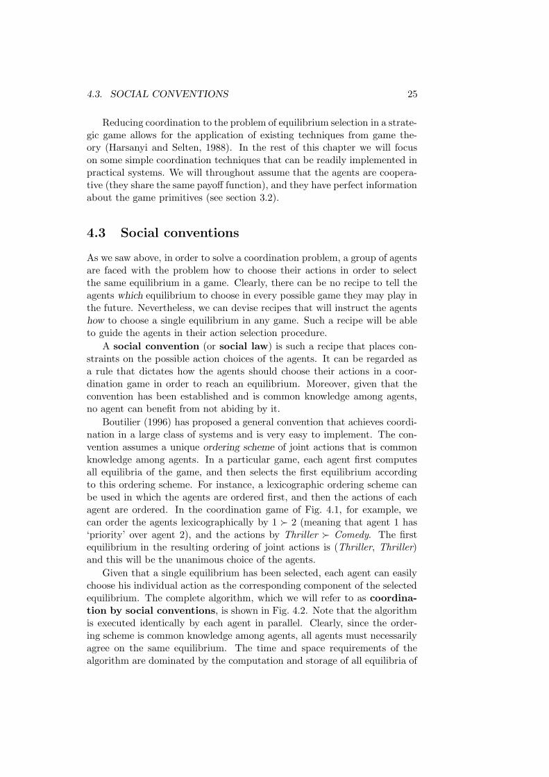
Given that a single equilibrium has been selected, each agent can easilychoose his individual action as the corresponding component of the selectedequilibrium. The complete algorithm, which we will refer to as coordina-tion by social conventions, is shown in Fig. 4.2. Note that the algorithmis executed identically by each agent in parallel. Clearly, since the order-ing scheme is common knowledge among agents, all agents must necessarilyagree on the same equilibrium. The time and space requirements of thealgorithm are dominated by the computation and storage of all equilibria of

26 CHAPTER 4. COORDINATION
For each agent i in parallelCompute all equilibria of the game.Order these equilibria based on a unique ordering scheme.Select the first equilibrium a∗ = (a∗−i, a
∗i ) in the ordered list.
Choose action a∗i .
End
Figure 4.2: Coordination by social conventions.
the game.
When the agents can perceive more aspects of the world state than justthe primitives of the game (actions and payoffs), one can think of moreelaborate ordering schemes for coordination. Consider the traffic game ofFig. 3.2(b), for example, as it is ‘played’ in the real world. Besides the gameprimitives, the state now also contains the relative orientation of the cars inthe physical environment. If we assume that the perception of the agentsfully reveals the state (full observability), then a simple convention is thatthe driver coming from the right will always have priority over the otherdriver in the lexicographic ordering. If we also order the actions by Cross �Stop, then coordination by social conventions implies that the driver fromthe right will cross the road first. Similarly, if traffic lights are available, thenthe state also includes the color of the light, in which case the establishedconvention is that the driver who sees the red light must stop.
4.4 Roles
Coordination by social conventions relies on the assumption that an agentcan compute all equilibria in a game before choosing a single one. However,computing equilibria can be expensive when the action sets of the agentsare large, therefore one would like to reduce the size of the action sets first.Such a reduction can have computational advantages in terms of speed, butmore importantly, it can simplify the equilibrium selection problem. In somecases, in the resulting subgame there is only one equilibrium left which istrivial to find.
A natural way to reduce the action sets of the agents is by assigningroles to the agents. Formally, a role can be regarded as a masking operatoron the action set of an agent, given a particular state. In practical terms,if an agent is assigned a role at a particular state, then some of the agent’sactions are deactivated at this state. In soccer for example, an agent that iscurrently in the role of defender cannot attempt to Score.
A role can facilitate the solution of a coordination game by reducing

4.4. ROLES 27
For each agent in parallelI = {}.For each role j = 1, . . . , n
For each agent i = 1, . . . , n with i /∈ ICompute the potential rij of agent i for role j.
EndAssign role j to agent i∗ = arg maxi{rij}.Add i∗ to I.
EndEnd
Figure 4.3: Role assignment.
it to a subgame where the equilibria are easier to find. For example, inFigure 4.1, if agent 2 is assigned a role that forbids him to select the actionThriller (e.g., he is under 16), then agent 1, assuming he knows the roleof agent 2, can safely choose Comedy resulting in coordination. Note thatthere is only one equilibrium left in the subgame formed after removing theaction Thriller from the action set of agent 2.
In general, suppose that there are n available roles (not necessarily dis-tinct), that the state is fully observable to the agents, and that the followingfacts are common knowledge among agents:
• There is a fixed ordering {1, 2, . . . , n} of the roles. Role 1 must beassigned first, followed by role 2, etc.
• For each role j there is a function that assigns to each agent i a po-tential rij that reflects how appropriate agent i is for the role j giventhe current state.
• Each agent can be assigned only one role.
Then, role assignment can be carried out by the algorithm shownin Fig. 4.3. Each role is assigned to the agent that has the highest potentialfor that role. This agent is eliminated from the role assignment process, anew role is assigned to another agent, and so on, until all agents have beenassigned a role.
The algorithm runs in time polynomial in the number of agents and roles,and is executed identically by each agent in parallel. Note that we haveassumed full observability of the state, and that each agent can computethe potential of each other agent. After all roles have been assigned, theoriginal coordination game is reduced to a subgame that can be furthersolved using coordination by social conventions. Recall from Fig. 4.2 that

28 CHAPTER 4. COORDINATION
the latter additionally requires an ordering scheme of the joint actions thatis common knowledge.
Like in the traffic example of the previous section, roles typically applyon states that contain more aspects than only the primitives of the strategicgame; for instance, they may contain the physical location of the agents inthe world. Moreover, the role assignment algorithm applies even if the stateis continuous; the algorithm only requires a function that computes poten-tials, and such a function can have a continuous state space as domain. Togive an example, suppose that in robot soccer we want to assign a particularrole j (e.g., attacker) to the robot that is closer to the ball than any otherteammate. In this case, the potential rij of a robot i for role j can be givenby a function of the form
rij = −||xi − xb||, (4.1)
where xi and xb are the locations in the field of the robot i and the ball,respectively.
4.5 Coordination graphs
As mentioned above, roles can facilitate the solution of a coordination gameby reducing the action sets of the agents prior to computing the equilibria.However, computing equilibria in a subgame can still be a difficult task whenthe number of involved agents is large; recall that the joint action space isexponentially large in the number of agents. As roles reduce the size ofthe action sets, we also need a method that reduces the number of agentsinvolved in a coordination game.
Guestrin et al. (2002a) introduced the coordination graph as a frame-work for solving large-scale coordination problems. A coordination graphallows for the decomposition of a coordination game into several smallersubgames that are easier to solve. Unlike roles where a single subgame isformed by the reduced action sets of the agents, in this framework varioussubgames are formed, each typically involving a small number of agents.
In order for such a decomposition to apply, the main assumption is thatthe global payoff function u(a) can be written as a linear combination ofk local payoff functions fj, each involving only few agents. For example,suppose that there are n = 4 agents, and k = 3 local payoff functions, eachinvolving two agents:
u(a) = f1(a1, a2) + f2(a1, a3) + f3(a3, a4). (4.2)
Here, f2(a1, a3) for instance involves only agents 1 and 3, with their actionsa1 and a3. Such a decomposition can be graphically represented by a graph(hence the name), where each node represents an agent and each edge cor-responds to a local payoff function. For example, the decomposition (4.2)can be represented by the graph of Fig. 4.4.

4.5. COORDINATION GRAPHS 29
PSfrag replacements
2
1
3
4
f1 f2
f3
Figure 4.4: A coordination graph for a 4-agent problem.
Let us now see how this framework can be used for coordination. Recallthat a solution to a coordination problem is a Pareto optimal Nash equilib-rium in the corresponding strategic game. By definition, such an equilibriumis a joint action a∗ that maximizes u(a). The key idea in coordination graphsis that the linear decomposition of u(a) allows for an iterative maximizationprocedure in which agents are eliminated one after the other.
We will illustrate this on the above example. We start by eliminatingagent 1 in (4.2). We collect all local payoff functions that involve agent 1,these are f1 and f2. The maximum of u(a) can then be written
maxa
u(a) = maxa2,a3,a4
{
f3(a3, a4) + maxa1
[
f1(a1, a2) + f2(a1, a3)]
}
. (4.3)
Next we perform the inner maximization over the actions of agent 1. Foreach combination of actions of agents 2 and 3, agent 1 must choose anaction that maximizes f1 +f2. This essentially involves computing the best-response function B1(a2, a3) of agent 1 (see section 3.4) in the subgameformed by agents 1, 2, and 3, and the sum of payoffs f1 + f2. The functionB1(a2, a3) can be thought of as a conditional strategy for agent 1, given theactions of agents 2 and 3.
The above maximization and the computation of the best-response func-tion of agent 1 define a new payoff function f4(a2, a3) = maxa1
[f1(a1, a2) +f2(a1, a3)] that is independent of a1. Agent 1 has been eliminated. Themaximum (4.3) becomes
maxa
u(a) = maxa2,a3,a4
[
f3(a3, a4) + f4(a2, a3)]
. (4.4)
We can now eliminate agent 2 as we did with agent 1. In (4.4), only f4
involves a2, and maximization of f4 over a2 gives the best-response functionB2(a3) of agent 2 which is a function of a3 only. This in turn defines a newpayoff function f5(a3), and agent 2 is eliminated. Now we can write
maxa
u(a) = maxa3,a4
[
f3(a3, a4) + f5(a3)]
. (4.5)
30 CHAPTER 4. COORDINATION
For each agent in parallelF = {f1, . . . , fk}.For each agent i = 1, 2, . . . , n
Find all fj(a−i, ai) ∈ F that involve ai.Compute Bi(a−i) = arg maxai
∑
j fj(a−i, ai).
Compute fk+i(a−i) = maxai
∑
j fj(a−i, ai).
Remove all fj(a−i, ai) from F and add fk+i(a−i) in F .EndFor each agent i = n, n− 1, . . . , 1
Choose a∗i ∈ Bi(a∗−i) based on a fixed ordering of actions.
EndEnd
Figure 4.5: Coordination by variable elimination.
Agent 3 is eliminated next, resulting in B3(a4) and a new payoff functionf6(a4). Finally, maxa u(a) = maxa4
f6(a4), and since all other agents havebeen eliminated, agent 4 can simply choose an action a∗
4 that maximizes f6.
The above procedure computes an optimal action only for the last elimi-nated agent (assuming that the graph is connected). For the other agents itcomputes only conditional strategies. A second pass in the reverse elimina-tion order is needed so that all agents compute their optimal (unconditional)actions from their best-response functions. Thus, in the above example,plugging a∗4 into B3(a4) gives the optimal action a∗
3 of agent 3. Similarly,we get a∗2 from B2(a
∗3) and a∗1 from B1(a
∗2, a
∗3), and thus we have computed
the joint optimal action a∗ = (a∗1, a∗2, a
∗3, a
∗4). Note that one agent may have
more than one best-response actions, in which case the first action can bechosen according to an a priori ordering of the actions of each agent thatmust be common knowledge.
The complete algorithm, which we will refer to as coordination byvariable elimination, is shown in Fig. 4.5. Note that the notation −ithat appears in fj(a−i, ai) refers to all agents other than agent i that areinvolved in fj, and it does not necessarily include all n−1 agents. Similarly,in the best-response functions Bi(a−i) the action set a−i may involve lessthan n− 1 agents. The algorithm runs identically for each agent in parallel.For that we require that all local payoff functions are common knowledgeamong agents, and that there is an a priori ordering of the action sets of theagents that is also common knowledge. The latter assumption is needed sothat each agent will finally compute the same joint action.
The main advantage of this algorithm compared to coordination by socialconventions in Fig. 4.2 is that here we need to compute best-response func-

4.6. NOTES AND FURTHER READING 31
tions in subgames involving only few agents, while computing all equilibriain Fig. 4.2 requires computing best-response functions in the complete gameinvolving all n agents. When n is large, the computational gains of variableelimination over coordination by social conventions can be significant.
For simplicity, in the above algorithm we have fixed the elimination orderof the agents as 1, 2, . . . , n. However, this is not necessary. Each agent run-ning the algorithm can choose a different elimination order, and the resultingjoint action a∗ will always be the same. The total runtime of the algorithm,however, will not be the same. Different elimination orders produce differ-ent intermediate payoff functions, and thus subgames of different size. Itturns out that computing the optimal elimination order (that minimizes theexecution cost of the algorithm) is NP-complete.
In all algorithms in this chapter the agents can coordinate their actionswithout the need to communicate with each other. As we saw, in all caseseach agent runs the same algorithm identically and in parallel, and coordi-nation is guaranteed as long as certain facts are common knowledge amongagents. In chapter 6 we will relax some of the assumptions of commonknowledge, and show how the above algorithms can be modified when theagents can explicitly communicate with each other.
4.6 Notes and further reading
The problem of multiagent coordination has been traditionally studied indistributed AI, where typically some form of communication is allowedamong agents (Jennings, 1996). (See also chapter 6.) The framework of‘joint intentions’ of Cohen and Levesque (1991) provides a formal charac-terization of multiagent coordination through a model of joint beliefs andintentions of the agents. Social conventions were introduced by Shohamand Tennenholtz (1992), as constraints on the set of allowed actions of asingle agent at a given state (similar to roles as in section 4.4). Boutilier(1996) extended the definition to include also constraints on the joint ac-tion choices of a group of agents, and proposed the idea of coordination bylexicographic ordering. A version of role assignment (that relies on com-munication) similar to Fig. 4.3 has been used by Castelpietra et al. (2000).Coordination graphs are due to Guestrin et al. (2002a). An application ofroles and coordination graphs in robot soccer can be found in (Kok et al.,2003).

32 CHAPTER 4. COORDINATION

Chapter 5
Common knowledge
In the previous chapters we generally assumed that the world state is fullyobservable to the agents. Here we relax this assumption and examine thecase where parts of the state are hidden to the agents. In such a partiallyobservable world an agent must always reason about his knowledge, and theknowledge of the others, prior to making decisions. We formalize the notionsof knowledge and common knowledge in such domains, and demonstratetheir implications by means of examples.
5.1 Thinking interactively
In order to act rationally, an agent must always reflect on what he knowsabout the current world state. As we saw in chapter 2, if the state is fullyobservable, an agent can perform pretty well without extensive deliberation.If the state is partially observable, however, the agent must first considercarefully what he knows and what he does not know before choosing anaction. Intuitively, the more an agent knows about the true state, the betterthe decisions he can make.
In a multiagent system, a rational agent must also be able to thinkinteractively, that is, to take into account the knowledge of the other agentsin his decision making. In addition, he needs to consider what the otheragents know about him, and also what they know about his knowledge. Inthe previous chapters we have often used the term common knowledgeto refer to something that every agent knows, that every agent knows thatevery other agent knows, and so on. For example, the social convention thata driver must stop in front of a red traffic light is supposed to be commonknowledge among all drivers.
In this chapter we will define common knowledge more formally, andillustrate some of its strengths and implications through examples. Oneof its surprising consequences, for instance, is that it cannot be commonknowledge that two rational agents would ever want to bet with each other!
33

34 CHAPTER 5. COMMON KNOWLEDGE
5.2 The puzzle of the hats
We start with a classical puzzle that illustrates some of the implications ofcommon knowledge. The story goes as follows:
Three agents (say, girls) are sitting around a table, each wearinga hat. A hat can be either red or white, but suppose that allagents are wearing red hats. Each agent can see the hat of theother two agents, but she does not know the color of her ownhat. A person who observes all three agents asks them in turnwhether they know the color of their hats. Each agent repliesnegatively. Then the person announces “At least one of you iswearing a red hat”, and then asks them again in turn. Agent 1says No. Agent 2 also says No. But when he asks agent 3, shesays Yes.
How is it possible that agent 3 can finally figure out the color of herhat? Before the announcement that at least one of them is wearing a redhat, no agent is able to tell her hat color. What changes then after theannouncement? Seemingly the announcement does not reveal anything new;each agent already knows that there is at least one red hat because she cansee the red hats of the other two agents.
Given that everyone has heard that there is at least one red hat, agent 3can tell her hat color by reasoning as follows: “Agent’s 1 No implies thateither me or agent 2 is wearing a red hat. Agent 2 knows this, so if my hathad been white, agent 2 would have said Yes. But agent 2 said No, so myhat must be red.”
Although each agent already knows (by perception) the fact that at leastone agent is wearing a red hat, the key point is that the public announce-ment of the person makes this fact common knowledge among the agents.Implicitly we have also assumed that it is common knowledge that eachagent can see and hear well, and that she can reason rationally. The puzzleis instructive because it shows the implications of interactive reasoning andthe strength of the common knowledge assumption.
5.3 Partial observability and information
Now we will try to formalize some of the concepts that appear in the puzzleof the hats. The starting point is that world state is partially observable tothe agents. Recall that in a partially observable world the perception of anagent provides only partial information about the true state, in the form ofa conditional probability distribution over states (see section 2.3). In thepuzzle of the hats this distribution is uniform over subsets of the state space,as we show next.

5.3. PARTIAL OBSERVABILITY AND INFORMATION 35
World statesa b c d e f g h
1 R R R R W W W WAgents 2 R R W W R R W W
3 R W R W R W R W
Figure 5.1: The eight world states in the puzzle of the hats.
In general, let S be the set of all states and s ∈ S be the current (true)state of the world. We assume that the perception of an agent i providesinformation about the state s through an information function
Pi : s 7→ Pi(s), (5.1)
where Pi(s) is a nonempty subset of S called the information set of agent iin state s. The interpretation of the information set is that when the truestate is s, agent i thinks that any state in Pi(s) could be the true state. Theset Pi(s) will always contain s, but essentially this is the only thing thatagent i knows about the true state. In the case of multiple agents, eachagent can have a different information function.
In the puzzle of the hats, a state is a three-component vector containingthe colors of the hats. Let R and W denote red and white. There are in totaleight states S = {a, b, c, d, e, f, g, h}, as shown in Fig. 5.1. By assumption,the true state is s = a. From the setup of the puzzle we know that thestate is partially observable to each agent; only two of the three hat colorsare directly perceivable by each agent. In other words, in any state s theinformation set of each agent contains two equiprobable states, those inwhich the only difference is in her own hat color. For instance, in states = a the information set of agent 2 is P2(s) = {a, c}, a two-state subsetof S.
As we mentioned above, the information set Pi(s) of an agent i containsthose states in S that agent i considers possible, if the true state is s. Ingeneral, we assume that the information function of an agent divides thestate space into a collection of mutually disjoint subsets, called cells, thattogether form a partition Pi of S. The information set Pi(s) for agent i intrue state s is exactly that cell of Pi that contains s, while the union of allcells in Pi is S.
Based on the information functions, we can compute the partitions ofthe agents in the puzzle of the hats:
Pt1 = {{a, e}, {b, f}, {c, g}, {d, h}}, (5.2)
Pt2 = {{a, c}, {b, d}, {e, g}, {f, h}}, (5.3)
Pt3 = {{a, b}, {c, d}, {e, f}, {g, h}}, (5.4)

36 CHAPTER 5. COMMON KNOWLEDGE
where t refers to the time step before any announcement took place. Clearly,in the true state s = a = RRR no agent knows her hat color, since thecorresponding cell of each partition contains two equiprobable states. Thus,agent 1 considers a and e possible, agent 2 considers a and c possible, andagent 3 considers a and b possible. (Note again that we know that the truestate is a but the agents in our puzzle do not.)
Now we make the additional assumption that all partitions are commonknowledge among the agents. In the case of homogeneous agents, for in-stance, this is not an unrealistic assumption; typically each agent will beaware of the perception capabilities of each other. In the puzzle of the hats,for example, it is reasonable to assume that all agents can see and hear welland that they are all rational. Then, simply the positioning of the agentsaround the table makes the above partitions common knowledge.
If the partitions are common knowledge, then in state a agent 1 thinksthat agent 2 may think that agent 3 might think that h = WWW is possible!Why is that? Note from (5.2) that in state a agent 1 thinks that either aor e could be the true state. But if e is the true state, then from (5.3)we see that agent 2 may consider g to be the true state. But then we seefrom (5.4) that agent 3 may consider h to be the true state. Note how theabove analytical framework allows for a fairly straightforward formulationof otherwise complicated statements.
Now the announcement of the person reveals that the true state is not h.This automatically changes the partitions of the agents:
Pt+11 = {{a, e}, {b, f}, {c, g}, {d}, {h}},
Pt+12 = {{a, c}, {b, d}, {e, g}, {f}, {h}},
Pt+13 = {{a, b}, {c, d}, {e, f}, {g}, {h}}.
(5.5)
Note that h has been disambiguated from d, f , and g, in the three partitions.The person then asks each agent in turn whether she knows the color of herhat. Agent 1 says No. In which case would agent 1 have said Yes? As wesee from the above partitions, only in state d would agent 1 have known herhat color. But the true state is a, and in this state agent 1 still considers epossible. (Compare this analysis with the logical reasoning of section 5.2.)
The reply of agent 1 eliminates state d from the set of candidate states.This results in a refinement of the partitions of agents 2 and 3:
Pt+21 = {{a, e}, {b, f}, {c, g}, {d}, {h}},
Pt+22 = {{a, c}, {b}, {d}, {e, g}, {f}, {h}},
Pt+23 = {{a, b}, {c}, {d}, {e, f}, {g}, {h}}.
(5.6)
Next agent 2 is asked. From her partition P t+22 we see that she would
have known her hat color only in state b or f (d and h are already ruled outby the previous announcements). However, in the true state a agent 2 still

5.4. A MODEL OF KNOWLEDGE 37
considers c possible, therefore she replies negatively. Her reply excludes band f from the set of candidate states, resulting in a further refinement ofthe partitions of agent 1 and 3:
Pt+31 = {{a, e}, {b}, {f}, {c, g}, {d}, {h}},
Pt+32 = {{a, c}, {b}, {d}, {e, g}, {f}, {h}},
Pt+33 = {{a}, {b}, {c}, {d}, {e}, {f}, {g}, {h}}.
(5.7)
The partition of agent 3 now contains only singleton cells, thus agent 3 cannow tell her hat color. Note that agents 1 and 2 still cannot tell their hatcolors. In fact, they will be unable to tell their har colors no matter howmany more announcements will take place; the partitions (5.7) cannot befurther refined. Interestingly, the above analysis would have been exactlythe same if the true state had been any one in the set {a, c, e, g}. (Try toverify this with logical reasoning.)
5.4 A model of knowledge
Any subset E of S is called an event. If for an agent i holds Pi(s) ⊆ Ein true state s, then we say that agent i knows1 E. Generalizing, theknowledge function of an agent i is defined as
Ki(E) = {s ∈ S : Pi(s) ⊆ E}. (5.8)
That is, for any event E, the set Ki(E) contains all states in which agent iknows E. It is not difficult to see that Ki(E) can be written as the unionof all cells of Pi that are fully contained in E. In the puzzle of the hats, forexample, in the final partitions (5.7) holds K1({a, e, c}) = {a, e}, while forthe event E = {a, c, e, g} holds Ki(E) = E for all i = 1, 2, 3.
An event E ⊆ S is called self-evident to agent i if E can be writtenas a union of cells of Pi. For example, in (5.7) the event E = {a, c, e, g} isself-evident to all three agents. As another example, suppose that the statespace consists of the integer numbers from 1 to 8, the true state is s = 1,and two agents have the following partitions:
P1 = {{1, 2}, {3, 4, 5}, {6}, {7, 8}},
P2 = {{1, 2, 3}, {4}, {5}, {6, 7, 8}}.(5.9)
1This definition of knowledge is slightly different from the one used in epistemic
logic. There an agent is said to know a fact φ if φ is true in all states the agent considerspossible. In the event-based framework, an agent knows an event E if all the states theagent considers possible are contained in E. Intuitively, if a fact φ is true in all s ∈ E,and the agent knows E, then the agent also knows φ (since φ is true in all states the agentconsiders possible). Fagin et al. (1995, sec. 2.5) show that the two approaches, logic-basedand event-based, are in fact equivalent.

38 CHAPTER 5. COMMON KNOWLEDGE
In s = 1 agent 1 thinks that {1, 2} are possible. Agent 1 also thinks thatagent 2 may think that {1, 2, 3} are possible. Furthermore, agent 1 thinksthat agent 2 may think that agent 1 might think that {1, 2} or {3, 4, 5}are possible. But nobody needs to think beyond 5. In this example, theevent {1, 2, 3, 4} is self-evident to agent 2, while the event {1, 2, 3, 4, 5} isself-evident to both agents.
We can now formalize the notion of common knowledge. For simplicity,the first definition is formulated for only two agents.
Definition 5.4.1. An event E ⊆ S is common knowledge between agents1 and 2 in true state s ∈ S, if s is a member of every set in the infinitesequence K1(E), K2(E), K1(K2(E)), K2(K1(E)), . . ..
Definition 5.4.2. An event E ⊆ S is common knowledge among a groupof agents in true state s ∈ S, if s is a member of any set F ⊆ E that isself-evident to all agents.
It turns out that the two definitions are equivalent (Osborne and Ru-binstein, 1994, prop. 74.2). However, the second definition is much easierto apply; it only requires computing self-evident sets which are unions ofpartition cells and thus easy to find. For instance, in the above examplethe event E = {1, 2, 3, 4, 5} is common knowledge between the two agentsbecause E is self-evident to both of them and the true state s = 1 belongsto E. Similarly, in the puzzle of the hats, in the final partitions (5.7), andwith true state s = a, the event E = {a, c, e, g} is common knowledge amongall three agents.
5.5 Knowledge and actions
So far we have discussed how the perceptions of the agents are related tothe world states through the information functions, and what it means tosay that an event is common knowledge among a group of agents. We nowextend the framework to incorporate also the actions of the agents.
In section 2.2 we defined a memoryless policy π of an agent as a mappingfrom perceptions to actions (2.2). Equivalently, in the current frameworkwe can assume that the policy of an agent i with information function Pi isa mapping from information sets to actions:
πi : Pi(s) 7→ ai (5.10)
where s is the current state. For example, in the puzzle of the hats, a replyYes or No of an agent to the question “Do you know your hat color?” canbe regarded as an action taken by the agent given her current information.In the final partitions (5.7), agent 1 will reply No given her information set{a, e} and agent 3 will reply Yes given her information set {a}.

5.5. KNOWLEDGE AND ACTIONS 39
Let E be the set of states in which agent i takes a particular action ai,that is, E = {s ∈ S : πi(Pi(s)) = ai}. If another agent j knows the policyand the information function of agent i, then agent j will know that agent itakes action ai in state s if and only if agent j knows E. Similarly, assumingthat the policy and the information function of agent i is common knowledge,then it will be common knowledge in s that agent i takes action ai if andonly if E is common knowledge.
Let us also assume that for two information sets E and F of an agent ithe following ‘union-consistency’ property holds:
πi(E) = πi(F ) =⇒ πi(E) = πi(E ∪ F ). (5.11)
In other words, if an agent is taking the same action in two different infor-mation sets, then he must be taking the same action in their union as well.In the puzzle of the hats, for instance, if an agent answers No if she knowsthat the true state s is in E, and she also answers No if she knows thats ∈ F , then she will also answer No if she only knows that s ∈ E ∪ F .
Given the above, it turns out that for a group of agents with potentiallydifferent information functions, the following result holds:
Proposition 5.5.1. If the agents run the same policy π, and it is commonknowledge in the current state what actions the agents are taking, then theagents must be taking the same actions.
Proof. The fact that in the current state the action ai of an agent i iscommon knowledge among all agents implies that there must be a set E ⊆ Sthat is common knowledge among all agents, and in all states of which agent iwould take action ai, that is, π(Pi(s)) = ai for all s ∈ E. Since E is commonknowledge among the agents, it must be self-evident to all agents, thus wecan write E =
⋃
s∈E Pi(s) for all i. But then (5.11) implies that π(E) = ai
for all i, therefore all ai must be equal.
As noted by Geanakoplos (1992), a surprising consequence of this propo-sition is that, for instance, rational agents would never want to bet witheach other if their bets are common knowledge. Moreover, this is true evenif the agents have different information about the current state. Betting isequivalent to deciding whether a random variable has positive or negativeexpectation. For expectations of random variables the union-consistencyproperty (5.11) holds, therefore, assuming the agents are of the same ‘mind’,proposition 5.5.1 applies.
Finally, there is the question of how the agents can actually reach com-mon knowledge of actions. As we saw in the puzzle of the hats, the publicannouncement of the action of each agent allows for a stepwise refinementof the partitions of the agents. At some point in time this refinement stopsbecause there are only a finite number of states. At this point it will be
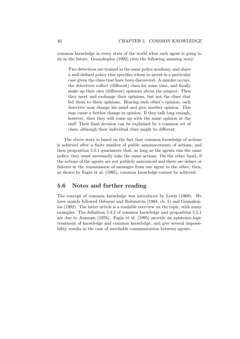
40 CHAPTER 5. COMMON KNOWLEDGE
common knowledge in every state of the world what each agent is going todo in the future. Geanakoplos (1992) cites the following amusing story:
Two detectives are trained in the same police academy, and sharea well-defined policy that specifies whom to arrest in a particularcase given the clues that have been discovered. A murder occurs,the detectives collect (different) clues for some time, and finallymake up their own (different) opinions about the suspect. Thenthey meet and exchange their opinions, but not the clues thatled them to these opinions. Hearing each other’s opinion, eachdetective may change his mind and give another opinion. Thismay cause a further change in opinion. If they talk long enough,however, then they will come up with the same opinion at theend! Their final decision can be explained by a common set ofclues, although their individual clues might be different.
The above story is based on the fact that common knowledge of actionsis achieved after a finite number of public announcements of actions, andthen proposition 5.5.1 guarantees that, as long as the agents run the samepolicy, they must necessarily take the same actions. On the other hand, ifthe actions of the agents are not publicly announced and there are delays orfailures in the transmission of messages from one agent to the other, then,as shown by Fagin et al. (1995), common knowledge cannot be achieved.
5.6 Notes and further reading
The concept of common knowledge was introduced by Lewis (1969). Wehave mainly followed Osborne and Rubinstein (1994, ch. 5) and Geanakop-los (1992). The latter article is a readable overview on the topic, with manyexamples. The definition 5.4.2 of common knowledge and proposition 5.5.1are due to Aumann (1976). Fagin et al. (1995) provide an epistemic-logictreatment of knowledge and common knowledge, and give several impossi-bility results in the case of unreliable communication between agents.

Chapter 6
Communication
In this chapter we address the issue of multiagent communication. We viewcommunication as a means for the agents to revise their knowledge, and webriefly review communicative acts, a formal framework for agent interaction.Then we explain how an agent can compute the value of a communicativeact using the framework of Bayesian games. Finally, we show how communi-cation can be effectively used for multiagent coordination, by appropriatelymodifying the coordination algorithms of chapter 4.
6.1 Communicating agents
Multiagent interaction is often associated with some form of communica-tion. We employ communication in most of our daily social activities, forcooperatively solving a problem, for negotiating with others, or simply forexchanging knowledge with others. As we saw in the puzzle of the hatsin chapter 5, by communicating their answers to each other, the agents wereable to form more accurate statements about the problem, and eventuallysolve it.
When we talk about computational agents, communication involves sev-eral levels of abstraction. On the lower, ‘network’ level, one would like tomake sure that the messages that are communicated among the agents ar-rive safely and timely at their destination. For that, several well-studiedformalisms and protocols exist in the distributed systems literature (Tanen-baum and van Steen, 2001). On an intermediate, ‘language’ level, one wouldlike to have a basic set of language primitives and a standardized format forexchanging these primitives, so that agents that speak the same languagecan easily understand each other. Finally, on a high, ‘application’ level, onewould like to effectively use communication for solving standard multiagentproblems, like coordination or negotiation.
Next we will briefly address the issues of defining appropriate languageprimitives, and using communication for multiagent coordination.
41

42 CHAPTER 6. COMMUNICATION
6.2 Communicative acts
As we saw in the previous chapters, a world state is characterized by a num-ber of agents, the available actions and the payoffs of the agents if the latterare involved in a strategic game, and other aspects of the external environ-ment (e.g., the color of a traffic light in a traffic coordination problem). Insome cases, as we saw in section 4.4, some of the actions of an agent may bedeactivated in a particular state because this agent is assigned a particularrole. Similarly, if the world state is partially observable to the agents, eachagent may possess different levels of knowledge about the true state, as wesaw in chapter 5; if the true state is s, an agent i may consider all states inhis information set Pi(s) as candidate true states.
A formal way to describe communication is by treating each commu-nication primitive as an action that updates the knowledge of an agentabout aspects of the state like those described above. The communica-tion primitives that are exchanged among agents are typically referred to ascommunicative acts or speech acts. Some of the most common types ofcommunicative acts are the following (as they could be applied, for example,by an agent in the traffic coordination problem of Fig. 3.2):
Informing about some aspects of the current state, “The traffic light is outof order,” or about what an agent knows, “The car from the right haspriority.”
Querying aspects of the state that are hidden, “Does your traffic lightwork?” or “Do you consider crossing?” or “What is the convention inthis country?”
Committing to a particular action, “I will cross.”
Prohibiting an action, “You may not cross.”
Directing an agent to do an action, “Cross!”
Each communicative act can affect the knowledge of the agents in adifferent way. For example, an informing act can reduce the uncertainty ofan agent about the current state by eliminating candidate states from hisinformation set. In the puzzle of the hats, for example, if at the beginningagent 1 says “The hat of agent 3 is red”, then, given that agent 1 is truthful,the information set of agent 3 is transformed from {a, b} to {a}, and thepartitions of all agents change accordingly. Similarly, the answer No of anagent i to the query “Do you know your hat color?” is a communicativeact that informs the other agents about the current knowledge of agent iregarding the true state, and results in a refinement of their partitions aswe saw in section 5.3.

6.3. THE VALUE OF COMMUNICATION 43
A committing communicative act, on the other hand, can be used forinforming about the chosen course of action of an agent. We have alreadyseen an example where an agent commits to choosing a specific course ofaction: in the backward pass of the variable elimination algorithm of Fig. 4.5,an agent that computes its optimal action according to its best-responsefunction and given the optimal actions of the other agents so far, implicitlycommits to taking this action. In section 6.4, this communicative act willbe made more explicit by having each agent communicate its chosen actionto the other agents.
Similar interpretations can be given to the other communicative acts. Forinstance, a prohibiting act can have the same effect as a role (see section 4.4),by enforcing the deactivation of some actions of an agent in a particularsituation. A directing act may apear in an organizational structure of theagents in which an agent with more authority can give commands to theother agents.
Recently, several agent communication languages have been pro-posed in the agents community, aiming at standardizing the multiagentcommunication process (Labrou et al., 1999). The two most notable onesare KQML and FIPA ACL, each using a slightly different syntax and set ofcommunicative acts. Unfortunately, many dialects of these languages havealready appeared, and the languages seem not to conform with other stan-dards (for example, in the Internet). As it is often the case, we might see inthe future new language standards emerging directly from applications.
6.3 The value of communication
As we mentioned above, a communicative act can be viewed as an actionthat changes the knowledge state of the involved agents. Given a set ofavailable communicative acts, an agent in a particular state is faced withthe question which act to use and whom to communicate it to. Naturally,we would like to assign a value to a communicative act as an indicator of thegoodness of this act, just like a Q-value measures the goodness of a regularaction of an agent (see section 2.4). This would allow an agent to selectthe most appropriate communicative act per case. But where should thesevalues come from?
A formal framework that allows us to properly define the value of com-munication is a Bayesian game. This model combines the strategic gameof chapter 3 with the partial observability concepts of chapter 5. In par-ticular, we assume a number of agents, a set S of world states, and aninformation function for each agent i that gives rise to a partition Pi of S,different for each agent. We also assume that each state s ∈ S occurs withsome (prior) probability that is assumed equal for all agents, and that itdefines a strategic game Gs with corresponding payoffs.

44 CHAPTER 6. COMMUNICATION
L R
U 2, 2 1, 0
D 0, 1 0, 0
L R
U 0, 0 0, 1
D −1, 0 2, 2
Ga (probability 0.7) Gb (probability 0.3)
Figure 6.1: A Bayesian game defined by two strategic games, Ga and Gb.
We will explain by an example how the model of a Bayesian game can beused for defining the value of a communicative act. Suppose there are twoagents, the state space is S = {a, b}, and the information partitions of theagents are P1 = {{a}, {b}} and P2 = {{a, b}} and they are common knowl-edge among the agents. In any true state s, agent 1 knows s, but agent 2does not know s, and agent 1 knows that agent 2 does not know s. Supposealso that state a occurs with probability 0.7 and state b with probability 0.3,and let each of them define a strategic game as shown in Fig. 6.1.
In this problem, the actions of the agents should depend on what stateis actually realized, in other words, which one of Ga or Gb actually applies.Note that, contrary to the coordination problems of chapter 4 where theagents had to choose among several equilibria, here each of the two gameshas a single equilibrium which is trivial to find; in s = a the agents shouldchoose (U, L ), and in s = b they should choose (D, R ). However, agent 2does not know what the true state is, and thus it is difficult for him topredict the action of agent 1 and find the correct equilibrium.
Given the partial knowledge of the agents about the true state, the ra-tional joint action (Nash equilibrium) for the agents is (U, L ) which gives toeach of them expected payoff 0.7∗2+0.3∗0 = 1.4. Now, if in any true state sagent 1 informs agent 2 about s with a communicative act, the partition ofagent 2 will read P2 = {{a}, {b}} and the agents can now safely choose thecorrect equilibrium for each value of s. This gives to each of them payoff 2.The difference 2−1.4 = 0.6 of the expected payoffs of each agent before andafter communication defines the value of the corresponding communicativeact.
In a similar manner an agent can compute the value of all its availablecommunicative acts in some situation, and then choose the one with thehighest value. In practice, however, taking an optimal decision about whatand with whom to communicate may require computational resources thatgo beyond the capacity of an agent. For a bounded rational agent withmemory and time restrictions, there is always a trade-off between choosinga good communicative act (or any other action) and choosing it quickly. Wecould also think of having each agent broadcast its private information toall other agents in every time step, but this could lead to communicationbottlenecks or other effects.

6.4. COORDINATION VIA COMMUNICATION 45
For each agent i in parallelIf i 6= 1
Wait until all actions (a∗1, . . . , a
∗i−1) are received.
EndCompute an equilibrium that contains (a∗
1, . . . , a∗i−1, . . .).
Choose component a∗i from this equilibrium.
Broadcast action a∗i to all agents i + 1, . . . , n.
End
Figure 6.2: Coordination by broadcast.
6.4 Coordination via communication
In chapter 4 we studied several coordination algorithms for cooperativeagents. These algorithms relied on several common knowledge assumptions.In this section we relax some of these assumptions, and show how the algo-rithms can be modified to explicitly take communication into account. Anadvantage of using communication is that an agent does not need to predictthe actions of all other agents at the equilibrium anymore.
Social conventions
When communication is not available, coordination by social conventions isbased on an ordering scheme of joint actions that has been a priori definedand is common knowledge among agents. As we explained in section 4.3,such an ordering scheme can be realized in a lexicographic manner, by firstordering the agents, and then the actions of the agents.
When communication is available, we only need to impose an orderingi = 1, . . . , n of the agents that is common knowledge. Coordination can nowbe achieved by the algorithm of Fig. 6.2. Each agent i (except agent 1) waitsuntil all previous agents 1, . . . , i−1 in the ordering have broadcast their cho-sen actions. Then, agent i computes its component of the equilibrium thatagrees with the choices of the previous agents, that is (a∗
1, . . . , a∗i−1, a
∗i , . . .),
and broadcasts a∗i to all agents that have not chosen an action yet. Note
that, unlike the communication-free coordination algorithm of Fig. 4.2 whereeach agent runs the same procedure identically and in parallel, here the fixedordering of the agents together with the wait/broadcast primitives result ina synchronized sequential execution order.
Note that in the above algorithm an agent needs to compute only its owncomponent of any equilibrium that is consistent with the previously broad-cast actions, while its communication-free counterpart of Fig. 4.2 requiresthat each agent computes all equilibria in the game which can be costly.

46 CHAPTER 6. COMMUNICATION
For each agent i in parallelI = {}.For each role j = 1, . . . , n
Compute the potential rij of agent i for role j.Broadcast rij to all agents.
EndWait until all ri′j, for j = 1, . . . , n, are received.For each role j = 1, . . . , n
Assign role j to agent i∗ = arg maxi′ /∈I{ri′j }.Add i∗ to I.
EndEnd
Figure 6.3: Role assignment by broadcast.
Role assignment
The role assignment algorithm of Fig. 4.3 was based on the assumptionthat each agent is able to compute the potential of each other agent fora particular role. In practice, however, this is not always possible; in apartially observable domain, a potential function may require elements ofthe state that are only privately perceived by an agent (a soccer robot mayknow how close it is to the ball, but may not know how close its teammatesare to the ball). In some applications it seems more natural to have eachagent compute by itself how suitable it is for a particular role.
When communication is available, role assignment requires that an agentcomputes only its own potentials for the set of roles, and then broadcaststhem to the rest of the agents. The agent then waits for all other potentialsto arrive, and finally computes the assignment of roles to agents as in thecommunication-free role assignment algorithm of Fig. 4.3. Here too we as-sume a fixed ordering j = 1, . . . , n of the set of roles and a potential functionfor each role that are common knowledge among the agents. The algorithmis shown in Fig. 6.3. Note that the broadcast of the potentials to all agentsallows each agent to compute the full assignment of all roles to all agents.As in Fig. 4.3, agent i will be assigned role j when i∗ = i, which will occuronly once: every agent i∗ that is assigned a role is added to I, and is notconsidered again in the set of candidates i′ for a new role.
Concerning the computational requirements, each agent now needs tocompute only O(n) (its own) potentials instead of O(n2) in the algorithmof Fig. 4.3, but this will be compensated by the total number O(n2) ofpotentials that need to be broadcast and processed by the agents. Notethat the maximization step over {ri′j} is the same in both algorithms.
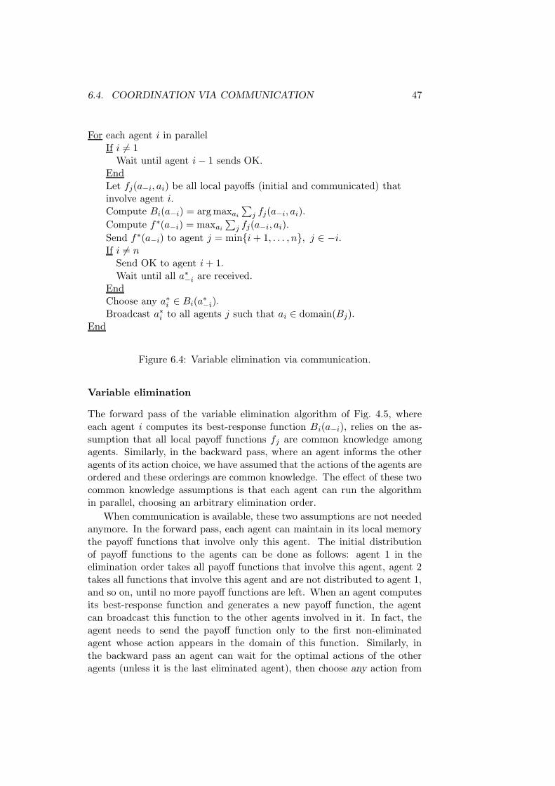
6.4. COORDINATION VIA COMMUNICATION 47
For each agent i in parallelIf i 6= 1
Wait until agent i− 1 sends OK.EndLet fj(a−i, ai) be all local payoffs (initial and communicated) thatinvolve agent i.Compute Bi(a−i) = arg maxai
∑
j fj(a−i, ai).
Compute f ∗(a−i) = maxai
∑
j fj(a−i, ai).
Send f∗(a−i) to agent j = min{i + 1, . . . , n}, j ∈ −i.If i 6= n
Send OK to agent i + 1.Wait until all a∗
−i are received.EndChoose any a∗i ∈ Bi(a
∗−i).
Broadcast a∗i to all agents j such that ai ∈ domain(Bj).End
Figure 6.4: Variable elimination via communication.
Variable elimination
The forward pass of the variable elimination algorithm of Fig. 4.5, whereeach agent i computes its best-response function Bi(a−i), relies on the as-sumption that all local payoff functions fj are common knowledge amongagents. Similarly, in the backward pass, where an agent informs the otheragents of its action choice, we have assumed that the actions of the agents areordered and these orderings are common knowledge. The effect of these twocommon knowledge assumptions is that each agent can run the algorithmin parallel, choosing an arbitrary elimination order.
When communication is available, these two assumptions are not neededanymore. In the forward pass, each agent can maintain in its local memorythe payoff functions that involve only this agent. The initial distributionof payoff functions to the agents can be done as follows: agent 1 in theelimination order takes all payoff functions that involve this agent, agent 2takes all functions that involve this agent and are not distributed to agent 1,and so on, until no more payoff functions are left. When an agent computesits best-response function and generates a new payoff function, the agentcan broadcast this function to the other agents involved in it. In fact, theagent needs to send the payoff function only to the first non-eliminatedagent whose action appears in the domain of this function. Similarly, inthe backward pass an agent can wait for the optimal actions of the otheragents (unless it is the last eliminated agent), then choose any action from
48 CHAPTER 6. COMMUNICATION
its best-response action set, and finally broadcast this action to all agentsthat need it in their best-response functions.
The complete algorithm is shown in Fig. 6.4. A crucial difference withthe communication-free variable elimination algorithm of Fig. 4.5 is thathere the elimination order i = 1, . . . , n of the agents is a priori fixed andis common knowledge among the agents. The OK signal is required forsynchronization, ensuring an execution order of the algorithm according tothe elimination order of the agents.
In terms of complexity, the forward pass is slightly slower than in thecommunication-free case, because here the generated payoffs need to be com-municated to the other involved agents. On the other hand, when commu-nication is available the backward pass is fully asynchronous. One can alsothink of asynchronous versions of the forward pass in which many agentsare simultaneously eliminated. This would require some additional book-keeping for storing the pairwise dependencies between agents.
6.5 Notes and further reading
Speech acts have been studied by Searle (1969). Bayesian games are brieflycovered in (Osborne and Rubinstein, 1994). The role assignment algorithmof Fig. 6.3 has been proposed by Castelpietra et al. (2000). Gmytrasiewiczand Durfee (2001) analyze communication in a Bayesian game setting wherethe agents model the knowledge of each other recursively. The latter providealso a framework for multiagent coordination. Among early approaches indistributed AI to communication-based coordination is the ‘contract net pro-tocol’ of Smith (1980) where tasks are dynamically distributed among agentsusing a bidding mechanism (see also chapter 7), and the ‘partial global plan-ning’ algorithm of Durfee and Lesser (1987) and Decker and Lesser (1995)in which agents exchange and refine local plans in order to reach a commongoal. The variable elimination algorithm of Fig. 6.4 is due to Guestrin et al.(2002a).

Chapter 7
Mechanism design
In this chapter we study the problem of mechanism design, which is thedevelopment of agent interaction protocols that explicitly take into accountthe fact that the agents may be self-interested. We discuss the revelationprinciple and the Groves-Clarke family of mechanisms that allow us to buildsuccessful protocols in a wide variety of practical problems.
7.1 Self-interested agents
In the previous chapters we mainly studied multiagent systems that consistof cooperative agents. The fact that the agents work cooperatively for a com-mon goal allowed us to develop algorithms, like the coordination algorithmsof chapter 4 and 6, in which the agents are assumed to be sincere to eachother and behave as instructed. A soccer agent, for instance, would neverviolate a protocol that assigns roles to teammates (see Fig. 4.3), becausethis could potentially harm the performance of his team.
In many practical applications, however, we have to deal with self-interested agents, for example, agents that act on behalf of some ownerthat wants to maximize his or her own profit. A typical example is a softwareagent that participates in an electronic auction on the Internet. Developingan algorithm or protocol for such a system is a much more challenging taskthan in the cooperative case. First, we have to motivate an agent to par-ticipate in the protocol, which is not a priori the case. Second, we have totake into account the fact that an agent may try to manipulate the protocolfor his own interest, leading to suboptimal results. The latter includes thepossibility that the agent may lie, if needed.
The development of protocols that are stable (nonmanipulable) and in-dividually rational for the agents (no agent is worse off by participating) isthe subject of mechanism design or implementation theory. As wewill see next, a standard way to deal with the above two problems is toprovide payments to the agents in exchange for their services.
49

50 CHAPTER 7. MECHANISM DESIGN
7.2 The mechanism design problem
In chapter 3 we used the model of a strategic game to describe a situationin which a group of agents interact with each other. The primitives ofsuch a game are the action sets Ai and the payoff functions ui(a) of theagents, for i = 1, . . . , n, where ui(a) reflects the preference of agent i forthe joint action a. Moreover, for any profile of payoff functions, a solutionconcept (e.g., Nash equilibrium) allows us to make predictions over the setof outcomes that may result when the game is played. Our standpointin chapter 3 was that of an external observer who wants to know the outcomeof a game, but cannot affect this outcome in any way.
In mechanism design we go one step further. Here we assume a set Oof possible outcomes over which a number of agents form preferences. Ourtask is to design a game that, when played by the agents, brings about adesired outcome from O. In this framework we therefore use a game as atool for achieving our design goals. An outcome can be practically anything,for example, the assignment of a resource to an agent. The main difficultyin mechanism design is that we often do not know the preferences of theagents in advance.
More formally, in each world state we assume that each agent i receivessome private information θi ∈ Θi, called the type of the agent, which isnot revealed to the other agents or to us (the mechanism designer). We canthink of a profile θ = (θi) of agent types as a world state, and in each state θagent i considers possible all states in which his type is θi (see chapter 5).Moreover, we assume that the type of an agent fully specifies the preferencesof this agent over the set of outcomes o ∈ O. In particular, each agent i hasa valuation function νi(o, θi), that is parametrized on θi, such that agent iin type θi prefers outcome o to o′ if and only if νi(o, θi) > νi(o
′, θi). We willassume that in each state θ we know the valuation function of each agent i(but not his type), and this fact is common knowledge among all agents.
In a mechanism design problem we hold a social choice function f(θ)that, for each profile θ = (θi) of agent types, produces a desired outcomeo = f(θ). We can think of f as an algorithm that solves an optimizationproblem: given n inputs θ = (θi), the function f computes an outcome othat maximizes a functional over the set of agents valuations. A typicalcase, which we will examine further in section 7.4, is to select the outcomethat maximizes the sum of the agents valuations given their types:
f(θ) = arg maxo∈O
n∑
i=1
νi(o, θi). (7.1)
Such a social choice function is called allocatively-efficient.
Implementing a social choice function would be easy if we had full ob-servability of the state θ. Then we could just use θ in (7.1) and compute

7.2. THE MECHANISM DESIGN PROBLEM 51
the desired optimal outcome (assuming, of course, that we have a tractablealgorithm for doing this). However, as we saw above, θi is revealed onlyto agent i. One option would be to ask each agent to tell us his type, butthere is no guarantee that an agent will report his true type! Recall thateach agent i forms his own preferences over outcomes, given by his valuationfunction νi(o, θi) with θi his true type. If by reporting a false type θi 6= θi anagent i expects to receive higher payoff than by reporting θi, then this agentmay certainly consider lying. As we mentioned in the introduction, in mech-anism design our starting point is that the agents are self-interest. Viewedfrom a computational perspective, we can therefore characterize mechanismdesign as follows:
Definition 7.2.1. Mechanism design is the development of efficient algo-rithms for optimization problems in which some of the parameters of theobjective function are in the control of agents that have different prefer-ences for different solutions.
The challenge is therefore to design mechanisms that steer the agentstoward selecting the desired o = f(θ) by themselves, for any profile of theirtypes. However, we first need to motivate the agents to participate in sucha mechanism—participation is not a priori the case! To accomplish this,we define a payment function p(o) that associates with each outcome oa profile p(o) = (pi(o)) of payments, so that agent i receives payment pi(o)when o occurs. The valuation function together with the payment functiondefine the payoff function of an agent (we assume that payments andvaluations are expressed in the same units):
ui(o, θi) = νi(o, θi) + pi(o). (7.2)
A mechanism that implements a social choice function f(θ) where no agentis worse off by participating, that is, ui(f(θ), θi) ≥ 0 for all i and all θ, iscalled individually rational.
We focus here on simple mechanisms in the form of a strategic gameM = (Ai, g, p) where Ai is a set of available actions for agent i, g(a) = ois an outcome function that maps a joint action a to an outcome o ∈ O,and p = p(o) is a payment function that controls the agents preferencesthrough (7.2). When the agents play the game M, we expect them tochoose a joint action a∗(θ) = (a∗i (θi)) according to some solution concept,where the action a∗
i (θi) of an agent i will typically depend on his type θi.This joint action is then mapped through g to an outcome g(a∗(θ)) whichwe want to equal f(θ). As solution concept we will consider the following:
Definition 7.2.2. A joint action a∗ = (a∗i ) is an equilibrium in dominantactions if for every agent i holds
ui(a−i, a∗i ) ≥ ui(a−i, ai) (7.3)
for all joint actions (a−i, ai).
52 CHAPTER 7. MECHANISM DESIGN
Our choice of such a solution concept is motivated by the fact that wewant to design a mechanism in which each agent i can compute his optimalaction a∗i without having to worry about the actions of the other agents.In terms of predictive power for the solutions of a game, an equilibriuma∗ = (a∗i ) in dominant actions is weaker than both a Nash equilibrium and anequilibrium computed by iterated elimination of strictly dominated actions(see chapter 3). However, in the context of mechanism design, the existenceof such an equilibrium guarantees that every (rational) agent will adhere toit, even if he has no information about the action choice of the other agents.Such an equilibrium solution is also very attractive computationally, becausean agent does not need to consider the actions of the other agents anymore.Summarizing, the mechanism design problem can be defined as follows:
Definition 7.2.3 (The mechanism design problem). Given a set ofoutcomes o ∈ O, a profile of valuation functions νi(o, θi) parametrized by θi,and a social choice function f(θ), find appropriate action sets Ai, an outcomefunction g(a) = o, and a payment function p(o), such that for any profile θ =(θi), and for payoff functions ui(o, θi) defined via (7.2), holds g(a∗(θ)) = f(θ)where a∗(θ) = (a∗i (θi)) is an equilibrium solution in dominant actions of thestrategic game M = (Ai, g, p). In this case we say that the mechanism Mimplements the social choice function f in dominant actions.
Example: second-price auction
Consider the following mechanism design problem (an auction). We have nagents and an item (e.g., a resource in a computer network). We want toassign the item to the agent that values it most, but we do not know thetrue valuations of the agents. In this example, the type θi of an agent is hisvaluation, with θi ∈ IR+, and an outcome o ∈ {1, . . . , n} is the index of theagent to whom the item is assigned. The valuation function of an agent iwith type i is νi(o, θi) = θi if o = i and zero otherwise. The social choicefunction is f(θ1, . . . , θn) = arg maxi{θi} (note that this is a simplified versionof (7.1)). If we do not include a payment function, that is pi(o) = 0 for all i,then a mechanismM1 = (Ai, g, 0) that implements f is always individuallyrational because for an agent i holds ui(o, θi) = νi(o, θi) = θi ≥ 0.
Suppose now that we incorporate a payment function p(o) such that theagent who receives the item must pay tax (negative payment) equal to thesecond highest valuation, whereas the other agents do not have to pay any-thing. In this case, the payoff function of an agent i with valuation θi equalsui(o, θi) = θi + pi if o = i and zero otherwise, where pi = −maxj 6=i{θj}.A mechanism M2 = (Ai, g, p) with such a payment function p that imple-ments f is still individually rational because for the winning agent k holdsuk(k, θk) = θk −maxj 6=k{θj} = maxj{θj} − maxj 6=k{θj} ≥ 0, while for theother agents j 6= k holds uj(k, θj) = 0.

7.3. THE REVELATION PRINCIPLE 53
7.3 The revelation principle
Looking at definition 7.2.3, mechanism design seems a formidable task. Ourdesign options can in principle involve all possible action sets Ai, all possibleoutcome functions g, and all kinds of payments p that we could provide tothe agents. Searching in the space of allM = (Ai, g, p) for a mechanism thatimplements f would be infeasible. Fortunately, there is a theorem that tellsus that we do not need to search in the space of all possible mechanisms.
Proposition 7.3.1 (Revelation principle). If a social choice function fis implementable in dominant actions by a mechanismM = (Ai, g, p), thenf is also implementable in dominant actions by mechanism M′ = (Θi, f, p)where each agent is simply asked to report his type. Moreover, the dominantaction of agent i in M′ is to report his true type θi.
Proof. Suppose truth-telling is not a dominant action in M′. Then theremust be a profile of reported types θ = (θi) for which
ui(f(θ−i, θi), θi) > ui(f(θ−i, θi), θi). (7.4)
If f is implementable by M in dominant actions, then f(θ) = g(a∗(θ)) forall θ, where a∗(θ) = (a∗i (θi)) is an equilibrium in dominant actions in M.We can therefore rewrite (7.4) as
ui(g(a∗−i(θ−i), a∗i (θi)), θi) > ui(g(a∗−i(θ−i), a
∗i (θi)), θi) (7.5)
which contradicts the fact that a∗i (θi) is a dominant action inM. Thus the
profile of true types θ = (θi) must be an equilibrium in dominant actionsinM′, from which directly follows that M′ implements f .
A mechanism in the form M = (Θi, f, p) in which each agent is askedto report his type is called a direct-revelation mechanism. A direct-revelation mechanism in which truth-telling is the dominant action for everyagent is called strategy-proof. The revelation principle is remarkable be-cause it allows us to restrict our attention to strategy-proof mechanismsonly. One of its consequences, for example, is that if we cannot implement asocial choice function by a strategy-proof mechanism, then there is no wayto implement this function in dominant actions by any other general mech-anism. The revelation principle has been proven a powerful theoretical toolfor establishing several possibility and impossibility results in mechanismdesign (see, e.g., (Parkes, 2001) for details and references).
Example: second-price sealed-bid (Vickrey) auction
Let us return to the auction example, and consider a direct-revelation mech-anismM3(Θi, f, p) with p as inM2. In other words, each agent is asked to

54 CHAPTER 7. MECHANISM DESIGN
bid a price, and the item is allocated to the agent with the highest bid, buthe has to pay the second highest bid. We will show that in mechanismM3
truth-telling is a dominant action for each agent, that is, each agent mustbid his true valuation.
Let bi(θi) be the bid of agent i given that his true valuation is θi, andb′ = maxj 6=i{bj(θj)} be the highest bid among all other agents. The payoffof agent i is ui(o, θi) = θi − b′ if bi(θi) > b′ and zero otherwise. Ignoringties, if b′ < θi then any bid bi(θi) > b′ is optimal (results in positive payoffui(i, θi) = θi − b′ > 0). If b′ > θi then any bid bi(θi) < b′ is optimal (resultsin nonnegative payoff). Truth-telling bid bi(θi) = θi is optimal in both cases,and is thus a dominant action inM3.
7.4 The Groves-Clarke mechanism
The second-price sealed-bid auction that we saw above, implements thesocial choice function f(θ1, . . . , θn) = arg maxi{θi} which can be regardedas a special case of the allocatively-efficient social choice function (7.1). Wereturn now to the more general case. We assume a direct mechanim inwhich the agents are asked to report their types, and based on their reportsθ = (θi) the mechanism computes an optimal outcome f(θ) that solves
f(θ) = arg maxo∈O
n∑
i=1
νi(o, θi). (7.6)
In a Groves mechanism, the payment function that is associated withoutcome f(θ) is defined for each agent as
pi(f(θ)) =∑
j 6=i
νj(f(θ), θj)− hi(θ−i), (7.7)
for arbitrary function hi(θ−i) that does not depend on the report of agent i.In this case, and for payoffs given by (7.2), we can show the following (theproof is left as an exercise):
Proposition 7.4.1. A Groves mechanism is a strategy-proof mechanism.
Having the freedom to choose any function hi(θ−i), the Clarke mecha-nism uses
hi(θ−i) =∑
j 6=i
νj(f′(θ−i), θj) (7.8)
where f ′(θ−i) is an allocatively-efficient social choice function with agent iexcluded:
f ′(θ) = arg maxo∈O
∑
j 6=i
νj(o, θj). (7.9)

7.5. NOTES AND FURTHER READING 55
Under quite general conditions, the Clarke mechanism can be shown to beindividually rational. Moreover, in some applications the payments pi tothe agents are negative, so the mechanism does not need to be externallysubsidized (however, the collected tax must be burnt).
Example: shortest path
This is classical example with many applications, that is based on theGroves-Clarke mechanism. We want to compute the shortest path betweentwo fixed nodes in a graph. Each edge i in the graph has cost (length)θi ≥ 0, and is operated by an agent (e.g., a transport company) who wouldpreferably stay out of the path. We do not know the cost of each edge inadvance, and we want to design a direct mechanism in which each agentreports his true cost.
Translated in the language of mechanism design, an outcome o is anordered list of agents indices (the edges that are included in the shortestpath); agent i has type θi (the cost of his edge), and valuation functionνi(o, θi) = −θi if i ∈ o and zero otherwise; and the social choice functionf(θ) is an algorithm (e.g., Dijkstra) that solves (7.6) (computes the shortestpath given the reported costs).
A Clarke mechanism solves the above problem by providing nonzeropayments to all agents i that are included in a shortest path solution. Thesepayments are computed from (7.7) and (7.8):
pi(f(θ)) =∑
j 6=i
νj(f(θ), θj)−∑
j 6=i
νj(f′(θ−i), θj) = θi − C + C ′ (7.10)
where C is the additive cost (length) of the shortest path solution, and C ′
is the length of the shortest path solution after edge i is removed from thegraph. From (7.2) and (7.10), the payoff of agent i under truth-telling isui = −θi + θi−C +C ′, which is always nonnegative since removing an edgefrom a graph can never generate a shorter path. It is therefore individuallyrational for an agent to participate in this mechanism, and because Groves-Clarke mechanisms are strategy-proof, each agent will gladly report his truecost.
7.5 Notes and further reading
Our exposition was partly based on Osborne and Rubinstein (1994, chap. 10),Parkes (2001, chap. 2), Nisan (1999), and Sandholm (1999). The papers ofVickrey (1961), Clarke (1971), and Groves (1973) are seminal. The revela-tion principle is due to Gibbard (1973). Computational issues in mechanismdesign are discussed by Nisan (1999), Parkes (2001), and Papadimitriou(2001). The latter writes: “All design problems [in computer science] arenow mechanism design problems”.

56 CHAPTER 7. MECHANISM DESIGN
Chapter 8
Learning
In this chapter we briefly address the issue of learning, in particular rein-forcement learning which allows agents to learn from delayed rewards. Weoutline existing techniques for single-agent systems, and show how they canbe extended in the multiagent case.
8.1 Reinforcement learning
Reinforcement learning (RL) is a generic name given to a family of tech-niques in which an agent tries to learn a task by directly interacting withthe environment. The method has its roots in the study of animal behaviorunder the influence of external stimuli. In the last two decades, RL hasbeen extensively studied in artificial intelligence, where the emphasis is onhow agents can improve their performance in a given task by perceptionand trial-and-error. The field of single-agent RL is nowadays mature, withwell-understood theoretical results and many practical techniques (Suttonand Barto, 1998).
On the contrary, the field of multiagent reinforcement learning inwhich many agents are simultaneously learning by interacting with the envi-ronment and with each other, is less mature. The main reason is that manytheoretical results for single-agent RL do not directly apply in the case ofmultiple agents. There are also computational issues like the difficulty ofdealing with exponentially large state/action spaces, and the intractabilityof several distributed decision making algorithms (Bernstein et al., 2000).Recent efforts involve linking multiagent RL with game-theoretic modelsof learning, with promising results (Claus and Boutilier, 1998; Wang andSandholm, 2003).
In the rest of the chapter we will present two popular learning algorithmsfor single-agent systems, value iteration and Q-learning, and show how theycan be extended to the multiagent case. For simplicity, we will focus oncooperative multiagent systems only.
57

58 CHAPTER 8. LEARNING
8.2 Markov decision processes
In this section we address the single-agent case. The sequential deci-sion making of an agent in an observable stochastic world with Marko-vian transition model is called a Markov decision process (MDP). AnMDP extends the decision making model of section 2.4 by allowing an agentto take consecutive actions at, at+1, . . ., one action per time step t. In anMDP we assume that in each state st at time t the agent receives from theenvironment an immediate reward or reinforcement R(st) ∈ IR. Thetask of the agent is to maximize its total discounted future rewardR(st) + γR(st+1) + γ2R(st+2) + · · · , where γ ∈ [0, 1] is a discount ratethat ensures that even with infinite sequences the sum is finite. Clearly, thediscounted future reward will depend on the particular policy of the agent,because different policies result in different paths in the state space.
Given the above, the optimal utility of a state s for a particular agentcan be defined as the maximum discounted future reward this agent canreceive in state s by following some policy:
U∗(s) = maxπ
E
[ ∞∑
t=0
γtR(st)|π, s0 = s
]
(8.1)
where the expectation operator E[·] averages over rewards and stochastictransitions. Similarly, we can define an optimal action value Q∗(s, a) asthe maximum discounted future reward the agent can receive after takingaction a in state s. A policy π∗(s) that maximizes the above expression iscalled an optimal policy, for which, as we already saw in section 2.4, thegreedy property (2.5) holds. We should note that there can be many optimalpolicies in a given task, but they all share a unique U ∗(s) and Q∗(s, a).
If we combine (8.1) with (2.5) we get a recursive definition of optimalutility:
U∗(s) = R(s) + γ maxa
∑
s′
P (s′|s, a)U ∗(s′). (8.2)
This is called the Bellman equation, and the solutions of this set of equa-tions (one for each state) define the optimal utility of each state. A similarrecursive definition holds for action values:
Q∗(s, a) = R(s) + γ∑
s′
P (s′|s, a)maxa′
Q∗(s′, a′). (8.3)
Value iteration
A simple and efficient method for computing optimal utilities in an MDPwhen the transition model is available is value iteration. We start withrandom utility values U(s) for each state and then iteratively apply (8.2)

8.2. MARKOV DECISION PROCESSES 59
turned into an assignment operation:
U(s) := R(s) + γ maxa
∑
s′
P (s′|s, a)U(s′). (8.4)
We repeat until convergence which is measured in relative increase in U(s)between two successive update steps. Value iteration converges to the opti-mal U∗(s) for each state. As we described in section 2.4, from the optimalutilities we can then easily compute an optimal policy π∗(s) by using (2.5).For example, using value iteration in the world of Fig. 2.1 with a reward ofR(s) = −1/30 for each nonterminal state and γ = 1 (no discounting), weget the optimal utilities and the optimal policy shown in Fig. 2.2.
Q-learning
One of the disadvantages of value iteration is that it assumes knowledge ofthe transition model P (s′|s, a). However, in many applications the tran-sition model is unavailable, and we would like to have a learning methodthat does not require a model. Q-learning is such a model-free methodin which an agent repeatedly interacts with the environment and tries toestimate the optimal Q∗(s, a) by trial-and-error. In particular, the agentstarts with random estimates Q(s, a) for each state-action pair, and thenbegins exploring the environment. During exploration it receives tuples inthe form (s,R, a, s′) where s is the current state, R is the current reward,a is an action taken in state s, and s′ is the resulting state after executing a.From each tuple, the agent updates its action value estimates as
Q(s, a) := (1− λ)Q(s, a) + λ[
R + γ maxa′
Q(s′, a′)]
, (8.5)
where λ ∈ (0, 1) is a learning rate that controls convergence. Note that themaximization in (8.5) is over all actions a′ from the resulting state s′.
If all state-action pairs are visited infinitely often and λ decreases slowlywith time, Q-learning can been shown to converge to the optimal Q∗(s, a).Moreover, this holds irrespective of the particular exploration policy bywhich the agent selects its actions a above. A common choice is the so-calledε-greedy policy by which in state s the agent selects a random action withprobability ε, and action a = arg maxa′ Q(s, a′) with probability 1−ε, whereε < 1 is a small number. Alternatively, the agent can choose explorationaction a in state s according to a Boltzmann distribution
p(a|s) =exp(Q(s, a)/τ)
∑
a′ exp(Q(s, a′)/τ), (8.6)
where τ controls the smoothness of the distribution (and thus the random-ness of the choice), and is decreasing with time.

60 CHAPTER 8. LEARNING
8.3 Multiagent reinforcement learning
In this section we examine how RL techniques, like value iteration and Q-learning, can be extended to the case of multiple agents. Extending RL tomultiagent systems involves several issues, for instance whether the agentsreceive the same rewards, whether they know the payoffs of each other ina local game, whether they observe the selected joint actions, whether theymodel each other, etc. For simplicity, we will only deal with cooperativemultiagent systems, in which all agents receive the same reward (or a rewardsampled from the same distribution) in each time step.
As in chapters 3 and 4, we assume here that each state s ∈ S is fullyobservable to all agents, and defines a local strategic game Gs with corre-sponding payoffs for each joint action of the agents. Since we restrict at-tention to cooperative systems, the true payoff of a joint action is assumedto be the same for all agents, reflecting average discounted future reward ifthis action is taken from the particular state. However, an agent will not beaware of the true payoffs of Gs, and this is what he must learn.
We additionally assume that the world evolves with a stochastic transi-tion model p(s′|s, a), where s is the current state, a is the joint action of theagents, and s′ is the resulting state after a is executed. The transition modelwill typically be unknown to the agents. As in single-agent RL, the task ofthe agents is to compute an optimal joint policy π∗(s) = (π∗
i (s)) thatmaximizes discounted future reward in the specific environment p(s′|s, a).The challenge in multiagent RL is to guarantee that the individual optimalpolicies π∗
i (s) are coordinated, that is, they indeed define an optimal jointpolicy π∗(s).
Independent learning
The simplest case is when the agents learn independently of each other.That is, each agent treats the other agents as part of the environment, anddoes not attempt to model them or predict their actions. In this case it ismore natural for an agent to use Q-learning to compute its optimal policy,because even knowledge of p(s′|s, a) does not imply knowledge of p(s′|s, ai),where ai is the action of agent i. Note that the way the world changes whenagent i takes action ai in state s depends also on the actions of the otheragents in s, and since agent i does not model the other agents there is no wayfor him to compute p(s′|s, ai) (or an informative approximation of it). Buteven Q-learning may not result in coordinated individual policies becauseits convergence relies on an underlying transition model that is stationary,i.e., does not change with time. This is not the case with p(s′|s, ai) whichis affected by the policy of the other agents who are also simultaneouslylearning.
Although the use of Q-learning by independent agents cannot be justi-

8.3. MULTIAGENT REINFORCEMENT LEARNING 61
fied theoretically, the method has been employed in practice with reportedsuccess (Tan, 1993; Sen et al., 1994; Mataric, 1994). Claus and Boutilier(1998) examine the conditions under which independent Q-learning leadsto individual policies that form a Nash equilibrium in a single state co-ordination problem, concluding that under general conditions the methodconverges. However, the resulting equilibrium may not be Pareto optimal(see chapter 4). Similarly, Wolpert et al. (1999) have shown that for a con-strained class of problems independent Q-learning may converge to a Nashequilibrium.
Joint action learning
Better results can be obtained if the agents attempt to model each other. Inthis case, each agent maintains an action value function Q(i)(s, a) for all stateand joint action pairs. Every time a joint action a is taken in state s and anew state s′ is observed, each agent i updates his Q(i)(s, a). This Q-valuereflects the value of joint action a in state s as modeled by the particularagent. Note that this framework requires that each agent observes the takenjoint actions. If all agents receive exactly the same reward in each state,then clearly all Q(i)(s, a) will be identical during Q-learning. However, itmay happen that the rewards the agents receive are different samples fromthe same distribution, and thus not identical. In this case the individualQ(i)(s, a) may differ during Q-learning.
In general, in joint action learning we have to consider the followingissues:
Representation: how an agent should represent Q(i)(s, a).
Optimization: how he can compute arg maxa′ Q(s′, a′) in (8.5).
Exploration: how he should select an exploration action a in (8.5).
With regard to representation, each agent can in principle choose hisown representation. The simplest choice is to use a tabular representationin which each Q(i)(s, a) is a matrix with as many entries as the pairs of statess ∈ S and joint actions a ∈ ×iAi. Alternatively, if many agents are involved,a coordination graph can be used (see section 4.5). In this case the assump-tion is that the true payoffs can be decomposed as Q(s, a) =
∑
j Qj(s, aj)where aj denotes the joint action of a subset of agents. Moreover, if com-munication is available, each agent can only maintain those local payofffunctions Qj(s, aj) that involve him, as in the communication-based coordi-nation of chapter 6. If the state space is large, a functional representationof Qj(s, aj) using, for instance, a neural network, may be more appropriatethan a tabular representation (Guestrin et al., 2002b).
Concerning the maximization step arg maxa′ Q(s′, a′) in (8.5), an agentneeds to search over all a′ for the joint action that maximizes Q(i)(s′, a′)

62 CHAPTER 8. LEARNING
(hoping that the other estimates Q(j 6=i)(s′, a′) do not differ too much fromQ(i)(s′, a′), see also (Wang and Sandholm, 2003)). In a tabular representa-tion the maximization involves just a pass through all entries (s′, a′) for givens′. In a coordination graph representation this can be done with variableelimination as we explained in section 4.5.
Finally, in the next section we discuss the issue of optimal exploration.
8.4 Exploration policies
An important issue in multiagent RL is how an agent chooses his explorationpolicy. We focus again on the cooperative case only. If all observed rewardsare exactly equal, a simple method is to select a joint action in state saccording to a Boltzmann distribution over joint actions using the currentQ(i)(s, a) (which will be the same for all agents). Each agent can samplea joint action from this distribution by using the same random numbergenerator (and same seed). This ensures that all agents will sample thesame exploration action a. Then each agent can select his action ai as thecomponent i of the selected a.
Q-learning with an exploration policy like the above and common knowl-edge assumptions about parameters like the random number generator andseed, implies in effect that each agent runs Q-learning over joint actions iden-tically and in parallel. This guarantees the convergence of the algorithm,under conditions similar to those in single-agent Q-learning. Equivalently,if a transition model is available, value iteration can also be performed byeach agent identically. In this way, the whole multiagent system is effec-tively treated as a ‘big’ single agent, and the learning algorithm is simplyreproduced by each agent. The approach resembles the communication-freecoordination protocols of chapter 4 where each agent runs the same algo-rithm identically and in parallel.
When the individual rewards differ and common knowledge assumptionscannot be guaranteed, the following scheme for exploratory action selectioncan be used. At time t and state s, agent i chooses at random k joint actionsfrom the last m (m > k) observed joint actions H = {at−m, . . . , at−1} takenby the agents in state s. Then each agent i computes the relative frequencyof each a−i, i.e., how many times out of k each a−i was played by the otheragents at state s. This results in an empirical distribution µi(s, a−i) thatreflects the belief of agent i over the joint action a−i of all other agentsat state s. Using such an empirical belief, agent i can now compute hisexpected payoff Ui(s, ai) for an action ai at state s as
Ui(s, ai) =∑
a−i
µi(s, a−i)Q(i)(s, (a−i, ai)), (8.7)
and then randomly choose a best-response action from arg maxaiUi(s, ai).

8.5. NOTES AND FURTHER READING 63
Variations of the above approach have been used by Peyton Young(1993), Claus and Boutilier (1998), and Wang and Sandholm (2003). In par-ticular, under some additional technical conditions, Q-learning with such anexploration scheme can be shown to converge to a coordinated joint policyfor the agents (Wang and Sandholm, 2003). The approach bears resem-blance to fictitious play, a learning method in games in which a number of(less than fully rational) agents interact repeatedly with each other aimingat reaching an equilibrium (Fudenberg and Levine, 1998).
8.5 Notes and further reading
Single-agent reinforcement learning is treated thoroughly in the book of Sut-ton and Barto (1998). Fudenberg and Levine (1998) provide a detailed treat-ment of learning in games. The article of Tan (1993) was one of the firstattempts to extend RL to multiagent systems, where independent learningwas applied on the predator-prey problem. Other references on independentQ-learning include (Sen et al., 1994; Mataric, 1994). The idea of decompos-ing the global Q-function into a sum of local functions has been proposedby Schneider et al. (1999) and Guestrin et al. (2002b). The papers of Clausand Boutilier (1998), Wolpert et al. (1999), and Wang and Sandholm (2003)discuss the case of cooperative multiagent RL and examine the conditionsunder which Q-learning converges. Multiagent RL among self-interestedagents has been treated by Littman (1994) and Lagoudakis and Parr (2003).Learning in general-sum games has been studied by Hu and Wellman (1998),Littman (2001), and Bowling and Veloso (2002).

64 CHAPTER 8. LEARNING

Bibliography
Aumann, R. J. (1976). Agreeing to disagree. Ann. Statist., 4(6):1236–1239.
Bellman, R. (1961). Adaptive Control Processes: a Guided Tour. PrincetonUniversity Press.
Bernstein, D. S., Zilberstein, S., and Immerman, N. (2000). The complexityof decentralized control of Markov decision processes. In Proc. 16th Int.Conf. on Uncertainty in Artificial Intelligence, Stanford, CA.
Boutilier, C. (1996). Planning, learning and coordination in multiagentdecision processes. In Proc. Conf. on Theoretical Aspects of Rationalityand Knowledge.
Bowling, M. and Veloso, M. (2002). Multiagent learning using a variablelearning rate. Artificial Intelligence, 136(8):215–250.
Castelpietra, C., Iocchi, L., Nardi, D., Piaggio, M., Scalzo, A., and Sgor-bissa, A. (2000). Coordination among heterogenous robotic soccer players.In Proc. IEEE/RSJ Int. Conf. on Intelligent Robots and Systems, Taka-matsu, Japan.
Clarke, E. H. (1971). Multipart pricing of public goods. Public choice,11:17–33.
Claus, C. and Boutilier, C. (1998). The dynamics of reinforcement learn-ing in cooperative multiagent systems. In Proc. 15th Nation. Conf. onArtificial Intelligence, Madison, WI.
Cohen, P. R. and Levesque, H. J. (1991). Teamwork. Nous, 25(4):487–512.
Decker, K. and Lesser, V. R. (1995). Designing a family of coordinationalgorithms. In Proc. 1st Int. Conf. on Multi-Agent Systems, San Francisco,CA.
Durfee, E. H. and Lesser, V. R. (1987). Using partial global plans to co-ordinate distributed problem solvers. In Proc. 10th Int. Joint Conf. onArtificial Intelligence, Milan, Italy.
65

66 BIBLIOGRAPHY
Fagin, R., Halpern, J., Moses, Y., and Vardi, M. (1995). Reasoning aboutKnowledge. The MIT Press, Cambridge, MA.
Ferber, J. (1999). Multi-Agent Systems: an Introduction to DistributedArtificial Intelligence. Addison-Wesley.
Fudenberg, D. and Levine, D. K. (1998). The theory of learning in games.MIT Press.
Geanakoplos, J. (1992). Common knowledge. J. of Economic Perspectives,6(4):53–82.
Gibbard, A. (1973). Manipulation of voting schemes: a general result.Econometrica, 41:587–601.
Gibbons, R. (1992). Game Theory for Applied Economists. Princeton Uni-versity Press.
Gilbert, N. and Doran, J., editors (1994). Simulating Societies: the computersimulation of social phenomena. UCL Press, London.
Gmytrasiewicz, P. J. and Durfee, E. H. (2001). Rational communication inmulti-agent environments. Autonomous Agents and Multi-Agent Systems,4:233–272.
Groves, T. (1973). Incentives in teams. Econometrica, 41:617–631.
Guestrin, C., Koller, D., and Parr, R. (2002a). Multiagent planning withfactored MDPs. In Advances in Neural Information Processing Systems14. The MIT Press.
Guestrin, C., Lagoudakis, M., and Parr, R. (2002b). Coordinated reinforce-ment learning. In Proc. 19th Int. Conf. on Machine Learning, Sydney,Australia.
Harsanyi, J. C. and Selten, R. (1988). A General Theory of EquilibriumSelection in Games. MIT Press.
Hu, J. and Wellman, M. P. (1998). Multiagent reinforcement learning: The-oretical framework and an algorithm. In Proc. 15th Int. Conf. on MachineLearning, San Francisco, CA.
Huhns, M. N., editor (1987). Distributed Artificial Intelligence. Pitman,Morgan Kaufmann.
Jennings, N. R. (1996). Coordination techniques for distributed artificialintelligence. In O’Hare, G. M. P. and Jennings, N. R., editors, Foundationsof Distributed Artificial Intelligence, pages 187–210. John Wiley & Sons.

BIBLIOGRAPHY 67
Kitano, H., Tambe, M., Stone, P., Veloso, M., Coradeschi, S., Osawa, E.,Matsubara, H., Noda, I., and Asada, M. (1997). The RoboCup syntheticagent challenge 97. In Proc. Int. Joint Conf. on Artificial Intelligence,pages 24–29.
Kok, J. R., Spaan, M. T. J., and Vlassis, N. (2003). Multi-robot decisionmaking using coordination graphs. In Proc. 11th Int. Conf. on AdvancedRobotics, Coimbra, Portugal.
Labrou, Y., Finin, T., and Peng, Y. (1999). Agent communication languages:The current landscape. IEEE Intelligent Systems, 14(2):45–52.
Lagoudakis, M. G. and Parr, R. (2003). Learning in zero-sum team Markovgames using factored value functions. In Advances in Neural InformationProcessing Systems 15, Cambridge, MA. MIT Press.
Lesser, V. R. and Erman, L. D. (1980). Distributed interpretation: a modeland experiment. IEEE Trans. Computers, 29(12):1144–1163.
Lewis, D. K. (1969). Conventions: A Philosophical Study. Harvard Univer-sity Press, Cambridge.
Littman, M. L. (1994). Markov games as a framework for multi-agent re-inforcement learning. In Proc. 11th Int. Conf. on Machine Learning, SanFrancisco, CA.
Littman, M. L. (2001). Friend-or-foe Q-learning in general-sum games. InProc. 18th Int. Conf. on Machine Learning, San Francisco, CA.
Mataric, M. J. (1994). Reward functions for accelerated learning. In Proc.11th Int. Conf. on Machine Learning, San Francisco, CA.
Nash, J. F. (1950). Equilibrium points in n-person games. Proceedings ofthe National Academy of Sciences, 36:48–49.
Nisan, N. (1999). Algorithms for selfish agents. In Proc. 16th Symp. onTheoret. Aspects of Computer Science, Trier, Germany.
Noriega, P. and Sierra, C., editors (1999). Agent Mediated Electronic Com-merce. Lecture Notes in Artificial Intelligence 1571. Springer.
O’Hare, G. M. P. and Jennings, N. R., editors (1996). Foundations of Dis-tributed Artificial Intelligence. John Wiley & Sons.
Osborne, M. J. (2003). An Introduction to Game Theory. Oxford UniversityPress.
Osborne, M. J. and Rubinstein, A. (1994). A Course in Game Theory. MITPress.

68 BIBLIOGRAPHY
Papadimitriou, C. H. (2001). Algorithms, games, and the Internet. In Proc.33rd Ann. ACM Symp. on Theory of Computing, Crete, Greece.
Parkes, D. C. (2001). Iterative Combinatorial Auctions: Achieving Eco-nomic and Computational Efficiency. PhD thesis, Computer and Infor-mation Science, University of Pennsylvania.
Peyton Young, H. (1993). The evolution of conventions. Econometrica,61(1):57–84.
Roumeliotis, S. I. and Bekey, G. A. (2002). Distributed multi-robot local-ization. IEEE Trans. Robotics and Automation, 18(5):781–795.
Russell, S. J. and Norvig, P. (2003). Artificial Intelligence: a Modern Ap-proach. Prentice Hall, 2nd edition.
Sandholm, T. (1999). Distributed rational decision making. In Weiss, G.,editor, Multiagent Systems: A Modern Introduction to Distributed Arti-ficial Intelligence, pages 201–258. MIT Press.
Schneider, J., Wong, W.-K., Moore, A., and Riedmiller, M. (1999). Dis-tributed value functions. In Proc. Int. Conf. on Machine Learning, Bled,Slovenia.
Searle, J. R. (1969). Speech Acts: An Essay in the Philosophy of Language.Cambridge University Press, Cambridge, UK.
Sen, S., Sekaran, M., and Hale, J. (1994). Learning to coordinate withoutsharing information. In Proc. 12th Nation. Conf. on Artificial Intelligence,Seattle, WA.
Shoham, Y. and Tennenholtz, M. (1992). On the synthesis of useful sociallaws for artificial agent societies. In Proc. 10th Nation. Conf. on ArtificialIntelligence, San Diego, CA.
Singh, M. P. (1994). Multiagent Systems: A Theoretical Framework forIntentions, Know-How, and Communications. Springer Verlag.
Smith, R. G. (1980). The contract net protocol: high-level communicationand control in a distributed problem solver. IEEE Trans. Computers,C-29(12):1104–1113.
Stone, P. and Veloso, M. (2000). Multiagent systems: a survey from amachine learning perspective. Autonomous Robots, 8(3).
Sutton, R. S. and Barto, A. G. (1998). Reinforcement Learning: An Intro-duction. MIT Press, Cambridge, MA.
Sycara, K. (1998). Multiagent systems. AI Magazine, 19(2):79–92.

BIBLIOGRAPHY 69
Tan, M. (1993). Multi-agent reinforcement learning: Independent vs. coop-erative agents. In Proc. 10th Int. Conf. on Machine Learning, Amherst,MA.
Tanenbaum, A. S. and van Steen, M. (2001). Distributed Systems: Princi-ples and Paradigms. Prentice Hall.
Terzopoulos, D. (1999). Artificial life for computer graphics. Commun.ACM, 42(8):32–42.
Vickrey, W. (1961). Counterspeculation, auctions, and competitive sealedtenders. Journal of Finance, 16:8–37.
von Neumann, J. and Morgenstern, O. (1944). Theory of Games and Eco-nomic Behavior. John Wiley & Sons.
Wang, X. and Sandholm, T. (2003). Reinforcement learning to play anoptimal Nash equilibrium in team Markov games. In Advances in NeuralInformation Processing Systems 15, Cambridge, MA. MIT Press.
Weiss, G., editor (1999). Multiagent Systems: a Modern Approach to Dis-tributed Artificial Intelligence. MIT Press.
Wolpert, D., Wheeler, K., and Tumer, K. (1999). General principles oflearning-based multi-agent systems. In Proc. 3rd Int. Conf. on Automo-mous Agents, Seattle, WA.
Wooldridge, M. (2002). An Introduction to MultiAgent Systems. JohnWiley & Sons.

70 BIBLIOGRAPHY