multi-target tracking on confidence maps: an application to people tracking
TRANSCRIPT

Computer Vision and Image Understanding 117 (2013) 1257–1272
Contents lists available at SciVerse ScienceDirect
Computer Vision and Image Understanding
journal homepage: www.elsevier .com/ locate/cviu
Multi-target tracking on confidence maps: An application to peopletracking
1077-3142/$ - see front matter � 2012 Elsevier Inc. All rights reserved.http://dx.doi.org/10.1016/j.cviu.2012.08.008
⇑ Corresponding author.E-mail address: [email protected] (F. Poiesi).URL: http://www.eecs.qmul.ac.uk/~andrea/ (A. Cavallaro).
Fabio Poiesi ⇑, Riccardo Mazzon, Andrea CavallaroCentre for Intelligent Sensing, Queen Mary University of London, London, UK
a r t i c l e i n f o
Article history:Received 16 March 2012Accepted 23 August 2012Available online 29 November 2012
Keywords:Track-before-detectCrowdMulti-target trackingMarkov Random FieldGaussian Mixture ModelLikelihood modeling
a b s t r a c t
We propose a generic online multi-target track-before-detect (MT-TBD) that is applicable on confidencemaps used as observations. The proposed tracker is based on particle filtering and automatically initial-izes tracks. The main novelty is the inclusion of the target ID in the particle state, enabling the algorithmto deal with unknown and large number of targets. To overcome the problem of mixing IDs of targetsclose to each other, we propose a probabilistic model of target birth and death based on a Markov Ran-dom Field (MRF) applied to the particle IDs. Each particle ID is managed using the information carried byneighboring particles. The assignment of the IDs to the targets is performed using Mean-Shift clusteringand supported by a Gaussian Mixture Model. We also show that the computational complexity of MT-TBD is proportional only to the number of particles. To compare our method with recent state-of-the-art works, we include a postprocessing stage suited for multi-person tracking. We validate the methodon real-world and crowded scenarios, and demonstrate its robustness in scenes presenting different per-spective views and targets very close to each other.
� 2012 Elsevier Inc. All rights reserved.
1. Introduction
Multi-target tracking is a challenging task in real-world scenar-ios due to the variability of target movements, shapes, clutter andocclusions. Moreover, the computational cost may exponentiallyincrease with the number of co-occurring targets and the maxi-mum number of targets may have to be fixed a priori. Single-targettracking generally represents the state of each target with a singlestate vector [1]. In multi-target tracking the size of state vector in-creases with the number of targets [2–12] unless a single-targettracker is initialized for each target [13–20]. We refer to the formerapproach as one-state-per-target (OSPT) and to the latter one-filter-per-target (OFPT). OSPT methods perform tracking optimization ateach time step on the overall state space. Only a predefined num-ber of targets can be tracked [14] or ad hoc stages can be used toestimate the number of targets in the scene [2,5]. OFPT methodsperform tracking by a local optimization for each target, thus lim-iting their application to situations with a small number of targetsthat are easily distinguishable.
Target locations may be gathered from sensors (e.g. laser, sonar,camera) via confidence maps that provide multiple measurementsper target and carry information in the form of intensity levels overspace (Fig. 1). These intensity levels are affected by different typesof noise on background areas and/or on the targets themselves,
thus resulting in inaccurate position estimations. Tracking algo-rithms employ target locations as measurements, either directlyas confidence maps (unthresholded data) [13,21,20,22] or as binarymaps (target/non-target information) obtained by thresholding theconfidence values [3,4,6,10]. Although the latter strategy is themost commonly used, relevant data may be lost with this process.Tracking-by-detection methods [20] perform target-tracker associ-ation, and initialization and termination of tracks with greedy algo-rithms. Track-before-detect (TBD) methods perform tracking oftargets using unthresholded data [23] and target-tracker associa-tion is implicitly computed by the tracker. TBD is a Bayesian filter,generally built on the concept of particle filter, and commonly usedfor radar tracking [23,24]. Multi-target tracking is performed onnoisy intensity levels and the targets are assumed to be point tar-gets. Initialization and termination of tracks are performed by thetracker using target birth and death models.
In this paper we propose a novel multi-target tracker based onTBD algorithm [23] and applied to confidence maps. To enablemulti-target tracking, we develop a method where target IDs areassigned based on Mean-Shift clustering and Gaussian MixtureModel (GMM). The birth and death of targets are modeled with aMarkov Random Field (MRF). Unlike [24], we do not need to definethe maximum number of targets a priori and, unlike [20], the ini-tialization of a track may occur in any location of the image, thusmaking the multi-target track-before-detect (MT-TBD) automaticand flexible to different scenarios. MRF enables multi-target track-ing without augmenting the state (OSPT methods, e.g. [2]) or thenumber of filters (OFPT methods, e.g. [13]), caused by an increase

Fig. 1. Sample confidence map that we use as input (observation) to simulta-neously track multiple objects. In this example, the confidence map is obtainedwith a head localization method based on [25].
1258 F. Poiesi et al. / Computer Vision and Image Understanding 117 (2013) 1257–1272
in the number of targets. Moreover, the use of MRF overcomes thelimitations of Buzzi et al. [24] by allowing a reliable tracking ofclose targets without loss of performance and leads to a computa-tional complexity depending only on the number of particles. Com-pared to the recent work by Benfold and Reid [10], the trackingaccuracy of the proposed MT-TBD improves by 11% with 2 s of la-tency and by 10% with 4 s of latency on a publicly dataset from Ox-ford town center.
The paper is organized as follows. Section 2 discusses the re-lated work for multi-person tracking. Section 3 gives an overviewof the proposed approach and introduces MT-TBD. The ID manage-ment via MRF is explained in Section 4. Section 5 illustrates theapplication of MT-TBD to multi-person tracking. Section 6 dis-cusses the experimental results, the comparisons with existingmethods and the analysis of the computational complexity. Finally,in Section 7 we draw the conclusions and present possible researchdirections.
2. Related work
In this section we discuss recent works on multi-person track-ing, we analyze their main contributions and classify each methodin its corresponding category. Multi-target video trackers can beclassified into causal and non-causal methods. Causal methodsuse information from past and present observations to estimatetrajectories at the current time step. Non-causal methods use alsoinformation from future observations, thus resulting in a delayeddecision. Although non-causal approaches are not suitable fortime-critical applications, they can achieve a global optimum lead-ing to more robust results during occlusions.
Examples of causal trackers are Bayesian filters [17,10,16,15,20]. Yang et al. [17] use a Bayesian-based detection associationobtained by Convolutional Neural Network (CNN) trained on colorhistograms, elliptical head model, and bags of SIFTs. Benfold andReid [10] find the optimum trajectories within a four-second win-dow by a Minimum Description Length (MDL) method applied ontrajectories from a forward and backward Kanade–Lucas–Tomasi(KLT) tracking and from a Markov Chain Monte Carlo Data Associ-ation (MCMCDA). Alternatively, the particle filter is used in[16,15,20]. Ali and Dailey [16] track heads obtained by Haar-likefeatures and AdaBoost; whereas Xing et al. [15] employ the Hun-garian algorithm for the optimization of short but reliable trajecto-ries obtained by tracking the upper human body. Depending on thescenario, Breitenstein et al. [20] track people detected by Histo-gram of Oriented Gradients (HOG) or Implicit Shape Model (ISM).Here the association between detections and tracks is performedby a greedy algorithm and boosting. A different approach is pre-sented by Rodriguez et al. [7] where tracking is obtained on fourpoints per head by KLT and head detection is optimized by crowd
density estimation and camera-scene geometry. Tag-and-trackmethods for high-density crowd are proposed in [26,27], wheretargets are assumed to follow a learned crowd behavior. Ali andShah [26] deal with crowds with coherent motion by modelingtheir global behavior, the environment structure and the localbehavior of people. Rodriguez et al. [27] focus on crowds withnon-coherent motion where the modeling is performed by Corre-lated Topic Model (CTM) that predicts the next position of a personby exploiting the optical flow. Note that among causal methods,only Benfold and Reid [10] and Rodriguez et al. [7] use an OSPTframework. This is because the OSPT is generally more complexthan OFTP, but the modeling for multi-person tracking is moreflexible and computationally cheaper [10].
As for non-causal trackers, short-term tracks (tracklets) [3,4,8,6,9,11,12] can be associated over time by using a modification of theMulti-Hypothesis Tracking (MHT) algorithm [28], where the detec-tions are obtained with a person detector [29]. Huang et al. [3]associate tracklets by Hungarian algorithm using position, timeand appearance features, and then refine them using entry and exitpoints in the scenes, which are in turn learned from tracklets. Liet al. [4] show how the association can be improved by using acombination of RankBoost and AdaBoost in a hierarchical approachwhere longer trajectories are generated using a set of 14 featuresper tracklet by starting from the lower levels. In Yang et al. [8],the association is performed using RankBoost applied to an optimi-zation of affinities and dependencies between tracklets by a Condi-tional Random Field (CRF). Kuo et al. [6] associate tracklets usingan AdaBoost classifier that learns online the discriminative appear-ance of targets based on their color histogram, covariance matrixfeatures and HOG. Kuo et al. [9] extract motion, time and appear-ance from different body parts of each target in order to performa re-identification step to resolve long-term occlusions. Yang andNevatia [11] learn online the non-linear motion of people and aMultiple Instance Learning (MIL) framework for the appearancemodeling using the estimation of entry and exit regions. Further-more, Yang and Nevatia [12] use CRF to model affinity relation-ships between tracklet pairs, where the association of tracklets isbased on Hungarian algorithm and a heuristic search. Table 1 sum-marizes the methods covered in this section and the dataset onwhich these methods have been tested.
Similarly to Stalder et al. [21] and Breitenstein et al. [20], theproposed MT-TBD is a causal method that makes use of confidencemaps as measurement for tracking. However, compared to [21], weuse the confidence maps online without the need of any temporalprocessing and, compared to [20], an automatic assignment be-tween confidence map and targets is performed. Moreover, unlike[20], which uses manually selected areas at the borders of the im-age to initialize tracks, we do not use any prior information aboutthe scene. This becomes extremely advantageous when targetstemporarily undergo a total occlusion in any position of the image.In addition to this, we overcome the limitations of OFTP ap-proaches [20,22] with a global and instantaneous optimization oftarget tracking in MT-TBD by employing a general likelihood func-tion obtained from a controlled sequence (Section 5.1). Finally, un-like De Leat et al. [22], the use of multiple measurements per targetis tested in various crowded scenes with different cameraperspectives.
3. Sequential Monte Carlo estimation for multi-target track-before-detect
3.1. Confidence maps and track-before-detect
Let a confidence map M provide the information on the esti-mated position of targets through spatially-localized intensity lev-els (Fig. 1). The ideal representation of the target position on a

Table 1Summary of state-of-the-art methods for multi-person tracking and datasets used (see text for details). Key: CM = Confidence Map; OSPT = one-state-per-target;CRF = Conditional Random Field; OLDAMs = Online Learning of Discriminative Appearance Models; PIRMPT = Person Identity Recognition based Multi-Person Tracking;MIL = Multiple Instance Learning; KLT = Kanade–Lucas–Tomasi feature tracker; MCMCDA = Markov-Chain Monte-Carlo Data Association; JPDA = Joint Probabilistic DataAssociation.
Ref. Method CM OSPT Causality Dataset
[3] Three-stage algorithm, Hungarian algorithm U CAVIAR, iLids[4] HybridBoost U CAVIAR, TRECVID[8] CRF, RankBoost U TRECVID[6] AdaBoost on OLDAMs U CAVIAR, TRECVID[9] PIRMPT U CAVIAR, ETH, TRECVID[11] Learning of motion map, MIL for appearance U CAVIAR, PETS2009, TRECVID[12] CRF, Hungarian algorithm/heuristic search U ETH, TRECVID, TUD[17] Bayesian filter, Hungarian algorithm U CAVIAR, TRECVID[10] KLT, MCMCDA U U U iLids, PETS2007, TownCentre[16] Particle filter U Bangkok station[15] Particle filter, Hungarian algorithm U CAVIAR, ETH[20] Particle filter, Greedy algorithm, Boosting U U iLids, PETS2009, soccer, TDU campus, UBC Hockey[7] KLT points, Crowd density estimation U U U Political rally[26] Floor fields U Marathon, train station[27] Correlated Topic Model U Mall, sport crowd[22] Automatic relevance detection, JPDA U U U Ants, laser outputOur approach Multi-target track-before-detect U U Apidis, ETH, iLids, TownCentre, TRECVID
F. Poiesi et al. / Computer Vision and Image Understanding 117 (2013) 1257–1272 1259
confidence map is a Dirac delta (a point target), with maximumconfidence. In practice, such Dirac delta is a spread function cen-tered in the target position and affecting neighboring pixels.
Let the state vector xk 2 X, where X is the state space, be definedas
xk ¼ ½xk _xk yk _yk Ik�T ; ð1Þ
where ðxk; ykÞ is the position, ð _xk; _ykÞ the velocity, Ik the intensity andT is the symbol for the transposed matrix. TBD is a time-discretesystem that observes multiple moving targets on a 2D image. Theevolution of the targets at each time step k is described by a discreteand linear Gaussian model [23]:
xk ¼ Fxk�1 þ vk�1: ð2Þ
The transition matrix F describes the evolution of the target at aconstant velocity:
F ¼
1 K 0 0 00 1 0 0 00 0 1 K 00 0 0 1 00 0 0 0 1
26666664
37777775; ð3Þ
where K denotes the sampling period. The noise of this evolution isnormally distributed and defined as vk�1 � Nð0;QÞ, with
Q ¼
q13 K3 q1
2 K2 0 0 0q12 K2 q1K 0 0 0
0 0 q13 K3 q1
2 K2 0
0 0 q12 K2 q1K 0
0 0 0 0 q2K
266666664
377777775; ð4Þ
where q1 and q2 are noise levels in target motion and intensity,respectively.
Let the spread function of the estimated positions of targets(over the 2D image) be modeled as
hði;jÞk ðxkÞ ¼ Ik exp �ði� xkÞ2 þ ðj� ykÞ2
2R2
( ); ð5Þ
where R is a known parameter that represents the amount of blur-ring (i.e. the spread of the confidence) and ði; jÞ is the pixel position.
The recursive Bayesian filtering involves the calculation of theposterior probability density function (pdf) pðxkjZkÞ of xk given
the observations up to time k;Zk ¼ fz1; z2; . . . ; zkg. The posterioris calculated in two steps: prediction and update. In the predictionstep, the probability density function is calculated through a priordistribution, which determines the state evolution through themotion model. In the update step, when the observation zk is avail-able, the prediction is updated using the likelihood function. Theposterior pdf is thus obtained with the Bayesian recursion as
pðxkjZkÞ ¼pðzkjxkÞpðxkjZk�1Þ
pðzkjZk�1Þ; ð6Þ
where pðzkjxkÞ is the likelihood function, pðxkjZk�1Þ is the predictiondensity and pðzkjZk�1Þ is a normalizing constant calculated as
pðzkjZk�1Þ ¼Z
X
pðzkjxkÞpðxkjZk�1Þdxk: ð7Þ
3.2. Multi-target identity
The framework for single-target tracking described in [23] (Ch.11) includes in the state vector xk an existence variable Ek 2 f0;1g,where 0 (1) indicates the absence (presence). The global existenceover time (i.e. target birth and target death) of the target is mod-eled with a two-state Markov chain. The further extension to mul-ti-target [14] leads to the expansion of the state vector xk and ofthe Markov chain proportionally to the number of the targets.Since the number of states of a Markov chain is fixed, the maxi-mum number of targets must be known a priori. In addition to this,the Markov chain may not allow transitions from zero to two tar-gets, and vice versa [14]. Alternatively, birth and death of multipletargets can be modeled with greedy algorithms, where a target isdeclared born if the tracker receives its measurements within acertain period of time [30], or by a multi-Bernoulli distributiondefining birth and death probabilities, and used to declare a targetbirth when the existence probability of a candidate target is largerthan a certain threshold [31].
In order to be independent of the number of targets, we includein xk the state variable n for representing the target identity (ID).IDs are represented by the set of random variables Lk ¼ fLngn2Nk
,where Nk is the set of IDs at time k and pðLn ¼ nÞ ¼ pðLnÞ. The IDswithin Nk at time k depend on two factors: the IDs at k� 1 andxk. Hence, we define Nk ¼ gðNk�1;xkÞ, where gð�Þ represents thefunction that (i) maintains target IDs; (ii) assigns new IDs toappearing targets (target births); and (iii) removes the IDs of disap-peared targets (target deaths). Targets can move in any locations of
1260 F. Poiesi et al. / Computer Vision and Image Understanding 117 (2013) 1257–1272
the observed area and they might cross or move close to eachother. By considering the IDs as random variables, we can assignto each target the probability of having the corresponding ID, suchthat
pðxk; LnÞ ¼ pðxkjLnÞpðLnÞ: ð8Þ
A target may spatially interact with other targets in its vicinity(neighborhood). When targets are close to each other, there isuncertainty in assigning IDs. The main goal is to keep their identi-ties separate and associated to the correct targets by maximizingtheir probability of having the assigned ID. To this end, we take intoaccount the selected targets with respect to the neighboring ones inthe calculation of the probability pðLnÞ 8 n. The probability of a tar-get having an ID depends only on the spatially close targets and,hence, the dependencies for the calculation of the probability followthe Markovian property. For this reason, to consider the state andits neighborhood, we model the set Lk as a Markov Random Field(MRF). With such definition of gð�Þ and pðLnÞ, the proposed methodof target birth and death lies between greedy and probabilisticmethods.
Let us denote the neighborhood of Ln as NðnÞ, hence the Markov-ian property of Ln is defined via local conditions
pðLnjLk n nÞ ¼ pðLnjNðnÞÞ: ð9Þ
The information on the target identity within the state leads to thecalculation of the likelihood and the prediction depending on theset Lk, such that
pðxk;LkjZkÞ ¼pðzkjxk;LkÞpðxk;LkjZk�1Þ
pðzkjZk�1Þ: ð10Þ
By construction Lk is conditionally independent of the time and theobservations Zk, and hence Eq. (10) can be rewritten as
pðxk;LkjZkÞ ¼pðzkjxkÞpðxkjZk�1ÞpðLkÞ
pðzkjZk�1Þ; ð11Þ
where the prediction term pðxk;LkjZk�1Þ ¼ pðxkjZk�1ÞpðLkjZk�1Þ ¼pðxkjZk�1ÞpðLkÞ and the update term pðzkjxk;LkÞ ¼ pðzkjxkÞ.
3.3. Sequential Monte Carlo estimation
In order to make the Bayesian recursion of Eq. (11) computa-tionally tractable, we use the Sequential Monte Carlo estimationto approximate the probability densities with a set of particles[23] (Fig. 3). The N particles used to describe the posteriorpðxk;LkjZkÞ at time k are denoted as fxn
k ; nn;wn
kgNn¼1, where wn
k isthe importance weight of the nth particle.
50 100
20406080
100120140160180
(a) (b
1.81.61.41.2
10.80.60.40.2
00
50100
150200 0 50 100 150 200 250
x 10-3
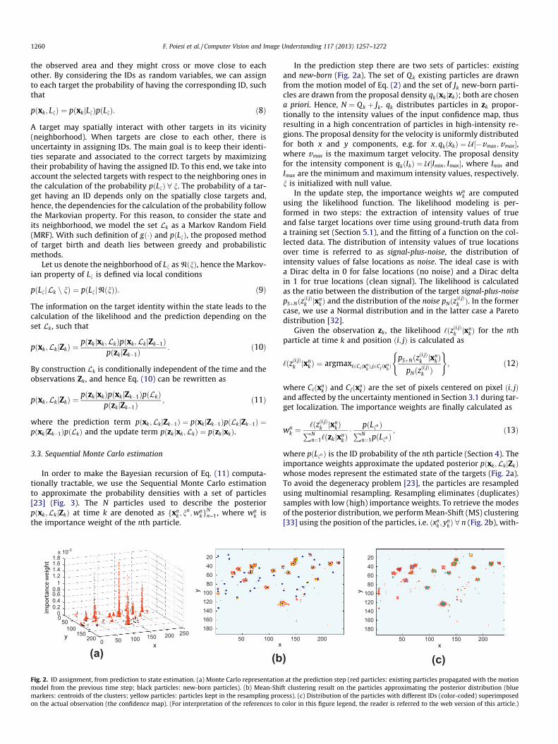
Fig. 2. ID assignment, from prediction to state estimation. (a) Monte Carlo representationmodel from the previous time step; black particles: new-born particles). (b) Mean-Shimarkers: centroids of the clusters; yellow particles: particles kept in the resampling procon the actual observation (the confidence map). (For interpretation of the references to
In the prediction step there are two sets of particles: existingand new-born (Fig. 2a). The set of Q k existing particles are drawnfrom the motion model of Eq. (2) and the set of Jk new-born parti-cles are drawn from the proposal density qkðxkjzkÞ; both are chosena priori. Hence, N ¼ Qk þ Jk. qk distributes particles in zk propor-tionally to the intensity values of the input confidence map, thusresulting in a high concentration of particles in high-intensity re-gions. The proposal density for the velocity is uniformly distributedfor both x and y components, e.g. for x; qkð _xkÞ ¼ U½�vmax;vmax�,where vmax is the maximum target velocity. The proposal densityfor the intensity component is qkðIkÞ ¼ U½Imin; Imax�, where Imin andImax are the minimum and maximum intensity values, respectively.n is initialized with null value.
In the update step, the importance weights wnk are computed
using the likelihood function. The likelihood modeling is per-formed in two steps: the extraction of intensity values of trueand false target locations over time using ground-truth data froma training set (Section 5.1), and the fitting of a function on the col-lected data. The distribution of intensity values of true locationsover time is referred to as signal-plus-noise, the distribution ofintensity values of false locations as noise. The ideal case is witha Dirac delta in 0 for false locations (no noise) and a Dirac deltain 1 for true locations (clean signal). The likelihood is calculatedas the ratio between the distribution of the target signal-plus-noisepSþNðz
ði;jÞk jxn
kÞ and the distribution of the noise pNðzði;jÞk Þ. In the former
case, we use a Normal distribution and in the latter case a Paretodistribution [32].
Given the observation zk, the likelihood ‘ðzði;jÞk jxnkÞ for the nth
particle at time k and position ði; jÞ is calculated as
‘ðzði;jÞk jxnkÞ ¼ argmaxi2Ciðxn
kÞ;j2Cjðxn
kÞ
pSþNðzði;jÞk jxn
kÞpNðz
ði;jÞk Þ
( ); ð12Þ
where CiðxnkÞ and Cjðxn
kÞ are the set of pixels centered on pixel ði; jÞand affected by the uncertainty mentioned in Section 3.1 during tar-get localization. The importance weights are finally calculated as
wnk ¼
‘ðzði;jÞk jxnkÞPN
n¼1‘ðzkjxnkÞ� pðLnn ÞPN
n¼1pðLnn Þ; ð13Þ
where pðLnn Þ is the ID probability of the nth particle (Section 4). Theimportance weights approximate the updated posterior pðxk;LkjZkÞwhose modes represent the estimated state of the targets (Fig. 2a).To avoid the degeneracy problem [23], the particles are resampledusing multinomial resampling. Resampling eliminates (duplicates)samples with low (high) importance weights. To retrieve the modesof the posterior distribution, we perform Mean-Shift (MS) clustering[33] using the position of the particles, i.e. ðxn
k ; ynkÞ 8 n (Fig. 2b), with-
150 200 50 100 150 200
20406080
100120140160180
) (c)at the prediction step (red particles: existing particles propagated with the motion
ft clustering result on the particles approximating the posterior distribution (blueess). (c) Distribution of the particles with different IDs (color-coded) superimposedcolor in this figure legend, the reader is referred to the web version of this article.)

Fig. 3. Block diagram of the proposed multi-target track-before-detect (MT-TBD). The filter receives as input the confidence map (zk) and draws the distribution of the targetstates using the Bayesian estimation with Monte Carlo approximation (particles). The weights of the particles are carried throughout the framework and used in the stateestimation stage to find the target locations (bxkjk). The states marked with the superscript � are generated after resampling. After the multi-target management stage, theweight distribution is uniform with respect to the number of the targets, Ok , at time k.
F. Poiesi et al. / Computer Vision and Image Understanding 117 (2013) 1257–1272 1261
out any prior knowledge on the number of clusters or their shape,and with a fixed cluster size.
Let us define the size of the cluster as kW and the set of clustersat time k as Wk ¼ fwrgr2Rk
, with wr the generic rth cluster and Rk
the set of cluster indexes. At this stage, the function gð�Þ introducedin Section 3.2 assigns a different ID to the particles belonging todifferent clusters at k ¼ 1. At k > 1, if a cluster contains onlynew-born particles, they are all initialized with a new ID. Other-wise, the ID is assigned to the new-born particles with a methodbased on Gaussian Mixture Model (GMM), as explained in the nextsection.
4. ID management with Markov Random Field
We address now the issues of managing multiple target identi-ties in the presence of interactions, target births and target deaths.We use the random variable Ln as a contribution to the posteriordistribution of Eq. (11) for penalizing particles belonging to a targetthat either mix with particles of other targets or move far from thetarget they represent. Being the target location spatially spread in akernel (i.e. Ciðxn
kÞ and CjðxnkÞ), particles belonging to a target are in
turn spread over the kernel (Fig. 2). Hence, when targets get closeto each other, particles are likely to mix (Fig. 4a), thus creating achallenging situation to manage in order to separately maintainthe identity of multiple targets.
To address this problem, let us characterize the set Lk and thejoint probability distribution pðLkÞ. Since Lk is a MRF, in order toconstruct the joint distribution of Lk considering the Markovianproperty of Eq. (9), we employ the Gibbs distribution [34],
pðLkÞ ¼1D
expfUðLkÞg; ð14Þ
where D is a normalization factor and Uð�Þ is the energy function
UðLkÞ ¼X
NðnÞ2NVNðnÞðLnÞ; ð15Þ
where N represents all the possible neighborhoods in the statespace and VNðnÞ is the potential function defined for the neighbor-hood NðnÞ. Since a potential function is defined on a single neigh-borhood, it ensures that it is possible to factorize the jointprobability such that the conditionally independent variables, forinstance from non-connected neighborhoods, do not contribute tothe same potential function.
Given a particle xnk , the probability of nn is pðLnn Þ and its neigh-
borhood NðnnÞ corresponds to the domain defined by the pixels af-fected by the blurring introduced during target localization, i.e.Ciðxn
kÞ and CjðxnkÞ (Eq. (12)).
The potential function of nn at time k associated to particle xnk is
calculated as
VNðnnÞðLnn Þ ¼ V 0NðnnÞðLnn Þ þ V 00NðnnÞðLnn Þ; ð16Þ
where V 0NðnnÞðLnn Þ evaluates the agreement of the ID of particle nwith respect to the IDs in NðnnÞ and V 00NðnnÞðLnn Þ evaluates the dis-tance between the ID of particle n and the center of mass of parti-cles with the same ID of particle n. We define
V 0NðnnÞðLnnÞ ¼ exp �a1ð1� dnkÞ
ink
q
� �; ð17Þ
where ink quantifies the agreement of the IDs and a1 regulates the
strength of the agreement. For instance, a high value of a1 leadsto a low probability of having an ID when a particle is surroundedby particles with different IDs, instead a low value of a1 keeps theprobability pðLnn Þ high when a particle is surrounded by particleswith different IDs. q normalizes the agreement value over the num-ber of particles in the neighborhood,
ink ¼ dNðnnÞ
k � aNðnnÞk ; ð18aÞ
q ¼ dNðnnÞk þ aNðnnÞ
k ; ð18bÞ
with dNðnnÞk as the number of different IDs and aNðnnÞ
k as the number ofsame IDs with respect to nn within the neighborhood NðnnÞ. dn
k is theDirac delta function that indicates if n is a new-born particle or not,
dnk ¼
1 if nn ¼ 00 if nn – 0
�: ð19Þ
In fact, if n is a new-born particle, then pðLnn Þ ¼ 1 with null ID. TheID will be assigned to the new-born particles at the multi-targetmanagement stage (Fig. 3). The potential V 00NðnnÞðLnn Þ is defined as
V 00NðnnÞðLnnÞ ¼ exp�ð1� dn
kÞðcnkÞ
4
2a2
( ); ð20Þ
where the rise ð�Þ4 and a2 are used to regulate the decreasing trendof the function. The higher a2, the higher the probability of havingan ID far from the group of particles with the same ID. cn
k is the nor-malized Euclidean distance from the center of mass and dn
k is de-fined as in Eq. (19).
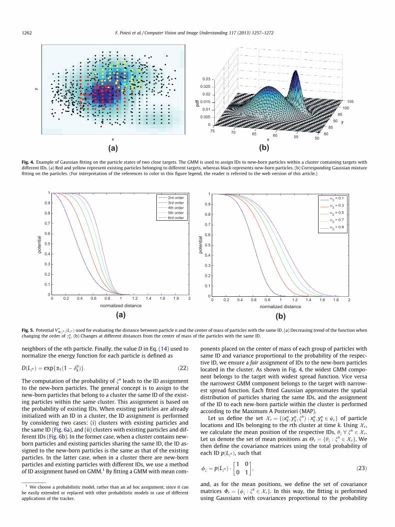
Fig. 5 shows the trend of the function with different parame-ters: the horizontal axis represents the variation of cn
k and the ver-tical axis represents V 00NðnnÞðLnn Þ as a function of cn
k . Fig. 5a shows thedecreasing trend of the potential function when changing the orderof cn
k , whereas Fig. 5b shows how the potential V 00NðnnÞðLnn Þ changesat different distances from the center of mass. The center of massis calculated by utilizing the geometric mean of the position ofthe particles with the same nn and the normalization is calculatedby taking into account the area of the pixels affected by the blur-ring introduced during target localization,
cnk ¼
14R
ffiffiffiffiffiffiffiffiffiffiffiffiffiffiffiffiffiffiffiffiffiffiffiffiffiffiffiffiffiffiffiffiffiffiffiffiffiffiffiffiffiffiffiffiffiffiffiffiffiffiffiffiffiffiffiffiffiffiffiffiffiffiffiffiffiffiffiffiffiffiffiffiffiffiffiffiffiffiffiffiffiffiffiffiffixn
k �
ffiffiffiffiffiffiffiffiffiffiffiffiffiYMm¼1
xmk
M
vuut0@ 1A2
þ ynk �
ffiffiffiffiffiffiffiffiffiffiffiffiffiYMm¼1
ymk
M
vuut0@ 1A2vuuut ; ð21Þ
where the normalizing factor 4R takes into account the 95% of thearea affected by the blurring and M ¼ jNðnnÞj is the number of
0 0.2 0.4 0.6 0.8 1 1.2 1.4 1.6 1.8 20
0.1
0.2
0.3
0.4
0.5
0.6
0.7
0.8
0.9
1
normalized distance
pote
ntia
l
2rd order3rd order4th order5th order6rd order
0 0.2 0.4 0.6 0.8 1 1.2 1.4 1.6 1.8 20
0.1
0.2
0.3
0.4
0.5
0.6
0.7
0.8
0.9
1
normalized distance
pote
ntia
l
2 = 0.1
2 = 0.3
2 = 0.5
2 = 0.7
2 = 0.9
(b)(a)
Fig. 5. Potential V 00Nðnn ÞðLnn Þ used for evaluating the distance between particle n and the center of mass of particles with the same ID. (a) Decreasing trend of the function whenchanging the order of cn
k . (b) Changes at different distances from the center of mass of the particles with the same ID.
8085
9095
100105
5055606570750
0.005
0.01
0.015
0.02
0.025
0.03
(b)(a)Fig. 4. Example of Gaussian fitting on the particle states of two close targets. The GMM is used to assign IDs to new-born particles within a cluster containing targets withdifferent IDs. (a) Red and yellow represent existing particles belonging to different targets, whereas black represents new-born particles. (b) Corresponding Gaussian mixturefitting on the particles. (For interpretation of the references to color in this figure legend, the reader is referred to the web version of this article.)
1262 F. Poiesi et al. / Computer Vision and Image Understanding 117 (2013) 1257–1272
neighbors of the nth particle. Finally, the value D in Eq. (14) used tonormalize the energy function for each particle is defined as
DðLnn Þ ¼ expfa1ð1� dnkÞg: ð22Þ
The computation of the probability of nn leads to the ID assignmentto the new-born particles. The general concept is to assign to thenew-born particles that belong to a cluster the same ID of the exist-ing particles within the same cluster. This assignment is based onthe probability of existing IDs. When existing particles are alreadyinitialized with an ID in a cluster, the ID assignment is performedby considering two cases: (i) clusters with existing particles andthe same ID (Fig. 6a), and (ii) clusters with existing particles and dif-ferent IDs (Fig. 6b). In the former case, when a cluster contains new-born particles and existing particles sharing the same ID, the ID as-signed to the new-born particles is the same as that of the existingparticles. In the latter case, when in a cluster there are new-bornparticles and existing particles with different IDs, we use a methodof ID assignment based on GMM.1 By fitting a GMM with mean com-
1 We choose a probabilistic model, rather than an ad hoc assignment, since it canbe easily extended or replaced with other probabilistic models in case of differentapplications of the tracker.
ponents placed on the center of mass of each group of particles withsame ID and variance proportional to the probability of the respec-tive ID, we ensure a fair assignment of IDs to the new-born particleslocated in the cluster. As shown in Fig. 4, the widest GMM compo-nent belongs to the target with widest spread function. Vice versathe narrowest GMM component belongs to the target with narrow-est spread function. Each fitted Gaussian approximates the spatialdistribution of particles sharing the same IDs, and the assignmentof the ID to each new-born particle within the cluster is performedaccording to the Maximum A Posteriori (MAP).
Let us define the set X r ¼ fðxnk ; y
nk ; n
nÞ : xnk ; y
nk 2 wrg of particle
locations and IDs belonging to the rth cluster at time k. Using X r ,we calculate the mean position of the respective IDs, hn 8 nn 2 X r .Let us denote the set of mean positions as Hr ¼ fhn : nn 2 X rg. Wethen define the covariance matrices using the total probability ofeach ID pðLnn Þ, such that
/n ¼ pðLnnÞ �1 00 1
� �; ð23Þ
and, as for the mean positions, we define the set of covariancematrices Ur ¼ f/n : nn 2 X rg. In this way, the fitting is performedusing Gaussians with covariances proportional to the probability

Fig. 6. Two sample cases of ID assignment to the new-born particles (black) using Mean-Shift clustering. (a) Cluster (green) containing existing particles with the same ID(red) that is assigned to all the new-born particles within the cluster. (b) Cluster (green) containing existing particles with different IDs (red and yellow) that are assigned tothe new-born particles within this cluster using a GMM approach (see text for details). (For interpretation of the references to color in this figure legend, the reader is referredto the web version of this article.)
F. Poiesi et al. / Computer Vision and Image Understanding 117 (2013) 1257–1272 1263
of the IDs within X r . Note that jHrj ¼ jUrj, where j � j is the cardinal-ity of a set. The GMM is defined as a weighted sum of Gaussian den-sities given by
f ðX rÞ ¼XjHr j
m¼1
pmNðX r jHr;m;Ur;mÞ; ð24Þ
where Hr;m and Ur;m denote the mth mean and covariance compo-nent of the corresponding sets, respectively, and each ID n 2 X r isassociated to each component m, i.e. n! m. The best fitting of themixture is performed through the Expectation–Maximizationalgorithm [35]. Fig. 4b shows an example of GMM fitting whentwo nearby targets are present. Once the GMM is fitted to theparticle locations, the affiliation of the new-born particles to thetargets is derived through the calculation of the MAP and the IDassignment is performed with respect to such information. Hence,8 ðxn
k ; ynk ; n
nÞ 2 X r with nn ¼ 0, the ID is assigned using the MAP
nn ¼ �n : �n! m0; m0 ¼ argmaxm¼1;...;jHr j pðmjðxnk ; y
nkÞÞ
� �; ð25Þ
where �n is the ID associated to the component with the highestprobability and
pðmjðxnk ; y
nkÞÞ ¼
pðmÞpððxnk ; y
nkÞjmÞ
pððxnk ; y
nkÞÞ
¼ pmNððxnk ; y
nkÞjHr;m;Ur;mÞPjHr j
m¼1pmNððxnk ; y
nkÞjHr;m;Ur;mÞ
: ð26Þ
The state estimate xkjk ¼ ðxkjk; ykjkÞ is finally calculated using theweighted sum of the particle positions on their relative weights,
xkjk;n ¼P
nwnk;n � ½xn
k;n ynk;n�
TPnwn
k;n
; ð27Þ
where the subscript n is used to indicate that the state estimate iscalculated among particles sharing the same ID.
Once the IDs are assigned, the resampling of the particleweights is performed for each cluster independently by assigningthe same number of particles to each cluster. Ideally, each clustercontains a single target, hence by resampling each cluster indepen-dently we ensure that all clusters/targets evolve over time with thesame number of particles.
5. Application to people tracking
In this section, we model the likelihood function and develop apostprocessing stage for people tracking applications. The postpro-cessing makes use of track duration in case of moving cameras, and
of background information and people appearance in case of staticcameras.
5.1. Likelihood modeling
The likelihood function (Eq. (12)) for MT-TBD is modeled usingautomatically generated confidence maps filtered by ground-truthinformation (Section 3.3). The intensity distribution of true loca-tions is referred to as signal-plus-noise, since manifold factorsmay affect the response of the target localization method, suchas objects with similar shape or color. The intensity distributionof false locations is referred to as noise. Ideally, a specific likelihoodfunction should be modeled for each scenario. However, in orderto demonstrate the flexibility of the proposed MT-TBD in differentscenarios and for different targets, a single likelihood function isdefined and used throughout our experiments. In particular, wemodel the likelihood function using highly noisy data, such ashead locations obtained by Support Vector Machine (SVM) [36]and by using HOG features [25] in the TRECVID dataset. The distri-bution of head/non-head confidences is shown in Fig. 7a. Fig. 7bshows the fitted curves on the data for modeling the likelihoodfunction. The signal-plus-noise distribution is fitted by a Normaldistribution and the noise distribution by a Pareto distribution[32]. Since the exponential function goes quicker to zero thanthe Pareto function, the Pareto distribution is more suited for mod-eling the noise in Eq. (12) (at the denominator). In fact, very highvalues of likelihood for high values of observed intensities wouldlead to the divergence in the estimation of the posterior distribu-tion (Eq. (11)).
The final likelihood ratio (Eq. (12)) is calculated as
pSþNðzði;jÞk jxn
kÞpNðz
ði;jÞk Þ
¼ r2ffiffiffiffiffiffiffi2pp
r11þ 1
zði;jÞk
r2
!ð1þ11Þ
� exp�ðzði;jÞk � hði;jÞk ðxkÞÞ
2r21
; ð28Þ
where r1 is the standard deviation of the Normal distribution, andr2 and 1 are the scale and tail parameters of the Pareto distribution,respectively.
Fig. 8 shows the effect of the parameter variations on thenumerator and denominator of Eq. (28). When pNðz
ði;jÞk Þ quickly de-
creases to zero, i.e. small r2 and small 1, the likelihood ratio giveshigh values. Vice versa, when pNðz
ði;jÞk Þ slowly decreases to zero, i.e.
if r2 and 1 are large, the likelihood gets more biased on the value ofthe numerator.

0 0.5 1 1.5 2 2.5 3 3.5 4 4.5 50
0.005
0.01
0.015
0.02
0.025
0.03Raw data
intensity level
frequ
ency
NoiseSignal + Noise
0 0.5 1 1.5 2 2.5 3 3.5 4 4.5 50
0.005
0.01
0.015
0.02
0.025
0.03Fitted functions
intensity level
frequ
ency
NoiseSignal + Noise
(a) (b)Fig. 7. (a) Distribution of the signal-plus-noise (blue) and noise (red) extracted from real data represented by the head locations [25] on the TRECVID dataset. (b) Normaldistribution fitted on signal-plus-noise (blue) and Pareto distribution on noise (red). (For interpretation of the references to color in this figure legend, the reader is referred tothe web version of this article.)
1264 F. Poiesi et al. / Computer Vision and Image Understanding 117 (2013) 1257–1272
5.2. Data-driven postprocessing
We use a shifting temporal window of s frames overlapping ofone frame over time. The tracks within this temporal window arecollected into the set
Tsk ¼ fT
sK;n : n 2 Nk;K ¼ ½ks; ke�;K # ½k� sþ 1; k�g; ð29Þ
where TsK;n is the generic track with ID n within the interval
K ¼ Ksn ¼ ½ks; ke� and ks; ke are the starting and ending instants of
the track within the temporal window, respectively.Each track is defined as Ts
K;n ¼ fðxk;n; bk;nÞ : n 2 Nk; k 2 Ksng,
2
where the state estimate xk;n corresponds to the top-left corner ofthe bounding box and bk;n is the bounding box associated to the statexk;n retrieved using the scene calibration information. Note that thepostprocessing introduces a delay in the tracking output that is ana-lyzed in details in Section 6.5.
The postprocessing stage for multi-person tracking is dividedinto (i) track pruning to remove tracks with a score s less than 3within a temporal window s1 ¼ 25 frames, (ii) track fusion withina temporal window s2 ¼ s and directly proportional to s1, and (iii)track pruning to remove fused tracks with score less than s2=10 fora temporal window of s2.
For track pruning, let us consider a generic track Ts1K;n with gen-
eric ID n that exists within the temporal interval s1. A score ss1n is
assigned to each track, such that
ss1K;n ¼
Xk2Ks1
n
rðTs1k;nÞ; ð30Þ
where r : Rm ! f0;1g and m is a set of rules used to define the score.This leads to ss1
k;n being equal to the duration of a track (in frames) ifrðTs1
k;nÞ ¼ 18k 2 Ks1n , otherwise, if rðTs1
k;nÞ ¼ 0 for some k 2 Ks1n , the
score ss1k;n is smaller than the duration of the track. The same process
is performed into the temporal window s2.In case of moving cameras, the function rð�Þ only evaluates the
duration of the track in frames. In case of static cameras, the func-tion rð�Þ is modeled as a logic AND of two rules, r1ð�Þ and r2ð�Þ, ob-tained from a background subtraction step. Given BðTs1
k;nÞ, a patchwithin each bounding box from the difference image betweenthe current frame fkðTs1
k;nÞ and the background, we define
2 The conditional dependency on k of xkjk;n is omitted for simplicity in the notation.
r1ðTs1k;pÞ ¼
0 if lðBðTs1k;nÞÞ < T1
1 otherwise
(; ð31Þ
where lð�Þ calculates the mean pixel intensity and T1 ¼ 20—25depending on the contrast between targets and background, and
r2ðTs1k;pÞ ¼
0 if rðfkðTs1k;nÞÞ > T2
1 otherwise
(; ð32Þ
where rð�Þ calculates the standard deviation of the pixel intensitiesin gray level and T2 ¼ 5 to remove false positive tracks on flat sur-faces such as walls. For the specific case of head tracking, we definean additional rule, r3ð�Þ, to calculate the relative distance and sizebetween bounding boxes in order to remove false tracks originateddue to shoulders, when they are erroneously detected as heads.
We formulate the track fusion process as a re-identificationproblem. The last available position of a track, the velocity andthe color extracted from the upper-body patch [37] are used to findthe best match between the final position of a track and the initialposition of another track ahead in time.
Let us define the function jð�Þ that calculates the cost betweeneach track pair within the temporal window s2 : jðTs2
K;n;Ts2K;n0 Þ is the
affinity between track n and track n0;8 n0 2 Nk n n. Using the tempo-ral gap between two tracks and the last available position of T
s2K;n,
we predict the target position with a linear motion model. Theaffinity is thus calculated from the end point of a track (Ts2
ke ;n) to
the start point of another track (Ts2ks ;n
0 ), with ks > ke. The calculationof the affinities is based on the Euclidean distance between pre-dicted and current starting point, and the Bhattacharyya distanceof the image patch at ke and that at ks. The Munkres algorithm3
is then iteratively computed to associate all the possible track pairs.
6. Experiments and results
6.1. Datasets and algorithms
In this section, the proposed MT-TBD is tested as multi-persontracking on confidence maps generated by six person localizationalgorithms (see [38] for a complete survey on person localization).
3 http://csclab.murraystate.edu/bob.pilgrim/445/munkres.html. Last accessed:March 2012.

0 0.5 1 1.5 2 2.5 3 3.5 40
0.005
0.01
0.015
0.02
0.025
0.03
hk(i,j)
2=0.70, =0.50
1=0.10
1=0.40
1=0.80
1=1.20
0 0.5 1 1.5 2 2.5 3 3.5 40
0.005
0.01
0.015
0.02
0.025
0.03
hk(i,j)
1=0.40
2=0.05, =0.50
2=0.15, =0.50
2=0.25, =0.50
2=0.40, =0.50
0 0.5 1 1.5 2 2.5 3 3.5 40
0.005
0.01
0.015
0.02
0.025
0.03
hk(i,j)
1=0.40
2=0.25, =0.05
2=0.25, =0.50
2=0.25, =1.00
2=0.25, =1.50
(a) (b)
(c)Fig. 8. Variation of the parameters of the fitted distributions for the likelihood function (Eq. (28)): (a) r1, (b) r2, and (c) 1.
F. Poiesi et al. / Computer Vision and Image Understanding 117 (2013) 1257–1272 1265
In particular, we retrieve person locations using information of:full-body [25,29], head [25,10], full-body based on parts [39] andfull-body from multiple views [40]. We firstly use reliable confi-dence maps obtained (i) from head locations guided by the groundtruth and (ii) from multiple views of the same scene. Then, wecompare the proposed method with the state of the art by employ-ing automatically generated confidence maps on single-view.
The experiments are performed on one sport video, four surveil-lance videos and two videos obtained from a moving camera. Thefirst set of reliable confidence maps are extracted on 2400 framesof size 720� 576 pixels from Camera 1 of the London Gatwick air-port dataset4 that is recorded at 25 Hz. The confidence maps aregenerated as the output of a SVM trained with HOG features [25],where false positive confidences are removed using ground-truthinformation. Let us call this dataset TRECVID�HOG+GT. In additionto this, we perform tracking on two different cameras of a basketballscenario (APIDIS dataset5) composed of 800 frames of size 800� 600pixels and recorded at 25 Hz. Let us call them APIDISC1 and API-DISC2. Here, the reliable sets of confidence maps are obtained by amulti-layered homography method [40] that exploits the seven cam-
4 iLIDS, Home Office multiple camera tracking scenario definition (UK), 2008.5 http://www.apidis.org/Dataset/. Last accessed: March 2012.
eras available in the dataset. Results on TRECVID�HOG+GT, API-DISC1 and APIDISC2 are reported in Section 6.4.
In Section 6.5, MT-TBD is then tested on automatically gener-ated confidence maps on single views. Firstly, we use the Town-Centre dataset6 composed of 4500 frames of size 1980� 1080pixels, recorded in Oxford (UK) town center at 25 Hz. For a fair com-parison with Benfold and Reid [10], we use the head locations pro-vided by the authors, which are generated using HOG features andSVM. As the provided person locations have already been threshol-ded, they are not in the form of intensity levels. For this reason,the input to MT-TBD is a confidence map with 2D Dirac delta in cor-respondence to each localized head. Moreover, we use the iLidsEasy7 dataset composed of 5220 frames of size 720� 576 pixels re-corded at the London Westminster subway station at 25 Hz, wherewe obtain person locations using an approach based on body-partsproposed by Felzenszwalb et al. [39]. Another localization methodbased on HOG features and SVM [25] is trained on head patches of24� 24 pixels, and applied to the London Gatwick airport datasetthat has the same specifications as above. Let us call this dataset
6 http://www.robots.ox.ac.uk/ActiveVision/Research/Projects/2009bbenfold_head-pose/project.html. Last accessed: March 2012.
7 http://www.eecs.qmul.ac.uk/�andrea/avss2007_d.html. Last accessed: March2012.
Table 2Summary of the datasets and person localization methods used for validation. Key: H:Head; B: Body; P-B: part-based.
Dataset Image size Localization method Bodypart
TRECVID�HOG+GT 720� 576 HOG + SVM [25] + GT HAPIDIS 800� 600 Multi-layer homography [40] BTownCentre 1920� 1080 Binary (HOG + SVM) [25] HiLids Easy 720� 576 HOG + SVM [39] B, P-BTRECVID 720� 576 HOG + SVM [25] HETH 640� 480 Binary (Edges + Weak
Classfier) [29]B
Table 3Parameters of the likelihood function (Eq. (28)) used in the experiments.
Dataset r1 r2 1
TRECVID�HOG+GT 0.70 0.10 0.60TRECVID 0.60 0.30 0.15iLids Easy 0.15 0.40 1.70APIDIS 0.70 0.16 0.25TownCentre 0.80 0.20 0.04ETH 0.80 0.22 0.05
1266 F. Poiesi et al. / Computer Vision and Image Understanding 117 (2013) 1257–1272
TRECVID to distinguish it from TRECVID�HOG+GT. Finally, we testMT-TBD on two videos from the ETH dataset8 recorded from a mov-ing camera at 13–14 Hz on outdoor scenarios, and composed of 353and 999 frames of size 640� 480 pixels. For a fair comparison withKuo et al. [9] and Yang and Nevatia [12] in this dataset, we employtheir full-body locations9 and, as for the TownCentre dataset, the in-put of MT-TBD for ETH is a confidence map with 2D Dirac delta sincethe provided locations have already been thresholded.
Table 2 summarizes the datasets and the localization methodsused for testing.
6.2. Parameters
This section describes the parameters used for MT-TBD. Simi-larly to Breitenstein et al. [20], some parameters are setexperimentally.
The choice of the maximum values of velocity, vmax, used topropagate the particles by the proposal density qkð�Þ (Section 3.3)depends on the frame resolution. Higher resolutions lead to highervalues of the maximum velocity. TRECVID and iLids Easy datasetshave the same frame resolution and, because they contain walkingpeople, the variance of motion is low. For this reason, we setq1 � 0:3 and vmax � 3. Similarly, the TownCentre dataset containswalking people, but the frame resolution is much higher (Table 2),thus leading to larger displacements on the image plane. Hence, weset q1 ¼ 4 and vmax ¼ 12. Since the ETH dataset is recorded with amoving camera and at low frame rate, the displacement for walk-ing people is larger than TRECVID and iLids Easy, and we set q1 ¼ 2and vmax ¼ 14. Finally, in the APIDIS dataset, we set q1 ¼ 3 andvmax ¼ 12 because people movements can be subject to suddenvariations.
The noise q2 associated to the intensity of the confidence map isthen chosen according to the specific confidence map given in in-put to MT-TBD. The confidence maps of TRECVID, iLids Easy andAPIDIS datasets are not thresholded, and we set Imin ¼ 1; Imax ¼ 3and q2 � 0:3 for all of them. In case of ETH and TownCentre data-sets, the confidence maps are thresholded (there is no variation ofintensity) and we set Imin ¼ Imax ¼ 2 with noise q2 ¼ 10�5.
The amount of blurring introduced in the target localizationprocess is modeled by R in Eq. (5): its value is dependent on theprecision of the person localization method and on the resolutionof the confidence map where higher resolution leads to a higherspread in intensity values. For example, R ¼ 1:3 for both TRECVIDand iLids Easy datasets that have the same person localizationmethod and the same frame resolution. On the contrary, in caseof the 2D Dirac delta confidence maps where blurring is absent,R ¼ 4 in order to have a similar spread of the particles over space.
The values of a1 and a2 for the MRF modeling (Section 4) de-pend on the desired strength level for maintaining the particles
8 http://www.vision.ee.ethz.ch/�aess/iccv2007/. Last accessed: March 2012.9 http://iris.usc.edu/people/yangbo/downloads.html. Last accessed: March 2012.
alive in case of mixing with different IDs. We use a1 ¼ 0:2 anda2 ¼ 0:02 for all the datasets.
The value of r1;r2 and 1 of Eq. (28) are provided in Table 3. Thevalues of r1 used in TRECVID�HOG+GT and TRECVID datasets aresimilar because the same person localization method is used inboth datasets, while the variation of r2 and 1 is due to the employ-ment of the ground-truth information in TRECVID�HOG+GT. Sincein TRECVID�HOG+GT, the noise due to false localizations is absent,we set r2 and 1 such that the numerator (signal-plus-noise) of thelikelihood function is predominant on the denominator (noise).Vice versa, in case of TRECVID, the confidence maps are more noisy,and r2 and 1 are set in order to take into account also the contri-bution of the denominator. The person localization method usedin iLids Easy [39] provides a more stable signal-plus-noise com-pared to the method used in TRECVID, thus leading to a smallervariance of the confidence values and hence to a smaller r1. How-ever, the noise is still high and r2 is set as for TRECVID. The value of1 is large, in order to avoid the divergence of the likelihood func-tion in case of large confidence values. For APIDIS, TownCentreand ETH datasets the confidence maps are provided as 2D Diracdelta functions and this justifies the similarity of r1 and r2 values.The parameters are chosen such that the likelihood function doesnot diverge. Unlike TownCentre and ETH datasets where the 2DDirac deltas are binary, in APIDIS the 2D Dirac deltas representconfidence values and, similarly to the iLids Easy, we keep the va-lue of 1 large in order to avoid the divergence of the likelihoodfunction for large confidence values.
6.3. Evaluation procedure
Given a bounding box for each target along with the confidencemap at each time step, a true positive track is defined as the onehaving a bounding box overlapping at least 25% the ground-truthbox in case of heads as targets, and at least 50% in case of fullbodies as targets [10]. Let tp be the number of all the true positivetracks in a video sequence, fp all the false positive tracks, fn all thefalse negative tracks, IDS the number of all ID switches, and NG thenumber of ground-truth targets. Performance scores are obtainedby calculating the Multiple Object Tracking Accuracy (MOTA), theMultiple Object Tracking Precision (MOTP), Precision and Recall[41]. MOTA is calculated as
MOTA ¼ 1� ðNG � tpÞ þ fpþ IDSNG
; ð33Þ
and MOTP as
MOTP ¼ Ot
Nm; ð34Þ
where Ot quantifies the overlap between the tracked boundingboxes and the ground-truth bounding boxes, and Nm is the numberof ground-truth targets mapped with the tracking output for thewhole video sequence. Precision, P, is calculated as
P ¼ tptpþ fp
; ð35Þ
and Recall, R, as

F. Poiesi et al. / Computer Vision and Image Understanding 117 (2013) 1257–1272 1267
R ¼ tptpþ fn
: ð36Þ
The results on the ETH dataset are evaluated using the toolbox pro-vided by Li et al. [4].
6.4. Validation
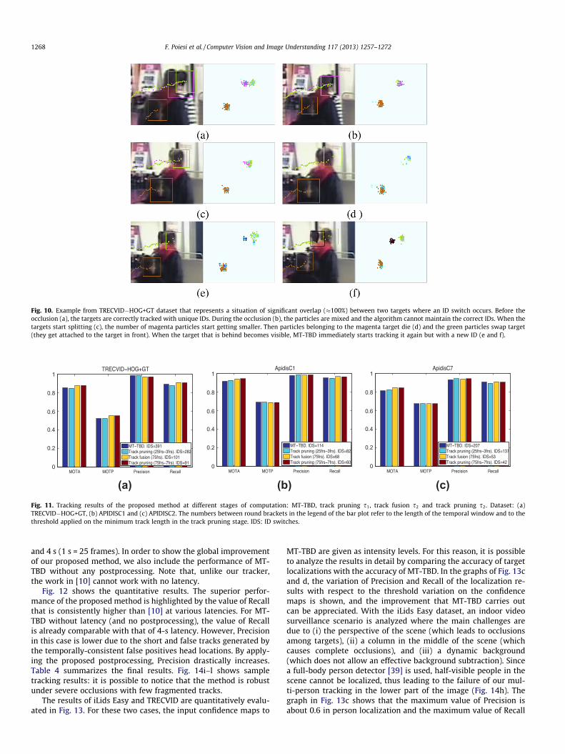
The validation for the robustness of the proposed method isperformed using the datasets TRECVID�HOG+GT, APIDISC1 andAPIDISC2, and in particular, we analyze the tracking results gener-ated by (i) MT-TBD without any postprocessing, (ii) track pruningon the tracks from MT-TBD, (iii) track fusion on the tracks fromthe previous track pruning, and (iv) track pruning on the tracksfrom the previous track fusion.
The analysis of the tracking results generated by MT-TBD with-out any postprocessing demonstrates the proposed filter, espe-cially in situations with close targets where the MRF modelinghelps avoiding particles of different targets to be mixed together.The first dataset we employ is the TRECVID�HOG+GT. In Fig. 9, asituation of a significant overlap (>50%) between two targets isshown. In Fig. 9a, all targets in the scene are correctly tracked. Sub-sequently, when two targets get closer (Fig. 9b), the target far apartfrom the camera gets almost completely occluded, however, sincethe confidence map still localizes the target, MT-TBD correctlytracks it. In Fig. 9c, when the targets are completely overlapped,the intensity levels on the confidence map appear as a single targetwith a large spread. Even if the tendency of mixing of particles withdifferent IDs is visible, the MRF modeling consistently assigns thecorrect ID to each particle. Fig. 9d–f finally show how the particlesremain associated to the correct target over time.
Fig. 10 shows an example of incorrect ID assignment leading toan ID switch generated by MT-TBD without any postprocessing. Inthis case, the confidence intensities are completely overlappedwith a mixing of IDs. Initially, two close targets move in the samedirection (Fig. 10a) and suddenly one target changes direction andbecomes completely occluded (Fig. 10b). Although both IDs remain
Fig. 9. Example from TRECVID�HOG+GT dataset that represents a situation of a signiocclusion occurs (a) the targets are correctly tracked with unique IDs. When the occlusocclusion (c), particles and IDs are mixed, but it is possible to notice that the mixing remamix (the red particles mix to the gray particles). When the split of targets occurs (e and f)references to color in this figure legend, the reader is referred to the web version of thi
alive for a few time steps, the particles with magenta ID die(Fig. 10d) and the green particles move on the visible target. Whenthe occluded target becomes visible again on the confidence map(Fig. 10e and f), MT-TBD immediately initializes a new track andcorrectly tracks the target in the following frames. Note that MT-TBD is not designed to reinitialize a target track with a previouslyexisting ID, hence a different ID is assigned to a target that disap-pears and reappears in a scene, thus leading to an ID switch(Section 6.3).
Quantitative results for MT-TBD and postprocessing are re-ported in Fig. 11a. After the first track pruning, Recall and MOTAare slightly decreased because the short tracks are removed dueto their low score. However, after track fusion has been applied,Recall reaches a higher value because short but reliable tracksare correctly fused. Lastly, by pruning the unreliable tracks gener-ated by the fusion stage, it is possible to keep the same value of Re-call while increasing Precision.
The second validation of MT-TBD and post-processing is pre-sented using APIDISC1 and APIDISC2 (Fig. 11). By analyzing the re-sults shown in Fig. 14a–d, we see the tracking succeeding in mostcases even while players are very close to each other. The mainchallenges here are the sudden movements of players. Recall is lar-ger than 90% in both datasets even if some of the tracks are lost(Fig. 14d). A possible solution for this problem is the use of mul-ti-dynamic model particle filters [23], which are able to performnonlinear filtering with switching of dynamic models.
6.5. Comparisons and discussion
As far as TownCentre dataset is concerned, we show how ourmethod outperforms the recent work by Benfold and Reid [10]by using the same observations for tracking. This scenario is fairlychallenging as it contains very close targets and the field-of-viewof the camera is very large, hence ID switches are likely to be fre-quent. For comparison, we present the results with the same la-tency used in [10] for postprocessing and, in particular, of 1, 2, 3,
ficant overlap (>50%) between two targets (red and gray color-codes). Before theion starts (b) particles start mixing but the IDs are still well-separated. During theins limited. When the targets start splitting (d), there is a tendency of the particles to, the particles are again well-separated with their own IDs. (For interpretation of thes article.)
0.8
1
0.6
0.4
0.2
0
0.8
1
0.6
0.4
0.2
0
0.8
1
0.6
0.4
0.2
0
(a) (b) (c)Fig. 11. Tracking results of the proposed method at different stages of computation: MT-TBD, track pruning s1, track fusion s2 and track pruning s2. Dataset: (a)TRECVID�HOG+GT, (b) APIDISC1 and (c) APIDISC2. The numbers between round brackets in the legend of the bar plot refer to the length of the temporal window and to thethreshold applied on the minimum track length in the track pruning stage. IDS: ID switches.
Fig. 10. Example from TRECVID�HOG+GT dataset that represents a situation of significant overlap (�100%) between two targets where an ID switch occurs. Before theocclusion (a), the targets are correctly tracked with unique IDs. During the occlusion (b), the particles are mixed and the algorithm cannot maintain the correct IDs. When thetargets start splitting (c), the number of magenta particles start getting smaller. Then particles belonging to the magenta target die (d) and the green particles swap target(they get attached to the target in front). When the target that is behind becomes visible, MT-TBD immediately starts tracking it again but with a new ID (e and f).
1268 F. Poiesi et al. / Computer Vision and Image Understanding 117 (2013) 1257–1272
and 4 s (1 s = 25 frames). In order to show the global improvementof our proposed method, we also include the performance of MT-TBD without any postprocessing. Note that, unlike our tracker,the work in [10] cannot work with no latency.
Fig. 12 shows the quantitative results. The superior perfor-mance of the proposed method is highlighted by the value of Recallthat is consistently higher than [10] at various latencies. For MT-TBD without latency (and no postprocessing), the value of Recallis already comparable with that of 4-s latency. However, Precisionin this case is lower due to the short and false tracks generated bythe temporally-consistent false positives head locations. By apply-ing the proposed postprocessing, Precision drastically increases.Table 4 summarizes the final results. Fig. 14i–l shows sampletracking results: it is possible to notice that the method is robustunder severe occlusions with few fragmented tracks.
The results of iLids Easy and TRECVID are quantitatively evalu-ated in Fig. 13. For these two cases, the input confidence maps to
MT-TBD are given as intensity levels. For this reason, it is possibleto analyze the results in detail by comparing the accuracy of targetlocalizations with the accuracy of MT-TBD. In the graphs of Fig. 13cand d, the variation of Precision and Recall of the localization re-sults with respect to the threshold variation on the confidencemaps is shown, and the improvement that MT-TBD carries outcan be appreciated. With the iLids Easy dataset, an indoor videosurveillance scenario is analyzed where the main challenges aredue to (i) the perspective of the scene (which leads to occlusionsamong targets), (ii) a column in the middle of the scene (whichcauses complete occlusions), and (iii) a dynamic background(which does not allow an effective background subtraction). Sincea full-body person detector [39] is used, half-visible people in thescene cannot be localized, thus leading to the failure of our mul-ti-person tracking in the lower part of the image (Fig. 14h). Thegraph in Fig. 13c shows that the maximum value of Precision isabout 0.6 in person localization and the maximum value of Recall
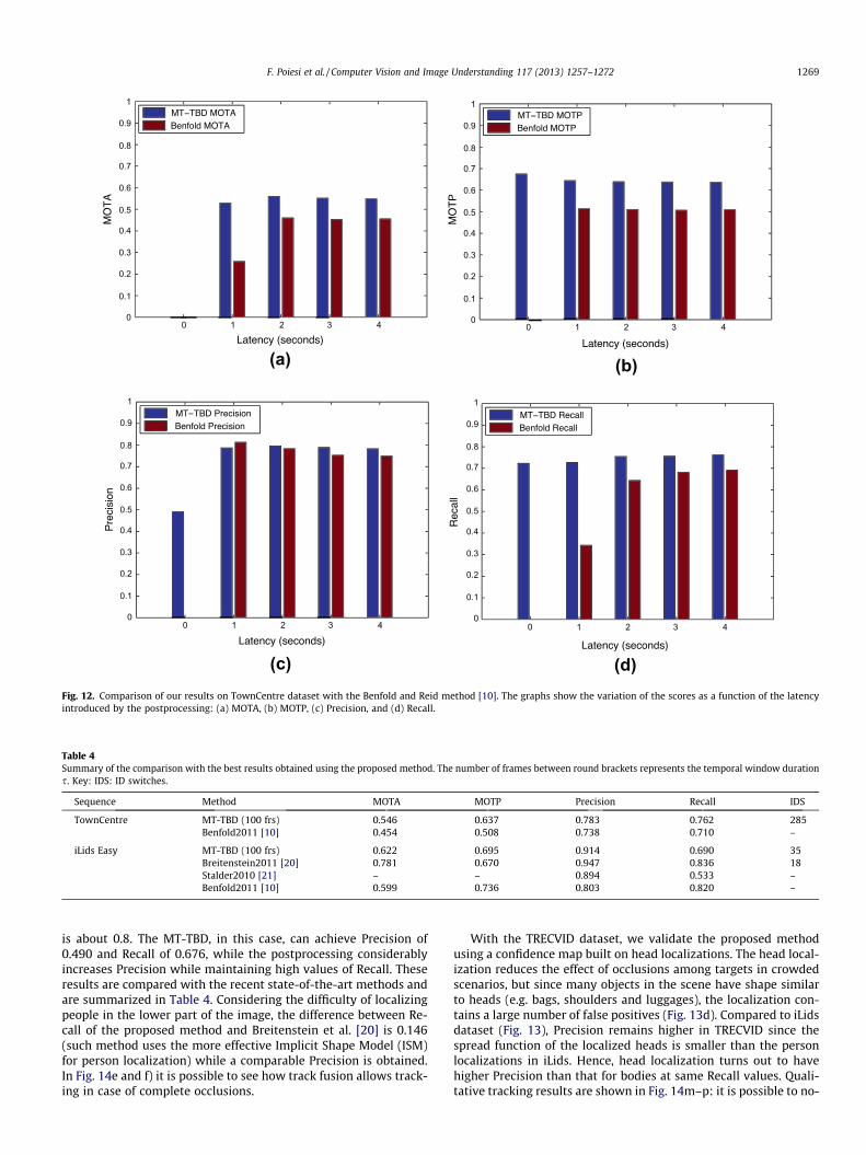
Table 4Summary of the comparison with the best results obtained using the proposed method. The number of frames between round brackets represents the temporal window durations. Key: IDS: ID switches.
Sequence Method MOTA MOTP Precision Recall IDS
TownCentre MT-TBD (100 frs) 0.546 0.637 0.783 0.762 285Benfold2011 [10] 0.454 0.508 0.738 0.710 –
iLids Easy MT-TBD (100 frs) 0.622 0.695 0.914 0.690 35Breitenstein2011 [20] 0.781 0.670 0.947 0.836 18Stalder2010 [21] – – 0.894 0.533 –Benfold2011 [10] 0.599 0.736 0.803 0.820 –
1
0.9
0.8
0.7
0.6
0.5
0.4
0.3
0.2
0.1
0
1
0.9
0.8
0.7
0.6
0.5
0.4
0.3
0.2
0.1
0
1
0.9
0.8
0.7
0.6
0.5
0.4
0.3
0.2
0.1
0
1
0.9
0.8
0.7
0.6
0.5
0.4
0.3
0.2
0.1
0
0 1 2 3 4 0 1 2 3 4
0 1 2 3 40 1 2 3 4
(a) (b)
(c) (d)Fig. 12. Comparison of our results on TownCentre dataset with the Benfold and Reid method [10]. The graphs show the variation of the scores as a function of the latencyintroduced by the postprocessing: (a) MOTA, (b) MOTP, (c) Precision, and (d) Recall.
F. Poiesi et al. / Computer Vision and Image Understanding 117 (2013) 1257–1272 1269
is about 0.8. The MT-TBD, in this case, can achieve Precision of0.490 and Recall of 0.676, while the postprocessing considerablyincreases Precision while maintaining high values of Recall. Theseresults are compared with the recent state-of-the-art methods andare summarized in Table 4. Considering the difficulty of localizingpeople in the lower part of the image, the difference between Re-call of the proposed method and Breitenstein et al. [20] is 0.146(such method uses the more effective Implicit Shape Model (ISM)for person localization) while a comparable Precision is obtained.In Fig. 14e and f) it is possible to see how track fusion allows track-ing in case of complete occlusions.
With the TRECVID dataset, we validate the proposed methodusing a confidence map built on head localizations. The head local-ization reduces the effect of occlusions among targets in crowdedscenarios, but since many objects in the scene have shape similarto heads (e.g. bags, shoulders and luggages), the localization con-tains a large number of false positives (Fig. 13d). Compared to iLidsdataset (Fig. 13), Precision remains higher in TRECVID since thespread function of the localized heads is smaller than the personlocalizations in iLids. Hence, head localization turns out to havehigher Precision than that for bodies at same Recall values. Quali-tative tracking results are shown in Fig. 14m–p: it is possible to no-

0.8
1
0.6
0.4
0.2
0
0.8
1
0.6
0.4
0.2
0
1
0.9
0.8
0.7
0.6
0.5
0.4
0.3
0.2
0.1
0
1
0.9
0.8
0.7
0.6
0.5
0.4
0.3
0.2
0.1
00.10 0.2 0.3 0.4 0.5 0.6 0.7 0.90.8 1 0.10 0.2 0.3 0.4 0.5 0.6 0.7 0.90.8 1
(c) (d)
(a) (b)
Fig. 13. Results of the proposed tracker and person localization methods obtained on iLids Easy and TRECVID datasets. (a and b) Bar plots of MOTA, MOTP, Precision andRecall values by varying the temporal window s used in the postprocessing. (c and d) Precision and Recall rates for the thresholded confidence map plotted along with thetracking scores that show tracking performance with respect to the input with varying threshold. The duration of the temporal window is indicated in frames (frs) within thelegend. IDS: ID switches.
1270 F. Poiesi et al. / Computer Vision and Image Understanding 117 (2013) 1257–1272
tice the long tracks belonging to the heads and the false positivetracks. The quantitative evaluation is given in Fig. 13b and d. Theimprovement of the tracker with respect to the confidence mapis shown in Fig. 13d, where Recall of 0.813 and Precision of 0.324are achieved. Then, the postprocessing phase improves the Preci-sion rate by around 20% at the cost of a slight decrease of Recall.
The last dataset we use for validation is ETH (Fig. 14q–t, wherefull-bodies [9] are represented as 2D Dirac deltas over the space.The experiments on this dataset are run with a latency of 3 s forthe proposed approach and compared with the recent offline meth-ods proposed by Kuo et al. [9] and Yang and Nevatia [12]. The per-formance comparison is shown in Table 5. The performance of theproposed method is comparable with the state-of-the-art methods,despite the diversity of the working modalities. Recall is at thesame level as the one obtained in Yang and Nevatia [12] and Pre-cision is slightly lower. Note that, since our method is not offline,some short tracks may not be fused together leading to a highernumber of fragmented tracks (second-last column in Table 5).
6.6. Computational cost
The overall complexity of MT-TBD with N particles has an upperbound of OðN logðNÞÞ operations. Specifically, for the motion mod-
el, the proposal distribution and the multinomial resampling (Sec-tion 3.1 and 3.3) the cost is OðNÞ, as these operations are sequentialon the number of particles. For the neighborhood search of Eq. (15),we give as input a set of spatially ordered particles at the cost ofOðN logðNÞÞ and we use a method based on binary search [42]whose cost is OðlogðNÞÞ. For the Mean-Shift clustering, the opera-tion is performed on the complete set of N particles with complex-ity OðN logðNÞÞ [43].
7. Conclusions
We presented a Bayesian method for multi-object trackingbased on track-before-detect, which utilizes a Markov Random Fieldapplied on the particles to perform tracking of unknown and largenumber of targets, and by probabilistically managing the ID assign-ment to avoid ID switches of close targets. The state estimate of atarget is performed via Mean-Shift clustering and supported byMixture of Gaussians in order to enable an accurate assignmentof IDs within each single cluster. The birth and death of the targetsat each iteration of the filter is modeled with a Markov RandomField. The computational complexity is proportional to the numberof particles only. The robustness of our algorithm was demon-strated by applying the method on sport and surveillance datasets
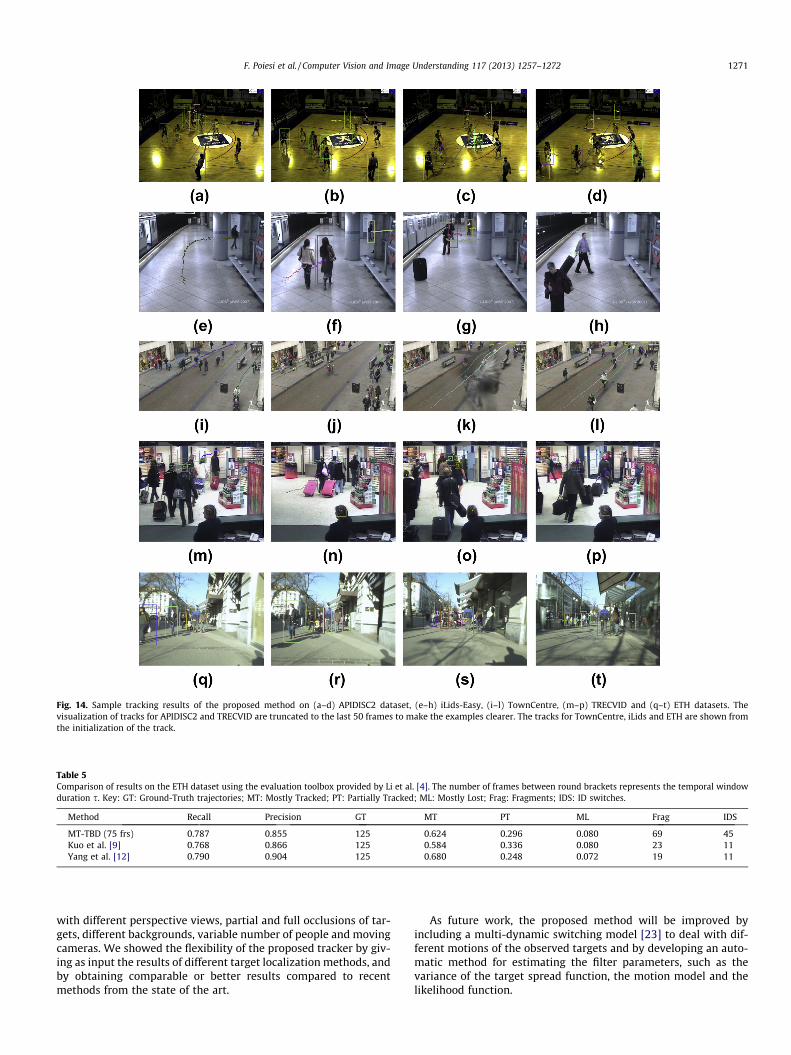
Table 5Comparison of results on the ETH dataset using the evaluation toolbox provided by Li et al. [4]. The number of frames between round brackets represents the temporal windowduration s. Key: GT: Ground-Truth trajectories; MT: Mostly Tracked; PT: Partially Tracked; ML: Mostly Lost; Frag: Fragments; IDS: ID switches.
Method Recall Precision GT MT PT ML Frag IDS
MT-TBD (75 frs) 0.787 0.855 125 0.624 0.296 0.080 69 45Kuo et al. [9] 0.768 0.866 125 0.584 0.336 0.080 23 11Yang et al. [12] 0.790 0.904 125 0.680 0.248 0.072 19 11
Fig. 14. Sample tracking results of the proposed method on (a–d) APIDISC2 dataset, (e–h) iLids-Easy, (i–l) TownCentre, (m–p) TRECVID and (q–t) ETH datasets. Thevisualization of tracks for APIDISC2 and TRECVID are truncated to the last 50 frames to make the examples clearer. The tracks for TownCentre, iLids and ETH are shown fromthe initialization of the track.
F. Poiesi et al. / Computer Vision and Image Understanding 117 (2013) 1257–1272 1271
with different perspective views, partial and full occlusions of tar-gets, different backgrounds, variable number of people and movingcameras. We showed the flexibility of the proposed tracker by giv-ing as input the results of different target localization methods, andby obtaining comparable or better results compared to recentmethods from the state of the art.
As future work, the proposed method will be improved byincluding a multi-dynamic switching model [23] to deal with dif-ferent motions of the observed targets and by developing an auto-matic method for estimating the filter parameters, such as thevariance of the target spread function, the motion model and thelikelihood function.
1272 F. Poiesi et al. / Computer Vision and Image Understanding 117 (2013) 1257–1272
References
[1] A. Yilmaz, O. Javed, M. Shah, Object tracking: a survey, ACM Comput. Surv. 38(2006) 1–45.
[2] Y. Boers, J.N. Driessen, Multitarget particle filter track-before-detectapplications, IEE Proc. Radar, Sonar Navig. 151 (2004) 351–357.
[3] C. Huang, B. Wu, R. Nevatia, Robust object tracking by hierarchical associationof detection responses, in: Proc. of European Conference on Computer Vision,Marseille, France, 2008, pp. 788–801.
[4] Y. Li, C. Huang, R. Nevatia, Learning to associate: hybridboosted multi-targettracker for crowded scene, in: Proc. of IEEE Computer Vision and PatternRecognition, Miami, FL, USA, 2009, pp. 2953–2960.
[5] E. Maggio, A. Cavallaro, Learning scene context for multiple object tracking,IEEE Trans. Image Process. 18 (2009) 1873–1884.
[6] C. Kuo, C. Huang, R. Nevatia, Multi-target tracking by on-line learneddiscriminative appearance models, in: Proc. of IEEE Computer Vision andPattern Recognition, San Francisco, CA, USA, 2010, pp. 685–692.
[7] M. Rodriguez, I. Laptev, J. Sivic, J. Audibert, Density-aware person detection andtracking in crowds, in: Proc. of IEEE International Conference on ComputerVision, Barcelona, Spain, 2011, pp. 2423–2430.
[8] B. Yang, C. Huang, R. Nevatia, Learning affinities and dependencies for multi-target tracking using a CRF models, in: Proc. of IEEE Computer Vision andPattern Recognition, Colorado Springs, USA, 2011, pp. 1233–1240.
[9] C. Kuo, R. Nevatia, How does person identity recognition help multi-persontracking?, in: Proc. of IEEE Computer Vision and Pattern Recognition, ColoradoSprings, USA, 2011, pp. 1217–1224.
[10] B. Benfold, I.D. Reid, Stable multi-target tracking in real-time surveillancevideo, in: Proc. of IEEE Computer Vision and Pattern Recognition, ColoradoSprings, USA, 2011, pp. 3457–3464.
[11] B. Yang, R. Nevatia, Multi-target tracking by online learning of non-linearmotion patterns and robust appearance model, in: Proc. of IEEE ComputerVision and Pattern Recognition, Providence, Rhode Island, USA, 2012, pp.1918–1925.
[12] B. Yang, R. Nevatia, An online learned CRF model for multi-target tracking, in:Proc. of Computer Vision and Pattern Recognition, Providence, Rhode Island,USA, 2012, pp. 2034–2041.
[13] Z. Khan, T. Balch, F. Dellaert, MCMC data association and sparse factorizationupdating for real time multitarget tracking with merged and multiplemeasurements, IEEE Trans. Pattern Anal. Mach. Intell. 28 (2006) 1960–1972.
[14] J. Czyz, B. Ristic, B. Macq, A particle filter for joint detection and tracking ofcolor objects, Image Vision Comput. 25 (2007) 1271–1281.
[15] J. Xing, H. Ai, S. Lao, Multi-object tracking through occlusions by local trackletsfiltering and global tracklets association with detection responses, in: Proc. ofIEEE Computer Vision and Pattern Recognition, Miami, FL, USA, 2009, pp.1200–1207.
[16] I. Ali, M.N. Dailey, Multiple human tracking in high-density crowds, in: Proc ofConference on Advanced Concepts for Intelligent Vision Systems, Bordeaux,France, 2009, pp. 540–549.
[17] M. Yang, F. Lv, W. Xu, Y. Gong, Detection driven adaptive multi-cue integrationfor multiple human tracking, in: Proc. of IEEE International Conference onComputer Vision, Kyoto, Japan, 2009, pp. 1554–1561.
[18] B.-N. Vo, B.-T. Vo, N.-T. Pham, D. Suter, Joint detection and estimation ofmultiple objects from image observations, IEEE Trans. Signal Process. 58(2010) 5129–5241.
[19] H. Tong, H. Zhang, H. Meng, X. Wang, Multitarget tracking before detection viaprobability hypothesis density filter, in: Int. Conference on Electrical andControl Engineering, Wuhan, China, 2010, pp. 1332–1335.
[20] M.D. Breitenstein, F. Reichlin, B. Leibe, E. Koller-Meier, L. Van Gool, Onlinemultiperson tracking-by-detection from a single, uncalibrated camera, IEEETrans. Pattern Anal. Mach. Intell. 33 (2011) 1820–1833.
[21] S. Stalder, H. Grabner, L. Van Gool, Cascaded confidence filtering for improvedtracking-by-detection, in: Proc. of European Conference on Computer Vision,Crete, Greece, 2010, pp. 369–382.
[22] T. De Laet, H. Bruyninckx, J. De Schutter, Shape-based online multitargettracking and detection for targets causing multiple measurements: variationalbayesian clustering and lossless data association, IEEE Trans. Pattern Anal.Mach. Intell. 33 (2011) 2477–2491.
[23] B. Ristic, S. Arulampalam, N. Gordon, Beyond the Kalman Filter: Particle Filtersfor Tracking Applications, Artech House, Boston, 2004.
[24] S. Buzzi, M. Lops, L. Venturino, M. Ferri, Track-before-detect procedures in amulti-target environment, IEEE Trans. Aerosp. Electr. Syst. 44 (2008) 1135–1150.
[25] N. Dalal, B. Triggs, Histograms of oriented gradients for human detection, in:Proc. of IEEE Computer Vision and Pattern Recognition, San Diego, CA, USA,2005, pp. 886–893.
[26] S. Ali, M. Shah, Floor fields for tracking in high density crowd scenes, in: Proc.of European Conference on Computer Vision, Marseille, France, 2008, pp. 1–14.
[27] M. Rodriguez, S. Ali, T. Kanade, Tracking in unstructured crowded scenes, in:Proc. of IEEE International Conference on Computer Vision, Kyoto, Japan, 2009,pp. 1389–1396.
[28] D. Reid, An algorithm for tracking multiple targets, IEEE Trans. Autom. Control24 (1979) 843–854.
[29] B. Wu, R. Nevatia, Detection and tracking of multiple, partially occludedhumans by bayesian combination of edgelet based part detectors, Int. J.Comput. Vision 75 (2007) 247–266.
[30] W. Ng, J. Li, S. Godsill, J. Vermaak, A review of recent results in multiple targettracking, in: Proc. of Image and Signal Processing and Analysis, Trieste, Italy,2005, pp. 40–45.
[31] R. Hoseinnezhad, B.-N. Vo, D. Suter, B.-T. Vo, Multi-object filtering from imagesequence without detections, in: Proc. of International Conference on Acoustic,Speech and Signal Processing, Dallas, Texas, USA, 2010, pp. 1154–1157.
[32] J.R.M. Hosking, J.R. Wallis, Parameter and quantile estimation for thegeneralized Pareto distribution, Technometrics 29 (1987) 339–349.
[33] D. Comaniciu, P. Meer, Distribution free decomposition of multivariate data,IEEE Trans. Pattern Anal. Mach. Intell. 2 (1999) 22–30.
[34] R. Kindermann, J.L. Snell, Markov Random Fields and Their Applications,American Mathematical Society, Providence, Rhode Island, 2000.
[35] R. Hogg, J. McKean, A. Craig, Introduction to Mathematical Statistics, UpperSaddle River, NJ, 2005.
[36] R. Duda, P. Hart, D. Stork, Pattern Classification, John Wiley & Sons, Singapore,2001.
[37] R. Mazzon, S.F. Tahir, A. Cavallaro, Person re-identification in crowd, PatternRecogn. Lett. 33 (2012) 1828–1837.
[38] P. Dollar, C. Wojek, B. Schiele, P. Perona, Pedestrian detection: an evaluation ofthe state of the art, IEEE Trans. Pattern Anal. Mach. Intell. 34 (2012) 743–761.
[39] P.F. Felzenszwalb, R.B. Girshick, D. McAllester, D. Ramanan, Object detectionwith discriminatively trained part based models, IEEE Trans. Pattern Anal.Mach. Intell. 32 (2010) 1627–1645.
[40] R. Eshel, Y. Moses, Homography based multiple camera detection and trackingof people in a dense crowd, in: Proc. of IEEE Computer Vision and PatternRecognition, Anchorage, AK, US, 2008, pp. 1–8.
[41] K. Bernardin, R. Stiefelhagen, Evaluating multiple object tracking performance:the CLEAR MOT metrics, EURASIP J. Image Video Process. 2008 (2008) 246–309.
[42] T. Cormen, C. Leiserson, R. Rivest, C. Stein, Introduction to Algorithms, MITpress, Cambridge, MA, 1990.
[43] B. Georgescu, I. Shimshoni, P. Meer, Mean-Shift based clustering in highdimensions: a texture classification example, in: Proc. of IEEE InternationalConference on Computer Vision, Beijing, China, 2003, pp. 456–463.