University of Calgary

PRISM: University of Calgary's Digital Repository

Graduate Studies The Vault: Electronic Theses and Dissertations

2015-09-29

Multi-parametric Programming for Microgrid

Operational Scheduling

Umeozor, Eva Chinedu

Umeozor, E. C. (2015). Multi-parametric Programming for Microgrid Operational Scheduling

(Unpublished master's thesis). University of Calgary, Calgary, AB. doi:10.11575/PRISM/27031

http://hdl.handle.net/11023/2544

master thesis

University of Calgary graduate students retain copyright ownership and moral rights for their

thesis. You may use this material in any way that is permitted by the Copyright Act or through

licensing that has been assigned to the document. For uses that are not allowable under

copyright legislation or licensing, you are required to seek permission.

Downloaded from PRISM: https://prism.ucalgary.ca

UNIVERSITY OF CALGARY

Multi-parametric Programming for Microgrid Operational Scheduling

by

Eva Chinedu Umeozor

A THESIS

SUBMITTED TO THE FACULTY OF GRADUATE STUDIES

IN PARTIAL FULFILMENT OF THE REQUIREMENTS FOR THE

DEGREE OF MASTERS OF SCIENCE

GRADUATE PROGRAM IN CHEMICAL ENGINEERING

CALGARY, ALBERTA

September 2015

© Eva Chinedu Umeozor 2015

ii

Abstract

This study presents a multi-parametric programming (MPP) based approach for energy

management in microgrids. The algorithm creates operational strategies for efficient and

tractable coordination of distributed energy sources in a residential level microgrid. The

hybrid energy system comprises of renewable (solar photovoltaic and wind turbine),

conventional systems (microturbine and utility grid connection), and battery energy storage

system. The overall problem is formulated using multi-parametric mixed-integer linear

programming (mp-MILP) via parameterizations of the uncertain coordinates of the wind

and solar resources. This results in a bi-level optimization problem, where choice of the

parameterization scheme is made at the upper level while system operation decisions are

made at the lower level. The mp-MILP formulation leads to significant improvements in

uncertainty management, solution quality and computational burden; by easing

dependency on meteorological information and avoiding the multiple computational cycles

of the traditional online optimization techniques. Results evidence the feasibility and

effectiveness of MPP.

iii

Acknowledgements

The author would like to express his honest gratitude to his supervisor Dr. Milana

Trifkovic for her patience, continuous support, encouragement and supervision of this

thesis.

The author also expresses his appreciation to the members of the examining

committee for their valuable comments

The author wants to thank all members of the Trifkovic Group for their comments

regarding this work.

Suggestions and data provided by Bluewater Power are highly valued. Financial

support provided by the Natural Sciences and Engineering Research Council of Canada

(NSERC) is greatly appreciated by the author.

Finally, the author thanks the financial support provided by the department of

Chemical and Petroleum Engineering for completing the present study.

iv

Dedication

This thesis is dedicated to my mother, Nneka (“Mother is Supreme”).

v

Table of Contents

Approval Page ..................................................................................................................... ii

Abstract ............................................................................................................................... ii

Acknowledgements ............................................................................................................ iii Dedication .......................................................................................................................... iv Table of Contents .................................................................................................................v List of Tables ..................................................................................................................... vi List of Figures and Illustrations ........................................................................................ vii

List of Symbols, Abbreviations and Nomenclature ........................................................... ix

INTRODUCTION ..................................................................................1 1.1 Background ................................................................................................................1

1.2 Problem Statement and Thesis Contributions ............................................................5

LITERATURE REVIEW ......................................................................9 2.1 Fundamentals of Optimization and Control ...............................................................9

2.1.1 Optimization ......................................................................................................9 2.1.2 Control .............................................................................................................13

2.2 Microgrid Energy Management ...............................................................................16 2.3 Microgrid Component Modelling ............................................................................34

2.3.1 Solar Photovoltaic Model ................................................................................34

2.3.2 Wind Turbine Model .......................................................................................35 2.3.3 Battery Energy Storage Model ........................................................................36

2.3.4 Microturbine Model .........................................................................................38

2.3.5 Electricity Pricing and Load Demand Model ..................................................39

2.3.6 Uncertainty Modelling in Renewable Energy Systems ...................................43

METHODOLOGY ..........................................................................45

3.1 Multi-parametric Programming ...............................................................................45 3.2 Problem Formulation ...............................................................................................49

RESULTS AND DISCUSSION ........................................................58 4.1 Discussion of Results ...............................................................................................58

CONCLUSIONS AND RECOMMENDATIONS ..............................75 5.1 Conclusions ..............................................................................................................75 5.2 Recommendations ....................................................................................................77

BIBLIOGRAPHY ..................................................................................79

APPENDICES ...................................................................................................................87

vi

List of Tables

Table 3-1: Cost characteristics of the microgrid components .......................................... 55

Table 3-2: Simulation parameters .................................................................................... 56

Table 4-1: Comparing the cost of running a microgrid and that of relying on the utility.

................................................................................................................................... 74

vii

List of Figures and Illustrations

Figure 1-1: Left – world total final consumption by fuel in million tonnes of oil

equivalent (Mtoe) [1]. Right – global CO2 emissions by region in billion tonnes

(Gt) [2]. ....................................................................................................................... 2

Figure 1-2: Comparing the present centralised operation and control with the future

distributed generation with bidirectional communications [5]. .................................. 4

Figure 1-3: Microgrid system components and their specifications based on the

existing system in Lambton College, Ontario. System information includes; real-

time electricity pricing, weather data and battery state of charge. The EMS

integrates the units through a collective economical operation problem

formulation. ................................................................................................................. 6

Figure 1-4: Energy management in a microgrid via bidirectional communication

between the energy system components and the optimizer. ....................................... 8

Figure 2-1: Convex (right) and non-convex (left) regions. .............................................. 11

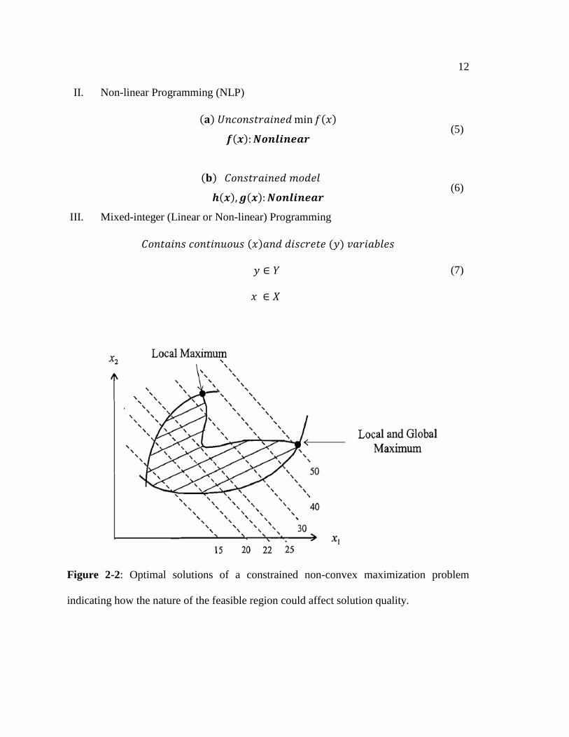
Figure 2-2: Optimal solutions of a constrained non-convex maximization problem

indicating how the nature of the feasible region could affect solution quality. ........ 12

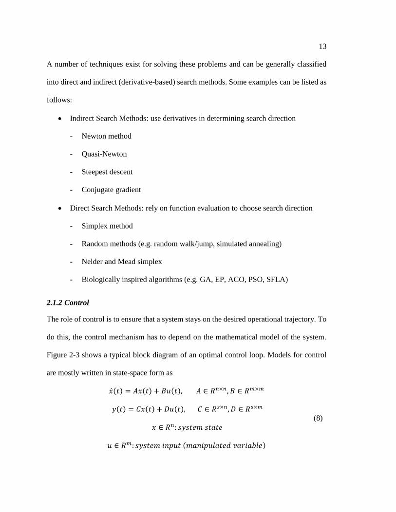
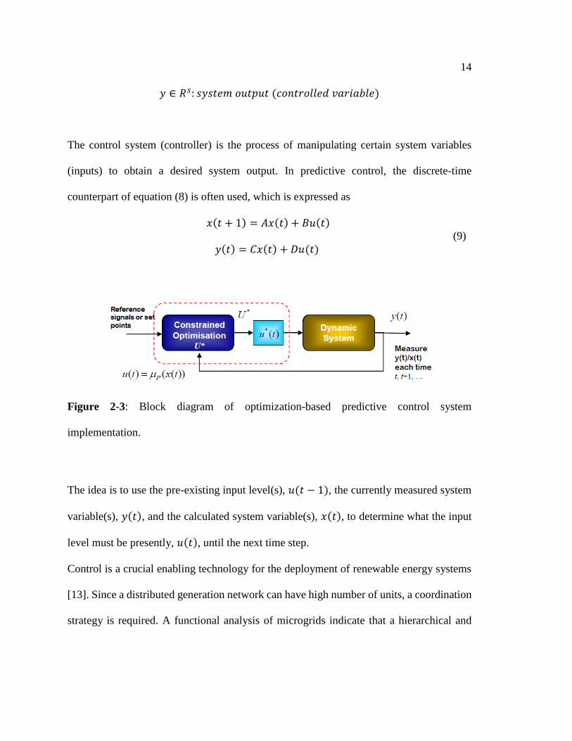
Figure 2-3: Block diagram of optimization-based predictive control system

implementation. ........................................................................................................ 14

Figure 2-4: Power systems management and control hierarchies. ................................... 16

Figure 2-5: Model predictive control scheme block diagram .......................................... 20

Figure 2-6: Model predictive control scheme implementation [73]. ............................... 21

Figure 2-7: Load shifting curve from peak to valley [101]. ............................................. 40

Figure 2-8: Load shifting curve from flat to valley [101]. ............................................... 40

Figure 2-9: Load shifting curve from peak to flat [101]. ................................................. 41

Figure 3-1: Solar and wind power scenarios showing critical nodes in green ................. 50

Figure 3-2: Scenario mesh of solar and wind power production showing the

parameterizations in green and realized scenarios in red. ......................................... 51

Figure 4-1: Electricity price profile for Ontario over a seven year period (courtesy of

Bluewater Power Corporation). The negative prices occur when power producers

are willing to pay in order to feed power into the network. ...................................... 59

Figure 4-2: Expected and realized renewables harvesting scenarios. The expected

scenarios are developed from a coarse day-ahead forecast while the realized

viii

variations are the actual observations on the day in Ontario. Highlighted numbers

(red) indicate the sequence of variation of solar and wind resources. The 20th

through 24th realized scenarios fall on the same node. ............................................. 61

Figure 4-3: Effect of resolution factor on the average net cost for a 24hrs operational

schedule. .................................................................................................................... 62

Figure 4-4: Effect of resolution factor on the computational time for a 24hrs

operational schedule. ................................................................................................. 62

Figure 4-5: Realistic pricing schemes based on Ontario data. FITs is for roof-top solar

while FITw is for onshore wind power. TOU is the time-of-use billing

arrangement from Bluewater Power. ETS is the real-time dynamic price. .............. 63

Figure 4-6: (a) – Power supply under FIT and ETS schemes (with real dynamic

electricity price); (b) – The local load demand profile. ............................................ 65

Figure 4-7: Battery state of charge profiles under the dynamic spot market and fixed

contract pricing schemes. .......................................................................................... 66

Figure 4-8: Effect of pricing dynamics on battery state of charge; considering the actual

pricing (P*) and hypothetical pricing (P**) scenarios under the ETS system: (a) –

state of charge for the fixed capacity storage; (b) – state of charge for the estimated

capacity storage; (c) – dynamic real-time low and high electricity price scenarios.

................................................................................................................................... 68

Figure 4-9: Microgrid and the utility grid interaction depicting how electricity is sold

under each pricing scheme and storage model: (a) – power sold to utility under a

fixed maximum state of charge limit; (b) – power sold to utility under a variable

maximum state of charge limit. ................................................................................ 70

Figure 4-10: Microgrid and the main grid interaction displaying how power is bought

from the utility grid under each pricing scheme and storage model: (a) – power

purchased from utility under a fixed maximum state of charge limit; (b) – power

purchased from utility under a variable maximum state of charge limit. ................. 71

Figure 4-11: Microturbine activation profile under the pricing schemes and storage

models. The microturbine remains shutdown for the low price regime ETS and the

FIT program. (a) – microturbine activation state under the fixed maximum state

of charge limit. (b) – microturbine activation state under the variable maximum

state of charge limit. .................................................................................................. 72

Figure 4-12: Comparison of the net operating and maintenance cost of the microgrid

under various pricing scenarios and storage models, and the cost of purchasing all

power demands from the utility grid using the TOU pricing scheme. ...................... 73

ix

List of Symbols, Abbreviations and Nomenclature

Symbols Definition

𝑤, 𝑠, 𝑔, 𝑢, 𝑏 Wind turbine, Solar PV, Microturbine, Utility, Battery

𝑒𝑝 Electricity price

𝑃𝑏0 Charging power of battery

𝑃𝑏1 Discharging power of battery

𝐸𝑏0 Charged energy of battery

𝐸𝑏1 Discharged energy of battery

𝐸𝜽𝑘 Set of realized operational net costs

𝑄 Expected net cost of microgrid operation

𝑍 Realized net cost of microgrid operation

𝐷𝑉𝑖 Depreciable value of component 𝑖

𝜃𝑤 Parameterized wind power

𝜃𝑠 Parameterized solar power

𝑣 Wind speed

𝐻 Insolation

𝑚𝑠𝑐 Emissions cost

𝑀𝑖 Net cost of microgrid system component 𝑖

𝑐 Microgrid component O&M cost

ℎ𝑖 Depreciation of system component 𝑖

𝐿 Dynamic load demand

𝑘 Discrete time

𝑙𝑡𝑖 Lifetime of component 𝑖

x

𝑦𝑖 Activation state of system component 𝑖

𝑃𝑢𝑏 Power bought from the utility grid

𝑃𝑢𝑠 Power sold to the utility grid

𝑃𝑔 Microturbine power rating

𝐶𝑏𝑎𝑡 Battery storage capacity

𝑆𝑂𝐶 Battery state of charge

Abbreviation Nomenclature

ACO Ant Colony Optimization

PSO Particle Swarm Optimization

SLFA Shuffled Leap Frog Algorithm

GA Genetic Algorithm

EP Evolutionary Programming

DSO Distributed System Operator

FIT Feed-In Tariff

ETS Real-time Energy Trading System pricing

TOU Time of Use pricing

MPC Model Predictive Control

MPP Multi-Parametric Programming

RHO Receding/Rolling Horizon Optimization

SA Simulated Annealing

FA Firefly Algorithm

RH Rolling Horizon

PEM Point Estimate Method

1

Introduction

This chapter overviews historical and projected energy demand and supply trends, in

addition to the social, technological and environmental factors that are relevant to the study.

In section 1.2, the research problem is described and the solution approach is presented.

1.1 Background

Energy is life to both current and future global economy. With the United Nations’ estimate

of world population growth at 74 million people per year, energy demand will continue to

increase with human population growth and technological advancement. The International

Energy Agency predicts that global energy demand will grow by 37% of the 2012 value,

by the year 2040 [1]. Figure 1-1 is the past global energy consumption and carbon

emissions trends, indicating an overall increasing tendency. Therefore, concerns about

climate change, cost of energy, efficiency and reliability of energy systems necessitate

reshaping/upgrading of the global energy landscape to cope with present and anticipated

environmental, economic and social needs. In 2013, global CO2 emissions – a major

greenhouse gas – stood at 35.3 billion tonnes (Gt), which is 0.7 Gt higher than the 2012

level [2]. This moderate increase of 2% - as against average yearly growth rate of 3.8%

since 20031 - is a continuation of recent trends in the slowdown of yearly emissions growth,

which has been attributed to developments in the electric power sector [2, 3]. However, of

the calculated total energy demand in 2012 of 104426 TWh, electricity accounted for only

18.1% [1]. If global carbon emissions target is to be met in the future, more avenues to

emissions reduction/elimination need to be exploited. Unfortunately, optimal energy

1 Excluding the 2008-2009 recession years 2. Olivier, J.G.J., et al., Trends in global CO2 emissions,

P.a.E.C.s.J.R. Centre, Editor. 2014: The Hague.

2

conservation and efficiency techniques for fossil fuel based systems can neither guarantee

energy sufficiency in the future nor meet the environmental conservation needs [3, 4].

Therefore, finding suitable renewable and clean energy sources for the future is one of

society’s daunting challenges.

Figure 1-1: Left – world total final consumption by fuel in million tonnes of oil equivalent

(Mtoe) [1]. Right – global CO2 emissions by region in billion tonnes (Gt) [2].

Since most of the world’s hydro resources have been deployed [2], the evolving trend is to

incorporate more non-hydro renewable energy resources into the international energy

generation matrix. The forecast is that electric power generation from renewable energy

resources should almost triple by 2035; with wind and solar power accounting for 25% and

7.5% of the total power generation, respectively [5-7]. In Europe, Britain is targeting 15%

of its electricity to be generated from renewable energy sources by 2016; Germany is

aiming for 50% by 2050; Denmark is already 43% reliant on renewable energy its

electricity and looking to attain 100% by 2050 [8]. In the US, California State has set a

target of 33% renewable by 2020; and in Canada, the province of Ontario grants long-term

3

contracts with predefined feed-in tariffs to encourage commercial investments in

renewable energy[8].

The main obstacle to deeper penetration of renewables into the current electricity system

is the inherent intermittency of renewable generation. The current measure is to absorb this

variability in operating reserves of a central utility grid. While the hope is to see a more

renewable and cleaner power infrastructure, the implication of the present realities is that

current renewable energy systems have to be reliant on the conventional power systems for

any useful operation. Hence, this operational arrangement will not economically scale to

the levels necessary to achieve desired net carbon benefit and increase our independence

of fossil fuel resources.

Therefore, it is pertinent to ask: how can we economically enable deep penetration of

renewable generation with the existing power system? The emerging consensus is that

much of this generation must be placed at hundreds of thousands of locations in the

distribution system and that the attendant intermittency can be absorbed by the coordinated

aggregation and management of distributed resources. However, the integration of such

time-variable distributed or embedded sources in an electricity network calls for special

considerations. Typically, Distributed Energy Resources (DERs) consist of comparatively

small-scale generation and energy storage devices that are interfaced with distribution

networks and can satisfy the local consumption , or even export power to the surrounding

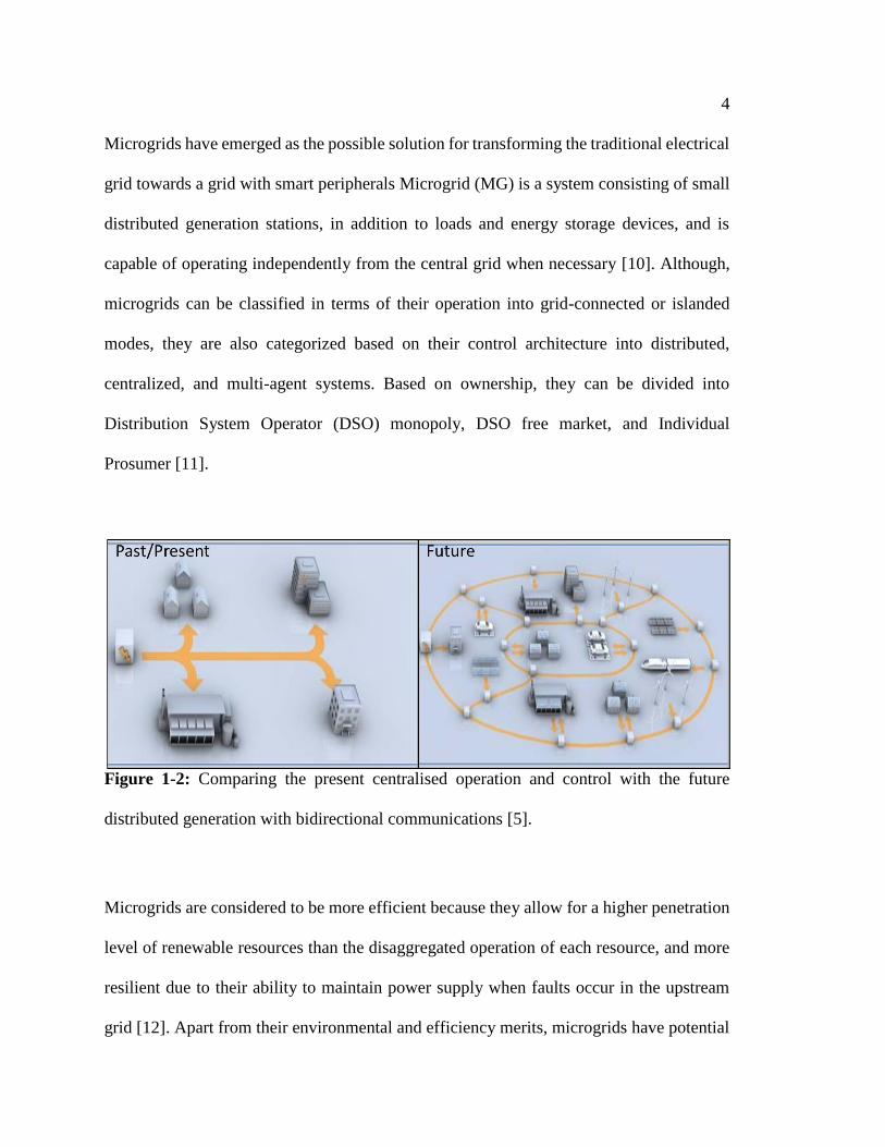
network if generation surpasses the local consumption [9]. Figure 1-2 juxtaposes the

characteristic layout and information flow in a conventional grid system and an integrated

distributed generation network. One can easily observe the need for intelligent multi-

directional communication among the distributed energy resources.

4

Microgrids have emerged as the possible solution for transforming the traditional electrical

grid towards a grid with smart peripherals Microgrid (MG) is a system consisting of small

distributed generation stations, in addition to loads and energy storage devices, and is

capable of operating independently from the central grid when necessary [10]. Although,

microgrids can be classified in terms of their operation into grid-connected or islanded

modes, they are also categorized based on their control architecture into distributed,

centralized, and multi-agent systems. Based on ownership, they can be divided into

Distribution System Operator (DSO) monopoly, DSO free market, and Individual

Prosumer [11].

Figure 1-2: Comparing the present centralised operation and control with the future

distributed generation with bidirectional communications [5].

Microgrids are considered to be more efficient because they allow for a higher penetration

level of renewable resources than the disaggregated operation of each resource, and more

resilient due to their ability to maintain power supply when faults occur in the upstream

grid [12]. Apart from their environmental and efficiency merits, microgrids have potential

5

to strengthen national security by providing a stable, diverse, domestic energy supply [13].

According to the US Department of Defence, more than forty military bases either have

operating microgrids or are developing microgrid technologies [14]. This underscores the

suitability of microgrids for deployment in not only remote locations, but also in critical

and high security areas. They have also been recommended for improving the capabilities

of an off-grid mobile disaster medical response in the healthcare sector, by supporting

prolonged interventions in potentially austere environments while minimizing

environmental footprint [15]. Additionally, on-site production of energy reduces the

amount of power that must be transmitted from centralized plant, and avoids the resulting

transmission and distribution losses as well as the associated costs [12].

However, the implementation of microgrids faces many obstacles. Controlling multiple

generation sources and loads to meet the demand requirements and to maintain the

microgrid’s stability without exceeding any of the operating limits is a complex task [12].

The distributed energy resources of the microgrid have to be coordinated to efficiently and

reliably meet operational requirements (e.g. satisfying power demand in an uninterrupted

manner) in the face of uncertainties arising from renewables, consumers, and the market.

Therefore, efficient energy management is the key to realizing many of the benefits

associated with microgrids. Substantial research efforts have been devoted to developing

methods and techniques for intelligent operation of microgrids within the larger electricity

grid.

1.2 Problem Statement and Thesis Contributions

The focus of this work is on the optimal energy management of a set of microgrid

technologies consisting of a wind turbine (WT), solar photovoltaic (PV) system, battery

6

energy storage system (BESS), a microturbine (MT) and utility grid connection. The goal

is to develop an operational scheduling strategy that allows all the microgrid components

to be operated seamlessly and in sync – in the face of uncertainties from wind power, solar

power, electricity price, and load demand – in order to ensure high penetration of renewable

energy and regular satisfaction of the local load demand at the minimum net cost. To

achieve this purpose requires the application of suitable modelling and optimization

techniques to develop an energy management method which offers less tedious

computational effort, in addition to being able to handle the fast dynamic uncertainties that

are characteristic of renewable energy resources. Figure 1-3 shows the hybrid energy

system setup in consideration. Component selection and sizing is adopted from an existing

microgrid Smart House in Lambton College, Ontario.

Figure 1-3: Microgrid system components and their specifications based on the existing

system in Lambton College, Ontario. System information includes; real-time electricity

7

pricing, weather data and battery state of charge. The EMS integrates the units through a

collective economical operation problem formulation.

The essence of this study is to develop the energy management system through the

following contributions:

Adaptations of system-level models of the microgrid’s components from

established literature sources.

Parameterizations of renewable resource variations using an adaptive mesh

scheme.

Application of a parametric optimization algorithm (MPP) for the optimal

operational scheduling of the entire configuration.

The chosen modelling approach leads to a significant reduction in problem dimensionality,

and hence, computational burden. The uncertain coordinates of wind and solar resources

are parameterized in Cartesian space resulting in improved uncertainty handling.

Consequently, the energy management problem, which is essentially an optimization

problem under uncertainty, is transformed into a multi-parametric optimization problem.

The nature of the problem formulation and the attributes of the solution routine assures

efficiency and optimality of recommended operational decisions. Figure 1-4 shows the

interactions between an energy management routine and a microgrid system. Unlike most

conventional algorithms which require multiple calls on the optimizer during microgrid

system operation, MPP modifies the optimizer into an offline optimal solution reference

map for online decision making.

8

Figure 1-4: Energy management in a microgrid via bidirectional communication between

the energy system components and the optimizer.

Going forward, in chapter two, I discuss the literature efforts to tackle similar energy

management problems. In chapter three, the methodology of the parametric optimization

approach is illustrated. Under chapter four, I present the results of the simulations and go

further to talk about their implications. And lastly, chapter five contains the conclusions

drawn from this work and recommendations for future research efforts.

9

Literature Review

Energy management algorithms can be categorized using the structural and compositional

attributes of the governing mathematical model. Three broad categories can be identified:

those with separate optimization and control routines (e.g. scheduling algorithms) [16-23];

those with coupled optimization and control routines (e.g. MPC-based algorithms) [5, 24-

29]; and those which combine control routines with specified operating rules (e.g. fuzzy

expert algorithms) [30-35]. Section 2.1 of this chapter briefly introduces the role of

optimization and control in energy management. Then in section 2.2, up-to-date theory and

techniques of energy management are reviewed. Lastly, section 2.3 presents various

system-level models of the hybrid energy systems considered in this work.

2.1 Fundamentals of Optimization and Control

For practical implementation, energy management systems usually have an optimization

layer and a control system. Specifically, the optimizer generates the optimal operational

decisions and the job of the control system is to keep the microgrid on that desired

operational trajectory. Below, some basic concepts of optimization and control are

discussed.

2.1.1 Optimization

Optimization is concerned with selecting the best among a set of many solutions by

efficient quantitative methods. It has evolved from a methodology of academic interest into

a technology that has and continues to make significant impact in industry [36].

Optimization can take place at many levels in a system; ranging from individual equipment

to subsystems in a piece of equipment. Optimization problems can be primarily classified

10

in terms of continuous and discrete variables. They can also be classified as; single or

multiple variable, linear or nonlinear, convex or nonconvex, differentiable or non-

differentiable, steady state or dynamic, heuristic or robust, deterministic or optimization

under uncertainty [36-38]. A typical programming (optimization) problem can be

expressed as

𝑀𝑖𝑛𝑖𝑚𝑖𝑧𝑒 𝑓(𝑥) → 𝑶𝒃𝒋𝒆𝒄𝒕𝒊𝒗𝒆 𝒇𝒖𝒏𝒄𝒕𝒊𝒐𝒏

𝑺𝒖𝒃𝒋𝒆𝒄𝒕 𝒕𝒐: 𝒉(𝒙) = 𝟎 → 𝑬𝒒𝒖𝒂𝒍𝒊𝒕𝒚 𝒄𝒐𝒏𝒔𝒕𝒓𝒂𝒊𝒏𝒕𝒔

𝑔(𝑥) ≤ 0 → 𝑰𝒏𝒆𝒒𝒖𝒂𝒍𝒊𝒕𝒚 𝒄𝒐𝒏𝒔𝒕𝒓𝒂𝒊𝒏𝒕𝒔

𝐷𝑖𝑚𝑒𝑛𝑠𝑖𝑜𝑛{ℎ} = 𝑚

𝐷𝑖𝑚𝑒𝑛𝑠𝑖𝑜𝑛{𝑥} = 𝑛

(1)

If 𝑛 > 𝑚, then degrees of freedom is greater than zero and they must be selected in order

to optimize the objective function.

The following optimization terminologies deserve mentioning:

Feasible Solution: set of variables that satisfy equality and inequality constraints.

Feasible Region: the region of feasible solutions.

Optimal Solution: a feasible solution that provides the optimal value of the

objective function.

Convex Function: a function 𝑓(𝑥) is convex if and only if for any two different

values of 𝑥; 𝑥1, 𝑥2, lying in the region R:

𝑓(𝛼𝑥1 + (1 − 𝛼)𝑥2) ≤ 𝛼𝑓(𝑥1) + (1 − 𝛼)𝑓(𝑥2) ∀𝛼 ∈ (0,1) (2)

11

Convex Region: a region is convex if and only if for any 𝑥1, 𝑥2 in the region,

there is an X which can be defined as:

X = α𝑥1 + (1 − 𝛼)𝑥2 ∀𝛼 ∈ (0,1) (3)

By implication, X must always lie in the region. Figure 2-1 is a graphical

illustration of the convex and non-convex regions concept.

Figure 2-1: Convex (left) and non-convex (right) regions.

The nature of the solution search region has an important bearing on the potential for

obtaining suitable results in optimization. In other words, it can be a guide on determining

whether a solution is a local or the global optimum. Figure 2-2 depicts the influence of the

nature of a feasible region on optimality of solutions. The generalized optimization

problem shown in equation (1) can be categorized using the form of the equations and the

type of the variables into:

I. Linear Programming (LP)

𝑓(𝑥), 𝐿𝑖𝑛𝑒𝑎𝑟 𝑓𝑢𝑛𝑐𝑡𝑖𝑜𝑛

𝒉(𝒙), 𝒈(𝒙), 𝑳𝒊𝒏𝒆𝒂𝒓 𝒇𝒖𝒏𝒄𝒕𝒊𝒐𝒏𝒔 (4)

12

II. Non-linear Programming (NLP)

(𝐚) 𝑈𝑛𝑐𝑜𝑛𝑠𝑡𝑟𝑎𝑖𝑛𝑒𝑑min 𝑓(𝑥)

𝒇(𝒙):𝑵𝒐𝒏𝒍𝒊𝒏𝒆𝒂𝒓 (5)

(𝐛) 𝐶𝑜𝑛𝑠𝑡𝑟𝑎𝑖𝑛𝑒𝑑 𝑚𝑜𝑑𝑒𝑙

𝒉(𝒙), 𝒈(𝒙):𝑵𝒐𝒏𝒍𝒊𝒏𝒆𝒂𝒓 (6)

III. Mixed-integer (Linear or Non-linear) Programming

𝐶𝑜𝑛𝑡𝑎𝑖𝑛𝑠 𝑐𝑜𝑛𝑡𝑖𝑛𝑢𝑜𝑢𝑠 (𝑥)𝑎𝑛𝑑 𝑑𝑖𝑠𝑐𝑟𝑒𝑡𝑒 (𝑦) 𝑣𝑎𝑟𝑖𝑎𝑏𝑙𝑒𝑠

𝑦 ∈ 𝑌

𝑥 ∈ 𝑋

(7)

Figure 2-2: Optimal solutions of a constrained non-convex maximization problem

indicating how the nature of the feasible region could affect solution quality.

13

A number of techniques exist for solving these problems and can be generally classified

into direct and indirect (derivative-based) search methods. Some examples can be listed as

follows:

Indirect Search Methods: use derivatives in determining search direction

- Newton method

- Quasi-Newton

- Steepest descent

- Conjugate gradient

Direct Search Methods: rely on function evaluation to choose search direction

- Simplex method

- Random methods (e.g. random walk/jump, simulated annealing)

- Nelder and Mead simplex

- Biologically inspired algorithms (e.g. GA, EP, ACO, PSO, SFLA)

2.1.2 Control

The role of control is to ensure that a system stays on the desired operational trajectory. To

do this, the control mechanism has to depend on the mathematical model of the system.

Figure 2-3 shows a typical block diagram of an optimal control loop. Models for control

are mostly written in state-space form as

��(𝑡) = 𝐴𝑥(𝑡) + 𝐵𝑢(𝑡), 𝐴 ∈ 𝑅𝑛×𝑛, 𝐵 ∈ 𝑅𝑚×𝑚

𝑦(𝑡) = 𝐶𝑥(𝑡) + 𝐷𝑢(𝑡), 𝐶 ∈ 𝑅𝑠×𝑛, 𝐷 ∈ 𝑅𝑠×𝑚

𝑥 ∈ 𝑅𝑛: 𝑠𝑦𝑠𝑡𝑒𝑚 𝑠𝑡𝑎𝑡𝑒

𝑢 ∈ 𝑅𝑚: 𝑠𝑦𝑠𝑡𝑒𝑚 𝑖𝑛𝑝𝑢𝑡 (𝑚𝑎𝑛𝑖𝑝𝑢𝑙𝑎𝑡𝑒𝑑 𝑣𝑎𝑟𝑖𝑎𝑏𝑙𝑒)

(8)

14

𝑦 ∈ 𝑅𝑠: 𝑠𝑦𝑠𝑡𝑒𝑚 𝑜𝑢𝑡𝑝𝑢𝑡 (𝑐𝑜𝑛𝑡𝑟𝑜𝑙𝑙𝑒𝑑 𝑣𝑎𝑟𝑖𝑎𝑏𝑙𝑒)

The control system (controller) is the process of manipulating certain system variables

(inputs) to obtain a desired system output. In predictive control, the discrete-time

counterpart of equation (8) is often used, which is expressed as

𝑥(𝑡 + 1) = 𝐴𝑥(𝑡) + 𝐵𝑢(𝑡)

𝑦(𝑡) = 𝐶𝑥(𝑡) + 𝐷𝑢(𝑡) (9)

Figure 2-3: Block diagram of optimization-based predictive control system

implementation.

The idea is to use the pre-existing input level(s), 𝑢(𝑡 − 1), the currently measured system

variable(s), 𝑦(𝑡), and the calculated system variable(s), 𝑥(𝑡), to determine what the input

level must be presently, 𝑢(𝑡), until the next time step.

Control is a crucial enabling technology for the deployment of renewable energy systems

[13]. Since a distributed generation network can have high number of units, a coordination

strategy is required. A functional analysis of microgrids indicate that a hierarchical and

15

distributed control system is favoured. This hierarchical structure is broadly classified into

three levels based on time scales and purpose as: primary, secondary, and tertiary [39-43].

Primary Control: This is the first control level with the fastest response. The time

scale is a few seconds to a few minutes. It relies on locally measured signals to

respond to system dynamics. Examples can be the maximum power point tracking

in a PV system or the pitch angle control in a WT.

Secondary Control: The secondary layer is the energy management system of an

isolated microgrid, and can facilitate microgrid synchronization with the main

grid. The time frame is slower here; from minutes to some hours.

Tertiary Control: This is the multi-agent level of control, which can champion

specified objectives for a network of microgrids within a couple of days to weeks

or months, time frame.

Soroush and Chmielewski [44] suggested that hierarchical control methods tend to yield

improvements in conversion efficiency, grid coordination and reduction in equipment

fatigue for renewable energy systems. Their various time-scales can be exploited to

construct a control system hierarchy [44]. Figure 2-4 is a schematic illustration of the

various time and length scales in power systems engineering. Each control layer might

involve some form of optimal control with similar or varied objectives. Among the other

benefits, hierarchical control can lead to enhanced system security due to the multiple

control points.

Microgrid control involves both exogenous (consumer load, resource availability, price

profile, etc.) and endogenous (related to the internal system state dynamics) factors [28].

16

At each layer, the control set-point or reference state could be optimal, suboptimal or non-

optimal - depending on the operational objectives and how the reference trajectory is

generated. In most situations, the desire could be to either achieve power balance or attain

some economic requirements.

Figure 2-4: Power systems management and control hierarchies.

2.2 Microgrid Energy Management

One of the most critical and practical challenge towards the practical realization of

distributed energy systems (DES) is related to their operation and overall management [12].

Energy management in microgrids can be considered as a large-scale optimization

problem: given information on the current state of the system and (mostly uncertain) future

changes in pricing, consumptions preferences, distributed generation potentials, and

policy; the optimal decisions on how devices and systems should be operated are made.

Majority of energy management literature are concerned with operational scheduling.

17

However, to implement a schedule, control system design is required at the unit level to

enforce the optimal trajectory generated by the optimization layer [13, 45]. Nevertheless,

there are situations where the control set-points could be based on other factors other than

the economically or environmentally optimal. For instance, energy management may be

required to only maintain power balance.

Scheduling approaches under uncertainty can be classified into reactive and proactive

types [46]. A reactive method modifies a nominal plan, obtained by a deterministic or

stochastic procedure, to adjust it to the updated system data (e.g. model predictive control,

receding horizon optimization, rolling horizon scheduling). Proactive scheduling is used to

generate a plan that satisfies all possible scenarios (e.g. robust optimization, stochastic

optimization). Scheduling approaches should not only be able to generate high-quality

schedules but also to react speedily to unexpected changes and to revise schedules in a

cost-effective manner [45].

Microgrid optimal energy management problems often have objective functions that may

include cost or profit (continuous) functions and activation or deactivation (binary)

decisions [6, 8]. The solution methods can be broadly divided into heuristic and

deterministic routines. Heuristic methods allow for a reasonable solution to a difficult

problem to be obtainable, albeit mostly at the expense of any systematic form of guarantee

of optimality [20, 47-50]. Deterministic algorithms assume some level of understanding of

the sources of system uncertainty; which makes the set of expected outcomes to be finite,

thereby providing for closed form solution(s) of the problem to be attainable [51-53].

Admittedly, it is not always a black and white affair as most algorithms tend to combine

both methods in practice [54, 55]. Some of the commonly used optimization algorithms in

18

energy management include: Genetic Algorithms (GA) [21, 56], Particle Swam

Optimization (PSO) [57-60], Lagrangian Relaxation [49], MPC [61, 62], RHO [63, 64]

PEM-FA [9], and PEM-IBA [65].

Greenhouse gas (GHG) emissions reduction has been also incorporated in the optimization

formulations, resulting in multi-objective optimization problems that can be solved to

Pareto optimality using a number of heuristic techniques. [6, 8, 66-68]. Optimal operation

problems have also been solved by embedding a non-model-based scheme, such as fuzzy

logic or artificial neural networks, under an optimal power flow layer [33, 69-71]. This

allows the training of the embedded layer with results from the optimal power flow

problem [8]. Such an arrangement has sparked interests because it does not require detailed

model of the system and is robust to sudden changes in system parameters [8, 39].

Zhong et al. in [20], developed a modified Shuffled Frog Leap Algorithm (SFLA) – a meta-

heuristic method based on the behaviour of a group of frogs when searching for food - to

capture a distributed generation planning problem with the aim of minimizing generation

and emissions cost. In comparing their results with the original SFLA, they noted that their

improvement was able to overcome the limitations of the original SFLA which is prone to

being trapped at a local optimum. Also, they observed that the modified SFLA did better

than GA and Evolutionary Programming (EP) in terms of computational time and

optimality.

Li and coworkers [65] combined an Improved Bat Algorithm (IBA) and point estimation

method to optimize the operation of microgrid. Using point estimation method – based on

probability density functions and static moments of random variables – to deal with the

uncertainty in load demand and output power of solar and wind installations; IBA is used

19

to solve the optimal operation problem. IBA is a modification of the original bat algorithm

(BA) which gets easily trapped at a local minimum. It has the capability to switch between

local and global search modes through an adaptive weighting factor or a chaotic variable.

Final results are expressed in terms of the optimal operating cost distribution, which can

be implemented based on realized system states. Therefore, optimal operation is only

guaranteed for only the scenarios considered in the uncertain variables.

X. Lei and coworkers in [72] presented an optimal energy trading problem between a DSO

and a microgrid agent. They formulated the problem as a bi-level optimization; where the

upper-level objective is to maximize the profit of the DSO while the lower-level aims to

maximize profit for the microgrid agent. Their model generates the optimal energy

schedules and determines the bid/offer price at which the microgrid agent should buy and

sell electricity from/to the grid. They showed that it is possible to achieve both desired

objectives in the DSO free market arrangement.

Moreover, literature is replete with the application of the MPC framework in energy

management problems, due to the ability of the framework to incorporate both economic

and control goals in its formulations while reacting at flexible timescales to system

dynamics. MPC is an optimization-based control approach where an optimization problem

is formulated and solved at each discrete time-step, as an integral part of a control strategy.

Figure 2-5 is a block diagram of an MPC scheme, while Figure 2-6 shows the

implementation procedure of an MPC-based algorithm. It is an appealing method for

microgrid energy management because control actions are implemented in awareness of

possible future states of the system.

20

Figure 2-5: Model predictive control scheme block diagram

At each time-step, the solution to the optimal control problem is obtained over a desired

prediction horizon using an updated system state information. Hence, the control sequence

over a specified horizon is also obtained, but only the control action at the next time-step

is applied, and the entire process is repeated again. Typically, in MPC, the objective

function penalizes deviations of the states and inputs from their reference (optimal) values,

while constraints are enforced explicitly [28]. Results improve with higher optimization

horizons, however, computational expenses also increase and problem can become too big

to solve in reasonable time. Besides, accuracy of model parameters or forecast information

decreases with longer horizons, which will affect the obtained solutions [8].

21

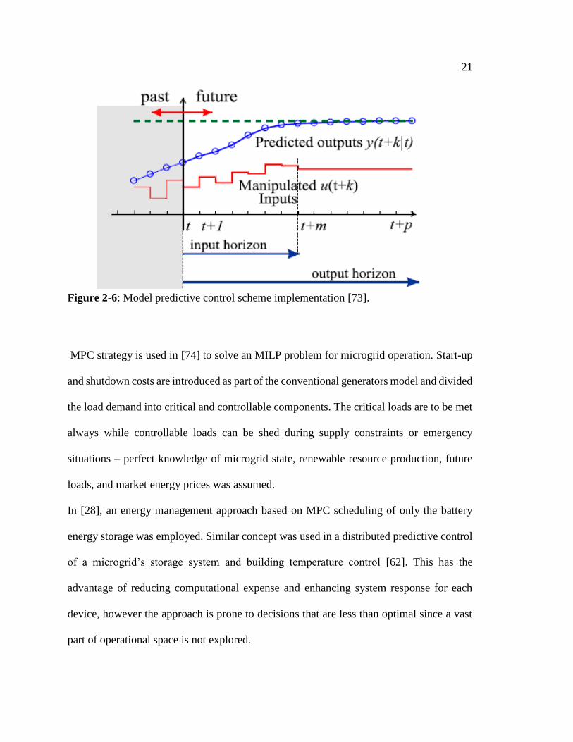
Figure 2-6: Model predictive control scheme implementation [73].

MPC strategy is used in [74] to solve an MILP problem for microgrid operation. Start-up

and shutdown costs are introduced as part of the conventional generators model and divided

the load demand into critical and controllable components. The critical loads are to be met

always while controllable loads can be shed during supply constraints or emergency

situations – perfect knowledge of microgrid state, renewable resource production, future

loads, and market energy prices was assumed.

In [28], an energy management approach based on MPC scheduling of only the battery

energy storage was employed. Similar concept was used in a distributed predictive control

of a microgrid’s storage system and building temperature control [62]. This has the

advantage of reducing computational expense and enhancing system response for each

device, however the approach is prone to decisions that are less than optimal since a vast

part of operational space is not explored.

22

Biyik and Chandra in [75] presented an MPC approach for optimal supervisory control of

microgrids. In their work, they decomposed the optimal operational planning problem into

two layers: a unit commitment (UC) problem at the upper layer and an optimal dispatch

(OD) at the lower layer. They further recast the UC into a pure integer programming

problem, leaving the OD as a linear programming problem – which leads to improved

solution efficiency via memory economy and execution speed. However, this approach is

better suited for worst-case complexity and scalability considerations; and not for when

optimality is of utmost importance.

Marinelli et al. in [34] suggested the use of predictive control strategy based on day-ahead

meteorological forecasts to schedule hourly power production by means of proper

management of the storage system. The approach is limited by unavoidable forecast errors

and inaccuracies in model parameters. They further proposed that storage systems or

controllable loads should be used for buffering forecast errors, by incorporating

meteorological forecast errors into storage system design. Ultimately, prediction accuracy

of wind and solar resource availability is the major issue in predictive algorithms [5].

Point estimate method (a derivative of the approximation method) was used to account for

uncertainties in the electricity market price, load demand, wind and solar power [9]. The

energy management problem was formulated as a nonlinear constraint optimization

problem to minimize total operating cost. By modelling uncertain input variables with the

Weibull and normal distributions, they deployed a modified firefly algorithm to solve the

optimal operational planning problem.

Su and coworkers in [52], developed a stochastic energy management scheme to minimize

operational cost and power losses in a grid-connected microgrid. They decomposed their

23

formulation into a master problem and sub-problem; where the energy scheduling master

problem is solved for various wind and solar power generation scenarios obtained from

Monte Carlo simulations. Solutions of the master problem are then verified with power

flow constraints, which constitutes the subproblem.

A risk-based optimal scheduling and operation of microgrids was developed using

operational volatility measures and associated risks [76]. It was shown that substantially

different results can be obtained when compared to traditional optimization system

behaviour without explicit risks. However, the model assumed that load demand is

considerably higher than what can be produced from renewable sources, so conventional

sources have to be engaged at all times.

Caldognetto et al. in [77] proposed a distributed cooperative control technique for

microgrids with the aim of optimizing the components of the microgrid individually, but

with effective bidirectional information sharing among the units. The authors argued that

centralized control is impractical for wide networks of distributed energy resources. This

approach will not be suitable for a DSO monopoly operated microgrid because optimal

scheduling of each component of the system may not translate overall system operational

optimality.

Deckmyn et al. in [78] developed a quadratic multi-objective environomic formulation that

minimizes both costs and emissions of the internal production and imported energy from

the utility grid, for a grid-tied microgrid. By assuming prescient knowledge of electricity

demand, price and renewable resource availability using real data, they modelled the cost

and emissions variables as polynomial functions of the generators active power output, and

solved the problem using GA.

24

In their work, conventional generators and grid connection supplemented the net

requirement between power demand and the harnessed renewable energy.

𝐶𝑖(𝑃𝐺𝑖) =∑𝑎𝑖

𝑁𝐺

𝑖=1

+ 𝑏𝑖𝑃𝐺𝑖 + 𝑐𝑖𝑃𝐺𝑖2 (10)

𝐸𝑖(𝑃𝐺𝑖) =∑𝑎𝑒

𝑁𝐺

𝑖=1

+ 𝑏𝑒𝑃𝐺𝑖 + 𝑐𝑒𝑃𝐺𝑖2 (11)

Where 𝑎𝑖, 𝑏𝑖, and 𝑐𝑖 are the fuel cost coefficients for the individual generating units, 𝑃𝐺𝑖

the active power output of the 𝑖th generator, 𝐶𝑖 the fuel cost function, 𝐸𝑖 the emission

function and 𝑁𝐺 is the number of generators [78].

In [79], a sliding-window based algorithm was proposed for real-time microgrid energy

management by assuming that the renewable energy off-set by the load over time (net

energy profile), was predictable with high accuracy. The net energy profile was known

ahead of time, then an off-line optimization problem was solved to minimize the total

energy cost of conventional generation. The obtained closed form solution from the off-

line optimization was then applied into their online optimisation algorithm, by introducing

noise to the earlier predicted net energy profile. The proposed online algorithm uses the

idea of receding horizon optimization (RHO), where the discrepancy between the off-line

and online solutions are known up to the current time but future errors are unknown to the

system. The effectiveness of the algorithm depends on the accuracy of modelling the net

energy profile in the off-line solution; which can result in additional computational task

over the purely online techniques.

25

X. Wang et al. in [80] applied RHO in the energy management of a microgrid that supports

a chlor-alkali process. The idea of Enterprise-wide Energy Optimization (EWEO) was used

to consider the optimal dispatch of electricity generation among all available resources as

well as the operation of manufacturing facilities that often require extensive energy use.

They embedded an open source weather forecasting tool known as Weather Analytics, to

obtain hourly resolutions of weather prediction. With the objective of minimizing operating

and environmental costs, RHO –the first layer in MPC – generates optimal set points for

the energy system components and returns results for control system action. Economic

receding horizon optimization was able to manage uncertainties and reduce computational

complexity [80]. This is because RHO decouples control and optimization, unlike MPC,

and thereby might involve lesser dimensionality.

Silvente et al. [46] applied a rolling horizon scheme (RH) – a form of RHO – which uses

periodic input data updates to generate scheduling strategies for optimal coordination of

energy production and consumption in microgrids. They developed the concept of

consumption tasks to divide the total demand within the operational horizon into flexible

demand profiles. They applied penalty costs for delays in the nominal energy demands.

The problem formulation takes into account not only the production and storage levels to

be managed by the microgrid , but also the possibility to modify the timing of the energy

consumption. For a given energy demand, given by the amount of energy required by a set

of energy consuming tasks (𝑗, 𝑓), where 𝑓 ∈ 𝐹𝑗 denotes the 𝑓𝑡ℎ time that the consumer 𝑗 is

active. The following big-M logical restrictions apply:

(𝑡 − 𝑇𝑠𝑗,𝑓) − (1 − 𝑌𝑗,𝑓,𝑡) × 𝑀 ≤ 0 ∀𝑗, 𝑓 ∈ 𝐹𝑗𝑅𝐻 (12)

26

(𝑡 − 𝑇𝑠𝑗,𝑓) + (1 − 𝑌𝑗,𝑓,𝑡) × 𝑀 ≥ 0 ∀𝑗, 𝑓 ∈ 𝐹𝑗𝑅𝐻 (13)

(𝑡 + 1 − 𝑇𝑓𝑗,𝑓) − (1 − 𝑍𝑗,𝑓,𝑡) × 𝑀 ≤ 0 ∀𝑗, 𝑓 ∈ 𝐹𝑗𝑅𝐻 (14)

(𝑡 + 1 − 𝑇𝑓𝑗,𝑓) − (1 − 𝑍𝑗,𝑓,𝑡) × 𝑀 ≥ 0 ∀𝑗, 𝑓 ∈ 𝐹𝑗𝑅𝐻 (15)

Where 𝑇𝑠𝑗,𝑓 is the start consumption time and 𝑇𝑓𝑗,𝑓 the final consumption time; at the

beginning and end of each consumption task (𝑗, 𝑓). Binary variable 𝑌𝑗,𝑓,𝑡 is active when

energy consumption (𝑗, 𝑓) starts at time period 𝑡 of the prediction horizon. Also, binary

variable 𝑍𝑗,𝑓,𝑡 is active when the consumption task (𝑗, 𝑓) finishes at time period (𝑡 + 1).

For each energy consuming task, its duration and a target starting time are established.

Moreover, tasks can be delayed within specified limits, generating a penalty cost. And all

tasks which might be active during each iteration of the rolling horizon approach are

included in the dynamic set 𝐹𝑗𝑅𝐻. They concluded that longer prediction horizons favour

the generation of better solutions, at the expense of further computational time.

Trifkovic et al. in [81] applied dynamic real-time optimization (DRTO) and control to

energy management in a hybrid energy system. The energy management structure

consisted of two layers – upper and lower. At the upper layer an optimal dispatch problem

was solved to generate set-points for local controllers which constitute the lower layer. The

local controllers were required to enforce the optimal trajectories. The approach requires

accurate weather forecast (which is not easily achieved - [80]) and demand prediction in

order to maintain the system on the optimal trajectory. Otherwise, sub/non-optimal

contingency decisions have to be made each time simulation conditions differ from actual

27

meteorological conditions, due to faster system dynamics with respect to problem solution

time.

The same authors implemented a two level control system for power management of a

standalone renewable energy system [82]. A supervisory layer at the top is used to ensure

power balance between generation sources, storage, and dynamic load demand. Local

controllers at the bottom guide individual system components towards achieving the

collective control target reached at the supervisory level. Detailed model of each system

component was developed to serve as a platform for implementation of more advanced

supervisory control strategies.

Ulbig et al. in [83] proposed a framework for multiple time-scale cascaded MPC for power

system control and optimization. They emphasized that using a single MPC scheme for

power systems control on several time-scales can be computationally prohibitive. Using

two separate MPC schemes; a higher-level MPC takes charge of power dispatch and passes

decisions to the lower-level MPC which takes care of frequency regulation. Interactions

between the two control layers is accomplished via updates of constraint and cost terms in

the respective MPC setups. The frequency regulating MPC setup checks whether or not

positive and negative regulation reserves will be sufficient for every hourly time-step of

the power dispatch process. Besides, actual implementation of control decisions at each

system component is realised in the form of an explicit MPC scheme that is pre-computed

off-line. The issue with this approach is that part of the common operational space to the

entire power system can be lost as a result of the subdivisions of the control structure,

which can lead to a false sense of optimality of computed operational trajectory.

28

Fossati et al. in [84], solved an optimal operation problem in microgrids by interfacing two

genetic algorithms through a hybridization of fuzzy systems and genetic algorithms. One

subroutine solves the optimal day-ahead microgrid scheduling problem and generates rules

for a fuzzy expert system to control the power output of the storage system, while the

second subroutine is used to tune the membership functions so that the expert system can

be optimized according to the changing load demand, wind power availability and

electricity prices. Fuzzy controllers have been used in [85] for power management of

microgrids in islanded operation through voltage and frequency regulation, to minimize

stress for conventional generators and to maximize the microgrid availability. However,

these approaches require the input data – which includes: battery state of charge, electricity

price, wind power generation and load demand - to be predicted accurately.

Pan and Das [86] applied fractional order (FO) controllers for a microgrid system

operational management via suppression of system frequency deviation in a nonlinear and

stochastic model of a microgrid. Aiming to satisfy power demand (with production from

autonomous microgrid generation elements) and reserve surpluses in a backup storage,

they deployed FO control strategy and used a global optimization algorithm to tune

parameters for the FO-proportional integral derivative (FOPID) controller in order to meet

system performance specifications. They used a Kriging based surrogate modelling

technique to alleviate the issue of expensive objective function evaluation for the

optimization based controller tuning. They observed that the FOPID controller outperforms

the standard PID controller under nominal operating condition and gives better robustness

for large parametric uncertainty of the microgrid. Also, the Kriging based surrogate

29

modelling and optimization reduces the time taken for optimizing the controller parameters

for the microgrid system; which can facilitate online implementation.

A robust optimization (RO) approach for energy management in microgrids was developed

by Kuznetsova et al. in [87]. Uncertainties in renewable power generation and consumption

were modelled using prediction intervals that are estimated by a Non-dominated Sorting

Genetic Algorithm - trained Neural Network (NSGA-NN). They used an agent-based

modelling (ABM) scheme where each microgrid element or stakeholder (i.e. Photovoltaic

power production system, wind power plant, and residential district load) is considered as

an individual agent with a specific goal of either decreasing its expenses from power

purchasing or increasing its revenues from power selling. They argued that the proposed

approach allows identifying the level of uncertainty in the operational and environmental

conditions upon which RO performs better than an optimization based on expected values

– since RO is both data and computationally intensive, and may not be practicable to

capture the entire uncertain variable space.

Hu et al. developed an energy management model based on the effect of power demand

and battery investment on the optimal operational strategies of a microgrid system [88].

They formulated the model as a mixed linear programming problem and used sensitivity

analysis to show the effects of demand growth and battery capacity on optimal operating

decisions. Their work concluded that low energy demand scenarios could result in low

battery efficiencies. Hence, appropriate battery capacity should be determined by the

efficiency of electricity storage devices and electricity production scenarios.

Hittinger et al. in [89] evaluated the value of batteries in microgrid electricity management

systems using an improved energy systems model (ESM). Their model added several

30

important aspects of battery modelling, including temperature effects, rate-based variable

efficiency, and operational modelling of capacity fade. The model is then used to compare

Aqueous Hybrid Ion (AHI) battery chemistry to lead acid (PbA) batteries in standalone

microgrid operation. They observed that the cost-effectiveness of the battery storage

systems depends on the microgrid operational strategy. They noted that operational

scenarios that require constant cycling of batteries favour AHI deployment while

applications that require batteries to serve as a backup energy service rather than a cycling

service will find that PbA batteries are a better choice. They concluded that microgrids

using AHI batteries should be designed and operated differently than similar PbA

microgrids.

In [90], an energy management focus that is based on customer preference satisfaction is

developed as a stochastic optimization model. In contrast to the current and prevalent

lowest cost approach to producing and consuming energy, it used carbon reduction;

pollution reduction; improved reliability; improved quality; renewable usage; and local

generation as stakeholder objectives. It argued that in some sectors, like the military,

security could be given a higher priority than economics.

Alam et al. in [91]., proposed a user-centric cost optimization of distributed generation

systems, where energy users collaborate with their neighbours to participate in energy

trading. Thereby, those participating in the energy pool can avoid buying electricity from

the utility at higher prices by depending on their neighbours’ reserves. They also presented

a method for disaggregating the unified optimization model for the energy pooling

microgrids.

31

Pinceti et al. in [85] described the control functions that a power management system

(PMS) needs to have for controlling a microgrid, with both conventional and renewable

sources. Among them are: a control logic that is suited for grid-connected operation and

islanded mode; fast load or generator shedding actions to preserve system stability during

switches between operation modes. The PMS itself should guarantee the stable operation

of a microgrid in presence of unpredictable variations caused by renewable sources and

loads, and optimize the energy production of renewable and conventional sources.

However, to stabilize a microgrid, especially during isolated operation, requires a

coordinated real-time control of the power generated by conventional generators and by

renewable sources, with control goals that may push towards divergent solutions [85]. For

instance, to reduce energy cost requires maximizing the production of renewable sources,

but safety could require a higher production by conventional sources. Therefore, a power

management must find trade-offs between all these targets based on a rank of priorities

defined by the stakeholders.

Nejad and Tafreshi [58] proposed a model for optimum operation of microgrids using the

concept of controllable and uncontrollable loads. They presented a controlling algorithm

that uses the welfare priorities of consumers to change or postpone the consumption of

controllable loads, with regard to uncertainties in the renewable energy generation and the

energy price of upstream distribution network. They used Monte Carlo simulation to model

the uncertainties in: renewable generation; energy spot price; power consumption of

uncontrollable loads; failure probability of units; and disconnection probability from the

main grid. PSO was used to solve the optimal operation problem, and results were

presented as a probability distribution function for each of the decision variables. They

32

concluded that by implementing controlling methods for loads which could cover

generation variations of non-dispatchable resources or energy price of upstream

distribution network, optimal operation could be achieved. However, the proposed

operation method for microgrids requires a lot of computational effort to be able to handle

the numerous scenarios which it considers.

Li et al. [92] proposed a hierarchical energy management strategy based on the idea of

multiple time-scale coordination with three layers: day-ahead layer, adjustment layer, and

real-time layer. The day-ahead layer uses multi-step optimization techniques and predicted

availability of renewable energy sources to suggest potential operational schedule. The

adjustment layer modifies power set-points of online units by using the available

information at dispatch time; thereby, errors due to forecasted information at the previous

layer is absorbed. Then, the real-time layer maintains the power exchange between the

microgrid and the main grid at the pre-determined value while using the storage system to

balance the fluctuations of net-load. They also prohibited frequent switching of charge-

discharge state to prolong the lifespan of storage devices.

Collazos et al. [93] applied an optimal control technique for energy management in a poly-

generation system with micro-cogeneration capability. The predictive optimal controller

uses mixed-integer and linear programming where energy conversion and energy services

models are defined as a set of linear constraints, and integer variables model the start-up

and shut-down operations as well as the load dependent efficiency of the cogeneration unit.

The MILP aims to minimize overall operating cost combined with a penalty term that is

proportional to the time during which noncompliance to comfort requirements occurs. The

idea of a cyclic horizon – as against open horizon – is also introduced by supposing that

33

the state of the energy system should be recovered after 24 hours of operation if one day

resembles the next. However, the model provided a 1 hour window for the system to

recover whenever the cyclic assumption fails. It was reported that the cyclic horizon

strategy gives a better performance than the common open horizon approach.

Li and Barton [38] presented a stochastic programming formulation for integrated design

and operation of energy systems under significant uncertainties. By casting the problem in

two stages, they transformed it into a large-scale nonconvex mixed-integer nonlinear

programming problem (MINLP). They exploited the decomposable structure of the

problem using an enhanced nonconvex generalized Bender’s decomposition (NGBD) for

efficient global optimization. Their work aimed to ensure that the designed systems can

work under different operating conditions and that it achieves the best total profit over all

the operating modes. They observed improved solution times via piecewise convex

relaxations in the NGBD algorithm. However, the set of uncertain factors must not be

infinite.

From the preceding literature reviews, it is obvious that a lot of research efforts have been

put into the microgrid energy management problem. Overall, various formulations of the

problem and solution strategies have been proffered to cater for the economic, safety,

security, feasibility, reliability, and environmental requirements of an effective energy

management system. However, each of the available algorithms face challenges that border

on, at least, one of the following areas: uncertainty handling, model dimensionality, and

computational complexity.

34

2.3 Microgrid Component Modelling

The essence of modelling is to capture system behaviour in mathematical form. Modelling

can save time and cost of performing experiments or building the pilot of a desired system.

In energy management, the description of the characteristics of technologies are required

to be in the form that enhances the solvability and computational efficiency of the

scheduling problem [12]. Models of the microgrid components are presented below, with

a focus on system level modelling.

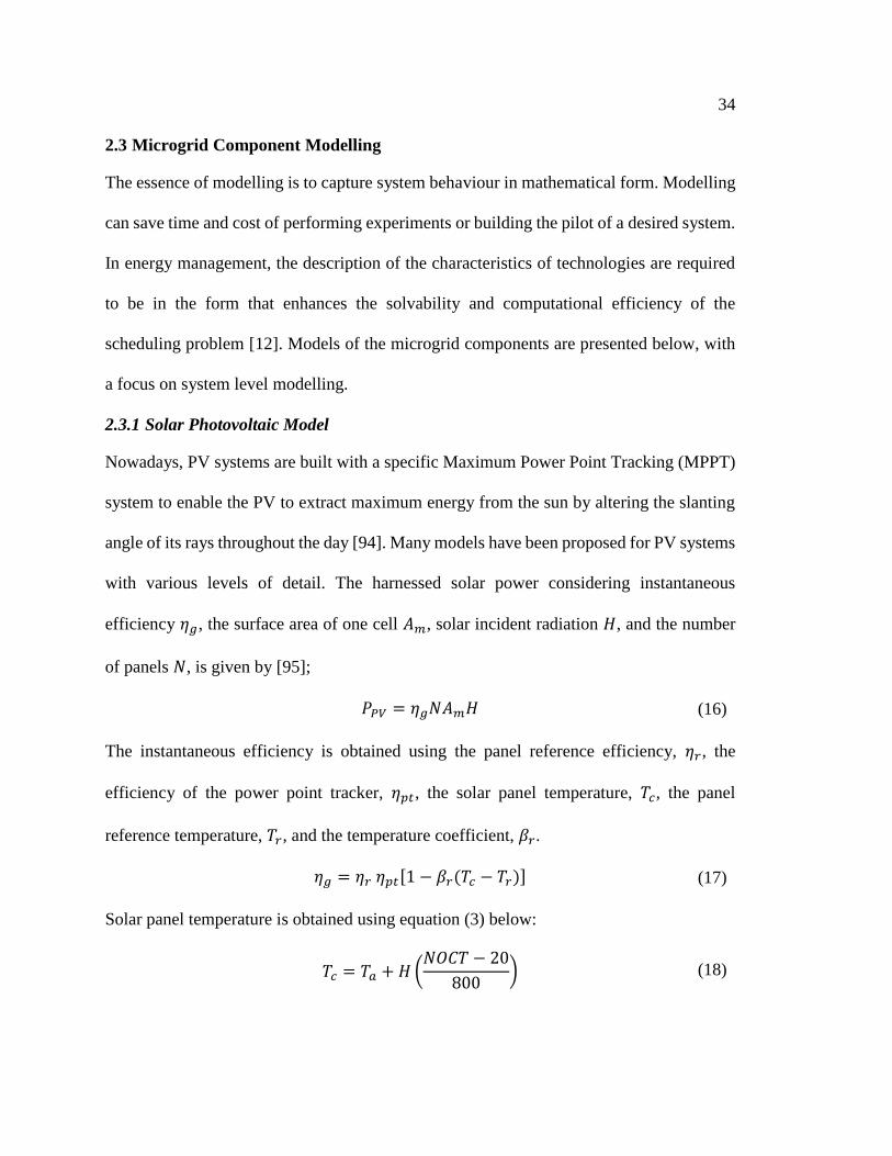
2.3.1 Solar Photovoltaic Model

Nowadays, PV systems are built with a specific Maximum Power Point Tracking (MPPT)

system to enable the PV to extract maximum energy from the sun by altering the slanting

angle of its rays throughout the day [94]. Many models have been proposed for PV systems

with various levels of detail. The harnessed solar power considering instantaneous

efficiency 𝜂𝑔, the surface area of one cell 𝐴𝑚, solar incident radiation 𝐻, and the number

of panels 𝑁, is given by [95];

𝑃𝑃𝑉 = 𝜂𝑔𝑁𝐴𝑚𝐻 (16)

The instantaneous efficiency is obtained using the panel reference efficiency, 𝜂𝑟, the

efficiency of the power point tracker, 𝜂𝑝𝑡, the solar panel temperature, 𝑇𝑐, the panel

reference temperature, 𝑇𝑟, and the temperature coefficient, 𝛽𝑟.

𝜂𝑔 = 𝜂𝑟 𝜂𝑝𝑡[1 − 𝛽𝑟(𝑇𝑐 − 𝑇𝑟)] (17)

Solar panel temperature is obtained using equation (3) below:

𝑇𝑐 = 𝑇𝑎 + 𝐻 (

𝑁𝑂𝐶𝑇 − 20

800) (18)

35

Where 𝑇𝑎 is the ambient temperature and 𝑁𝑂𝐶𝑇 is the normal operating temperature which

can be found in the datasheet of any solar cell.

A five parameter solar PV model has also been deployed by some workers as in [80].

However, with an MPPT system, power production of the PV array is shown to be directly

proportional to the incident solar radiation [96]

𝑃𝑃𝑉(𝑡) = 𝑃𝑃𝑉,𝑟𝑎𝑡𝑒𝑑

𝐻(𝑡)

𝐻𝑟𝑎𝑡𝑒𝑑 (19)

Commonly, the rated power refers to the power output at 1000𝑊 𝑚2⁄ and 25℃ [96] -

which is roughly the upper limit of insolation at standard environmental conditions.

2.3.2 Wind Turbine Model

Wind is the most promising source of alternate energy, and has become more affordable

over the past decade [94]. China and USA are the fastest growing wind power countries,

while Germany and Spain have the highest installed generation capacity of the world [1,

94]. The output power of the wind turbine can be calculated from equation (4) below:

𝑃𝑤𝑖𝑛𝑑(𝑡) =

1

2𝜌𝐴[𝑣(𝑡)]3𝐶𝑝 (20)

Where 𝜌 is air density; 𝐴 is the cross-sectional area through which the blade passes; 𝑣 is

the wind speed normal to 𝐴; 𝐶𝑝 is the power coefficient which is related to the ratio of

downstream to upstream wind speeds. Since power in the wind is proportional to the cube

of the wind speed, modest increases in wind speed can have significant economic impact.

The output power of a wind turbine can be related to wind speed using the rated output

power of the design as follows [94]:

36

𝑃𝑤𝑖𝑛𝑑(𝑣) =

{

0 (𝑣 ≤ 𝑣𝑐𝑖 or 𝑣 ≥ 𝑣𝑐𝑜)

𝑃𝑤𝑖𝑛𝑑−𝑟𝑎𝑡𝑒𝑑(𝑣 − 𝑣𝑐𝑖)

(𝑣𝑟 − 𝑣𝑐𝑖) (𝑣𝑐𝑖 ≤ 𝑣 ≤ 𝑣𝑟)

𝑃𝑤𝑖𝑛𝑑−𝑟𝑎𝑡𝑒𝑑 (𝑣𝑟 ≤ 𝑣 ≤ 𝑣𝑐𝑜)

(21)

Where 𝑣𝑐𝑖, 𝑣𝑐𝑜, and 𝑣𝑟 are cut-in, cut-out, and rated wind speeds respectively. 𝑃𝑤𝑖𝑛𝑑−𝑟𝑎𝑡𝑒𝑑

is the rated output power of the WT. The final output power could be reduced by losses. In

[96], the wind power expression is written in terms the fractional availability of the rated

power as

𝑃𝑤𝑖𝑛𝑑(𝑡) = 𝑓𝑤(𝑡) 𝑃𝑤𝑖𝑛𝑑−𝑟𝑎𝑡𝑒𝑑 (22)

𝑓𝑤(𝑡) =

{

0 (𝑣(𝑡) ≤ 𝑣𝑐𝑖 or 𝑣(𝑡) ≥ 𝑣𝑐𝑜)

𝑣(𝑡)3 − 𝑣𝑐𝑖 3

𝑣𝑟3 − 𝑣𝑐𝑖3 (𝑣𝑐𝑖 ≤ 𝑣(𝑡) ≤ 𝑣𝑟)

1 (𝑣𝑟 ≤ 𝑣(𝑡) ≤ 𝑣𝑐𝑜)

(23)

Taller towers can get the turbine into higher winds. The following correction expression is

be used to account for turbine heights:

(𝑣

𝑣0) = (

𝑞

𝑞0)𝛼

(24)

Where 𝑣0 is the wind speed at height 𝑞0 (the reference height), and 𝛼 is a friction coefficient

which is related to the terrain over which the wind blows.

2.3.3 Battery Energy Storage Model

Reliability issues in microgrids are mostly solvable by the integration of robust energy

storage units [14]. In grid-tied operations, the main role of energy storage is to balance

37

supply and demand, to enable integration of renewables into the grid, to store energy during

reduced load and dispatch when demand peaks. In islanded operation, the energy storage

system could be required to supply critical and non-critical loads [14]. Although there are

many energy storage devices, battery or hydrogen tanks are often used as storage systems

in microgrids [94, 97-99]. For batteries, information on the state of charge (SOC) is

paramount. The SOC during the charging or discharging processes can be estimated using

equations (6).

𝑆𝑂𝐶𝑏𝑎𝑡(𝑡) = 𝑆𝑂𝐶𝑏𝑎𝑡(𝑡 − 1)[1 − 𝜎] + [𝐸+(𝑡) − 𝐸−(𝑡)]𝜂𝑏𝑎𝑡 (25)

Where 𝜂𝑏𝑎𝑡 is the battery efficiency, 𝜎 is the rate factor, 𝐸+(𝑡) is the charging power, and

𝐸−(𝑡) is the discharging power. The SOC must be constrained between minimum and

maximum states to safeguard the battery.

𝑆𝑂𝐶𝑏𝑎𝑡 𝑚𝑖𝑛 ≤ 𝑆𝑂𝐶𝑏𝑎𝑡(𝑡) ≤ 𝑆𝑂𝐶𝑏𝑎𝑡 𝑚𝑎𝑥 (26)

State of charge limits are recommended by various literature sources to be between 0.1 and

0.9; to avoid deep discharge and allow for storage leakages. Also, the rate factor (charging

or discharging rate) at any time needs to remain between some bounds as described by the

following condition [28]:

𝜎𝑚𝑖𝑛 ≤ 𝜎 ≤ 𝜎𝑚𝑎𝑥 (27)

In [74], a discrete time dynamic model is created, which discourages simultaneous

charging and discharging of storage unit. Different charging and discharging efficiencies

are used to account for losses, and a parameter that accounts for stored energy degradation

is also introduced.

38

𝑆𝑂𝐶𝑏𝑎𝑡(𝑘 + 1) = 𝑆𝑂𝐶𝑏𝑎𝑡(𝑘) + 𝜂𝑏𝑎𝑡𝐸𝑏𝑎𝑡(𝑘) − 𝐸𝑠𝑏 (28)

𝜂𝑏𝑎𝑡 = {

𝜂𝑐 (𝑐ℎ𝑎𝑟𝑔𝑖𝑛𝑔 𝑚𝑜𝑑𝑒)

1 𝜂𝑑⁄ (𝑑𝑖𝑠𝑐ℎ𝑎𝑟𝑔𝑖𝑛𝑔 𝑚𝑜𝑑𝑒) (29)

Where 𝐸𝑏𝑎𝑡(𝑘) is the power exchanged with storage device at time, 𝑘, 𝐸𝑠𝑏 the natural

stored energy degradation. Generally, the required battery capacity is based on the expected

deficient load, given in [100] as

𝐶𝑏𝑎𝑡 =

𝑁𝑎(𝐸𝐿 − 𝐸𝐺)

𝜂𝑏𝑎𝑡𝜎𝑇𝑓 (30)

Where 𝑁𝑎 is the number of days of autonomy, 𝐸𝐿 the total load demand, 𝐸𝐺 the total

renewable generation, and 𝑇𝑓 the temperature factor.

2.3.4 Microturbine Model

In order to promote green energy, microturbines are mostly used as backup resources

should the battery system be unable to supply the load during operation. Due to decreasing

efficiency at low set points, microturbines have to be constrained to operate above 50% of

their power rating, 𝑃𝑚,𝑟𝑎𝑡𝑒𝑑, [96].

0.5𝑃𝑚,𝑟𝑎𝑡𝑒𝑑(𝑡) ≤ 𝑃𝑚(𝑡) ≤ 𝑃𝑚,𝑟𝑎𝑡𝑒𝑑(𝑡) (31)

From [96], fuel consumption is related to power output as

𝐺𝑚(𝑡) =

𝑃𝑚(𝑡)

𝜂𝑚 (32)

Where 𝐺𝑚 is the gas consumption and 𝜂𝑚 is the electrical efficiency. Commercial

microturbines are available in a limited number of fixed capacities.

39

2.3.5 Electricity Pricing and Load Demand Model

From consumer psychology, different commodity prices will receive different consumer

responses. Consumers tend to decide the best time to buy based on commodity price

changes [101]. Xiaohong et al. in [101] developed an optimal time of use (TOU) price

based on economic operation of microgrids and the demand side response. Using power

supply enterprise benefit maximization as the objective, they showed that the best time of

use price and optimal scheduling scheme can be made according to the load demand

prediction.

A lot of researchers have suggested that the rate of change in load demand (load shifting)

and electricity price differences can be approximately expressed by piecewise linear

functions [101-107]. By classifying loads into valley, flat, and peak; the load – price

dynamics is categorized into three, along with their corresponding load shifting curves

[101], as follows:

Load changing rate from peak to valley

𝜆𝑝𝑣 = {

0 (0 ≤ ∆𝑝𝑝𝑣 < 𝑎𝑝𝑣)

𝐾𝑝𝑣(Δ𝑝𝑝𝑣 − 𝑎𝑝𝑣) (𝑎𝑝𝑣 ≤ ∆𝑝𝑝𝑣 < 𝑏𝑝𝑣)

𝜆𝑝𝑣𝑚𝑎𝑥 (∆𝑝𝑝𝑣 ≥ 𝑏𝑝𝑣)

(33)

Where Δ𝑝𝑝𝑣 is the electricity price difference between peak and valley, 𝑎𝑝𝑣 is the

minimum load shifting from peak to valley, 𝑏𝑝𝑣 is the maximum load shifting

from peak to valley, 𝐾𝑝𝑣 is the slope of linear zone in the load shifting curve (see

figure below), 𝜆𝑝𝑣𝑚𝑎𝑥 is the maximum load shifting rate from peak to valley.

40

Figure 2-7: Load shifting curve from peak to valley [101].

Load changing rate from flat to valley

𝜆𝑓𝑣 = {

0 (0 ≤ ∆𝑝𝑓𝑣 < 𝑎𝑓𝑣)

𝐾𝑓𝑣(Δ𝑝𝑓𝑣 − 𝑎𝑓𝑣) (𝑎𝑓𝑣 ≤ ∆𝑝𝑓𝑣 < 𝑏𝑓𝑣)

𝜆𝑓𝑣𝑚𝑎𝑥 (∆𝑝𝑓𝑣 ≥ 𝑏𝑓𝑣)

(34)

Where Δ𝑝𝑓𝑣 is the electricity price difference between flat and valley, 𝑎𝑓𝑣 is the

minimum load shifting from flat to valley, 𝑏𝑓𝑣 is the maximum load shifting from

flat to valley, 𝐾𝑓𝑣 is the slope of linear zone in the load shifting curve (see figure

below), 𝜆𝑓𝑣𝑚𝑎𝑥 is the maximum load shifting rate from flat to valley.

Figure 2-8: Load shifting curve from flat to valley [101].

41

Load changing rate from peak to flat

𝜆𝑝𝑓 = {

0 (0 ≤ ∆𝑝𝑝𝑓 < 𝑎𝑝𝑓)

𝐾𝑝𝑓(Δ𝑝𝑝𝑓 − 𝑎𝑝𝑓) (𝑎𝑝𝑓 ≤ ∆𝑝𝑝𝑓 < 𝑓)

𝜆𝑝𝑓𝑚𝑎𝑥 (∆𝑝𝑝𝑓 ≥ 𝑏𝑝𝑓)

(35)

Where Δ𝑝𝑝𝑓 is the electricity price difference between peak and flat, 𝑎𝑝𝑓 is the

minimum load shifting from peak to flat, 𝑏𝑝𝑓 is the maximum load shifting from

peak to flat, 𝐾𝑝𝑓 is the slope of linear zone in the load shifting curve (see figure

below), 𝜆𝑝𝑓𝑚𝑎𝑥 is the maximum load shifting rate from peak to flat.

Figure 2-9: Load shifting curve from peak to flat [101].

Through the load shifting curves, electricity pricing can be easily evaluated against

prevailing load demand dynamics.

Moreover, apart from the commonly used constant electricity tariff and the typical

peak/off-peak tariff systems, Oldewurtel et al in [108] presented building automation

systems (BAS) based on dynamic electricity tariffs and price-responsive loads. The BAS

42

optimizes the electricity demand of a retail end-consumer while managing a local battery

unit and observing all constraints. They considered load demand shifting as well as effects

on the cost of electricity consumption for different retail consumer groups, using their

typical usage profiles. The dynamic tariff is constructed using relative weights of individual

cost components of electricity consumption, time-series of spot market prices and load

curves. The hourly dynamic electricity price is given [108] as

𝑒(𝑘) ≔ (𝛼

𝑆𝑝𝑜𝑡 𝑝𝑟𝑖𝑐𝑒 (𝑘)

𝑆𝑝𝑜𝑡 𝑝𝑟𝑖𝑐𝑒𝑎𝑣𝑔+ 𝛽

𝐿𝑜𝑎𝑑 𝑙𝑒𝑣𝑒𝑙 (𝑘)

𝐿𝑜𝑎𝑑 𝑙𝑒𝑣𝑒𝑙𝑎𝑣𝑔+ 𝛾)𝑒𝑎𝑣𝑔 (36)

Where 𝑘 is the hourly time step, 𝑒𝑎𝑣𝑔 is the average tariff price, 𝛼 is defined as percentage

of electricity cost component, 𝛽 the percentage of grid utilization cost component, and 𝛾

the percentage of city concession cost component. And the cost components can be based

on three potential tariff schemes, viz., high, low and average [109]. Other applications of

dynamic electricity price and load demand uncertainty models are available in [58, 110-

113]. They concluded that the combination of dynamic electricity tariffs and price-

responsive loads can be used for reducing peak electricity demands, resulting in cost

savings. In islanded operation, the use of load shedding models when power requirements

are larger than power generation have also been detailed by [85, 114-116].

Accurate load demand information is essential for microgrid energy management. And due

to the repetitive nature of load demand, load forecasting has become a well-established art

in the power sector [12]. A top-down approach is suggested in [28], based on available

statistical collections of electricity consumption. Making 𝑟𝑤𝑝𝑒𝑎𝑘(%) the weekly peak of

power demand in percent of annual peak, 𝑟𝑑𝑝𝑒𝑎𝑘(%) the daily peak of power demand in

43

percent of weekly peak, 𝑟ℎ𝑝𝑒𝑎𝑘(%) the hourly peak of power demand in percent of daily

peak and 𝑑𝑝𝑒𝑎𝑘(𝑊) the total electricity power demand over a year, then the consumer load

is expected to satisfy the relation:

d(𝑡) =

𝑟ℎ𝑝𝑒𝑎𝑘(𝑙)

∑ 𝑟ℎ𝑝𝑒𝑎𝑘(𝑙)24

𝑙=1

× 𝑟𝑑𝑝𝑒𝑎𝑘(𝑗)

∑ 𝑟𝑑𝑝𝑒𝑎𝑘(𝑗)7

𝑗=1

× 𝑟𝑤𝑝𝑒𝑎𝑘(𝑖)

∑ 𝑟𝑤𝑝𝑒𝑎𝑘(𝑖)52

𝑖=1

𝑑𝑝𝑒𝑎𝑘∆𝑡 (37)

Where ∆𝑡 is the time step, 𝑙 is the hours indices in a day, 𝑗 is the days indices in a week,

and 𝑖 is the week indices in a year [28].

Some workers [117] have recommended energy demand forecasting based on profiling of

prosumers, which would allow for estimation of the energy demand for various user

stereotypes. Also, load modelling approaches that use logic-based algorithms for load

transitions pattern matching can be found in [118-120]

2.3.6 Uncertainty Modelling in Renewable Energy Systems

The purpose of scheduling is to plan power generation in a system in order to meet the

demand and the reserve requirement at a minimum operating cost, in the face of unexpected

events. Uncertainty can originate from various sources. It can be broadly classified into

external (e.g., electricity demand, price) and internal (e.g., battery efficiency, system design

parameters) uncertainties. The bulk of the troublesome uncertainties in renewable energy

systems are the external type. Kopanos and Pistikopoulos in [45] stated that uncertainty

can be described, based on the available information, in the following ways:

Probability distributions, if information about the behavior of uncertainty is

known

44

Bounded forms, if there is not enough information and just error bounds can be

obtained

Fuzzy sets, if historical data are not readily available

Uncertainty is a major issue in practical scheduling problems, because scheduling is highly

susceptible to unexpected events and uncertain input data. In renewable energy systems,

three major approaches are used to capture uncertainty, namely: analytical, simulation, and

approximate methods. Of the three, analytical method is the most commonly used while

the simulation is the least used due to severe computational expense. Most times the

analytical techniques have to be simplified through mathematical assumptions to expedite

decision making. Simulation methods estimate uncertainty by mimicking the actual

process and random behaviour of the system. Approximate methods use a surrogate

description of the statistical properties of resultant random variables. They are trade-offs

between computational expense and accuracy [9]

In microgrids, the sources of uncertainty include; variations in load demand, partial

unpredictability of renewable resource availability due to forecasting errors, outage of

generation units, loss of connection to the upstream grid, and spot price dynamics.

Moreover, the effects of uncertainties increase as the size of the microgrid decreases [12].

Integration of these uncertainties in the scheduling problem formulation helps to achieve

robust and flexible operational decisions. Under the microgrid arrangement, two main

approaches have been used for uncertainty handling: additional reserve requirement and

multi-scenario stochastic models [12]. Both approaches require some level of

understanding of the nature of the uncertainty, which is mostly difficult to achieve.

45

Methodology

In this chapter the principles of parametric optimization are described and the idea behind

the adopted parameterization procedure is explained. Then finally, the mathematical

formulation of the energy management problem is presented.

3.1 Multi-parametric Programming

Parametric programming is an important tool for analysing the effect of uncertainty and

variability in a mathematical programming problem. The theory of parametric

programming provides a systematic way to analyse the effect of parameter changes on the

optimal solution of a mathematical programming model, to quantify the robustness of this

solution, and to compare it to other optimal or near-optimal solutions that may arise as the

parameters of the model move away from a given value [121]. Multi-parametric

programming (MPP) has been identified as the practical approach for efficient scheduling

of distributed energy systems [12]. Generally, scheduling problems are formulated as

MILP models [22, 27, 29, 45, 122-124]. However, scheduling under uncertainty requires

the application of advanced techniques to account for the uncertainty [121], including;

Scenario-based (multi-period) formulations – by discretizing the uncertain

parameters into a number of deterministic realizations

Stochastic formulations – by describing the uncertain parameters using

probabilistic distribution functions

Parametric programming – exploiting bounded uncertainty to provide exact

solution profile

Depending on the inherent nature and characteristics of a system in consideration,

parametric programming problems can be captured as: multi-parametric linear

46

programming (mp-LP); multi-parametric quadratic programming (mp-QP); multi-

parametric nonlinear programming (mp-NLP); multi-parametric dynamic optimization

(mp-DO); multi-parametric global optimization (mp-GO); multi-parametric mixed integer

linear programming (mp-MILP); multi-parametric model predictive control (mp-MPC);

and multi-parametric mixed integer quadratic and nonlinear programming (mp-MINLP).

Pistikopoulos et al. [73], provides an excellent review of developments in multi-parametric

programming.

For systems with bounded uncertain parameters, the general multiparametric mixed integer

linear programming (mp-MILP) problem can be expressed in the following standard form

[125]:

𝑧(𝜃) ≔ min𝑥,𝑦((𝑐 + 𝐻𝜃)𝑇𝑥 + (𝑑 + 𝐿𝜃)𝑇𝑦)

𝑠𝑢𝑏𝑗𝑒𝑐𝑡 𝑡𝑜:

𝐴(𝜃)𝑥 + 𝐸(𝜃)𝑦 ≤ 𝑏 + 𝐹𝜃

𝑥 ∈ ℝ𝑛, 𝑦 ∈ {0,1}𝓅

𝜃 ∈ ℧ ≔ {𝜃 ∈ ℝ𝓆|𝜃𝑙𝑚𝑖𝑛 ≤ 𝜃𝑙 ≤ 𝜃𝑙

𝑚𝑎𝑥, 𝑙 = 1,… , 𝓆}

(38)

Where 𝑥 and 𝑦 represent the continuous and binary decision variables, while 𝜃 denotes the

vector of uncertain parameters. Also, 𝑐 ∈ ℝ𝑛, 𝑑 ∈ ℝ𝑚, 𝑏 ∈ ℝ𝑚, 𝐻 ∈ ℝ𝑛×𝓆, 𝐿 ∈ ℝ𝓅×𝓆,

𝐹 ∈ ℝ𝑚×𝓆, 𝐴(𝜃) ∈ ℝ𝑚×𝑛, and 𝐸(𝜃) ∈ ℝ𝑚×𝓅. In addition, 𝐴(𝜃) and 𝐸(𝜃) are affine

mappings with respect to the parameters.

Essentially, parametric programming provides a framework for mapping uncertainty in the

optimization problem to optimal alternatives, and thus can provide exact mathematical

solution of the optimization problem under uncertainty [45]. The output of the parametric

47

optimization provides a complete set of optimal decisions based on uncertain parameter

realizations. However, the presence of integer variables in these problems is a source of

extra challenge for parametric programming due to discontinuities in the solution space. In

cases where only one parameter is present in the model, a number of solution techniques

are discussed in [125], including;

Enumeration method – by systematically fixing the integer variables

Bounding method – using convexity properties of the objective function

Branch and bound – by relaxing integrality and deriving parametric bounds

Cutting plane – by focusing on the feasible regions of the solution space

When more than one parameter is involved, most of the solution algorithms are based upon

some decomposition-based branch and bound techniques for the linear problems, while

decomposition methods like Outer Approximation (OA), Generalized Bender’s

Decomposition (GBD) – and their modifications – are deployed for the nonlinear cases

[37, 38, 45, 73, 121, 122, 125].

Acevedo and Pistikopoulos [121] proposed an mp-MILP solution algorithm that uses B&B

principles to derive valid upper and lower bounds on the problem by solving mp-LPs at the

nodes of the B&B tree. The valid lower bound (for minimization) on the problem is

obtained by solving the relaxed problem at the root node, while multiparametric integer

solutions represent the valid upper bounds. They avoided complete enumeration of the

search tree by applying “fathoming” rules used to eliminate nodes that do not guarantee

improvements to the solutions already available at some preceding nodes, through a

systematic comparison of solutions over the unions or intersections of corresponding

critical regions. Dua and Pistikopoulos [125] extended the ideas of earlier algorithms to

48

propose an alternative mp-MILP solution scheme which avoids the solution of mp-LPs at

the nodes of the B&B tree for the relaxed subproblems, by solving mp-LPs for only the

optimal integer solutions obtained through the solution of MILPs. The algorithm is

initialized through an MILP problem that treats the parameters as free variables, thus

providing a starting feasible solution for the parameters and the integer vector. Then, mp-

LP subproblems are solved to generate parametric upper bounds on the final solution. For

each critical region from the parametric subproblem, an MILP subproblem is formulated

with tighter bounds to exclude integer solutions with higher values than the current upper

bound, and with integer cuts to prohibit previous integer solutions from reappearing. It is

observed that the integer solution vector of the MILP subproblem is guaranteed to, at least,

provide one of the best minimum of the objective function in the relevant parametric space.

Thus, the mp-LP subroutine is applied again to possibly generate another set of parametric

profiles, and the set of parametric solutions in a corresponding critical region are compared

to obtain the lower one as the current upper bound. The solution process is iterated until

further improvements of the objective within a given region is not possible and the best

upper bound is adopted as the final solution. Comparatively, the latter solution technique

improves on the computational time of the former by solving new MILPs, as against more

mp-LPs which have higher computational requirements.

The use of parametric optimization in scheduling is still limited [45]. However, parametric

proactive scheduling can be used to develop a complete map of all optimal schedules

against potential occurrences of uncertainty, and parametric reactive scheduling can

improve system robustness by capturing unanticipated realisations of uncertainty [45, 46].

Although multiparametric programming approach has the benefits of off-line solution and

49

efficient online implementation, it is easy to observe how the method can incur the curse

of dimensionality through insufficient available memory for solving problem off-line, large

computational time, and large size of the explicit solution (too many critical regions) which

consumes time to calculate online.

3.2 Problem Formulation

Microgrid operation and overall management has been identified as one of the most critical

and practical challenges towards their realisation. The system typically aims to deploy a

number of energy sources to ensure its operational feasibility, reliability, and cost

efficiency [12]. The operational scheduling problem is modelled as a state-space

multiparametric programming formulation using linear discrete-time state-space

representation. This enables easier interaction and exchange between the energy

management Layer and the implementation control system.

Solar and Wind Power Production Parameterization

Using the concept of solution profiles and critical regions from the literature in

multiparametric programming, one finds that all economic operational decisions for

operating a microgrid with solar and wind resources will favour more harvesting of the

renewable energy resources since they are free. Considering Figure 3-1, where three

scenarios of wind and solar power parameterizations are shown in Cartesian coordinates,

if we identify each of the three parametric spaces, which represent alternative bounds on

the available wind and solar resources, as critical regions 𝐶𝑅𝑖; it is easy to observe that

economic operational decisions will fall on the top right vertex of each critical region

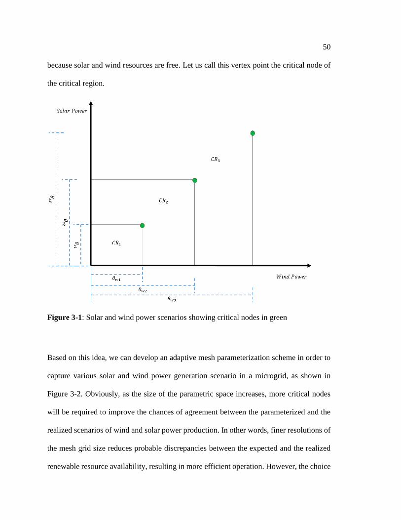
50

because solar and wind resources are free. Let us call this vertex point the critical node of

the critical region.

Figure 3-1: Solar and wind power scenarios showing critical nodes in green

Based on this idea, we can develop an adaptive mesh parameterization scheme in order to

capture various solar and wind power generation scenario in a microgrid, as shown in

Figure 3-2. Obviously, as the size of the parametric space increases, more critical nodes

will be required to improve the chances of agreement between the parameterized and the

realized scenarios of wind and solar power production. In other words, finer resolutions of

the mesh grid size reduces probable discrepancies between the expected and the realized

renewable resource availability, resulting in more efficient operation. However, the choice

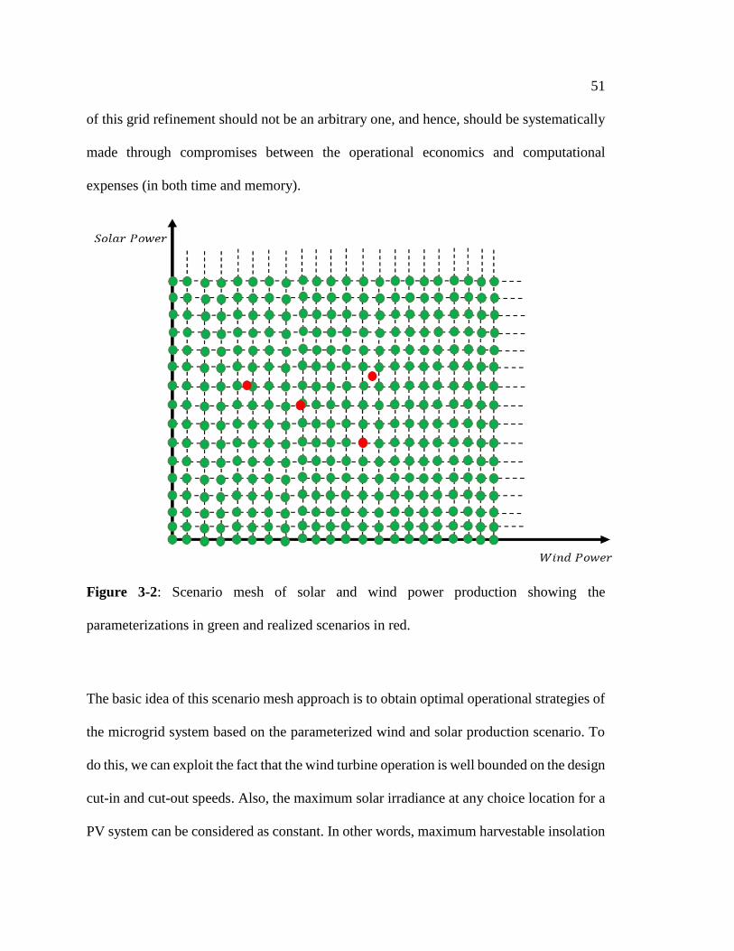
51

of this grid refinement should not be an arbitrary one, and hence, should be systematically

made through compromises between the operational economics and computational

expenses (in both time and memory).

Figure 3-2: Scenario mesh of solar and wind power production showing the

parameterizations in green and realized scenarios in red.

The basic idea of this scenario mesh approach is to obtain optimal operational strategies of

the microgrid system based on the parameterized wind and solar production scenario. To

do this, we can exploit the fact that the wind turbine operation is well bounded on the design

cut-in and cut-out speeds. Also, the maximum solar irradiance at any choice location for a

PV system can be considered as constant. In other words, maximum harvestable insolation

52

can be either limited by design or the upper limit of solar irradiation on earth – which is

reported to be about 1000 𝑊 𝑚2⁄ at standard conditions.

Optimization Objective Function

By parameterizing wind and solar power production potentials of the system into these

critical nodes, one can effectively formulate a set of state-space multiparametric

programming problems in the form of a bi-level optimization problem, the solution of

which can be expressed as explicit functions of the parameters. The problem can be solved

off-line and the results are mapped to the regions in the space of parameters where they are

valid. This provides a typical parametric profile which can be easily referenced for online

operational decision making.

Assuming a straight line depreciation model (equation 61) for the set of microgrid

technologies considered in this work. The bi-level optimization method is deployed to

minimize the net cost of the microgrid system. The outer problem in the formulation is

required to choose the right level of mesh grid refinement (resolution factor), while the

inner problem decides the right combinations of the system state variables to champion the

overall optimization objective.

min 𝑟𝑓

𝑍 = 𝐸𝜽𝑘∈𝑆{𝑄𝑘(𝜽)} (39)

𝑠. 𝑡.

𝑄𝑘(𝜽) = min𝒙𝑘∈𝑋,𝒚𝑘∈𝑌

𝑀𝑤,𝑘 +𝑀𝑠,𝑘 +𝑀𝑚,𝑘 +𝑀𝑢,𝑘 +𝑀𝑏,𝑘 (40)

𝑀𝑤,𝑘 = 𝑦𝑤,𝑘ℎ𝑤 + (𝑐𝑤 − 𝑒𝑤,𝑘)𝜃𝑤,𝑘 (41)

𝑀𝑠,𝑘 = 𝑦𝑠,𝑘ℎ𝑠 + (𝑐𝑠 − 𝑒𝑠,𝑘)𝜃𝑠,𝑘 (42)

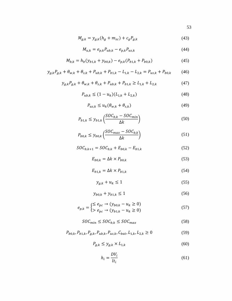
53

𝑀𝑔,𝑘 = 𝑦𝑔,𝑘(ℎ𝑔 +𝑚𝑠𝑐) + 𝑐𝑔𝑃𝑔,𝑘 (43)

𝑀𝑢,𝑘 = 𝑒𝑝,𝑘𝑃𝑢𝑏,𝑘 − 𝑒𝑝,𝑘𝑃𝑢𝑠,𝑘 (44)

𝑀𝑏,𝑘 = ℎ𝑏(𝑦𝑏1,𝑘 + 𝑦𝑏0,𝑘) − 𝑒𝑝,𝑘(𝑃𝑏1,𝑘 + 𝑃𝑏0,𝑘) (45)

𝑦𝑔,𝑘𝑃𝑔,𝑘 + 𝜃𝑤,𝑘 + 𝜃𝑠,𝑘 + 𝑃𝑢𝑏,𝑘 + 𝑃𝑏1,𝑘 − 𝐿1,𝑘 − 𝐿2,𝑘 = 𝑃𝑢𝑠,𝑘 + 𝑃𝑏0,𝑘 (46)

𝑦𝑔,𝑘𝑃𝑔,𝑘 + 𝜃𝑤,𝑘 + 𝜃𝑠,𝑘 + 𝑃𝑢𝑏,𝑘 + 𝑃𝑏1,𝑘 ≥ 𝐿1,𝑘 + 𝐿2,𝑘 (47)

𝑃𝑢𝑏,𝑘 ≤ (1 − 𝑢𝑘)(𝐿1,𝑘 + 𝐿2,𝑘) (48)

𝑃𝑢𝑠,𝑘 ≤ 𝑢𝑘(𝜃𝑤,𝑘 + 𝜃𝑠,𝑘) (49)

𝑃𝑏1,𝑘 ≤ 𝑦𝑏1,𝑘 (

𝑆𝑂𝐶𝑏,𝑘 − 𝑆𝑂𝐶𝑚𝑖𝑛∆𝑘

) (50)

𝑃𝑏0,𝑘 ≤ 𝑦𝑏0,𝑘 (

𝑆𝑂𝐶𝑚𝑎𝑥 − 𝑆𝑂𝐶𝑏,𝑘∆𝑘

) (51)

𝑆𝑂𝐶𝑏,𝑘+1 = 𝑆𝑂𝐶𝑏,𝑘 + 𝐸𝑏0,𝑘 − 𝐸𝑏1,𝑘 (52)

𝐸𝑏0,𝑘 = ∆𝑘 × 𝑃𝑏0,𝑘 (53)

𝐸𝑏1,𝑘 = ∆𝑘 × 𝑃𝑏1,𝑘 (54)

𝑦𝑔,𝑘 + 𝑢𝑘 ≤ 1 (55)

𝑦𝑏0,𝑘 + 𝑦𝑏1,𝑘 ≤ 1 (56)

𝑒𝑝,𝑘 = {

≤ 𝑒𝑝𝑐 → (𝑦𝑏0,𝑘 − 𝑢𝑘 ≥ 0)

> 𝑒𝑝𝑐 → (𝑦𝑏1,𝑘 − 𝑢𝑘 ≥ 0) (57)

𝑆𝑂𝐶𝑚𝑖𝑛 ≤ 𝑆𝑂𝐶𝑏,𝑘 ≤ 𝑆𝑂𝐶𝑚𝑎𝑥 (58)

𝑃𝑏0,𝑘, 𝑃𝑏1,𝑘, 𝑃𝑔,𝑘, 𝑃𝑢𝑏,𝑘 , 𝑃𝑢𝑠,𝑘, 𝐶𝑏𝑎𝑡, 𝐿1,𝑘, 𝐿2,𝑘 ≥ 0 (59)

𝑃𝑔,𝑘 ≤ 𝑦𝑔,𝑘 × 𝐿1,𝑘 (60)

ℎ𝑖 =

𝐷𝑉𝑖𝑙𝑡𝑖

(61)

54

𝑌 = {0,1}𝑖×𝑘

𝑃𝑖,𝑘,𝑀𝑖,𝑘 ∈ 𝑋

𝑘 = 1,… , 𝐾

The vector 𝒙 stands for the system state variables; 𝒚 is a vector of binary variables; and 𝜽

is the vector of parameters. Equations (39) and (40) are the outer and inner decision levels,

respectively; while (41) - (45) capture the net cost of the microgrid system components.

Individual elements of the cost are broken down in table 1 below. Equation (46) represents

the power balance requirement of the system, and (47) is a power constraint to ensure that

load demand is always satisfied. Equations (48) and (49) define the utility interaction rules

on how power could bought or sold to the main grid, with focus on ensuring that what is

sold is primarily renewable power. Equations (50) and (51) specify the battery discharge

and charge rate constraints, which forbid deep discharging and charging of the battery.

Equation (52) is the battery state of charge estimation equation, while (53) and (54) express

the battery charging and discharging energy respectively. Equation (55) is a constraint on

the microturbine to alleviate carbon emission by discouraging the system from selling

energy from the microturbine. Equation (56) is a prohibitive constraint to simultaneous

charging and discharging of the battery. Equation (57) is used to exploit the electricity spot

price dynamics to support selling excess power at high prices and storing it at low prices.

Equation (58) defines the battery state of charge limits. Equation (59) is a non-negativity

constraint on the system variables. Equation (60) recommends that in the event of

emergency islanding due to a possible breakdown of the main grid and loss of storage, the

microgrid is only required to satisfy the base/critical loads if the microturbine is activated.

Therefore, microturbine capacity is chosen based on the expected maximum critical load.

55

Table 3-1: Cost characteristics of the microgrid components

Component Depreciation (cents/h) Maintenance cost (cents/Wh) Lifetime (yrs)

WT 7.5 0.0008 20

MT 1.68 0.002 20

PV 18 0.0003 20

Battery 12 0.00015 1

Microturbine Startup and Shutdown Constraints

Constraints for minimum running and shutdown time are required to safeguard the lifetime

of the microturbine. Let 𝑁𝑜𝑛 and 𝑁𝑜𝑓𝑓 be sets that contain the running and shutdown states

(respectively) of the microturbine over the entire operational schedule. And two binary

variables, 𝑠𝑘 and 𝑟𝑘 denote the instantaneous deactivation and activation states of the MT

respectively; two other binary variables ��𝑘,𝑛 and ��𝑘,𝑛 capture the historical shutdown and

startup points; and the binary variable 𝑦𝑚,𝑘 represent the operating state of the MT during

the current interval 𝑘 ∈ 𝑇. Then, the following additional constraints can be established:

��𝑘+1,𝑛 = ��𝑘,𝑛−1 ∀ 𝑘 ∈ 𝑇, 𝑛 ∈ 𝑁𝑜𝑛: 𝑘 < 𝜏, 𝑛 > 0 (61)

��𝑘+1,𝑛 = ��𝑘,𝑛−1 ∀ 𝑘 ∈ 𝑇, 𝑛 ∈ 𝑁𝑜𝑓𝑓: 𝑘 < 𝜏, 𝑛 > 0 (62)

��𝑘,𝑛 = 𝑠𝑘 ∀ 𝑘 ∈ 𝑇, 𝑛 ∈ 𝑁𝑜𝑛: 𝜏𝑚𝑖𝑛

𝑜𝑛 ≥ 4, 𝑛 = 0 (63)

��𝑘,𝑛 = 𝑟𝑘 ∀ 𝑘 ∈ 𝑇, 𝑛 ∈ 𝑁𝑜𝑓𝑓: 𝜏𝑚𝑖𝑛

𝑜𝑓𝑓≥ 4, 𝑛 = 0 (645)

𝑟𝑘 − 𝑠𝑘 = 𝑦𝑚,𝑘 − 𝑦𝑚,𝑘−1 ∀ 𝑘 ∈ 𝑇 (656)

𝑦𝑚,𝑘 ≥ 𝑟𝑘 + ∑ ��𝑘,𝑛𝑛>0𝑛∈𝑁𝑜𝑛

∀ 𝑘 ∈ 𝑇: 𝜏𝑜𝑛 ≥ 4 (667)

56

1 − 𝑦𝑚,𝑘 ≥ 𝑠𝑘 + ∑ ��𝑘,𝑛𝑛>0

𝑛∈𝑁𝑜𝑓𝑓

∀ 𝑘 ∈ 𝑇: 𝜏𝑜𝑓𝑓 ≥ 4 (678)

The last two constraints define the minimum runtime and shutdown times of the

microturbine, respectively. Equations (62) and (63) are the difference equations for the

carryover variables that records an activation or deactivation events. Equations (64) and

(65) relates the carryover variables with their corresponding variables, while (66) relates

the startup and shutdown variables with the operating state variable.

A salient feature of the proposed approach is that the optimization is done off-line; since

wind and solar power production will fall within the range considered in the

multiparametric programming problem. Therefore, in the course of implementation, no

online optimization takes place, and the execution time of the MPP corresponds to the time

spent to identify the coordinates of the realized renewable resources. Solar power

production is calculated from equation (19), while wind turbine power output is obtained

using equations (22) and (23). Microturbine power level can be obtained from equations

(31) and (32). The simulation data are shown in table 2 below.

Table 3-2: Simulation parameters

cut in speed 3 m/s

cut out speed 25 m/s

rated speed 12 m/s

reference height 10 m

reference insolation 1000 W/m2

MT startup cost 20 cents

Min SOC limit 0.14

Max SOC limit 0.98

57

The problem which comprises of 240 binary variables and 360 continuous variables is

solved with CPLEX by interfacing GAMS 24.3.3 with MATLAB R2015a using an HP

Pavillion computer with Intel Core i7-3770 CPU 3.40 GHz and 8 GB RAM.

58

Results and Discussion

The results are organised by considering the effects of electricity pricing schemes and

energy storage conditions on the microgrid’s operational management decisions. Under

effects of pricing, both contract based and real-time price dynamics are considered. Actual

real-time pricing data which reflects a low price regime, and hypothetical pricing which

captures a high price regime are used. Two energy storage scenarios are incorporated to

represent small and large capacity storage systems. The small capacity storage is based on

the existing storage system in Lambton College, while the large storage mirrors a futuristic

storage arrangement.

4.1 Discussion of Results

Dynamic hourly electricity price (𝑒𝑝,𝑘) can be estimated from equation (36) and the

parameter, 𝑒𝑝𝑐 (threshold price), which is related to an estimate of the off-peak price, is

obtained from a time series of electricity price. Figure 4-1 shows electricity price profile in

Ontario over seven years, and a dashed red line is used to indicate the 𝑒𝑝𝑐 value. Based on

the analysis of the data, about 55% of the electricity prices fall between zero and the 𝑒𝑝𝑐

value. It can be observed that below that line, the price data is densely clustered, but above

the line it tends to distribute with less density. Above the threshold price, the system is

constrained to enforce discharging of stored energy. And below that price, the system is

required to prioritize its tasks by: supplying the load demand, charging the battery, and

then selling off any remaining power.

59

Figure 4-1: Electricity price profile for Ontario over a seven year period (courtesy of

Bluewater Power Corporation). The negative prices occur when power producers are

willing to pay in order to feed power into the network.

60

The parameterizations of the wind and solar power resources in form of a scenario mesh is

shown in Figure 4-2. Sequence of variations in the harnessed renewable on a winter day in

Sarnia, Ontario is highlighted, and it can be observed that this variability in the realized

renewable resources can be very severe; making it practically impossible to accurately

capture such transitions using any of the available meteorological modelling tools [12, 80].

However, with our modelling approach, the operational limits of the wind turbine and Solar

PV - as specified by system design – can be used to define the parametric space; which

decouples the solution of the energy management problem from weather prediction

accuracy. Besides, coarse meteorological predictions can be useful to tighten the

parametric space when they are proper subsets of the systems design space (which is the

case in this work). Under this situation, the optimality of the sequence of operational

decisions to be made might improve as a result of the higher chances of intersection

between the expected and the realized nodes. In any case, weather information is still

necessary to locate the current state of the microgrid system based on the prevailing

renewables realizations.

The resolution factor required to generate the scenario mesh is obtained by finding the best

trade-off between the average net cost and computational cost. Figure 4-3 shows the effect

of resolution factor on average net cost. The cost decreases appreciably at lower 𝑟𝑓 values,

and then levels off at around 𝑟𝑓 value of 50. Computational effort increases exponentially

over the range of 𝑟𝑓 values considered; as depicted by Figure 4-4. At the 𝑟𝑓 value of 50,

the scheduling problem requires a computational time of about 60 minutes. Hence, the

operational schedule can be recalculated - at the earliest - in the next hour when this 𝑟𝑓

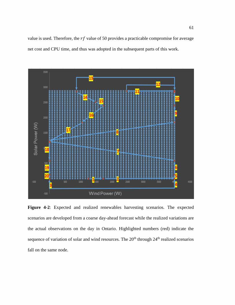
61

value is used. Therefore, the 𝑟𝑓 value of 50 provides a practicable compromise for average

net cost and CPU time, and thus was adopted in the subsequent parts of this work.

Figure 4-2: Expected and realized renewables harvesting scenarios. The expected

scenarios are developed from a coarse day-ahead forecast while the realized variations are

the actual observations on the day in Ontario. Highlighted numbers (red) indicate the

sequence of variation of solar and wind resources. The 20th through 24th realized scenarios

fall on the same node.

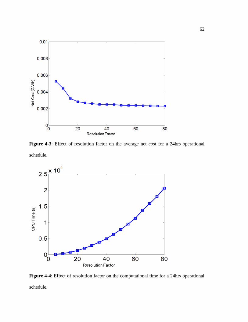
62

Figure 4-3: Effect of resolution factor on the average net cost for a 24hrs operational

schedule.

Figure 4-4: Effect of resolution factor on the computational time for a 24hrs operational

schedule.

63

Load profile of a residential building in Ontario on a typical winter day is used for the

simulations. Three realistic electricity pricing schemes – shown in Figure 4-5 – are

deployed in this work. Power production levels of the microgrid under the FIT and ETS

pricing systems are compared to the local load demand information in Figure 4-6.

Figure 4-5: Realistic pricing schemes based on Ontario data. FITs is for roof-top solar

while FITw is for onshore wind power. TOU is the time-of-use billing arrangement from

Bluewater Power. ETS is the real-time dynamic price.

64

The FIT pricing arrangement is based on Ontario’s Independent Electricity System

Operator micro-project fixed tariff contracts. ETS pricing is based on the dynamic real-

time electricity spot price through the electricity supply and demand bidding process. The

ETS pricing is applied to two energy storage scenarios: fixed capacity (ETSc) and

estimated capacity (ETSe). The fixed capacity storage is based on the given system design

constraint on the battery size, while the estimated capacity storage uses the electricity

pricing dynamics to recommend the right storage levels for best economic performance.

ETSe is enforced by redefining the maximum charging limit of the battery with a big-M

constraint. The real-time dynamic pricing data for the same winter day in consideration are

used for the ETS case studies. In the three cases displayed, the microgrid generates the

same amount of power over the 24hrs operational schedule. Also, the system is able to

satisfy all load demands over the schedule horizon.

Even though the load demand can be separated into critical and controllable loads, the

solution algorithm is constrained to satisfy both load classifications at all times.

Controllable loads consist of devices that are generally not required to be powered all the

time. Under such requirement, the load profile is developed using a demand-side

management scheme; which organizes the controllable load profile depending on when and

how the constituent devices will be needed or not. Here, 60% of the total load demand is

assumed to constitute the controllable load. The net electricity supply over demand is either

stored in the energy storage system or sold to the utility grid; depending on the economic

potential of each decision and/or constraint on storage capacity.

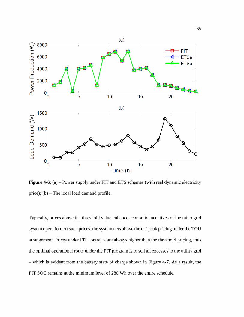
65

Figure 4-6: (a) – Power supply under FIT and ETS schemes (with real dynamic electricity

price); (b) – The local load demand profile.

Typically, prices above the threshold value enhance economic incentives of the microgrid

system operation. At such prices, the system nets above the off-peak pricing under the TOU

arrangement. Prices under FIT contracts are always higher than the threshold pricing, thus

the optimal operational route under the FIT program is to sell all excesses to the utility grid

– which is evident from the battery state of charge shown in Figure 4-7. As a result, the

FIT SOC remains at the minimum level of 280 Wh over the entire schedule.

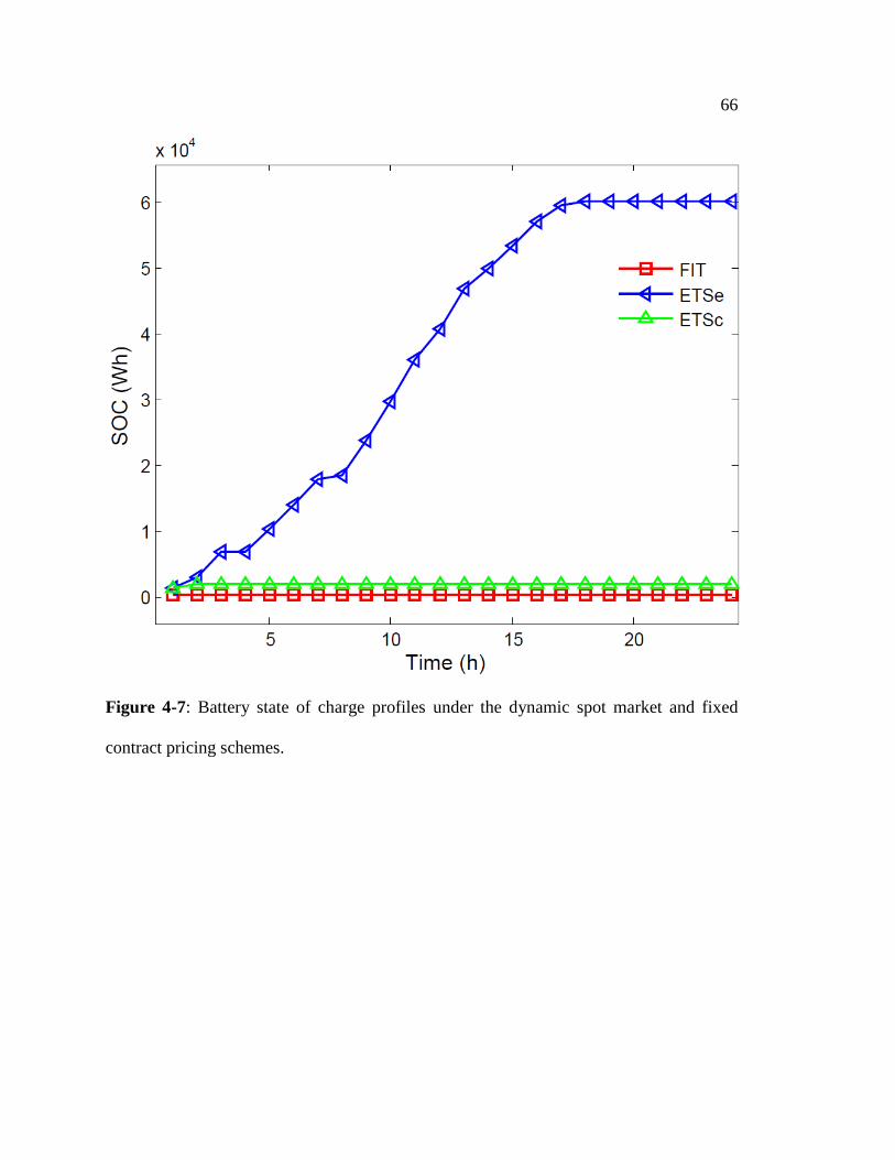
66

Figure 4-7: Battery state of charge profiles under the dynamic spot market and fixed

contract pricing schemes.

67

However, the situation is different for the two ETS cases. For ETSc, the SOC increases up

to the maximum charging limit of 1960 Wh; then all subsequent excess to load demand

have to be sold by the system regardless of the prevailing spot price. The SOC in the case

of ETSe suggests a smarter economic disposition by not selling power at prices below the

threshold price value. Instead, the energy management system continues to increases the

storage level by extending the charging limit until the eighteenth hour when there are no

renewables to be harvested, and the SOC saturates at about 60 kWh. Over the course of the

calculated schedule, the ETS prices are always below the 𝑒𝑝𝑐 value which makes it

unattractive to sell power to the grid, thereby requiring the microgrid to have a bigger

storage capacity. Obviously, longer simulation periods can be expected to expose the

system to the whole spectrum of variations in the electricity price.

In Figure 4-8, a hypothetical real-time ETS pricing scenario (P**) is created by increasing

the actual ETS price (P*) from the thirteenth hour, as shown in Figure 4-8(c), in order to

investigate the system behaviour during higher dynamic market prices. The modified price

values are applied to both the fixed capacity and the estimated capacity storage cases. As

the hypothetical ETS price is kept above the 𝑒𝑝𝑐 value, the energy management system

readjusts its recommended operational schedule to favour discharging of the storage system

in order to sell energy surpluses to the main grid. The large storage level of the ETSe

translates to the ability to leverage the economics of scale under favourable pricing

regimes. The limited storage allowance of the ETSc system has a restrictive influence on

the economic potentials of the microgrid even when electricity spot prices are very high.

In all cases, the minimum discharge limit constraints are enforced without violations.

68

Figure 4-8: Effect of pricing dynamics on battery state of charge; considering the actual

pricing (P*) and hypothetical pricing (P**) scenarios under the ETS system: (a) – state of

charge for the fixed capacity storage; (b) – state of charge for the estimated capacity

storage; (c) – dynamic real-time low and high electricity price scenarios.

69

In Figures 4-9 and 4-10, microgrid and main grid interaction allows power to be sold or

purchased both ways. The FIT scheme supports selling of all surplus renewable power

generation over load demand to the utility due to its subsidized tariff system. Whenever

renewable power production is inadequate for the residential load demand, the system buys

the shortfall of power through the utility grid connection. Under the actual ETS scheme,

the fixed capacity storage arrangement causes all renewable power surpluses to be sold to

the main grid once the storage limit has been attained, while the estimated capacity storage

does not encourage selling power to the main grid under the prevailing circumstances but

sends it to the storage. For the hypothetical ETS case, the higher electricity price trend

leads to discharge of the energy storage system in the two storage models.

Furthermore, with the actual ETS scheme, the energy management algorithm finds it to be

more economically beneficial to purchase power production deficits from the main grid,

due to the prevailing low electricity price; while conserving the renewable energy storage

for when prices will become more favourable. This decision has the additional advantage

of reducing the number of charge cycles of the battery during each operational schedule,

thereby improving the battery’s expected lifetime.

However, with the hypothetical ETS scheme, the energy management routine decides to

discharge some of the storage once the electricity price goes up. Subsequently, when the

dischargeable storage is depleted and the harvested renewable energy does not meet the

load demand, the algorithm activates the microturbine (as depicted in Figure 4-11); since

at high spot prices the microturbine’s operating and maintenance costs become competitive

despite the imposed emissions penalty. Accordingly, for the FIT and actual ETS pricing

schemes, the microturbine stays shutdown for the entire scheduling period.

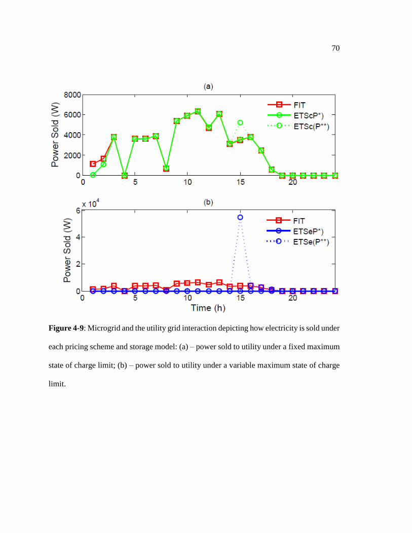
70

Figure 4-9: Microgrid and the utility grid interaction depicting how electricity is sold under

each pricing scheme and storage model: (a) – power sold to utility under a fixed maximum

state of charge limit; (b) – power sold to utility under a variable maximum state of charge

limit.

71

Figure 4-10: Microgrid and the main grid interaction displaying how power is bought from

the utility grid under each pricing scheme and storage model: (a) – power purchased from

utility under a fixed maximum state of charge limit; (b) – power purchased from utility

under a variable maximum state of charge limit.

72

Figure 4-11: Microturbine activation profile under the pricing schemes and storage

models. The microturbine remains shutdown for the low price regime ETS and the FIT

program. (a) – microturbine activation state under the fixed maximum state of charge limit.

(b) – microturbine activation state under the variable maximum state of charge limit.

73

In order to compare the economic performance of the operational decisions under the

considered pricing scenarios and storage models, results on the net costs for the FIT, the

actual ETS, and the hypothetical ETS are compared, along with the cost of meeting all load

demand by buying power completely from the utility (TOU), in Figure 4-12. Table 4-1

presents the overall net cost of the operational schedule for each of the considered pricing

schemes. It can be observed that the FIT program offers net financial benefits most of the

times, except during periods when there are no renewable resources to be harvested and

the load demand has to be purchased from the main grid.

Figure 4-12: Comparison of the net operating and maintenance cost of the microgrid under

various pricing scenarios and storage models, and the cost of purchasing all power demands

from the utility grid using the TOU pricing scheme.

74

Table 4-1: Comparing the cost of running a microgrid and that of relying on the utility.

Overall Net Cost ($)

FIT ETSc* ETSc** ETSe* ETSe** TOU

-13.34 0.68 0.17 3.46 -1.20 1.30

The real-time ETS pricing scheme provides net financial advantage during high prices if

the storage is big enough to offer some economics scale, but positive net costs during low

spot prices and when storage capacity is inadequate to provide significant economic

buffering effect on the costs. Therefore, it can be argued that the incorporation of adequate

battery energy storage system holds the promise for the economic viability of microgrid

projects under the electricity price bidding system. The storage system must be such that it

does not only enhance power quality by buffering power production deficits, but must also

exhibit some economic logic by leveraging the dynamic pricing environment of the ETS.

However, potential financial benefits of ETS-based projects should only be expected in the

long-run; as the occurrences of high and low electricity prices regimes tend to balance out.

75

Conclusions and Recommendations

5.1 Conclusions

Local power quality and environmental concerns associated with the conventional energy

systems have spurred a move towards an improved grid system consisting of distributed,

hybrid energy sources (renewable and non-renewable) and loads - a microgrid. In the face

of external uncertainties arising from electricity demand, price, and the availability of

renewable resources, the microgrid system is required to operate seamlessly and optimally

with or without interactions with a central grid network. To achieve this coordinated

operation requires sophisticated and efficient system-level integration and management of

the constituent energy systems in a microgrid. A major challenge is that renewable energy

is not dispatchable due to the apparent intermittency in the resource availability. Therefore,

managing this uncertainty in renewable resources is a critical hurdle before all hybrid

energy coordination algorithms - which are primarily optimization routines.

Generally, the varying parameters could be state variables and/or system parameters. In

our case, available solar and wind power are represented as the uncertain parameters.

Consequently, optimization problems involving parametric uncertainty can be

reformulated as multi-parametric programs, but the sacrifice with such transformation of

the problem is that it leads to time-based decomposition of the complete scheduling

problem. As a result, there may not be any theoretical guarantee of optimality or feasibility

of solutions; although the solutions are always bounds on the optimal solution of the

complete problem. Fortunately, long-term optimality is often not necessary or meaningful,

and feasibility can always be assured through tight constraints. Previously suggested

76

methods for handling this energy management problem have mostly been based on online

optimization techniques which suffer the handicap of weather forecasting errors,

dimensionality limitations, and unsuitable rate of system state transitions. These issues

manifest in the significant computational effort and cost demerits of the online methods.

This disquisition has proposed the multiparametric programming strategy as an algorithmic

improvement that makes efficient energy integration and management at the microgrid

level a realistic and practicable goal. For the purpose of this work, the MPP algorithm is

applied to a residential level microgrid project by considering case studies of electricity

pricing schemes based on incentivised feed-in contracts (FIT) and the open market price

bidding system (ETS). Effect of these pricing agreements on the optimal operational

scheduling of the microgrid is investigated by formulating the microgrid energy

management problem as a bi-level optimization problem that aims to minimize net cost of

the system operations. The linear structure of the formulation serves as a source of

confidence in the optimality of obtained solutions.

Under the FIT based arrangement, analysis of the results indicate that there is no

requirement for energy storage due to the financial benefits of selling power surpluses

through the main grid connection. Although the FIT program currently offers enticing

economic prospects, it is subject to change in the future since it is borne out of government

policy. When that happens, ETS based projects will have to leverage the open market

electricity price dynamics and battery energy storage systems in a structured approach in

order to be economically viable. Judging by the potential economic performances of the

77

case studies considered, it is observed that there is a compelling argument to consider a

microgrid project as against total dependence on the utility grid for all the domestic power

needs. By implication, the MPP method provides the right framework for assimilating

renewable energy systems into the present and future electric power sector by improving

uncertainty handling and reducing computational burden of the conventional methods.

In essence, the core merit of MPP is that it replaces the typical online optimization with

simple function evaluations (using wind speed and solar irradiance information to calculate

wind and solar power) that requires a smaller online computational effort in comparison

with online optimization. The concept of replacing online optimization through

deterministic mapping of optimal solutions enables “online optimization via off-line

optimization”. Thus, real-time implementation of the algorithm only involves

determination of the parametric coordinates in order to apply the relevant decisions,

without calls to an optimization solver.

5.2 Recommendations

Although realistic information on household load demand and electricity spot price has

been used in this study, future works can be expected to embed load and price forecasting

tools that enable real-time implementation of the proposed energy management technique.

Besides, demand-side management can be incorporated to capture the programming of

controllable and critical loads. Already, the nature of the MPP strategy makes this

realizable since one does not have to worry about the burden of accurate weather

78

prediction. Hence, there is room to accommodate the computational requirements of load

and price forecasting models.

Furthermore, longer periods of simulation will be needed to consolidate the confidence on

the potential economic performance of a microgrid project, and the application of parallel

computing can be of great use for extended runs of the energy management algorithm and

for incorporating forecasting algorithms into the overall energy management decision

making process.

79

BIBLIOGRAPHY

1. World Energy Outlook E. Statistics, Editor. 2014, International Energy Agency:

France.

2. Olivier, J.G.J., et al., Trends in Global CO2 Emissions, P.a.E.C.s.J.R. Centre,

Editor. 2014: The Hague.

3. Internaional Energy Outlook 2015, U.S.D.o. Energy, Editor. 2014: Washington D

C

4. El-Hawary, M.E., The Smart Grid-State-of-the-art and Future Trends. Electric

Power Components and Systems, 2014. 42(3-4): p. 239-250.

5. Prema, V. and K.U. Rao, Predictive Models For Power Management Of A Hybrid

Microgrid-A Review. Proceedings of the 2014 International Conference on

Advances in Energy Conversion Technologies (ICAECT): Intelligent Energy

Management: Technologies and Challenges, 2014: p. 7-12.

6. Liang, H. and W. Zhuang, Stochastic Modeling and Optimization in a Microgrid:

A Survey. Energies, 2014. 7(4): p. 2027-2050.

7. Bacha, S., et al., Photovoltaics in Microgrids. Ieee Industrial Electronics Magazine,

2015. 9(1): p. 33-46.

8. Olivares, D.E., et al., Trends in Microgrid Control. IEEE Transactions on Smart

Grid, 2014. 5(4): p. 1905-1919.

9. Mohammadi, S., et al, Optimal Operation Management of Microgrids Using the

Point Estimate Method and Firefly Algorithm While Considering Uncertainty.

Turkish Journal of Electrical Engineering and Computer Sciences, 2014. 22(3): p.

735-753.

10. Mahmoud, M.S., et al, Modeling and Control of Microgrid: An Overview. Journal

of the Franklin Institute-Engineering and Applied Mathematics, 2014. 351(5): p.

2822-2859.

11. Soshinskaya, M., et al., Microgrids: Experiences, Barriers and Success Factors.

Renewable & Sustainable Energy Reviews, 2014. 40: p. 659-672.

12. Liu, P., et al, An Energy Systems Engineering Approach for the Design and

Operation of Microgrids in Residential Applications. Chemical Engineering

Research and Design, 2013. 91(10): p. 2054-2069.

13. Camacho, E.F., et al., Control for Renewable Energy and Smart Grids. IEEE

Transactions on Control Systems Technology, 2012. 2: p. 1-20.

14. Chasaki, D. and N. Kondrath, Microgrids: Technical and Security

Recommendations for Future Implementations. 2014 IEEE International

Conference on Consumer Electronics (Icce), 2014: p. 315-316.

15. Callaway, D.W., et al., Time for a Revolution: Smart Energy and Microgrid Use in

Disaster Response. Disaster Medicine and Public Health Preparedness, 2014. 8(3):

p. 252-259.

16. Carpinelli, G., et al, Optimal Scheduling of a Microgrid with Demand Response

Resources. IET Generation Transmission & Distribution, 2014. 8(12): p. 1891-

1899.

80

17. Bozchalui, M.C., et al, Operation Strategies for Energy Storage Systems in

Distribution Networks. 2014 IEEE PES General Meeting - Conference &

Exposition, 2014.

18. Duong Tung, N. and L.B. Le, Risk-Constrained Profit Maximization for Microgrid

Aggregators with Demand Response. IEEE Transactions on Smart Grid, 2015. 6(1):

p. 135-146.

19. Eddy, Y.S.F., et al, Multi-Agent System for Distributed Management of Microgrids.

IEEE Transactions on Power Systems, 2015. 30(1): p. 24-34.

20. Zeng, B., et al., Environmental-Economic Dispatch for Smart Micro-Grid Using

Random Nelder Mead Optimized Shuffled Frog Leaf Algorithm. Journal of

Investigative Medicine, 2014. 62(8): p. S107-S107.

21. Wu, X., et al, A Hierarchical Framework for Generation Scheduling of Microgrids.

IEEE Transactions on Power Delivery, 2014. 29(6): p. 2448-2457.

22. Sechilariu, M., et al, Supervision Control for Optimal Energy Cost Management in

DC Microgrid: Design and Simulation. International Journal of Electrical Power &

Energy Systems, 2014. 58: p. 140-149.

23. Mazidi, M., et al., Integrated Scheduling of Renewable Generation and Demand

Response Programs in a Microgrid. Energy Conversion and Management, 2014.

86: p. 1118-1127.

24. Sercan, T., et al., Optimal Control of Battery Energy Storage for Wind Farm

Dispatching. IEEE Transactions on Energy Conversion, 2010. 25(3): p. 787-794.

25. Bracale, A., et al., Optimal Control Strategy of a DC Micro Grid. International

Journal of Electrical Power & Energy Systems, 2015. 67: p. 25-38.

26. Zhang, Y., et al., An Intelligent Control Strategy of Battery Energy Storage System

for Microgrid Energy Management under Forecast Uncertainties. International

Journal of Electrochemical Science, 2014. 9(8): p. 4190-4204.

27. Prodan, I. and E. Zio, A Model Predictive Control Framework for Reliable

Microgrid Energy Management. International Journal of Electrical Power &

Energy Systems, 2014. 61: p. 399-409.

28. Prodan, I. and E. Zio, Predictive Control for Reliable Microgrid Energy

Management Under Uncertainties. Safety, Reliability and Risk Analysis: Beyond

the Horizon, ed. R. Steenbergen, et al. 2014. 2919-2924.

29. Parisio, A., et al., Use of Model Predictive Control for Experimental Microgrid

Optimization. Applied Energy, 2014. 115: p. 37-46.

30. Barnes, A.K., et al, A Semi-Markov Model for Control of Energy Storage in Utility

Grids and Microgrids With PV Generation. IEEE Transactions on Sustainable

Energy, 2015. 6(2): p. 546-556.

31. Choudar, A., et al., A Local Energy Management of a Hybrid PV-Storage Based

Distributed Generation for Microgrids. Energy Conversion and Management,

2015. 90: p. 21-33.

32. Zou, S., et al, Auction-Based Distributed Efficient Economic Operations of

Microgrid Systems. International Journal of Control, 2014. 87(12): p. 2446-2462.

33. Sekhar, P.C., et al, Data analytics based neuro-fuzzy controller for diesel-

photovoltaic hybrid AC microgrid. IET Generation Transmission & Distribution,

2015. 9(2): p. 193-207.

81

34. Marinelli, M., et al., Testing of a Predictive Control Strategy for Balancing

Renewable Sources in a Microgrid. IEEE Transactions on Sustainable Energy,

2014. 5(4): p. 1426-1433.

35. Li, D. and S.K. Jayaweera, Distributed Smart-Home Decision-Making in a

Hierarchical Interactive Smart Grid Architecture. IEEE Transactions on Parallel

and Distributed Systems, 2015. 26(1): p. 75-84.

36. Biegler, L.T. and I.E. Grossmann, Retrospective on Optimization. Computers &

Chemical Engineering, 2004. 28(8): p. 1169-1192.

37. Sahinidis, N.V., Optimization Under Uncertainty: State-of-the-Art and

Opportunities. Computers & Chemical Engineering, 2004. 28(6-7): p. 971-983.

38. Li, X. and P.I. Barton, Optimal Design and Operation of Energy Systems Under

Uncertainty. Journal of Process Control, 2014.

39. Yazdanian, M. and A. Mehrizi-Sani, Distributed Control Techniques in

Microgrids. IEEE Transactions on Smart Grid, 2014. 5(6): p. 2901-2918.

40. Bouzid, A.M., et al., A Survey on Control of Electric Power Distributed Generation

Systems for Microgrid Applications. Renewable & Sustainable Energy Reviews,

2015. 44: p. 751-766.

41. Xu, X., et al., Hierarchical Energy Management System for Multi-Source Multi-

Product Microgrids. Renewable Energy, 2015. 78: p. 621-630.

42. Palizban, O. and K. Kauhaniemi, Hierarchical Control Structure in Microgrids

with Distributed Generation: Island and Grid-Connected Mode. Renewable &

Sustainable Energy Reviews, 2015. 44: p. 797-813.

43. Mao, M., et al., Multiagent-Based Hybrid Energy Management System for

Microgrids. IEEE Transactions on Sustainable Energy, 2014. 5(3): p. 938-946.

44. Soroush, M. and D.J. Chmielewski, Process Systems Opportunities in Power

Generation, Storage and Distribution. Computers & Chemical Engineering, 2013.

51: p. 86-95.

45. Kopanos, G.M. and E.N. Pistikopoulos, Reactive Scheduling by a Multiparametric

Programming Rolling Horizon Framework: A Case of a Network of Combined

Heat and Power Units. Industrial & Engineering Chemistry Research, 2014.

53(11): p. 4366-4386.

46. Silvente, J., et al., Reactive Scheduling for the Coordination of Energy Supply and

Demand Management in Microgrids, in 24th European Symposium on Computer

Aided Process Engineering, Pts a and B, J.J. Klemes, P.S. Varbanov, and P.Y.

Liew, Editors. 2014. p. 493-498.

47. Shayeghi, H. and B. Sobhani, Integrated Offering Strategy for Profit Enhancement

of Distributed Resources and Demand Response in Microgrids Considering System

Uncertainties. Energy Conversion and Management, 2014. 87: p. 765-777.

48. Shariatzadeh, F., et al., Real-Time Implementation of Intelligent Reconfiguration

Algorithm for Microgrid. IEEE Transactions on Sustainable Energy, 2014. 5(2): p.

598-607.

49. Papadaskalopoulos, D., et al, Decentralized Coordination of Microgrids With

Flexible Demand and Energy Storage. IEEE Transactions on Sustainable Energy,

2014. 5(4): p. 1406-1414.

82

50. Liu, N., et al., A Heuristic Operation Strategy for Commercial Building Microgrids

Containing EVs and PV System. IEEE Transactions on Industrial Electronics, 2015.

62(4): p. 2560-2570.

51. Wang, R., et al., Power Demand and Supply Management in Microgrids with

Uncertainties Of Renewable Energies. International Journal of Electrical Power &

Energy Systems, 2014. 63: p. 260-269.

52. Su, W., et al, Stochastic Energy Scheduling in Microgrids With Intermittent

Renewable Energy Resources. IEEE Transactions on Smart Grid, 2014. 5(4): p.

1876-1883.

53. Shi, L., et al, Bidding Strategy of Microgrid with Consideration of Uncertainty for

Participating in Power Market. International Journal of Electrical Power & Energy

Systems, 2014. 59: p. 1-13.

54. Wu, X., et al., Real-Time Energy Management Strategies for Microgrids. 2014

IEEE PEs General Meeting - Conference & Exposition, 2014.

55. Wu, H., et al, Dynamic Economic Dispatch of a Microgrid: Mathematical Models

and Solution Algorithm. International Journal of Electrical Power & Energy

Systems, 2014. 63: p. 336-346.

56. Provata, E., et al., Development of Optimization Algorithms for the Leaf Community

Microgrid. Renewable Energy, 2015. 74: p. 782-795.

57. Elrayyah, A., et al, A Novel Load-Flow Analysis for Stable and Optimized

Microgrid Operation. IEEE Transactions on Power Delivery, 2014. 29(4): p. 1709-

1717.

58. Nejad, R.R. and S.M.M. Tafreshi, Operation Planning of a Smart Microgrid

Including Controllable Loads and Intermittent Energy Resources by Considering

Uncertainties. Arabian Journal for Science and Engineering, 2014. 39(8): p. 6297-

6315.

59. Moradi, M.H. and M. Eskandari, A Hybrid Method for Simultaneous Optimization

of DG Capacity and Operational Strategy in Microgrids Considering Uncertainty

in Electricity Price Forecasting. Renewable Energy, 2014. 68: p. 697-714.

60. Litchy, A.J., et al, Real-Time Energy Management of an Islanded Microgrid Using

Multi-Objective Particle Swarm Optimization. 2014 IEEE PES General Meeting -

Conference & Exposition, 2014.

61. Olivares, D.E., et al, A Centralized Energy Management System for Isolated

Microgrids. IEEE Transactions on Smart Grid, 2014. 5(4): p. 1864-1875.

62. Mantovani, G., et al., Experimental Validation of Energy Resources Integration in

Microgrids via Distributed Predictive Control. IEEE Transactions on Energy

Conversion, 2014. 29(4): p. 1018-1025.

63. Marietta, M.P., et al, A Rolling Horizon Rescheduling Strategy for Flexible Energy

in a Microgrid. 2014 IEEE International Energy Conference (Energycon 2014),

2014: p. 1297-1303.

64. Malysz, P., et al, An Optimal Energy Storage Control Strategy for Grid-connected

Microgrids. IEEE Transactions on Smart Grid, 2014. 5(4): p. 1785-1796.

65. Li, P., et al., Probabilistic Optimal Operation Management of Microgrid Using

Point Estimate Method and Improved Bat Algorithm. 2014 IEEE PES General

Meeting - Conference & Exposition, 2014.

83

66. Elsied, M., et al., An Advanced Energy Management of Microgrid System Based on

Genetic Algorithm. 2014 Ieee 23rd International Symposium on Industrial

Electronics (Isie), 2014: p. 2541-2547.

67. Bjelic, I.B. and R.M. Ciric, Optimal Distributed Generation Planning at a Local

Level - A Review of Serbian Renewable Energy Development. Renewable &

Sustainable Energy Reviews, 2014. 39: p. 79-86.

68. Shadmand, M.B. and R.S. Balog, Multi-Objective Optimization and Design of

Photovoltaic-Wind Hybrid System for Community Smart DC Microgrid. IEEE

Transactions on Smart Grid, 2014. 5(5): p. 2635-2643.

69. Xu, Y. and Z. Li, Distributed Optimal Resource Management Based on the

Consensus Algorithm in a Microgrid. IEEE Transactions on Industrial Electronics,

2015. 62(4): p. 2584-2592.

70. Chakraborty, S., et al, Real-Time Energy Exchange Strategy of Optimally

Cooperative Microgrids for Scale-Flexible Distribution System. Expert Systems

with Applications, 2015. 42(10): p. 4643-4652.

71. Ou, T.-C. and C.-M. Hong, Dynamic Operation and Control of Microgrid Hybrid

Power Systems. Energy, 2014. 66: p. 314-323.

72. Lei, X., et al., An Optimal Purchase and Sale Power Model Considering

Microgrids. International Transactions on Electrical Energy Systems, 2015. 25(2):

p. 246-261.

73. Pistikopoulos, E.N., et al., Theoretical and Algorithmic Advances in Multi-

Parametric Programming and Control. Computational Management Science,

2012. 9(2): p. 183-203.

74. Parisio, A., et al, A Model Predictive Control Approach to Microgrid Operation

Optimization. IEEE Transactions on Control Systems Technology, 2014. 22(5): p.

1813-1827.

75. Biyik, E. and R. Chandra, Optimal Control of Microgrids - Algorithms and Field

Implementation. 2014 American Control Conference (Acc), 2014: p. 5003-5009.

76. Farzan, F., et al., Toward Optimal Day-Ahead Scheduling and Operation Control

of Microgrids Under Uncertainty. IEEE Transactions on Smart Grid, 2015. 6(2): p.

499-507.

77. Caldognetto, T., et al., Improving Microgrid Performance by Cooperative Control

of Distributed Energy Sources. IEEE Transactions on Industry Applications, 2014.

50(6): p. 3921-3930.

78. Deckmyn, C., et al., Multi-Objective Optimization for Environomic Scheduling in

Microgrids. 2014 IEEE PES General Meeting - Conference & Exposition, 2014.

79. Rahbar, K., et al., An Off-Line Optimization Approach for Online Energy Storage

Management in Microgrid System. 2014 IEEE International Conference on

Acoustics, Speech and Signal Processing (Icassp), 2014.

80. Wang, X., et al., An Economic Receding Horizon Optimization Approach for

Energy Management in the Chlor-Alkali Process with Hybrid Renewable Energy

Generation. Journal of Process Control, 2014. 24(8): p. 1318-1327.

81. Trifkovic, M., et al., Dynamic Real-Time Optimization and Control of a Hybrid

Energy System. AIChE Journal, 2014. 60(7): p. 2546-2556.

84

82. Trifkovic, M., et al., Modeling and Control of a Renewable Hybrid Energy System

With Hydrogen Storage. IEEE Transactions On Control Systems Technology,

2014. 22(1): p. 169-179.

83. Ulbig, A., et al., Framework for Multiple Time-Scale Cascaded MPC Application

in Power Systems, in International Federation of Automatic Control. 2011: Milano.

84. Fossati, J.P., et al., Optimal Scheduling of a Microgrid with a Fuzzy Logic

Controlled Storage System. International Journal of Electrical Power & Energy

Systems, 2015. 68: p. 61-70.

85. Pinceti, P., et al., Design Criteria for a Power Management System for Microgrids

with Renewable Sources. Electric Power Systems Research, 2015. 122: p. 168-179.

86. Pan, I. and S. Das, Kriging Based Surrogate Modeling for Fractional Order

Control of Microgrids. IEEE Transactions on Smart Grid, 2015. 6(1): p. 36-44.

87. Kuznetsova, E., et al., Analysis of Robust Optimization for Decentralized Microgrid

Energy Management Under Uncertainty. International Journal of Electrical Power

& Energy Systems, 2015. 64: p. 815-832.

88. Hu, M.-C., et al., Optimal Operating Strategies and Management for Smart

Microgrid Systems. Journal of Energy Engineering, 2014. 140(1).

89. Hittinger, E., et al., Evaluating the Value of Batteries in Microgrid Electricity

Systems using an Improved Energy Systems Model. Energy Conversion and

Management, 2015. 89: p. 458-472.

90. Faber, I., et al., Micro-Energy Markets: The Role of a Consumer Preference Pricing

Strategy on Microgrid Energy Investment. Energy, 2014. 74: p. 567-575.

91. Alam, M.R., et al., A Modular Framework for Cost Optimization in Smart Grid.

2014 IEEE World Forum on Internet of Things (Wf-Iot), 2014: p. 337-340.

92. Li, X., et al., A Hierarchical Energy Management Strategy for Grid-connected

Microgrid. 2014 IEEE PES General Meeting - Conference & Exposition, 2014.

93. Collazos, A., et al, Predictive Optimal Management Method for the Control of

Polygeneration Systems. Computers & Chemical Engineering, 2009. 33(10): p.

1584-1592.

94. Fathima, A.H. and K. Palanisamy, Optimization in Microgrids with Hybrid Energy

Systems - A Review. Renewable & Sustainable Energy Reviews, 2015. 45: p. 431-

446.

95. Toma, P., et al., Sizing Photovoltaic-Wind Smart Microgrid with Battery Storage

and Grid Connection. 2014 IEEE International Conference on Automation, Quality

and Testing, Robotics, 2014.

96. Zachar, M., et al, Policy Effects on Microgrid Economics, Technology Selection,

and Environmental Impact. Computers & Chemical Engineering, 2015.

97. Fossati, J.P., et al., A Method for Optimal Sizing Energy Storage Systems for

Microgrids. Renewable Energy, 2015. 77: p. 539-549.

98. Lawder, M.T., et al, Balancing Autonomy and Utilization of Solar Power and

Battery Storage for Demand Based Microgrids. Journal of Power Sources, 2015.

279: p. 645-655.

99. Ramadesigan, V., et al., Modeling and Simulation of Lithium-Ion Batteries from a

Systems Engineering Perspective. Journal of the Electrochemical Society, 2012.

159(3): p. R31-R45.

85

100. Prasad, A. and E. Natarajan, Optimization of Integrated Photovoltaic–Wind Power

Generation Systems with Battery Storage. Energy, 2006. 31(12): p. 1943-1954.

101. Lv, X., et al., TOU Optimization Model of Microgrid Based on Demand Side

Response and Economical Operation. Proceedings of the 2014 International

Conference on Mechatronics, Electronic, Industrial and Control Engineering, 2014.

5: p. 71-76.

102. Zhou, K., et al., Optimal Load Distribution Model of Microgrid in the Smart Grid

Environment. Renewable & Sustainable Energy Reviews, 2014. 35: p. 304-310.

103. Hanmandlu, M.C., et al, Load Forecasting Using Hybrid Models. Power Systems,

IEEE Transactions, 2011. 26(1): p. 20-29.

104. Rong, W.M. et al, Design of Time-of-Use Power Price at Generation Side and

Optimal Model of Electricity Distribution Electric Power Automation Equipment,

2007. 27(8): p. 16-21.

105. Jian-bao., et al, Optimization Model for Designing Peak-Valley Time-Of-Use

Power Price of Generation Side and Sale Side at the Direction of Energy

Conservation Dispatch Zhongguo dianji gongcheng xuebao 2009. 29(1): p. 55-62.

106. Ruan, W.W., et al, Customer Response Behavior in Time-of-Use Price. Dianwang

jishu, 2012. 36(7): p. 86-93.

107. Liu, Y., Research on TOU Rate Design Optimization Model Chinese Journal of

Management Science 2005. 13(5): p. 87-92.

108. Oldewurtel, F., et al., Building Control and Storage Management with Dynamic

Tariffs for Shaping Demand Response, in Innovative Smart Grid Technologies -

IEEE PES International Conference and Exhibition. 2011, IEEE Conference

Publications: Manchester. p. 1 - 8.

109. Ulbig, A. and G. Andersson, Towards Variable End-Consumer Electricity Tariffs

Reflecting Marginal Costs: A Benchmark Tariff in IEEE EEM 2010 Conference.

2010, IEEE: Madrid. p. 1-6.

110. Shirazi, E. and S. Jadid, Optimal Residential Appliance Scheduling Under Dynamic

Pricing Scheme via HEMDAS. Energy and Buildings, 2015. 93: p. 40-49.

111. Wang, K., et al, Load Scheduling Strategies Based on Dynamic Price in Smart

Grid, in Energy Development, Pts 1-4, Q. Xu, Y. Li, and X. Yang, Editors. 2014.

p. 2495-2500.

112. Liu, Y., et al., Electricity Cost Minimization for a Microgrid With Distributed

Energy Resource Under Different Information Availability. IEEE Transactions on

Industrial Electronics, 2015. 62(4): p. 2571-2583.

113. Hu, C., et al., Energy Coordinative Optimization of Wind-Storage-Load Microgrids

Based on Short-Term Prediction. Energies, 2015. 8(2): p. 1505-1528.

114. Lim, Y. and H.-M. Kim, Strategic Bidding Using Reinforcement Learning for Load

Shedding in Microgrids. Computers & Electrical Engineering, 2014. 40(5): p.

1439-1446.

115. Janik, P., et al., Potentials of Microgrids - RES infeed, stationary storage and

controllable loads modelling. 2014 IEEE 16th International Conference on

Harmonics and Quality of Power (Ichqp), 2014: p. 655-658.

116. Goyal, M., et al., Overload Prevention in an Autonomous Microgrid using Battery

Storage Units. 2014 IEEE PES General Meeting - Conference & Exposition, 2014.

86

117. Fabisz, K., et al., Profiling of Prosumers for the Needs of Energy Demand

Estimation in Microgrids. 2014 5th International Renewable Energy Congress

(Irec), 2014.

118. Saez, D., et al., Fuzzy Prediction Interval Models for Forecasting Renewable

Resources and Loads in Microgrids. IEEE Transactions on Smart Grid, 2015. 6(2):

p. 548-556.

119. Hernandez, L., et al., Artificial Neural Networks for Short-Term Load Forecasting

in Microgrids Environment. Energy, 2014. 75: p. 252-264.

120. Lachowicz., T.S., et al, Tuning Fuzzy Systems to Achieve Economic Dispatch for

Microgrids, in 2011 IEEE Innovative Smart Grid Technologies Asia. 2011, IEEE:

Perth, Australia. p. 1-6.

121. Acevedo, J. and E. Pistikopoulos, A Multiparametric Programming Approach for

Linear Process Engineering Problems under Uncertainty. Industrial & Engineering

Chemistry Research, 1997. 36: p. 717-728.

122. Dua, V., et al, A Multiparametric Programming Approach for Mixed-Integer

Quadratic Engineering Problems. Computers & Chemical Engineering, 2002. 26:

p. 715-733.

123. Tenfen, D. and E.C. Finardi, A Mixed Integer Linear Programming Model for the

Energy Management Problem of Microgrids. Electric Power Systems Research,

2015. 122: p. 19-28.

124. Sechilariu, M., et al., Power Management and Optimization for Isolated DC

Microgrid. 2014 International Symposium on Power Electronics, Electrical Drives,

Automation and Motion (Speedam), 2014: p. 1284-1289.

125. Dua, V. and E. Pistikopoulo, An Algorithm for the Solution of Multiparametric

Mixed Integer Linear Programming Problems. Anals of Operations Research,

2000. 99: p. 123-139.

87

Appendices

All additional data used in this work are provided under this section. Each entry is identified

alphabetically and the sources of information are duly acknowledged.

Appendix A: Time-of-use (TOU) electricity cost

Appendix B.1: FIT price adders for all FIT project sizes and all renewables (courtesy of

Independent Electricity System Operator, Ontario).

88

Appendix B.2: Feed-in tariff price schedule (courtesy of Independent Electricity System

Operator, Ontario. Projects with Nameplate Capacity of 10kW or less are known as

microFIT, while those that are above 10kW are categorized under the FIT program).