The Pennsylvania State University

The Graduate School

Department of Industrial and Manufacturing Engineering

MULTI-OBJECTIVE, INTEGRATED SUPPLY CHAIN

DESIGN AND OPERATION UNDER UNCERTAINTY

A Dissertation in

Industrial Engineering and Operations Research

by

Christopher James Solo

2009 Christopher James Solo

Submitted in Partial Fulfillment of the Requirements

for the Degree of

Doctor of Philosophy

August 2009

The dissertation of Christopher James Solo was reviewed and approved* by the following:

A. Ravindran Professor of Industrial Engineering and Affiliate Professor of IST School Industrial and Manufacturing Engineering Dissertation Advisor Chair of Committee

Soundar R.T. Kumara Allen E. Pearce/Allen M. Pearce Chaired Professor Industrial and Manufacturing Engineering

M. Jeya Chandra Professor of Industrial and Manufacturing Engineering Industrial and Manufacturing Engineering

Susan H. Xu Professor of Management Science and Supply Chain Management Supply Chain and Information Systems

A. Ravindran Interim Department Head Industrial and Manufacturing Engineering

*Signatures are on file in the Graduate School

iii

ABSTRACT

This research involves the development of a flexible, multi-objective optimization

tool for use by supply chain managers in the design and operation of manufacturing-

distribution networks under uncertain demand conditions. The problem under

consideration consists of determining the supply chain infrastructure; raw material

purchases, shipments, and inventories; and finished product production quantities,

inventories, and shipments needed to achieve maximum profit while fulfilling demand

and minimizing supply chain response time. The development of the two-phase

mathematical model parallels the supply chain planning process through the formulation

of a strategic submodel for infrastructure design followed by a tactical submodel for

operational planning. The deterministic strategic submodel, formulated as a multi-period,

mixed integer linear programming model, considers an aggregate production planning

problem in which long-term decisions such as plant construction, production capacities,

and critical raw material supplier selections are optimized. These decisions are then used

as inputs in the operational planning portion of the problem. The deterministic tactical

submodel, formulated as a multi-period, mixed integer linear goal programming model,

uses higher resolution demand and cost data, newly acquired transit time information, and

the previously developed infrastructure to determine optimal non-critical raw material

supplier selections; revised purchasing, production, inventory, and shipment quantities;

and an optimal profit figure. The supply chain scenario is then modified to consider

uncertain, long-term demand forecasts in the form of discrete economic scenarios. In this

case, a multi-period, mixed integer robust optimization formulation of the strategic

iv

submodel is presented to account for the probabilistic demand data. Once the stochastic

strategic submodel is presented, short-term, uncertain demand data is assumed to be

available in the form of continuous probability distributions. By modifying decision

makers’ objectives regarding demand satisfaction, the distribution-based demand data is

accounted for through the development of a multi-period, mixed integer chance-

constrained goal programming formulation of the tactical submodel. In order to

demonstrate the flexibility of both the deterministic and stochastic versions of the overall

two-phase model, numerical examples are presented and solved. The resulting work

provides supply chain managers with a flexible tool that can aid in the design and

operation of real-world production-distribution networks, where uncertain demand data is

available at different times and in various forms.

v

TABLE OF CONTENTS

Chapter 1 INTRODUCTION, MOTIVATION, AND PROBLEM STATEMENT ...1

Chapter 2 LITERATURE REVIEW ...........................................................................13

2.1 Multi-echelon supply chain modeling.............................................................14 2.2 Multi-objective deterministic supply chain modeling ....................................16

2.2.1 Deterministic supply chain optimization using goal programming......19 2.3 Supplier selection techniques..........................................................................20 2.4 Handling uncertainty in supply chain problems .............................................22

2.4.1 Robust optimization for supply chain problems under uncertainty......24 2.4.2 Stochastic goal programming for supply chain problems under

uncertainty ..............................................................................................29 2.6 Summary .........................................................................................................33

Chapter 3 SINGLE PRODUCT, MULTI-OBJECTIVE, DETERMINISTIC SUPPLY CHAIN MODEL...................................................................................35

3.1 Problem and model overview .........................................................................35 3.2 Notation...........................................................................................................39 3.3 Strategic submodel..........................................................................................41

3.3.1 Strategic submodel objective function..................................................43 3.3.1.1 Plant construction costs ..............................................................44 3.3.1.2 Fixed operating costs for plants and warehouses .......................44 3.3.1.3 Raw material costs......................................................................45 3.3.1.4 Variable production costs ...........................................................46 3.3.1.5 Production quantity change costs ...............................................47 3.3.1.6 Shipping costs for raw materials and finished products .............48 3.3.1.7 Holding costs for raw materials / finished products at plants

and warehouses................................................................................49 3.3.2 Strategic submodel constraints .............................................................50

3.3.2.1 Raw materials supplier selection and availability ......................50 3.3.2.2 Plant construction decisions .......................................................52 3.3.2.3 Plant capacity..............................................................................52 3.3.2.4 Production quantity changes.......................................................53 3.3.2.5 Plant flow conservation (raw materials) .....................................53 3.3.2.6 Plant raw material storage capacity ............................................54 3.3.2.7 Plant flow conservation (finished products) ...............................55 3.3.2.8 Plant finished product storage capacity ......................................55 3.3.2.9 Warehouse flow conservation (finished products) .....................56 3.3.2.10 Warehouse capacity and selections ..........................................57 3.3.2.11 Ending inventory requirement ..................................................58 3.3.2.12 Demand.....................................................................................58

3.3.3 Strategic submodel summary................................................................61

vi

3.4 Tactical submodel ...........................................................................................62 3.4.1 Additional notation ...............................................................................65 3.4.2 Tactical submodel goal constraints.......................................................66

3.4.2.1 Profit optimization goal constraint .............................................66 3.4.2.2 Construction costs.......................................................................67 3.4.2.3 Fixed operating costs for plants and warehouses .......................68 3.4.2.4 Raw material costs......................................................................68 3.4.2.5 Variable production costs ...........................................................69 3.4.2.6 Production quantity change costs ...............................................69 3.4.2.7 Shipping costs for raw materials and finished products .............69 3.4.2.8 Holding costs for raw materials / finished products at plants

and warehouses................................................................................70 3.4.3 Total weighted transit time goal constraint...........................................71 3.4.4 Customer demand non-traditional goal constraint................................72 3.4.5 Tactical submodel regular constraints ..................................................73

3.4.5.1 Raw materials supplier selection and availability ......................73 3.4.5.2 Production capacity ....................................................................75 3.4.5.3 Production quantity changes.......................................................76 3.4.5.4 Plant flow conservation (raw materials) .....................................77 3.4.5.5 Plant raw material storage capacity ............................................77 3.4.5.6 Plant flow conservation (finished products) ...............................78 3.4.5.7 Plant finished product storage capacity ......................................78 3.4.5.8 Warehouse flow conservation (finished products) .....................79 3.4.5.9 Warehouse capacity....................................................................80 3.4.5.10 Ending inventory requirement ..................................................81

3.4.6 Tactical submodel objective function ...................................................81 3.4.7 Tactical submodel summary .................................................................86

3.5 Numerical example .........................................................................................87 3.5.1 Input data ..............................................................................................89 3.5.2 Preemptive goal programming solution technique ...............................92 3.5.3 Results...................................................................................................93

3.6 Deterministic model summary ........................................................................100

Chapter 4 SCENARIO-BASED, MULTI-OBJECTIVE, STOCHASTIC STRATEGIC SUBMODEL........................................................102

4.1 Introduction.....................................................................................................102 4.2 Stochastic optimization review .......................................................................104 4.3 Robust optimization review ............................................................................106 4.4 Notation...........................................................................................................111 4.5 Constraints ......................................................................................................114

4.5.1 Warehouse flow conservation (finished products) ...............................114 4.5.2 Warehouse capacity and selections.......................................................115 4.5.3 Ending inventory requirement ..............................................................116 4.5.4 Customer demand non-traditional goal constraint................................116

vii

4.6 Objective function formulation.......................................................................117 4.6.1 Profit terms ...........................................................................................118

4.6.1.1 Shipping costs for raw materials and finished products ............119 4.6.1.2 Holding costs for raw materials / finished products at plants

and warehouses................................................................................120 4.6.1.3 Expected total profit ...................................................................121 4.6.1.4 Weighted profit variance term....................................................121

4.6.2 Infeasibility penalty term ......................................................................122 4.6.3 Overall objective function formulation.................................................123

4.7 Overall formulation.........................................................................................124 4.8 Numerical example .........................................................................................127

4.8.1 Input data ..............................................................................................128 4.8.2 Results...................................................................................................129 4.8.3 Comparison with the deterministic strategic submodel solution ..........132

4.9 Stochastic strategic submodel summary .........................................................135

Chapter 5 DISTRIBUTION-BASED, MULTI-OBJECTIVE, STOCHASTIC TACTICAL SUBMODEL ..........................................................137

5.1 Introduction.....................................................................................................137 5.2 Chance-constrained goal programming review ..............................................139 5.3 Notation...........................................................................................................142 5.4 Goal constraints...............................................................................................143

5.4.1 Customer demand goal constraint.........................................................144 5.4.2 Profit optimization goal constraint .......................................................149 5.4.3 Total weighted transit time goal constraint...........................................150

5.5 Ending inventory chance constraint ................................................................150 5.6 Regular constraints..........................................................................................154 5.7 Objective function and overall formulation ....................................................154 5.8 Numerical example .........................................................................................157

5.8.1 Input data ..............................................................................................158 5.8.2 Results...................................................................................................163

5.9 Stochastic tactical submodel summary ...........................................................170

Chapter 6 CONCLUSIONS AND FUTURE WORK.................................................172

6.1 Summary .........................................................................................................172 6.2 Future research................................................................................................176

Bibliography.................................................................................................................179

viii

LIST OF FIGURES

Figure 1-1: Notional supply chain configuration. ........................................................4

Figure 3-1: Inputs and outputs of strategic and tactical submodels. ............................38

Figure 3-2: Example supply chain scenario. ................................................................88

Figure 3-3: Profit goal achievement as a percentage of goal target. ............................97

Figure 3-4: Demand goal achievement as a percentage of goal target........................99

Figure 4-1: Total demand satisfaction by scenario and market. ..................................131

Figure 4-2: Tradeoff between expected total profit and expected unsatisfied demand. .................................................................................................................132

Figure 5-1: Standard normal plot for demand chance constraint. ................................146

Figure 5-2: Standard normal plot for ending inventory chance constraint. .................153

Figure 5-3: Profit goal achievement as a percentage of goal target. ............................165

Figure 5-4: Notional demand goal achievement as a percentage of goal target. .........166

ix

LIST OF TABLES

Table 2-1: Multi-objective and stochastic characteristics of selected supply chain papers. ...................................................................................................................33

Table 3-1: Strategic submodel cost ranges...................................................................90

Table 3-2: Plant costs and capacities............................................................................90

Table 3-3: Warehouse costs and capacities..................................................................91

Table 3-4: Market demand (units)................................................................................91

Table 3-5: Numerical example model size (profit first)...............................................93

Table 3-6: Critical raw material supplier selections.....................................................94

Table 3-7: Warehouse operating schedule. ..................................................................94

Table 3-8: Strategic submodel optimal production quantities. ....................................95

Table 3-9: Tactical submodel production capacities....................................................95

Table 3-10: Tactical submodel optimal production (profit first). ................................96

Table 3-11: Tactical submodel optimal production (demand first)..............................97

Table 3-12: Production change as demand goal replaces profit goal as top priority. ..98

Table 3-13: Demand shortages (profit first/demand first.) ..........................................99

Table 4-1: Market demand (units)................................................................................128

Table 4-2: Critical raw material supplier selections.....................................................129

Table 4-3: Warehouse operating schedule. ..................................................................129

Table 4-4: Stochastic strategic submodel optimal production quantities.....................130

Table 4-5: Stochastic strategic submodel demand shortages. ......................................130

Table 4-6: Shortages/excess deliveries relative to stochastic demand.........................133

Table 5-1: Market demand (units)................................................................................159

Table 5-2: Confidence levels for meeting demand (chance-constrained goals.) .........160

x

Table 5-3: Tactical submodel production capacities....................................................162

Table 5-4: Numerical example model size (profit first)...............................................163

Table 5-5: Tactical submodel optimal production (profit first). ..................................164

Table 5-6: Tactical submodel optimal production (demand first)...............................165

Table 5-7: Demand shortages (profit first/demand first.) ............................................167

Table 5-8: Actual probabilities of meeting demand goals. ..........................................169

xi

ACKNOWLEDGMENTS

Penn State’s legendary football coach Joe Paterno once said, “Believe deep down

in your heart that you’re destined to do great things.” Such confidence in one’s own self,

coupled with guidance from those who have gone before you and the support of those

who go alongside you, can indeed lead to great things. A few words can hardly express

my gratitude to those people who made this accomplishment possible. First, I thank

those who have travelled this road before me. Without the guiding wisdom and academic

expertise of my research advisor, Dr. A. Ravi Ravindran, along with the insightfulness

and support of the research committee members, I am certain I would have lacked the

knowledge and focus necessary to successfully complete this research. Next, I thank

those who travelled this road alongside me. Enduring the late nights, odd schedule, and

(surely) uninteresting dinner conversations regarding coding errors and formulation

difficulties, my wife and children provided more support and encouragement than I could

have ever hoped for. I am truly humbled by the selflessness and love they’ve shown

throughout this adventure. Thank you—Susie, Michael, and Molly—for helping me

believe in myself and achieve a great thing.

Christopher J. Solo

The views expressed in this dissertation are those of the author and do not

reflect the official policy or position of the United States Air Force,

Department of Defense, or the United States Government.

1

Chapter 1

INTRODUCTION, MOTIVATION, AND PROBLEM STATEMENT

With the ongoing evolution of a truly global marketplace, firms continue to find

that designing and operating an efficient supply chain are essential to meeting customer

demands and maximizing profits in today’s competitive and often uncertain business

environment. Clearly, firms that provide products of similar type and quality can gain a

significant business advantage in satisfying those needs by way of faster, cheaper, and

more reliable manufacturing and distribution networks. While there have been many

advancements in the field of supply chain management (SCM) over the past 25 years,

businesses continually seek better ways to deliver products and improve profitability.

In this dissertation, the optimal design and operation of a multi-period, multi-

echelon supply chain, consisting of suppliers, manufacturing facilities, warehouses, and

retailers, and responsible for the manufacture, storage, and distribution of a single

product, is considered. The objective of this research is to develop and optimize a

mathematical model representing the design and operation of this manufacturing and

distribution network when multiple objectives and uncertain/random parameters are taken

into consideration. The problem considered here is further characterized by the need to

make important supply chain decisions as additional or more detailed information

becomes available. The resulting model and solution methodology will provide supply

chain managers with a flexible tool that can be customized to particular supply chain

scenarios, giving both supply chain designers and operators a framework for developing

2

and managing supply chains that realistically reflect the many goals and uncertainties

inherent in far-reaching logistics networks.

The following paragraphs introduce the reader to basic supply chain management

concepts, describe the general makeup of the supply chain under study in this research

effort, discuss the advantages and drawbacks of supply chain managers’ consideration of

multiple objectives, and detail the necessity of and difficulties involved with

incorporating uncertainty into supply chain design and operation. The plan for model

development and solution is then discussed, and the organization of the remaining

chapters is outlined.

A supply chain has been defined as an integrated process, with both a forward

flow of materials and a backward flow of information, that involves suppliers,

manufacturers, distributors, and retailers working together to acquire raw materials,

convert them into final products, and deliver the final products to retailers (Beamon,

1998). Beamon (1998) further describes a supply chain as the combination of two basic,

integrated processes. The first, called the Production Planning and Inventory Control

Process, involves manufacturing and storage processes for raw materials, work-in-

process, and finished products. The second, called the Distribution and Logistics

Process, includes inventory retrieval, transportation to distribution centers and/or

retailers, and final product delivery. Clearly, these two processes are closely connected,

and careful planning for and execution of one process can have a profound effect on the

other. It follows that supply chain management includes planning for both the design and

operation of a production-distribution network, with the length of the time horizon

distinguishing the three generally agreed upon levels of planning. Strategic planning

3

refers to supply chain design decisions with time horizons of one or more years, while

operational planning involves short-term (e.g., hours or days) production and

transportation decision-making. Tactical planning typically refers to those decisions

corresponding to a time horizon falling between that of strategic and operational planning

(Vidal and Goetschalckx, 1997). Harrison (2001) defines supply chain design as “the

process of determining the supply chain infrastructure—the plants, distribution centers,

transportation modes and lanes, production processes, etc. that will be used to satisfy

customer demands.” In a more detailed description by Vidal and Goetschalckx (1997),

the strategic design of a supply chain includes the determination of the number, location,

capacity and type of manufacturing plants and warehouses to use; the set of suppliers to

select; the transportation channels to use; the amount of raw materials and products to

produce and ship among suppliers, plants, warehouses, and customers; and the amounts

of raw materials, intermediate products, and finished goods to hold at various locations in

inventory. Once strategic design decisions have been made, planners can focus on the

shorter term aspects of a supply chain.

Tactical and operational planning, or supply chain execution, includes the

determination of inventory policies, manufacturing schedules, and transportation plans

(Harrison, 2001). These shorter term aspects of supply chain planning are more

associated with day-to-day operations and are likely to involve less uncertainty than that

found in strategic design.

While it is important to consider the strategic, tactical, and operational levels of

supply chain planning, the integration of the various stages of a supply chain is another

key ingredient to overall supply chain success. Tan (2001), citing several references on

4

the subject, describes an integrated supply chain as one that seamlessly incorporates

manufacturing processes and logistics functions and coordinates information and material

flows between suppliers, manufacturers, and customers. Despite the apparent importance

of evaluating the performance of an integrated supply chain, most studies focus on only

one aspect of a supply-production-distribution system, such as procurement, production,

transportation, or scheduling (Sabri and Beamon, 2000). In order to provide decision

makers with an end-to-end view of the supply chain, this research effort will integrate the

full spectrum of supply chain entities, from raw material suppliers to customer markets

(i.e., retailers).

S

P

WHM

S = supplierP = plantWH = warehouseM = market

S

S

S

…

P

P

…

WH

WH

WH

…

M

M

M

…

Figure 1-1: Notional supply chain configuration.

5

Figure 1-1 provides the basic layout of the supply chain under consideration in

this research effort. The information flow in the supply chain originates at the retailers,

where known or forecasted customer demand is translated into order quantities sent to the

distribution centers. This information may be shared throughout the supply chain, as

opposed to remaining solely between the retailers and distribution centers.The material

flow in the supply chain originates at the suppliers, who may represent raw material

providers or subassembly/component manufacturers. In either case, the manufacturing

facilities depend upon some subset of these suppliers to provide material input into the

primary manufacturing/assembly process. Once required supply quantities are

determined, the raw materials and/or subassemblies/components are shipped to the

manufacturing facilities, whose output is the finished product. Due to the assumed lack

of storage space at retailers’ locations, the finished products are shipped to distribution

centers or warehouses, where inventory is held until orders are received from the

retailers. Once orders are received at the warehouses, finished products are shipped to

the retailers to satisfy customer demand.

The efficiency and/or effectiveness of a proposed or existing supply chain is

generally evaluated by means of one or more performance measures. Beamon (1998)

categorizes supply chain performance measures as either quantitative (e.g., cost or lead

time minimization) or qualitative (e.g., maximization of flexibility or customer

satisfaction.) Depending on the particular supply chain scenario considered, an infinite

number of performance measures or objectives can be conceived. Even the most popular

and general supply chain objective, the minimization (maximization) of overall costs

(profits), can have several variations. For instance, Chen, et al. (2003) propose a multi-

6

objective production planning and distribution model in which one of the objectives is to

ensure a fair profit distribution among the different enterprises making up the supply

chain. Recognizing the importance of supply chain objectives other than profit

maximization, Fisher, et al. (1997) cite the reduction of lead time as a way to better

match supply with uncertain demand, observing that decreased lead time allows for more

efficient utilization of resources, such as production capacity. As noted by Chen and Lee

(2004), however, the design and planning of a supply chain usually involves tradeoffs

among conflicting objectives. Beamon (1998) suggests that a single performance

measure will not be adequate for the evaluation of an entire supply chain, adding that a

system or function of performance measures will more likely provide an accurate

assessment of a supply chain’s performance. Regardless of the type of performance

measure that is evaluated, therefore, businesses should not succumb to the temptation of

considering only a single measure or objective when designing and operating supply

chains. According to Min and Zhou (2002), future supply chain models should be multi-

objective in nature and incorporate joint procurement, production, and inventory planning

decisions that consider tradeoffs among total cost, customer service, and lead time.

Given the wide variety of multiple objective optimization techniques that are available to

planners, many existing models can certainly be expanded to consider additional

conflicting objectives, making solutions to the design and operation of supply chains

much more practical and related to real-world situations. In this research, multiple

objectives will be considered at various levels (e.g., strategic and tactical) in an effort to

realistically represent decision makers’ goals in the planning and operation of a multi-

echelon supply chain.

7

While making strategic, tactical, and operational level decisions to achieve

multiple objectives in a supply chain that spans multiple stages may seem to provide a

difficult enough problem, businesses must also incorporate the aspect of uncertainty into

all three levels of planning. While demand forecasts or supplier contracts may provide

some comfort in terms of supply/demand stability, supply chain decision makers are

always faced with the unknown in terms of unexpected disruptions or variability due to

economic factors, natural or manmade disasters, human or mechanical errors, and so on.

Furthermore, the long time horizons involved in the planning, establishment, and

subsequent operation of a supply chain require strategic decisions, such as those

involving production or storage facility infrastructure, to be made before information on

random events is known (Alonso-Ayuso, et al., 2003). Therefore, it is advantageous to

consider uncertainty throughout the supply chain management process. Such uncertainty

may manifest itself in supply availability, raw material costs, production costs,

production capacities, lead times, transportation costs, demand levels, product prices, etc.

According to Lee (2002), uncertainty in the supply chain can be characterized as

either demand or supply uncertainty. On the demand side, Lee (2002) explains that

functional products, such as basic foods and household consumable items, have long

product life cycles and stable demand, while innovative products, such as fashion apparel

and high-end computers, tend to have shorter life cycles and highly unpredictable

demand. On the supply side, uncertainty may be determined by the level of stability in

the supply process. For instance, a mature manufacturing process with an established

supplier base may be considered a stable supply process, whereas a developmental

manufacturing process with a limited supply base constitutes an evolving and therefore

8

more uncertain supply process. Even a stable supply process, however, can experience

significant disruptions, as was the case when hurricanes Katrina and Rita ravaged the

chemical production industry along the Gulf Coast of the United States in 2005 (Prema

and Stundza, 2005). Furthermore, the nature of supply or demand uncertainty may be

known to varying degrees. For instance, demand levels for a product may be known to

follow a certain probability distribution or may simply be known to fall within a given

range. Regardless of the source or expression of uncertainty, planners must find ways to

account for uncertainty both in the design and operation of any supply chain network.

Guillén, et al. (2005) observe that demand is the most important and extensively

studied source of uncertainty in the supply chain literature. The authors further

acknowledge the appropriateness of incorporating demand uncertainty into supply chain

modeling due to supply chain planning’s primary goal of meeting customer needs. While

demand quantities may have an element of certainty in them (e.g., minimal order

quantities), the sum of firm orders and uncertain forecasts can contribute to the

randomness inherent in many supply chain problems (Petrovic, et al., 1999).

Likewise, the supply of raw materials and supply deliveries among various

facilities within a supply chain may introduce a further aspect of uncertainty into a supply

chain (Petrovic, 1999). Petrovic, et al. (1999) cite machine breakdowns and quality

problems as just two sources of production uncertainty. As noted earlier, supply

uncertainty may result from immaturity in the manufacturing process and the underlying

technology (Lee, 2002). Lee (2002) discusses several strategies for supply uncertainty

reduction, including free exchanges of information between manufacturers and suppliers,

early design collaboration with suppliers, and the use of supplier hubs.

9

Based on the above discussion, it would appear natural that randomness in

supply and/or demand is the most widely studied type of uncertainty in supply chain

management problems. However, as Liu and Sahinidis (1997) observe, decision makers

must also consider uncertainties in the costs of operations, investment costs of processes,

and the budgets of capital investments. Chen and Lee (2004) observe that product prices

are often treated as known parameters and seldom considered as sources of uncertainty in

supply chain problems. In the strategic planning case, Alonso-Ayuso, et al. (2003) note

that the inherently longer planning horizons naturally lead to uncertain product net profit,

raw material costs, and (to a lesser extent) production costs. Li and Kouvelis (1999)

discuss several sources of price uncertainty, including exchange rate fluctuations,

hyperinflation in some developing countries, and the sourcing of commodity inputs.

While randomness in costs and prices may have a profound impact on

profitability, uncertainty in lead times is another important factor to be considered in the

optimization of supply chain design and operation. Defined as the length of time

between the point when an order for an item is placed and when the item is available to

the customer (Sabri and Beamon, 2000), lead time may contribute to the inherent

uncertainty in supply chain modeling. Petrovic (2001) suggests that lead time, which

includes order processing time, production time, and/or transportation time, may be

difficult to accurately quantify. Weng and McClurg (2003) further propose that uncertain

delivery times may be caused by capacity constraints, scheduling difficulties, uncertain

material supplies and production processes, and quality problems. In an attempt to

accurately portray real-world uncertainties in supply chain design and planning, this

research will consider the inherent randomness of customer/market demand when it is

10

available in different forms at different times. Specifically, the model developed here

will incorporate uncertain demand data when it is known via discrete economic scenarios

(i.e., long-term forecasts) and continuous probability distributions (i.e., short-term

forecasts.)

Initially, the problem considered in this research effort involves the design and

operation of a multi-period, multi-echelon, multi-objective supply chain, where an overall

profit goal is achieved, market demand is satisfied, and overall supply chain response

time is minimized. In this initial problem, all input data, such as raw material costs and

demand data, are assumed to be know with relative certainty. This research’s main

contribution is then presented as the problem is expanded to consider uncertain demand

as described above. The result of this effort is a flexible supply chain optimization model

and associated solution strategy for use by decision makers who are charged with the

design and operation of single-product manufacturing-distribution networks under

uncertain demand conditions.

In order to solve such a complex supply chain problem, this research focuses on

the development of a two-phase, single product, multi-objective, integrated supply chain

model that considers demand uncertainties. As a precursor to the supply chain scenario

under uncertainty, a deterministic model is formulated to lay the groundwork for the

more complex stochastic model. The overall problem is addressed in two parts: 1) design

of the supply chain infrastructure, and 2) efficient operation of the supply chain. In the

first phase, where limited raw material cost and availability data is known, an aggregate

production planning problem is considered, and strategic decisions, such as plant

construction times/locations, plant and warehouse operating schedules, and the selections

11

of suppliers of critical raw materials and/or components, are optimized. In this phase, the

conflicting objectives of maximizing overall supply chain profits and satisfying market

demand are considered. Once supply chain infrastructure decision have been made, and

higher resolution cost, demand, and transit time data become available, the second phase

focuses on the more tactical and operational aspects of supply chain planning, such as

non-critical raw material supplier selections and revised production quantities and

inventory levels, while incorporating some of the strategic-level decisions made in the

first phase. In the more complex scenario involving uncertain or random input

parameters, the objectives are slightly modified to reflect the acknowledgement of

randomness throughout the decision-making process. In both phases of the model,

uncertainty is introduced, and stochastic optimization techniques are applied, with

numerical examples being presented for both the deterministic and probabilistic cases.

This dissertation is arranged as follows. Chapter 2 provides a brief overview of

the literature concerning supply chain optimization, including a review of multi-objective

and stochastic optimization techniques as applied to supply chain problems. In Chapter

3, the initial deterministic, multi-objective, two-phase model is developed, where the

strategic and tactical submodels are formulated sequentially. A numerical example is

provided for demonstration. Chapter 4 presents a modified supply chain scenario by

introducing scenario-based uncertainty into long-term demand forecasts. Robust

optimization is then proposed as a solution technique, and a revised version of the

strategic submodel is formulated. As in the deterministic case, a brief numerical example

is presented. Next, Chapter 5 considers the adoption of short-term, uncertain demand

forecasts in the form of continuous probability distributions, proposes chance-constrained

12

goal programming as a solution technique, and modifies the tactical submodel to account

for uncertain demand and revised decision maker objectives. The numerical example

from Chapter 4 is extended to the stochastic tactical submodel, and insights regarding its

results are discussed. Finally, a summary of the deterministic and stochastic supply chain

models is presented in Chapter 6, and avenues for future research are proposed.

13

Chapter 2

LITERATURE REVIEW

In order to establish the background for this research effort, this chapter provides

an overview of several aspects of supply chain modeling and optimization. First, a brief

review of multi-echelon supply chain optimization from the literature is presented. Next,

various applications of multi-objective, deterministic optimization to supply chain

problems are discussed. While this section focuses on the variety of multi-objective

optimization techniques that are commonly applied to supply chain problems, it also

provides insight into the various types of performance measures and objectives used in

such problems. Furthermore, this section narrows in on goal programming as a

particularly effective tool for multi-objective supply chain optimization problems. Since

random/variable data is inherent to most real world manufacturing and distribution

problems, the next section provides a brief review of stochastic optimization approaches

to supply chain modeling. While several techniques are presented here, particular

attention is paid to cases in which robust optimization or chance-constrained goal

programming is applied. Although this chapter is far from an exhaustive survey of the

included topics, it attempts to familiarize the reader with the previous research and supply

chain concepts that are incorporated into the problems discussed in later chapters.

14

2.1 Multi-echelon supply chain modeling

A strong argument for formulating and solving multi-echelon supply chain

models, as opposed to those that consider only one or two echelons, results from much

discussion in the literature on the bullwhip effect. This phenomenon, thoroughly

analyzed by Lee, et al. (1997a), Lee, et al. (1997b), and others, describes the impacts on

different echelons as demand variability propagates upstream through a supply chain.

One solution to the bullwhip effect, as proposed by Lee, et al. (2004), is the sharing of

information across supply chain echelons (e.g., retailers sharing sales/demand data with

manufacturers.) Furthermore, Tan (2001) argues that companies can improve the

timeliness and effectiveness of delivering products and services by integrating purchasing

and logistics functions with other corporate functions (i.e., managing a multi-echelon

supply chain.) It follows that modeling a supply chain from a multi-echelon perspective

can benefit all members of the supply chain, whether they are separate divisions within a

single firm or distinct companies, each with their own desire to maximize profits and

customer service.

While the advantages of modeling and analyzing multiple (if not all of the)

echelons in a supply chain seem apparent, the complexity of such a task must first be

understood. In his discussion on designing and operating supply chain networks,

Warsing (2008) summarizes the data requirements and modeling components needed

when considering a production-distribution network that includes supplier locations,

production facility locations, and distribution facility locations. These include location

and flow variables and costs, site capacities (or upper bounds), conservation of flow

15

constraints, (possibly) multiple time periods to reflect varying inventory levels, and

variable production and shipping costs. Additionally, Warsing (2008) stresses the need to

include more qualitative aspects of facility location problems in any supply chain design

and operation problem. These may include roadway access, low union profile, and

community disposition to industry, among many others.

Once the necessary components of a multi-echelon supply chain design and

operation problem are identified, an appropriate modeling approach must be adopted.

Beamon (1998) provides a thorough review of solution strategies for multi-stage supply

chain design and analysis problems, categorizing each of them into one of the following

types: deterministic analytical models (e.g., Williams, 1981; Williams, 1983, Ishii, et al.,

1988; Cohen and Lee, 1989; Cohen and Moon, 1990; and Arntzen, et al., 1995),

stochastic analytical models (e.g., Cohen and Lee, 1988, Lee and Billington, 1993; Pyke

and Cohen, 1993; and Pyke and Cohen, 1994), economic models (e.g., Christy and Grout,

1994), and simulation models (e.g., Towill, 1991; Towill, et al., 1992; and Wikner, et al.,

1991.) Additionally, Tsiakis, et al. (2001) provide a summary of supply chain design and

operation models, detailing the number of echelons and types of strategic and operational

decisions considered in each. The authors then develop a mixed integer linear program

as a strategic planning model for multi-echelon supply chain networks.

As implied in several of the works listed above, the consideration of multiple, if

not all, echelons in a supply chain can lead to a clearer picture of supply chain

requirements and performance. Therefore, this research effort will involve the analysis of

all major supply chain echelons, from raw material supplier to final customer.

16

2.2 Multi-objective deterministic supply chain modeling

Given the wide array of available multiple objective optimization techniques,

many of which receive additional managerial attention through decision maker

participation, supply chain designers and operators have the ability to model and solve

supply chain problems in a way that very accurately reflects real-world business goals.

While the literature is ripe with an extensive array of single-objective supply chain

models and solutions, many authors (e.g., Beamon, 1998) have also recognized the

advantages of considering multiple objectives when developing solutions to supply chain

problems. The remainder of this section provides a brief overview of existing multi-

criteria decision-making and optimization techniques, the application of various multi-

criteria optimization techniques to supply chain problems, with a particular emphasis on

goal programming applications.

Existing literature reflects a wide variety of multi-criteria decision making and

optimization techniques available to supply chain designers, operators, and analysts, each

requiring differing degrees of decision maker participation. In their thorough review of

multiple criteria decision making techniques, Masud and Ravindran (2008) differentiate

between methods for finite alternatives and mathematical programming models, which

are appropriate when there are infinite alternatives. When the best of several alternatives

must be chosen, or when all of the alternatives must be ranked from best to worst,

techniques such as the max-min method, the min-max method, compromise

programming, the TOPSIS (technique for order preference by similarity to ideal solution)

method, the ELECTRE method, the analytic hierarchy process (AHP), and the preference

17

ranking organization method of enrichment evaluations (PROMETHEE) can prove to be

very useful. When feasible alternatives are not known ahead of time, Masud and

Ravindran (2008) suggest several multiple criteria mathematical programming

methodologies, including various goal programming techniques, the method of global

criterion, compromise programming, and several interactive methods. Depending on the

nature of the supply chain problem at hand, one or more of these techniques (even in

combination with each other) may provide decision makers with an excellent tool for

making complex decisions when multiple criteria or objectives exist.

Since supply chain management is ultimately a human-based operation, it only

makes sense that decision makers should play a role in the design and analysis of supply

chains. When considering an optimization problem with multiple objectives, the analytic

hierarchy process (AHP) provides one methodology for involving the decision maker in

the determination of the relative importance of the various criteria involved. Min and

Melachrinoudis (1999) employ AHP to aid in the development of a relocation strategy for

a firm assessing the viability of proposed sites for a combined manufacturing and

distribution facility. Kahraman, et al. (2004) apply fuzzy AHP to a supplier selection

problem. Tyagi and Das (1997) consider a wholesaler’s problem involving the selection

of manufacturers, warehouse locations, and customer assignments. The authors develop

a two-step model utilizing mixed integer linear programming and AHP to determine

tradeoffs between cost and customer service.

Sabri and Beamon (2000) use the ε-constraint method to handle the conflicting

objectives of cost, customer service levels (fill rates), and volume/delivery flexibility in a

two-stage supply chain problem under production, delivery and demand uncertainty.

18

Attai (2003) proposes a deterministic multi-criteria supply chain model that seeks to

optimize facility locations, production quantities, shipment amounts, shipment routes,

and inventory levels. This mixed integer model, solved using both a weighted objective

method and compromise programming, considers profits, lead times, and local incentives.

Local incentives, in this case, refer to labor quality, tax breaks, loans, and customer’

buying power (see Melachrindoudis and Min, 2000). Min and Zhou (2002) provide a

brief overview of several supply chain papers that consider multiple objectives, including

the following. Ashayeri and Rongen (1997) consider the problem of optimally locating

distribution centers and apply the ELECTRE solution method. This effort was extended

to the multi-period case by Melachrinoudis and Min (2000). Melachrinoudis, Min, and

Messac (2000) consider a problem similar to the one addressed in Melachrinoudis (1999),

this time using physical programming, in which a decision maker expresses criteria

preferences in terms of degrees of desirability. In a shift from traditional multi-objective

techniques, Altiparmak, et al. (2006), Al-Mutawah, et al. (2006), and others show how

genetic algorithms can be used to provide a set of optimal or near-optimal solutions to a

supply chain design problem.

While the multi-criteria optimization techniques mentioned above can be used to

pursue multiple objectives in a supply chain scenario, the method of choice should be one

that readily provides optimal solutions while accomplishing the following:

1) places a minimum amount of input burden on the decision maker, and

2) is straightforward and easily described to the decision maker, allowing him to

gain a sufficient level of confidence in both the technique and accompanying

solution.

19

In many scenarios, decision makers require a solution based upon a simple prioritization

of goals. A further requirement may include the flexibility to quickly explore alternate

solutions based upon a reprioritization of the goals. Alternatively, a decision maker may

wish to formulate and optimize a supply chain problem in which a particular relative

importance has been placed upon the various goals. One method that allows for such

solution analysis is goal programming. As such, the following section briefly reviews

some of the various applications of goal programming to supply chain optimization

problems.

2.2.1 Deterministic supply chain optimization using goal programming

Throughout the supply chain literature, classic goal programming and several of

its variations have been used to provide optimal solutions to supply chain problems in

which input parameters are known with certainty. This section provides a brief overview

of such applications, demonstrating the wide variety of supply chain problems for which

goal programming has successfully been used.

Karpak, et al. (2001) apply visual interactive goal programming to a multiple-

replenishment purposing problem, where suppliers are selected and orders are allocated

among them. Leung, et al. (2003) develop a goal programming formulation for an

aggregate production planning problem that takes into account the maximization of

profit, import/export quota limitations, and restrictions to changes in the workforce level.

Kongar and Gupta (2001) develop a preemptive integer goal programming model to

determine inventory levels in a remanufacturing supply chain scenario.

20

Some researchers have also recognized the need to consider both qualitative and

quantitative factors in supply chain optimization problems. Ho (2007) used AHP to

determine the relative importance weightings of alternative warehouses in a distribution

network, then applied goal programming to “select the best set of warehouses without

exceeding the limited available resources.” Nukala and Gupta (2006) modeled a supplier

selection problem in which the analytical network process (a variation of AHP) is used to

evaluate suppliers, and preemptive goal programming is used to determine the optimal

order quantities from each supplier. Kull and Talluri (2008) combine AHP and goal

programming into a decision tool for supplier selection that considers risk measures and

product life cycles. Wang, et al. (2004) develop a multi-criteria decision-making

methodology that combines AHP and preemptive goal programming to match product

characteristics with supplier characteristics and determine optimal order quantities.

Wang, et al. (2005) develop a methodology to aid plant managers in supplier selection

based on the type of outsourced components. The developed technique combines AHP

and preemptive goal programming to consider the qualitative and quantitative aspects,

respectively, of supplier selection.

2.3 Supplier selection techniques

Since the problem under consideration in this research effort involves making

decisions regarding raw material suppliers and purchases, a brief discussion on supplier

selection criteria and methodologies is warranted. Ravindran and Wadhwa (2009)

provide an excellent overview of the topic, breaking the supplier selection problem into

21

two distinct phases. In the first phase, various techniques are presented that allow

purchasers to reduce a large set of potential suppliers to one that is more manageable.

For this “pre-qualification” phase, the authors offer several multiple criteria ranking

methods, including the Lp metric method, the rating method, Borda count, AHP, and

cluster analysis. While each of these techniques is a unique approach to supplier

selection, they all involve the evaluation of multiple supplier characteristics, which

Ravindran and Wadhwa (2009) group into categories such as organizational, quality,

cost, and delivery criteria. The authors next show how goal programming can be used to

select from the resulting “short list” of suppliers and determine the amounts to be

purchased from each selected supplier.

In the current research effort, only a limited number of supplier criteria are

considered, specifically supplier capacity and raw material unit and shipping costs. As

such, the modeling approach for the supplier selection and allocation problem inherent to

the larger production-distribution network problem chain problem will be integrated into

the overall supply chain design and operation modeling and solution strategy. In fact,

certain supplier selection and allocation decisions will be covered under an overarching

goal programming formulation. However, in the presence of an overwhelming number of

potential raw material suppliers, one or more of the various ranking techniques proposed

by Ravindran and Wadhwa (2009) can and should be incorporated into the overall

decision-making methodology.

22

2.4 Handling uncertainty in supply chain problems

While the techniques described above have all been effectively applied to supply

chain problems in which demand, costs, lead times, and other input parameters are known

with certainty, real world supply chain scenarios are likely to be characterized by random

inputs due to demand fluctuations, missing data, etc. Such problems require more

complex optimization techniques that take into account random inputs and, therefore,

more realistically address real world manufacturing and distribution network problems.

This section provides a brief overview of some of the various stochastic optimization

techniques that have been applied to supply chain problems with uncertain input data.

Particular emphasis is placed on stochastic goal programming and robust optimization

techniques in order to provide the necessary background for the models developed later

in this research effort.

In their survey of supply chain modeling techniques, Min and Zhou (2002)

identify customer demand, lead times, and production fluctuation as three of the uncertain

or random elements found in supply chains. Their overview covers several approaches to

supply chain models, including dynamic programming (e.g., Midler, 1969; Metters,

1997) and control theory (e.g., Tapiero and Soliman, 1972). While building the

background for their solution technique to a multi-objective supply chain design problem

under uncertainty, Guillén, et al. (2005) summarize several works found in the literature

that apply different approaches to handling uncertainty in supply chain problems. These

include control theory approaches (e.g., Bose and Pekny, 2000; Perea-Lopez, et al.,

2003), fuzzy programming (e.g., Sakawa, et al, 2001; ), and several stochastic

23

programming applications, where the uncertain parameters are known via probability

distribution.

While there exists a vast array of techniques for dealing with uncertainty in the

supply chain, a large portion of the literature consists of applications of stochastic

programming. The following examples are meant to demonstrate the applicability of

stochastic programming to supply chain problems in which one or more random

parameters is known via probability distributions. In their own approach, Guillén, et al.

(2005) construct a multi-objective, two-stage stochastic supply chain model that seeks to

maximize profit and demand satisfaction while minimizing financial risk, which the

authors define as the probability of not meeting a certain target profit (or cost) level. In

this model, the first stage decision variables deal with locations and capacities of supply

chain entities, whereas the second stage variables represent production and inventory

amounts, material flows (shipments), and product sales. While considering demand

uncertainty through a set of scenarios, this model generates a set of Pareto optimal supply

chain configurations for the decision maker by applying the ε-constraint method, a multi-

objective solution method that maximizes one objective function while treating the others

as bounded constraints. Assuming normally distributed demand, Gupta and Maranas

(2003) develop a two-stage stochastic programming formulation of a midterm planning

model, where manufacturing decisions are made in the first stage, and logistics decisions

are postponed until the second stage. Santoso, et al. (2005) integrate sample average

approximation (SAA) and Benders decomposition into a solution strategy for a supply

chain design network problem that helps avoid some of the complexities of evaluating

and/or optimizing the objective function in a two-stage stochastic programming

24

formulation. Alonso-Ayuso, et al. (2003) propose a two-stage version of a branch and fix

coordination (BFC) algorithm to solve a stochastic 0-1 supply chain problem, where

uncertain parameters include product net price and demand, raw material supply cost, and

production costs. Leung, et al. (2006) formulate a two-stage stochastic programming

model to aid in the solution of a multi-site aggregate production planning problem for a

multinational lingerie company.

While many stochastic programming variants have been successfully applied to

supply chain optimization problems, situations often arise where the probability

distributions associated with uncertain parameters are not fully known. Instead,

parameter values are known for a limited number of scenarios, each with its own

probability of occurrence. Robust optimization is one such scenario-based technique

developed to address this type of problem. The following section briefly describes robust

optimization and its various applications, particularly with regard to supply chain

problems.

2.4.1 Robust optimization for supply chain problems under uncertainty

In an effort to reduce variability and citing the overemphasis of feasibility in

optimization models, Mulvey et al. (1995) presents the framework for the standard robust

optimization model. Using a scenario-based approach in which random variables take on

specified values in each scenario, this technique seeks to measure the tradeoff between

solution robustness (i.e., a measure of optimality) and model robustness (i.e., a measure

of feasibility.) According to the authors, a robust solution is one that is almost optimal in

25

all scenarios, while a robust model is one that remains almost feasible in all scenarios.

Hence, robust optimization extends stochastic linear programming by including higher

moments in the objective function (e.g., variance of total cost) and allowing for

infeasibilities (i.e., model robustness). By incorporating risk into the objective function,

robust optimization allows for a more passive management style than stochastic linear

programming. Unlike its stochastic linear programming counterpart, a robust

optimization model is not considered infeasible even when one or more infeasibilities

occur. The work of Mulvey, et al. (1995) includes examples in power capacity

expansion, matrix balancing, image reconstruction, aircraft scheduling, scenario

immunization, and minimum weight structure design. Bai et al. (1997) stress the

importance of including risk aversion in optimization problems and consider a robust

optimization model in which infeasibilities are not considered. (This model is slightly

less general than the one proposed in Mulvey et al. (1995)). In this article, the authors

attempt to counter the arguments against using nonlinear objective functions in

optimization problems. Bai et al. (1997) explore the use of various utility functions and

conclude that nonlinear (concave) objective functions need not be much more difficult to

solve than their linear counterparts and generally promote more balance across scenarios

by virtue of including higher moments. The authors suggest that robust optimization’s

advantages over stochastic linear programming include variance reducing properties and

the capturing of decision makers’ attitudes toward risk. For more introductory and

theoretical treatments of robust optimization, see Greenberg and Morrison (2008) and

Ben-Tal and Nemirovski (2002).

26

In the first practical application of the robust optimization model developed by

Mulvey et al. (1995), Malcolm and Zenios (1994) modeled capacity expansion for power

systems under demand uncertainty. In this formulation, the penalty function is designed

to minimize excesses or shortages of capacity. LINDO is then used to solve this problem

with a linear objective function and linear constraints. Robust optimization has since

been applied in a variety of areas, including services firms’ revenue optimization (Lai, et

al., 2007), hotel revenue management (Lai and Ng, 2005), fleet planning (List, et al.,

2003), and service improvement for a health care facility (Soteriou and Chase, 2000).

Indeed, robust optimization has also become a popular modeling technique for supply

chain problems. The next section provides a brief overview of such applications.

As an extension of and (possibly) improvement over classic stochastic

programming, robust optimization has naturally gained popularity as a solution technique

for supply chain design and operation problems. The following examples indicate the

utility of and potential for robust optimization when applied to manufacturing and

distribution optimization problems.

Yu and Li (2000) present a robust formulation of a stochastic logistics problem

that reduces computational burden by adding only half the number of variables as in the

model developed by Mulvey et al. (1995). In this work, the authors illustrate the

drawbacks of the approaches taken by Mulvey et al. (1995) and incorporate a novel

approach to linearizing the mean absolute deviation term in the objective function. The

computational results for two example problems are shown, and the improvements over

the Mulvey et al. (1995) model are highlighted. Tsiakis et al. (2001) consider the design

of a multiproduct, multi-echelon supply chain network, where demand uncertainty is

27

handled using the scenario generation approach. While the objective is simply to

minimize overall expected costs, the authors claim that their work is unique in that a

single mathematical formulation integrates three distinct echelons of the supply chain.

Leung and Wu (2004) develop a robust optimization model for a multiperiod aggregate

production planning problem that determines the optimal production plan and workforce

level for minimizing total production cost, labor cost, inventory cost, hiring cost and

layoff cost under four different economic growth scenarios. In this work, the approach to

linearizing the mean absolute deviation presented by Yu and Li (2000) is applied. This

approach is applied to a supply chain problem at a Fortune 200 company in Butler et al.

(2006). Based upon the work of Mulvey, et al. (1995), Leung et al. (2007) proposes a

robust optimization formulation for a multi-site production planning problem in which

production, labor, inventory, and workforce changing costs are minimized, and under-

fulfillment of demand is penalized. In this model, uncertainty in the parameters is

addressed through the considerations of four different economic growth scenarios (boom,

good, fair, and poor), each with some probability of occurrence. The objective function

minimizes the total expected costs, the weighted variance of total costs, and a weighted

infeasibility penalty. The quadratic variance term in the objective function is replaced by

the absolute value of the difference of total cost and expected cost. This absolute value

term is then linearized using the technique of Yu and Li (2000). The model is

implemented using real data from a Hong Kong-based company. Wu (2006) developed

three types of robust optimization models (solution robustness, model robustness,

tradeoff between solution and model robustness) that incorporate the uncertainties of

market demand, fluctuating quota costs, and shortened lead times inherent in a global

28

supply chain. In this work, a dual-response production loading strategy was developed

that proves to be more responsive and flexible with less risk than a comparable two-stage

stochastic recourse programming model. Here, first stage decisions include those

involving production at company-owned plants, whereas second-stage decisions involve

outsourced production loading and the purchasing of additional quotas. Ben-Tal, et al.

(2005) use an adaptation of robust optimization called the affinely adjustable robust

counterpart (AARC) to solve a two-echelon, multi-period supply chain problem.

Developed in an earlier work (Ben-Tal, et al, 2004), AARC allows for the values of some

of the decision variables to be determined “after a portion of the uncertain data is

realized.” To account for uncertain demand in an electronic market enabled supply

chain, Xu, et al. (2007) develop a multi-objective robust optimization model that seeks to

meet customer demand, minimize system cost, and maintain a minimum availability of

suppliers’ capacities. Azaron, et al. (2008) propose a nonlinear, multi-objective supply

chain design strategy that minimizes the sum of current and expected future costs, the

minimization of the variance of the total cost, and the minimization of the probability of

not meeting a certain budget. In this single period, scenario-based model, the authors

combine robust optimization with the goal attainment technique in a solution technique

that assumes demands, supplies, and processing, transportation, shortage, and capacity

expansion costs as uncertain parameters.

While the scenarios and solution details vary among the different applications of

robust optimization to supply chain problems, it is clear that robust optimization has

proven to be a popular and effective means of accounting for uncertain data, reducing

variability, and providing solutions that are less sensitive to changes in input data. The

29

next section returns to the topic of goal programming; however, the complexity of

uncertain data is incorporated, and stochastic variants of goal programming are discussed.

2.4.2 Stochastic goal programming for supply chain problems under uncertainty

Earlier, goal programming, either in its classic form, as a variant, or in

combination with other multi-objective techniques, was shown to be an effective multi-

criteria optimization technique that has been used to model and solve many types of

supply chain problems. However, in all of the goal programming cases cited above, all

input parameters are known with certainty. As discussed earlier, this scenario is overly

optimistic in most real world situations. However, in an effort to take advantage of the

simplicity and efficiency of goal programming as a multi-criteria optimization technique

while allowing for random input data in optimization problems, several stochastic

variations of goal programming have been developed. This section briefly reviews

several of these techniques, with a particular emphasis on those that have been applied to

multi-objective supply chain problems under uncertainty.

In an early work on the subject, Contini (1968) proposes a method that maximizes

“the probability that a realization (in terms of target variables) will lie in a confidence

regions of predetermined size.” As noted by Aouni, et al. (2005), Contini considers

uncertain goals as random variables having normal distributions. Werczberger (1984)

summarizes several techniques developed to handle uncertainty in goal programming

problems. Interactive goal programming, thoroughly discussed by Spronk (1981), adjusts

goals’ target values based on decision makers’ reactions to local solutions. Fuzzy goal

30

programming, in which right hand side values (goal targets) are replaced by membership

functions, has been applied to a wide variety of supply chain optimization problems,

including the vendor selection problems considered by Kumar, et al. (2004) and Tsai and

Hung (2008). Additionally, Liang (2007) uses piecewise linear membership functions to

represent the fuzzy goals in a production/transportation planning decision problem, in

which total distribution and production costs, the number of rejected items, and total

delivery time are minimized. Furthermore, Selim and Ozkarahan (2008) use fuzzy goal

programming to determine the preferred compromise solution to a supply chain design

problem where retailer demand and decision makers’ aspiration levels for goals are

imprecise.

Taking advantage of knowledge of a decision maker’s utility function, Ballestero

(2001, 2005) proposes a method that combines standard expected utility theory and

linear, nonpreemptive goal programming by associating an expected utility equation with

each goal. In another application of von Neumann-Morgenstern utility function theory,

Grove (1988) expresses decision makers’ utility as a function of deviations and uses

preemptive goal programming to solve a problem with random requirements. To date,

however, there is no indication that expected utility theory and stochastic goal

programming have been combined in such a way to model and solve an extensive supply

chain design and operation problem.

While the methods described above can be applied to supply chain design and

operation problems with multiple objectives and random or uncertain data, they do not

account for decision makers’ preferences (requirements) to meet certain goals with

specific probabilities. In other words, supply chain managers often express their desires

31

in terms of the maximum risk they are willing to take in not meeting one or more goals.

Chance-constrained goal programming (CCGP), perhaps the most popular of the

stochastic goal programming techniques found in the literature, provides the opportunity

for managers to express their desires to achieve various goals at particular confidence

levels. This multi-criteria optimization technique is based upon chance-constrained

programming (CCP), introduced by Charnes and Cooper (1959). Similar to CCGP, CCP

allows for randomness in input parameters and “attempts to maximize the expected value

of the objectives while assuring a certain probability of realization of the different

constraints” (Aouni, et al., 2005). Applications of chance-constrained goal programming

found in the literature include reservoir operations (Abdelaziz and Sameh, 2007;

Changchit and Terrell, 1993), portfolio selection (Ballestero, et al., 2006), employee

scheduling (Easton, 1996), freshwater inflows to estuaries (Mao and Mays, 1994),

resource allocation for marine pollution disasters (Charnes, et al., 1979), and intermodal

transportation problems (Min, 1991). For a brief history of CCGP, along with additional

references, see Aouni, et al. (2005).

In one of the earliest works to consider both multiple objectives and stochastic

behavior in the production environment, Keown and Taylor (1980) present a detailed

capital budgeting example problem in which projects must be selected under uncertain

demand. Using a preemptive goal programming structure, the authors demonstrate the

use of chance-constrained goals and provide a clear derivation of their deterministic

equivalents. Rakes, et al. (1984) consider an aggregate production planning problem in

which demand is assumed to be normally distributed, and production and inspection

times are uncertain, but with known means and variances. Using a CCGP approach,

32

Rakes, et al. (1984) develop probabilistic goals to achieve management’s desire for a

95% service level by estimating a 0.95 probability of meeting planning horizon demands,

a 0.95 probability of monthly production meeting the respective monthly sales forecast, a

0.95 probability of completing the inspection phase within a three-month time limit, a

0.95 probability of accomplishing “inspection and testing of each month’s production

within that month”, and a 0.95 probability of accomplishing production goals without the

use of overtime labor. In a facility location application, Min and Melachrinoudis (1996)

use chance-constrained goal programming to determine locations for multinational

manufacturing facilities with uncertain demand and international factors. Besides these

works, however, the use of chance-constrained goal programming as a modeling and

solution technique for supply chain design and operation problems appears to be fairly

limited in the literature. Therefore, in light of the inherent complexities caused by

multiple objectives and random or uncertain data in supply chain design and operation

scenarios, the current research effort seeks to make use of this stochastic, multi-objective

technique in providing a useful tool for real-world production and distribution network

optimization problems. A summary of the multi-objective and stochastic characteristics

of selected papers covering supply chain optimization under uncertainty is displayed in

Table 2-1.

33

2.6 Summary

In the previous sections, several examples of multi-objective and stochastic

optimization techniques as applied to complex supply chain design and operation

problems have been cited. Clearly, an endless number of production-distribution

problems can be solved using these techniques, depending on the types and numbers of

objectives, constraints, and deterministic and stochastic parameters. This research effort

seeks to develop a practical solution aid for supply chain managers wishing to configure

and operate a production and distribution network in the face of multiple objectives and

Random parameters

Stochastic

optimization

technique

Multiple

echelons

(>2)

Multiple

objectives Demand Supply

Production

factors/costs

RO/

scenarios CCGP

Alonso-Ayuso, et al. (2003)

Azaron, et al. (2008)

Ben-Tal, et al (2005) Butler, et al. (2006) Guillén, et al. (2005) Gupta and Maranas (2003)

Keown and Taylor (1980)

Leung and Wu (2004) Leung, et al. (2006) Leung, et al. (2007) Min & Melachrinoudis (1996)

Rakes, et al. (1984) Tsiakis, et al. (2001) Wu (2006) Xu, et al. (2007)

Yu and Li (2000) This research

Table 2-1: Multi-objective and stochastic characteristics of selected supply chain papers.

34

uncertain or random inputs. In the following chapters, a two-phase model is developed,

in which supply chain infrastructure and critical supplier selection decisions are made in

the first phase, while production, distribution, and non-critical supplier selection

decisions are reserved for the second phase. When uncertainty in demand is introduced

into the problem, a combination of stochastic optimization techniques is proposed, drawn

from those shown above to be useful in large-scale production-distribution optimization

problems. While addressing a somewhat unique multi-echelon supply chain design and

operation problem, this research effort does not necessarily seek to result in the

development of an entirely new stochastic optimization technique for production-

distribution problems under uncertainty. Instead, since the randomness associated with

demand may be expressed or known to various extents (e.g., scenarios versus probability

distributions), this research effort attempts to take advantage of previously developed

techniques by applying them as appropriate given the nature of known or forecasted

information.

35

Chapter 3

SINGLE PRODUCT, MULTI-OBJECTIVE, DETERMINISTIC

SUPPLY CHAIN MODEL

3.1 Problem and model overview

This chapter describes the formulation of a mathematical model developed to aid

supply chain managers in the design and operation of a single product, multi-echelon

production-distribution network of suppliers, plants, warehouses, and customer markets.

The problem consists of designing the supply chain infrastructure (i.e., selection of

suppliers, plants, production capacities, and warehouses) and determining the raw

material, production, and inventory quantities needed to optimize profits, supply chain

response time, and customer service levels (in terms of demand fulfillment) over a

specified planning horizon when all input data is assumed to be known with certainty.

Since the overall problem considers both strategic- and tactical-level supply chain

decisions, it is addressed here in two phases. In the design phase of the problem, where

time periods are assumed to be in the 1- to 5-year range, managers wish to develop the

framework for a production-distribution network that will achieve the maximum possible

profit while ensuring market deliveries do not exceed forecasted customer demand. In

this phase, infrastructure decisions and critical raw material supplier selections are to be

made based on known but limited input data, including raw material availability; raw

material, construction, operating, storage, shipping, and production costs; and forecasted

demand data. In the operational phase of the supply chain problem, it is assumed that

36

time periods are in the 3- to 12-month range; raw material and finished product transit

times become available; and raw material availability, various costs, and customer

demand are known with higher resolution (i.e., in terms of shorter time periods). In this

phase, managers seek to make additional supplier selections and determine the optimal

raw material, production, inventory, and finished product shipment quantities necessary

to achieve or exceed a specified profit level, minimize supply chain response time, and

come as close as possible to exactly meeting customer demand, all within the confines of

the infrastructure developed in the design phase. In solving this complex problem, a two-

phase, multi-objective, deterministic supply chain model, comprised of a strategic

submodel and a tactical submodel, is developed to provide a strategic/tactical-level

planning tool for the design and operation of a multi-echelon supply chain over a given

planning horizon. This model also serves as the baseline for further development in this

research effort.

In the formulation of the overall two-phase model, it is assumed that existing sets

of suppliers, warehouses, and manufacturing facility locations are available for use in the

supply chain. In the design phase, inputs include supplier-specific availability and cost

data for critical raw materials; marketwide availability and cost data for non-critical raw

materials; construction costs for new plants; production, storage, and shipment costs for

finished products; site-based production limits; and customer demand forecasts. The

strategic submodel, represented by a multi-period mixed integer linear program, is

formulated to determine the following:

(1) supplier selections for critical raw materials,

37

(2) plant construction decisions,

(3) plant and warehouse operating decisions, and

(4) necessary production capacities (based on optimal production quantities).

While determining these elements of the supply chain, the strategic submodel is designed

to achieve two conflicting objectives:

(1) maximize the overall profit for the supply chain, and

(2) ensure market deliveries do not exceed demand.

Using the critical raw material supplier selections and infrastructure design decisions

made in the solution to the strategic submodel; newly available raw material and finished

product transit times; newly available supplier-specific, non-critical raw material

availability and cost information; higher resolution demand data; and higher resolution

production, storage, and shipping costs as inputs, the tactical submodel is then formulated

as a linear goal programming model and solved to select suppliers of non-critical raw

materials and determine (revised) optimal production, shipment, and inventory quantities

while seeking to achieve the following conflicting objectives:

(1) exactly meet customer/market demand,

(2) meet or exceed a specified profit goal, and

(3) minimize supply chain response time.

When formulating the tactical submodel, user-defined functions of the optimal

production quantities determined in the solution to the strategic submodel serve as

production capacity limits. However, in the final solution to the overall model, optimal

finished product production, inventory, and shipment quantities, along with optimal raw

38

material shipment and inventory quantities, that are determined using the tactical

submodel override the corresponding values derived from the strategic submodel. Figure

3-1 depicts the inputs, outputs, and objectives of the strategic and tactical submodels and

shows the interconnectivity of the two submodels.

Figure 3-1: Inputs and outputs of strategic and tactical submodels.

39

The following sections detail the formulation of the strategic and tactical submodels and

lay the groundwork for the stochastic model designed to consider the case where various

inputs are not known with certainty.

3.2 Notation

The index sets used in this model are defined as

for raw materials ( 1,..., );

for suppliers ( 1,..., );

for plants ( 1,..., );

for warehouses ( 1,..., );

for markets ( 1,..., );

for time periods ( 1,..., ).

i i I

k k K

m m M

n n N

p p P

t t T

=

=

=

=

=

=

The data used in this model are represented by

units of raw material needed to produce one unit of finished product;

cost per unit of (critical) raw material purchased from supplier in period ;

average cost per unit (across al

i

R

ikt

R

it

a i

c i k t

avc

=

=

= l potential suppliers) of (non-critical) raw material

purchased in period ;

cost to build a plant of capacity at location in period ;

production cost per unit of finished product

CON

mt m

FP

mt

i

t

c U m t

c

=

= at plant in period ;

cost per unit of production quantity increase at plant in period ;

cost per unit of production quantity decrease at plant in period ;

shipping co

PQ

mt

PQ

mt

SRP

ikmt

m t

c m t

c m t

c

+

−

=

=

= st per unit of (critical) raw material from supplier to plant

in period ;

average shipping cost per unit (across all potential suppliers) of (non-critical)

raw material to plant

SRP

imt

i k m

t

avc

i m

=

in period ;

shipping cost per unit of finished product from plant to warehouse

in period ;

SFW

mnt

t

c m n

t

=

40

shipping cost per unit of finished product from warehouse to market

in period ;

holding cost per unit of raw material held at plant in period ;

holding cost per unit o

SFM

npt

HRP

imt

HFP

mt

c n p

t

c i m t

c

=

=

= f finished product held at plant in period ;

holding cost per unit of finished product held at warehouse in period ;

fixed cost of operating plant in period ;

fixed cost of oper

HFW

nt

P

mt

W

nt

m t

c n t

f m t

f

=

=

= ating warehouse in period ;

availability (units) of (critical) raw material from supplier in period ;

total market availability (from all potential suppliers) of (non-critical)

raw

RS

ikt

RS

it

n t

C i k t

C

=

=

material in period ;

maximum possible production capacity (units) of finished product at plant ;

minimum production quantity required for plant to remain open

in a given period;

minimum

m

m

n

i t

U m

v m

q

=

=

= number of units required in storage in a given period in order

for warehouse to remain open;

outbound shipping capacity at plant in each period;

inbound shipping capacity at warehous

PLANT

m

INW

n

n

R m

R

=

= e in each period;

outbound shipping capacity at warehouse in each period;

holding capacity (units) of raw material at plant in period ;

holding capacity (units) of finished

OUTW

n

HRP

imt

HFP

mt

n

R n

C i m t

C

=

=

=

0

0

product at plant in period ;

holding capacity (units) of finished product at warehouse in period ;

= initial (known) inventory of raw material at plant ;

initial (known) inventor

HFW

nt

im

m

m t

C n t

r i m

g

=

=

0

0

y of finished product at plant ;

initial (known) inventory of finished product at warehouse ;

fraction of final period's total demand required in ending inventory;

initial production quant

n

FIN

m

m

h n

h

x

=

=

= ity at plant ;

demand for finished product in market in period ;

sales price per unit of finished product.

pt

FP

m

d p t

s

=

=

The decision variables used in this model are

41

quantity of (critical) raw material shipped from supplier to plant in period ;

quantity of (non-critical) raw material shipped from all potential suppliers to

plant in period ;

ikmt

imt

w i k m t

w i

m t

=

=

quantity of finished product produced at plant in period ;

unrestriced production quantity change from period 1 to period ;

increase in production quantity from period 1 to period

mt

mt

mt

x m t

e t t

e t t+

=

= −

= − ;

decrease in production quantity from period 1 to period ;

= quantity of finished product shipped from plant to warehouse in period ;

amount of finished product shipped from wareh

mt

mnt

npt

e t t

y m n t

z

− = −

= ouse to market in period ;

amount of raw material held in inventory at plant in period ;

amount of finished product held in inventory at plant in period ;

amount of finished pro

imt

mt

nt

n p t

r i m t

g m t

h

=

=

= duct held in inventory at warehouse in period ;

1 if supplier is selected to provide raw material in period ;

0 otherwise

1 if plant is in operation in period ;

0 otherwise

1

ikt

mt

nt

n t

k i t

m t

α

β

δ

=

=

=if warehouse is open in period

;0 otherwise

1 if a plant of capacity is to be built at site in period .

0 otherwise

m

mt

n t

U m tφ

=

The following sections describe the sequential development and solution of the strategic

and tactical submodels.

3.3 Strategic submodel

The strategic submodel, formulated as a mixed integer linear program, is

developed as a tool to aid supply chain managers in designing the infrastructure of a

multi-echelon manufacturing and distribution network. The solution to this submodel

provides optimal selections of critical raw material suppliers, plant construction

42

decisions, plant and warehouse operating locations, and optimal production quantities (to

be used in the determination of production capacities for the tactical submodel). At the

same time, supply chain profit is maximized while market deliveries are limited to

forecasted demand. As a strategic model, this submodel applies to long-term planning

and is appropriate for time periods in the 1- to 5-year range. In fact, supply chain

managers might find it useful to run the strategic submodel once per year in order to

validate the strategic-level decisions made in the design phase of the problem. However,

this submodel is readily adaptable to shorter or longer periods.

A unique characteristic of this supply chain design and operation problem

concerns the two-phase supplier selection process. Following the modern trend of

establishing strategic partnerships with suppliers of critical materials, supply chain

managers wish to make critical raw material supplier selections as soon as possible (i.e.,

during the supply chain design phase.) Since non-critical raw materials are assumed to

be more readily available on the market, supplier selection decisions for these materials

can be made more frequently and are deferred until supply chain operational decisions

are considered. It is assumed that when first designing the supply chain infrastructure,

supplier-specific information pertaining to raw material availability and costs is limited to

those raw materials deemed as critical; for non-critical raw materials, only overall market

availability is known in terms of the total availability of each raw material type across all

potential suppliers (in each period). Furthermore, only estimated purchasing and

shipping costs for each non-critical raw material type (across all potential suppliers) are

assumed to be available during this phase. However, supply chain managers expect to

obtain supplier-specific, non-critical raw material availability and cost data within a given

43

amount of time, presumably once supply chain design decisions are made. Therefore,

with such raw material availability and cost information, the strategic submodel is used to

determine the supply chain infrastructure and make critical raw material supplier

selection decisions, while the tactical submodel uses inputs from the solution to the

strategic submodel, various higher resolution cost and demand data, newly acquired raw

material and finished product transit times, and supplier-specific, non-critical raw

material availability and cost data to determine optimal supplier selections (for non-

critical raw materials) and revised production, inventory, and shipping quantities.

3.3.1 Strategic submodel objective function

Throughout the development of the overall model, profit is defined as total supply

chain revenue (TR) minus total supply chain cost (TC). In the strategic submodel, profit

is expressed as

where the superscript STR indicates that the corresponding term is associated with the

strategic submodel. Here, TRSTR is calculated by multiplying the finished product unit

sales price by the total number of finished product units sent to all markets over the entire

planning horizon. In other words,

ProfitSTR = TRSTR – TC

STR, (3.1)

1 1 1

.N P T

STR FP

npt

n p t

TR s z= = =

= ∑∑∑ (3.2)

44

The costs associated with this supply chain include plant construction costs

(CNSTR); plant and warehouse fixed operating costs (FC

STR); raw material costs (RMSTR);

variable production costs (PCSTR); production quantity change costs (PQ

STR); shipping

costs (SCSTR); and holding costs (HC

STR). The total cost (TCSTR) for a given planning

horizon can then be expressed as

The following subsections describe the formulations of these various costs.

3.3.1.1 Plant construction costs

A one-time cost CON

mtc is associated with the construction of a plant of capacity Um

at each location m. In fact, overall construction costs are expressed as

where the binary variable mtφ indicates whether or not a plant of capacity Um is to be built

at location m in period t.

3.3.1.2 Fixed operating costs for plants and warehouses

In the strategic submodel, fixed operating costs (FCSTR), such as utility charges,

are incurred in each period that plant m is used for production, and warehouse n is used to

hold inventory. That is,

.

STR STR STR STR STR

STR STR STR

TC CN FC RM PC

PQ SC HC

= + + +

+ + + (3.3)

1 1

,M T

STR CON

mt mt

m t

CN c φ= =

=∑∑ (3.4)

45

3.3.1.3 Raw material costs

In this scenario, it is assumed that a limited number of suppliers have the

capability to provide critical raw materials, while numerous suppliers (including those

capable of providing critical raw materials) can provide non-critical raw materials.

Moreover, each potential supplier of critical raw materials is capable of providing any/all

of the necessary critical and non-critical raw materials, while each potential non-critical

material supplier is capable of providing any/all of the required non-critical materials.

Following the increasingly common business practice of developing strategic

partnerships with suppliers of critical materials, suppliers who will provide critical

components and/or materials are selected in the solution to the strategic submodel. In

contrast, suppliers providing more common, less critical components and/or materials

will be selected more frequently, and only once more detailed supplier information

becomes available. Hence, these supplier selections are made using the tactical

submodel. For critical components/materials and their suppliers, the acquisition and

shipping costs, as well as availability by supplier and period, are assumed to be known

during formulation of the strategic submodel. On the other hand, the strategic submodel

does not consider individual suppliers of non-critical components and/or materials.

Instead, acquisition and shipping costs, as well as availability, are assumed to be known

only in the aggregate for non-critical materials. More precisely, for each type of non-

1 1 1 1

.M T N T

STR P W

mt mt nt nt

m t n t

FC f fβ δ= = = =

= +∑∑ ∑∑ (3.5)

46

critical component and/or material, it is assumed that only estimated acquisition and

shipping costs (across all potential suppliers, for each time period) are known, and only

the broad market availability (across all potential suppliers, for each time period) is

known. Therefore, in the strategic submodel, total raw material costs (RMSTR) are

calculated as the sum of the supplier-specific costs for critical raw materials plus the

marketwide estimated costs for non-critical raw materials purchased over the entire

planning horizon. That is,

Here, critical raw materials are designated by the index range 1 through I', while non-

critical raw materials are represented by the index range I' + 1 through I. Likewise,

potential suppliers of critical raw materials are designated by the index range 1 through

K', while the index range K' + 1 through K designates those suppliers capable of

providing only non-critical raw materials. (Recall that all suppliers 1 through K are

capable of providing any of the non-critical raw materials.)

3.3.1.4 Variable production costs

Variable production costs (PCSTR) are calculated as the sum of the number of units

of finished product produced at each plant during each period times the unit production

cost. That is,

1 1 1 1 1 1 1

.I K M T I M T

STR R R

ikt ikmt it imt

i k m t i I m t

RM c w avc w′ ′

′= = = = = + = =

= +∑∑∑∑ ∑ ∑∑ (3.6)

1 1

.M T

STR FP

mt mt

m t

PC c x= =

=∑∑ (3.7)

47

3.3.1.5 Production quantity change costs

A production quantity change (PQ) cost, related to workforce changes, the start-

up and/or idling of production equipment, and other production factors, is incurred (at

each plant) in any period in which production quantity either increases or decreases from

the previous period. This cost (incurred in period t) may be expressed as

where 1mt mtx x −− represents the change in production quantity at plant m from period t –

1 to period t. However, the use of the absolute value operator here introduces the

undesirable characteristic of nonlinearity into the model and prevents the use of separate

per unit costs for production quantity increases and decreases. In order to avoid this

situation, an unrestricted variable is used in place of the difference 1mt mtx x −− . That is,

Moreover, the unrestricted variable emt is further defined as the difference of two

nonnegative deviational variables:

Hence, and mt mte e+ − represent, respectively, the increase and decrease in production

quantity from period t – 1 to period t. When the costs per unit of production quantity

change are known, the total production quantity change cost over the entire planning

horizon can be expressed as

1 change cost (per unit change cost) ,mt mtPQ x x −= ⋅ − (3.8)

1 , 1,..., ; 1,..., .mt mt mtx x e m M t T−− = = = (3.9)

, 1,..., ; 1,..., .mt mt mte e e m M t T+ −= − = = (3.10)

48

where and PQ PQ

mt mtc c+ − represent, respectively, the cost per unit of production quantity

increase and decrease at plant m in period t. Since these costs are to be minimized in the

objective function, only one of the deviational variables for each m and t will take on a

positive value, with the other equal to zero. Furthermore, if production takes place at

plant m in period 1, it is assumed that production increases from 0 to xm1 in the first

period. Hence,

Minimization of the production quantity change costs described above results in the

“smoothing” of production quantities (from period to period) over the entire planning

horizon.

3.3.1.6 Shipping costs for raw materials and finished products

Shipping costs (SCSTR) are calculated for the shipment of critical and non-critical

raw materials from all suppliers to all plants, for the shipment of finished products from

all plants to all warehouses, and for the shipment of finished products from all

warehouses to all markets over the entire planning horizon. Recall, however, that

shipping costs for non-critical raw materials are known only in the aggregate in the

strategic submodel and are not associated with specific suppliers. Hence, overall

shipping costs are calculated as

1 1

( ),M T

STR PQ PQ

mt mt mt mt

m t

PQ c e c e+ + − −

= =

= +∑∑ (3.11)

0 0, 1,..., .mx m M= = (3.12)

49

3.3.1.7 Holding costs for raw materials / finished products at plants and warehouses

Holding costs for raw materials and finished products held in inventory at all

production facilities and for finished products held in inventory at all warehouses are

calculated as

Since the strategic model seeks to maximize total supply chain profit, the objective

function becomes

1 1 1 1 1 1 1 1 1 1

1 1 1

.

I K M T I M T M N TSTR SRP SRP SFW

ikmt ikmt imt imt mnt mnt

i k m t i I m t m n t

N P TSFM

npt npt

n p t

SC c w avc w c y

c z

′ ′

′= = = = = + = = = = =

= = =

= + +

+

∑∑∑∑ ∑ ∑∑ ∑∑∑

∑∑∑ (3.13)

1 1 1 1 1 1 1

.I M T M T N T

STR HRP HFP HFW

imt imt mt mt nt nt

i m t m t n t

HC c r c g c h= = = = = = =

= + +∑∑∑ ∑∑ ∑∑ (3.14)

1 1 1 1 1 1 1

1 1 1 1 1 1 1 1 1

1

Maximize

N P T M T M TFP CON P

npt mt mt mt mt

n p t m t m t

N T I K M T I M TW R R

nt nt ikt ikmt it imt

n t i k m t i I m t

TFP

mt mt

m t

s z c f

f c w avc w

c x

φ β

δ

= = = = = = =

′ ′

′= = = = = = = + = =

= =

− −

− − −

−

∑∑∑ ∑∑ ∑∑

∑∑ ∑∑∑∑ ∑ ∑∑

∑1 1 1

1 1 1 1 1 1 1

1 1 1 1 1 1

( )

T M TPQ PQ

mt mt mt mt

m t

I K M T I M TSRP SRP

ikmt ikmt imt imt

i k m t i I m t

M N T N P TSFW SFM HR

mnt mnt npt npt imt

m n t n p t

c e c e

c w avc w

c y c z c

+ + − −

= =

′ ′

′= = = = = + = =

= = = = = =

− +

− −

− − −

∑ ∑∑

∑∑∑∑ ∑ ∑∑

∑∑∑ ∑∑∑1 1 1

1 1 1 1

.

I M TP

imt

i m t

M T N THFP HFW

mt mt nt nt

m t n t

r

c g c h

= = =

= = = =

− −

∑∑∑

∑∑ ∑∑

(3.15)

50

3.3.2 Strategic submodel constraints

Maximization of profit in the supply chain is subject to various constraints

regarding suppliers’ capacities to provide raw materials, plants’ production capacities,

warehouses’ storage capacities, market demand, and plant and warehouse flow

conservation. Each of these constraint types is expressed as follows.

3.3.2.1 Raw materials supplier selection and availability

During the formulation of the strategic submodel, it is assumed that detailed

supplier information (e.g., cost and availability) is available for critical raw materials.

Hence, the total amount of critical raw materials purchased and shipped to all plants must

be less than or equal to the critical raw material supply capacity at each corresponding

supplier during each period. Hence, the critical raw material availability and supplier

selection constraints are expressed as

where I I′ ≤ represents the number of critical raw material types, and K K′ ≤ represents

the number of potential suppliers of critical raw materials. Furthermore, the model must

reflect the fact that critical raw materials can only be purchased from those suppliers

designated as potential sources of critical raw materials. In other words, critical raw

materials may not be sought from “marketwide” sources and therefore are not purchased

from suppliers K' + 1 through K. This restriction is imposed by declaring the decision

variables and ikmt iktw α as undefined over certain ranges in the overall formulation of the

1

, 1,..., ; 1,..., ; 1,..., ;M

RS

ikmt ikt ikt

m

w C i I k K t Tα=

′ ′≤ = = =∑ (3.16)

51

strategic submodel. (During numerical computation, this restriction may be addressed by

assigning a value of zero to the appropriate supplier selection decision variables.)

Additionally, since the selection of critical raw material suppliers during the supply chain

design phase represents the establishment of strategic partnerships with suppliers of hard-

to-find or sensitive materials, it is assumed that minimum purchase quantities are inherent

to such supplier selections. Hence, the corresponding constraints are expressed as

where min

ikw represents the user-defined minimum purchase quantity of raw material i

from supplier k when supplier k is selected to provide raw material i in any period. (It is

assumed here that minimum purchase quantities are constant across time periods.)

For non-critical raw materials, only broad marketwide information is assumed to

be available during the design phase. Therefore, the total quantity of each non-critical

raw material purchased and shipped to all plants must be less than or equal to the overall

market availability of each non-critical raw material during each period. Hence, the non-

critical raw material availability constraints are expressed as

As with critical raw materials, the decision variable imtw is declared as undefined over

certain ranges to reflect that the strategic submodel may not attempt to make non-critical

raw material purchases from specific suppliers. (Again, each of the undefined decision

variables may be assigned a value of zero during numerical computation.)

min

1

, 1,..., ; 1,..., ; 1,..., ,M

ikmt ik ikt

m

w w i I k K t Tα=

′ ′≥ = = =∑ (3.17)

1

, 1,..., ; 1,..., .M

RS

imt it

m

w C i I I t T=

′≤ = + =∑ (3.18)

52

3.3.2.2 Plant construction decisions

As part of the design phase of the supply chain problem, the strategic submodel

determines where and when to construct plants, based on the various cost and demand

inputs. At each potential location m, at most one plant with production capacity Um may

be built. In other words,

Obviously, a plant must have been constructed at location m in order for it to operate

there. Hence, the following constraint is added:

Notice that Eq. 3.20 does not necessarily imply operation of a plant at location m in

period t; instead, it simply requires plant operation to be preceded by or coincide with

plant construction. In other words, if a plant is built at location m in period t, operation at

plant m may commence in period t or later.

3.3.2.3 Plant capacity

Each potential plant location m may accommodate a plant with maximum

production capacity Um. However, it is assumed that supply chain managers have chosen

to limit plant capacity (in the design phase) to some fraction of maximum site capacity in

order to allow for future capacity expansion. Hence, production at plant m in period t is

limited as follows:

1

1, 1,..., .T

mt

t

m Mφ=

≤ =∑ (3.19)

1

, 1,..., ; 1,..., .t

m mt m M t Tττ

φ β=

≥ = =∑ (3.20)

53

where u represents a user-defined production capacity factor, and the binary variable mtβ

indicates whether or not plant m operates in period t. For instance, if supply chain

managers wish to limit plant capacity to 90% of maximum site capacity at all potential

plant locations, the production capacity factor is set to u = 0.9. Furthermore, in order to

remain operational in period t, plant m must produce a minimum quantity vm of finished

product. That is,

A function of the optimal production quantity at plant m in period t will be used to set

production capacity for plant m over the same time span in the tactical submodel.

3.3.2.4 Production quantity changes

As discussed in subsection 3.3.1.5, production quantity change costs are incurred

in each period t in which production quantity changes from the previous period. In order

to avoid nonlinearity through use of the absolute value operator, Eqs. 3.9, 3.10, and 3.12

are added to the strategic submodel.

3.3.2.5 Plant flow conservation (raw materials)

As in any supply chain scenario, this model requires the conservation of flow of

raw materials (both critical and non-critical) through all plants. In other words, the

, 1,..., ; 1,..., ,mt m mtx uU m M t Tβ≤ = = (3.21)

, 1,..., ; 1,..., .mt m mtx v m M t Tβ≥ = = (3.22)

54

amount of raw materials held in inventory at plant m during period t is equal to the

amount of raw materials held in inventory at plant m during the previous period plus the

amount of raw materials shipped to plant m in the current period minus the amount of raw

materials used in production in plant m during the current period. Hence, the following

two constraints represent this conservation of flow for critical and non-critical raw

materials, respectively:

It is assumed that a (known) amount 0imr of each raw material i is on hand at each plant m

at the beginning of the initial period.

3.3.2.6 Plant raw material storage capacity

While plants’ required production capacities are not determined until after the

strategic submodel is solved, their raw material storage capacities are assumed to be

known with certainty. Hence, the amount of raw material i held in inventory at plant m

during period t is limited to a known inventory capacity. Again, the use of the binary

variable mtβ indicates whether or not plant m is utilized in period t:

( 1)

1

, 1,..., ; 1,..., ; 1,..., ;K

im t ikmt i mt imt

k

r w a x r i I m M t T′

−=

′+ − = = = =∑ (3.23)

( 1) , 1,..., ; 1,..., ; 1,..., .im t imt i mt imtr w a x r i I I m M t T− ′+ − = = + = = (3.24)

, 1,..., ; 1,..., ; 1,..., .HRP

imt imt mtr C i I m M t Tβ≤ = = = (3.25)

55

3.3.2.7 Plant flow conservation (finished products)

As with raw materials, this model requires the conservation of flow of finished

products through all plants. In other words, the number of units of finished product held

in inventory at plant m during period t is equal to the number of units of finished product

held in inventory in plant m in the previous period plus the number of units of finished

product produced in plant m in the current period minus the total number of units of

finished product shipped to all warehouses from plant m during period t. That is,

As with raw materials, it is assumed that an initial (known) inventory 0mg of finished

product is on hand at each plant at the beginning of the initial period.

3.3.2.8 Plant finished product storage capacity

As is the case with raw material storage capacities at each plant, the finished

product storage capacities are assumed to be known. Hence, the number of units of

finished product held in inventory at plant m during period t is limited to a known

inventory capacity. Again, a binary variable is used to indicate whether or not plant m is

utilized in period t:

( 1)

1

, 1,..., ; 1,..., .N

m t mt mnt mt

n

g x y g m M t T−=

+ − = = =∑ (3.26)

, 1,..., ; 1,..., .HFP

mt mt mtg C m M t Tβ≤ = = (3.27)

56

Additionally, it is assumed that plant m must be in operation in period t in order

for it to be able to ship finished products to the open warehouses in period t. Moreover, if

plant m is operational in period t, it is assumed to have outbound shipment capacity

PLANT

mR . In other words,

3.3.2.9 Warehouse flow conservation (finished products)

Similar to the conservation of flow requirement for plants, the number of units of

finished product held in inventory in warehouse n during period t is equal to the number

of units of finished product held in inventory in warehouse n during the previous period

plus the number of units of finished product shipped from all plants to warehouse n

during period t minus the number of units of finished product shipped from warehouse n

to all markets during period t. That is,

It is assumed that an initial (known) inventory 0nh of finished product is on hand at each

warehouse at the beginning of the initial period.

Furthermore, warehouse n must be open in period t to receive shipments of

finished products from the operational plants. Hence,

1

, 1,..., ; 1,..., .N

PLANT

mnt m mt

n

y R m M t Tβ=

≤ = =∑ (3.28)

( 1)

1 1

, 1,..., ; 1,..., .M P

n t mnt npt nt

m p

h y z h n N t T−= =

+ − = = =∑ ∑ (3.29)

57

where INW

nR represents the inbound shipping capacity of warehouse n in each period, and

the binary variable ntδ is used to indicate whether or not warehouse n is open during

period t.

3.3.2.10 Warehouse capacity and selections

The number of units of finished product held in inventory at warehouse n during

period t is limited to a known inventory capacity. Hence,

Furthermore, if warehouse n is open in period t, it must store at least qn units of

finished product in that period. That is,

Note, however, that this minimum storage requirement may be set to zero to reflect

“crossdocking” operations at the warehouses. In other words, finished products may

simply pass through the warehouses without actually entering storage.) Additionally,

each open warehouse has a defined outbound shipping capacity OUTW

nR . Hence,

1

, 1,..., ; 1,..., , M

INW

mnt n nt

m

y R n N t Tδ=

≤ = =∑ (3.30)

, 1,..., ; 1,..., .HFW

nt nt nth C n N t Tδ≤ = = (3.31)

, 1,..., ; 1,..., .nt n nth q n N t Tδ≥ = = (3.32)

1

, 1,..., ; 1,..., .P

OUTW

npt n nt

p

z R n N t Tδ=

≤ = =∑ (3.33)

58

3.3.2.11 Ending inventory requirement

Since supply chain operations are expected to continue beyond the initial planning

horizon considered in the model, a predefined finished product quantity is required to

remain in inventory during the final time period. Specifically, the sum of the finished

product inventory remaining in all plants and warehouses during the final period must be

equal to or greater than some fraction of the final period’s total demand. In other words,

where 0 1.FINh≤ ≤

3.3.2.12 Demand

During the design phase, managers seek to build a supply chain infrastructure that

will fulfill but not exceed demand through deliveries to customer markets. Hence, in the

strategic submodel, the quantity of finished product sent to each market in each time

period should not exceed the corresponding market’s demand in the same period. In

other words, the number of units of finished product shipped from all warehouses to

market p during period t must be less than or equal to demand at market p in period t.

That is,

Now, the overall strategic submodel formulation becomes

1 1 1

,M N P

FIN

mT nT pT

m n p

g h h d= = =

+ ≥∑ ∑ ∑ (3.34)

1

, 1,..., ; 1,..., .N

npt pt

n

z d p P t T=

≤ = =∑ (3.35)

59

1 1 1 1 1 1 1

1 1 1 1 1 1 1 1 1

1

Maximize

N P T M T M TFP CON P

npt mt mt mt mt

n p t m t m t

N T I K M T I M TW R R

nt nt ikt ikmt it imt

n t i k m t i I m t

TFP

mt mt

m t

s z c f

f c w avc w

c x

φ β

δ

= = = = = = =

′ ′

′= = = = = = = + = =

= =

− −

− − −

−

∑∑∑ ∑∑ ∑∑

∑∑ ∑∑∑∑ ∑ ∑∑

∑1 1 1

1 1 1 1 1 1 1

1 1 1 1 1 1

( )

T M TPQ PQ

mt mt mt mt

m t

I K M T I M TSRP SRP

ikmt ikmt imt imt

i k m t i I m t

M N T N P TSFW SFM HR

mnt mnt npt npt imt

m n t n p t

c e c e

c w avc w

c y c z c

+ + − −

= =

′ ′

′= = = = = + = =

= = = = = =

− +

− −

− − −

∑ ∑∑

∑∑∑∑ ∑ ∑∑

∑∑∑ ∑∑∑1 1 1

1 1 1 1

1

min

1

subject to

, 1,..., ; 1,..., ; 1,..., ;

I M TP

imt

i m t

M T N THFP HFW

mt mt nt nt

m t n t

MRS

ikmt ikt ikt

m

M

ikmt ik

m

r

c g c h

w C i I k K t T

w w

α

α

= = =

= = = =

=

=

− −

′ ′≤ = = =

≥

∑∑∑

∑∑ ∑∑

∑

∑

1

1

, 1,..., ; 1,..., ; 1,..., ;

, 1,..., ; 1,..., ;

1, 1,..., ;

ikt

MRS

imt it

m

T

mt

t

m

i I k K t T

w C i I I t T

m M

ττ

φ

φ

=

=

′ ′= = =

′≤ = + =

≤ =

∑

∑

1

1

, 1,..., ; 1,..., ;

, 1,..., ; 1,..., ;

, 1,..., ; 1,..., ;

,

t

mt

mt m mt

mt m mt

mt mt mt

m M t T

x uU m M t T

x v m M t T

x x e

β

β

β

=

−

≥ = =

≤ = =

≥ = =

− =

∑

0

( 1)

1

1,..., ; 1,..., ;

, 1,..., ; 1,..., ;

0, 1,..., ;

, 1,..., ; 1,..., ;

mt mt mt

m

K

im t ikmt i mt imt

k

m M t T

e e e m M t T

x m M

r w a x r i I m M

+ −

′

−=

= =

= − = =

= =

′+ − = = =∑

( 1)

1,..., ;

, 1,..., ; 1,..., ;

1,..., ;

, 1,..., ; 1,..., ; 1,..., ;

im t imt i mt imt

HRP

imt imt mt

t T

r w a x r i I I m M

t T

r C i I m M t Tβ

−

=

′+ − = = + =

=

≤ = = =

(3.36)

60

( 1)

1

, 1,..., ; 1,..., ;

, 1,..., ; 1,..., ;

N

m t mt mnt mt

n

HFP

mt mt mt

g x y g m M t T

g C m M t Tβ

−=

+ − = = =

≤ = =

∑

1

( 1)

1 1

1

, 1,..., ; 1,..., ;

, 1,..., ; 1,..., ;

, 1,..., ;

NPLANT

mnt m mt

n

M P

n t mnt npt nt

m p

MINW

mnt n nt

m

y R m M t T

h y z h n N t T

y R n N

β

δ

=

−= =

=

≤ = =

+ − = = =

≤ =

∑

∑ ∑

∑

1

1,..., ;

, 1,..., ; 1,..., ;

, 1,..., ; 1,..., ;

, 1,

HFW

nt nt nt

nt n nt

POUTW

npt n nt

p

t T

h C n N t T

h q n N t T

z R n

δ

δ

δ=

=

≤ = =

≥ = =

≤ =∑

1 1 1

1

..., ; 1,..., ;

;

, 1,..., ; 1,..., ;

0, 1,..., ;

M N PFIN

mT nT pT

m n p

N

npt pt

n

imt

N t T

g h h d

z d p P t T

w i I I

= = =

=

=

+ ≥

≤ = =

′≥ = +

∑ ∑ ∑

∑1,..., ; 1,..., ;

undefined, 1,..., ; 1,..., ; 1,..., ;

0, 1,..., ; 1,..., ; 1,..., ; 1,..., ;

imt

ikmt

m M t T

w i I m M t T

w i I k K m M t T

= =

′= = =

′ ′≥ = = = =

undefined, 1,..., ; 1,..., ; 1,..., ;

1,..., ;

undefined, 1,..., ; 1,..., ; 1,..., ;

ikmt

ikmt

w i I k K K m M

t T

w i I I k K m M

′ ′= = + =

=

′= + = =

1,..., ;

, , , , , , , 0, , , , , ;

unrestricted, 1,..., ; 1,..., ;

mt mt mt mnt npt imt mt nt

mt

t T

x e e y z r g h i m n p t

e m M t T

+ −

=

≥ ∀

= =

binary, 1,..., ; 1,..., ; 1,..., ;

undefined, 1,..., ; 1,..., ; 1,..., ;

undefin

ikt

ikt

ikt

i I k K t T

i I k K K t T

α

α

α

′ ′= = =

′ ′= = + =

ed, 1,..., ; 1,..., ; 1,..., ;

, , binary, 1,..., ; 1,..., ; 1,..., .

mt nt mt

i I I k K t T

m M n N t Tβ δ φ

′= + = =

= = =

This submodel involves (2 2 8 5 ) 2 1T I K IM I I M N P M′ ′ ′+ + − + + + + + constraints and

(7 2 2 )T M N IM I M I K M MN NP I K′ ′ ′ ′ ′+ + − + + + + decision variables, of which

61

( 2 )T I K M N′ ′ + + are integer (binary) variables. Clearly, the greatest impact to the size

of the strategic submodel would result from a change in the number of time periods. For

example, doubling the number of time periods would double the overall number of

variables and nearly double the number of constraints. Depending on data availability

and software limitations, care should be taken when considering any significant increase

in the number of time periods considered in this submodel.

3.3.3 Strategic submodel summary

When data related to costs, capacities, and demand are available, this mixed

integer linear program can be solved using a variety of commercially-available solvers.

Once solved, the strategic submodel provides managers with the following supply chain

infrastructure planning elements:

(1) critical raw material supplier selections,

(2) plant construction decisions,

(3) locations of operating plants and warehouses for each period,

(4) input for production capacity requirements, and

(5) a profit goal.

The tactical submodel, whose formulation is described in the next section, uses these

elements (along with revised cost and other data) as inputs and provides as outputs the

following supply chain operational planning elements:

(1) non-critical raw material supplier selections;

62

(2) optimal raw material shipments and inventory quantities;

(3) optimal finished product production, shipment, and inventory quantities; and

(4) an optimal profit figure.

While optimal purchase, production, inventory, and shipment quantities for both raw

materials and finished products are determined in the solution to the strategic submodel,

these quantities are overridden by the solution to the tactical submodel. Once the tactical

submodel is formulated, a numerical example is presented to demonstrate application of

the overall two-phase supply chain model.

3.4 Tactical submodel

In the two-phase construct of the overall supply chain model, it is assumed that

only limited information is available to supply chain managers during the design phase.

Once supply chain infrastructure decisions have been made, however, higher resolution

cost and demand data; supplier-specific, non-critical raw material data; and inter-echelon

transit times for raw materials and finished products become available to supply chain

designers and operators. Therefore, once the solution to the strategic submodel has

indicated the optimal critical raw material supplier selections and determined the general

infrastructure of the supply chain, the tactical submodel is formulated and solved to select

suppliers of non-critical raw materials and determine (revised) optimal production

quantities and raw material and finished product shipment and inventory quantities. In

order to connect the two submodels, the critical raw material supplier selections, plant

63

and warehouse locations, and optimal production quantities determined in the strategic

submodel are used as inputs to the tactical submodel, with user-defined functions of the

optimal production quantities determined in the solution to the strategic submodel used as

production capacity limits in the tactical submodel.

During the operational phase of this supply chain scenario, managers present the

additional objective of minimizing the overall supply chain response time. This

objective, interpreted here as minimizing total weighted transit time for raw material and

finished product shipments, may be particularly important for perishable materials or

products, such as foodstuffs and medicines. In order to achieve this objective, it is

assumed that detailed raw material and finished product transportation times between the

various echelons of the supply chain become available to planners once the infrastructure

has been determined via the solution to the strategic submodel. Furthermore, it is

assumed that supply chain managers now wish to exactly meet customer/market demand

in an effort to avoid shortages (i.e., customer dissatisfaction) and overproduction (i.e.,

wasted surplus). At the same time, managers are able to develop a profit target based on

the optimal profit figure determined in the solution to the strategic submodel. It is

assumed, however, that managers understand the complexity of large-scale production-

distribution networks and accept the inevitability that all of their objectives may not be

achieved. As such, the tactical submodel is designed to reflect the desire of supply chain

managers to minimize deviations from the profit, demand, and response time targets to

the greatest extent possible. Therefore, since multiple, non-rigid objectives are

considered in the tactical submodel, linear goal programming is adopted as an appropriate

64

optimization technique for this problem. A significant advantage to this technique stems

from the inclusion of goal constraints, which allow for deviations from the objectives’

target values without rendering the entire solution infeasible. Hence, the three objectives

of meeting or exceeding a certain profit level, exactly meeting customer demand, and

minimizing total weighted transit time are expressed as traditional and non-traditional

goal constraints in the tactical submodel. Since goal programming objective functions

include the minimization of deviations from stated target values, the goal and regular

constraints are presented here first, followed by the formulation of the deviation-

minimizing objective function.

It is assumed in this supply chain scenario that inputs available to the tactical

submodel include newly obtained supplier-specific, non-critical raw material information,

higher resolution cost and demand information (based on shorter time periods than those

used in the strategic submodel), and detailed raw material and finished product

transportation times between the various supply chain elements. Since such a great

amount of new and revised information is assumed to be available after the solution to

the strategic submodel has been determined, the optimal profit, optimal raw material

shipments and inventory levels, and optimal finished product production, inventory, and

shipment quantities determined in the solution to the tactical submodel override those of

the strategic submodel’s solution. Also, since the length of a time period differs between

the two submodels, inputs to the tactical submodel derived from the solution to the

strategic submodel must be converted/scaled appropriately. Finally, all notation in the

65

tactical submodel is assumed to correspond to the shorter time periods, unless otherwise

stated.

3.4.1 Additional notation

In general, the tactical submodel uses the same notation and many of the same

data and decision variables as the strategic submodel. However, since new information is

assumed to be available to supply chain managers after infrastructure decisions have been

made, additional notation is needed. The additional data variables are as follows:

transportation time per unit of raw material from supplier to plant ;

transportation time per unit of finished product from plant to

warehouse ;

transportation time p

TRP

ikm

TFW

mn

TFM

np

b i k m

b m

n

b

=

=

= er unit of finished product from warehouse to

market ;

= production capactity at plant in period ;

= the number of time periods in the tactical submodel that comprise

one time period

FP

mt

TAC

n

p

C m t

t

in the strategic submodel;

profit goal as determined in the solution to the strategic submodel.Y =

In addition to the data variables listed above, the following decision variables are added

to the tactical submodel:

dem-

profit

profit

negative deviational variable related to fulfillment of demand at

market in period ;

positive deviational variable related to achievement of profit goal;

negative deviatio

ptd

p t

d

d

−

+

−

=

=

= nal variable related to achievement of profit goal;

66

time

time

positive deviational variable related to achievement of weighted

transit time goal;

negative deviational variable related to achievement of weighted

transit time goal.

d

d

+

−

=

=

3.4.2 Tactical submodel goal constraints

As mentioned earlier, three goal constraints are formulated in the tactical

submodel to reflect the objectives of meeting or exceeding a certain profit level, exactly

meeting customer demand, and minimizing total weighted transit time. These goals’

formulations are described as follows.

3.4.2.1 Profit optimization goal constraint

Using the optimal profit figure that resulted from the solution to the strategic

submodel, supply chain managers can set a specific profit target in the tactical submodel.

As in the strategic submodel, overall profit is calculated as the difference between total

revenue and total cost. Once again, total revenue is defined as

where the superscript TAC indicates that the corresponding term is associated with the

tactical submodel, and total cost is defined as

1 1 1

,N P T

TAC FP

npt

n p t

TR s z= = =

= ∑∑∑ (3.37)

.

TAC TAC TAC TAC TAC

TAC TAC TAC

TC CN FC RM PC

PQ SC HC

= + + +

+ + + (3.38)

67

Since several of the per unit costs may have changed since infrastructure decisions were

made via the solution to the strategic submodel, these tactical submodel costs are

recalculated as described in the following subsections.

3.4.2.2 Construction costs

As in the strategic submodel, a one-time construction cost CON

mtc is associated with

the construction of a plant of capacity Um at each location m. However, since

construction decisions have already been made via the solution to the strategic submodel,

the values of the binary variables mtφ are known for each plant location m and each

period t. Therefore, construction costs are again calculated as

where the binary variables mtφ are now known constants for all m and t. Here, it is

assumed that a plant to be constructed in a given strategic submodel period is constructed

in the first of the tactical submodel periods that combine to comprise the same time span

as that of the given strategic submodel period. For example, suppose years and quarters

are used as time periods in the strategic and tactical submodels, respectively. Then, if

plant m is to be built in year 2 of the strategic submodel, it is built in quarter 5 of the

tactical submodel. Likewise, just as plant m’s construction cost is fully incurred in year 2

in the strategic submodel, it is fully incurred in quarter 5 in the tactical submodel.

1 1

,M T

STR CON

mt mt

m t

CN c φ= =

=∑∑ (3.39)

68

3.4.2.3 Fixed operating costs for plants and warehouses

In the tactical submodel, fixed costs (FCTAC) are incurred in each period whenever

plant m is used for production and warehouse n is used to hold inventory. While these

costs are recalculated in the tactical submodel to account for potential cost changes, the

values of the binary variables mtβ and ntδ are known for each plant m, each warehouse n,

and each period t. Hence, fixed operating costs are recalculated as

where the binary variables mtβ and ntδ are now known constants for all m, n, and t.

3.4.2.4 Raw material costs

Since the solution to the strategic submodel determined the optimal critical raw

material supplier selections, these “strategic partnerships” are assumed to endure

throughout the operational phase of the supply chain. Furthermore, supplier-specific,

non-critical raw material information (i.e., cost and availability data) is now assumed to

be available at the beginning of the operational phase of the supply chain problem.

Hence, overall raw material shipment amounts and costs may change in the solution to

the tactical submodel. Therefore, shipment quantities of critical and non-critical raw

materials from each supplier are used to determine overall raw material costs as follows:

1 1 1 1

,M T N T

TAC P W

mt mt nt nt

m t n t

FC f fβ δ= = = =

= +∑∑ ∑∑ (3.40)

' '

1 1 1 1 1 1 1 1

.I K M T I K M T

TAC R R

ikt ikmt ikt ikmt

i k m t i I k m t

RM c w c w′= = = = = + = = =

= +∑∑∑∑ ∑ ∑∑∑ (3.41)

69

3.4.2.5 Variable production costs

Production costs (PCTAC) are calculated as the sum of the number of units of

finished product produced times the finished product unit production cost. Hence, the

expression for PCTAC is identical to the one used in the strategic submodel:

3.4.2.6 Production quantity change costs

As in the strategic submodel, an attempt is made to “smooth” production from one

period to the next. Again, nonlinearity through use of the absolute value operator is

avoided by the introduction of an unrestricted variable and positive and negative

deviational variables. Hence, the total production quantity change cost over the entire

planning horizon is calculated as

As in the strategic submodel, constraints in the form of Eqs. 3.9, 3.10, and 3.12 are added

to the tactical submodel.

3.4.2.7 Shipping costs for raw materials and finished products

As in the strategic submodel, shipping costs (SCTAC) are calculated for the

shipment of raw materials from all suppliers to all plants, for the shipment of finished

1 1

.M T

TAC FP

mt mt

m t

PC c x= =

=∑∑ (3.42)

1 1

( ).M T

TAC PQ PQ

mt mt mt mt

m t

PQ c e c e+ + − −

= =

= +∑∑ (3.43)

70

products from all plants to all warehouses, and for the shipment of finished products from

all warehouses to all markets over the entire planning horizon. In contrast to the strategic

submodel, however, is the tactical submodel’s inclusion of detailed costs regarding

suppliers of non-critical raw materials. Hence, overall shipping costs are calculated as

3.4.2.8 Holding costs for raw materials / finished products at plants and warehouses

As in the strategic submodel, holding costs are calculated for raw materials and

finished products held at all production facilities, and for finished products held at all

warehouses. That is,

In formulating and solving the tactical submodel, managers may seek to earn at

least as much overall profit as indicated in the solution to the strategic submodel. Given

a profit goal of Y (based upon the optimal profit determined in the solution to the strategic

submodel), the goal constraint corresponding to the optimization of profit becomes

1 1 1 1 1 1 1 1

1 1 1 1 1 1

.

I K M T I K M TTAC SRP SRP

ikmt ikmt ikmt ikmt

i k m t i I k m t

M N T N P TSFW SFM

mnt mnt npt npt

m n t n p t

SC c w c w

c y c z

′ ′

′= = = = = + = = =

= = = = = =

= +

+ +

∑∑∑∑ ∑ ∑∑∑

∑∑∑ ∑∑∑ (3.44)

1 1 1 1 1 1 1

.I M T M T N T

TAC HRP HFP HFW

imt imt mt mt nt nt

i m t m t n t

HC c r c g c h= = = = = = =

= + +∑∑∑ ∑∑ ∑∑ (3.45)

71

where profit profit and d d− + represent the under- and over-achievement, respectively, of the

profit goal Y. In order to achieve a profit that meets or exceeds Y, the negative

deviational variable profitd − will be minimized in the objective function. It is important to

note that while the tactical submodel seeks to achieve a profit greater than or equal to Y

(presumably the optimal profit determined in the solution to the strategic submodel), the

formulation of the profit objective as a goal constraint allows for the possibility of an

optimal profit that is less than Y without rendering the entire solution infeasible.

3.4.3 Total weighted transit time goal constraint

In an effort to ensure a more responsive supply chain and achieve higher levels of

customer satisfaction, supply chain managers often seek to minimize the time between

order placement and finished product delivery (to the customer.) This requirement is

addressed in the tactical submodel by including the additional objective of minimizing

total weighted transit time, defined here as the time required to ship one unit of raw

material/final product from one supply chain element to another multiplied by the number

1 1 1 1 1 1 1 1 1

' '

1 1 1 1 1 1 1 1 1 1

1 1

( )

N P T M T M T N TFP CON P W

npt mt mt mt mt nt nt

n p t m t m t n t

I K M T I K M T T TR R FP

ikt ikmt ikt ikmt mt mt

i k m t i I k m t m t

M TPQ PQ

mt mt mt mt

m t

s z c f f

c w c w c x

c e c e c

φ β δ= = = = = = = = =

′= = = = = + = = = = =

+ + − −

= =

− − −

− − −

− + −

∑∑∑ ∑∑ ∑∑ ∑∑

∑∑∑∑ ∑ ∑∑∑ ∑∑

∑∑1 1 1 1

1 1 1 1 1 1 1 1 1 1

profit

1 1 1 1 1 1 1

I K M TSRP

ikmt ikmt

i k m t

I K M T M N T N P TSRP SFW SFM

ikmt ikmt mnt mnt npt npt

i I k m t m n t n p t

I M T M T N THRP HFP HFW

imt imt mt mt nt nt

i m t m t n t

w

c w c y c z

c r c g c h d

′ ′

= = = =

′= + = = = = = = = = =

= = = = = = =

− − −

− − − +

∑∑∑∑

∑ ∑∑∑ ∑∑∑ ∑∑∑

∑∑∑ ∑∑ ∑∑ profit ,d Y− +− =

(3.46)

72

of units to be shipped, summed over all raw materials types, suppliers, plants,

warehouses, markets, and time periods. Hence, the corresponding goal constraint is

expressed as

where time time and d d− + represent the under- and over-achievement, respectively, of the total

weighted transit time goal. Since the goal is (unrealistically) zero weighted transit time,

the positive deviational variable timed + will be minimized in the objective function to

achieve the lowest possible total weighted transit time while still maintaining a feasible

solution.

3.4.4 Customer demand non-traditional goal constraint

Whereas supply chain managers sought to meet but not exceed demand when

planning the infrastructure of the production-distribution network, they now also wish to

minimize the number of units of unsatisfied demand. This requirement is expressed here

in the form of a non-traditional, one-sided goal constraint in which positive deviations

(i.e., excess deliveries to customer markets) are not permitted. Hence, the constraint in

the tactical submodel that seeks to meet demand exactly is expressed as

1 1 1 1 1 1 1 1

time time

1 1 1 1 1 1

0,

I K M T I K M TTRP TRP

ikm ikmt ikm ikmt

i k m t i I k m t

M N T N P TTFW TFM

mn mnt np npt

m n t n p t

b w b w

b y b z d d

′ ′

′= = = = = + = = =

− +

= = = = = =

+

+ + + − =

∑∑∑∑ ∑ ∑∑∑

∑∑∑ ∑∑∑ (3.47)

dem-

1

, 1,..., ; 1,..., ,N

npt pt pt

n

z d d p P t T−

=

+ = = =∑ (3.48)

73

where the negative deviational variable dem-ptd − represents the under-achievement of the

customer demand goal at market p in period t. In an attempt to exactly meet the demand

of market p in period t (represented by ptd ), dem-ptd − is minimized in the objective

function.

3.4.5 Tactical submodel regular constraints

In addition to the traditional and non-traditional goal constraints described in the

previous section, the tactical submodel requires several regular constraints that must be

met for the overall solution to remain feasible. These constraints are formulated as

follows.

3.4.5.1 Raw materials supplier selection and availability

Since supplier selections for critical raw materials have already been made via the

solution to the strategic submodel, the only supplier selections necessary in the tactical

submodel are those involving non-critical raw materials. As in the strategic submodel,

the total amount of raw material i shipped from supplier k to all production facilities in

period t must be less than or equal to the supply capacity of raw material i at supplier k

during each period t. Hence, the constraints corresponding to critical and non-critical raw

materials, respectively, are formulated as

74

Note that for i = 1,…I', the binary variables iktα (indicating whether or not supplier

k K ′≤ has been selected to provide critical raw material i in period t) have already been

assigned values via the solution to the strategic submodel and are therefore constants in

the above constraint. (The index ranges are presented here solely for clarity.) Therefore,

only the binary variables iktα where 1,...,i I I′= + (indicating supplier selections for non-

critical raw materials) are considered decision variables in the tactical submodel.

As discussed earlier, the critical raw material supplier selections made in the

solution to the strategic submodel are accompanied by minimum purchase quantity

requirements. It is assumed here that the tactical submodel requires the same minimum

purchase quantities be made over the same time periods. Hence, in the tactical submodel,

each period’s minimum purchase quantity (when applicable) is equal to the

corresponding strategic submodel minimum purchase requirement divided by the number

of tactical submodel periods that comprise a single strategic model period. In other

words,

where the iktα are known from the solution to the strategic submodel and are scaled

appropriately for the tactical submodel (i.e., for shorter time periods.) As with the

strategic submodel, an effort must be made to ensure the tactical submodel does not allow

1

, 1,..., ; 1,..., ; 1,..., ;M

RS

ikmt ikt ikt

m

w C i I k K t Tα=

′ ′≤ = = =∑ (3.49)

1

, 1,..., ; 1,..., ; 1,..., .M

RS

ikmt ikt ikt

m

w C i I I k K t Tα=

′≤ = + = =∑ (3.50)

min

1

, 1,..., ; 1,..., ; 1,..., ;M

ikikmt iktTAC

m

ww i I k K t T

tα

=

′ ′≥ = = =∑ (3.51)

75

critical raw material purchases to be made from non-critical raw material suppliers. Once

again, this restriction is imposed by declaring the appropriate variables as undefined over

a certain range.

3.4.5.2 Production capacity

In the solution to the strategic submodel, (initial) optimal production quantities

are determined for the operating plants. As stated earlier, functions of these optimal

quantities are used as production capacities in the tactical submodel. This is done to

reflect a supply chain manager’s desire to maintain production capacities that are slightly

higher than the previously planned optimal production quantities. This planning decision

is made in anticipation of different cost and demand data than were available during the

supply chain design phase. Recall that in the strategic submodel, production capacity at

each plant m was limited to uUm. Once the (initial) optimal production quantities are

determined in the strategic submodel, it is assumed that supply chain managers wish to

set the production capacity at each plant m (in the tactical submodel) to 1 (1 ) 2u u+ − = −

times the strategic submodel’s optimal production quantity for plant m over the same

timespan. Of course, this capacity must be scaled to correspond to tactical submodel time

periods. For example, suppose a production capacity factor of 0.9 and 1-year time

periods are used in the strategic submodel, while 3-month time periods are used in the

tactical submodel. (Hence, u = 0.9 and tTAC = 4.) It follows that the (strategic submodel)

production capacity at plant m in each period t is set to 0.9Um. If the optimal production

quantity (from the solution to the strategic submodel) at plant m in period (year) 1 is

76

5,000 units, then the (tactical submodel) production capacity at plant m in each

corresponding period (quarters 1, 2, 3, and 4) is (2 0.9)5000 1.1(5000)

1,375 units.4 4

−= =

In the tactical submodel, this new production capacity for plant m in periods 1 through 4

is denoted as 1,375 for 1,2,3, 4.FP

mtC t= = Furthermore, in order to avoid confusion due

to the mixing of time period lengths, this capacity calculation is done “offline” and not

included in the final mixed integer linear goal program. Hence, in order to limit tactical

submodel production to the new plant capacities, the following constraint is added to the

tactical submodel:

where the constant mtβ (whose value is determined in the solution to the strategic

submodel) indicates whether or not plant m is utilized in period t. Furthermore, in order

to prevent open plants from sitting idle, each plant m that operates in period t must

produce a minimum number of units of finished product in that period. That is,

3.4.5.3 Production quantity changes

As in the strategic submodel, production quantity change costs are incurred in

each period t in which production quantity changes from the previous period. (This

occurs even when production drops to zero—a plant is shuttered—or production

increases from zero—a plant is opened or reopened.) In order to prevent the introduction

, 1,..., ; 1,..., ,FP

mt mt mtx C m M t Tβ≤ = = (3.52)

, 1,..., ; 1,..., .mmt mtTAC

vx m M t T

tβ≥ = = (3.53)

77

of nonlinearity (due to use of the absolute value operator) into the tactical submodel,

constraints in the form of Eqs. 3.9, 3.10, and 3.12 are added.

3.4.5.4 Plant flow conservation (raw materials)

In the tactical submodel, raw material conservation of flow constraints are similar

to those in the strategic submodel. Hence, the amount of raw materials held in inventory

at plant m during period t is equal to the amount of raw materials held in inventory during

the previous period plus the amount of raw materials shipped to plant m in the current

period minus the amount of raw materials used in production during the current period.

In other words,

As in the strategic submodel, it is assumed that a reasonable (known) amount 0im

TAC

r

tof

each raw material i is on hand at each plant m at the beginning of the initial period.

3.4.5.5 Plant raw material storage capacity

While plants’ operational production capacities are not determined until the

strategic submodel is solved, their raw material storage capacities are assumed to be

known with certainty. Hence, the amount of raw material i held in inventory at plant m

( 1)

1

, 1,..., ; 1,..., ; 1,..., ;K

im t ikmt i mt imt

k

r w a x r i I m M t T′

−=

′+ − = = = =∑ (3.54)

( 1)

1

, 1,..., ; 1,..., ; 1,..., .K

im t ikmt i mt imt

k

r w a x r i I I m M t T−=

′+ − = = + = =∑ (3.55)

78

during period t is limited to a known inventory capacity RP

imtC . Since the values of the

binary variables mtβ (indicating whether or not plant m is utilized in period t) were

determined in the solution to the strategic submodel, they are included as constants in the

following constraint:

3.4.5.6 Plant flow conservation (finished products)

As in the strategic submodel, the number of units of finished product held in

inventory at plant m during period t is equal to the number of units of finished product

held in inventory in the previous period plus the number of units of finished product

produced in the current period minus the total number of units of finished product

shipped to all warehouses during period t. In other words,

As in the strategic submodel, it is assumed that an initial inventory 0m

TAC

g

tof finished

product is on hand at each plant at the beginning of the initial period.

3.4.5.7 Plant finished product storage capacity

As in the strategic submodel, the number of units of finished product held in

inventory at plant m during period t is limited to a known inventory capacity. Since the

, 1,..., ; 1,..., ; 1,..., .HRP

imt imt mtr C i I m M t Tβ≤ = = = (3.56)

( 1)

1

, 1,..., ; 1,..., .N

m t mt mnt mt

n

g x y g m M t T−=

+ − = = =∑ (3.57)

79

solution to the strategic submodel determined which production facilities should be used

during which periods, the values of the indicator variables mtβ are constants and used in

the tactical submodel to indicate whether or not plant m is utilized in period t. Hence, the

corresponding constraint is expressed as

Moreover, if plant m is operational in period t, it is assumed to have outbound shipment

capacity PLANT

m

TAC

R

t. In other words,

3.4.5.8 Warehouse flow conservation (finished products)

As in the strategic submodel, the number of units of finished product held in

inventory at warehouse n during period t is equal to the number of units of finished

product held in inventory at warehouse n during the previous period plus the number of

units of finished product shipped from all production plants to warehouse n during period

t minus the number of units of finished product shipped from warehouse n to all markets

during period t. That is,

, 1,..., ; 1,..., .HFP

mt mt mtg C m M t Tβ≤ = = (3.58)

1

, 1,..., ; 1,..., .PLANTNm

mnt mtTACn

Ry m M t T

tβ

=

≤ = =∑ (3.59)

( 1)

1 1

, 1,..., ; 1,..., .M P

n t mnt npt nt

m p

h y z h n N t T−= =

+ − = = =∑ ∑ (3.60)

80

As in the strategic submodel, it is assumed that an initial inventory 0n

TAC

h

tof finished

product is on hand at each warehouse at the beginning of the initial period. Furthermore,

warehouse n must be open in period t to receive shipments of finished products from the

operational plants. Hence,

where INW

nR represents the inbound shipping capacity of warehouse n in each (strategic

submodel) period, and the binary variable ntδ (actually a constant here) is used to

indicate whether or not warehouse n is open during period t.

3.4.5.9 Warehouse capacity

As in the strategic submodel, the number of units of finished product held in

inventory at warehouse n during period t is limited to a known inventory capacity. Since

the solution to the strategic submodel determined which warehouses are used in which

periods, the (known) values of the binary variables ntδ are used here to indicate whether

or not warehouse n is utilized during period t. Hence,

Furthermore, if warehouse n is open in period t, it must store a minimum number of units

of finished product in that period. In other words,

1

, 1,..., ; 1,..., , INWMn

mnt ntTACm

Ry n N t T

tδ

=

≤ = =∑ (3.61)

, 1,..., ; 1,..., .HFW

nt nt nth C n N t Tδ≤ = = (3.62)

, 1,..., ; 1,..., .nnt ntTAC

qh n N t T

tδ≥ = = (3.63)

81

(Recall that this minimum storage number may be set to zero to reflect “crossdocking”

operations.) As in the strategic submodel, each open warehouse has a defined capacity to

ship units of finished product out to customer markets. Hence,

where OUTW

nR represents the outbound shipping capacity for warehouse n in each

(strategic submodel) period.

3.4.5.10 Ending inventory requirement

As in the strategic submodel, a predefined finished product quantity is required to

remain in inventory during the final time period. Specifically, the sum of the finished

product inventory remaining in all plants and warehouses during the final period must be

equal to or greater than some fraction of the final period’s total demand. In other words,

where 0 1.FINh≤ ≤

3.4.6 Tactical submodel objective function

Since the multiple objectives stated by supply chain managers are formulated as

goal constraints with allowable deviations in the tactical submodel, the objective function

is formulated to minimize some function of the deviations. Here, two different goal

1

, 1,..., ; 1,..., ,OUTWPn

npt ntTACp

Rz n N t T

tδ

=

≤ = =∑ (3.64)

1 1 1

,M N P

FIN

mT nT pT

m n p

g h h d= = =

+ ≥∑ ∑ ∑ (3.65)

82

programming techniques are considered: preemptive and non-preemptive goal

programming. With non-preemptive goal programming, decision makers assign weights

to each goal, allowing for tradeoffs among goals. Using non-preemptive goal

programming, and with the objectives in no particular order, the single objective function

for the tactical submodel is formulated as

In order to determine the weight values for Eq. 3.66, Ballestero (2005) suggests several

techniques for eliciting the relative importance of multiple goals, including those detailed

in Keeney and Raiffa (1976), Roy (1991), Brans and Vincke (1985), Mareschal (1988),

and Saaty (1994). Additionally, Masud and Ravindran (2008) summarize several other

methods for determining weight values that help define the relative importance among

goals, including weights from ranks, the rating method, and the ratio weighing method.

Despite the existence of such techniques for determining weight values, however, it is

generally easier to simply elicit from decision makers a priority ranking among multiple

goals. When preemptive goal programming is used, decision makers rank their goals

from most to least important. The objective function is then formulated such that the

solution technique first focuses on the most important goal, then the second-most

important goal, and so on. Suppose here that supply chain managers have determined

that achieving a minimum profit level is their top priority, followed by exactly meeting

demand, and then minimizing total weighted transit time. First, a priority level

, 1,2,3rP r = is assigned to each of these objectives. The objective function is then

formulated as a linear combination of functions of the deviational variables as follows:

1 profit 2 dem- 3 time

1 1

Minimize .P T

pt

p t

w d w d w d− − +

= =

+ +∑∑ (3.66)

83

Besides involving the relatively straightforward task of eliciting priority rankings from

decision makers, preemptive goal programming provides an additional advantage over its

non-preemptive counterpart regarding the objective function. Since relative weights are

used in a non-preemptive goal programming formulation, the deviational variables

corresponding to different units (e.g., dollars versus years) must be scaled or normalized

appropriately. With preemptive goal programming, the sequential optimization of each

successively lower-priority goal obviates the need for such normalization. (Further

computational issues will be discussed in the numerical example that follows.) Since

goals are often incommensurable with one another and can sometimes only be achieved

at the expense of others, and since preemptive goal programming generally places less of

a burden on decision makers in terms of prioritizing objectives (and, perhaps, less of a

burden on analysts in terms of normalization of terms in the objective function), the

formulation of Eq. 3.67 will be used for the tactical submodel (Masud and Ravindran,

2008). The overall formulation is as follows. (Of course, the goals in the objective

function may be reprioritized, based on decision maker preferences.)

1 profit 2 dem- 3 time

1 1

Minimize .P T

pt

p t

Pd P d P d− − +

= =

+ +∑∑ (3.67)

84

1 profit 2 dem- 3 time

1 1

1 1 1 1 1 1 1

1 1 1

Minimize

subject to

P T

pt

p t

N P T M T M TFP CON P

npt mt mt mt mt

n p t m t m t

N T TW R

nt nt ikt ikmt

n t t

Pd P d P d

s z c f

f c w

φ β

δ

− − +

= =

= = = = = = =

= = =

+ +

− −

− −

∑∑

∑∑∑ ∑∑ ∑∑

∑∑ ∑' '

1 1 1 1 1 1 1

1 1 1 1

1 1 1 1 1 1 1

( )

I K M I K M TR

ikt ikmt

i k m i I k m t

T T M TFP PQ PQ

mt mt mt mt mt mt

m t m t

I K M T K M TSRP SRP

ikmt ikmt ikmt ikmt

i k m t k m t

c w

c x c e c e

c w c w

′= = = = + = = =

+ + − −

= = = =

′ ′

= = = = = = =

−

− − +

− −

∑∑∑ ∑ ∑∑∑

∑∑ ∑∑

∑∑∑∑ ∑∑1

1 1 1 1 1 1 1 1 1

profit profit

1 1 1 1

;

I

i I

M N T N P T I M TSFW SFM HRP

mnt mnt npt npt imt imt

m n t n p t i m t

M T N THFP HFW

mt mt nt nt

m t n t

c y c z c r

c g c h d d Y

′= +

= = = = = = = = =

− +

= = = =

− − −

− − + − =

∑ ∑

∑∑∑ ∑∑∑ ∑∑∑

∑∑ ∑∑

dem-

1

1 1 1 1 1 1 1 1

1 1 1

, 1,..., ; 1,..., ;

N

npt pt pt

n

I K M T I K M TTRP TRP

ikm ikmt ikm ikmt

i k m t i I k m t

M N TTFW T

mn mnt np

m n t

z d d p P t T

b w b w

b y b

−

=

′ ′

′= = = = = + = = =

= = =

+ = = =

+

+ +

∑

∑∑∑∑ ∑ ∑∑∑

∑∑∑ time time

1 1 1

1

1

0;

, 1,..., ; 1,..., ; 1,..., ;

, 1,..., ; 1,..., ; 1,..., ;

N P TFM

npt

n p t

MRS

ikmt ikt ikt

m

MRS

ikmt ikt ikt

m

z d d

w C i I k K t T

w C i I I k K t T

α

α

− +

= = =

=

=

+ − =

′ ′≤ = = =

′≤ = + = =

∑∑∑

∑

∑min

1

, 1,..., ; 1,..., ; 1,..., ;

, 1,..., ; 1,..., ;

, 1,..., ; 1,..., ;

Mik

ikmt iktTACm

FP

mt mt mt

mmt mtTAC

mt

ww i I k K t T

t

x C m M t T

vx m M t T

t

x

α

β

β

=

′ ′≥ = = =

≤ = =

≥ = =

∑

1

0

, 1,..., ; 1,..., ;

, 1,..., ; 1,..., ;

0, 1,..., ;

mt mt

mt mt mt

m

x e m M t T

e e e m M t T

x m M

−

+ −

− = = =

= − = =

= =

(3.68)

85

( 1)

1

( 1)

1

, 1,..., ; 1,..., ;

1,..., ;

,

K

im t ikmt i mt imt

k

K

im t ikmt i mt imt

k

r w a x r i I m M

t T

r w a x r

′

−=

−=

′+ − = = =

=

+ − =

∑

∑ 1,..., ; 1,..., ;

1,..., ;

, 1,..., ; 1,..., ; 1,..., ;

HRP

imt imt mt

i I I m M

t T

r C i I m M t Tβ

′= + =

=

≤ = = =

( 1)

1

1

, 1,..., ; 1,..., ;

, 1,..., ; 1,..., ;

, 1,...

N

m t mt mnt mt

n

HFP

mt mt mt

PLANTNm

mnt mtTACn

g x y g m M t T

g C m M t T

Ry m

t

β

β

−=

=

+ − = = =

≤ = =

≤ =

∑

∑

( 1)

1 1

1

, ; 1,..., ;

, 1,..., ; 1,..., ;

, 1,..., ; 1,..., ;

M P

n t mnt npt nt

m p

INWMn

mnt ntTACm

M t T

h y z h n N t T

Ry n N t T

tδ

−= =

=

=

+ − = = =

≤ = =

∑ ∑

∑

1

, 1,..., ; 1,..., ;

, 1,..., ; 1,..., ;

, 1,..., ; 1

HFW

nt nt nt

nnt ntTAC

OUTWPn

npt ntTACp

h C n N t T

qh n N t T

t

Rz n N t

t

δ

δ

δ=

≤ = =

≥ = =

≤ = =∑

1 1 1

,..., ;

;

0, 1,..., ; 1,..., ; 1,..., ; 1,..., ;

M N PFIN

mT nT pT

m n p

ikmt

ikm

T

g h h d

w i I k K m M t T

w

= = =

+ ≥

′ ′≥ = = = =

∑ ∑ ∑

0, 1,..., ; 1,..., ; 1,..., ; 1,..., ;

undefined, 1,..., ; 1,..., ; 1,..., ;

1,..., ;

t

ikmt

i I I k K m M t T

w i I k K K m M

t T

′≥ = + = = =

′ ′= = + =

=

profit profit time time

dem-

, , , , , , , , , , , ,

0, , , , , ;

mt mt mt mnt npt imt mt nt

pt

x e e y z r g h d d d d

d i m n p t

+ − − + − +

− ≥ ∀

unrestricted, 1,..., ; 1,..., ;

binary, 1,..., ; 1,..., ; 1,..., ;

constants, 1,..., ; 1

mt

ikt

ikt

e m M t T

i I I k K t T

i I k

α

α

= =

′= + = =

′= = ,..., ; 1,..., ;

undefined, 1,..., ; 1,..., ; 1,..., ;

, , constants, 1,..., ; 1,..., ; 1,..., .

ikt

mt nt mt

K t T

i I k K K t T

m M n N t T

α

β δ φ

′ =

′ ′= = + =

= = =

86

This submodel involves (2 2 7 5 ) 3T I K IK I K IM M N P M′ ′ ′+ − + + + + + + constraints

and ( 5 ) 4T I K M IKM I KM M MN NP IM N IK I K P′ ′ ′ ′+ − + + + + + + − + + decision

variables, of which ( )T IK I K′− are integer (binary) variables. Once again, a change in

the number of time periods would have the most impact on the overall size of the

submodel. Furthermore, if a sequential solution approach is used to solve this linear

integer goal program, the number of decision variables will decrease with each

successive optimization. However, the magnitude of the decrease in the number of

decision variables, which results from the fixing of deviational variable values after each

successive optimization, depends upon the priority order of the objectives.

3.4.7 Tactical submodel summary

The solution to the tactical submodel provides supply chain managers with

(1) optimal non-critical raw material supplier selections,

(2) optimal raw material shipment and inventory quantities,

(3) optimal finished product production, inventory, and shipment quantities, and

(4) an optimal profit figure.

For convenience, the following constraint is added during numerical computation:

87

where PROFIT is an unrestricted variable. While this equation is not essential to the

model, it provides a quick means of determining the optimal profit resulting from the

solution to the tactical submodel. The next section demonstrates the application of the

overall deterministic two-phase model through a numerical example.

3.5 Numerical example

The example supply chain scenario depicted in Figure 3-2 is used to demonstrate

the applicability of the two-phase model formulated and described in sections 3.3 and 3.4.

This scenario consists of a set of five suppliers (S1-S5), three manufacturing locations

(P1-P3), four warehouses (WH1-WH4), and five customer markets (M1-M5). In this

scenario, a single product is manufactured from two critical ( 1,2)i = and three non-critical

( 3,4,5)i = raw materials. Specifically, raw material requirements for each unit of

finished product are 5, 7, 7, 12, and 6 units each of raw materials 1, 2, 3, 4, and 5,

respectively. Suppliers 1 and 2 are each capable of providing both of the critical raw

materials, as well as all of the non-critical raw materials, while suppliers 1 through 5

1 1 1 1 1 1 1 1 1

' '

1 1 1 1 1 1 1 1 1 1

N P T M T M T N TFP CON P W

npt mt mt mt mt nt nt

n p t m t m t n t

I K M T I K M T T TR R FP

ikt ikmt ikt ikmt mt mt

i k m t i I k m t m t

PROFIT s z c f f

c w c w c x

φ β δ= = = = = = = = =

′= = = = = + = = = = =

= − − −

− − −

∑∑∑ ∑∑ ∑∑ ∑∑

∑∑∑∑ ∑ ∑∑∑ ∑∑

1 1 1 1 1 1

1 1 1 1 1 1 1 1 1 1

( )

M T I K M TPQ PQ SRP

mt mt mt mt ikmt ikmt

m t i k m t

I K M T M N T N P TSRP SFW SFM

ikmt ikmt mnt mnt npt npt

i I k m t m n t n p t

c e c e c w

c w c y c z

′ ′+ + − −

= = = = = =

′= + = = = = = = = = =

− + −

− − −

∑∑ ∑∑∑∑

∑ ∑∑∑ ∑∑∑ ∑∑∑

1 1 1 1 1 1 1

,I M T M T N T

HRP HFP HFW

imt imt mt mt nt nt

i m t m t n t

c r c g c h= = = = = = =

− − −∑∑∑ ∑∑ ∑∑

(3.69)

88

can each provide all of the non-critical raw materials (to varying degrees, of course.) The

finished product may be produced at any of the three manufacturing sites ( 1,2,3)m = and

shipped to any of the four warehouses ( 1,2,3,4).w = While the storage capacities for

both raw materials and finished products at each potential plant location are known, the

production capacities are initially set to some fraction of the maximum site capacities.

(Upon solving the strategic submodel, the plant locations and their associated production

capacities are decided upon.) Given a five-year planning horizon, supply chain managers

are charged with two tasks:

S5

S4

S3

S2

S1

P1

P2

P3WH4

WH3

WH2

WH1

M5

M4

M3

M2

M1

S = supplierP = plantWH = warehouseM = market

Figure 3-2: Example supply chain scenario.

89

(1) supply chain design – establishing the infrastructure of the supply chain by

making critical raw material supplier selections, choosing the optimal set of plants

and warehouses, and determining the necessary plant capacities; and

(2) supply chain operation planning – determining optimal non-critical supplier

selections and production, inventory, and shipping quantities for each quarter over

the five-year planning horizon.

In this case, top-level decision makers have chosen profit optimization (i.e., meeting or

exceeding a minimum profit level) as their top priority goal, followed by exactly meeting

market demand, and then minimizing total weighted transit time in an effort to improve

customer service. The following sections provide an overview of the problem’s input

data, a discussion on the solution technique employed, and a summary of the numerical

results.

3.5.1 Input data

This section summarizes select data used as input to the strategic and tactical

submodels. Since raw material, production, holding, and shipping costs vary over

periods, routes, and supply chain elements, Table 3-1 presents only the ranges of these

costs. Data related to plant costs and capacities are shown in Table 3-2.

90

Warehouse fixed operating costs and capacity data are shown in Table 3-3.

Cost Range

Critical raw material $5.60-9.00/unit

Non-critical raw material $4.00-6.00/unit

Shipping – critical raw material $0.90-1.90/unit

Shipping – non-critical raw material $0.40-1.20/unit

Shipping – finished product $2.30-6.40/unit

Holding – raw material $0.20-0.60/unit/period

Holding – finished product $0.70-1.10/unit/period

Production $4.50-9.00/unit

Table 3-1: Strategic submodel cost ranges.

Plant Year Construction

cost

Fixed operating

cost

Minimum production

amount

Maximum production capacity

Finished product storage capacity

Outbound shipping capacity

1 $1,000,000 $300,000 1000 5,500 1,000 150,000

2 $1,050,000 $300,000 1000 5,500 1,100 150,000

3 $1,100,000 $350,000 1000 5,500 1,200 150,000

4 $1,150,000 $350,000 1000 5,500 1,400 150,000

1

5 $1,200,000 $400,000 1000 5,500 1,500 150,000

1 $1,000,000 $400,000 1000 6,000 2,000 150,000

2 $1,050,000 $400,000 1000 6,000 2,000 150,000

3 $1,100,000 $450,000 1000 6,000 2,000 150,000

4 $1,150,000 $450,000 1000 6,000 2,000 150,000

2

5 $1,200,000 $500,000 1000 6,000 2,000 150,000

1 $800,000 $300,000 1000 4,000 3,000 150,000

2 $825,000 $300,000 1000 4,000 3,100 150,000

3 $850,000 $350,000 1000 4,000 3,200 150,000

4 $875,000 $350,000 1000 4,000 3,300 150,000

3

5 $900,000 $400,000 1000 4,000 3,400 150,000

Table 3-2: Plant costs and capacities.

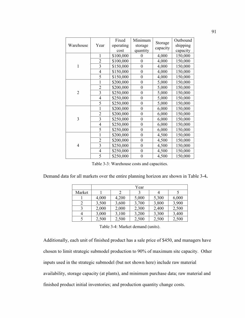
91

Demand data for all markets over the entire planning horizon are shown in Table 3-4.

Additionally, each unit of finished product has a sale price of $450, and managers have

chosen to limit strategic submodel production to 90% of maximum site capacity. Other

inputs used in the strategic submodel (but not shown here) include raw material

availability, storage capacity (at plants), and minimum purchase data; raw material and

finished product initial inventories; and production quantity change costs.

Warehouse Year Fixed

operating cost

Minimum storage quantity

Storage capacity

Outbound shipping capacity

1 $100,000 0 4,000 150,000

2 $100,000 0 4,000 150,000

3 $150,000 0 4,000 150,000

4 $150,000 0 4,000 150,000

1

5 $150,000 0 4,000 150,000

1 $200,000 0 5,000 150,000

2 $200,000 0 5,000 150,000

3 $250,000 0 5,000 150,000

4 $250,000 0 5,000 150,000

2

5 $250,000 0 5,000 150,000

1 $200,000 0 6,000 150,000

2 $200,000 0 6,000 150,000

3 $250,000 0 6,000 150,000

4 $250,000 0 6,000 150,000

3

5 $250,000 0 6,000 150,000

1 $200,000 0 4,500 150,000

2 $200,000 0 4,500 150,000

3 $250,000 0 4,500 150,000

4 $250,000 0 4,500 150,000

4

5 $250,000 0 4,500 150,000

Table 3-3: Warehouse costs and capacities.

Year

Market 1 2 3 4 5

1 4,000 4,200 5,000 5,300 6,000

2 3,500 3,600 3,700 3,800 3,900

3 2,000 2,000 2,300 2,400 2,500

4 3,000 3,100 3,200 3,300 3,400

5 2,500 2,500 2,500 2,500 2,500

Table 3-4: Market demand (units).

92

Data used here as input to the tactical submodel is generally proportional to that

used in the strategic submodel. For example, while input to the strategic submodel

reflects demand at market 1 as 4,000 units in year 1, demand at market 1 in the tactical

submodel is 1,000 units in each of quarters 1 through 4. Furthermore, while not shown

here, transportation times for raw materials and finished products between different

elements in the supply chain range from 1 to 5 days.

Finally, in an effort to explicitly demonstrate the results of changing the priority

order of the three objectives, a disruption in one of the transportation routes is simulated

in the tactical submodel. Specifically, the cost of delivering finished products to market 1

is made prohibitively expensive. The effects of this disruption are discussed when the

numerical results from the example are presented.

3.5.2 Preemptive goal programming solution technique

Before solving the tactical submodel using inputs from the solution to the

strategic submodel, an issue concerning solving preemptive goal programming problems

should be considered. Typically, the solution technique for a preemptive goal

programming problem considers each goal separately, first minimizing deviations from

the most important goal, then the second most important goal, and so on. Of course, all

of these minimizations are first subject to the regular or hard constraints. In each

successive step, the objective function consists only of the deviational variables from the

corresponding goal constraint. Once the first problem is solved, the values of the

deviational variables corresponding to the most important goal constraint are fixed by

93

adding the appropriate constraints to the problem. (Alternatively, the values of the solved

deviational variables may be considered as constants, as is done in the current example.)

This procedure is repeated until all goal constraints have been considered. While the

technique just described is used to solve the numerical example presented here, it is

important to note that more efficient algorithms for preemptive goal programming

problems have been developed. One such method, the partitioning algorithm for (linear)

goal programming (PAGP), thoroughly described by Arthur and Ravindran (1980), has

been shown to be capable of cutting computation time by more than 75% when compared

to other techniques for solving preemptive goal programming problems. Depending on

problem size, such an algorithm may provide a significant advantage when implementing

the two-phase model developed here.

3.5.3 Results

This numerical example was formulated and solved using Extended LINGO 9.0

optimization software. The sizes of the strategic and tactical submodel formulations are

shown in Table 3-5. (These model sizes refer to the case when the profit goal takes top

priority, followed by the demand goal, and then the response time goal.) Notice that the

Variables

Submodel Integer Continuous Total Constraints

Strategic 70 435 505 457

Tactical (run 1) 300 2564 2864 1986

Tactical (run 2) 300 2563 2863 1986

Tactical (run 3) 300 2463 2763 1986

Table 3-5: Numerical example model size (profit first).

94

number of tactical submodel decision variables decreases with each successive

optimization, since deviational variables for the profit and demand goals are fixed as

constants after the first and second optimization runs, respectively. The solution to the

strategic submodel (which took nearly zero processing time) provides an optimal profit

target of $5,643,366, along with the supply chain infrastructure plan, which includes

supplier selections for critical raw materials (see Table 3-6.) In this solution, plants are to

be constructed at locations 1, 2, and 3 in year 1. (In the tactical submodel, this

corresponds to constructing plants at locations 1, 2, and 3 in quarter 1.) Furthermore, the

operating schedule for all four warehouses is summarized in Table 3-7, while optimal

production quantities for plants 1, 2, and 3 are presented in Table 3-8.

Critical raw material #1 Critical raw material #2

Year

Supplier 1 2 3 4 5 1 2 3 4 5

#1

#2

Table 3-6: Critical raw material supplier selections.

Warehouse

Year 1 2 3 4

1

2

3

4

5

Table 3-7: Warehouse operating schedule.

95

Based upon the optimal production quantities for each of the operating plants over

the five-year planning horizon, and a user-defined production capacity factor of 0.9,u =

production capacities for input to the tactical submodel are shown in Table 3-9.

Using the infrastructure and supplier selection decisions made in the solution to

the strategic submodel, along with higher resolution data (omitted here for brevity), the

tactical submodel was solved to determine non-critical raw material supplier selections

and optimal purchasing, production, inventory, and shipment quantity decisions. Using

Extended LINGO 9.0, each of the three sequential optimizations of the tactical submodel

required three or fewer seconds of processing time. When the profit goal has top priority,

followed by the demand goal, and then the response time goal, an optimal profit level of

$3,131,097 is achieved. Table 3-10 summarizes the optimal production quantities

Plant

Year 1 2 3

1 4950 5400 3600

2 4950 5400 3600

3 4950 5400 3600

4 4950 5400 3600

5 4950 5400 3600

Table 3-8: Strategic submodel optimal production quantities.

Plant Plant

Quarter 1 2 3 Quarter 1 2 3

1 1,362 1,485 990 11 1,362 1,485 990

2 1,362 1,485 990 12 1,362 1,485 990

3 1,362 1,485 990 13 1,362 1,485 990

4 1,362 1,485 990 14 1,362 1,485 990

5 1,362 1,485 990 15 1,362 1,485 990

6 1,362 1,485 990 16 1,362 1,485 990

7 1,362 1,485 990 17 1,362 1,485 990

8 1,362 1,485 990 18 1,362 1,485 990

9 1,362 1,485 990 19 1,362 1,485 990

10 1,362 1,485 990 20 1,362 1,485 990

Table 3-9: Tactical submodel production capacities (units).

96

resulting from this implementation of the tactical submodel. Due to the disruption in the

transportation routes leading to market 1 (and the associated prohibitively high shipping

costs), none of the demand for market 1 was met in an effort to maximize overall profits.

However, this situation frees up the necessary resources to satisfy all other demand over

the 5-year planning horizon.

When meeting demand is given the highest priority, followed by meeting or

exceeding the profit goal, and then minimizing response time, the solution indicates a

profit of $1,353,256 over the 5-year planning horizon. This lower profit figure can be

attributed to the tactical submodel attempting to first minimize unsatisfied demand,

despite the prohibitively high costs associated with the disrupted transportation routes to

market 1. Indeed, this case resulted in only 6,145 units of unsatisfied demand, compared

to the 24,500 units of unsatisfied demand in the profit-first case. Figure 3-3 compares the

profit goal achievement levels for the profit-first and demand-first cases. While both

profit goal achievement levels fall well short of the original profit goal due to the

prohibitively high shipping costs corresponding to transportation routes leading to market

Plant Plant

Quarter 1 2 3 Quarter 1 2 3

1 1,362 1,009 250 11 1,362 1,388 250

2 1,362 1,246 250 12 1,362 1,388 250

3 1,362 1,485 250 13 1,362 1,313 250

4 1,362 1,485 250 14 1,362 1,238 250

5 1,362 1,485 250 15 1,362 1,238 250

6 1,362 1,485 250 16 1,362 1,189 250

7 1,362 1,485 250 17 1,362 1,189 250

8 1,362 1,485 250 18 1,362 1,040 250

9 1,362 1,241 250 19 1,362 1,040 250

10 1,362 1,288 250 20 1,362 1,040 250

Table 3-10: Tactical submodel optimal production (profit first).

97

1, this example is meant to demonstrate the ability to conduct tradeoff analysis using the

deterministic tactical submodel.

Table 3-11 summarizes the optimal production quantities resulting from this

implementation of the tactical submodel, while Table 3-12 shows the quarterly change in

production at each plant as the demand goal replaces the profit goal as the top priority.

Profit Goal Achievement

$1,353,256

$3,131,097

$5,643,366

$0

$1,000,000

$2,000,000

$3,000,000

$4,000,000

$5,000,000

$6,000,000

100%

55.5%

24%

Goal Profit first Demand first

Figure 3-3: Profit goal achievement as a percentage of goal target.

Plant Plant

Quarter 1 2 3 Quarter 1 2 3

1 1,362 1,485 990 11 1,362 1,485 990

2 1,362 1,485 990 12 1,362 1,485 990

3 1,362 1,485 990 13 1,362 1,485 975

4 1,362 1,485 990 14 1,362 1,485 868

5 1,362 1,485 990 15 1,362 1,485 863

6 1,362 1,485 990 16 1,362 1,485 863

7 1,362 1,485 990 17 1,362 1,485 990

8 1,362 1,485 990 18 1,362 1,485 990

9 1,362 1,485 990 19 1,362 1,485 990

10 1,362 1,485 990 20 1,362 1,485 990

Table 3-11: Tactical submodel optimal production (demand first).

98

Clearly, plant 3, which operates at its minimum production rate when profit achievement

takes top priority, provides most of the additional production necessary to fulfill demand

when the minimization of unsatisfied demand is set as the #1 goal.

Table 3-13 presents the distribution of unsatisfied demand over all markets and periods in

both the profit-first and demand-first cases. As expected, the achievement level for the

demand satisfaction goal increases when it is assigned top priority (see Figure 3-4).

However, since demand alone is not affected by the prohibitively high shipping costs

assigned to all shipping routes leading to market 1, the change in the achievement level as

the demand satisfaction goal moves from 1st to 2nd or 2nd to 1st priority is not as drastic as

that of the profit goal.

Plant Plant

Quarter 1 2 3 Quarter 1 2 3

1 0 +476 +740 11 0 +97 +740

2 0 +239 +740 12 0 +97 +740

3 0 0 +740 13 0 +172 +725

4 0 0 +740 14 0 +247 +618

5 0 0 +740 15 0 +247 +613

6 0 0 +740 16 0 +296 +613

7 0 0 +740 17 0 +296 +740

8 0 0 +740 18 0 +445 +740

9 0 +244 +740 19 0 +445 +740

10 0 +197 +740 20 0 +445 +740

Table 3-12: Production change as demand goal replaces profit goal as top priority.

99

Market

1 2 3 4 5

Qtr Profit Demand Profit Demand Profit Demand Profit Demand Profit Demand

1 1,000 0 0 0 0 0 0 0 0 0

2 1,000 0 0 0 0 0 0 0 0 0

3 1,000 0 0 0 0 0 0 0 0 0

4 1,000 0 0 0 0 0 0 0 0 0

5 1,050 0 0 0 0 0 0 0 0 0

6 1,050 0 0 0 0 0 0 0 0 0

7 1,050 0 0 0 0 0 0 0 0 0

8 1,050 0 0 0 0 0 0 0 0 0

9 1,250 0 0 0 0 0 0 0 0 0

10 1,250 0 0 0 0 0 0 0 0 0

11 1,250 0 0 0 0 0 0 0 0 0

12 1,250 369 0 0 0 0 0 0 0 0

13 1,325 354 0 0 0 0 0 0 0 0

14 1,325 461 0 0 0 0 0 0 0 0

15 1,325 565 0 0 0 0 0 0 0 0

16 1,325 965 0 0 0 0 0 0 0 0

17 1,500 664 0 0 0 0 0 0 0 0

18 1,500 664 0 0 0 0 0 0 0 0

19 1,500 664 0 0 0 0 0 0 0 0

20 1,500 1444 0 0 0 0 0 0 0 0

Total 24,500 6,150 0 0 0 0 0 0 0 0

Profit first = 24,500 units Overall shortage Demand first = 6,150 units

Table 3-13: Demand shortages (profit first/demand first.)

Demand Goal Achievement

76,550

58,200

82,700

0

10,000

20,000

30,000

40,000

50,000

60,000

70,000

80,000

90,000

Units

100%

70.4%

92.6%

Goal Profit first Demand first

Figure 3-4: Demand goal achievement as a percentage of goal target.

100

3.6 Deterministic model summary

The two-phase model formulated in this chapter provides a tool for supply chain

designers and operators to optimize the supplier selection, purchasing, production,

shipping, and inventory decisions for a single product manufacturing and distribution

network. The strategic submodel first gives supply chain designers an opportunity to

establish the initial supply chain infrastructure for the overall manufacturing and

distribution network that will maximize overall profit. With detailed information

pertaining to non-critical raw material costs and availability, transportation times, and

customer demand, supply chain operators can use this newly obtained information, along

with the results of the strategic submodel, as input to the tactical submodel to determine

optimal non-critical raw material supplier selections and (revised) optimal production,

inventory, and shipment quantities. A simple numerical example was presented to

demonstrate the ease of implementation of the integrated, two-phase model, and the

optimization software LINGO was used to solve both the strategic and tactical

submodels.

While the two-phase model developed here provides an effective tool for the

optimization of supply chain design and operation decisions, it fails to take into account

the uncertainty inherent in real world manufacturing and distribution networks. Without

considering variability in such input parameters as costs and demand, supply chain

managers are likely to make decisions that can lead to suboptimal profit and customer

service. The next chapter addresses this limitation of the two-phase model by altering the

decision makers’ objectives and introducing two stochastic optimization techniques—

101

robust optimization and chance-constrained goal programming—into the strategic and

tactical submodels, respectively, allowing both submodels to accommodate uncertain

input data in their formulations.

102

Chapter 4

SCENARIO-BASED, MULTI-OBJECTIVE,

STOCHASTIC STRATEGIC SUBMODEL

4.1 Introduction

The deterministic supply chain model developed in Chapter 3 assumes all costs,

transportation times, raw material availability, and demand information are known with

certainty. As noted by Gupta and Maranas (2003), this is a highly optimistic assumption,

and failing to consider variability and/or uncertainty can seriously degrade a supply

chain’s performance in the real world, where demand fluctuates, prices change,

production capacities vary, and a variety of disruptions and catastrophes, both natural and

manmade, can occur. In this chapter, a modified version of the supply chain scenario

presented in Chapter 3 is assumed, in which long-term demand forecasts are subject to

uncertainty, while the remaining input parameters are known with certainty, as in the

deterministic case. Here, at the onset of the supply chain design phase, it is assumed that

this uncertain data is available via discrete economic scenarios, each with an estimated

probability of occurrence. Such economic scenarios are considered for long-range

planning purposes, where time periods are assumed to be one or more years in length.

Suppose, for instance, that a long-term forecast of demand data (e.g., annual demand in

each market over a 5- or 10-year planning horizon) is developed based upon the

probability of occurrence of each of four future economic states: strong, good, fair, and

weak. In other words, a demand forecast is made available for each of these four possible

103

economic scenarios, each having an estimated probability of occurrence. Since product

demand depends upon a multitude of factors requiring input from several sources, such a

long-term forecast might be developed using a technique such as the Delphi method.

[This technique, developed by the RAND Corporation, involves gaining a consensus

solution from a panel of experts who remain anonymous relative to one another. See

Dalkey (1969) for an in-depth description of the Delphi method.] The submodel in this

chapter considers the case where decision makers have indicated their desire for a supply

chain design plan that provides the highest possible profit under any possible economic

scenario, with a controllable measure of profit (or cost) variability, while at the same time

minimizing unsatisfied demand. (Recall that the deterministic strategic submodel in

Chapter 3 merely limited market deliveries to forecasted demand and did not specifically

seek to minimize unsatisfied demand.)

The modified design phase scenario, in which demand forecast data is known via

discrete economic scenarios, presents a more realistic problem to managers who must

make supply chain design decisions using imperfect or uncertain data. As Leung and Wu

(2004) imply, however, it is likely that some conditions will prohibit both optimal profits

and 100% customer service levels (in terms of meeting demand) under all possible

economic scenarios. In order to address this problem of future uncertainty, Leung and

Wu (2004), Leung, et al. (2007), and others have applied robust optimization to measure

the tradeoff between solution robustness (i.e., achieving a profit that is close to optimal

for every possible scenario) and model robustness (i.e., developing a solution that almost

meets customer demand under every possible scenario). This approach will be applied to

the strategic submodel developed in Chapter 3 to counter the risk that is inherent in real-

104

world supply chain design and operation problems. Once the stochastic version of the

strategic submodel is completed, its outputs, including critical raw material supplier

selections and optimal supply chain infrastructure decisions, will be used as inputs to a

revised stochastic tactical submodel.

4.2 Stochastic optimization review

In order to establish the necessary background for the revised submodels

developed here and in the next chapter, this section provides a brief review of stochastic

optimization concepts. The two distinct methodologies used to represent uncertainty in

stochastic programming techniques are the scenario-based and distribution-based

approaches (Gupta and Maranas, 2003). In the scenario-based approach, a set of discrete

future scenarios is generated, where each scenario describes a discrete value for some

uncertain parameter(s) and is associated with a probability of occurrence determined by a

decision maker. Examples of scenario-based approaches to stochastic supply chain

problems include the works of Guillén, et al. (2005), Leung, et al. (2006), Santoso, et al.

(2005), and Alonso-Ayuso, et al. (2003). As noted by Gupta and Maranas (2003),

however, the requirement to forecast all possible outcomes of an uncertain parameter

limits the applicability of this approach. When generating a discrete set of scenarios for

uncertain parameters is difficult or impossible, the distribution-based approach may be

used. In this case, a probability distribution is assigned to the continuous range of

potential outcomes for the uncertain parameter(s).

105

According to Sen and Higle (1999), the two solution approaches most widely

studied in the stochastic programming literature are the recourse and chance-constrained

methods. In two-stage recourse models, decision variables are classified by the timing of

their implementation: before (first-stage) or after (second-stage) the values of random

variables are realized. The second-stage or control variables represent “wait and see”

reactive decisions that are contingent on both the first-stage, “here and now” proactive

decisions and the realizations of the uncertain parameters. The recourse (second-stage)

decisions reflect the decision maker’s adaptation to the unfolding of uncertain

events/scenarios. In a production-planning model, for example, manufacturing decisions

may be made before demand quantities are known with certainty. Once the uncertainty

of customer requirements is realized, logistics decisions are made in a way so as to best

satisfy demand [Gupta and Maranas (2003)]. Furthermore, as Sen and Higle (1999) note,

penalty costs may be applied in a recourse model to account for possible infeasibilities

due to the inherent uncertainty. However, when some measure of infeasibility is deemed

to be acceptable, such as a specific loss-of-load probability in power generation planning,

probabilistic constraints (i.e., chance-constrained programming) might be applied (Sen

and Higle, 1999).

In chance-constrained programming, pioneered by Charnes and Cooper (1959),

probabilistic constraints take on two defining characteristics:

1) either the technological coefficients or right hand side values (or both) are not

known with certainty, and

2) the constraint is to be achieved with a certain probability or confidence level.

106

Such a construct allows for a pre-determined measure of infeasibility, as mentioned

above. As a simple example, if a chance constraint is to be met with 95% probability,

this allows for a 5% chance of infeasibility without the penalty that may have been

incorporated into a corresponding recourse model formulation. (A more in-depth review

of chance-constrained programming is presented in Chapter 5.)

While only a brief introduction to the terms and concepts of stochastic

programming is presented, this section serves as a stepping stone to a more in-depth

review of robust optimization in the next section.

4.3 Robust optimization review

The overview of robust optimization presented in this section, which is based on

the descriptions given by Mulvey, et al. (1995) and Leung, et al. (2007), provides the

necessary foundation for adapting the deterministic strategic submodel to the case where

certain inputs are known via discrete economic scenarios. For a more in-depth discussion

of robust optimization with applications, see Greenberg and Morrison (2008).

As discussed in Chapter 2, Mulvey, et al. (1995) developed a scenario-based

robust optimization model that integrates goal programming techniques and incorporates

the conflicting objectives of solution robustness (i.e., always being “close” to optimal)

and model robustness (i.e., always being “almost” feasible). In building the general

framework for the robust optimization model, Mulvey, et al. (1995) first describe the

notions of structural and control variables in a stochastic optimization model. Structural

or design (i.e., first stage) variables are those whose optimal values are not dependent

107

upon the realization of uncertain input parameters. Furthermore, the design variables’

values cannot be adjusted once a realization of the uncertain data is known. On the other

hand, the optimal values of control (i.e., second stage) variables depend upon the

realization of uncertain parameters, as well as the optimal values of the design variables.

The basic stochastic optimization model using design and control variables is presented

as

In this model, Ax b= represents the structural or design constraints, whose coefficient

and right hand side values are known with certainty. On the other hand, Bx Cy e+ =

represents the control constraints, whose coefficients and/or right hand side values are

subject to uncertainty. (Note: The notation in this section should not be confused with

that used in the previous chapter. Once the general discussion of robust optimization is

complete, specific notation similar to that used in the previous chapter will again be

adopted.) Next, a set of scenarios 1, 2,3,..., SΩ = is introduced, where each scenario

s∈Ω has a probability of occurrence ps, with 1

1.S

s

s

p=

=∑ Since each scenario is used to

reflect different values for the (uncertain) input data, a set of control variables (vectors)

1 2 3 , , ,..., ,Sy y y y one for each scenario, is introduced. Now, the robust optimization

model is formulated as

Minimize

subject to ;

;

, 0.

T Tc x d y

Ax b

Bx Cy e

x y

ξ = +

=

+ =

≥

(4.1)

108

where the set 1 2 , ,..., Sz z z contains the error vectors that measure the permitted

infeasibility in the control constraints s s s sB x C y e+ = under scenario s, and the

realizations of the coefficients of the control constraints for each scenario s comprise the

set , , , .s s s sd B C e Furthermore, the previous objective function T Tc x d yξ = + becomes

a random variable of value T T

s s sc x d yξ = + with probability ps. The next step is to

choose an appropriate function for 1( , ,..., )Sx y yσ . In stochastic linear programming, the

function typically used is

which represents the mean or expected value of T T

s s sc x d yξ = + over all scenarios. The

second term in the objective function of formulation 4.2 represents an infeasibility

penalty function. Using the values of the realized error vectors, this function penalizes

violations of the control constraints under some of the scenarios. In other words, this

term allows the model to handle scenarios in which realizations of the uncertain

parameters would otherwise not allow for a feasible solution, albeit with an associated

penalty for each violation of a control constraint. Hence, the first term in the objective

function provides a measure of solution robustness—remaining “close” to optimal for

any realization of the scenario s∈Ω , whereas the second term provides a measure of

model robustness—remaining “close” to feasible for any realization of s∈Ω .

1 1Minimize ( , ,..., ) ( ,..., )

subject to ;

, ;

0, 0, ,

S S

s s s s

s

x y y z z

Ax b

B x C y e s

x y s

σ ωρ+

=

+ = ∀ ∈Ω

≥ ≥ ∀ ∈Ω

(4.2)

1( , ,..., ) , ,S s s

s

x y y p sσ ξ∈Ω

= ∈Ω∑ (4.3)

109

Furthermore, the parameter ω is used as a weight to define the desired tradeoff between

solution and model robustness. As Leung, et al. (2007) point out, assigning a value of

zero to ω may result in an infeasible solution, whereas assigning a sufficiently large value

to ω causes the infeasibility penalty function term to dominate the objective function,

thereby resulting in a higher expected value for 1( , ,..., ).Sx y yσ .

In a supply chain design and operation scenario, a high level of risk may be

associated with one or more of the uncertain input parameters (e.g., raw material

availability or market demand). However, when Eq. 4.3 is used as a cost term in the

objective function of formulation 4.2, the model seeks only to minimize the expected

value of the overall cost across all possible scenarios. In other words, the model does not

account for the potential variability in cost (across scenarios) associated with the high

risk parameter(s). Given this situation, Mulvey, et al. (1995) propose a mean/variance

approach as one technique for mitigating the risk associated with one or more uncertain

input parameters. Specifically, the revised cost function consists of the expected value of

the random variable T T

s s sc x d yξ = + plus a constant times the variance. In other words,

the cost function portion of the objective function in formulation 4.2 becomes

Clearly, as the value of λ is increased, the solution becomes less sensitive to changes in

the data as defined by the scenarios. Mulvey, et al. (1995) point out that this inclusion of

the weighted variance term (i.e., considering a higher moment of T T

s s sc x d yξ = + )

enables robust optimization to account for a decision maker’s preferences toward risk.

2

1( , ,..., ) ( ) ( ) .S s s s s s s

s s s

x y y p p pσ σ ξ λ ξ ξ′ ′′∈Ω ∈Ω ∈Ω

= ⋅ = + −∑ ∑ ∑ (4.4)

110

Thus, robust optimization allows for a more passive management style, giving it a

distinct advantage over stochastic linear programming. In other words, with variability

under control, minimal adjustment to the control variables will be required when the

weighted variance version of robust optimization is applied.

While Eq. 4.4 accounts for both expected cost and cost variability, its quadratic

terms introduce the undesirable characteristic of nonlinearity into the model. As Leung,

et al. (2007) point out, Yu and Li (2000) propose an alternate formulation for Eq. 4.4 as

However, despite eliminating the quadratic terms of Eq. 4.4, the formulation remains

nonlinear. While a direct linearization of the absolute value term in Eq. 4.5 is possible,

the result is the introduction of several constraints and non-negative deviational variables

into the model. Observing this, Yu and Li (2000) propose a more efficient linearization

technique that adds fewer constraints and variables. This technique, as adapted by

Leung, et al. (2007), transforms the minimization of Eq. 4.5 into

Using the framework developed by Yu and Li (2000), Leung, et al. (2007) show that the

minimization of Eq. 4.5 is equivalent to formulation 4.6 as follows. If 0,s s s

s

pξ ξ∈Ω

− ≥∑

then 0sΘ = in the optimal solution. Hence, ( ) .s s s s s s

s s s

p p pσ ξ λ ξ ξ′ ′′∈Ω ∈Ω ∈Ω

⋅ = + −

∑ ∑ ∑

( ) .s s s s s s

s s s

p p pσ ξ λ ξ ξ′ ′′∈Ω ∈Ω ∈Ω

⋅ = + −∑ ∑ ∑ (4.5)

Minimize ( ) 2

subject to 0;

0.

s s s s s s s

s s s

s s s s

s

s

p p p

p

σ ξ λ ξ ξ

ξ ξ

′ ′′∈Ω ∈Ω ∈Ω

∈Ω

⋅ = + − + Θ

− +Θ ≥

Θ ≥

∑ ∑ ∑

∑ (4.6)

111

Otherwise, if 0,s s s

s

pξ ξ∈Ω

− <∑ then s s s s

s

p ξ ξ∈Ω

Θ = −∑ in the optimal solution, and

( ) .s s s s s s

s s s

p p pσ ξ λ ξ ξ′ ′′∈Ω ∈Ω ∈Ω

⋅ = + −

∑ ∑ ∑ Thus, the cost term to be used in formulation

4.2 is transformed from a quadratic form to a much more tractable linear form. Finally,

the resulting linear robust optimization formulation becomes

where .T T

s s sc x d yξ = + The remainder of this chapter shows how the strategic submodel

developed in the previous chapter can be adapted to this robust optimization formulation.

4.4 Notation

As mentioned earlier, it is assumed that managers have provided the following

objectives in the design phase of the supply chain problem (when demand forecasts are

scenario-based):

(1) maximize (expected) profit,

(2) minimize profit variability, and

(3) minimize unsatisfied demand.

Based on these objectives, the scenario-based demand data and other input parameters,

and the generalized robust optimization formulation described above, the deterministic

1Minimize 2 ( ,..., )

subject to ;

, ;

0;

0, , 0, ,

s s s s s s s S

s s s

s s s s

s s s s

s

s s

p p p z z

Ax b

B x C y e s

p

x y s

ξ λ ξ ξ ωρ

ξ ξ

′ ′′∈Ω ∈Ω ∈Ω

∈Ω

+ − + Θ +

=

+ = ∀ ∈Ω

− +Θ ≥

≥ Θ ≥ ∀ ∈Ω

∑ ∑ ∑

∑ (4.7)

112

strategic submodel developed in Chapter 3 will be transformed into a stochastic model

for use in supply chain design problems under demand uncertainty. However, certain

notation must first be added/modified to reflect the scenario-based nature of the problem.

First, the subscript s is introduced, representing a specific economic scenario in the set

1, 2,3,..., .SΩ = Since this subscript can be easily confused with the notation used in

Chapter 3 for the finished product sales price, the following data variable is used in place

of sFP:

sales price per unit of finished product.FPψ =

Then, since each economic scenario has an estimated probability of occurrence, the

following notation is added:

probability that economic scenario will occur.sp s= ∈Ω

Assuming market demand is forecasted via economic scenarios, the following data

variable replaces the corresponding one used in Chapter 3:

demand for finished product at market in period under scenario .s

ptd p t s=

Furthermore, due to the nature of manufacturing and distribution operations, many of the

decisions to be made via the solution to the strategic submodel must be done prior to the

realization of any specific economic scenario (and hence, the realization of any particular

demand forecast). These decisions include

(1) supply chain infrastructure decisions,

(2) critical raw material supplier selection decisions,

(3) all raw material purchasing and shipment quantity decisions,

(4) production quantity decisions,

113

(5) raw material and finished product (plant) inventory quantity decisions, and

(6) plant-to-warehouse shipment quantity decisions.

Therefore, the corresponding decision variables are considered design variables (i.e.,

independent of the realization of scenario s) in the stochastic version of the strategic

submodel. However, supply chain managers do not intend to determine warehouse

finished product inventories or warehouse-to-market shipment quantities until actual

demand data becomes available. Therefore, the variables corresponding to these

decisions will be considered control variables (i.e., dependent upon both the realization of

scenario s and the optimal value of the design variables). Hence, the following notation

will be used in place of the corresponding terms from the previous chapter:

dem

amount of finished product held in inventory at warehouse in period under

scenario ;

amount of finished product shipped from warehouse to market in period

under scenario ;

s

nt

s

npt

h n t

s

z n p t

s

d

=

=

- negative deviational variable related to under-fulfillment of demand at market

in period under scenario .

s

pt p

t s

− =

With this modified notation, the following sections describe the adaptation of the

deterministic strategic submodel to the case where demand data is estimated via discrete

economic scenarios. Since this submodel takes on goal programming characteristics, the

constraints are formulated first, followed by the objective function.

114

4.5 Constraints

While the objective function of the modified strategic submodel will seek to

maximize profits while minimizing profit variability and unsatisfied demand, many of the

constraints take on the same form as those developed in the deterministic version of the

strategic submodel. Considered design constraints, these include Eqs. 3.9, 3.10, 3.12,

3.16 through 3.28, and 3.30. (The use of the term design here corresponds to constraints

containing “first stage” decision variables; such constraints are not necessarily strictly

associated with the design of the supply chain infrastructure.) However, other constraints

must be altered or added to account for the uncertainty in the demand data and the

modified objective function. These control constraints are described as follows.

4.5.1 Warehouse flow conservation (finished products)

The number of units of finished product held in inventory in warehouse n during

period t under scenario s is equal to the number of units of finished product held in

inventory in warehouse n during the previous period under scenario s plus the number of

units of finished product shipped from all plants to warehouse n during period t minus the

number of units of finished product shipped from warehouse n to all markets during

period t under scenario s. That is,

( 1)

1 1

, 1,..., ; 1,..., ; 1,..., .M P

s s s

n t mnt npt nt

m p

h y z h n N t T s S−= =

+ − = = = =∑ ∑ (4.8)

115

It is important to note here that while s

nth (i.e., the inventory at warehouse n in period t

under scenario s) and s

nptz (i.e., the quantity shipped to market p from warehouse n in

period t under scenario s) are considered control variables dependent upon the scenario

realization, mnty (i.e., the quantity of finished product shipped to warehouse n from plant

m in period t) is a design variable independent of the realized scenario. Furthermore, it is

assumed that an initial (known) inventory 0nh of finished product is on hand at each

warehouse at the beginning of the initial period, regardless of the scenario to be realized.

4.5.2 Warehouse capacity and selections

The number of units of finished product held in inventory at warehouse n during

period t under scenario s is limited to a known inventory capacity. Hence,

Furthermore, if warehouse n is open in period t, it must store at least qn units of

finished product in that period. That is,

Additionally, each open warehouse has a defined outbound shipping capacity OUTW

nR .

Hence,

, 1,..., ; 1,..., ; 1,..., .s HFW

nt nt nth C n N t T s Sδ≤ = = = (4.9)

, 1,..., ; 1,..., ; 1,..., .s

nt n nth q n N t T s Sδ≥ = = = (4.10)

1

, 1,..., ; 1,..., ; 1,..., .P

s OUTW

npt n nt

p

z R n N t T s Sδ=

≤ = = =∑ (4.11)

116

4.5.3 Ending inventory requirement

Since supply chain operations are expected to continue beyond the initial planning

horizon considered in the model, a predefined finished product quantity is required to

remain in inventory (i.e., optimally distributed among the plants and/or warehouses)

during the final time period. This carry-over of finished products will ensure initial

inventories are available for follow-on planning. Specifically, the sum of the finished

product inventory remaining in all plants and warehouses during the final period must be

greater than or equal to some fraction of the final period’s total demand. When mTg is

the finished product inventory at plant m in the final period, s

nTh is the finished product

inventory at warehouse n in the final period under scenario s, and FINh is the required

fraction of the final period’s total demand that must be maintained in inventory during the

final period, this constraint is expressed as

where 0 1.FINh≤ ≤

4.5.4 Customer demand non-traditional goal constraint

As in the deterministic tactical submodel, supply chain managers wish to exactly

meet demand in the stochastic version of the strategic submodel. However, they realize

that this may not always be possible, particularly given the uncertain nature of the

1 1 1

, 1,..., ,M N P

s FIN s

mT nT pT

m n p

g h h d s S= = =

+ ≥ =∑ ∑ ∑ (4.12)

117

demand forecasts. Therefore, the corresponding control constraint, in the form of a non-

traditional, one-sided goal constraint, is expressed as

where the negative deviational variable dem-

s

ptd − represents the under-achievement of

customer demand at market p in period t under scenario s. Notice that, as in the

deterministic tactical submodel, positive deviations (i.e., excess deliveries to customer

markets) are not permitted. In an attempt to exactly meet the demand of market p in

period t under scenario s (represented by s

ptd ), dem-

s

ptd − is minimized in the objective

function.

4.6 Objective function formulation

As described earlier, it is assumed that managers have established the following

three objectives in the modified supply chain scenario:

(1) maximize overall profits,

(2) minimize profit (cost) variability, and

(3) minimize unsatisfied demand (i.e., exactly meet demand.)

The following subsections detail the formulation of the objective function through the

sequential development of the expected total profit term (objective 1), the profit

variability term (objective 2), and the infeasibility penalty term (objective 3).

dem-

1

, 1,..., ; 1,..., ; 1,..., ,N

s s s

npt pt pt

n

z d d p P t T s S−

=

+ = = = =∑ (4.13)

118

4.6.1 Profit terms

As in both deterministic submodels presented in Chapter 3, profit in the stochastic

strategic submodel is defined as total supply chain revenue (TR) minus total supply chain

cost (TC). Here, this is expressed as

where the superscript S-STR indicates that the corresponding term is associated with the

stochastic strategic submodel, and the subscript s corresponds to a specific scenario

realization. In the current submodel, total supply chain revenue is calculated by

multiplying the finished product unit sales price by the total number of finished product

units sent to all markets over the entire planning horizon under scenario s. In other

words,

(Recall that the notation for the finished product sales price has been changed in the

current submodel to avoid confusion with the notation for the economic scenarios.) As

before, the costs associated with the supply chain include plant construction costs (CNS-

STR); plant and warehouse fixed operating costs (FCS-STR); raw material costs (RM

S-STR);

variable production costs (PCS-STR); production quantity change costs (PQ

S-STR); shipping

costs (SCS-STR); and holding costs (HC

S-STR). The total cost (TCS-STR) for a given planning

horizon can then be expressed as

Profit – ,S STR S STR S STR

s s sTR TC− − −= (4.14)

1 1 1

, .N P T

S STR FP s

s npt

n p t

TR z sψ−

= = =

= ∈Ω∑∑∑ (4.15)

.

S -STR S -STR S -STR S -STR S -STR

S -STR S -STR S -STR

TC CN FC RM PC

PQ SC HC

= + + +

+ + + (4.16)

119

Of the costs comprising TCS-STR, only the terms for shipping (SC

S-STR) costs and holding

costs (HCS-STR) are directly affected by the introduction of uncertainty into the strategic

submodel. Therefore, these costs are reformulated here, with Eqs. 3.4 through Eq. 3.7

and Eq. 3.11 from the deterministic strategic submodel being used to represent the

remaining unchanged cost terms.

4.6.1.1 Shipping costs for raw materials and finished products

As in Chapter 3, shipping costs (SCS-STR) are calculated for the shipment of critical

and non-critical raw materials from all suppliers to all plants, for the shipment of finished

products from all plants to all warehouses, and for the shipment of finished products from

all warehouses to all markets over the entire planning horizon. Recall, however, that

shipping costs for non-critical raw materials are known only in the aggregate in the

strategic submodel and are not associated with specific suppliers. Furthermore, since

warehouse-to-market shipment quantities now depend upon the realization of scenario s,

the corresponding term in SCS-STR must be slightly modified. Hence, overall shipping

costs are calculated as

1 1 1 1 1 1 1

1 1 1 1 1 1

, .

I K M T I M TS-STR SRP SRP

s ikmt ikmt imt imt

i k m t i I m t

M N T N P TSFW SFM s

mnt mnt npt npt

m n t n p t

SC c w avc w

c y c z s

′ ′

′= = = = = + = =

= = = = = =

= +

+ + ∈Ω

∑∑∑∑ ∑ ∑∑

∑∑∑ ∑∑∑ (4.17)

120

4.6.1.2 Holding costs for raw materials / finished products at plants and warehouses

As with SCS-STR, the term for holding costs (HC

S-STR) must be slightly modified to

reflect the notation associated with scenario s. Hence, holding costs for raw materials

and finished products held in inventory at all production facilities and for finished

products held in inventory at all warehouses are calculated as

Using the previously defined and revised cost terms described above, total cost

can now be expressed as

In turn, total profit is now expressed as

1 1 1 1 1 1 1

.I M T M T N T

S-STR HRP HFP HFW s

s imt imt mt mt nt nt

i m t m t n t

HC c r c g c h= = = = = = =

= + +∑∑∑ ∑∑ ∑∑ (4.18)

1 1 1 1 1 1

1 1 1 1 1 1 1

1 1 1 1

1

( )

M T M T N TS-STR CON P W

s mt mt mt mt nt nt

m t m t n t

I K M T I M TR R

ikt ikmt it imt

i k m t i I m t

T T M TFP PQ PQ

mt mt mt mt mt mt

m t m t

TSRP

ikmt ikmt

m t

TC c f f

c w avc w

c x c e c e

c w

φ β δ= = = = = =

′ ′

′= = = = = + = =

+ + − −

= = = =

= =

= + +

+ −

+ + +

+

∑∑ ∑∑ ∑∑

∑∑∑∑ ∑ ∑∑

∑∑ ∑∑

∑1 1 1 1 1 1

1 1 1 1 1 1

1 1 1 1 1 1 1

I K M I M TSRP

imt imt

i k i I m t

M N T N P TSFW SFM s

mnt mnt npt npt

m n t n p t

I M T M T N THRP HFP HFW s

imt imt mt mt nt nt

i m t m t n t

avc w

c y c z

c r c g c h

′ ′

′= = = + = =

= = = = = =

= = = = = = =

+

+ +

+ + +

∑∑∑ ∑ ∑∑

∑∑∑ ∑∑∑

∑∑∑ ∑∑ ∑∑

(4.19)

121

4.6.1.3 Expected total profit

Since each economic scenario s has an assumed probability of occurrence,

expected total profit can be expressed as

where ProfitS STR

s

− is the random variable defined in Eq. 4.20. Clearly, this term will be

maximized in the objective function.

4.6.1.4 Weighted profit variance term

Following the objective function formulation in Eq. 4.7, the weighted profit

variance term becomes

1 1 1 1 1 1 1 1 1

1 1 1 1 1 1 1

1 1 1

Profit

(

N P T M T M T N TS STR FP s CON P W

s npt mt mt mt mt nt nt

n p t m t m t n t

I K M T I M TR R

ikt ikmt it imt

i k m t i I m t

T T TFP PQ PQ

mt mt mt mt mt mt

m t t

z c f f

c w avc w

c x c e c e

ψ φ β δ−

= = = = = = = = =

′ ′

′= = = = = + = =

+ + − −

= = =

= − − −

− −

− − +

∑∑∑ ∑∑ ∑∑ ∑∑

∑∑∑∑ ∑ ∑∑

∑∑1

1 1 1 1 1 1 1

1 1 1 1 1 1

1 1 1 1 1 1 1

)

.

M

m

I K M T I M TSRP SRP

ikmt ikmt imt imt

i k m t i I m t

M N T N P TSFW SFM s

mnt mnt npt npt

m n t n p t

I M T M T N THRP HFP HFW s

imt imt mt mt nt nt

i m t m t n t

c w avc w

c y c z

c r c g c h

=

′ ′

′= = = = = + = =

= = = = = =

= = = = = = =

− −

− −

− − −

∑∑

∑∑∑∑ ∑ ∑∑

∑∑∑ ∑∑∑

∑∑∑ ∑∑ ∑∑

(4.20)

Expected total profit Profit ,S STR

s s

s

p −

∈Ω

=∑ (4.21)

Weighted profit variance Profit Profit 2 ,S STR S STR

s s s s s

s s

p pλ − −′ ′

′∈Ω ∈Ω

= − + Θ

∑ ∑ (4.22)

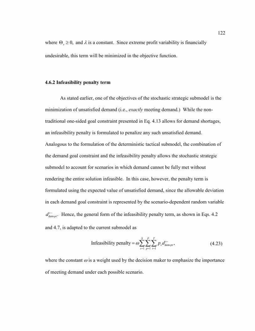
122

where 0,sΘ ≥ and λ is a constant. Since extreme profit variability is financially

undesirable, this term will be minimized in the objective function.

4.6.2 Infeasibility penalty term

As stated earlier, one of the objectives of the stochastic strategic submodel is the

minimization of unsatisfied demand (i.e., exactly meeting demand.) While the non-

traditional one-sided goal constraint presented in Eq. 4.13 allows for demand shortages,

an infeasibility penalty is formulated to penalize any such unsatisfied demand.

Analogous to the formulation of the deterministic tactical submodel, the combination of

the demand goal constraint and the infeasibility penalty allows the stochastic strategic

submodel to account for scenarios in which demand cannot be fully met without

rendering the entire solution infeasible. In this case, however, the penalty term is

formulated using the expected value of unsatisfied demand, since the allowable deviation

in each demand goal constraint is represented by the scenario-dependent random variable

dem- .s

ptd − Hence, the general form of the infeasibility penalty term, as shown in Eqs. 4.2

and 4.7, is adapted to the current submodel as

where the constant ω is a weight used by the decision maker to emphasize the importance

of meeting demand under each possible scenario.

dem-

1 1 1

Infeasibility penalty ,S P T

s

s pt

s p t

p dω −

= = =

= ∑∑∑ (4.23)

123

4.6.3 Overall objective function formulation

By combining the general form of the objective function shown in Eq. 4.6 with

the profit and infeasibility penalty terms formulated in the previous sections, the overall

objective function can be expressed as

Here, the first term reflects the maximization of expected total profit, the second term

reflects the minimization of (weighted) profit variance, and the third term reflects the

minimization of (weighted) expected unsatisfied demand (i.e., infeasibility penalties.)

Furthermore, the use of the λ and ω weights allows decision makers to explore tradeoffs

between solution robustness (i.e., achieving a profit solution that is almost optimal under

every possible scenario) and model robustness (i.e., achieving a solution that almost fully

satisfies demand under every possible scenario), respectively. While Eq. 4.24 is a

complete expression of the multi-criteria objective function for this submodel, two issues

concerning its terms warrant further discussion:

1) the use of criteria weights (i.e., λ and ω), and

2) the use of differing units of evaluation measures (i.e., dollars and units of

finished product.)

First, as mentioned during the development of the deterministic tactical submodel, Masud

and Ravindran (2008) offer several techniques for computing criteria weights in a multi-

criteria decision making problem. These include weights from ranks, the rating method,

dem-

1 1 1

Maximize Profit Profit Profit 2

.

S STR S STR S STR

s s s s s s s

s s s

S P Ts

s pt

s p t

p p p

p d

λ

ω

− − −′ ′

′∈Ω ∈Ω ∈Ω

−

= = =

− − + Θ

−

∑ ∑ ∑

∑∑∑ (4.24)

124

and the ratio weighing method. Next, since the units of evaluation measure differ in

Eq. 4.24, criteria normalization techniques may be applied to allow for an improved

intercriterion comparison. A few of these techniques offered by Masud and Ravindran

(2008) include linear normalization, vector normalization, the use of 10 raised to the

appropriate power, and the use of a range equalization factor.

As before, the appropriate constraints associated with the sΘ variable (see

Eqs. 4.6 and Eq. 4.7) must be included in the overall formulation. These constraints are

expressed as

4.7 Overall formulation

Combining the newly-formed control constraints, the design constraints borrowed

from the deterministic strategic submodel, and the profit/infeasibility penalty objective

function with its associated constraints, the overall robust optimization formulation of the

stochastic strategic submodel becomes

Profit Profit 0, 1,..., ;S STR S STR

s s s s

s

p s S− −′ ′

′∈Ω

− +Θ ≥ =∑ (4.25)

0, 1,..., .s s SΘ ≥ = (4.26)

dem-

1 1 1

Maximize Profit Profit Profit 2

S STR S STR S STR

s s s s s s s

s s s

S P Ts

s pt

s p t

p p p

p d

λ

ω

− − −′ ′

′∈Ω ∈Ω ∈Ω

−

= = =

− − + Θ

−

∑ ∑ ∑

∑∑∑ (4.27)

125

1 1 1 1 1 1 1

1 1 1 1 1 1 1 1 1

subject to

N P T M T M TFP s CON P

npt mt mt mt mt

n p t m t m t

N T I K M T I M TW R R

nt nt ikt ikmt it imt

n t i k m t i I m t

FP

mt

z c f

f c w avc w

c

ψ φ β

δ

= = = = = = =

′ ′

′= = = = = = = + = =

− −

− − −

−

∑∑∑ ∑∑ ∑∑

∑∑ ∑∑∑∑ ∑ ∑∑

1 1 1 1 1 1 1 1

1 1 1 1 1 1 1 1 1

( )

T T M T I K M TPQ PQ SRP

mt mt mt mt mt ikmt ikmt

m t m t i k m t

I M T M N T N P TSRP SFW SFM s

imt imt mnt mnt npt npt

i I m t m n t n p t

x c e c e c w

avc w c y c z

′ ′+ + − −

= = = = = = = =

′= + = = = = = = = =

− + −

− − −

∑∑ ∑∑ ∑∑∑∑

∑ ∑∑ ∑∑∑ ∑∑∑

1 1 1 1 1 1 1

Profit ,

1,... ;

Profit Profit 0, 1,..., ;

I M T M T N THRP HFP HFW s S STR

imt imt mt mt nt nt s

i m t m t n t

S STR S STR

s s s s

s

c r c g c h

s S

p s S

−

= = = = = = =

− −′ ′

′∈Ω

− − − =

=

− +Θ ≥ =

∑∑∑ ∑∑ ∑∑

∑

1

min

1

1

, 1,..., ; 1,..., ; 1,..., ;

, 1,..., ; 1,..., ; 1,..., ;

,

MRS

ikmt ikt ikt

m

M

ikmt ik ikt

m

MRS

imt it

m

w C i I k K t T

w w i I k K t T

w C i I

α

α

=

=

=

′ ′≤ = = =

′ ′≥ = = =

′≤ =

∑

∑

∑

1

1

1,..., ; 1,..., ;

1, 1,..., ;

, 1,..., ; 1,..., ;

, 1,..., ; 1,..., ;

T

mt

t

t

m mt

mt m mt

I t T

m M

m M t T

x uU m M t T

x

ττ

φ

φ β

β

=

=

+ =

≤ =

≥ = =

≤ = =

∑

∑

1

0

, 1,..., ; 1,..., ;

, 1,..., ; 1,..., ;

, 1,..., ; 1,..., ;

0, 1,..., ;

mt m mt

mt mt mt

mt mt mt

m

v m M t T

x x e m M t T

e e e m M t T

x m M

β

−

+ −

≥ = =

− = = =

= − = =

= =

( 1)

1

( 1)

, 1,..., ; 1,..., ;

1,..., ;

, 1,..., ; 1,..., ;

K

im t ikmt i mt imt

k

im t imt i mt imt

r w a x r i I m M

t T

r w a x r i I I m M

′

−=

−

′+ − = = =

=

′+ − = = + =

∑

1,..., ;

, 1,..., ; 1,..., ; 1,..., ;HRP

imt imt mt

t T

r C i I m M t Tβ

=

≤ = = =

126

( 1)

1

, 1,..., ; 1,..., ;

, 1,..., ; 1,..., ;

N

m t mt mnt mt

n

HFP

mt mt mt

g x y g m M t T

g C m M t Tβ

−=

+ − = = =

≤ = =

∑

1

1

( 1)

1 1

, 1,..., ; 1,..., ;

, 1,..., ; 1,..., ;

, 1

NPLANT

mnt m mt

n

MINW

mnt n nt

m

M Ps s s

n t mnt npt nt

m p

y R m M t T

y R n N t T

h y z h n

β

δ

=

=

−= =

≤ = =

≤ = =

+ − = =

∑

∑

∑ ∑ ,..., ; 1,..., ; 1,..., ;

, 1,..., ; 1,..., ; 1,..., ;

, 1,..., ; 1,..., ; 1,..., ;

s HFW

nt nt nt

s

nt n nt

N t T s S

h C n N t T s S

h q n N t T s S

δ

δ

= =

≤ = = =

≥ = = =

1

1 1 1

dem-

1

, 1,..., ; 1,..., ; 1,..., ;

, 1,..., ;

,

Ps OUTW

npt n nt

p

M N Ps FIN s

mT nT pT

m n p

Ns s s

npt pt pt

n

z R n N t T s S

g h h d s S

z d d

δ=

= = =

−

=

≤ = = =

+ ≥ =

+ =

∑

∑ ∑ ∑

∑ 1,..., ; 1,..., ; 1,..., ;

0, 1,..., ; 1,..., ; 1,..., ;

undefined, 1,..., ; 1,..., ; 1,..., ;

imt

imt

p P t T s S

w i I I m M t T

w i I m M t T

= = =

′≥ = + = =

′= = =

0, 1,..., ; 1,..., ; 1,..., ; 1,..., ;

undefined, 1,..., ; 1,..., ; 1,..., ;

1,...

ikmt

ikmt

w i I k K m M t T

w i I k K K m M

t

′ ′≥ = = = =

′ ′= = + =

= , ;

undefined, 1,..., ; 1,..., ; 1,..., ;

1,..., ;

, , , , , , , , ,

ikmt

s s

mt mt mt mnt npt imt mt nt s

T

w i I I k K m M

t T

x e e y z r g h+ −

′= + = =

=

Θ dem- 0, , , , , , ;

, Profit unrestricted, , , ;

binary, 1,..., ; 1,..., ; 1,..., ;

s

pt

S STR

mt s

ikt

d i m n p s t

e m s t

i I k K t Tα

−

−

≥ ∀

∀

′ ′= = =

undefined, 1,..., ; 1,..., ; 1,..., ;

undefined, 1,..., ; 1,..., ; 1,..., ;

, , binary, 1,..., ;

ikt

ikt

mt nt mt

i I k K K t T

i I I k K t T

m M n

α

α

β δ φ

′ ′= = + =

′= + = =

= 1,..., ; 1,..., . N t T= =

This submodel involves (2 2 8 4 ) 2 3T I K IM I I M NS N PS M S′ ′ ′+ + − + + + + + +

constraints and ( 2 7 ) 2T I K M I K IM I M M MN NPS NS N PS S′ ′ ′ ′ ′+ + − + + + + + + +

127

decision variables, of which ( 2 )T I K M N′ ′ + + are integer (binary) variables. Once

again, a change in the number of time periods would have the most impact on the overall

size of the submodel. The numerical example presented in the next section demonstrates

the ability of the stochastic strategic submodel to provide an optimal supply chain

infrastructure solution when long-term demand data is known via discrete economic

scenarios.

4.8 Numerical example

This section provides a numerical example of the stochastic strategic submodel

using the robust optimization formulation described above. The supply chain scenario is

similar to the one provided in Chapter 3 with the following changes. Since this example

only corresponds to the infrastructure design portion of the overall problem, the

objectives are limited to

1) maximizing expected total profit,

2) minimizing profit variability, and

3) minimizing unsatisfied demand (i.e., exactly meeting demand).

Once the stochastic tactical submodel is formulated, these objectives will be altered in the

continuation of the stochastic numerical example.

128

4.8.1 Input data

All appropriate (deterministic) data used in the strategic submodel portion of the

numerical example presented in Chapter 3 is again used here; however, demand data is

replaced by the scenario-based data found in Table 4-1.

(Notice that the demand data associated with the “good” economic scenario correspond to

that used in the deterministic strategic submodel numerical example.) Furthermore, the

probabilities of occurrence associated with the economic scenarios (i.e., strong, good,

fair, and weak) are 0.25, 0.35, 0.25, and 0.15, respectively. Finally, the weights

associated with the profit variance and infeasibility penalty terms are initially (and

arbitrarily) set to 1λ = and 250,ω = respectively.

Year

Market Scenario 1 2 3 4 5

1 Strong 4,200 4,400 5,200 5,500 6,200

Good 4,000 4,200 5,000 5,300 6,000

Fair 3,600 3,800 4,600 4,900 5,600

Weak 2,700 3,300 3,700 4,000 4,700

2 Strong 3,800 3,900 4,000 4,100 4,200

Good 3,500 3,600 3,700 3,800 3,900

Fair 3,200 3,300 3,400 3,500 3,600

Weak 2,400 2,500 2,600 2,700 2,800

3 Strong 2,400 2,400 2,700 2,800 2,900

Good 2,000 2,000 2,300 2,400 2,500

Fair 1,700 1,700 2,000 2,100 2,200

Weak 800 800 1,100 1,200 1,300

4 Strong 3,300 3,400 3,500 3,600 3,700

Good 3,000 3,100 3,200 3,300 3,400

Fair 2,700 2,800 2,900 3,000 3,100

Weak 1,800 1,900 2,000 2,100 2,200

5 Strong 2,900 2,900 2,900 2,900 2,900

Good 2,500 2,500 2,500 2,500 2,500

Fair 2,300 2,300 2,300 2,300 2,300

Weak 1,400 1,400 1,400 1,400 1,400

Table 4-1: Market demand (units)

129

4.8.2 Results

This numerical example was formulated and solved using Extended LINGO 9.0

optimization software. This implementation of the stochastic strategic submodel includes

783 constraints and 973 decision variables (including 70 binary integer variables) and

required 33 seconds of processing time. The solution provides an expected total profit

target of $3,358,170, an expected unsatisfied demand of 12,498 units over the 5-year

planning horizon, and the supply chain infrastructure plan, which includes supplier

selections for critical raw materials (see Table 4-2.) In this solution, plants are to be

constructed at locations 1, 2, and 3 in year 1.

Furthermore, the operating schedule for all four warehouses is summarized in Table 4-3,

while optimal production quantities for plants 1, 2, and 3 are presented in Table 4-4.

Critical raw material #1 Critical raw material #2

Year

Supplier 1 2 3 4 5 1 2 3 4 5

#1

#2

Table 4-2: Critical raw material supplier selections.

Warehouse

Year 1 2 3 4

1

2

3

4

5

Table 4-3: Warehouse operating schedule.

130

Table 4-5 shows the unsatisfied demand for each market in each year (by scenario).

Figure 4-1 provides a snapshot of total demand satisfaction by scenario and market.

Plant

Year 1 2 3

1 4,950 5,400 3,600

2 4,950 5,400 3,600

3 4,950 5,400 2,200

4 4,950 5,400 3,600

5 4,950 5,400 3,600

Table 4-4: Stochastic strategic submodel optimal production quantities.

Year

Market Scenario 1 2 3 4 5

1 Strong 0 0 0 0 0

Good 0 0 0 0 0

Fair 0 0 0 0 0

Weak 0 0 0 0 0

2 Strong 1,500 1,800 4,000 3,200 2,990 Good 0 900 3,400 1,900 1,230

Fair 0 100 2,100 400 0

Weak 0 0 0 0 0

3 Strong 0 2,400 600 300 0

Good 0 2,000 0 0 0

Fair 0 0 0 0 0

Weak 0 0 0 0 0

4 Strong 0 0 0 0 0

Good 0 0 0 0 0

Fair 0 0 0 0 0

Weak 0 0 0 0 0

5 Strong 0 2,900 2,900 0 0

Good 0 2,500 2,500 0 0

Fair 0 2,300 2,300 0 0

Weak 0 0 0 0 0

Table 4-5: Stochastic strategic submodel demand shortages.

131

While the above solution provides the supply chain infrastructure and optimal

expected profit target for use as inputs to the stochastic tactical submodel to be developed

in the next chapter, the parametric structure of the objective function allows for an

analysis of the potential tradeoff between solution robustness and model robustness. That

is, by altering the weights associated with the profit variance and infeasibility penalty

terms, decision makers can gain insight into the tradeoff between optimizing profits (i.e.,

solution robustness) and exactly meeting demand (i.e., model robustness). Figure 4-2

shows the tradeoff between solution robustness and model robustness as the infeasibility

penalty weight changes. This tradeoff analysis allows the decision maker to select an

optimal design solution based upon acceptable ranges of expected unsatisfied demand

and expected total profit.

0

5,000

10,000

15,000

20,000

25,000

30,000

35,000

40,000

45,000

50,000

1 2 3 4 5 1 2 3 4 5 1 2 3 4 5 1 2 3 4 5

Scenario / Market

Units Unsatisfied

Delivered

Strong Good Fair Weak

Figure 4-1: Total demand satisfaction by scenario and market.

132

4.8.3 Comparison with the deterministic strategic submodel solution

A comparison of these results with those from the numerical example associated

with the deterministic strategic submodel can now be made considering the following:

1) demand data for the “good” economic scenario is based upon the demand data

used in the deterministic strategic submodel, and

2) the “good” economic scenario’s 0.35 probability of occurrence is the highest

among the four possible scenarios in the stochastic strategic submodel.

Based on the probabilistic demand forecasts provided in Table 4-1, the demand shortages

and excess deliveries resulting from the solutions to both the deterministic and stochastic

strategic submodels are shown in Table 4-6. Notably, the deterministically-derived

$0

$500,000

$1,000,000

$1,500,000

$2,000,000

$2,500,000

$3,000,000

$3,500,000

$4,000,000

$4,500,000

0 90 190 290 390 490 590

Weight (omega)

Expected Total Profit

(Solution Robustness)

0

5,000

10,000

15,000

20,000

25,000

Expected Unsatisfied Demand

(Model Robustness)

Expected total profit

Expected unsatisfied demand

Figure 4-2: Tradeoff between expected total profit and expected unsatisfied demand.

133

solution results in an expected total demand shortage of 13,691 units, a 9.5% increase

over the 12,498 units of expected shortage resulting from implementation of the

stochastic solution. While excess deliveries were not permitted in the formulations of

either the deterministic or stochastic strategic submodels, Table 4-6 shows how the

deterministically-derived production and distribution schedules would result in a

significant number of excess deliveries if the “fair” or “weak” economic scenarios were

to materialize. (These results are intuitive, since the deterministic strategic submodel’s

demand forecast is essentially a set of point estimates corresponding to the “good”

economic scenario.) Consequently, assuming excess deliveries generate no revenue, both

the “fair” and “weak” scenarios would have a negative impact on the total profit achieved

using the deterministically-derived solution. Specifically, the expected “lost” revenue of

$2,205,450 caused by the expected 4,901 units of excess delivery results in an expected

total profit of $5,643,366 – $2,205,450 = $3,437,916 when the deterministic solution is

implemented in the presence of probabilistic demand. In other words, when excess

deliveries are assumed to generate zero revenue, the expected profit achieved when the

deterministically-derived production and distribution schedules are implemented in the

presence of probabilistic demand is actually 39% lower than the optimal profit reported

Deterministic Stochastic

Scenario Shortage Excess Shortages Excess

Strong 21,030 0 22,590 0

Good 13,030 0 14,430 0

Fair 11,200 5,670 7,200 0

Weak 7,150 23,220 0 0

Expected total

13,691 4,901 12,498 0

Table 4-6: Shortages/excess deliveries relative to stochastic demand.

134

in the point estimate-based solution to the deterministic strategic submodel. Hence,

compared to the profit figure ($3,437,916) achieved by the deterministic strategic

submodel’s optimal production and distribution schedule when probabilistic demand is

considered, the deterministically-derived profit figure (i.e., the $5,643,366 profit based on

point estimate demand values) may be quite misleading to supply chain decision makers.

Finally, while the $3,437,916 profit figure that results from using the deterministically-

derived production and distribution schedules in the presence of probabilistic demand

exceeds the purely stochastic profit solution of $3,358,170 by $79,746 or 2.4%, it does

not reflect the cost of lost sales resulting from the additional 1,193 units of unsatisfied

demand.

While not an entirely “fair” comparison, this brief analysis of the results of the

deterministic and stochastic versions of the strategic submodel should make clear to

decision makers how representing uncertain input parameters such as demand with

average or point estimate values can lead to potentially misleading results, particularly

when the uncertain parameters have the potential to vary widely. On the other hand,

while stochastically-derived production and distribution schedules may not necessarily

provide a higher expected profit figure than their deterministic counterparts do in the

presence of probabilistic demand, the increased customer service levels in terms of

satisfied demand may be well worth the cost to supply chain decision makers.

135

4.9 Stochastic strategic submodel summary

When demand data is forecast via possible future economic scenarios (with

corresponding probabilities of occurrence), the stochastic submodel described in this

chapter can be applied to supply chain design planning problems where managers wish to

1) maximize expected total supply chain profits,

2) minimize profit variability with regard to possible economic scenarios, and

3) minimize expected total unsatisfied demand.

By varying the weights associated with the profit variance and infeasibility penalty terms,

supply chain managers can use this submodel as a flexible tool for analyzing tradeoffs

between achieving an optimal profit solution (i.e., solution robustness) and minimizing

unsatisfied demand (i.e., model robustness). When data related to costs and capacities,

along with scenario-based demand data, are available, this mixed integer linear robust

optimization program can be solved using a variety of commercially-available solvers.

Once solved, the stochastic strategic submodel provides managers with the following

supply chain infrastructure planning elements:

(1) critical raw material supplier selections,

(2) plant construction decisions,

(3) locations of operating plants and warehouses for each period,

(4) input for production capacity requirements, and

(5) an expected total profit goal.

136

As in the deterministic case, the supply chain infrastructure elements listed above are

then used as inputs to a tactical submodel. However, it is assumed that distribution-based

demand data replaces scenario-based demand data once infrastructure decisions have

been made and the operational phase of the supply chain management problem has begun

to evolve. Hence, the stochastic tactical submodel is designed to accept such

distribution-based demand data as input and allow decision makers to set confidence

levels for the achievement of various objectives. The next chapter describes the

formulation of the stochastic tactical submodel and continues the numerical example

presented in the current chapter.

137

Chapter 5

DISTRIBUTION-BASED, MULTI-OBJECTIVE,

STOCHASTIC TACTICAL SUBMODEL

5.1 Introduction

As in the deterministic case, the operational planning phase of the supply chain

problem under uncertainty begins once infrastructure decisions have been made (and

perhaps implemented) via the solution to the (stochastic) strategic submodel. Analogous

to the deterministic scenario, the stochastic tactical submodel described in this chapter

uses as inputs the supply chain infrastructure decisions made via the solution to the

stochastic strategic submodel, along with newly-acquired, near-term cost, demand, and

transit data, to determine revised optimal purchase, production, inventory, and shipment

quantities for both raw materials and finished products. (Once again, these decisions

override those made via the solution to the strategic counterpart.)

While data available to supply chain managers early in the planning process is

likely to be based upon longer time periods (e.g., one year or greater), raw material

availability, cost data, (newly-acquired) transportation times, and demand information are

assumed to be known with higher resolution once the operational phase begins. In fact, it

is assumed here that demand data, previously forecasted via possible economic scenarios,

is now estimated via continuous probability distributions, since the entire planning

horizon is now broken down into shorter time periods (e.g., quarters), and additional

demand information becomes available as the supply chain matures and evolves. As in

138

the scenario presented in the deterministic case, it is assumed here that decision makers

have developed multiple objectives with regard to profits, meeting customer demand, and

minimizing supply chain response time. However, considering the distribution-based

demand data available in this revised scenario, it is assumed that decision makers have

altered their objectives to reflect the nature of the uncertainty in the demand input data.

Acknowledging the potential for uncertainty in the given data to lead to missed

objectives, it is further assumed that decision makers have presented supply chain

managers with confidence levels at which the demand goals are expected to be met.

Now, the objectives for the stochastic tactical submodel become:

(1) meet customer/market demand with specified levels of confidence,

(2) meet a specified profit goal,

(3) minimize supply chain response time.

For instance, instead of merely seeking to minimize unsatisfied demand in the presence

of uncertain demand data, decision makers might now require that demand be met with at

least a 90% confidence level when demand is forecast via probability distributions. In

fact, two additional (yet manageable) complexities, based on demand forecasts and

decision maker preferences, may be introduced into the problem in a real-world supply

chain scenario:

1) probability distributions corresponding to demand may vary by market and/or

period, and

2) assigned confidence levels may vary by market and/or period.

Considering these objectives and possible input complexities, chance-constrained goal

programming is proposed as an appropriate stochastic optimization technique to be

139

applied to a modified version of the tactical submodel. As in Chapter 3, the tactical

submodel will be designed to receive infrastructure inputs from the strategic submodel,

and its solution will provide non-critical supplier selections and optimal purchasing,

shipping, inventory, and production decisions for use in the operational supply chain

phase. Once the stochastic version of the tactical submodel is formulated, the numerical

example presented in Chapter 4 is continued to demonstrate the applicability of the

overall supply chain model under different forms of data uncertainty.

5.2 Chance-constrained goal programming review

This section, based on the descriptions given by Keown and Taylor (1980) and

Rakes, et al. (1984), provides a brief review of the concepts of chance-constrained goal

programming in preparation for its application to the stochastic version of the tactical

submodel in the sections that follow.

In the case where one or more input parameters in an optimization problem are

available only via probability distributions, it is common to simplify the problem by

assuming a mean value for the parameter based on its given distribution. However, such

an approach overlooks the potentially high variability associated with uncertain input

parameters. Furthermore, while post optimality sensitivity analysis can be used to assess

the effects of changing (i.e., uncertain) input parameter values when deterministic linear

programming or goal programming techniques are applied, such analysis may become

extremely difficult when the assessment of simultaneous changes in multiple parameters

is attempted (Rakes, et al., 1984). As a remedy to this problem, chance-constrained

140

programming (CCP) techniques approach such distribution-based uncertainty by

optimizing decision variables when certain goals or constraints are desired to be achieved

with specified probabilities or confidence levels. In other words, CCP allows decision

makers to express a permissible probability of a goal or constraint violation. For

instance, if a decision maker states that a goal should be met with α probability, he or she

is implying the acceptance of not satisfying the goal (1 – α) percent of the time (Keown

and Taylor, 1980). When multiple, non-rigid objectives are expressed via goal

constraints, and the values of certain technological coefficients and goal achievement

targets are known via probability distributions, a basic chance-constrained goal

programming model, as described by Rakes, et al. (1984), can be formulated as

where aij is the technological coefficient associated with the jth decision variable within

the ith row, xj is the jth decision variable, bi is the goal or target value corresponding to

the ith goal, and i id d− + are the negative and positive deviational variables, respectively,

associated with goal constraint i, αi is the minimum desired probability of achieving the

specified target in goal constraint i (with 0 < αi < 1), Pk is the priority level associated

with the achievement of goal constraint i, and and k k

i iw w− + are weights associated with

the deviational variables corresponding to goal constraint i. (As in the previous chapter,

0 1

1

Minimize ( )

subject to , 1,..., ;

and/or 0 , 1,..., ;

, , 0, , .

K mk k

k i i i i

k i

n

ij j i i i

j

i i i

j i i

Z P w d w d

a x d d b i m

P d d i m

x d d i j

α

− − + +

= =

− +

=

− +

− +

= +

+ − = =

= ≥ =

≥ ∀

∑∑

∑ (5.1)

141

the notation used to describe this general formulation should not be confused with the

notation assigned to the specific supply chain problem under consideration. Once the

general discussion of chance-constrained goal programming is complete, specific

notation similar to that used in the strategic and tactical submodels of the previous

chapter will again be adopted.) In the general case, aij and bi are assumed to be

independent random variables with respective means E(aij) and E(bi) and respective

variances 2 ( ) ijaσ and 2 ( ). ibσ As noted by Rakes, et al. (1984), the value (1 – αi)

represents the probability that constraint i will not be realized and is likewise a reflection

of a decision maker’s uncertainty with respect to the achievement of goal constraint i.

In the case where aij and bi are assumed to be normally distributed, and goal

constraint i is assumed to be a less-than-or-equal-to constraint in which id + is to be

minimized, Rakes, et al (1984) present the deterministic equivalent of formulation 5.1 as

In the case where id − is to be minimized (i.e., a greater-than-or-equal-to goal constraint is

assumed), the first constraint in formulation 5.2 is modified as follows:

0 1

2

1

1

22 2

1

Minimize ( )

subject to ( ) ( ) ( ) ,

1,..., ; 1,..., ;

( ) , 1,...,

i i

K mk k

k i i i i

k i

n

ij j i i i i i

j

n

ij j i

j

Z P w d w d

E a x y d d E b b

i m j n

a x y i

α αψ ψ σ

σ

− − + +

= =

− +

=

=

= +

+ + − = −

= =

= =

∑∑

∑

∑ ;

, , , 0.j i i i

m

x y d d− + ≥

(5.2)

142

As noted by Rakes, et al. (1984), either version of formulation 5.2 will be nonlinear

whenever any aij is a random variable (i.e., aij has a nonzero variance.) In this case, a

linearization scheme, such as Naslund’s approximation, may be used to convert

formulation 5.2 to a linear form. (See De, et al., 1982 for one such example.) In contrast

to the nonlinear nature of formulation 5.2, however, Keown and Taylor (1980) show that

the resulting deterministic equivalent is linear when only the target values of the goal

constraints are random variables (i.e., the technological constraints are deterministic.)

Since demand is the only uncertain input parameter used in the development of the

stochastic tactical submodel in this chapter, a derivation of the deterministic equivalent

that parallels that of Keown and Tayor (1980) will be presented here.

As will be shown in the following sections, the combination of non-rigid goals

and distribution-based input parameters makes chance-constrained goal programming a

natural approach for the stochastic version of the tactical submodel.

5.3 Notation

Since demand data is the only input in the stochastic tactical submodel that is not

assumed to be known with certainty, minimal changes to the notation of the deterministic

tactical submodel are needed here. In fact, the only new notation needed relates to the

probabilistic nature of customer demand in this submodel:

2

1

( ) ( ) ( ) ,

1,..., ; 1,..., .

i i

n

ij j i i i i i

j

E a x y d d E b b

i m j n

α αψ ψ σ− +

=

− + − = +

= =

∑ (5.3)

143

2

( ) expected value of demand distribution at market in period ;

( ) variance of demand distribution at market in period ;

= desired confidence level at which demand should be met exactly

pt

pt

pt

E d p t

d p tσ

γ

=

=

at market in period ;

realized value of standard normal random variable related

to customer demand chance-constrained goal;

desired confidence level at which ending inventory should meet

pt

p t

γη

ε

=

=

dem-

or exceed a predefined fraction of total demand in the final period;

realized value of standard normal random variable related

to ending inventory requirement chance constraint;

positive deptd

εκ

+

=

=

dem-

viational variable related to over-achievement of demand

goal at market in period ;

negative deviational variable related to under-achievement of demand

goal at market in period ;

pt

p t

d

p t

− =

With this additional notation, the following sections describe the adaptation of the

deterministic tactical submodel to the case where demand data is estimated via

continuous probability distributions with known parameters. Since this submodel is

formulated as a goal program, the constraints are formulated first, followed by the

objective function.

5.4 Goal constraints

As in the deterministic version of the tactical submodel, the formulation of the

stochastic version includes three goal constraints related to the objectives of exactly

meeting customer demand, meeting or exceeding a certain profit level, and minimizing

total weighted transit time. These goals’ formulations are described as follows.

144

5.4.1 Customer demand goal constraint

Recall that in the deterministic version of the tactical submodel, as well as in the

stochastic version of the strategic submodel, constraints corresponding to the

minimization of unsatisfied demand (i.e., exactly meeting demand) were formulated as

one-sided, non-traditional (equality) goal constraints (see Eqs. 3.48 and Eq. 4.13 ). With

the introduction of distribution-based demand data, along with corresponding decision

maker-provided confidence levels for meeting demand, demand constraints in the

stochastic tactical submodel might then be formulated as

where nptz is the quantity of finished product shipped from warehouse n to market p in

period t, ptγ represents the minimum desired confidence level at which demand at market

p in period t should be exactly met, and ptd is a continuous random variable with

expected value ( )ptE d and variance 2 ( ).ptdσ In other words, Eq. 5.4 reflects decision

makers’ desire that deliveries to market p in period t exactly meet demand with a

probability greater than or equal to ptγ . However, Eq. 5.4 is not a valid constraint for

this submodel, since the probability of a continuous random variable (i.e., ptd ) equaling a

fixed value (i.e., 1

N

npt

n

z=∑ ) is zero. Therefore, the constraint is modified as

1

, 1,..., ; 1,..., ,N

npt pt pt

n

P z d p P t Tγ=

= ≥ = =

∑ (5.4)

1

, 1,..., ; 1,..., .N

npt pt pt

n

P z d p P t Tγ=

≥ ≥ = =

∑ (5.5)

145

Clearly, this revised greater-than-or-equal-to chance constraint does not fully correspond

to decision makers’ desire to exactly meet demand; instead, it reflects the desire that

market deliveries meet or exceed market demand with a (minimum) given confidence

level. While excess deliveries were prohibited in previous submodels, the probabilistic

nature of demand in this case may force a relaxation of this restriction. However, a

strategy for pursuing the goal of meeting demand exactly will be discussed once the

deterministic equivalent of Eq. 5.5 is formulated.

The derivation of the deterministic equivalent constraint for Eq. 5.5 is as follows.

First, it is assumed here that ptd is normally distributed for two reasons:

1) normally distributed demand is widely assumed in supply chain literature, since

the normal distribution “captures the essential features of demand uncertainty and

is convenient to use” (Gupta and Maranas, 2003), and

3) a normal distribution simplifies the derivation of the deterministic equivalent

constraint for Eq. 5.5.

It is further assumed that demand distributions across all markets and time periods are

independent of each other. Consequently, the derivation here parallels the one presented

by Keown and Taylor (1980) for chance constraints whose target values are represented

by normally-distributed random variables with known expected values and variances.

When ( )ptE d is subtracted from both sides of the inequality in Eq. 5.5, and both sides are

divided by ( ),ptdσ the chance constraint can be restated as

146

Since ptd is assumed to be normally distributed, then ( )

( )

pt pt

pt

d E d

dσ

− must follow a

standard normal distribution (i.e., a normal distribution with mean zero and standard

deviation one), as can be shown by deriving the moment-generating function of

( )

( )

pt pt

pt

d E d

dσ

− and comparing it with the moment-generating function of a normal random

variable (Wackerly, et al., 2002). It is then possible to find a value ptpt γη η= such that

where ptη represents a realization of the standard normal random variable ( )

,( )

pt pt

pt

d E d

dσ

−

and the integration term represents the area under the standard normal curve to the left of

the value ptγη (see Figure 5-1.)

1

( )( )

, 1,..., ; 1,..., .( ) ( )

N

npt ptpt ptn

pt

pt pt

z E dd E d

P p P t Td d

γσ σ

=

− −

≥ ≥ = =

∑ (5.6)

21

2( ) 1

, 1,..., ; 1,..., ,( ) 2

pt

pt

pt

pt pt

pt

pt

d E dP e p P t T

d

γηη

γη γσ π

−

−∞

− ≥ = = = =

∫ (5.7)

Figure 5-1: Standard normal plot for demand chance constraint.

ptγη

ptγ

147

Clearly, the area defined by the integration term in Eq. 5.7 (and thus the probability

value) will increase when ptγη is replaced by a larger number. Therefore,

if and only if

Rearranging terms in Eq. 5.9 gives

While a deterministic equivalent constraint (Eq. 5.10) has replaced the original chance

constraint (Eq. 5.5), it still does not address decision makers’ desire to exactly meet

demand. By adding deviational variables to Eq. 5.10, however, it can be converted to a

goal constraint as

The inclusion here of positive deviational variables—which reflect excess market

shipments—results from the probabilistic nature of demand in this scenario. By

minimizing both the negative and positive deviational variables in the objective function,

decision makers can reflect their desire to minimize both unsatisfied demand and excess

shipments, respectively. Furthermore, the fact that the target value for the demand goal

1

( )( )

, 1,..., ; 1,..., ,( ) ( )

N

npt ptpt ptn

pt

pt pt

z E dd E d

P p P t Td d

γσ σ

=

− −

≥ ≥ = =

∑ (5.8)

1

( )

, 1,..., ; 1,..., .( ) pt

N

npt pt

n

pt

z E d

p P t Td

γησ

=

−≥ = =

∑

(5.9)

1

( ) ( ), 1,..., ; 1,..., .pt

N

npt pt pt

n

z E d d p P t Tγη σ=

≥ + = =∑ (5.10)

dem- dem-

1

( ) ( ), 1,..., ; 1,..., .pt

N

npt pt pt pt pt

n

z d d E d d p P t Tγη σ− +

=

+ − = + = =∑ (5.11)

148

constraint (Eq. 5.11) exceeds the expected value of the demand distribution implicitly

places a greater degree of importance on the “minimization of unsatisfied demand”

subgoal than on the “minimization of excess shipments” subgoal. In fact, while decision

makers might wish to minimize both unsatisfied demand and excess shipments, it is

assumed here that there is more managerial focus on meeting demand than on the excess

shipments. The issue of excess shipments (represented by the positive deviational

variables), then, can then be further dealt with by making two minor modifications. First,

by assigning weights to both demand-related deviational variables in the objective

function, decision makers can express the relative importance of minimizing unsatisfied

demand and minimizing excess shipments with respect to one another. For example,

assigning a larger weight to the positive deviational variable represents an attempt to

counter the fact that the demand goal target is some quantity greater than the expected

value. Second, a penalty term related to excess market shipments can be added to the

profit goal constraint. For instance, customer markets may agree—perhaps through

contractual arrangements— to accept shipments in excess of the demand goal target;

however, the cost to the supply chain for this arrangement might be such that shipments

in excess of the expected value of demand plus some multiple (e.g., the realized value of

the standard normal random variable) of the standard deviation will not generate revenue.

In other words, the supply chain incurs the cost of producing and shipping each of these

excess units but does not generate the associated revenue. While other penalty constructs

may be developed, the one described here will be incorporated into the current submodel.

Following Keown and Taylor (1980), the optimal quantity of finished product

sent to market p in period t will be a function of the expected value and variance of the

149

demand distribution at market p in period t and the decision makers’ desired level of

customer satisfaction (as defined by the confidence level at which demand should be

exactly met.)

5.4.2 Profit optimization goal constraint

The goal constraint related to the objective of meeting or exceeding the optimal

profit level as determined in the solution to the stochastic strategic submodel is slightly

modified from the one used in the deterministic version of the tactical submodel. In the

current submodel, a penalty term is added to reflect the fact that no revenue is generated

by sending to markets units of finished product that exceed the expected value plus some

multiple of the standard deviation of the demand distribution for a given market in a

given period. Therefore, the profit optimization goal constraint is expressed as

1 1 1 1 1 1 1

' '

1 1 1 1 1 1 1 1

1 1 1 1 1 1

(

N P T P T M TFP FP CON

npt pt mt mt

n p t p t m t

M T N T I K M TP W R

mt mt nt nt ikt ikmt

m t n t i k m t

I K M T T TR FP PQ PQ

ikt ikmt mt mt mt mt mt

i I k m t m t

z d c

f f c w

c w c x c e c

ψ ψ φ

β δ

+

= = = = = = =

= = = = = = = =

+ +

′= + = = = = =

− −

− − −

− − − +

∑∑∑ ∑∑ ∑∑

∑∑ ∑∑ ∑∑∑∑

∑ ∑∑∑ ∑∑1 1

1 1 1 1 1 1 1 1 1 1 1

1 1 1 1 1 1 1 1

)M T

mt

m t

I K M T I K M T M N TSRP SRP SFW

ikmt ikmt ikmt ikmt mnt mnt

i k m t i I k m t m n t

N P T I M T M TSFM HRP HFP HFW

npt npt imt imt mt mt nt nt

n p t i m t m t

e

c w c w c y

c z c r c g c h

− −

= =

′ ′

′= = = = = + = = = = = =

= = = = = = = =

− − −

− − − −

∑∑

∑∑∑∑ ∑ ∑∑∑ ∑∑∑

∑∑∑ ∑∑∑ ∑∑1 1

profit profit ,

N T

n t

d d Y

= =

− ++ − =

∑∑

(5.12)

150

where the term 1 1

P TFP

pt

p t

dψ +

= =∑∑ represents the penalty for market shipments that exceed the

demand goal target value, and profit profit and d d− + represent the under- and over-achievement,

respectively, of the profit goal Y.

5.4.3 Total weighted transit time goal constraint

The goal constraint related to the objective of minimizing total weighted transit

time (i.e., supply chain response time) is identical to the one used in the deterministic

version of the tactical submodel and is restated here for illustrative purposes:

where time time and d d− + represent the under- and over-achievement, respectively, of the total

weighted transit time goal.

5.5 Ending inventory chance constraint

While most of the “regular” constraints in the stochastic and deterministic tactical

submodels overlap, the inclusion of probabilistic demand values in the constraint

corresponding to ending inventory requirements makes a change to this constraint

necessary. Designed to prevent inventory discrepancies at the end of a multi-period

planning horizon and expressed as Eq. 3.65, this constraint requires a predefined finished

1 1 1 1 1 1 1 1

time time

1 1 1 1 1 1

0,

I K M T I K M TTRP TRP

ikm ikmt ikm ikmt

i k m t i I k m t

M N T N P TTFW TFM

mn mnt np npt

m n t n p t

b w b w

b y b z d d

′ ′

′= = = = = + = = =

− +

= = = = = =

+

+ + + − =

∑∑∑∑ ∑ ∑∑∑

∑∑∑ ∑∑∑ (5.13)

151

product quantity to remain in inventory during the final time period. Specifically, the

sum of the finished product inventory remaining in all plants and warehouses during the

final period must be equal to or greater than some fraction of the final period’s total

demand. However, since demand is now forecast in terms of a continuous probability

distribution, Eq. 3.65 is transformed into a chance constraint as

where hFIN is the fraction of final demand required to be kept in inventory and is assigned

a positive value between zero and one, and ε is the assigned confidence level at which the

ending inventory requirement should be met. In other words, the probability that the sum

of all finished product inventories (i.e., plant and warehouse inventories combined) in the

final period is equal to or greater than some fraction of the sum of all demand in the final

period should meet or exceed some assigned value .ε The deterministic equivalent of the

ending inventory chance constraint is derived as follows.

Since ptd is assumed to be independently normally distributed with mean ( )ptE d

and variance 2 ( )ptdσ for each market 1,...,p P= and period 1,..., ,t T= then 1

P

pT

p

d=∑ is

normally distributed with mean 1

( )P

pT

p

E d=∑ and variance 2

1

( ).P

pT

p

dσ=∑ When

1

( )P

pT

p

E d=∑ is

1 1

1 1 1 1

,

M N

mT nTM N P PFIN m n

mT nT pT pTFINm n p p

g h

P g h h d P dh

ε= =

= = = =

+

+ ≥ = ≥ ≥

∑ ∑∑ ∑ ∑ ∑ (5.14)

152

subtracted from both sides of the inequality in Eq. 5.14, and both sides are divided by

2

1

( )P

pT

p

dσ=∑ , the chance constraint can be restated as

Using the same reasoning as in the derivation of the deterministic equivalent for Eq. 5.5,

1 1

2

1

( )

( )

P P

pT pT

p p

P

pT

p

d E d

dσ

= =

=

−∑ ∑

∑ must follow a standard normal distribution. It is then possible to

find a value εκ κ= such that

where κ represents a realization of the standard normal random variable

1 1

2

1

( )

( )

P P

pT pT

p p

P

pT

p

d E d

dσ

= =

=

−∑ ∑

∑, and the integration term represents the area under the standard

normal curve to the left of the value κε (see Figure 5-2.)

1 1 1 1 1

2 2

1 1

( ) ( )

.

( ) ( )

M N P P PFIN

mT nT pT pT pT

m n p p p

P PFIN

pT pT

p p

g h h E d d E d

P

h d d

ε

σ σ

= = = = =

= =

+ − −

≥ ≥

∑ ∑ ∑ ∑ ∑

∑ ∑ (5.15)

211 1 2

2

1

( )1

,2

( )

P P

pT pT

p p

P

pT

p

d E d

P e

d

εκκ

εκ επ

σ

−= =

−∞

=

−

≥ = =

∑ ∑∫

∑ (5.16)

153

Clearly, the area defined by the integration term in Eq. 5.16 (and thus the probability

value) will increase when κε is replaced by a larger number. Therefore,

if and only if

Rearranging terms in Eq. 5.18 gives

Hence, the optimal ending finished product inventory is a function of the expected values

and variances of the demand distributions for all markets in the final period, along with

the decision maker’s level of risk aversion in terms of the confidence level at which the

Figure 5-2: Standard normal plot for ending inventory chance constraint.

1 1 1 1 1

2 2

1 1

( ) ( )

( ) ( )

M N P P PFIN

mT nT pT pT pT

m n p p p

P PFIN

pT pT

p p

g h h E d d E d

P

h d d

ε

σ σ

= = = = =

= =

+ − −

≥ ≥

∑ ∑ ∑ ∑ ∑

∑ ∑ (5.17)

1 1 1

2

1

( )

.

( )

M N PFIN

mT nT pT

m n p

PFIN

pT

p

g h h E d

h d

εκ

σ

= = =

=

+ −

≥∑ ∑ ∑

∑ (5.18)

2

1 1 1 1

( ) ( ) .M N P P

FIN

mT nT pT pT

m n p p

g h h E d dεκ σ= = = =

+ ≥ +

∑ ∑ ∑ ∑ (5.19)

154

ending inventory should meet or exceed a predefined fraction of total demand in the final

period.

5.6 Regular constraints

In addition to the chance constraints and deterministic goal constraints described

above, the stochastic tactical submodel requires several regular constraints that must be

met for the overall solution to remain feasible. However, the vast majority of these

constraints are identical to those used in the deterministic tactical submodel; they are

Eqs. 3.9, 3.10, 3.12 and Eqs. 3.49 through 3.64.

5.7 Objective function and overall formulation

The objective function for the stochastic tactical submodel takes on the same

general form as that for the deterministic version, since the objectives of meeting or

exceeding a profit goal (as determined by the solution to the stochastic strategic

submodel), exactly meeting customer demand, and minimizing response time are nearly

identical to those in the deterministic case. (The variation, of course, involves the

probabilistic nature of the demand goal constraint.) Therefore, the preemptive goal

programming objective function is expressed as

1 profit 2 dem- dem- 3 time

1 1

Minimize ( ) ,P T

pt pt pt pt

p t

Pd P d d P dλ λ− − − + + +

= =

+ + +∑∑ (5.20)

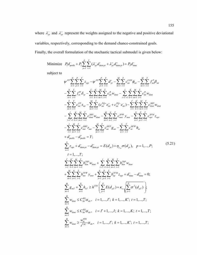
155

where ptλ − and ptλ + represent the weights assigned to the negative and positive deviational

variables, respectively, corresponding to the demand chance-constrained goals.

Finally, the overall formulation of the stochastic tactical submodel is given below:

1 profit 2 dem- dem- 3 time

1 1

1 1 1 1 1 1 1 1 1

Minimize ( )

subject to

P T

pt pt pt pt

p t

N P T P T M T M TFP FP CON P

npt pt mt mt mt mt

n p t p t m t m t

Pd P d d P d

z d c f

λ λ

ψ ψ φ β

− − − + + +

= =

+

= = = = = = = = =

+ + +

− − −

∑∑

∑∑∑ ∑∑ ∑∑ ∑∑' '

1 1 1 1 1 1 1 1 1 1

1 1 1 1 1 1 1

( )

N T I K M T I K M TW R R

nt nt ikt ikmt ikt ikmt

n t i k m t i I k m t

T T M T K M TFP PQ PQ SRP

mt mt mt mt mt mt ikmt ikmt

m t m t k m t

f c w c w

c x c e c e c w

δ′= = = = = = = + = = =

′+ + − −

= = = = = = =

− − −

− − + −

∑∑ ∑∑∑∑ ∑ ∑∑∑

∑∑ ∑∑ ∑∑∑1

1 1 1 1 1 1 1 1 1 1

1 1 1 1 1 1 1

I

i

I K M T M N T N P TSRP SFW SFM

ikmt ikmt mnt mnt npt npt

i I k m t m n t n p t

I M T M T N THRP HFP HFW

imt imt mt mt nt nt

i m t m t n t

c w c y c z

c r c g c h

′

=

′= + = = = = = = = = =

= = = = = = =

− − −

− − −

∑

∑ ∑∑∑ ∑∑∑ ∑∑∑

∑∑∑ ∑∑ ∑∑

profit profit

dem- dem-

1

1

;

( ) ( ), 1,..., ;

1,..., ;

pt

N

npt pt pt pt pt

n

TTRP

ikm ikmt

m t

d d Y

z d d E d d p P

t T

b w

γη σ

− +

− +

=

= =

+ − =

+ − = + =

=

∑

∑1 1 1 1 1 1 1

time time

1 1 1 1 1 1

2

1 1 1

0;

( ) ( )

I K M I K M TTRP

ikm ikmt

i k i I k m t

M N T N P TTFW TFM

mn mnt np npt

m n t n p t

M N PFIN

mT nT pT pT

m n p p

b w

b y b z d d

g h h E d dεκ σ

′ ′

′= = = + = = =

− +

= = = = = =

= = = =

+

+ + + − =

+ ≥ +

∑∑∑ ∑ ∑∑∑

∑∑∑ ∑∑∑

∑ ∑ ∑1

1

1

1

;

, 1,..., ; 1,..., ; 1,..., ;

, 1,..., ; 1,..., ; 1,..., ;

P

MRS

ikmt ikt ikt

m

MRS

ikmt ikt ikt

m

ikmt

m

w C i I k K t T

w C i I I k K t T

w

α

α

=

=

=

′ ′≤ = = =

′≤ = + = =

∑

∑

∑min

, 1,..., ; 1,..., ; 1,..., ;M

ikiktTAC

wi I k K t T

tα ′ ′≥ = = =∑

(5.21)

156

1

, 1,..., ; 1,..., ;

, 1,..., ; 1,..., ;

,

FP

mt mt mt

mmt mtTAC

mt mt mt

x C m M t T

vx m M t T

t

x x e m

β

β

−

≤ = =

≥ = =

− = =

0

1,..., ; 1,..., ;

, 1,..., ; 1,..., ;

0, 1,..., ;

mt mt mt

m

i

M t T

e e e m M t T

x m M

r

+ −

=

= − = =

= =

( 1)

1

( 1)

1

, 1,..., ; 1,..., ;

1,..., ;

, 1,..., ; 1,..., ;

K

m t ikmt i mt imt

k

K

im t ikmt i mt imt

k

w a x r i I m M

t T

r w a x r i I I m M

′

−=

−=

′+ − = = =

=

′+ − = = + =

∑

∑

( 1)

1

1,..., ;

, 1,..., ; 1,..., ; 1,..., ;

,

HRP

imt imt mt

N

m t mt mnt mt

n

t T

r C i I m M t T

g x y g

β

−=

=

≤ = = =

+ − =∑

1

1,..., ; 1,..., ;

, 1,..., ; 1,..., ;

, 1,..., ; 1,..., ;

HFP

mt mt mt

PLANTNm

mnt mtTACn

m M t T

g C m M t T

Ry m M t T

t

h

β

β=

= =

≤ = =

≤ = =∑

( 1)

1 1

1

, 1,..., ; 1,..., ;

, 1,..., ; 1,..., ;

, 1,..., ; 1

M P

n t mnt npt nt

m p

INWMn

mnt ntTACm

HFW

nt nt nt

y z h n N t T

Ry n N t T

t

h C n N t

δ

δ

−= =

=

+ − = = =

≤ = =

≤ = =

∑ ∑

∑

1

,..., ;

, 1,..., ; 1,..., ;

, 1,..., ; 1,..., ;

0, 1,..

nnt ntTAC

OUTWPn

npt ntTACp

ikmt

T

qh n N t T

t

Rz n N t T

t

w i

δ

δ=

≥ = =

≤ = =

≥ =

∑., ; 1,..., ; 1,..., ; 1,..., ;

0, 1,..., ; 1,..., ; 1,..., ; 1,..., ;

undefined, 1,..., ; 1,.

ikmt

ikmt

I k K m M t T

w i I I k K m M t T

w i I k K

′ ′= = =

′≥ = + = = =

′ ′= = +

profit

.., ; 1,..., ;

1,..., ;

, , , , , , , , ,mt mt mt mnt npt imt mt nt

K m M

t T

x e e y z r g h d+ − −

=

=

profit time time

dem- dem-

, , ,

, 0, , , , , ;

unrestricted, 1,..., ; 1,..., ;

pt pt

mt

d d d

d d i m n p t

e m M t T

+ − +

+ − ≥ ∀

= =

157

binary, 1,..., ; 1,..., ; 1,..., ;

constants, 1,..., ; 1,..., ; 1,..., ;

undefi

ikt

ikt

ikt

i I I k K t T

i I k K t T

α

α

α

′= + = =

′ ′= = =

ned, 1,..., ; 1,..., ; 1,..., ;

, , constants, 1,..., ; 1,..., ; 1,..., .mt nt mt

i I k K K t T

m M n N t Tβ δ φ

′ ′= = + =

= = =

This submodel involves (2 2 7 5 ) 3T I K IK I K IM M N P M′ ′ ′+ − + + + + + + constraints

and ( 5 2 ) 4T I K M IKM I KM M MN NP IM N IK I K P′ ′ ′ ′+ − + + + + + + − + + decision

variables, of which ( )T IK I K′− are integer (binary) variables. Notice that the

consideration of probabilistic customer demand in this problem has led to no additional

constraints and only PT additional variables (corresponding to the positive demand

deviational variables.) As in the earlier submodels, a change in the number of time

periods would have the most impact on the overall size of the submodel. Furthermore, if

a sequential solution approach is used to solve this linear mixed integer goal program, the

number of decision variables will decrease with each successive optimization. Finally,

the terms in the objective function are again in no particular priority order.

The numerical example presented in the next section is a continuation of the one

presented in Chapter 4 and demonstrates the ability of the stochastic tactical submodel to

provide optimal supply chain operation decisions when higher-resolution demand data is

forecast via continuous probability distributions.

5.8 Numerical example

This section provides a numerical example of the stochastic tactical submodel

using the mixed integer, chance-constrained goal programming formulation described

above. Using as input the infrastructure solution to the numerical example presented in

158

Chapter 4, this example takes into consideration the availability of distribution-based

demand data (in place of longer-term scenario-based demand data) while aiming to

achieve the following three objectives:

(1) meet or exceed a specified profit goal,

(2) meet customer/market demand with specified confidence levels, and

(3) minimize overall supply chain response time.

The solution to the stochastic tactical submodel will provide managers with optimal

purchasing, production, storage, and shipment quantities for use in operational supply

chain planning, as well as an optimal profit figure which may fall short of or exceed the

profit target determined in the solution to the stochastic strategic submodel.

5.8.1 Input data

As seen in the formulation of the stochastic version of the tactical submodel, most

of the necessary initial inputs are identical to those used in the deterministic version.

However, inputs related to the uncertainty of demand data are now needed in order to

take advantage of the chance-constrained structure of the current submodel. Since

demand is now assumed to be independent and normally-distributed by market and

period, the appropriate distribution parameters (i.e., mean and variance) are shown in

Table 5-1.

159

[For each market/period demand distribution defined in Table 5-1, the coefficient of

variation (i.e., the ratio of the standard deviation to the mean) is 0.05.] The decision

maker-assigned confidence levels for meeting demand are shown in Table 5-2. The

differing confidence level values shown here reflect the varying importance to decision

makers of exactly meeting demand in different markets. Such importance may vary

based on corporate goals, market growth potential, demographics, etc. These confidence

level values, which are equivalent to the area under the corresponding standard normal

Market

1 2 3 4 5

Qtr. Mean Var. Mean Var. Mean Var. Mean Var. Mean Var.

1 1,000 2,500 875 1,914 500 625 750 1,406 625 977

2 1,000 2,500 875 1,914 500 625 750 1,406 625 977

3 1,000 2,500 875 1,914 500 625 750 1,406 625 977

4 1,000 2,500 875 1,914 500 625 750 1,406 625 977

5 1,050 2,756 900 2,025 500 625 775 1,502 625 977

6 1,050 2,756 900 2,025 500 625 775 1,502 625 977

7 1,050 2,756 900 2,025 500 625 775 1,502 625 977

8 1,050 2,756 900 2,025 500 625 775 1,502 625 977

9 1,250 3,906 925 2,139 575 827 800 1,600 625 977

10 1,250 3,906 925 2,139 575 827 800 1,600 625 977

11 1,250 3,906 925 2,139 575 827 800 1,600 625 977

12 1,250 3,906 925 2,139 575 827 800 1,600 625 977

13 1,325 4,389 950 2,256 600 900 825 1,702 625 977

14 1,325 4,389 950 2,256 600 900 825 1,702 625 977

15 1,325 4,389 950 2,256 600 900 825 1,702 625 977

16 1,325 4,389 950 2,256 600 900 825 1,702 625 977

17 1,500 5,625 975 2,377 625 977 850 1,806 625 977

18 1,500 5,625 975 2,377 625 977 850 1,806 625 977

19 1,500 5,625 975 2,377 625 977 850 1,806 625 977

20 1,500 5,625 975 2,377 625 977 850 1,806 625 977

Table 5-1: Market demand (units).

160

curve, are used to determine the realized values of the standard normal random variables

found in the deterministic equivalents of the customer demand chance-constrained goals.

In other words, a value ptγη must be determined such that

Using a simple normal distribution area calculator, the realized values for the demand

chance-constrained goals are determined to be .95 1.645,pt

η = 1, 2,3; 1,..., 20,p t= = and

.90 1.282,pt

η = 4,5; 1,..., 20.p t= =

In an effort to offset the fact that the demand goal target is assigned a value that is

greater than the expected value of the demand distribution (for each market and each

Market

Quarter 1 2 3 4 5

1 .95 .95 .95 .90 .90

2 .95 .95 .95 .90 .90

3 .95 .95 .95 .90 .90

4 .95 .95 .95 .90 .90

5 .95 .95 .95 .90 .90

6 .95 .95 .95 .90 .90

7 .95 .95 .95 .90 .90

8 .95 .95 .95 .90 .90

9 .95 .95 .95 .90 .90

10 .95 .95 .95 .90 .90

11 .95 .95 .95 .90 .90

12 .95 .95 .95 .90 .90

13 .95 .95 .95 .90 .90

14 .95 .95 .95 .90 .90

15 .95 .95 .95 .90 .90

16 .95 .95 .95 .90 .90

17 .95 .95 .95 .90 .90

18 .95 .95 .95 .90 .90

19 .95 .95 .95 .90 .90

20 .95 .95 .95 .90 .90

Table 5-2: Confidence levels for meeting demand (chance-constrained goals.)

( ) 0.95, 1,2,3; 1,..., 20,

0.90, 4,5; 1,..., 20.( )pt

pt pt

pt

d E d p tP

p tdγη

σ

− = = ≥ =

= = (5.22)

161

quarter), the weight assigned to the positive demand deviational variable in the objective

function is arbitrarily set to three times that of the weight assigned to the negative

demand deviational variable (for each market and each quarter). In other words,

1 and 3, 1,...,5; 1,..., 20.pt pt p tλ λ− += = = = Depending on decision makers’ preferences

and the results of the model, these values can be easily adjusted.

As in the strategic submodel, it is assumed that the decision makers wish to

maintain an ending inventory that meets or exceeds 10% of the final period’s total

demand (i.e., hFIN = 0.10.). However, to account for the uncertainty in demand, decision

makers have set a confidence level for meeting this requirement equal to 0.95. Hence, a

value κ.95 must be determined such that

After again using a normal distribution area calculator, the realized value is determined to

be κ.95 = 1.645.

As in the deterministic case, the infrastructure outputs of the stochastic strategic

submodel are used as inputs to the stochastic version of the tactical submodel. These

inputs include plant construction decisions (i.e., plants are to be constructed at locations

1, 2, and 3 in quarter 1), critical raw material supplier selections (see Table 4-2), a

warehouse operating schedule (see Table 4-3), and optimal production quantities (see

Table 4-4), which are used to determine production capacities for the stochastic tactical

,20 ,20

1 1

.95

2

,20

1

( )

0.95.

( )

P P

p p

p p

P

p

p

d E d

P

d

κ

σ

= =

=

−

≥ =

∑ ∑

∑ (5.23)

162

submodel. Assuming a production capacity factor of u = 0.9, the quarterly production

capacities for the stochastic tactical submodel are shown in Table 5-3.

Furthermore, since the solution to the stochastic strategic submodel reported an optimal

expected total profit figure of $3,358,170, this value will be used as the profit target in

the stochastic tactical submodel’s profit optimization goal constraint. Note, however, that

this profit target may not be achievable in the solution to the stochastic tactical submodel.

Finally, in an effort to explicitly demonstrate the results of changing the priority

order of the three objectives, a disruption in one of the transportation routes is simulated

in the stochastic tactical submodel. Specifically, the cost of delivering finished products

to market 1 is made prohibitively expensive (i.e., $300 per unit). Consequently, the

major impact of this disruption will be on achieving the profit goal discussed above.

Other impacts of this disruption are also discussed in the next section.

Plant Plant

Quarter 1 2 3 Quarter 1 2 3

1 1362 1485 990 11 1362 1485 605

2 1362 1485 990 12 1362 1485 605

3 1362 1485 990 13 1362 1485 990

4 1362 1485 990 14 1362 1485 990

5 1362 1485 990 15 1362 1485 990

6 1362 1485 990 16 1362 1485 990

7 1362 1485 990 17 1362 1485 990

8 1362 1485 990 18 1362 1485 990

9 1362 1485 605 19 1362 1485 990

10 1362 1485 605 20 1362 1485 990

Table 5-3: Tactical submodel production capacities.

163

5.8.2 Results

This numerical example of the stochastic tactical submodel was implemented

using Extended LINGO 9.0 optimization software, and the three sequential optimizations

of the stochastic tactical submodel each required only 3 or fewer seconds of processing

time. For the “profit-first, demand-second” case, the sizes of the three sequentially

optimized formulations are shown in Table 5-4. As in the deterministic tactical

submodel of Chapter 3, the number of decision variables decreases with each successive

optimization, since deviational variables for the profit and demand goals are fixed as

constants after the first and second optimization runs, respectively. When the profit goal

had top priority, followed by the demand goal, and then the response time goal, an

optimal profit level of $3,030,101 was achieved, corresponding to a 90% profit goal

achievement level with respect to the target value determined in the stochastic strategic

submodel. (Recall that a route disruption—represented by prohibitively expensive

shipping costs—was introduced into the stochastic tactical model in order to explicitly

demonstrate the submodel’s tradeoff analysis capability.)

Table 5-5 summarizes the optimal production quantities resulting from this

implementation of the stochastic tactical submodel. While plants 1 operates at capacity

throughout the 20-quarter planning period, and plant 2 operates at capacity in all but two

quarters, plant 3’s output is less than its production capacity in all quarters. This lower

Variables

Optimization Run Integer Continuous Total Constraints

1 300 2664 2964 1986

2 300 2663 2963 1986

3 300 2463 2763 1986

Table 5-4: Numerical example model size (profit first).

164

rate of production corresponds to the submodel avoiding deliveries along the

prohibitively expensive (i.e., disrupted) supply routes to market 1. Consequently, the

total unsatisfied demand given in the solution is 26,524 units. It is important to note,

however, that the optimal production plan presented in Table 5-5 does not necessarily

imply that the total demand shortage will actually equate to this quantity. Since demand

is a random variable, it is in fact impossible to know a priori how many units of demand

will actually go unsatisfied. This issue will be further discussed after the results from the

demand-first case are presented.

When meeting demand is given the highest priority, followed by meeting or

exceeding the profit goal, and then minimizing response time, the solution provides the

optimal production schedule given in Table 5-6. As in the profit-first case, plant 1

operates at full capacity throughout the planning horizon. Moreover, plant 2 now

operates at full capacity throughout the planning horizon, and plant 3 now operates at full

capacity in 18 of the 20 quarters. Despite the prohibitively high shipping costs

corresponding to market 1, the submodel now clearly attempts to fulfill as much demand

as possible when the demand goal is assigned top priority. However, this solution

Plant Plant

Quarter 1 2 3 Quarter 1 2 3

1 1,362 1,485 457 11 1362 1,485 293

2 1,362 1,485 539 12 1362 1,485 293

3 1,362 1,485 539 13 1362 1,485 250

4 1,362 1,485 539 14 1362 1,485 250

5 1,362 1,485 539 15 1362 947 250

6 1,362 1,485 302 16 1362 710 250

7 1,362 1,485 250 17 1362 1,485 250

8 1,362 1,485 250 18 1362 1,485 250

9 1,362 1,485 343 19 1362 1,485 250

10 1,362 1,485 293 20 1362 1,485 250

Table 5-5: Tactical submodel optimal production (profit first).

165

Plant Plant

Quarter 1 2 3 Quarter 1 2 3

1 1,362 1,485 990 11 1,362 1,485 605

2 1,362 1,485 990 12 1,362 1,485 605

3 1,362 1,485 990 13 1,362 1,485 990

4 1,362 1,485 990 14 1,362 1,485 990

5 1,362 1,485 990 15 1,362 1,485 983

6 1,362 1,485 990 16 1,362 1,485 983

7 1,362 1,485 990 17 1,362 1,485 990

8 1,362 1,485 990 18 1,362 1,485 990

9 1,362 1,485 605 19 1,362 1,485 990

10 1,362 1,485 605 20 1,362 1,485 990

gives an optimal profit of $1,678,788 over the 20-quarter planning horizon, compared to

the $3,030,101 resulting from the profit-first case. Figure 5-3 compares the profit goal

achievement levels for the profit- first and demand-first cases. This lower profit level can

be attributed to the tactical submodel attempting to first minimize unsatisfied demand,

despite the prohibitively high shipping costs (i.e., $300 per unit) associated with the

disrupted transportation routes to market 1. Indeed, the demand-first solution gives a

Table 5-6: Tactical submodel optimal production (demand first).

Profit Goal Achievement

$3,030,101

$3,358,170

$1,678,788

$0

$500,000

$1,000,000

$1,500,000

$2,000,000

$2,500,000

$3,000,000

$3,500,000

$4,000,000

90%

50%

100%

Goal Profit first Demand first

Figure 5-3: Profit goal achievement as a percentage of goal target.

166

total shortage of 13,596 units, compared to the 26,524 units of unsatisfied demand in the

profit-first case. As mentioned earlier, however, a separate discussion of these results is

now presented.

Although the comparison of profit optimization achievement levels above is fairly

straightforward, analysis of the demand goal achievement levels requires a more in-depth

approach. Figure 5-4 shows the notional demand goal achievement levels for the profit-

first and demand-first cases, while Table 5-7 shows the distribution of unsatisfied

demand (with respect to the demand goal target values) for both cases. Paralleling the

analysis presented for a similar situation by Rakes, et al. (1984), however, it is impossible

to know these values before the actual demand realizations occur. Regardless, when the

profit goal takes top priority, Table 5-7 shows that the model avoids all shipments to

market 1 due to the prohibitively expensive shipping costs associated with all routes

leading to market 1, resulting in a total of 26,524 units of unsatisfied demand. This, in

Notional Demand Goal Achievement

82,700

56,176

69,104

0

10,000

20,000

30,000

40,000

50,000

60,000

70,000

80,000

90,000

Units

100%

68%

84%

Goal Profit first Demand first

Figure 5-4: Notional demand goal achievement as a percentage of goal target.

167

turn, allows the model to satisfy all remaining demand in markets 2 through 5. On the

other hand, when the demand goal takes top priority, the model satisfies all demand in

markets 2 through 5 and partially fulfills demand in market 1. In this case, the result is a

total shortage of 13,596 units, corresponding to an additional 16% in overall demand

satisfaction with respect to the profit-first scenario. Despite these insights, however,

analysts should caution decision makers about the probabilistic nature of demand.

While any assessment of the stochastic strategic submodel’s performance should

certainly include the overall probabilistic demand satisfaction levels, a brief interpretation

of the achievement level for each market/quarter is necessary. In the cases where there is

no demand shortage, supply chain managers can conclude that the optimal production

Market 1 2 3 4 5

Qtr Profit Demand Profit Demand Profit Demand Profit Demand Profit Demand

1 1,083 0 0 0 0 0 0 0 0 0

2 1,083 0 0 0 0 0 0 0 0 0

3 1,083 0 0 0 0 0 0 0 0 0

4 1,083 99 0 0 0 0 0 0 0 0

5 1,137 305 0 0 0 0 0 0 0 0

6 1,137 305 0 0 0 0 0 0 0 0

7 1,137 305 0 0 0 0 0 0 0 0

8 1,137 305 0 0 0 0 0 0 0 0

9 1,353 1,041 0 0 0 0 0 0 0 0

10 1,353 1,041 0 0 0 0 0 0 0 0

11 1,353 1,041 0 0 0 0 0 0 0 0

12 1,353 1,041 0 0 0 0 0 0 0 0

13 1,434 818 0 0 0 0 0 0 0 0

14 1,434 818 0 0 0 0 0 0 0 0

15 1,434 825 0 0 0 0 0 0 0 0

16 1,434 825 0 0 0 0 0 0 0 0

17 1,624 1,088 0 0 0 0 0 0 0 0

18 1,624 1,088 0 0 0 0 0 0 0 0

19 1,624 1,088 0 0 0 0 0 0 0 0

20 1,624 1,563 0 0 0 0 0 0 0 0

Total 26,524 13,596 0 0 0 0 0 0 0 0

Profit first = 26,524 units Overall shortage Demand first = 13,596 units

Table 5-7: Demand shortages (profit first/demand first.)

168

quantities provided in the solution (as shown in Tables 5-5 and 5-6) are sufficient to

provide the corresponding confidence level of meeting the demand goal for the given

market/quarter combination. Hence, under both the profit-first and demand-first

scenarios, the corresponding optimal production plans provide (as a minimum) the

assigned confidence levels of meeting the demand goals at markets 2 through 5 in all

periods. Furthermore, under the demand-first scenario, the assigned confidence levels are

met at market 1 in periods 1 through 3. On the other hand, when a demand shortage is

indicated for a given market/quarter combination (see Table 5-7), supply chain managers

can conclude that the optimal production quantities presented in the solution provide a

lower-than-desired probability that demand—upon its realization—will be met. This

lower-than-desired probability, however, can be calculated as follows. Referring to

Table 5-7, consider the case of 99 units of unmet demand at market 1 in quarter 4 when

the demand goal is assigned top priority. First, using the deterministic equivalent of the

demand chance-constrained goal (i.e., Eq. 5.11) with an assigned confidence level of

95%, the normal fractile (i.e., the realized value of the normal—not standard normal—

random variable) used as a right-hand-side demand value is computed as

Since the probability of meeting or exceeding demand corresponds to the area to the left

of the fractile value, and since a demand shortage implies a lower-than-desired

probability, the realized normal fractile value is calculated as 1,083 – 99 = 984,

corresponding to a probability of 0.37. In other words, given the optimal production plan

1,4 .95 1,4Normal fractile ( ) ( )

1,000 1.645 2,500

1,083.

E d dη σ= +

= +

≈

(5.24)

169

in the case where meeting demand takes top priority, decision makers can conclude that

there is only a 37% chance—as opposed to the desired 95% or greater chance—of

meeting the demand goal at market 1 in quarter 4. The actual probabilities of meeting

demand for all market/period combinations are summarized in Table 5-8. Based on the

demand shortages presented in Table 5-7, the desired confidence levels for meeting the

demand goals, and the parameters for the corresponding demand distributions, decision

makers can conclude that there is essentially zero probability of meeting the demand goal

at market 1 in all periods under the profit-first scenario and at market 1 in periods 5

through 20 under the demand-first scenario.

While both profit and demand goal achievement levels fall short of the original

Market

1 2 3 4 5

Qtr Profit Demand Profit Demand Profit Demand Profit Demand Profit Demand

1 0.00 ≥0.95 ≥0.95 ≥0.95 ≥0.95 ≥0.95 ≥0.90 ≥0.90 ≥0.90 ≥0.90

2 0.00 ≥0.95 ≥0.95 ≥0.95 ≥0.95 ≥0.95 ≥0.90 ≥0.90 ≥0.90 ≥0.90

3 0.00 ≥0.95 ≥0.95 ≥0.95 ≥0.95 ≥0.95 ≥0.90 ≥0.90 ≥0.90 ≥0.90

4 0.00 0.37 ≥0.95 ≥0.95 ≥0.95 ≥0.95 ≥0.90 ≥0.90 ≥0.90 ≥0.90

5 0.00 0.00 ≥0.95 ≥0.95 ≥0.95 ≥0.95 ≥0.90 ≥0.90 ≥0.90 ≥0.90

6 0.00 0.00 ≥0.95 ≥0.95 ≥0.95 ≥0.95 ≥0.90 ≥0.90 ≥0.90 ≥0.90

7 0.00 0.00 ≥0.95 ≥0.95 ≥0.95 ≥0.95 ≥0.90 ≥0.90 ≥0.90 ≥0.90

8 0.00 0.00 ≥0.95 ≥0.95 ≥0.95 ≥0.95 ≥0.90 ≥0.90 ≥0.90 ≥0.90

9 0.00 0.00 ≥0.95 ≥0.95 ≥0.95 ≥0.95 ≥0.90 ≥0.90 ≥0.90 ≥0.90

10 0.00 0.00 ≥0.95 ≥0.95 ≥0.95 ≥0.95 ≥0.90 ≥0.90 ≥0.90 ≥0.90

11 0.00 0.00 ≥0.95 ≥0.95 ≥0.95 ≥0.95 ≥0.90 ≥0.90 ≥0.90 ≥0.90

12 0.00 0.00 ≥0.95 ≥0.95 ≥0.95 ≥0.95 ≥0.90 ≥0.90 ≥0.90 ≥0.90

13 0.00 0.00 ≥0.95 ≥0.95 ≥0.95 ≥0.95 ≥0.90 ≥0.90 ≥0.90 ≥0.90

14 0.00 0.00 ≥0.95 ≥0.95 ≥0.95 ≥0.95 ≥0.90 ≥0.90 ≥0.90 ≥0.90

15 0.00 0.00 ≥0.95 ≥0.95 ≥0.95 ≥0.95 ≥0.90 ≥0.90 ≥0.90 ≥0.90

16 0.00 0.00 ≥0.95 ≥0.95 ≥0.95 ≥0.95 ≥0.90 ≥0.90 ≥0.90 ≥0.90

17 0.00 0.00 ≥0.95 ≥0.95 ≥0.95 ≥0.95 ≥0.90 ≥0.90 ≥0.90 ≥0.90

18 0.00 0.00 ≥0.95 ≥0.95 ≥0.95 ≥0.95 ≥0.90 ≥0.90 ≥0.90 ≥0.90

19 0.00 0.00 ≥0.95 ≥0.95 ≥0.95 ≥0.95 ≥0.90 ≥0.90 ≥0.90 ≥0.90

20 0.00 0.00 ≥0.95 ≥0.95 ≥0.95 ≥0.95 ≥0.90 ≥0.90 ≥0.90 ≥0.90

Table 5-8: Actual probabilities of meeting demand goals.

170

goals, this example is meant to demonstrate the ability to conduct tradeoff analysis using

the stochastic tactical submodel. Armed with notional profit goal achievement levels and

demand shortage figures, along with the actual probabilities of meeting demand for

specific market/period combinations, supply chain managers may choose to implement

one of the optimal production plans presented in Tables 5-5 and 5-6, or they can opt to

revise their assigned confidence levels for meeting the multiple demand goals and

reiterate the optimization process. When basing operational supply chain decisions on

these or similarly obtained results, however, decision makers must bear in mind that

solutions relying upon probabilistic inputs (e.g., uncertain demand) are mere estimates

whose accuracy can only be determined upon realization of the uncertain parameters.

5.9 Stochastic tactical submodel summary

The mixed integer linear goal programming model developed in this chapter is

designed as a planning aid for supply chain managers who are tasked with the operation

of a previously established production-distribution network in the presence of newly-

acquired, distribution-based demand forecasts. As in the deterministic case, the outputs

of this submodel include recommendations for optimal non-critical raw material supplier

selections; raw material purchasing, storage, and shipping quantities; and finished

product production, storage, and shipping quantities. By taking advantage of the

combination of chance-constraints and the goal programming construct of the stochastic

tactical submodel, decision makers are able to conduct tradeoff analysis with respect to

meeting customer demand at varying confidence levels, achieving or exceeding a

171

predetermined profit goal, and minimizing overall supply chain response time. As the

simplified numerical example in the previous section shows, this planning tool can

provide decision makers with split-second solutions upon which they can make informed

tactical-level supply chain decisions when input data such as customer demand is known

only in probabilistic terms.

172

Chapter 6

CONCLUSIONS AND FUTURE WORK

As the uncertain global marketplace continues to evolve, companies involved in

the manufacture and distribution of products are realizing more than ever that efficient

supply chain design and operation are crucial to their success. While many firms

compete to provide more products to expanding markets, supply chain effectiveness and

efficiency may prove to be the critical business advantage needed for true success and

longevity. Hence, supply chain management has received ever-increasing attention as a

process improvement area that may benefit firms even moreso than product

improvement.

6.1 Summary

Much research has been conducted in the area of supply chain optimization under

uncertainty. However, these efforts have often focused on either:

1) a subset of echelons within the supply chain, and/or

2) a single objective, and/or

3) a particular level of decision making—strategic, tactical, or operational.

The research supporting this dissertation was conducted in pursuit of a flexible supply

chain design and operation tool that can aid managers in both the decision making

necessary to design an efficient supply chain infrastructure and the tactical-level planning

173

needed to ensure ongoing supply chain operations that achieve desired profits and

customer satisfaction levels.

First, a framework was developed for a two-phase supply chain model that

initially uses long-term cost, demand, and other data to aid in the design of a supply

chain’s infrastructure. This resulting infrastructure, along with newly-obtained, short-

term cost, demand, and transit time data, is then used as input in the second phase where

tactical planning decisions are optimized. In the case where long-term input data is

known with certainty, a deterministic strategic submodel was developed that considers

long-term cost and demand data and optimizes crucial supply chain design decisions that

include:

1) critical raw material supplier selections,

2) plant construction decisions,

3) plant and warehouse operating schedules, and

4) necessary production capacity levels.

This multi-period, mixed integer linear program is designed to maximize overall supply

chain profit while limiting deliveries of finished products to long-term demand forecasts.

While adaptable to any timeframe or size, this submodel is most appropriate for use with

one- to five-year periods and can be easily solved using commercially-available

optimization software. The solution to the deterministic strategic submodel provides

decision makers with a profit goal and the framework within which more short-term

supply chain decisions are to be made. In order to demonstrate its ease of application, a

numerical example was presented and solved using LINGO optimization software.

174

Next, with the deterministic strategic submodel’s optimal supply chain

infrastructure decisions readily available as inputs, a deterministic tactical submodel was

developed to optimize short-term planning decisions including:

1) non-critical raw material supplier selections,

2) optimal raw material purchasing, shipping, and storage quantities,

3) optimal finished product production, storage, and shipping quantities, and

4) an optimal profit figure.

While the deterministic tactical submodel still assumes all input data is known with

certainty, its focus is on short-term demand forecasts and cost data, presumably in the

three- to 12-month range. Furthermore, while its strategic counterpart sought to simply

maximize profits in the presence of sales restrictions, the tactical submodel assumes three

separate objectives:

1) minimize unsatisfied demand,

2) meet or exceed the profit goal determined by the strategic submodel, and

3) minimize overall supply chain response time.

The third objective, interpreted as minimizing the total weighted transit time for raw

materials and finished goods, is included based on the assumption of newly available,

short-term transit times. Along with the minimization of unsatisfied demand, this

objective is pursued in an effort to increase customer satisfaction.

Since these objectives conflict with one another, they are treated as goals, and a

deterministic tactical submodel was formulated as a multi-period, mixed integer, linear

goal programming model. This modeling structure facilitates tradeoff analysis with

regard to the various objectives, allowing decision makers to choose from multiple

175

solutions based on their stated priorities. Once solved, the deterministic tactical

submodel provides guidance in the form of tactical planning decisions that ensure the

various goals are met to the maximum extent possible. As with the previous submodel, a

numerical example was presented and solved. In the example, a transportation route

disruption was simulated to explicitly demonstrate the “profit maximization versus

demand fulfillment” tradeoff analysis capability of the goal programming-based

submodel.

With the deterministic, two-phase supply chain model complete, the issue of

uncertainty in input parameters was next addressed. Specifically, long-term, uncertain

demand forecasts were considered through the use of discrete economic scenarios, each

with an assumed probability of occurrence. In this case, the deterministic strategic

submodel was adapted to a robust optimization formulation, providing decision makers

with optimal supply chain infrastructure decisions and an expected optimal profit level

given the uncertain, long-term demand forecasts. Besides maximizing expected profit,

the stochastic strategic submodel minimizes cost/profit variance and penalizes unsatisfied

demand. A numerical example, based on four possible economic scenarios, was provided

to demonstrate the application of this submodel.

Having optimized supply chain infrastructure decisions using long-term, uncertain

demand forecasts in the form of probabilistic economic scenarios, short-term demand was

next considered in the form of continuous probability distributions in the tactical

submodel. In this case, the demand satisfaction objective of the tactical submodel was

modified to account for the probabilistic nature of the demand data. Specifically, chance

constraints were formulated to reflect decision makers’ desires to meet demand goals for

176

each market/period combination with various confidence levels. The stochastic tactical

submodel was then formulated as a multi-period, mixed integer, chance-constrained,

linear goal programming model assuming independent and normally-distributed demand.

Its solution provides decision makers with the same optimal tactical planning decisions as

in the deterministic case, but also provides insight into the actual probabilities of meeting

demand given the optimal production schedules.

This dissertation demonstrates how deterministic linear programming,

deterministic goal programming, robust optimization, and chance-constrained goal

programming can be used to aid in the design and operation of an integrated

manufacturing and distribution network when multiple objectives are pursued and

demand inputs are known either with certainty or by means of discrete economic

scenarios or continuous probability distributions. Furthermore, the two-phase structure of

the overall model allows for optimal supply chain design planning in the presence of

long-term input data followed by optimal tactical-level planning when short-term cost,

demand, and other inputs become available to supply chain decision makers.

6.2 Future research

Several avenues of future research remain open with respect to the expansion and

improvement of the supply chain design and operation planning tool developed in this

dissertation. First, while the model developed here considered objectives related to

profit, demand fulfillment, and response time, other objectives related to supply chain

design and operation may be incorporated. These include, but are not limited to, fair

177

profit distribution, lead time reduction (as opposed to response time minimization), and a

variety of other objectives designed to either increase customer satisfaction or supply

chain profitability.

Next, inputs other than demand may be considered under uncertainty. For

instance, uncertain costs, production capacities and rates, raw material availabilities, and

transit times may be incorporated as uncertain parameters into the model. However, the

incorporation of uncertainty into the left-hand-side of various model constraints (e.g.,

production rates) will require a more complex approach to the chance-constrained goal

programming formulation.

Furthermore, the overall model may be extended to include multiple product

types, since large, global corporations are often involved in the production and

distribution of several product types spanning various consumer markets.

Finally, the evolution of separate domestic markets into a single, interactive

global marketplace provides a greater, yet potentially more rewarding, challenge to

supply chain designers and operators. As such, researchers have begun to identify the

complexities of international production and distribution networks and incorporate them

into supply chain optimization models. While the literature is ripe with attempts to

capture international issues that affect global supply chain modeling, perhaps the most

comprehensive work is the extensive review of strategic-level production-distribution

models provided by Vidal and Goetschalckx (1997). In that work, the authors cite

several factors that are crucial in the modeling of international supply chain systems.

These include different taxes and duties, differential exchange rates, trade barriers,

transfer prices, and duty drawbacks. Additionally, the authors suggest that government

178

stability and general infrastructure further contribute to the complexity of global supply

chain modeling. Of the several factors the authors identify as either lacking in the current

literature and/or as ripe for inclusion in future global supply chain models, stochastic lead

times, suppliers’ reliability, stochastic facility fixed costs, and the inclusion of customer

service levels in the constraint set are the most appropriate for the current research effort.

Furthermore, Beamon (1998) suggests that export regulations, duty rates, exchange rates,

and local content rules are just a few of the issues that add to the growing complexity of

global supply chain management. More recently, the multi-criteria supply chain

optimization models developed by Bollat (2008) incorporate uncertainty associated with

key parameters while considering international commerce issues such as exchange rates

and transfer prices. To aid the decision maker in the global supply chain planning

process, future work should incorporate various international issues, focusing on those

that may lead to conflicting objectives or contribute to further supply chain uncertainty.

179

Bibliography

Abdelaziz, F.B. and M. Sameh (2007). Application of goal programming in a multi- objective reservoir operation model in Tunisia. European Journal of Operational

Research, 133, 352-361. Al-Mutawah, K., Lee, V., and Y. Cheung (2006). Modeling supply chain complexity

using a distributed multi-objective genetic algorithm. Computational Science and

Its Applications – ICCSA 2006, Vol. 3980, Springer Berlin / Heidelberg, Germany.

Alonso-Ayuso, A., Escudero, L.F., Garín, A, Ortuño, M.T., and G. Pérez (2003). An approach for strategic supply chain planning under uncertainty based on stochastic 0-1 programming. Journal of Global Optimization, 26, 97-124. Altiparmak, F., Gen, M., Lin, L., and T. Paksoy (2006). A genetic algorithm approach for multi-objective optimization of supply chain networks. Computers & Industrial

Engineering, 51 (1), 196-215. Aouni, B., F.B. Abdelaziz, and J.-M. Martel (2005). Decision-maker’s preferences modeling in the stochastic goal programming. European Journal of Operational

Research, 162, 610-618. Arntzen, B.C., Brown, G.G., Harrison, T.P., and L.L. Trafton (1995). Global supply

chain management at Digital Equipment Corporation. Interfaces, 25, 69-93. Arthur, J.L. and A. Ravindran (1980). PAGP, a partitioning algorithm for (linear) goal

programming problems. ACM Transactions on Mathematical Software, 6 (3), 378-386. Ashayeri, J. and J. Rongen (1997). Central distribution in Europe: a multi-criteria

approach to location selection. International Journal of Logistics Management, 8 (1), 97-109.

Attai, T.D. (2003). A multiple objective approach to global supply chain design. Unpublished master’s thesis, Penn State University, University Park, PA. Azaron, A., Brown, K.N., Tarim, S.A., and M. Modarres (2008). A multi-objective stochastic programming approach for supply chain design considering risk. International Journal of Production Economics, 116, 129-138. Bai, D., Carpenter, T., and J. Mulvey (1997). Making a case for robust optimization

models. Management Science, 43 (7), 895-907.

180

Ballestero, E. (2001). Stochastic goal programming: a mean-variance approach. European Journal of Operational Research, 131, 476-481. Ballestero, E. (2005). Using stochastic goal programming: some applications to management and a case of industrial production. INFOR, 43 (2), 63-77. Ballestero, D., I. González, A. Benito, and M. Bravo (2006). Stochastic goal programming approach to portfolio selection with multiple uncertainty scenarios. 7th

International Conference on Multi-Objective Programming and

Goal Programming, Tours, France, June 12-14, 2006. Beamon, B.M. (1998). Supply chain design and analysis: models and methods.

International Journal of Production Economics, 55, 281-294.

Ben-Tal, A. and A. Nemirovski (2002). Robust optimization – methodology and applications. Mathematical Programming Series B, 92, 453-480. Ben-Tal, A., Goryashko, A., Guslitzer, E., and A. Nemirovski (2004). Adjustable robust solutions of uncertain linear programs. Mathematical Programming, 99 (2), 351- 376.

Ben-Tal, A., Golany, B., and A. Nemirovski (2005). Retailer-supplier flexible commitments contracts: a robust optimization approach. Manufacturing &

Service Operations Management, 7 (3), 248-271. Bollat, R.C.P. (2008). Resilient global supply chain network design optimization. Unpublished dissertation. Penn State University, University Park, PA. Bose, S. and J.F. Pekny (2000). A model predictive framework for planning and scheduling problems: a case study of consumer goods supply chain. Computers

and Chemical Engineering, 24 (2-7), 329–335. Butler, R.J., Ammons, J.C., and J. Sokol (2006). Planning the supply chain network for new products: a case study. Engineering Management Journal, 18 (2), 35-43. Changchit, C. and M.P. Terrell (1993). A multiobjective reservoir operation model with stochastic inflows. Computers and Industrial Engineering, 24 (2), 303- 313. Charnes, A. and W.W. Cooper (1959). Chance-constrained programming. Management Science, 6 (1), 73-79. Charnes, A., W.W. Cooper, K.R. Karwan, and W.A. Wallace (1979). A chance- constrained goal programming model to evaluate response resources for marine pollution disasters. Journal of Environmental Economics and

181

Management, 6, 244-274. Chen, C.L., Wang, B.W., and W.C. Lee (2003). Multi-objective optimization for a multi- enterprise supply chain network. Industrial Engineering in Chemical Research, 42, 1879-1889. Chen, C.-L. and W.-C. Lee (2004). Multi-objective optimization of multi-echelon supply chain networks with uncertain product demand and prices. Computers and Chemical

Engineering, 28, 1131-1144. Christy, D.P. and J.R. Grout (1994). Safeguarding supply chain relationships. International Journal of Production Economics, 36, 233-242. Cohen, M.A. and H.L. Lee (1988). Strategic analysis of integrated production- distribution systems: models and methods. Operations Research, 36 (2), 216-228. Cohen, M.A. and H.L. Lee (1989). Resource deployment analysis of global manufacturing and distribution networks. Journal of Manufacturing and Operations

Management, 2, 81-104. Cohen, M.A. and S. Moon (1990). Impact of production scale economics, manufacturing complexity, and transportation costs on supply chain facility networks. Journal of

Manufacturing and Operations Management, 3, 269-292. Contini, B. (1968). A stochastic approach to goal programming. Operations Research, 16 (3), 576-586. Dalkey, Norman C. (1969). The Delphi method: an experimental study of group opinion. RAND research report RM-5888-PR, The RAND Corporation, Santa Monica, CA. Easton, F. (1996). A stochastic goal program for employee scheduling. Decision

Sciences, 27 (3), 541-568. Fisher, M., Hammond, J., Obermeyer, W. and A. Raman (1997). Configuring a supply chain to reduce the cost of demand uncertainty. Production and Operations

Management, 6 (3), 211-225. Greenberg, H.J. and T. Morrison. Robust optimization (2008). In A.R. Ravindran (Ed.), Operations Research and Management Science Handbook (pp. 14-1 - 14-33). Boca Raton, FL: CRC Press. Grove, M.A. (1988). A surrogate for linear programs with random requirements. European Journal of Operational Research, 34, 399-402. Guillén, G., Mele, F.D., Bagajewicz. M.J., Espuña, A., and L. Puigjaner (2005).

182

Multiobjective supply chain design under uncertainty, Chemical Engineering

Science, 60, 1535-1553. Gupta, A. and C.D. Maranas (2003). Managing demand uncertainty in supply chain planning. Computers and Chemical Engineering, 27, 1219-1227. Harrison, T.P. (2001). Global supply chain design. Information Systems Frontiers, 3 (4), 413-416. Ho, W. (2007). Combining analytic hierarchy process and goal programming for logistics distribution network design. IEEE International Conference on Systems, Man and

Cybernetics, 2007, 714-719. Ishii, K., Takahashi, K., and R. Muramatsu (1988). Integrated production, inventory and distribution systems. International Journal of Production Research, 26 (3), 473-482. Karpak, B., Kumcu, E., and R.R. Kasuganti (2001). Purchasing materials in the supply chain: manageing a multi-objective task. European Journal of Purchasing & Supply

Management, 7, 209-216. Keown, A.J. and B.W. Taylor III (1980). A chance-constrained integer goal programming model for capital budgeting in the production area. Journal of the

Operational Research Society, 31, 579-589. Kahraman, C., Cebeci, U., and D. Ruan (2004). Multi-attribute comparison of catering service companies using fuzzy AHP: the case of Turkey. International Journal of

Production Economics, 87, 171-184. Kongar, E. and S.M. Gupta (2001). A goal programming approach to the remanufacturing supply chain model. In Proceedings of SPIE – The International

Society for Optical Engineering, v 4193. Kull, T. and S. Talluri (2008). A supply-risk reduction model using integrated multi- criteria decision making. IEEE Transactions on Engineering Management, 55 (3) 409- 419. Kumar, M., Vrat, P., and R., Shankar (2004). A fuzzy goal programming approach for vendor selection problem in a supply chain. Computers & Industrial Engineering, 46, 69-85. Lai, K.-K., and W.-L. Ng (2005). A stochastic approach to hotel revenue management. Computers and Operations Research, 32, 1059-1072.

Lai, K.-K., Wang, M., L. Liang (2007). A stochastic approach to professional services firms’ revenue optimization. European Journal of Operational Research, 182, 971-

183

982. Lee, H.L. (2002). Aligning supply chain strategies with product uncertainties. California

Management Review, 44 (3), 105-119. Lee, H.L. and C. Billington (1993). Material management in decentralized supply chains. Operations Research, 41 (5), 835-847.

Lee, H.L., Padmanabhan, V., and Seungjin Whang (1997). The bullwhip effect in supply chains. Sloan Management Review, Spring, 38 (3), 93-102.

Lee, H.L., Padmanabhan, V., and Seungjin Whang (1997). Information distortion in a supply chain: the bullwhip effect. Management Science, 43 (4), 546-558.

Lee, H.L., Padmanabhan, V., and S. Whang (2004). Information distortion in a supply chain: the bullwhip effect. Management Science, 50 (12), 1875-1886. Leung, S.C.H., Tsang, S.O.S., Ng, W.L., and Y. Wu (2007). A robust optimization model for multi-site production planning problem in an uncertain environment. European

Journal of Operational Research, 181, 224-238. Leung, S.C.H. and Y. Wu (2004). A robust optimization model for stochastic aggregate production planning. Production Planning and Control, 15 (5), 502-514. Leung, S.C.H., Wu, Y., and K.K. Lai (2003). Multi-site aggregate production planning with multiple objectives: a goal programming approach. Production Planning &

Control, 14 (5), 425-436. Leung, S.C.H., Wu, Y., and K.K. Lai (2006). A stochastic programming approach for multi-site aggregate production planning. Journal of the Operational Research

Society, 57, 123-132. Li, C.-L. and P. Kouvelis (1999). Flexible and risk-sharing supply contracts under price uncertainty. Management Science, 45 (10), 1378-1398. Liang, T.F. (2007). Applying fuzzy goal programming to production/transportation

planning decisions in a supply chain. International Journal of Systems Science, 38 (4), 293-304.

List, G.F., Wood, B., Nozick, L.K., Turnquist, M.A., Jones, D.A., Kjeldgaard, E.A., and C.R. Lawton (2003). Robust optimization for fleet planning under uncertainty. Transportation Research Part E, 39, 209-227. Liu, M.L. and N.V. Sahinidis (1997). Process planning in a fuzzy environment. European

Journal of Operational Research, 100, 142-169.

184

Malcolm, S.A. and S.A. Zenios (1994). Robust optimization for power systems capacity expansion under uncertainty. Journal of the Operational Research

Society, 45 (9), 1040-1049. Mao, N. and L. Mays (1994). Goal programming models for determining freshwater inflows to estuaries. Journal of Water Resources Planning and Management, 120 (3), 316-329. Masud, A.S.M. and A.R. Ravindran. Multiple criteria decision making (2008). In A.R. Ravindran (Ed.), Operations Research and Management Science Handbook (pp. 5-1 – 5-41). Boca Raton, FL: CRC Press. Melachrinoudis E. (1999). Bicriteria location of a semi-obnoxious facility. Computers &

Industrial Engineering, 37, 581-593. Melachrinoudis, E. and H. Min (2000). The dynamic relocation and phase-out of a hybrid, two-echelon plant/warehousing facility: a multiple objective approach. European Journal of Operational Research, 123, 1-15. Melachrinoudis, E., Min, O., A. Messac (2000). The relocation of a manufacturing/distribution facility from supply chain perspectives: a physical programming approach. Advances in Management Science, 10, 15-39. Metters, R. (1997). Quantifying the bullwhip effect in supply chains. Journal of

Operations Management, 15, 89-100.

Midler, J.L. (1969). A stochastic multiperiod multimode transportation model. Transportation Science, 3, 8-29. Min, H. (1991). International intermodal choices via chance-constrained goal programming. Transportation Research A, 25A (6), 351-362. Min, H. and E. Melachrinoudis (1996). Dynamic location and entry mode selection of multinational manufacturing facilities under uncertainty: a chance-constrained goal-programming approach. International Transactions of Operational Research, 3 (1), 66-76. Min, H. and E. Melachrinoudis (1999). The relocation of a hybrid manufacturing/ distribution facility from supply chain perspectives: a case study. Omega, 27, 75-85. Min, H. and G. Zhou (2002). Supply chain modeling: past, present and future. Computers & Industrial Engineering, 43, 231-249. Mulvey, J.M., Vanderbei, R.J., and S.A. Zenios (1995). Robust optimization of large-scale systems. Operations Research, 43 (2), 264-281.

185

Nukala, S. and S.M. Gupta (2006). Supplier selection in a closed-loop supply chain network: An ANP-goal programming methodology. Proceedings of SPIE - The

International Society for Optical Engineering, v 6385, Environmentally

Conscious Manufacturing VI, 63850G-1-63850G-9. Perea-López, E., Ydstie, B.E., and I.E. Grossmann (2003). A model predictive control strategy for supply chain optimization. Computers and Chemical

Engineering, 27 (8-9), 1201–1218. Petrovic, D., Roy, R., and R. Petrovic (1999). Supply chain modeling using fuzzy sets. International Journal of Production Economics, 59, 443-453. Petrovic, D. (2001). Simulation of supply chain behaviour and performance in an uncertain environment. International Journal of Production Economics, 71, 429-438. Prema, K. and T. Stundza (2005, November 3). Hurricanes have made a mockery of assured supply. Purchasing, 18. Pyke, D.F. and M.A. Cohen (1993). Performance characteristics of stochastic integrated production-distribution systems. European Journal of Operational Research, 68 (1), 23-48. Pyke, D.F. and M.A. Cohen (1994). Multi-product integrated production-distribution systems. European Journal of Operational Research, 74 (1), 18-49. Rakes, T.R., Franz, L.S., and A.J. Wynne (1984). Aggregate production planning using chance-constrained goal programming. International Journal of

Production Research, 22 (4), 673-684. Ravindran, A.R. and V. Wadhwa. Multiple criteria optimization models for supplier selection (2009). In A. Badiru and M. Thomas (Eds.), Handbook of Military Industrial

Engineering (pp. 4-1 – 4-35). Boca Raton, FL: CRC Press. Sabri, E.H. and B.M. Beamon (2000). A multi-objective approach to simultaneous strategic and operational planning in supply chain design. Omega, 28, 581-598. Sakawa, M., Nishizaki, I., and Y. Uemura (2001). Fuzzy programming and profit and cost allocation for a production and transportation problem.

European Journal of Operational Research, 131 (1), 1–15. Santoso, T., S. Ahmed, M. Goetschalckx, and A. Shapiro (2005). A stochastic programming approach for supply chain network design under uncertainty. European Journal of Operational Research, 167, 96-115. Selim, H. and I. Ozkarahan (2008). A supply chain distribution network design model:

186

an interactive fuzzy goal programming-based solution approach. International Journal

of Advanced Manufacturing Technology, 36, 401-418. Soteriou, A.C. and R.B. Chase (2000). A robust optimization approach for improving service quality. Manufacturing and Service Operations

Management, 2 (3), Summer 2000, 264-286. Spronk, J. (1981). Interactive Multiple Goal Programming. Boston, MA: Nijhoff. Tan, K.C. (2001). A framework of supply chain management literature. European

Journal of Purchasing & Supply Management, 7, 39-48. Tapiero, C.S. and M.A. Soliman (1972). Multi-commodities transportation schedules over time. Networks, 2, 311-327. Towill, D.R. (1991). Supply chain dynamics. International Journal of Computer

Integrated Manufacturing, 4 (4), 197-208. Towill, D.R. (1992). Industrial dynamics simulation models in the design of supply chains. International Journal of Physical Distribution and Logistics Management, 22 (5), 3-13. Tsai, W.-H. and S.-J. Hung (2008). A fuzzy goal programming approach for green supply

chain optimisation under activity-based costing and performance evaluation with a value-chain structure. International Journal of Production Research, 99999 (1), 1-27.

Tsiakis, P., Shah, N., and C.C. Pantelides (2001). Design of multi-echelon supply chain networks under demand uncertainty. Industrial & Engineering Chemical

Research, 40, 3585-3604. Tyagi, R. and C. Das (1997). A methodology for cost versus service trade-offs in wholesale location-distribution using mathematical programming and analytic hierarchy process. Journal of Business Logistics, 18 (2), 77-99. Vidal, C.J. and M. Goetschalckx (1997). Strategic production-distribution models: a critical review with emphasis on global supply chain models. European Journal

of Operational Research, 98, 1-18. Wackerly, D.D., Mendenhall III, W., and R.L. Scheaffer (2002). Mathematical Statistics

with Applications, Sixth Edition. Pacific Grove, CA: Duxbury-Thomson Learning. Wang, G., Huan, S.H., and J.P. Dismukes (2004). Product-drive supply chain selection using integrated multi-criteria decision-making methodology. International Journal of

Production Economics, 91, 1-15.

187

Wang, G., Huang, S.H., and J.P. Dismukes (2005). Manufacturing supply chain design and evaluation. International Journal of Advanced Manufacturing Technology, 25, 93-100. Warsing, D.P. Supply chain management (2008). In A.R. Ravindran (Ed.), Operations

Research and Management Science Handbook (pp. 22-1 – 22-63). Boca Raton, FL: CRC Press. Weng, Z.K. and T. McClurg (2003). Coordinated ordering decisions for short life cycle products with uncertainty in delivery time and demand. European Journal of

Operational Research, 151, 12-24. Werczberger, E. (1984). Planning in an uncertain environment: stochastic goal programming using the versatility criterion. Socio-Economic Planning

Sciences, 18 (6), 391-398. Wikner, J., Towill, D.R., and M. Naim (1991). Smoothing supply chain dynamics. International Journal of Production Economics, 22 (3), 231-248. Williams, J.F. (1981). Heuristic techniques for simultaneous scheduling of production and distribution in multi-echelon structures: theory and empirical comparisons. Management Science, 27 (3), 336-352. Williams, J.F. (1983). A hybrid algorithm for simultaneous scheduling of production and distribution in multi-echelon structures. Management Science, 29 (1), 77-92. Wu, Y. (2006). Robust optimization applied to uncertain production loading problems with import quota limits under the global supply chain management environment. International Journal of Production Research, 44 (5), 849-882. Xu, J., Huang, X., and N. Yan (2007). A multi-objective robust operation model for electronic market enabled supply chain with uncertain demands. Journal of

Systems Science and Systems Engineering, 16 (1), 74-87. Yu, C.-S. and H.-L. Li (2000). A robust optimization model for stochastic logistic problems. International Journal of Production Economics, 64, 385-397.

188

VITA

Christopher James Solo

Christopher J. Solo earned a Bachelor of Science degree in Mathematics at The

Pennsylvania State University, University Park, Pennsylvania in 1994. In 2004, he was

awarded a Master of Science degree in Operations Research from the Air Force Institute

of Technology at Wright-Patterson Air Force Base, Ohio. In 2009, he received a Doctor

of Philosophy degree in Industrial Engineering and Operations Research from The

Pennsylvania State University.