HAL Id: hal-00864850https://hal-supelec.archives-ouvertes.fr/hal-00864850

Preprint submitted on 23 Sep 2013

HAL is a multi-disciplinary open accessarchive for the deposit and dissemination of sci-entific research documents, whether they are pub-lished or not. The documents may come fromteaching and research institutions in France orabroad, or from public or private research centers.

L’archive ouverte pluridisciplinaire HAL, estdestinée au dépôt et à la diffusion de documentsscientifiques de niveau recherche, publiés ou non,émanant des établissements d’enseignement et derecherche français ou étrangers, des laboratoirespublics ou privés.

Multi-objective Genetic Algorithm Optimization of aNeural Network for Estimating Wind Speed Prediction

IntervalsRonay Ak, Yan-Fu Li, Valeria Vitelli, Enrico Zio

To cite this version:Ronay Ak, Yan-Fu Li, Valeria Vitelli, Enrico Zio. Multi-objective Genetic Algorithm Optimization ofa Neural Network for Estimating Wind Speed Prediction Intervals. 2013. �hal-00864850�

Abstract — In this work, the non-dominated sorting genetic

algorithm–II (NSGA-II) is applied to determine the weights of a

neural network trained for short-term forecasting of wind speed.

More precisely, the neural network is trained to produce the lower

and upper bounds of the prediction intervals of wind speed. The

objectives driving the search for the optimal values of the neural

network weights are the coverage of the prediction intervals (to be

maximized) and the width (to be minimized). A real application is

shown with reference to hourly wind speed, temperature, relative

humidity and pressure data in the region of Regina, Saskatchewan,

Canada. Correlation analysis shows that the wind speed has weak

dependence on the above mentioned meteorological parameters;

hence, only hourly historical wind speed is used as input to a neural

network model trained to provide in output the one-hour-ahead

prediction of wind speed. The originality of the work lies in

proposing a multi-objective framework for estimating wind speed

prediction intervals (PIs), optimal both in terms of accuracy

(coverage probability) and efficacy (width). In the case study

analyzed, a comparison with two single-objective methods has been

done and the results show that the PIs produced by NSGA-II

compare well with those and are satisfactory in both objectives of

high coverage and small width.

Keywords: wind energy, wind turbine, short-term wind speed

forecasting, prediction intervals, neural networks, multi-objective

genetic-algorithms.

1. Introduction

Power production via renewable energy sources is a hot

topic of research and application. This is due to both the

widespread availability of such sources (e.g. wind, sun, etc.)

and the sustainability of the production process. Among

renewable energy sources, wind currently plays a key role in

many countries. As a kind of non-polluting renewable

energy, wind power has tremendous potential in

commercialization and bulk power generation. According to

the Half-Year Report 2011 released by The World Wind

Energy Association (WWEA) [1], the worldwide wind

capacity reached 215000 MW at the end of June 2011 and the

global wind capacity grew of 9.3 % in the previous six

months, and 22.9% on an annual basis (mid-2011 compared

to mid-2010). According to the 2011 European Statistics

Report of the European Wind Energy Association (EWEA)

[2], annual wind power installations in the EU have increased

steadily over the past 17 years from 814 MW in 1996 to 9616

* Corresponding author at: Chair on Systems Science and the Energetic

Challenge, Ecole Central Paris, Châtenay-Malabry, 9220 France. Tel.: +33

(0)1 4113 1606; fax: +33 (0)1 4113 1272.

E-mail address: enrico.zio@ecp.fr (E. Zio).

MW in 2011, an average annual growth rate of 15.6%. This

continuous and rapid growth indicates that wind energy

represents a popular solution for meeting the increasing need

of electricity, respectful of the environment and sustainable.

In a power network, generated power should cover the

power demand at any given time. The power output of a wind

turbine is mainly dependent on the local wind speed, and the

physical and operating characteristics of the turbine. Wind

speed changes according to weather conditions, in time scales

ranging from minutes to hours, days and years [3]; then, the

wind power output also varies. Wind power variations in

short-term time scales have significant effects on power

system operations such as regulation, load following,

balancing, unit commitment and scheduling [3-7]. Thus,

accurate prediction of wind speed and its uncertainty is

critical for the safe, reliable and economic operation of the

power system.

Wind speed and power forecasting have been tackled in

the literature by a variety of methods, including numerical

weather prediction (NWP) and statistical models (these latter

comprising also artificial intelligence methods like neural

networks (NN) and fuzzy logic) [3-8]. Hybrid approaches

combining physical and statistical models have also been

proposed [9, 10]. While physical models are suited for long-

term forecasting (predictions for days, weeks and months

ahead), statistical and hybrid approaches are the most

promising for short-term forecasting (predictions for seconds,

minutes and few hours ahead) [3-10]. Among these, NNs are

attractive because of their capability of approximating non-

linear relationships among multiple variables [4-8].

The existing studies on the use of NN for wind speed

prediction aim at providing only point predictions. On the

other hand, in practice the accuracy of the point predictions

can be significantly affected by the uncertainties in the

network structure and input data [11-13], and this is relevant

for the design and operation conditions which follow.

Prediction intervals (PIs) can be estimated to provide a

measure of the uncertainty in the prediction. PIs are

comprised of lower and upper bounds within which the actual

target is expected to lie with a predetermined probability [11-

13]. There are two competing criteria for assessing the

quality of the estimated PIs: coverage probability (CP) and

prediction interval width (PIW) [12]. One seeks to

simultaneously minimize PIW and maximize CP, which

however are conflicting objectives.

In this work, we tackle this problem by adopting a multi-

Multi-objective Genetic Algorithm Optimization of a Neural Network for Estimating

Wind Speed Prediction Intervals

Ronay Aka, Yanfu Li

a, Valeria Vitelli

a, Enrico Zio

a,b,

aChair on Systems Science and the Energetic Challenge, European Foundation for New Energy-Electricité de France

École Centrale Paris, Grande Voie des Vignes, Châtenay-Malabry, 92290 France, and SUPELEC, Plateau du Moulon - 3 Rue

Joliot-Curie, Gif-Sur-Yvette, 91192 France

bDepartment of Energy, Politecnico di Milano, Via Ponzio 34/3 Milan, 20133 Italy

objective genetic algorithm (MOGA) framework, i.e. non-

dominated sorting genetic algorithm–II (NSGA-II) [14], to

determine the values of the weights of a NN trained to

estimate the bounds defining the prediction intervals. The

work extends the Lower and Upper Bound Estimation

(LUBE) method of [12], which combines CP and PIW in one

single quality measure for optimization. Demonstration of the

approach is given in [15] on a synthetic case study of

literature. In the present work, a real problem concerning the

short-term (1h ahead) wind speed prediction is considered.

Wind and other meteorological parameters for the region of

Regina, Saskatchewan, Canada have been downloaded from

[16]. The data are first analyzed to identify correlations

among variables and to help defining the structure of the

predictive model.

In the case study analyzed a comparison is also made

between the method proposed in this paper, the single

objective simulated annealing (SOSA) method of [12], and a

single objective genetic algorithm (SOGA).

The paper is organized as follows. Section 2 briefly

introduces the basic concepts of NN and PIs, and reviews

some existing methods for the construction of NN PIs. In

Section 3, basic principles of multi-objective optimization

and the NSGA-II method are briefly recalled. Section 4

illustrates the use of NSGA-II for training a NN to estimate

PIs. Experimental and comparison results on the real case

study of wind speed prediction and are given in Section 5.

Finally, Section 6 concludes the paper with a critical analysis

of the results obtained and some ideas for future studies.

2. NNs and PIs

Neural networks (NNs) are a class of nonlinear statistical

models inspired by brain architecture, capable of learning

complex nonlinear relationships among variables from

observed data. This is done by a process of parameter tuning

called “training”.

It is common to represent the task of a NN model as one

of nonlinear regression of the kind [17, 18]:

( ) ( ), ( ) ( ( )) (1)

where , are the input and output vectors of the regression,

respectively, and represents the vector of values of the

parameters of the model function , in general nonlinear. The

term ( ) is the error associated with , and is assumed

normally distributed with zero mean. For simplicity of

illustration, in the following we assume one-dimensional.

An estimate ̂ of can be obtained by a training procedure

aimed at minimizing the quadratic error function on a training

set of input/output values ( ) ,

( ) ∑ ( ̂ )

(2)

where ̂ ( ̂) represents the output provided by the

NN in correspondence of the input and is the total

number of training samples.

Fig. 1 shows the structure of a typical three layer (input,

hidden and output) multi-layer perceptron (MLP) neural

network. Each layer contains some neurons (nodes). It

receives input signals generated by the previous layer,

produces output signals through a process and it distributes

them to the subsequent layer through the neurons. The nodes

are connected by weights and convert input data into values

between 0 and 1 by using a sigmoid transfer (activation)

function.

Fig. 1. Architecture of a MLP NN model.

A multiple-input neuron with information processing

through this neuron is illustrated in Fig. 2. The output signal

of node of the hidden layer is given by [19-22]:

( ) ( ∑

) (3)

where and indicates the number of hidden

neurons, is the synaptic weight, ( ) is the

activation or transfer function and is a bias factor taken as

1. After each hidden neuron computes its activation, it sends

its signal to each of the neurons in the output layer. Each

output neuron computes its output signal to form the

response of the net for the input pattern [23]:

( ∑ ) (4)

where is the number of output neurons, and indicates

the activation function used in the output layer.

Fig. 2. Multiple input neuron [21].

wkl

wik 𝑥

𝑥

𝑥𝑛

𝑦

𝑦

Hidden

Layer

Input

Layer Output

Layer

1

w0j

Output

w1j

wnj

x2

x1

xn

∑ f w2j

Activation

function

A PI is defined by upper and lower bounds that include a

future unknown value with a predetermined probability,

called confidence level ( ). The formal definition of a PI

is the following:

( ( ) ( ) ( )) (5)

where ( ) and ( ) are respectively the lower and upper

bounds of the PI of the output ( ) corresponding to input ;

the confidence level ( ) refers to the expected

probability that the true value of ( ) lies within the PI (L(x),

U(x)).

The main reason for estimating the PI of the NN model

output comes from the need of accounting for both the

uncertainty in the model structure and the noise in the input

data, which affect the point estimates. Two measures are used

to evaluate the quality of the PIs: the coverage probability

(CP) and the interval width (IW) [11-13]. The prediction

interval coverage probability (PICP) represents the

probability that the set of estimated PIs will contain the true

output values, estimated as the proportion of true output

values lying within the estimated PIs; the prediction interval

width (PIW) simply measures the extension of the interval as

the difference of the estimated upper bound and lower bound

values. These are in general conflicting measures (wider

intervals give larger coverage), and in practice it is important

to have narrow PIs with high coverage probability [12].

Techniques for estimating PIs for NN model outputs are

the Delta, Bayesian, Mean-variance estimation (MVE) and

Bootstrap techniques [11]. The Delta method is based on a

Taylor expansion of the regression function. This method is

capable of generating high quality PIs but at the cost of high

computational time in the development stage, because it

requires the calculation of a Jacobian matrix and the unbiased

estimation of the noise variance [11, 24].

The Bayesian approach uses a Bayesian statistics

approach to express the uncertainty of the neural network

parameters in terms of probability distributions, and

integrates these to obtain the posterior probability distribution

of the target conditional on the observed training set [24-26].

The underpinning axiomatic mathematical foundation makes

this method robust and highly repeatable. In the end, NNs

trained by a Bayesian-based learning technique have superior

generalization power [11]. On the other hand, the

computation time required is high, due to the calculation of a

Hessian matrix in the development stage (a situation similar

to the Delta technique).

MVE estimates the mean and the variance of the

probability distribution of the target as a function of the

input, given an assumed target error distribution model [27].

The proposed model is based on the maximum-likelihood

formulation of a feed-forward NN [27]. Compared to the

aforementioned techniques, the computational burden of this

method is negligible both in the development and PI

estimation stages. However, the method underestimates the

variance of the data, so that the quality and generalization

power of the PIs obtained are low [11, 12].

The Bootstrap method is frequently used because it is the

simplest method among the ones mentioned here. It is a re-

sampling technique that allows assigning measures of

accuracy to statistical estimates and does not require the

calculation of complex matrices and derivatives [24, 28]. The

aim of the re-sampling is to produce less biased estimates of

the true regression of the targets and improve the

generalization performance of the model [11]. Main

disadvantages are: i) high computational time when the

training sets and neural networks are large; ii) with small

numbers of input patterns, the individual neural networks

tend to be overly trained, leading to poor generalization

performance [11, 17].

The common feature of the above PI estimation methods

is that they do not take into account the widths of the

intervals [11]. With respect to this point, Khosravi et. al. [12]

proposed a “Lower and Upper Bound Estimation Method

(LUBE)” in which the cost function in Eq. (8) to be

minimized combines two quantitative measures: PICP and

PIW. The mathematical definition of the PICP and PIW

measures used are [12]:

∑

(6)

where is the number of samples in the training or testing

sets, and , if ( ) ( ) and otherwise ,

∑

( ( ) ( ))

(7)

where is the Normalized Mean PIW , and and

represent the true minimum and maximum values of the

targets (i.e., the bounds of the range in which the true values

fall) in the training set, respectively. Normalization of the PI

width by the range of targets makes it possible to objectively

compare the PIs, regardless of the techniques used for their

estimation or the magnitudes of the true targets.

The cost function proposed in [12] is called coverage

width-based criterion (CWC):

( ( ) ( )) (8)

where and are constants. The role of is to magnify any

small difference between and PICP. The value of gives

the nominal confidence level, which is set to 90% in our

experiments. Then, and are two parameters determining

how much penalty is paid by the PIs with low coverage

probability. The function ( ) is equal to 1 during

training, whereas in the testing of the NN it is given by the

following step function:

( ) {

(9)

In Fig. 3, a symbolic sketch of the proposed NN model

with two outputs is illustrated. The first output neuron

provides the upper bound and the second the lower bound.

With these two output neurons, the NN generates a PI

interval for each input pattern.

Notice that, the LUBE method directly provides in

output the PIs while the previously described methods do so

in two steps (first, point estimate calculation and then, PIs

estimation).

Fig. 3. Architecture of a Multi-layer feed forward NN model for estimating the lower and upper bounds of PIs [12].

3. Multi-objective optimization by NSGA-II

In all generality, a multi-objective optimization problem

consists of a number of objectives and is associated with a

number of equality and inequality constraints, and bounds on

the decision variables. Mathematically the problem can be

written as follows [29]:

Minimise/Maximise ( ) (10)

subject to ( ) (11)

( ) (12)

( )

( )

(13)

A solution, is an dimensional

decision variable vector in the solution space . The solution

space is restricted by the constraints in (11) and (12) and

bounds on the decision variables in (13).

The objective functions ( ) must be evaluated in

correspondence of each decision variable vector in the

search space. The final goal is to identify a set of optimal

solutions in which no solution can be regarded as

better than any other with respect to all the objective

functions. The comparison of solutions may be performed in

terms of the concepts of Pareto optimality and dominance: in

case of a minimization problem, solution is regarded to

dominate solution ( ) if both following conditions

are satisfied [29]:

( ) ( ) (14)

( ) ( ) (15)

If any of the above two conditions is violated, the

solution does not dominate the solution , and is said

to be non-dominated by . The solutions that are non-

dominated within the entire search space are denoted as

Pareto-optimal and constitute the Pareto-optimal set; the

corresponding values of the objective functions form the so

called Pareto-optimal front in the objective functions space.

The goal of a multi-objective optimization algorithm is to

guide the search for solutions in the Pareto-optimal set, while

maintaining diversity so as to cover well the Pareto-optimal

front and thus allow flexibility in the final decision on the

solutions to be actually implemented. The Pareto optimal set

of solutions can provide the decision makers (DMs) the

flexibility to select the appropriate solutions with different

preferences on the objectives. The decision makers also gain

insights into the characteristics of the optimization problem

before a final decision is made.

Genetic algorithm (GA) is a popular meta-heuristic

approach well-suited for multi-objective problems [30]. It is a

population based-search technique inspired by the principles

of genetics and natural selection. Multi-objective GAs

(MOGAs) are frequently applied for solving the multi-

objective optimization problems, for their ability to find

nearly global optima, the ease of use and the robustness [31-

33].

Among the several variations of MOGA in the literature,

we select non-dominated Sorting Genetic Algorithm-II

(NSGA-II) as the optimization tool, because the comparative

studies [14, 30, 31] have shown that it is one of the most

efficient MOGAs.

4. Implementation of NSGA-II for training a NN for

estimating PIs

In this work, we adapt the LUBE method [12] to the

multi-objective formulation of the PI estimation problem.

More specifically, we use NSGA-II for finding the values of

the parameters of the NN which minimize the two objective

functions PICP (6) and NMPIW (7) simultaneously, in Pareto

optimality sense (for ease of implementation, the

maximization of PICP is converted to minimization by

subtracting from one, i.e. the objective of the minimization is

1-PICP).

The practical implementation of NSGA-II on our

specific problem involves two phases: initialization and

evolution. These can be summarized as follows (see Fig. 4):

Initialization phase:

Step 1: Split the input data into training (Dtrain) and testing

(Dtest) subsets.

Step 2: Fix the maximum number of generations and the

number of chromosomes (individuals) in each population;

each chromosome codes a solution by real-valued genes,

where is the total number of parameters (weights) in the

NN. Set the generation number . Initialize the first

population of size , by randomly generating

chromosomes.

Step 3: For each input vector in the training set, compute

Actual

Input

Layer Hidden

Layer

Lower

Bound

Upper

Bound

Prediction

Interval

Input 2

Input n

Input 1 wik

wkl

Output

Layer

the lower and upper bound outputs of the NNs, each one

with parameters.

Step 4: Evaluate the two objectives PICP and NMPIW for

the NNs (one pair of values 1-PICP and NMPIW for each

of the chromosomes in the population ).

Step 5: Rank the chromosomes (vectors of values) in the

population by running the fast non-dominated sorting

algorithm [14] with respect to the pairs of objective values,

and identify the ranked non-dominated fronts

where is the best front, is the second best front and

is the least good front.

Step 6: Apply to a binary tournament selection based on

the crowding distance [14], for generating an intermediate

population of size .

Step 7: Apply the crossover and mutation operators to , to

create the offspring population of size .

Step 8: Apply Step 3 onto and obtain the lower and upper

bound outputs.

Step 9: Evaluate the two objectives in correspondence of the

solutions in , as in Step 4.

Evolution phase:

Step 10: If the maximum number of generations is reached,

stop and return . Select the first Pareto front as the

optimal solution set. Otherwise, go to Step 11.

Step 11: Combine and to obtain a union population

.

Step 12: Apply Steps 3-5 onto and obtain a sorted union

population.

Step 13: Select the best solutions from the sorted union to

create the next parent population .

Step 14: Apply Steps 6-9 onto to obtain . Set

; and go to Step 10.

Finally, the best front in terms of ranking of non-

dominance and diversity of the individual solutions is chosen.

Once the best front is chosen, then the testing step is

performed on the trained NN with optimal weight values.

GA uses two operators to generate new solutions from

existing ones: crossover (recombination) and mutation (see

step 7).

Crossover is the key operator for the effectiveness of

GA, and it is used to create two new chromosomes called

offsprings from one selected pair of chromosomes called

parents. We have used extended intermediate recombination

method as a crossover operator [34]. Intermediate

recombination can produce any point within a hypercube

slightly larger than that defined by the parents [34] and it can

only be applied to real-coded GAs [35]. Offsprings are

produced as follows:

Randomly select the crossover point (position)

.

Randomly select the parents (

) and

(

) depending on the crossover probability.

Set and . Then, in order to create

two offsprings (

) and

(

), change the genes from to

according to the following procedure:

(

) (

) (

)

(

) (16)

(

) (

) (

)

(

) (17)

where and are two values randomly (uniformly) chosen

within the interval [-0.25, 1.25] [35].

Mutation involves the modification of the value of each

gene of a solution with a predefined probability (the

mutation rate) [36]. For performing mutation, we have used a

heuristic method, similar to non-uniform mutation [37],

where the mutation probability (rate) decreases at each

generation. In our mutation method, the selected gene is

replaced with a new real coded value generated by the

following algorithm:

( ) (18)

where and indicate the chromosome and the gene within

the chromosome to be mutated, respectively, is the

number of chromosomes, and indicates a random

number value drawn from the standard uniform distribution

on the open interval (0,1).

The total computational complexity of the proposed

algorithm can be explained by two time demanding sub-

operations: nondominated sorting and fitness evaluation. The

time complexity of nondominated sorting part is ( )

where shows the number of objectives and shows the

population size [14]. In fitness evaluation phase, the NSGA-

II has been used to train a NN which has input samples.

Since for each individual of the population a fitness values is

obtained, this process is repeated times. Hence, time

complexity of this phase is ( ). In conclusion, the

computation complexity of one generation is (

).

5. Experiments and results

In this Section, results of the application of the proposed

method to short-term wind speed forecasting are detailed.

The considered wind speed data have been measured in

Regina, Saskatchewan, a region of central Canada. Wind

farms in Canada are currently responsible of an energy

production of 5403 MW, a capacity big enough to power over

1 million homes and equivalent to about 2% of the total

electricity demand in Canada [38]. The actual situation in

Saskatchewan is characterized by the presence of 4 large

wind farms located throughout the region, with a total

capacity of approximately 198 MW. Aside from large wind

farms, Saskatchewan residents have installed numerous

smaller wind turbines (approximately 200), most of which

characterized by a power production of less than 10 KW [39].

5.1. Pre-treatment of input data

The hourly wind speeds measured in Regina,

Saskatchewan, in two different periods of the year, from 1st

of February 2012 to 31st of March 2012 and from 1st of July

2012 to 29th of August 2012 have been downloaded from the

website [16]. In addition to the hourly wind speed data, the

hourly measurements concerning three meteorological

variables (temperature, relative humidity and air pressure) are

also available for the same area in the same time periods.

In order to have insights on the strength of the

relationship between the input variables (the meteorological

explanatory variables) and the output variable (wind speed),

some statistical analyses of the data have been conducted.

First, the correlation structure of the data matrix has been

explored through various correlation indexes and statistical

tests [40]. The results obtained by computing Pearson’s

correlation coefficient are reported in Table 1, and they show

that wind speed has in fact weak (lower than 40%)

dependences on the meteorological parameters considered,

both during summer and during winter. We also performed

two different non-parametric tests of no correlation, based on

Kendall's and Spearman's statistics [41]: both statistical

tests give strong evidence of absence of correlation between

wind speed and all meteorological variables, both during

summer and winter (p-values all below 10-10). Finally, also

the correlations among meteorological variables have been

explored by all these means, and they all resulted to be

negligible.

Table 1

Correlation matrix for the explanatory and output variables (winter/summer).

Secondly, a Principal Component Analysis (PCA) of the

meteorological variables was performed using the correlation

matrix shown in Table 1 (without the output variable, wind

speed). Indeed, when principal components loadings, i.e. the

weights in the combinations defining the components, are

interpretable and physically meaningful, a possibility is to

use as explanatory variables in the model the projections of

the original input variables on the principal component space

[42]. In this way, the new input variables for the model are

less correlated among each other, and possibly more

correlated to the target. However, results of PCA (see Table

2) show not so neat and interpretable loadings. Moreover, the

new variables obtained by projection of the explanatory input

variables on the first two principal components (which

together explain more than 90% of the total variability in the

dataset, see the last row of Table 2), do not show an increase

in the correlation with the target: ( )

in winter and in summer; ( )

in winter and in summer.

All previous considerations support the conclusion that

the influence of meteorological variables on the observed

wind speed and their mutual dependence, are not a sufficient

motivation for including them in the model as explanatory

variables. This is not surprising: many models for describing

wind condition or wind speed proposed in the literature rely

only on past wind speed data [43], or other information

concerning wind (e.g. wind direction) [44]. Hence, only

historical wind speed values are selected as input variables

for the ANN model aimed at providing in output the one-

hour-ahead prediction of wind speed.

Table 2

Results of the PCA on meteorological variables (winter/summer).

The last choice concerning the model inputs for the NN

model is the number of the past wind speed values to

consider. First, the analysis of the empirical Autocorrelation

Function (ACF; Fig. 5, top, left for winter and right for

summer) shows a non-negligible correlation of the wind

speed time series, also for high values of the lag. Typically in

time series analysis such a consideration leads to the fitting of

an autoregressive model, which explains the current value of

the target via a linear combination of past values of the target

itself [45]. Even if NNs are nonlinear models, this fact can be

taken as an indication of the relevance of the past values of

the wind ( ) to explain the current wind speed

( ). The empirical Partial Autocorrelation Function (PACF;

Fig. 5, bottom, left for winter and right for summer) is instead

commonly used in time series analysis for model

identification, i.e. for the choice of k [45]: specifically, PACF

at lag j is the autocorrelation between and that is not

accounted for by lags 1 through j-1, and in autoregressive

models of order k the PACF is zero at lag k + 1 or greater.

We thus look for the point on the plot where the PACF

essentially becomes zero, and detect the lags at which PACF

is not significantly different from zero by a 95% Confidence

Interval (CI), whose limits are at

√ ⁄ , where n is the

dimension of the dataset. The CI limits correspond to the

dotted lines in Fig. 5 (bottom): we can see that and

are highly correlated to , and hence should be used

in the prediction, both for the winter and the summer season;

indeed, for the winter time series, also is significantly

related to , and should thus be used in the prediction

model. In synthesis, historical wind speed values ,

and are selected as input variables for predicting in

output for the winter season, while during summer only

and are selected as inputs.

Temp. Wind speed Relative

hum.

Air

pres.

Temp. 1

Wind speed

0.362/0.140

1

Relative

hum. -0,506/ -0,758 -0.269/-0.203 1

Air pres. -0,591/ -0,098 -0.282/-0.333 0.129/-0,037 1

1st Principal

component

loadings

2nd Principal

component

loadings

3rd Principal

component

loadings

Temp. 0.677/0.708 --/-- 0.735/-0.704

Relative hum. -0.49/-0.703 -0.762/-0.128 0.423/-0.699 Air pres. -0.549/-- 0.647/0.991 0.53/-0.124

Proportion of

explained variance 0.615/0.587 0.291/0.336 0.094/0.076 Cumulative

proportion of

explained variance 0.615/0.587 0.906 /0.924 1/1

Fig. 4. A framework for the NSGA-II method used for training of NNs for PI estimation.

Yes

Step 13: Select the 𝑁𝑐 best solutions from the sorted union to create population 𝑃𝑛

Return 𝑃𝑛

Step 14: Apply Steps 6-9 onto 𝑃𝑛 to obtain 𝑄𝑛 . Set 𝑛 𝑛

Stop

Step 12: Apply Steps 3-5 onto 𝑅𝑛 and obtain a sorted union

population.

Step 11: Obtain a union population 𝑅𝑛 𝑃𝑛 𝑄𝑛

Step 10: Termination

condition met?

Step 9: Apply Step 4 onto 𝑄𝑛 and evaluate the two objectives PICP and NMPIW

Step 3: For each 𝑥 in the training set, compute the LB and UB of the 𝑁𝑐 NNs each with 𝐺 parameters

Step 5: Rank the population 𝑃𝑛 by performing fast non-dominated sorting and identify the non-dominated fronts

Step 1: Split the input data into training and testing subsets

Step 2: Set n=1. Initialize the population 𝑃𝑛 of size 𝑁𝑐. Set initial parameters for NN and NSGA-II

Start

Step 4: Evaluate the two objectives PICP and NMPIW for the 𝑁𝑐 NNs

Step 6: Apply to 𝑃𝑛 a binary tournament selection for generating an intermediate population 𝑆𝑛

Step 7: Apply the crossover and mutation operators to 𝑆𝑛 to create the offspring population 𝑄𝑛 of size 𝑁𝑐

Step 8: Apply Step 3 onto 𝑄𝑛 and obtain the lower and upper bound outputs

(a)

(b)

Fig. 5. (a) ACF plot for the wind speed time series: winter (left) and summer (right).

(b) PACF plot for the wind speed time series: winter (left) and summer (right).

(a)

(b)

Fig. 6. The wind speed data set used in this study: (a) winter period (b) summer period.

5.2. NN Training and testing results

The first data set (winter period) includes 1437 samples

(see Fig. 6), among which the first 80% (the first 1150

samples) is used for training and the rest for testing. The

second data set (summer period) includes 1438 samples (see

Fig. 6), among which the first 80% (the first 1150 samples) is

used for training and the rest for testing.

The architecture of the NN consists of one input, one

hidden and one output layers. The number of input neurons is

set to 2 for summer data and to 3 for winter data; the number

of hidden neurons is set to 10 after a trial-and-error process;

the number of output neurons is 2, one for the lower and one

for the upper bound values of the PIs. As activation

functions, the hyperbolic tangent function is used in the

hidden layer and the logarithmic sigmoid function is used at

the output layer (these choices have been found to give the

best results by trial and error, although the results have not

shown a strong sensitivity to them).

For the first case study (winter period), the inputs to the

input neurons are the wind speed values of the previous three

time steps ( , and ). For the second one

(summer period), the previous two time steps ( and

) have been used as inputs. All data have been

normalized within the range [0.1, 0.9].

Table 3 contains the parameters of the NSGA-II for

training the NN. “MaxGen” indicates the maximum number

of generations which is used as a termination condition and

indicates the total number of individuals per population.

is the initial mutation probability and it decreases at

each iteration (generation) by the formula:

(

). indicates the crossover probability

and is fixed during the run.

Table 3

Parameters used in the experiments.

Parameter Numerical value

D (input pattern set) 1438 (winter data)

1437 (summer data)

Dtraining (training set) 1150 (winter data)

1150 (summer data)

Dtesting (testing set) 288 (winter data)

287 (summer data)

MaxGen 300

Nc 50

Pm_int

Pc

0.06

0.8

μ 0.9

η 50

Tinit 5

Tmin 10-50

CWCint 1080

Geometric cooling

schedule of SA Tk+1 = Tk * 0.95

To account for the inherent randomness of NSGA-II,

twenty different runs have been performed and an overall

best non-dominated Pareto front has been obtained from the

twenty individual fronts. To construct such front, the first

(best) front of each of twenty runs is collected and the

resulting set of solutions is subjected to the fast non-

dominated sorting algorithm [14] with respect to the two

objective functions values. Then, the ranked non-dominated

fronts are identified, where is the best front,

is the second best front and is the worst front. Solutions in

the first (best) front are then retained as overall best front

solutions. Fig. 7 illustrates the overall best front solutions

obtained with this procedure from the 20 NSGA-II runs both

for winter and summer periods.

Given the overall best Pareto set of optimal solutions

(i.e. optimal NN weights), one has to pick one (i.e. one

trained NN) for use. Two different selection procedures are

here employed for choosing a solution, with reference to the

Pareto-optimal front of Fig. 7. First, a solution which results

in the smallest CWC (see [12] and Eq. 8) is chosen. As a

second procedure, the “min-max” method has been used [46].

Table 4 reports the PICP and NMPIW values of the Pareto

front solutions both for the training and testing, according to

those two different selection methods. The solutions are also

marked on the Pareto front of Fig. 7.

It is observed that the min-max method selects a solution

located towards the center of the Pareto-front (see Fig. 7),

whereas the smallest CWC selection method gives a solution

which has higher coverage probability with larger interval

size (see Table 4). This second selection procedure is thus

preferable for engineering reasons.

The optimal values of the NN parameters (weights)

obtained in training are used for testing on the last 287 and

288 measurements of the wind speed winter and summer data

sets, respectively. Figs. 8 and 9 show the prediction intervals

for the testing sets of summer and winter, respectively,

estimated by the trained NN corresponding to the Pareto

solution resulting in the smallest CWC value. The results

give a coverage probability of 84% and an average interval

width of 0.277 for the winter period, and a coverage

probability of 91.7% and an average interval width of 0.326

for the summer period (see Table 4).

5.3. MOGA comparison with SOSA and SOGA

The single objective genetic algorithm (SOGA) and the

single objective simulated annealing (SOSA) procedures,

described in [12], have been implemented for comparison.

Table 3 also contains the parameters of the experiments run

for SOSA and SOGA, together with the parameter for our

NSGA-II implementation of the MOGA. The “Tinit”, “Tmin”,

“Geometric cooling schedule” and “CWCint” are the

parameters of the SA optimization technique. “Tinit” and

“Tmin” represent the starting and finishing temperatures,

respectively. The finishing temperature can be used as a

termination condition. The geometric cooling schedule sets

the decrease of the temperature at each search iteration [12],

[47, 48]. Here, we have used a cooling factor of 0.95. CWCint

represents the initial value of the CWC: as the temperature

drops during the search, the CWC value decreases gradually

but not monotonically [12].

In the MOGA and SOGA, the population size is set to 50

and the number of generations to 300, for a total number of

evaluations equal to 15000. For fair comparison, SOSA is

configured to have equal number of evaluations: therefore,

the maximum number of iterations is set to 15000 as

termination condition.

(a)

(b)

Fig. 7. The overall best Pareto front obtained by training of the NN for 1h-ahead wind speed prediction: (a) winter period (b) summer period.

Table 4

Solutions chosen from the overall Pareto optimal front of Fig. 7.

Winter Period Summer Period

Training Testing Training Testing

Methods PICP (%) NMPIW PICP (%) NMPIW PICP (%) NMPIW PICP (%) NMPIW

Smallest CWC 93.6 0.276 0.84 0.277 94.8 0.323 91.7 0.326

Min_Max 73 0.145 65.5 0.144 76.4 0.177 74 0.175

As mentioned before, to account for the intrinsic

randomness present in the SOSA, SOGA and MOGA

optimization procedures, all have been run twenty times. In

SOSA and SOGA, the CWC has been used as a cost function.

For each of the first (best) front found by twenty MOGA

runs, a CWC value has been a posteriori calculated by

combining the individual PICP and NMPIW values. Then,

for each Pareto front, the solution with smallest (best) CWC

value is selected among all solutions in the front. This allows

obtaining twenty best CWC values, one selected from each

Pareto front. After training, we perform the testing of the

trained NNs with fixed optimal parameter values (weights

and biases). For each solution obtained from training,

corresponding CWC values have been also calculated for

testing data set by following the same procedure explained

above. Tables 5 and 6 report the CWC values obtained on the

testing set of winter and summer, respectively, in each of the

20 runs.

Table 5

Results of twenty SOSA and SOGA runs and twenty best MOGA for NN testing (winter data set).

In order to perform a quantitative comparison for the

results obtained with SOSA, SOGA and MOGA, we use a

Kruskal-Wallis rank sum test [41]. The Kruskal-Wallis rank

sum test is a non-parametric version of the ANOVA [49], and

it has the purpose of testing the null hypothesis that the

location parameters of the distribution of the variable of

interest (CWC in our case) are the same in each group (given

by the different procedures). The alternative is that they differ

in at least one of the groups. For the purpose of comparison,

we take into account the results of all the 20 runs of the three

different procedures, on the testing sets of both winter and

summer (see Tables 7 and 8). Considering the winter dataset

(Table 7), the Kruskal-Wallis test gives no evidence of a

difference in the performance (CWC values) among MOGA,

SOSA and SOGA (p-value = 35.44%). However, a difference

among the procedures can be detected in terms of the final

values of NMPIW (p-value = 1.04*10-7

). Hence, a Mann-

Whitney non-parametric statistical test [50] has been used to

perform pairwise comparisons among the procedures, leading

to a demonstrated superiority of SOGA (p-value = 6.86*10-7

)

and MOGA (p-value = 5.22*10-7

) over SOSA. Considering

the summer dataset (Table 8), instead, a difference among the

procedures can be detected in terms of the final values of

CWC (p-value = 0.0005754). Analogously, to what has been

done for the winter data set, a Mann-Whitney non-parametric

statistical test has been used to perform pairwise comparisons

among the three procedures, again resulting in the superiority

of SOGA (p-value = 0.001216) and MOGA (p-value =

0.0006094) over SOSA. As for the comparison of SOGA and

MOGA, their results always proved to be comparable both in

terms of CWC and of NMPIW, for both winter and summer

data sets.

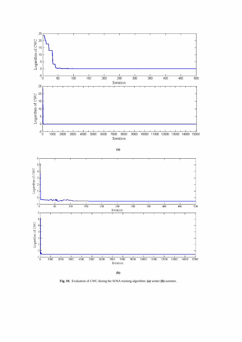
Finally, we have analyzed the convergence of CWC

along the iterations of the NN training procedure. The

behavior of CWC as a function of the iterations is shown in

Figs. 10 and 11 for SOSA and SOGA methods, respectively.

Since the CWC takes extreme values in the first iterations of

SOSA, the logarithm of CWC has been plotted in Fig.10. In

the case of SOSA, the CWC decreases gradually but non-

monotonically due to the structure of the simulated annealing

algorithm. In order to show clearly the convergence and non-

monotonicity of the SOSA method, a zoom on the behavior

of CWC has been also plotted: the upper plots in Fig. 10

show the values of CWC for the first 500 iterations. On the

contrary, from inspection of Fig.11 it is clear that CWC

decreases gradually and monotonically in the case of SOGA.

Figs. 12 and 13 show the convergence behavior of PICP

and NMPIW through the iterations of the MOGA method for

SOSA MOGA SOGA

CWC PICP NMPIW CWC PICP NMPIW CWC PICP NMPIW

0,560 0,906 0,560 0,341 0,920 0,341 0,878 0,889 0,316

0,600 0,902 0,600 0,714 0,899 0,348 0,889 0,889 0,320

0,620 0,923 0,620 0,778 0,892 0,312 1,170 0,882 0,333

0,696 0,913 0,696 0,845 0,892 0,339 1,404 0,878 0,351

0,701 0,927 0,701 0,931 0,889 0,335 1,411 0,875 0,309

0,803 0,979 0,803 1,076 0,882 0,306 1,447 0,875 0,317

0,809 0,979 0,809 1,098 0,885 0,353 1,725 0,871 0,329

0,834 0,976 0,834 1,139 0,882 0,324 1,925 0,868 0,318

0,852 0,930 0,852 1,182 0,882 0,336 2,496 0,861 0,306

1,190 0,899 0,579 1,525 0,875 0,334 2,557 0,861 0,313

2,332 0,875 0,511 1,682 0,871 0,321 2,579 0,861 0,316

5,286 0,847 0,344 2,260 0,864 0,322 2,883 0,857 0,303

8,389 0,857 0,881 2,494 0,861 0,306 3,137 0,857 0,329

8,665 0,833 0,290 2,570 0,861 0,315 4,031 0,850 0,308

37,073 0,819 0,629 2,974 0,857 0,312 4,616 0,847 0,300

53,131 0,812 0,640 4,358 0,847 0,283 6,402 0,840 0,300

144,893 0,780 0,367 5,924 0,840 0,277 6,617 0,840 0,310

525,279 0,760 0,469 6,013 0,840 0,281 7,632 0,836 0,302

7.6968e+04 0,662 0,523 6,270 0,840 0,293 9,119 0,833 0,305

4.1655e+07 0,533 0,449 7,597 0,836 0,301 10,294 0,829 0,291

the winter and summer datasets, respectively. To obtain these

graphs, we have considered the two objectives separately (as

if they were two single objectives, even if our research does

not really focus on the single-objective solutions), and we

have selected the extreme solutions on the front obtained at

each iteration. In other words, the solution giving maximum

PICP and the one giving minimum NMPIW were selected

separately. The motivation behind these last convergence

plots is to show the MOGA algorithm's ability to converge,

after a certain number of iterations, to the true optimum,

which means respectively 100% PICP and 0 NMPIW. This

happens for both the single objectives.

Table 6

Results of twenty SOSA and SOGA runs and twenty best MOGA for NN testing (summer data set).

SOSA MOGA SOGA

CWC PICP NMPIW CWC PICP NMPIW CWC PICP NMPIW

0,328 0,913 0,328 0,325 0,917 0,325 0,317 0,906 0,317

0,329 0,910 0,329 0,326 0,917 0,326 0,319 0,903 0,319

0,349 0,920 0,349 0,327 0,906 0,327 0,320 0,903 0,320

0,460 0,931 0,460 0,333 0,913 0,333 0,321 0,910 0,321

0,496 0,934 0,496 0,335 0,910 0,335 0,325 0,910 0,325

0,505 0,906 0,505 0,337 0,917 0,337 0,328 0,910 0,328

0,635 0,934 0,635 0,337 0,917 0,337 0,328 0,903 0,328

0,641 0,934 0,641 0,337 0,924 0,337 0,329 0,910 0,329

0,641 0,948 0,641 0,340 0,917 0,340 0,330 0,913 0,330

0,646 0,899 0,318 0,341 0,920 0,341 0,330 0,913 0,330

0,646 0,899 0,318 0,341 0,903 0,341 0,332 0,917 0,332

0,646 0,899 0,318 0,341 0,920 0,341 0,332 0,910 0,332

0,659 0,899 0,324 0,343 0,906 0,343 0,332 0,906 0,332

0,722 0,920 0,722 0,354 0,906 0,354 0,333 0,920 0,333

0,727 0,934 0,727 0,364 0,924 0,364 0,336 0,910 0,336

0,936 0,889 0,341 0,621 0,899 0,305 0,680 0,899 0,334

10,884 0,840 0,523 0,625 0,899 0,307 0,716 0,896 0,321

37,314 0,816 0,551 0,697 0,899 0,342 0,724 0,896 0,324

48,003 0,809 0,503 0,704 0,896 0,315 0,912 0,889 0,332

3777,362 0,733 0,877 1,537 0,872 0,298 1,322 0,878 0,336

Fig. 8. Estimated PIs for 1h ahead wind speed prediction on the testing set (dashed lines), and wind speed data included in the testing set (solid line) for

winter.

Fig. 9. Estimated PIs for 1h ahead wind speed prediction on the testing set (dashed lines), and wind speed data included in the testing set (solid line) for

summer.

(a)

(b)

Fig. 10. Evaluation of CWC during the SOSA training algorithm: (a) winter (b) summer.

(a)

(b)

Fig. 11. Evaluation of CWC during the SOGA training algorithm: (a) winter (b) summer.

(a)

(b)

Fig. 12. Evaluation of PICP and NMPIW during the MOGA training algorithm for winter period: (a) PICP (b) NMPIW.

(a)

(b)

Fig. 13. Evaluation of PICP and NMPIW during the MOGA training algorithm for summer period: (a) PICP (b) NMPIW.

6. Conclusion

Wind speed prediction is a fundamental issue for wind

power generation. The associated uncertainty needs to be

properly quantified for reliable decision making in design and

operation.

In this study, a method for the estimation of PIs by NN

has been applied for short-term wind speed prediction. Two

different time periods of historical wind speed data from

Regina, Saskatchewan, have been used to demonstrate the

NSGA-II capability of identifying NN weight values optimal

in Pareto sense, within an original multi-objective

optimization formulation of the problem of NN training. To

the knowledge of the authors, this is the first study proposing

such multi-objective formulation for the estimation of NN-

based PIs for wind speed prediction. The results obtained

confirm the validity of the proposed approach.

The application of the non-parametric Kruskal-Wallis

rank sum test to the final results obtained with SOSA, SOGA

and MOGA show that the quality of the prediction intervals

found with MOGA is superior to the one of the PIs found

using the SOSA proposed in [12], and that it is at least

comparable to the one of the PIs found using SOGA.

As for future research, the use of an ensemble of

different NNs will be considered to further increase the

accuracy of the predictions and the extension of the approach

for prediction of wind power output will be pursued.

References

[1] World Wind Energy Association, Half Year Report. Aug. 2011, 1-7.

Online, http://www.wwindea.org/home/images/stories/publications/ half_year_report_2011_wwea.pdf; Aug. 2011 [Accessed on May

2012].

[2] The European Wind Energy Association, Wind in Power 2011 European Statistics. Online, http://www.ewea.org/fileadmin/ewea_

documents/documents/publications/statistics/Stats_2011.pdf; Feb. 2012

[Accessed on May 2012]. [3] R. G. Kavasseri, K. Seetharaman, Day-ahead wind speed forecasting

using f-ARIMA models, Renewable Energy. 34 (2009) 1388-1393.

[4] X. Wang, P. Guo, X. Huang, A review of wind power forecasting models, Energy Procedia. 12 (2011) 770-778.

[5] M. Lei, L. Shiyan, J. Chuanwen, L. Hongling, Z. Yan, A review on the

forecasting of wind speed and generated power, Renewable and Sustainable Energy Reviews. 13 (2009) 915-920.

[6] R.S. Tarade, P. K. Katti, A comparative analysis for wind speed

prediction, Proceedings of International Conference on Energy,

Automation and Signal, Orissa India, Dec. 2011, pp. 556-561.

[7] A. M. Foley, P. G. Leahy, A. Marvuglia, E. J. McKeogh, Current

methods and advances in forecasting of wind power generation, Renewable Energy. 37 (2012) 1-8.

[8] W. Zhang, J. Wang, J. Wang, Z. Zhao, M. Tian, Short-term wind speed

forecasting based on a hybrid model, Applied Soft Computing. 13 (2013) 3225-3233.

[9] M. C. Alexiadis, P. S. Dokopoulos, H. S. Sahsamanoglou, Wind speed

and power forecasting based on spatial correlation models, IEEE Trans. Energy Convers. 14 (1999) 836-842.

[10] I. G. Damousis, M. C. Alexiadis, J. B. Theocharis, P. S. Dokopoulos, A

fuzzy model for wind speed prediction and power generation in wind parks using spatial correlation, IEEE Trans. Energy Convers. 19

(2004) 352- 361.

[11] A. Khosravi, S. Nahavandi, D. Creighton, A. F. Atiya, Comprehensive review of neural network-based prediction intervals and new advances,

IEEE Transactions on Neural Networks. 22 (2011) 1341-1356.

[12] A. Khosravi, S. Nahavandi, D. Creighton, A. F. Atiya, Lower upper bound estimation method for construction of neural network-based

prediction intervals, IEEE Transactions on Neural Networks. 22 (2011)

337-346. [13] A. Khosravi, S. Nahavandi, D. Creighton, A prediction interval-based

approach to determine optimal structures of neural network

metamodels, Expert Systems with Applications. 37 (2010) 2377-2387. [14] K. Deb, A. Pratap, S. Agarwal, T. Meyarivan, A fast and elitist multi-

objective genetic algorithm: NSGA-II, IEEE Transactions on

Evolutionary Computation. 6 (2002) 182-197. [15] R. Ak, Y. Li, E. Zio, Estimation of prediction intervals of neural

network models by a multi-objective genetic algorithm, Proceedings of

Flins 2012, Istanbul, Aug. 2012, pp. 1036-1041. [16] Website: http://www.weatheroffice.gc.ca/canada_e.html, (Dec., 2012).

[17] E. Zio, A study of bootstrap method for estimating the accuracy of

artificial NNs in predicting nuclear transient processes, IEEE Transactions on Nuclear Science. 53 (2006) 1460-1478.

[18] L. Yang, T. Kavli, M. Carlin, S. Clausen, P. F. M. de Groot, An

evaluation of confidence bound estimation methods for neural

networks, Proceedings of ESIT 2000, Sep. 2000, Aachen, Germany,

pp. 322-329. [19] G. Notton, C. Paoli, L. Ivanova, S. Vasileva, M. L. Nivet, Neural

network approach to estimate 10-min solar global irradiation values on

tilted planes. Renewable Energy, 50 (2013) 576-584. [20] Q. Zhou, J. Davidson, A. A. Fouad, Application of artificial neural

networks in power system security and vulnerability assessment, IEEE

Transactions on Power Systems. 9 (1994) 525-532. [21] J. M. Nazzal, I. M. El-Emary, S. A. Najim, Multilayer perceptron

neural network (MLPs) for analyzing the properties of Jordan oil shale,

World Applied Sciences Journal. 5 (2008) 546-552. [22] S. A. Kalogirou, Artificial neural networks in renewable energy

systems applications: A review, Renewable and Sustainable Energy

Reviews. 5 (2001) 373-401. [23] N. N. El-Emam, R. H. Al-Rabeh, An intelligent computing technique

for fluid flow problems using hybrid adaptive neural network and

genetic algorithm, Applied Soft Computing. 11 (2011) 3283-3296.

[24] R. Dybowski, S. J. Roberts, Confidence intervals and prediction

intervals for feed-forward neural networks, in: R. Dybowski, V. Gant

(Eds.), Clinical Applications of Artificial Neural Networks, Cambridge University Press, 2011, pp. 298- 326.

[25] D. J. C. MacKay, Bayesian interpolation, Neural Computation. 4

(1992) 415-447.

[26] C. P. I. J. Van Hinsbergen, J. W. C. Van Lint, H. J. Van Zuylen, Bayesian committee of neural networks to predict travel times with

confidence intervals, Transportation Research Part C, 17 (2009) 498-

509. [27] D. A Nix, A. S. Weigend, Estimating the mean and the variance of the

target probability distribution, Proceedings of IEEE Int. Con. Neural

Netw. World Congr. Comput. Intell., Orlondo, FL., Jun. 27 - Jul. 2, 1994, pp. 55-60.

[28] R. W. Johnson, An introduction to the bootstrap, Teaching Statistics,

23 (2001) 49-54. [29] Y. Sawaragi, H. Nakayama, T. Tanino, Theory of Multi-objective

Optimization, Orlando, FL, Academic Press Inc., 1985.

[30] A. Konak, D. W. Coit, A. E. Smith, Multi-objective optimization using genetic algorithms: a tutorial, Reliability Engineering and System

Safety. 91 (2006) 992-1007.

[31] R. Furtuna, S. Curteanu, F. Leon, Multi-objective optimization of a stacked neural network using an evolutionary hyper-heuristic, Applied

Soft Computing. 12 (2012) 133-144.

[32] E. Zitzler, L. Thiele, Multi-objective evolutionary algorithms: a comparative case study and the strength Pareto approach, IEEE

Transactions on Evolutionary Computation, 3 (1999) 257-271.

[33] N. Sirinivas, K. Deb, Multi-objective optimization using non-dominated sorting in genetic algorithms, Journal of Evolutionary

Computation. 2 (1994) 221-248.

[34] H. Mühlenbein, D. Schlierkamp-Voosen, Predictive models for the breeder genetic algorithm: I. continuous parameter optimization,

Evolutionary Computation. 1 (1993) 25-49.

[35] M. Bessaou, P. Siarry, A genetic algorithm with real-value coding to optimize multimodal continuous functions, Structural and

Multidisciplinary Optimization. 23 (2001) 63-74.

[36] M. Srinivas, L. M. Patnaik, Adaptive Probabilities of crossover and mutation in genetic algorithms, IEEE Transactions on Systems, Man

and Cybernetics. 24 (1994) 656-667.

[37] Z. Michalewicz, Genetic Algorithms + Data Structures = Evolution

Programs, Springer-Verlag, New York, 1992.

[38] Canadian Wind Energy Association (CanWEA), Media Kit 2012.

Online, http://www.canwea.ca/pdf/windsight/CanWEA_MediaKit.pdf; 2012 [Accessed on May 2012].

[39] SaskPower Annual Report 2011. Online, http://www.saskpower.com/ news_publications/assets/annual_reports/2011_skpower_annual_report.

pdf; 2011 [Accessed on May 2012].

[40] J.L. Rodgers, W.A. Nicewander, Thirteen ways to look at the correlation coefficient, The American Statistician. 42 (1988) 59-66.

[41] M. Hollander, D. A. Wolfe, Nonparametric Statistical Methods, John

Wiley & Sons, New York, 1973. [42] T. Hastie, R. Tibshirani, J. Friedman, The elements of Statistical

Learning: Data Mining, Inference and Prediction, second ed., Springer,

2008. [43] R. Karki, P. Hu, R. Billinton, A simplified wind power generation

model for reliability evaluation, IEEE Transactions on Energy

Conversion. 21 (2006) 533-540. [44] N.L. Buccola, T.M. Wood, Empirical models of wind conditions on

upper Klamath lake, Oregon, Scientific Investigations Report 2010-

5201, Online, http://pubs.usgs.gov/sir/2010/5201/pdf/sir20105201.pdf; 2010, [Accessed on May 2012].

[45] G. E. P. Box, G. M. Jenkins, G. C. Reinsel, Time Series Analysis,

Forecasting and Control, fourth ed., Wiley, 2008. [46] E. Zio, P. Baraldi, and N. Pedroni, Optimal power system generation

scheduling by multi-objective genetic algorithms with preferences,

Reliability Engineering and System Safety. 94 (2009) 432-444. [47] S. Bandyopadhyay, S. Saha, U. Maulik, K. Deb, A Simulated

annealing-based multi-objective optimization algorithm: AMOSA.

IEEE Transactions on Evolutionary Computation. 12 (2008) 269-283. [48] E. L. Ulungu, J. Teghem, Ch. Ost, Efficiency of interactive multi-

objective simulated annealing through a case study, Journal of the

Operational Research Society. 49 (1998) 1044-1050. [49] R. A. Johnson, D. W. Wichern, Applied Multivariate Statistical

Analysis, fifth ed., Pearson Education Inc., 2002.

[50] D. F. Bauer, Constructing confidence sets using rank statistics, Journal of the American Statistical Association. 67 (1972) 687–690.

Ronay Ak received the B.Sc. degree in mathematical

engineering from Yildiz Technical University, Istanbul,

Turkey, in 2004 and the M.Sc. degree in industrial engineering from Istanbul Technical University,

Istanbul, Turkey in 2009. She is currently pursuing the

Ph.D. degree at Chair on Systems Science and the Energetic Challenge, European Foundation for New

Energy-Électricité de France (EDF), École Centrale

Paris (ECP) and École Superieure d’Électricité (SUPELEC), France, since March 2011. Her research interests include uncertainty quantification,

prediction methods, artificial intelligence, reliability analysis of wind-

integrated power networks and optimization heuristics.

Yanfu Li is an Assistant Professor at Ecole Centrale Paris (ECP) & Ecole Superieure d'Electricite

(SUPELEC), Paris, France. Dr. Li completed his PhD

research in 2009 at National University of Singapore, and went to the University of Tennessee as a research

associate. His current research interests include

reliability modeling, uncertainty analysis, evolutionary computing, and Monte Carlo simulation. He is the

author of more than 30 publications, all in refereed international journals,

conferences, and books. He is an invited reviewer of over 10 international journals.

Valeria Vitelli received the B. Sc. and the M. Sc.

degrees in mathematical engineering from Politecnico di

Milano, Milan, Italy, in 2006 and 2008, respectively. She received the Ph.D. degree in Mathematical Models

and Methods for Engineering, with a focus on statistical

models for classification of high-dimensional data, in May 2012. She worked as a postdoc researcher within

the Chair on Systems Science and the Energetic

Challenge, European Foundation for New Energy- Électricité de France

(EDF), École Centrale Paris (ECP) and École Superieure d’Électricité

(SUPELEC), France, from February 2012 to May 2013.

Enrico Zio received the Ph.D. degree in nuclear engineering from Politecnico di Milano and MIT in

1995 and 1998, respectively. He is currently Director of

the Chair on Systems Science and the Energetic Challenge, European Foundation for New Energy-

Électricité de France (EDF), at École Centrale Paris

(ECP) and École Superieure d’Électricité (SUPELEC) and full professor at Politecnico di Milano. His research

focuses on the characterization and modeling of the

failure/repair/maintenance behavior of components, complex systems and their reliability, availability, maintainability, prognostics, safety,

vulnerability and security, advanced Monte Carlo simulation methods, soft

computing techniques and optimization heuristics.