multi-objective fuzzy optimization & fuzzy zdt … · certificate this is to certify that the...

DEPARTMENT OF MATHEMATICS

INDIAN INSTITUTE OF TECHNOLOGY, KHARAGPUR

Thesis for the degree of

Masters of Science in

Mathematics & Computing

Under esteemed guidance of

Prof. D. Chakraborty Department Of Mathematics

Submitted By: VIKASH KUMAR

(05MA2001) May’10

MU

LTI-

OB

JEC

TIV

E F

UZ

ZY

OP

TIM

IZA

TIO

N

FUZ

ZY

GE

NE

TIC

ALG

OR

ITH

MS

& F

UZ

ZY

ZD

T T

EST

FU

NC

TIO

NS

ACKNOWLEDGEMENT

I express my sincere gratitude to my supervisor, respected Prof. Debjani Chakraborty under whose supervision and guidance this work has been carried out. Without her whole hearted involvement, advice, support and constant encouragement, it would have been impossible to carry out this project work with confidence.

I am grateful to Prof. N. Chakraborti (Department of Metallurgical and Materials Engineering) for his constant guidance and Mr. Abhay Kumar (M.Sc. in Mathematics, Mathematics and Computing) for his help and encouragement in finishing the work in the given time frame.

I am indebted to the Department of Mathematics and Department of Metallurgical & Materials Engineering, IIT Kharagpur for extending help and facilities.

VIKASH KUMAR (05MA2001)



CERTIFICATE

This is to certify that the thesis entitled “Optimizing fuzzy multi‐objective problems using fuzzy genetic algorithms, FZDT test functions” is a bonafide work carried out by Mr. Vikash Kumar (05MA2001) under my supervision and guidance for partial fulfillment of the requirements for the degree of Master of Science in Mathematics from Department of Mathematics, Indian Institute of Technology, Kharagpur.

Prof. Debjani Chakraborty

DEPARTMENT OF MATHEMATICS INDIAN INSTITUTE OF TECHNOLOGY, KHARAGPUR

Submitted By:

VIKASH KUMAR (05MA2001)



Contents

PREFACE

1

1. Prologue

1.1. Introduction 2 1.2. Literature Review 2 1.3. Objectives 3

2. Fuzzy Number

2.1. Fuzzy Sets 4 2.2. Fuzzy Numbers 4

2.2.1. Generalized Fuzzy Number 4 2.2.2. Triangular Fuzzy Number 5 2.2.3. Trapezoidal Fuzzy Number 5

2.3. Algebraic operators 5 2.4. Trigonometric operators 6 2.5. Graded Mean Integration (GMI) 6

3. Genetic Algorithms

3.1. Genetic Algorithms(GA) 8 3.2. Fitness function 9 3.3. Genetic Search Process 9 3.4. GA Operators 9

3.4.1. Reproduction 9 3.4.2. Crossover 10 3.4.3. Mutation 11

3.5. Genetic Algorithm framework 11 3.6. NMGA: The New Multi‐objective Genetic Algorithm 11

3.6.1. Discretization of Functional Space 12 3.6.2. The Neighborhood and the recombination process 13 3.6.3. Ranking the Population 14 3.6.4. Rank Based Population Sizing 14

3.7. NSGA II 15 3.7.1. Population Initialization 16 3.7.2. Non‐dominated sort 16 3.7.3. Crowding distance 17 3.7.4. Selection 17 3.7.5. Genetic Operator 18

3.7.5.1. Simulated Binary Crossover 18 3.7.5.2. Polynomial Mutation 18

3.7.6. Recombination & Selection 19

4. Performance Measures and Test Functions of GA

4.1. Performance Measures 20 4.2. Test Functions 20

4.2.1. ZDT1 21 4.2.2. ZDT2 21 4.2.3. ZDT3 21 4.2.4. ZDT4 21 4.2.5. ZDT5 22 4.2.6. ZDT6 22

5. Solution Strategy: Fuzzy Genetic Algorithm

5.1. Problem Formulation 24 5.2. Fuzzy optimization problem 24 5.3. Fuzzy Genetic Algorithm 24

5.3.1. FGA Framework 24 5.3.2. Initialization 25 5.3.3. Genetic Operators: Mutation & Crossover 25 5.3.4. Fuzzy Ranking 25 5.3.5. Graded Mean Integration 26 5.3.6. Advanced Concepts 26

6. Test functions of FGA

6.1. FZDT 27

7. Experimentation and Results

7.1. FNMGA 29 7.1.1. Discretization of Functional Space 29 7.1.2. The Neighborhood and the recombination process 29 7.1.3. Ranking the Population 29 7.1.4. Rank Based Population Sizing 30 7.1.5. Results 31

7.2. FNSGA II 34 7.2.1. Population Initialization 35 7.2.2. Non‐dominated sort 35 7.2.3. Crowding distance 35 7.2.4. Selection 36 7.2.5. Genetic Operator 36

7.2.5.1. Simulated Binary Crossover 36 7.2.5.2. Polynomial Mutation 37

7.2.6. Recombination & Selection 37 7.2.7. Results 37

7.3. Comparative Study of the two FGA: FNMGA & FNSGA II 40

8. Conclusion 42

REFERENCES

43

1

1 Preface

The following work outlines a robust method for accounting the fuzziness of the objective space while solving the real world optimization problems. Use of mean/approximated value of input parameters doesn't account for the variability in the optimized solution inherited due to variability in the input parameters which is very crucial, especially in real world problems. Accounting the fuzziness of the variable space transforms a multi‐objective optimization problem to a multi‐objective fuzzy optimization problem. Previous attempts to solve fuzzy optimization problem tries to remodel the fuzzy optimization problems into real valued optimization problems using mathematical reductions/transformations, extension principle, interval arithmetic etc and hence solve them using traditional approach. Thus killing valuable information concealed in the fuzziness of the problem and hence destroying the essence of the problem.

The following work describes and evaluates a unique solution strategy for optimizing fuzzy multi‐objective problems by integrating genetic algorithms with concepts of fuzzy logic. The unique way of problem formulation required no tweaking in genetic operators of mutation and crossover but the concept of ranking has been carefully extended to fuzzy domain. The standard benchmark test function, ZDT[4], have been extrapolated to fuzzy domain as FZDT and proposed to be benchmark test function for fuzzy optimization algorithms. The results have been successfully verified with FZDT test functions and were found coherent with ZDT test functions under classical assumptions.

2

Chapter 1 Prologue

1.1 Introduction

Multi objective optimization problem is the process of simultaneously optimizing two or more conflicting objectives subject to certain constraints. Such problems can be found in various fields: product and process design, finance, aircraft design, the oil and gas industry, automobile design, or wherever optimal decisions need to be taken in the presence of trade‐offs between two or more conflicting objectives. Genetic algorithms are a particular class of evolutionary algorithms that use techniques inspired by evolutionary biology such as inheritance, mutation, selection, and crossover and is the most commonly used search techniques in computing to find exact or approximate solutions to such optimization and search problems.

In real world problems, parameters of a process are never precisely fixed to a definite value. Transients, noise, measurement errors, Instrument’s least count etc makes it even more difficult to know their exact value at any time stamp. Even if externally regulated, parameters have some variability in their values. This variability has been continuously ignored by using mean/approximated/fixed value of the parameters thus losing the precious information about the variability in the final optimized solution.

For example, in an isothermal process, temperature is externally controlled at a certain fixed level. In general, for calculations or optimizations, temperature is taken constant at that specified level. But, there is always variability or fuzziness about the fixed value in such controlled parameters which needs to be preserved and reflected in the final results.

1.2 Literature review

There exists a number of works attempting to solve the fuzzy optimization problem. However almost all the previous approach tries to remodel the fuzzy optimization problems into crisp real optimization problems and hence solve them using traditional approach. Ribeiro. R. A. and F. M. Pires [10] discussed a fuzzy linear programming using simulated annealing algorithm. The work outlines a simulated annealing algorithm which provides a simple tool for solving fuzzy optimization problem. Often the issue is not how to fuzzify or remove the conceptual impression, but which tool enables simple solutions for these intrinsically uncertain problems.

Bucklet et al. [11] showed that it is possible to train a layered feed forward neural net, which with certain sign restriction on its weights gives approximates solution to the fuzzy optimization problem. Buckley and feuring [12] applied the evolutionary algorithm to two classical fully fuzzified programs to show that It can produce good approximate results.

3

Jamison and lodwick [7] proposed a penalty method for characterizing the constant violation to formulate the problem as an unconstrained fuzzy optimization problem. The objective is them redefined as optimizing the expected midpoint of the image of the fuzzify function.

Wang and Wang [8] transformed the fuzzy linear programming problem into a multiobjective problem with parametric interval valued multiobjective linear programming problem.

Chiang [9] used statistical data to formulate statistical confidence interval and to derive interval valued fuzzy numbers. Then the estimated value of the constraint coefficient is generated to form a flexible linear programming problem.

1.3 Objectives

Following work focuses on solving multi‐objective fuzzy optimization problem addressing the concerns mentioned above. Our approach can be broken down into following objectives:

1. Multi objective fuzzy optimization problem formulation and mapping real variable space to fuzzy decision space.

2. Extend the ZDT functions (FZDT) to make them compatible with fuzzy environment. 3. Develop Fuzzy Genetic Algorithm working from a real variable space to fuzzy decision

space and test it using the extended FZDT functions.

4

2 Chapter 2 Fuzzy Number

2.1 Fuzzy Sets

If X is a collection of objects denoted generically by x then a fuzzy set A in X is a set of ordered pairs: Ã= {(x, μÃ(x)) / x є X} where μÃ(x) is called the membership function or grade of membership of x in Ã which maps X to the membership space M .The range of the membership function is a subset of the nonnegative real numbers whose supremum is finite. Elements with a zero degree of membership are normally not listed.

2.2 Fuzzy Numbers

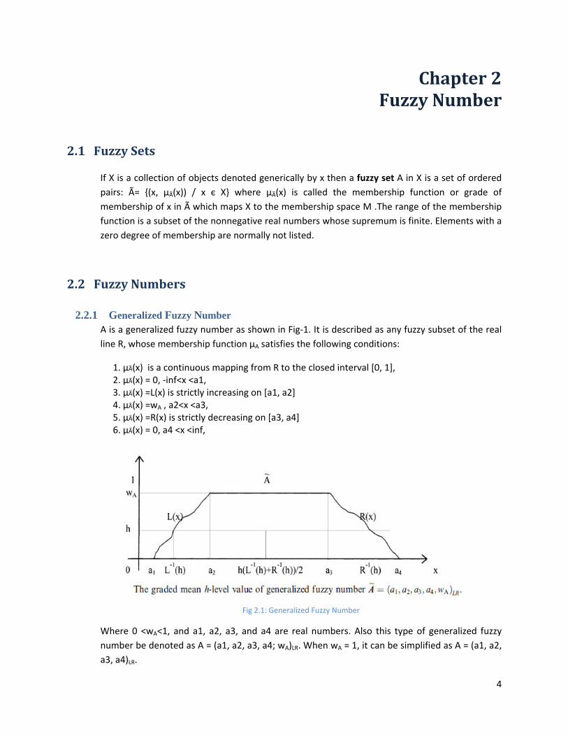
2.2.1 Generalized Fuzzy Number A is a generalized fuzzy number as shown in Fig‐1. It is described as any fuzzy subset of the real line R, whose membership function μA satisfies the following conditions:

1. μÃ(x) is a continuous mapping from R to the closed interval [0, 1], 2. μÃ(x) = 0, ‐inf<x <a1, 3. μÃ(x) =L(x) is strictly increasing on [a1, a2] 4. μÃ(x) =wA , a2<x <a3, 5. μÃ(x) =R(x) is strictly decreasing on [a3, a4] 6. μÃ(x) = 0, a4 <x <inf,

Fig 2.1: Generalized Fuzzy Number

Where 0 <wA<1, and a1, a2, a3, and a4 are real numbers. Also this type of generalized fuzzy number be denoted as A = (a1, a2, a3, a4; wA)LR. When wA = 1, it can be simplified as A = (a1, a2, a3, a4)LR.

5

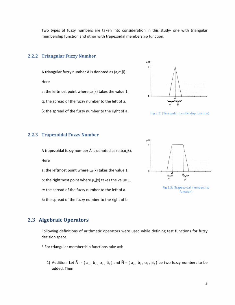
Two types of fuzzy numbers are taken into consideration in this study‐ one with triangular membership function and other with trapezoidal membership function.

2.2.2 Triangular Fuzzy Number

A triangular fuzzy number Ã is denoted as (a,α,β).

Here

a: the leftmost point where μÃ(x) takes the value 1.

α: the spread of the fuzzy number to the left of a.

β: the spread of the fuzzy number to the right of a.

Fig 2.2: (Triangular membership function)

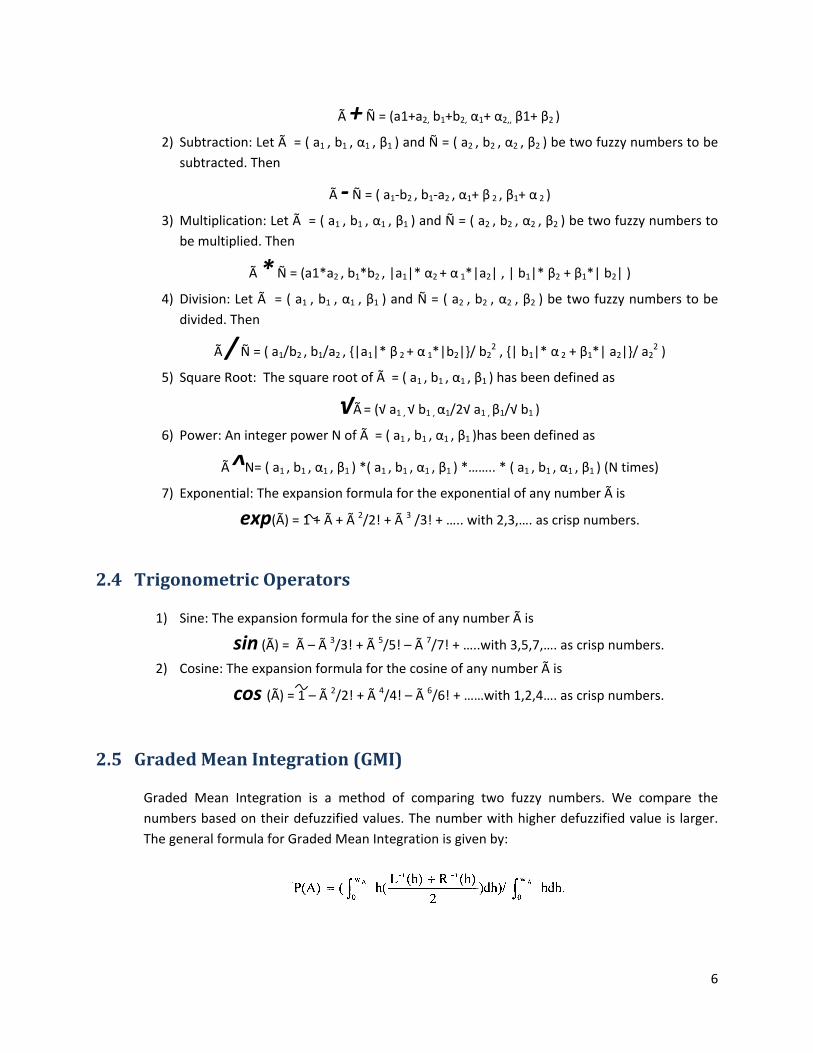
2.2.3 Trapezoidal Fuzzy Number

A trapezoidal fuzzy number Ã is denoted as (a,b,α,β).

Here

a: the leftmost point where μÃ(x) takes the value 1.

b: the rightmost point where μÃ(x) takes the value 1.

α: the spread of the fuzzy number to the left of a.

β: the spread of the fuzzy number to the right of b.

Fig 2.3: (Trapezoidal membership function)

2.3 Algebraic Operators

Following definitions of arithmetic operators were used while defining test functions for fuzzy decision space.

* For triangular membership functions take a=b.

1) Addition: Let Ã = ( a1 , b1 , α1 , β1 ) and Ñ = ( a2 , b2 , α2 , β2 ) be two fuzzy numbers to be

added. Then

6

Ã + Ñ = (a1+a2, b1+b2, α1+ α2,, β1+ β2 )

2) Subtraction: Let Ã = ( a1 , b1 , α1 , β1 ) and Ñ = ( a2 , b2 , α2 , β2 ) be two fuzzy numbers to be subtracted. Then

Ã ‐ Ñ = ( a1‐b2 , b1‐a2 , α1+ β 2 , β1+ α 2 )

3) Multiplication: Let Ã = ( a1 , b1 , α1 , β1 ) and Ñ = ( a2 , b2 , α2 , β2 ) be two fuzzy numbers to be multiplied. Then

Ã * Ñ = (a1*a2 , b1*b2 , |a1|* α2 + α 1*|a2| , | b1|* β2 + β1*| b2| )

4) Division: Let Ã = ( a1 , b1 , α1 , β1 ) and Ñ = ( a2 , b2 , α2 , β2 ) be two fuzzy numbers to be divided. Then

Ã / Ñ = ( a1/b2 , b1/a2 , {|a1|* β 2 + α 1*|b2|}/ b22 , {| b1|* α 2 + β1*| a2|}/ a2

2 )

5) Square Root: The square root of Ã = ( a1 , b1 , α1 , β1 ) has been defined as

√Ã = (√ a1 , √ b1 , α1/2√ a1 , β1/√ b1 )

6) Power: An integer power N of Ã = ( a1 , b1 , α1 , β1 )has been defined as

Ã ^N= ( a1 , b1 , α1 , β1 ) *( a1 , b1 , α1 , β1 ) *…….. * ( a1 , b1 , α1 , β1 ) (N times)

7) Exponential: The expansion formula for the exponential of any number Ã is

exp(Ã) = 1 + Ã + Ã 2/2! + Ã 3 /3! + ….. with 2,3,…. as crisp numbers.

2.4 Trigonometric Operators

1) Sine: The expansion formula for the sine of any number Ã is

sin (Ã) = Ã – Ã 3/3! + Ã 5/5! – Ã 7/7! + …..with 3,5,7,…. as crisp numbers.

2) Cosine: The expansion formula for the cosine of any number Ã is

cos (Ã) = 1 – Ã 2/2! + Ã 4/4! – Ã 6/6! + ……with 1,2,4…. as crisp numbers.

2.5 Graded Mean Integration (GMI)

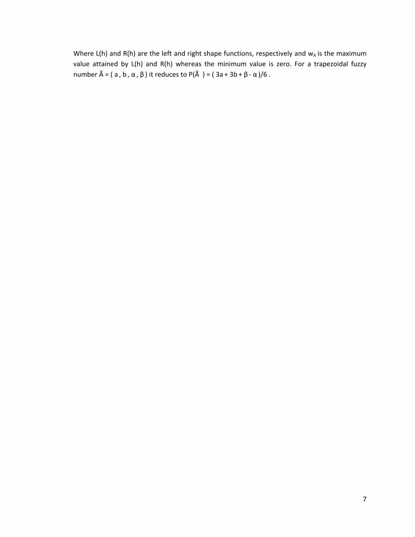
Graded Mean Integration is a method of comparing two fuzzy numbers. We compare the numbers based on their defuzzified values. The number with higher defuzzified value is larger. The general formula for Graded Mean Integration is given by:

7

Where L(h) and R(h) are the left and right shape functions, respectively and wA is the maximum value attained by L(h) and R(h) whereas the minimum value is zero. For a trapezoidal fuzzy number Ã = ( a , b , α , β ) it reduces to P(Ã ) = ( 3a + 3b + β ‐ α )/6 .

8

3 Chapter 3 Genetic Algorithms

3.1 Genetic Algorithms (GA)

Genetic Algorithms are probabilistic search algorithms which simulate natural evolution. In these algorithms the search space of a problem is represented as a collection of individuals. These individuals are represented by character strings or matrices which are often referred to as chromosomes. The purpose of using a genetic algorithm is to find the individual from the search space with the best “genetic material”. The quality of an individual is measured with an evaluation function. The part of the search space to be examined is called the population.

First, the initial population is chosen, and the quality of this population is determined. Next, in every iteration, parents are selected from the population. These parents produce children which are added to the population. For all newly created individuals of the resulting population a probability near to zero exists that they will “mutate” i.e. that they will change their hereditary distinctions. After that, some individuals are removed from the population according to a selection criterion in order to reduce the population to its initial size. One iteration of the algorithm is referred to as a generation.

The operators which define the child production process and the mutation process are called the crossover operator and the mutation operator respectively. Mutation and crossover play different roles in the genetic algorithm. Mutation is needed to explore new states and helps the algorithm to avoid local optima. Crossover should increase the average quality of the population. By choosing adequate crossover and mutation operators, the probability that the genetic algorithm results in a near optimal solution in a reasonable number of iterations is increased. There can be various criteria for stopping AGA. For example, if it is possible to determine previously the number of iterations needed.

A typical genetic algorithm requires two things to be defined:

1. A genetic representation of the solution domain, 2. A fitness function to evaluate the solution domain.

A standard representation of the solution is as an array of bits. Arrays of other types and structures can be used in essentially the same way. The main property that makes these genetic representations convenient is that their parts are easily aligned due to their fixed size, that facilitates simple crossover operation. Variable length representations were also used, but crossover implementation is more complex in this case. Tree‐like representations are explored in Genetic programming.

9

3.2 Fitness Function

A fitness function is a particular type of objective function that quantifies the optimality of a solution. The fitness function is defined over the genetic representation and measures the quality of the represented solution. The fitness function is always problem dependent. For instance, in the knapsack problem we want to maximize the total value of objects that we can put in a knapsack of some fixed capacity. A representation of a solution might be an array of bits, where each bit represents a different object, and the value of the bit (0 or 1) represents whether or not the object is in the knapsack. Not every such representation is valid, as the size of objects may exceed the capacity of the knapsack. The fitness of the solution is the sum of values of all objects in the knapsack if the representation is valid, 1or 0 otherwise. In some problems, it is hard or even impossible to define the fitness expression; in these cases, interactive genetic algorithms are used. To achieve maximization, a fitness function F(x) is first derived from the problem’s objective function f(x) and one sets F(x) = f(x). For minimization, several transformations are possible. One popular transformation is

F(x) = 1/(1+f(x))

This transformation does not alter the location of the minimum, but it converts the original minimization problem into a maximization problem.

3.3 Genetic Search Process

GAs begin with a population of randomly selected initial solutions – a population of random strings representing the problem’s decision variables {xi}. Thereafter, each of these initially picked strings is evaluated to find its fitness. If a satisfactory solution (based on some acceptability or search stoppage criterion) is already at hand, the search is stopped. If not, the initial population is subjected to genetic evolution to procreate the next generation of candidate solutions. The genetic process of procreation uses the initial population as the input. The members of the population are “processed” by three main GA operators – reproduction, crossover and mutation to create the progenies (the next generation of candidate solutions to the optimization problem at hand). The progenies are then evaluated and tested for termination. If the termination criterion is not met, the three GA operators iteratively operate upon the population. The procedure is continued till the termination criterion is met. One cycle (iteration) of these operations to produce offspring is called a generation in the GA terminology.

3.4 GA operators

3.4.1 Reproduction This is usually the first operator that is applied to an existing population to create progenies. Reproduction first select good parent solutions or strings to form the mating pool. The essential

10

idea in reproduction is to select strings of above average fitness from the existing population and insert their multiple copies in the mating pool, in a probabilistic manner. This results in a selection of existing solutions with better than average fitness to act as parents for the next generation. One popular reproduction operator uses fitness proportionate selection in which a parent solution is selected to move to the mating pool with a probability that is proportional to its own fitness. Thus, the ith parent would be selected randomly with a probability pi proportional to fi, given by

Pi= fi /Σfi Treated in this manner, a solution that has a high fitness will have a higher probability of being copied into the mating pool and thus participate in parenting offspring. On the other hand, a solution with a smaller fitness value will have a smaller probability of being copied into the mating pool.

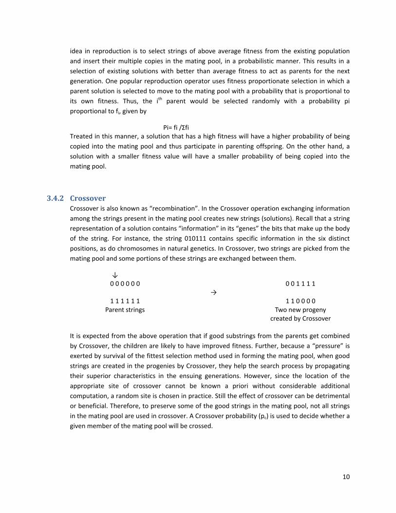
3.4.2 Crossover Crossover is also known as “recombination”. In the Crossover operation exchanging information among the strings present in the mating pool creates new strings (solutions). Recall that a string representation of a solution contains “information” in its “genes” the bits that make up the body of the string. For instance, the string 010111 contains specific information in the six distinct positions, as do chromosomes in natural genetics. In Crossover, two strings are picked from the mating pool and some portions of these strings are exchanged between them.

↓ 0 0 0 0 0 0

1 1 1 1 1 1

Parent strings

→

0 0 1 1 1 1

1 1 0 0 0 0

Two new progeny created by Crossover

It is expected from the above operation that if good substrings from the parents get combined by Crossover, the children are likely to have improved fitness. Further, because a “pressure” is exerted by survival of the fittest selection method used in forming the mating pool, when good strings are created in the progenies by Crossover, they help the search process by propagating their superior characteristics in the ensuing generations. However, since the location of the appropriate site of crossover cannot be known a priori without considerable additional computation, a random site is chosen in practice. Still the effect of crossover can be detrimental or beneficial. Therefore, to preserve some of the good strings in the mating pool, not all strings in the mating pool are used in crossover. A Crossover probability (pc) is used to decide whether a given member of the mating pool will be crossed.

11

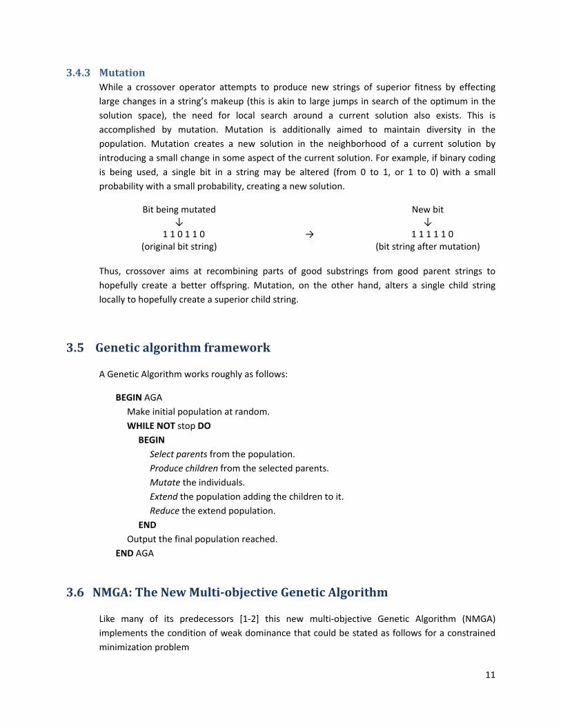
3.4.3 Mutation While a crossover operator attempts to produce new strings of superior fitness by effecting large changes in a string’s makeup (this is akin to large jumps in search of the optimum in the solution space), the need for local search around a current solution also exists. This is accomplished by mutation. Mutation is additionally aimed to maintain diversity in the population. Mutation creates a new solution in the neighborhood of a current solution by introducing a small change in some aspect of the current solution. For example, if binary coding is being used, a single bit in a string may be altered (from 0 to 1, or 1 to 0) with a small probability with a small probability, creating a new solution.

Bit being mutated ↓

1 1 0 1 1 0 (original bit string)

→

New bit ↓

1 1 1 1 1 0 (bit string after mutation)

Thus, crossover aims at recombining parts of good substrings from good parent strings to hopefully create a better offspring. Mutation, on the other hand, alters a single child string locally to hopefully create a superior child string.

3.5 Genetic algorithm framework

A Genetic Algorithm works roughly as follows:

BEGIN AGA Make initial population at random. WHILE NOT stop DO BEGIN Select parents from the population. Produce children from the selected parents. Mutate the individuals. Extend the population adding the children to it. Reduce the extend population. END Output the final population reached. END AGA

3.6 NMGA: The New Multiobjective Genetic Algorithm

Like many of its predecessors [1‐2] this new multi‐objective Genetic Algorithm (NMGA) implements the condition of weak dominance that could be stated as follows for a constrained minimization problem

12

Minimize Objective Functions: fi(X) i = 1, 2,….., I

Subject to Constraints: gj(X) j = 1, 2,.…., J

Where X = (xk : k = 1,2,…..,K) is a K‐tuple vector of variables,

Let an I‐tuple vector of objectives is defined as: Ωi = (f i: i= 1, 2,…., I)

Then the condition for dominance between any two objective vectors can be taken as:

In other words, if one particular solution is at least as good, or better in terms of all the objective functions, when compared to another solution, and definitely better in terms of at least one objective function, it is considered to be a weakly dominating solution.

In NMGA this condition has been implemented in a discretized functional space. Further details are provided below.

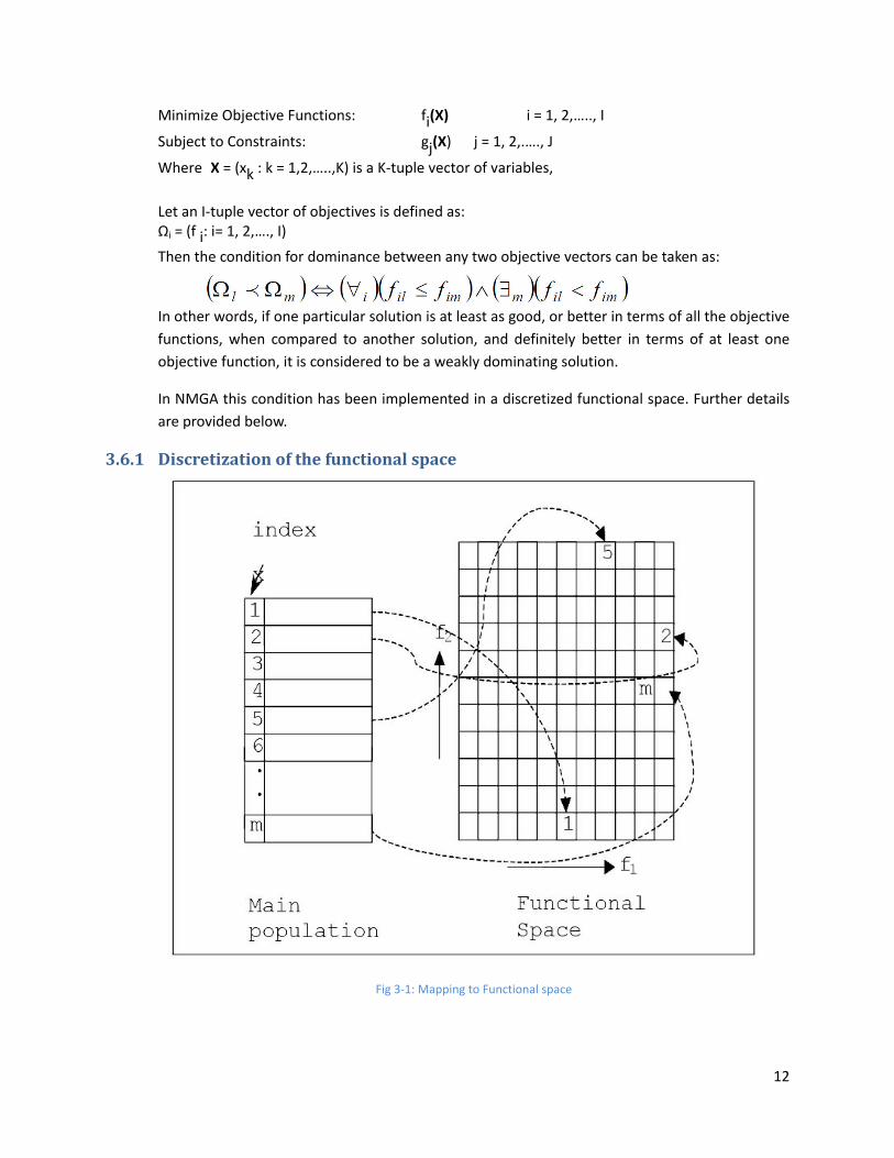
3.6.1 Discretization of the functional space

Fig 3‐1: Mapping to Functional space

13

In this algorithm a traditional Genetic Algorithm population is mapped on to the functional space, as demonstrated in Figure 3.1

Each member is assigned to a discrete grid in the function space. For a system of I objective functions, the index of the grid can be designated through an integer coordinate system (g1, g2, ….. gI), related to the corresponding objective functions as:

Where the subscripts indicate the lower and upper bounds of the function and n denotes the total number of grids that the user needs to specify. A particular grid location, in principle, can be inhabited by more than one members of the population, provided they have got identical indices.

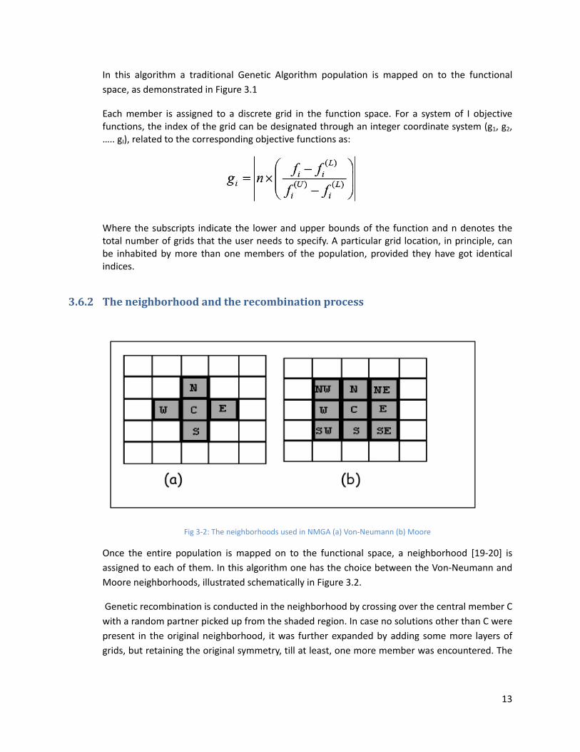
3.6.2 The neighborhood and the recombination process

Fig 3‐2: The neighborhoods used in NMGA (a) Von‐Neumann (b) Moore

Once the entire population is mapped on to the functional space, a neighborhood [19‐20] is assigned to each of them. In this algorithm one has the choice between the Von‐Neumann and Moore neighborhoods, illustrated schematically in Figure 3.2.

Genetic recombination is conducted in the neighborhood by crossing over the central member C with a random partner picked up from the shaded region. In case no solutions other than C were present in the original neighborhood, it was further expanded by adding some more layers of grids, but retaining the original symmetry, till at least, one more member was encountered. The

14

children are also placed in the functional space, and subsequently, a pruning of the population takes place, as detailed below.

3.6.3 Ranking the population Once the genetic recombination and mutation gets over, all the dominated individuals in the neighborhood are deleted. The resulting population is then ranked, following either the Goldberg [21] or the Fonseca [22] approach. In the former, the non‐dominated members of the population are taken out of the population as rank 1. The truncated population is again checked for dominance and the non‐dominated set is once again removed out of it, this time as rank 2 members, and the procedure continues. In the Fonseca [22] strategy the entire population is checked for dominance and the ranks to the individuals are assigned using the formula:

Ri= 1 +Nd where Ri is the rank of the individual i, and Nd is the number of individuals that dominate it. In this study The Fonseca approach was preferred as it reduces the computational burden. The population is further downsized, based upon the rank information, as detailed below.

3.6.4 Rank based population sizing Since NMGA keeps both the parents and the children in the main population, the population size tends to grow, often unmanageably, even after removing the dominated solutions in the neighborhood. Based upon the rank information, the population is therefore trimmed further, and the procedure adopted is as follows:

The main idea behind this population sizing procedure is to ensure that all types of members are present in the final set of size S that the member specifies. Initially all the individuals are ranked using the Fonseca and Fleming strategy and the permitted number of individuals in the final set is computed by the function:

NR = N0 *e‐R

Here, NR denotes the permitted number of individuals of rank R, N0 is a constant calculated using the value of S. There is no upper limit on the value of rank and so, in principle, we can assume that the maximum rank is infinity while the lowest, by definition, is unity. The individuals having the rank of ‘1’ constitute the Pareto‐front. The total set should be equal to the sum of the permitted number of individuals of all ranks, such that

S = N1 + N2 + N3 + …… N∞

Substituting the values of N1, N2, N3 …… N∞into the above equation, the final equation becomes:

S = N0 * (e‐1 + e‐2 + … +e‐∞)

Summing the infinite series in geometric progression, the value of is calculated as:

N0 = S * (e‐1)

Hinbean

Thsh

3.7 NS

Nocoshso

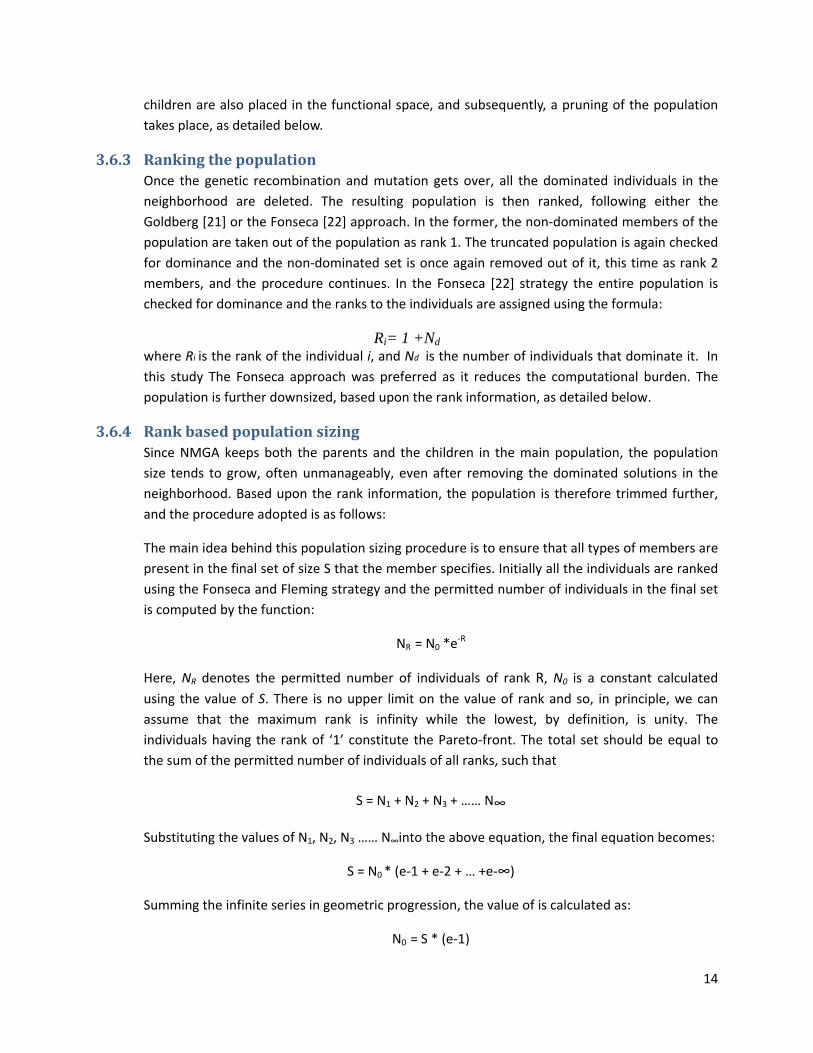
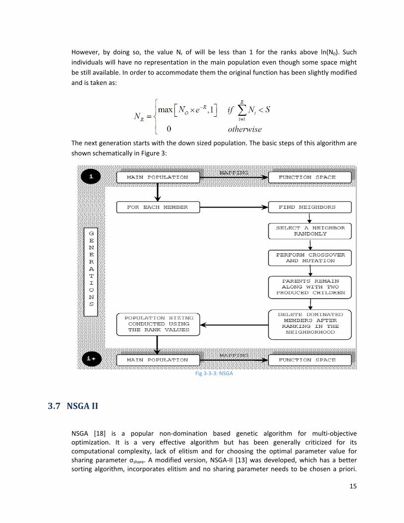
owever, by ndividuals wile still availabnd is taken as

he next genehown schema

SGA II

SGA [18] iptimization. omputationaharing paramorting algorit

doing so, thel have no reple. In order tos:

ration starts atically in Figu

s a populaIt is a verl complexity,

meter σshare. Ahm, incorpor

e value Nr opresentation o accommod

with the dowure 3:

r non‐dominry effective , lack of elitiA modified verates elitism

of will be lesin the main ate them the

wn sized popu

Fig 3‐3‐3: NSG

nation basealgorithm bism and for ersion, NSGAand no shari

s than 1 forpopulation e

e original func

ulation. The b

GA

d genetic abut has beechoosing the‐II [13] was ding paramete

the ranks aeven though ction has bee

basic steps of

algorithm fon generally e optimal padeveloped, wer needs to b

above ln(N0). some space n slightly mo

f this algorith

or multi‐objecriticized forameter valuwhich has a bbe chosen a p

15

Such might dified

m are

ective or its ue for better priori.

16

The initialized population is sorted based on non‐domination into each front. The first front being completely non‐dominant set in the current population and the second front being dominated by the individuals in the first front only and the front goes so on. Each individual in the each front are assigned rank (fitness) values or based on front in which they belong to. Individuals in first front are given a fitness value of 1 and individuals in second are assigned fitness value as 2 and so on. In addition to fitness value a new parameter called crowding distance is calculated for each individual. The crowding distance is a measure of how close an individual is to its neighbors. Large average crowding distance will result in better diversity in the population. Parents are selected from the population by using binary tournament selection based on the rank and crowding distance. An individual is selected in the rank is lesser than the other or if crowding distance is greater than the other 1. The selected population generates offspring from crossover and mutation operators. The population with the current population and current offspring is sorted again based on non‐domination and only the best N individuals are selected, where N is the population size. The selection is based on rank and the on crowding distance on the last front.

3.7.1 Population Initialization The population is initialized based on the problem range and constraints if any.

3.7.2 NonDominated sort The initialized population is sorted based on non‐domination. An individual is said to dominate another if the objective functions of it is no worse than the other and at least in one of its objective functions it is better than the other. The fast sort algorithm [16] is described as below for each

for each individual p in main population P do the following • Initialize Sp = Ø. This set would contain all the individuals that is being dominated by p. • Initialize np = 0. This would be the number of individuals that dominate p. • for each individual q in P

- if p dominated q then add q to the set Sp i.e. Sp = Sp U {q} - else if q dominates p then increment the domination counter for p i.e. np = np +

1 • If np = 0 i.e. no individuals dominate p then p belongs to the first front; Set rank of individual

p to one i.e prank = 1. Update the first front set by adding p to front one i.e F1 = F1 U {p} This is carried out for all the individuals in main population P.

Initialize the front counter to one. i = 1 Following is carried out while the ith front is nonempty i.e. Fi ≠ Ø • Q = Ø. The set for storing the individuals for (i + 1)th front. • for each individual p in front Fi

- for each individual q in Sp (Sp is the set of individuals dominated by p) nq = nq¡1, decrement the domination count for individual q.

if nq = 0 then none of the individuals in the subsequent fronts would

dominate q. Hence set qrank = i + 1. Update the set Q with individual q

i.e. Q = Q U {q}. - Increment the front counter by one.

17

- Now the set Q is the next front and hence Fi = Q. This algorithm is better than the original NSGA ([5]) since it utilize the information about the set that an individual dominate (Sp) and number of individuals that dominate the individual (np).

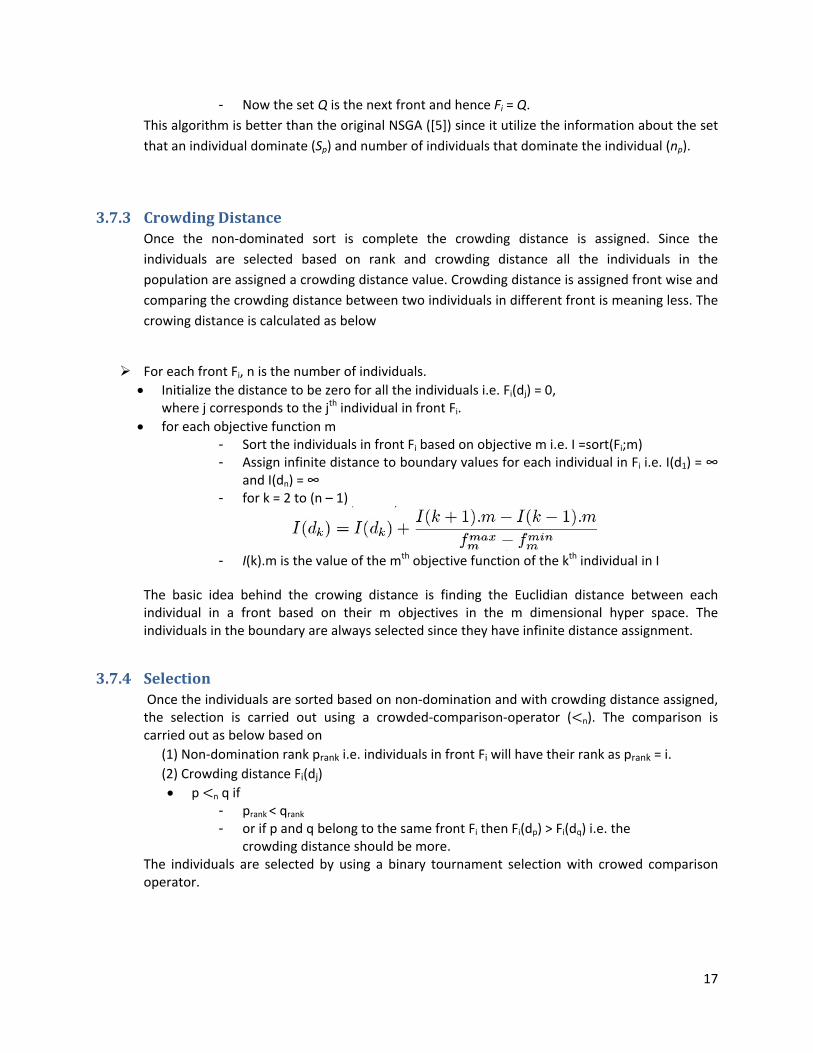
3.7.3 Crowding Distance Once the non‐dominated sort is complete the crowding distance is assigned. Since the individuals are selected based on rank and crowding distance all the individuals in the population are assigned a crowding distance value. Crowding distance is assigned front wise and comparing the crowding distance between two individuals in different front is meaning less. The crowing distance is calculated as below

For each front Fi, n is the number of individuals. • Initialize the distance to be zero for all the individuals i.e. Fi(dj) = 0,

where j corresponds to the jth individual in front Fi. • for each objective function m

- Sort the individuals in front Fi based on objective m i.e. I =sort(Fi;m) - Assign infinite distance to boundary values for each individual in Fi i.e. I(d1) = ∞

and I(dn) = ∞ - for k = 2 to (n – 1)

- I(k).m is the value of the mth objective function of the kth individual in I

The basic idea behind the crowing distance is finding the Euclidian distance between each individual in a front based on their m objectives in the m dimensional hyper space. The individuals in the boundary are always selected since they have infinite distance assignment.

3.7.4 Selection Once the individuals are sorted based on non‐domination and with crowding distance assigned, the selection is carried out using a crowded‐comparison‐operator ( n). The comparison is carried out as below based on

(1) Non‐domination rank prank i.e. individuals in front Fi will have their rank as prank = i. (2) Crowding distance Fi(dj) • p n q if

- prank < qrank - or if p and q belong to the same front Fi then Fi(dp) > Fi(dq) i.e. the

crowding distance should be more. The individuals are selected by using a binary tournament selection with crowed comparison operator.

18

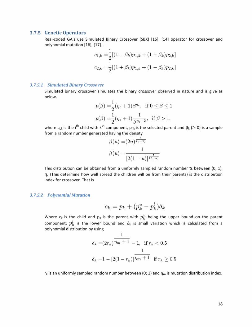
3.7.5 Genetic Operators Real‐coded GA's use Simulated Binary Crossover (SBX) [15], [14] operator for crossover and polynomial mutation [16], [17].

3.7.5.1 Simulated Binary Crossover Simulated binary crossover simulates the binary crossover observed in nature and is give as below.

where ci,k is the i

th child with kth component, pi,k is the selected parent and βk ( 0) is a sample from a random number generated having the density

This distribution can be obtained from a uniformly sampled random number between (0, 1). ηc (This determine how well spread the children will be from their parents) is the distribution index for crossover. That is

3.7.5.2 Polynomial Mutation

Where ck is the child and pk is the parent with being the upper bound on the parent component, is the lower bound and δk is small variation which is calculated from a polynomial distribution by using

rk is an uniformly sampled random number between (0; 1) and ηm is mutation distribution index.

19

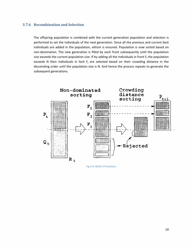
3.7.6 Recombination and Selection

The offspring population is combined with the current generation population and selection is performed to set the individuals of the next generation. Since all the previous and current best individuals are added in the population, elitism is ensured. Population is now sorted based on non‐domination. The new generation is filled by each front subsequently until the population size exceeds the current population size. If by adding all the individuals in front Fj the population exceeds N then individuals in font Fj are selected based on their crowding distance in the descending order until the population size is N. And hence the process repeats to generate the subsequent generations.

Fig 3‐4: NSGA II Procedure

20

4 Chapter 4 Performance measures &Test functions of GA

4.1 Performance measures

Evaluating and comparing different optimization techniques experimentally always involves the notion of performance. In the case of multiobjective optimization, the definition of quality is substantially more complex than for single‐objective optimization problems, because the optimization goal itself consists of multiple objectives:

1. The distance of the resulting nondominated set to the Pareto‐optimal front should be minimized.

2. A good (in most cases uniform) distribution of the solutions found is desirable. The assessment of this criterion might be based on a certain distance metric.

3. The extent of the obtained nondominated front should be maximized, i.e., for each objective, a wide range of values should be covered by the nondominated solutions.

Deb (1999) identified several features that may cause difficulties for multiobjective EAs in

1) Converging to the Pareto‐optimal front 2) Maintaining diversity within the population.

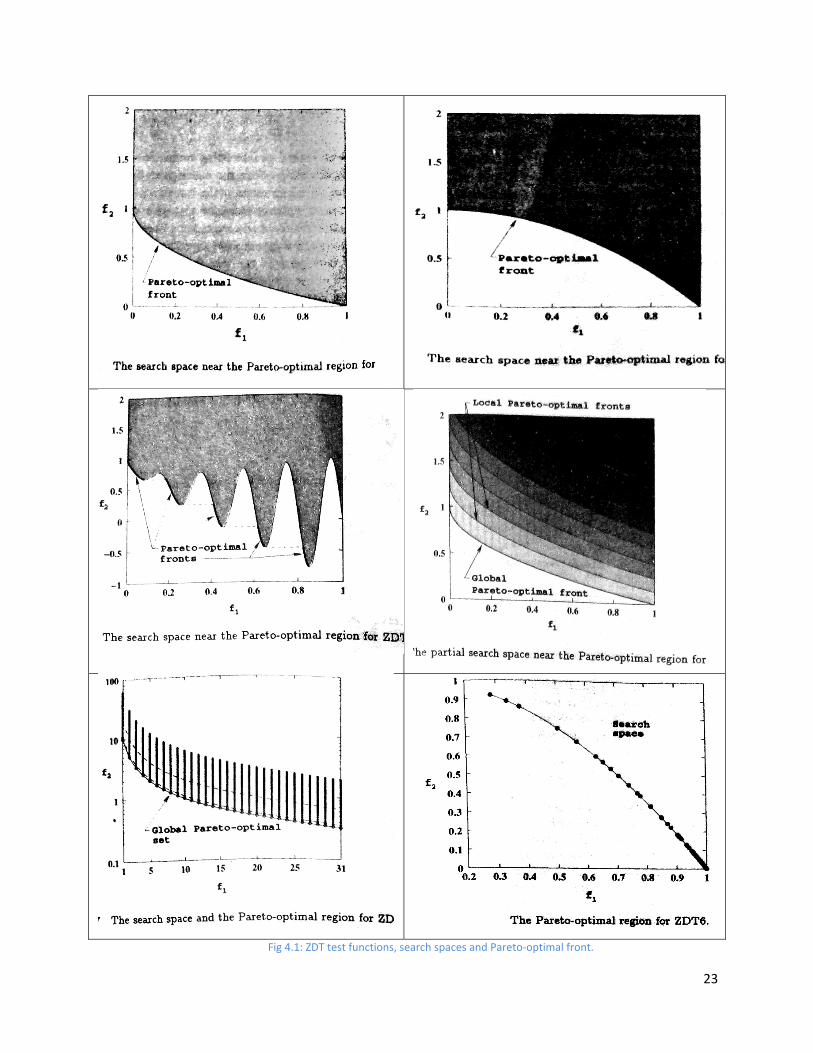
Concerning the first issue, multimodality, deception, and isolated optima are well‐known problem areas in single‐objective evolutionary optimization. The second issue is important in order to achieve a well distributed nondominated front. However, certain characteristics of the Pareto‐optimal front may prevent an EA from finding diverse Pareto‐ optimal solutions: convexity or nonconvexity, discreteness, and nonuniformity. For each of the six problems features mentioned, a corresponding test function, called ZDT Test Function, was constructed following the guidelines in Deb (1999).

4.2 Test functions

Functions belonging to the ZDT series of test functions [] are well known benchmark functions for testing GA. These functions checks the convergence and scalability of a GA on parameters like: Convex/Non convex optimal fonts, Continuous/Discontinuous fonts, Sparsely/Densely populated fonts etc. Each of the test functions defined below is structured in the same manner and consists itself of three functions: f, g and h

21

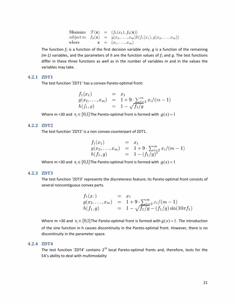
The function f1 is a function of the first decision variable only, g is a function of the remaining (m‐1) variables, and the parameters of h are the function values of f1 and g. The test functions differ in these three functions as well as in the number of variables m and in the values the variables may take.

4.2.1 ZDT1 The test function ’ZDT1’ 1has a convex Pareto‐optimal front:

Where m =30 and ]1,0[∈ix The Pareto‐optimal front is formed with 1)( =xg

4.2.2 ZDT2 The test function ’ZDT2’ is a non convex counterpart of ZDT1.

Where m =30 and ]1,0[∈ix The Pareto‐optimal front is formed with 1)( =xg

4.2.3 ZDT3 The test function ‘ZDT3’ represents the discreteness feature; its Pareto‐optimal front consists of several noncontiguous convex parts.

Where m =30 and ]1,0[∈ix The Pareto‐optimal front is formed with 1)( =xg . The introduction

of the sine function in h causes discontinuity in the Pareto‐optimal front. However, there is no discontinuity in the parameter space.

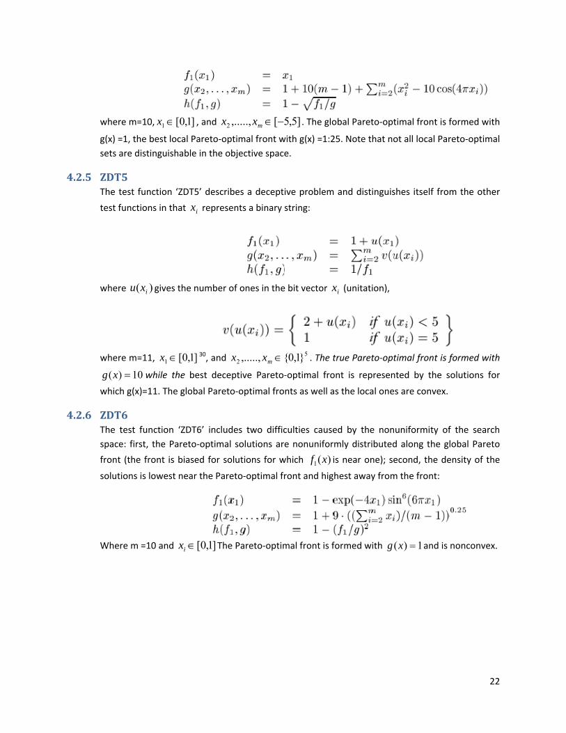
4.2.4 ZDT4 The test function ‘ZDT4’ contains 219 local Pareto‐optimal fronts and, therefore, tests for the EA’s ability to deal with multimodality

22

where m=10, ]1,0[1 ∈x , and ]5,5[,.....,2 −∈mxx . The global Pareto‐optimal front is formed with

g(x) =1, the best local Pareto‐optimal front with g(x) =1:25. Note that not all local Pareto‐optimal sets are distinguishable in the objective space.

4.2.5 ZDT5 The test function ‘ZDT5’ describes a deceptive problem and distinguishes itself from the other

test functions in that ix represents a binary string:

where )( ixu gives the number of ones in the bit vector ix (unitation),

where m=11, ]1,0[1 ∈x 30, and 5

2 }1,0{,....., ∈mxx . The true Pareto‐optimal front is formed with

10)( =xg while the best deceptive Pareto‐optimal front is represented by the solutions for

which g(x)=11. The global Pareto‐optimal fronts as well as the local ones are convex.

4.2.6 ZDT6 The test function ‘ZDT6’ includes two difficulties caused by the nonuniformity of the search space: first, the Pareto‐optimal solutions are nonuniformly distributed along the global Pareto

front (the front is biased for solutions for which )(1 xf is near one); second, the density of the

solutions is lowest near the Pareto‐optimal front and highest away from the front:

Where m =10 and ]1,0[∈ix The Pareto‐optimal front is formed with 1)( =xg and is nonconvex.

23

Fig 4.1: ZDT test functions, search spaces and Pareto‐optimal front.

24

5 Chapter 5 Solution strategy:

Fuzzy genetic algorithm

5.1 Problem Formulation

In real world problems, the input parameters of an optimization problem inherit variability due to external factors. Variability of such parameters is being accounted by taking them fuzzy in nature about the mean/fixed value. The membership function of such parameters can easily be determined by repetitive observations and by analyzing extensive data set. Decision variable however are assumed to be crisp real numbers. Thus our result accounts and reflects the variability of the plug‐in parameters while fixing the decision variable at exact values. Since the optimization problem aims to determine the optimized value of decision variables (with no inherent variability) based on the information concealed within the input parameters (with inherent variability) and the objective space. This completely justifies our assumption of taking decision variables to be crisp real numbers and input parameters as fuzzy numbers.

5.2 Fuzzy Optimization Problem

A multi‐objective fuzzy constrained optimization problem can be represented as:

Minimize Objective Functions: fi(A,X) i = 1, 2,….., I (1)

Subject to Constraints: gj(A,X) j = 1, 2,.…., J (2)

Where A = (xm : m = 1,2,…..,M) is a M‐tuple vector of fuzzy variables,

X = (an : n = 1,2,…...,N) is a N‐tuple vector of decision variables,

As per the problem formulation, decision space is a fuzzy space and the fi's and gi's are fuzzy numbers.

5.3 Fuzzy genetic algorithm (FGA)

5.3.1 FGA Framework FGA follows the basic framework of a genetic algorithm. BEGIN FGA

25

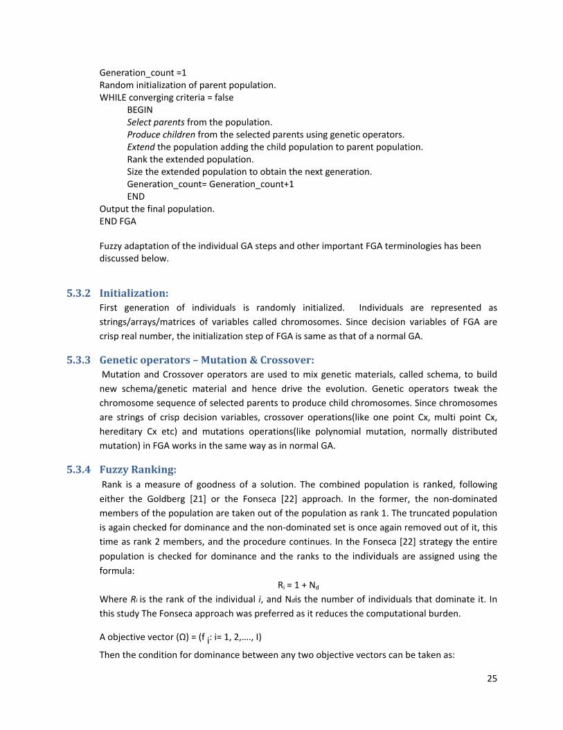
Generation_count =1 Random initialization of parent population. WHILE converging criteria = false

BEGIN Select parents from the population. Produce children from the selected parents using genetic operators. Extend the population adding the child population to parent population. Rank the extended population. Size the extended population to obtain the next generation. Generation_count= Generation_count+1 END

Output the final population. END FGA Fuzzy adaptation of the individual GA steps and other important FGA terminologies has been discussed below.

5.3.2 Initialization: First generation of individuals is randomly initialized. Individuals are represented as strings/arrays/matrices of variables called chromosomes. Since decision variables of FGA are crisp real number, the initialization step of FGA is same as that of a normal GA.

5.3.3 Genetic operators – Mutation & Crossover: Mutation and Crossover operators are used to mix genetic materials, called schema, to build new schema/genetic material and hence drive the evolution. Genetic operators tweak the chromosome sequence of selected parents to produce child chromosomes. Since chromosomes are strings of crisp decision variables, crossover operations(like one point Cx, multi point Cx, hereditary Cx etc) and mutations operations(like polynomial mutation, normally distributed mutation) in FGA works in the same way as in normal GA.

5.3.4 Fuzzy Ranking: Rank is a measure of goodness of a solution. The combined population is ranked, following either the Goldberg [21] or the Fonseca [22] approach. In the former, the non‐dominated members of the population are taken out of the population as rank 1. The truncated population is again checked for dominance and the non‐dominated set is once again removed out of it, this time as rank 2 members, and the procedure continues. In the Fonseca [22] strategy the entire

population is checked for dominance and the ranks to the individuals are assigned using the formula:

Ri = 1 + Nd Where Ri is the rank of the individual i, and Ndis the number of individuals that dominate it. In this study The Fonseca approach was preferred as it reduces the computational burden.

A objective vector (Ω) = (f i: i= 1, 2,…., I)

Then the condition for dominance between any two objective vectors can be taken as:

26

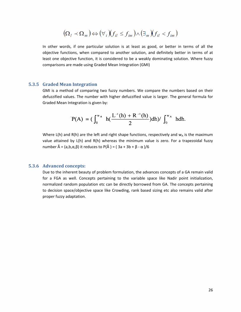
In other words, if one particular solution is at least as good, or better in terms of all the objective functions, when compared to another solution, and definitely better in terms of at least one objective function, it is considered to be a weakly dominating solution. Where fuzzy comparisons are made using Graded Mean Integration (GMI)

5.3.5 Graded Mean Integration GMI is a method of comparing two fuzzy numbers. We compare the numbers based on their defuzzified values. The number with higher defuzzified value is larger. The general formula for Graded Mean Integration is given by:

Where L(h) and R(h) are the left and right shape functions, respectively and wA is the maximum value attained by L(h) and R(h) whereas the minimum value is zero. For a trapezoidal fuzzy number Ã = (a,b,α,β) it reduces to P(Ã ) = ( 3a + 3b + β ‐ α )/6

5.3.6 Advanced concepts: Due to the inherent beauty of problem formulation, the advances concepts of a GA remain valid for a FGA as well. Concepts pertaining to the variable space like Nadir point initialization, normalized random population etc can be directly borrowed from GA. The concepts pertaining to decision space/objective space like Crowding, rank based sizing etc also remains valid after proper fuzzy adaptation.

6.1 FZ

FZco

Th

MM

Usif1

Table 6. Function

FZDT1

FZDT2

FZDT3

ZDT

ZDT test funconvergence a

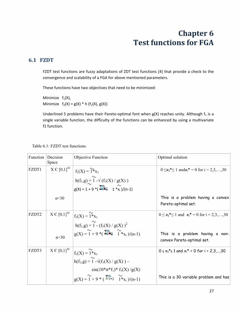
hese function

Minimize f1(XMinimize f2(X

nderlined 5 pngle variable1 function.

.1: FZDT test

Decision Space

X Є [0,1]3

n=30

X Є [0,1]3

n=30

X Є [0,1]3

ctions are fuzand scalability

ns have two o

X), X) = g(X) * h (f

problems have function, th

t functions.

Objective

30 f1(X) =

h(f1,g) =

g(X) = 1 +

0 f1(X) = 1

h(f1,g) =

g(X) = 1

0

f1(X) = 1

h(f1,g) =

g(X) = 1

zzy adaptatioy of a FGA for

objectives tha

f1(X), g(X))

ve their Parete difficulty o

e Function

1*x1

= 1 -√ (f1(X)

9 *( 1

1*x1

= 1 - (f1(X) /

+ 9 *(

1*x1

1 -√(f1(X) /

sin(10*π*f1

+ 9 * (

T

ons of ZDT ter above ment

at need to be

to‐optimal fof the function

/ g(X) )

1 *xi )/(n‐1)

g(X) )2

1 *xi )/(n-

g(X) ) –

1)* f1(X) /g(X

1*xi )/(n-

Test fun

st functions [ioned parame

minimized:

nt when g(X)ns can be en

O

-1)

X)

-1)

6 Cnction

[4] that proveters.

) reaches unithanced by us

Optimal solut

0 ≤x1*≤ 1 an

This is a Pareto-opti

0 ≤ x1*≤ 1 an

This is a convex Pare

0 ≤ x1*≤ 1 and

This is a 30

Chaptes for F

ide a check t

ty. Although sing a multiva

tion

ndxi* = 0 for

problem havimal set.

nd xi* = 0 for

problem haeto-optimal s

d xi* = 0 for

variable pro

27

r 6 GA

to the

f1 is a ariate

i = 2,3,…,30

ving a conve

r i = 2,3,…,30

aving a nonset.

i = 2,3,…,30

oblem and ha

ex

0

n-

as

FZDT4

FZDT6

Atausp

Fo

n=30

X Є [0,1]x[–5,5

n=10

X Є [0,1]1

n=10

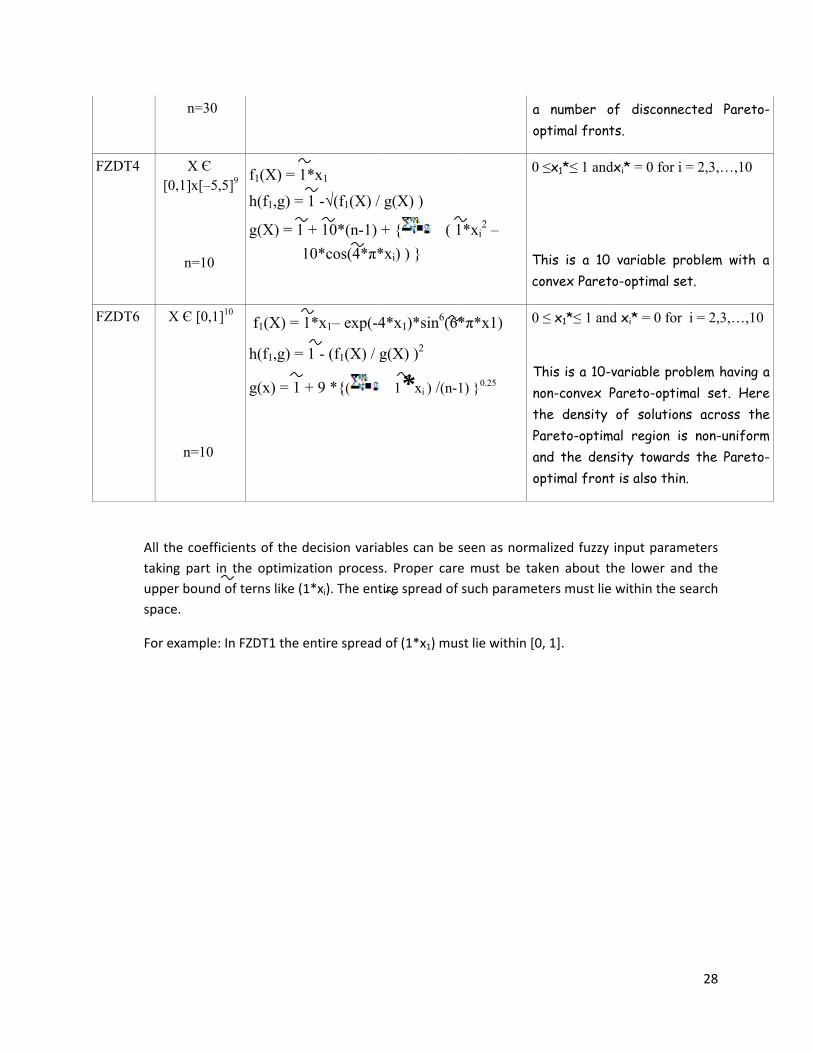
ll the coefficaking part in pper bound opace.

or example: I

]9 f1(X) = 1

h(f1,g) =

g(X) = 1 1

0 f1(X) =

h(f1,g) =

g(x) = 1

ients of the dthe optimiza

of terns like (1

n FZDT1 the e

1*x1

1 -√(f1(X) /

+ 10*(n-1) 10*cos(4*π*

1*x1– exp(-4

1 - (f1(X) / g

+ 9 *{(

decision variaation process1*xi). The ent

entire spread

g(X) )

+ { ( *xi) ) }

4*x1)*sin6(6

g(X) )2

1*xi ) /(n-

ables can be s. Proper cartire spread of

d of (1*x1) mu

1*xi2 –

0

6*π*x1)

-1) }0.25

0

seen as normre must be taf such parame

ust lie within [

a number ooptimal fron

0 ≤x1*≤ 1 and

This is a 10convex Paret

0 ≤ x1*≤ 1 an

This is a 10-non-convex the density Pareto-optimand the denoptimal fron

malized fuzzyaken about teters must lie

[0, 1].

of disconnets.

dxi* = 0 for i

0 variable prto-optimal se

nd xi* = 0 for

-variable proPareto-optim of solution

mal region isnsity towardst is also thin

y input paramthe lower ane within the s

28

cted Pareto

= 2,3,…,10

roblem with et.

i = 2,3,…,10

oblem having mal set. Herns across ths non-uniforms the Pareto

n.

meters d the earch

o-

a

0

a re he m o-

29

7 Chapter 7 Experimentation and Results

Based on the FGA framework discussed above, two real coded algorithms are developed: FMSGA and FNSGA. These algorithms are fuzzy adaptations of two very effective GAs: NSGA [7a] & NMGA [7b].

7.1 FNMGA

7.1.1 Discretization of the functional space In this algorithm a traditional Genetic Algorithm population is mapped on to the functional space. Each member is assigned to a discrete grid in the function space. For a system of I objective functions, the index of the grid can be designated through an integer coordinate system (g1,g2, …gi), related to the corresponding objective functions as:

Where, ‘ denotes defuzzified values, the subscripts indicate the lower and upper bounds of the function and n denotes the total number of grids that the user needs to specify. A particular grid location, in principle, can be inhabited by more than one members of the population, provided they have got identical indices.

7.1.2 The neighborhood and the recombination process Once the entire population is mapped on to the functional space, a Moore neighborhood [19‐20] is assigned to each of them. Genetic recombination is conducted in the neighborhood by crossing over the central member C with a random partner picked up from the Moore neighborhood. In case no solutions other than C were present in the original neighborhood, it was further expanded by adding some more layers of grids, but retaining the original symmetry, till at least, one more member was encountered. The children are also placed in the functional space, and subsequently, a pruning of the population takes place.

7.1.3 Ranking the population Once the genetic recombination and mutation gets over, all the dominated individuals in the

neighborhood are deleted. The resulting population is then ranked, following Fonseca [22]

30

approach. In the Fonseca strategy the entire population is checked for dominance by fuzzy comparison using GMI approach as discussed in section 3.2.4 &3.2.5 and the ranks to the

individuals are assigned using the formula:

Ri= 1 +Nd Where Ri is the rank of the individual i, and Nd is the number of individuals that dominate it.

7.1.4 Rank based population sizing The main idea behind this population sizing procedure is to ensure that all types of members are present in the final set of size that the member specifies. Initially all the individuals are ranked using the Fonseca and Fleming strategy and the permitted number of individuals in the final set is computed by the function: S

NR = N0 *e-R Here, NR denotes the permitted number of individuals of rank R, N0 is a constant calculated using the value of S. There is no upper limit on the value of rank and so, in principle, we can assume that the maximum rank is infinity while the lowest, by definition, is unity. The individuals having the rank of ‘1’ constitute the Pareto‐front. The total set should be equal to the sum of the permitted number of individuals of all ranks, such that

S = N1 + N2 + N3 + …… N∞

Substituting the values of N1, N2, N3 …… N∞ into the above equation, the final equation becomes

S = N0 * (e‐1 + e‐2 + … +e‐∞)

Summing the infinite series in geometric progression, the value of is calculated as

N0 = S * (e-1) However, by doing so, the value Nr of will be less than 1 for the ranks above ln(N0). Such individuals will have no representation in the main population even though some space might be still available. In order to accommodate them the original function has been slightly modified and is taken as:

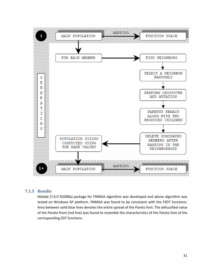
The next generation starts with the down sized population. The basic steps of this algorithm are shown schematically in Figure 3.

31

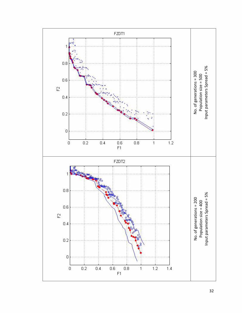
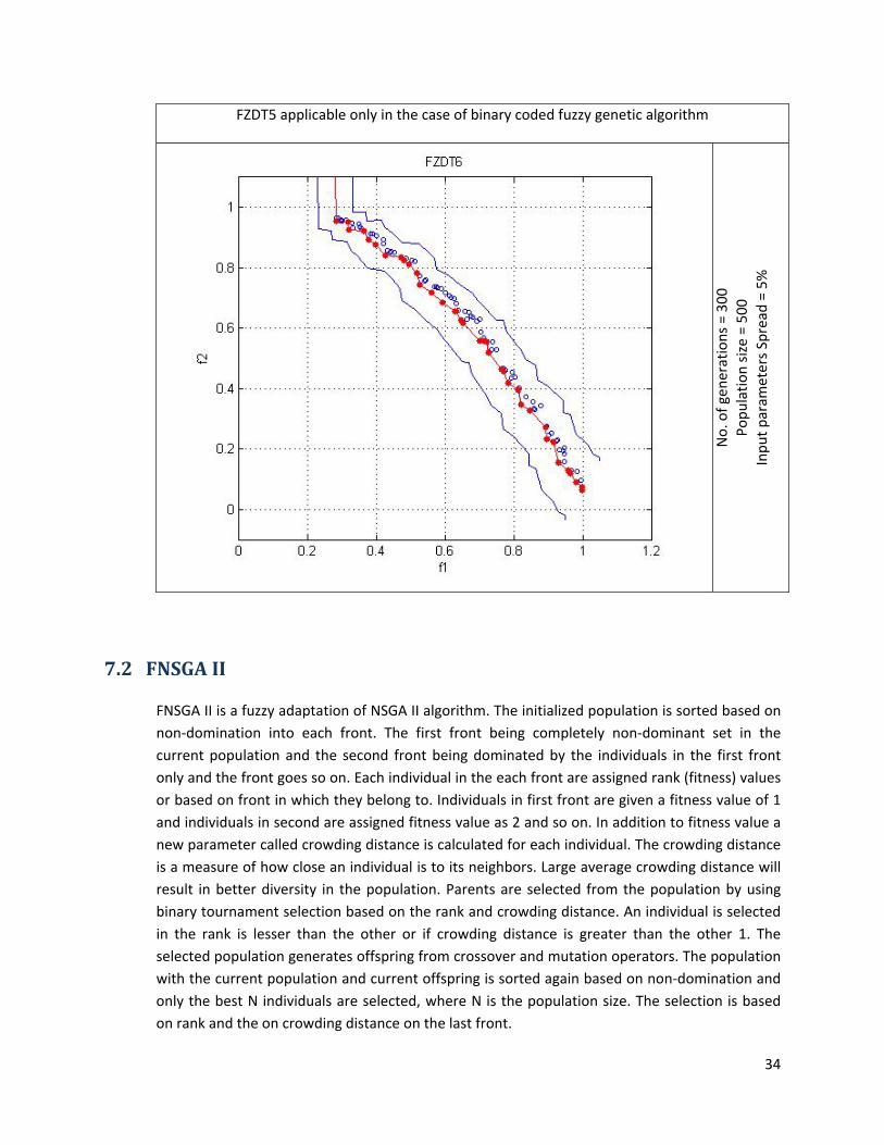
7.1.5 Results Matlab (7.6.0 R2008a) package for FNMGA algorithm was developed and above algorithm was tested on Windows XP platform. FNMGA was found to be consistent with the FZDT functions. Area between solid blue lines denotes the entire spread of the Pareto font. The defuzzified value of the Pareto front (red line) was found to resemble the characteristics of the Pareto font of the corresponding ZDT functions.

32

No. of gen

erations = 300

Po

pulatio

n size = 500

Inpu

t param

eters Spread

= 5%

No. of gen

erations = 200

Po

pulatio

n size = 400

Inpu

t param

eters Spread

= 5%

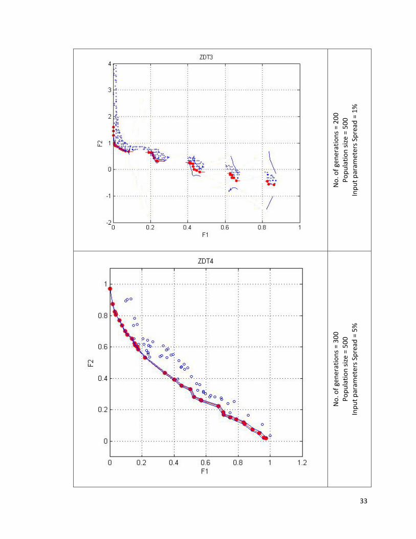
33

No. of gen

erations = 200

Po

pulatio

n size = 500

Inpu

t param

eters Spread

= 1%

No. of gen

erations = 300

Po

pulatio

n size = 500

Inpu

t param

eters Spread

= 5%

34

FZDT5 applicable only in the case of binary coded fuzzy genetic algorithm

No. of gen

erations = 300

Po

pulatio

n size = 500

Inpu

t param

eters Spread

= 5%

7.2 FNSGA II

FNSGA II is a fuzzy adaptation of NSGA II algorithm. The initialized population is sorted based on non‐domination into each front. The first front being completely non‐dominant set in the current population and the second front being dominated by the individuals in the first front only and the front goes so on. Each individual in the each front are assigned rank (fitness) values or based on front in which they belong to. Individuals in first front are given a fitness value of 1 and individuals in second are assigned fitness value as 2 and so on. In addition to fitness value a new parameter called crowding distance is calculated for each individual. The crowding distance is a measure of how close an individual is to its neighbors. Large average crowding distance will result in better diversity in the population. Parents are selected from the population by using binary tournament selection based on the rank and crowding distance. An individual is selected in the rank is lesser than the other or if crowding distance is greater than the other 1. The selected population generates offspring from crossover and mutation operators. The population with the current population and current offspring is sorted again based on non‐domination and only the best N individuals are selected, where N is the population size. The selection is based on rank and the on crowding distance on the last front.

35

7.2.1 Population Initialization The population of real variables is initialized based on the problem range and constraints if any.

7.2.2 NonDominated sort The initialized population is sorted based on non‐domination by fuzzy comparisons using GMI approach (discussed in section 1.8). An individual is said to dominate another if the objective functions of it is no worse than the other and at least in one of its objective functions it is better than the other. The fast sort algorithm [16] is described as below for each

for each individual p in main population P do the following • Initialize Sp = Ø. This set would contain all the individuals that are being dominated by p. • Initialize np = 0. This would be the number of individuals that dominate p. • for each individual q in P

- if p dominated q then add q to the set Sp i.e. Sp = Sp U {q} - else if q dominates p then increment the domination counter for p ( np = np +1)

• If np = 0 i.e. no individuals dominate p then p belongs to the first front; Set rank of individual p to one i.e prank = 1. Update the first front set by adding p to front one i.e F1 = F1 U {p}

This is carried out for all the individuals in main population P.

Initialize the front counter to one. i = 1 Following is carried out while the ith front is nonempty i.e. Fi ≠ Ø • Q = Ø. The set for storing the individuals for (i + 1)th front. • for each individual p in front Fi

- for each individual q in Sp (Sp is the set of individuals dominated by p) nq = nq¡1, decrement the domination count for individual q. if nq = 0 then none of the individuals in the subsequent fronts would dominate q. Hence set qrank = i + 1. Update the set Q with individual q i.e. Q = Q U {q}.

- Increment the front counter by one. - Now the set Q is the next front and hence Fi = Q.

This algorithm is better than the original NSGA ([5]) since it utilize the information about the set that an individual dominate (Sp) and number of individuals that dominate the individual (np).

7.2.3 Crowding Distance Once the non‐dominated sort is complete the crowding distance is assigned. Since the individuals are selected based on rank and crowding distance all the individuals in the population are assigned a crowding distance value. Crowding distance is assigned front wise and comparing the crowding distance between two individuals in different front is meaning less. The crowing distance is calculated as below

For each front Fi, n is the number of individuals. • Initialize the distance to be zero for all the individuals i.e. Fi(dj) = 0,

where j corresponds to the jth individual in front Fi. • for each objective function m

36

- Sort(using GMI approach) the individuals in front Fi based on objective m i.e. I =sort(Fi;m)

- Assign infinite distance to boundary values for each individual in Fi i.e. I(d1) = ∞ and I(dn) = ∞

- for k = 2 to (n – 1)

- I(k).m is the value of the mth objective function of the kth individual in I

The basic idea behind the crowing distance is finding the Euclidian distance between each individual in a front based on their m objectives in the m dimensional hyper space. The individuals in the boundary are always selected since they have infinite distance assignment.

7.2.4 Selection Once the individuals are sorted based on non‐domination and with crowding distance assigned, the selection is carried out using a crowded‐comparison‐operator ( n). The comparison is carried out as below based on

(1) Non‐domination rank prank i.e. individuals in front Fi will have their rank as prank = i. (2) Crowding distance Fi(dj)

• p n q if - prank < qrank - or if p and q belong to the same front Fi then Fi(dp) > Fi(dq) i.e. the

crowding distance should be more. The individuals are selected by using a binary tournament selection with crowed comparison operator.

7.2.5 Genetic Operators Real‐coded GA's use Simulated Binary Crossover (SBX) [15], [14] operator for crossover and polynomial mutation [15], [17].

7.2.5.1 Simulated Binary Crossover

Simulated binary crossover simulates the binary crossover observed in nature and is give as below.

where ci,k is the i

th child with kth component, pi,k is the selected parent and βk ( 0) is a sample from a random number generated having the density

37

This distribution can be obtained from a uniformly sampled random number between (0, 1).

ηc (This determine how well spread the children will be from their parents) is the distribution

index for crossover. That is

7.2.5.2 Polynomial Mutation

Where ck is the child and pk is the parent with being the upper bound on the parent component, is the lower bound and δk is small variation which is calculated from a polynomial distribution by using

rk is an uniformly sampled random number between (0; 1) and ηm is mutation distribution index.

7.2.6 Recombination and Selection The offspring population is combined with the current generation population and selection is performed to set the individuals of the next generation. Since all the previous and current best individuals are added in the population, elitism is ensured. Population is now sorted based on non‐domination. The new generation is filled by each front subsequently until the population size exceeds the current population size. If by adding all the individuals in front Fj the population exceeds N then individuals in font Fj are selected based on their crowding distance in the descending order until the population size is N. And hence the process repeats to generate the subsequent generations.

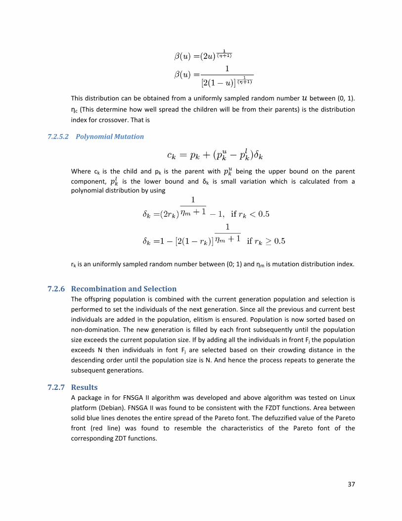
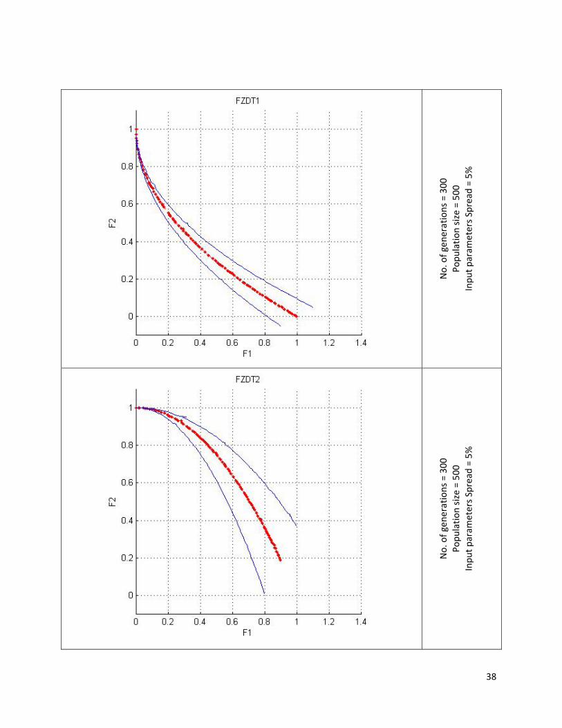
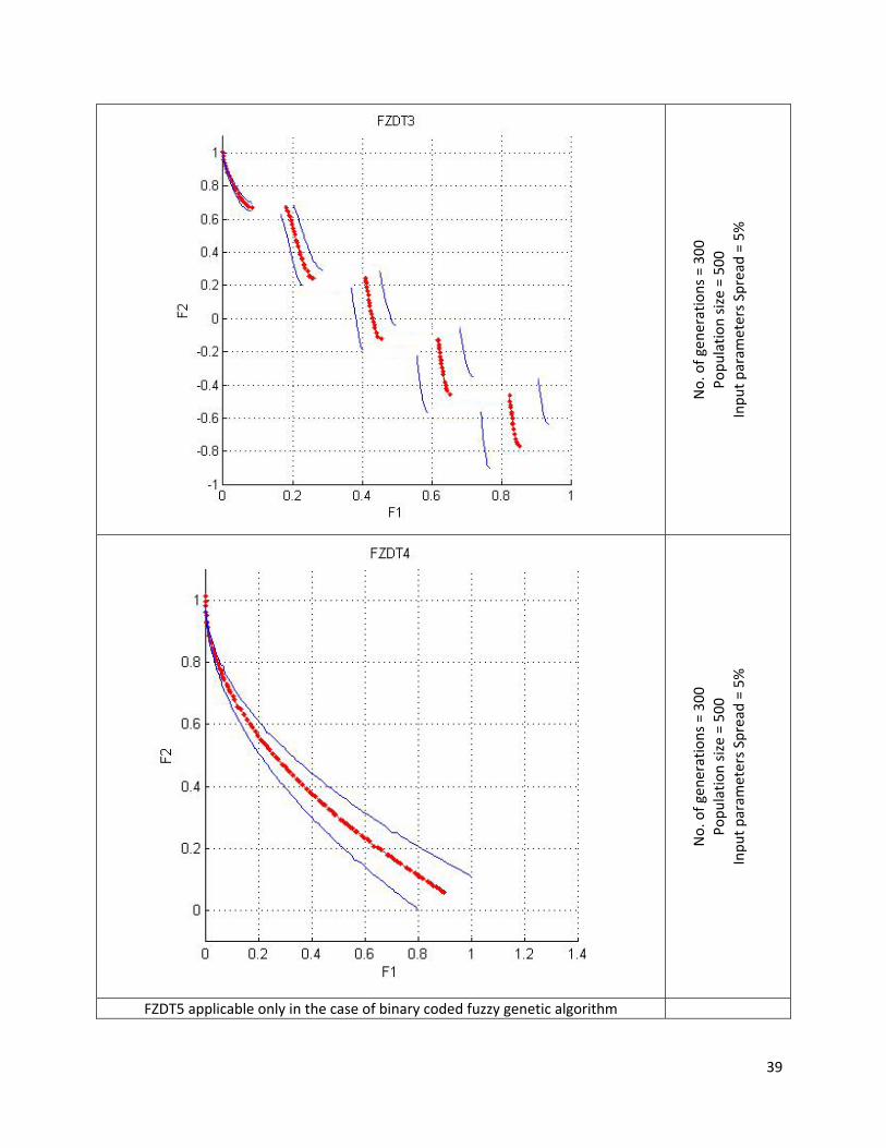
7.2.7 Results A package in for FNSGA II algorithm was developed and above algorithm was tested on Linux platform (Debian). FNSGA II was found to be consistent with the FZDT functions. Area between solid blue lines denotes the entire spread of the Pareto font. The defuzzified value of the Pareto front (red line) was found to resemble the characteristics of the Pareto font of the corresponding ZDT functions.

38

No. of gen

erations = 300

Po

pulatio

n size = 500

Inpu

t param

eters Spread

= 5%

No. of gen

erations = 300

Po

pulatio

n size = 500

Inpu

t param

eters Spread

= 5%

39

No. of gen

erations = 300

Po

pulatio

n size = 500

Inpu

t param

eters Spread

= 5%

No. of gen

erations = 300

Po

pulatio

n size = 500

Inpu

t param

eters Spread

= 5%

FZDT5 applicable only in the case of binary coded fuzzy genetic algorithm

40

No. of gen

erations = 300

Po

pulatio

n size = 500

Inpu

t param

eters Spread

= 5%

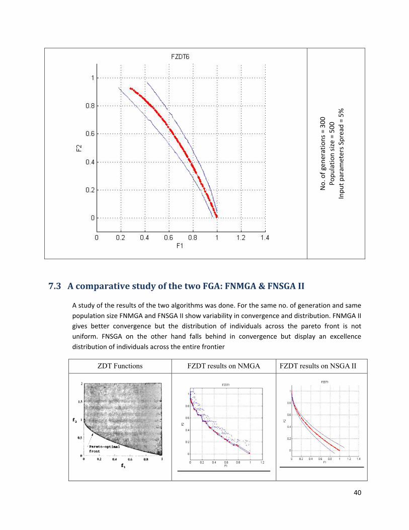
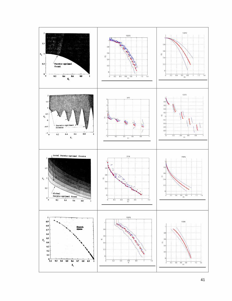
7.3 A comparative study of the two FGA: FNMGA & FNSGA II

A study of the results of the two algorithms was done. For the same no. of generation and same population size FNMGA and FNSGA II show variability in convergence and distribution. FNMGA II gives better convergence but the distribution of individuals across the pareto front is not uniform. FNSGA on the other hand falls behind in convergence but display an excellence distribution of individuals across the entire frontier

ZDT Functions FZDT results on NMGA FZDT results on NSGA II

42

8 Chapter 8 Conclusion

The FZDT results obtained from the two FGAs are in direct coherence with that of ZDT functions working in real environment. Fuzzy Genetic algorithm successfully maintained the shape and range of the frontier for all FZDT functions. The defuzzified values (GMI) of the elite members exactly copied the shape and range of the frontier for each of the ZDT functions for real environment. Therefore it can be concluded that the Fuzzy genetic algorithm very well captures the essence of multi objective optimization in fuzzy domain. And the proposed Fuzzy ZDT (FZDT) test functions can act as a benchmark for testing fuzzy genetic algorithms.

43

9 References

1) “Multi Objective Optimization using Evolutionary Algorithms” Kalyanmoy Deb, Wiley& sons Ltd.

2) S.H.Chen, C.H.Hsieh, Graded Mean Integration Representation of Generalized Fuzzy Numbers, Proceeding on Sixth Conference of Fuzzy Theory and its Applications (CD ROM), Chinese Fuzzy Systems Association, Taiwan, Republic of China (1998), 1‐6.

3) S.H.Chen, C.H.Hsieh, Ranking Generalized Fuzzy Numbers with Graded Mean Integration Representation, Proceeding of Eighth International Fuzzy Systems Association Word Congress (IFSA’99 Taiwan), Taiwan, Republic of China, 2(1999), 551‐555.

4) K.Deb, Multi‐objective Optimization using Evolutionary Algorithms, Wiley‐Interscience Series in Systems and Optimization, John Wiley & Sons, 2001.

5) Zitzler E., Deb k., Thiele L, (2000) Comparison of multi objective evolutionary algorithms: Empirical Results, Evolutionary computation journal 8(2), 125‐148.

6) H.J.Zimmermann, Fuzzy Set Theory and its Applications, Allied, Delhi & Kluwer, Boston, 1991. 7) D.Chakraborty, O.Dey, A Single‐Period Inventory Problem with Resalable Returns: A Fuzzy

Stochastic Approach, International Journal of Mathematical, Physical and Engineering Sciences, Volume 1, Number 1, 8‐15.

8) Jamison, K. D. and W. A. Lodwick, “Fuzzy linear programming using a penalty method”, Fuzzy sets and Systems, vol.119, pp.97‐110, 2001.

9) Wang, H. F. and M. L. Wang, “A Fuzzy Multi‐Objective Linear Programming”, Fuzzy sets and systems, Vol. 86, pp.61‐72, 1997.

10) Ching. J., “Fuzzy Linear model based on statistical confidence interval and interval‐valued”, Fuzzy set, European Journal of Operational research vol. 29, pp. 65‐86, 2001.

11) R A. Ribiro and F. M. Pires,”Fuzzy Linear Programming via Simulated Annealing”, Kybernetika, vol. 35, 1999, pp. 57‐67

12) Buckley, J.J.T. feuring and Y. Havashi ,”Neural net solutions to fuzzy linear programming”, Fuzzy sets and Systems, vol. 106, pp. 99‐111,1999.

13) Buckley, J.J. and T. Feuring, “Evolutionary algorithm solution to fuzzy problems: fuzzy linear programming”, Fuzzy sets and systems Vol.109, pp.35‐53, 2000.

14) A Fast and Elitist Multiobjective Genetic Algorithm: NSGA‐II, Kalyanmoy Deb, Amrit Pratap, Sameer Agarwal, and T. Meyarivan, IEEE TRANSACTIONS ON EVOLUTIONARY COMPUTATION, VOL. 6, NO. 2, APRIL 2002

15) Hans‐Georg Beyer and Kalyanmoy Deb. On Self‐Adaptive Features in Real‐Parameter Evolutionary Algorithm. IEEE Trabsactions on Evolutionary Computation, 5(3):250 ‐270, June 2001.

16) Kalyanmoy Deb and R. B. Agarwal. Simulated Binary Crossover for Continuous Search Space. Complex Systems, 9:115 ‐148, April 1995.

44

17) Kalyanmoy Deb, Amrit Pratap, Sameer Agarwal, and T. Meyarivan. A Fast Elitist Multi‐objective Genetic Algorithm: NSGA‐II. IEEE Transactions on Evolutionary Computation, 6(2):182‐ 197, April 2002.

18) M. M. Raghuwanshi and O. G. Kakde. Survey on multiobjective evolutionary and real coded genetic algorithms. In Proceedings of the 8th Asia Pacific Symposium on Intelligent and Evolutionasy Systems, pages 150 ‐ 161, 2004.

19) N. Srinivas and Kalyanmoy Deb. Multiobjective Optimization Using Nondominated Sorting in Genetic Algorithms. Evolutionary Computation, 2(3):221 ‐248, 1994.

20) K. Deb, 2001, Multiobjective Optimization using Evolutionary Algorithms, John‐Wiley, Chicheter.

21) C. A. Coello Coello, D. A. Van Veldhuizen and G. B. Lamont, 2002, Evolutionary Algorithms for Solving MultiObjective Poblems, Kluwer Academic Publishers, New York.

multi-objective fuzzy optimization & fuzzy zdt … · certificate this is to certify that the...

Documents