multi-fiber networks for video recognitionmulti-fiber networks 3 2 related work when it comes to...

Multi-Fiber Networks for Video Recognition

Yunpeng Chen1, Yannis Kalantidis2, Jianshu Li1,Shuicheng Yan3,1, and Jiashi Feng1

1 National University of Singapore2 Facebook Research

3 Qihoo 360 AI Institute{chenyunpeng, jianshu}@u.nus.edu, [email protected],

{eleyans, elefjia}@nus.edu.sg

Abstract. In this paper, we aim to reduce the computational cost ofspatio-temporal deep neural networks, making them run as fast as their2D counterparts while preserving state-of-the-art accuracy on video recog-nition benchmarks. To this end, we present the novel Multi-Fiber ar-chitecture that slices a complex neural network into an ensemble oflightweight networks or fibers that run through the network. To facil-itate information flow between fibers we further incorporate multiplexermodules and end up with an architecture that reduces the computationalcost of 3D networks by an order of magnitude, while increasing recogni-tion performance at the same time. Extensive experimental results showthat our multi-fiber architecture significantly boosts the efficiency of ex-isting convolution networks for both image and video recognition tasks,achieving state-of-the-art performance on UCF-101, HMDB-51 and Ki-netics datasets. Our proposed model requires over 9× and 13× less com-putations than the I3D [1] and R(2+1)D [2] models, respectively, yetproviding higher accuracy.

Keywords: Deep learning, neural networks, video, classification, actionrecognition

1 Introduction

With the aid of deep convolutional neural networks, image understanding hasachieved remarkable success in the past few years. Notable examples includeresidual networks [3] for image classification, FastRCNN [4] for object detection,and Deeplab [5] for semantic segmentation, to name a few. However, the progressof deep neural networks for video analysis still lags their image counterparts,mostly due to the extra computational cost and complexity of spatio-temporalinputs.

The temporal dimension of videos contains valuable motion information thatneeds to be incorporated for video recognition tasks. A popular and effectiveway of reasoning spatio-temporally is to use spatio-temporal or 3D convolu-tions [6,7] in deep neural network architectures to learn video representations.A 3D convolution is an extension of the 2D (spatial) convolution, which has

arX

iv:1

807.

1119

5v3

[cs

.CV

] 1

8 Se

p 20

18

2 Y. Chen, Y. Kalantidis, J. Li, S. Yan and J. Feng

three-dimensional kernels that also convolve along the temporal dimension. The3D convolution kernels can be used to build 3D CNNs (Convolutional NeuralNetworks) by simply replacing the 2D spatial convolution kernels. This keeps themodel end-to-end trainable. State-of-the-art video understanding models, suchas Res3D [7] and I3D [1] build their CNN models in this straightforward manner.They use multiple layers of 3D convolutions to learn robust video representationsand achieve top accuracy on multiple datasets, albeit with high computationaloverheads. Although recent approaches use decomposed 3D convolutions [2,8]or group convolutions [9] to reduce the computational cost, the use of spatio-temporal models still remains prohibitive for practical large-scale applications.For example, regular 2D CNNs require around 10s GFLOPs for processing asingle frame, while 3D CNNs currently require more than 100 GFLOPs for asingle clip4. We argue that a clip-based model should be able to highly outper-form frame-based models at video recognition tasks for the same computationalcost, given that it has the added capacity of reasoning spatio-temporally.

In this work, we aim to substantially improve the efficiency of 3D CNNs whilepreserving their state-of-the-art accuracy on video recognition tasks. Instead ofdecomposing the 3D convolution filters as in [2,8], we focus on the other sourceof computational overhead for 3D CNNs, the large input tensors. We proposea sparsely connected architecture, the Multi-Fiber network, where each unitin the architecture is essentially composed of multiple fibers, i.e. lightweight3D convolutional networks that are independent from each other as shown inFig 1(c). The overall network is thus sparsely connected and the computationalcost is reduced by approximately N times, where N is the number of fibersused. To improve information flow across fibers, we further propose a lightweightmultiplexer module, that redirects information between parallel fibers if neededand is attached at the head of each residual block. This way, with a minimalcomputational overhead, representations can be shared among multiple fibers,and the overall capacity of the model is increased.

Our main contributions can be summarized as follows:

1) We propose a highly efficient multi-fiber architecture, verify its effective-ness by evaluating it 2D convolutional neural networks for image recognitionand show that it can boost performance when embedded on common compactmodels.

2) We extend the proposed architecture to spatio-temporal convolutionalnetworks and propose the Multi-Fiber network (MF-Net) for learning robustvideo representations with significantly reduced computational cost, i.e. aboutan order of magnitude less than the current state-of-the-art 3D models.

3) We evaluate our multi-fiber network on multiple video recognition bench-marks and outperform recent related methods with several times lower compu-tational cost on the Kinetics, UCF-101 and HMDB51 datasets.

4 E.g. the popular ResNet-152 [3] and VGG-16 [10] models require 11 GFLOPs and15 GFLOPs, respectively, for processing a frame, while I3D [1] and R(2+1)D-34 [2]require 108 GFLOPs and 152 GFLOPs, respectively.

Multi-Fiber Networks 3

2 Related Work

When it comes to video models, the most successful approaches utilize deeplearning and can be split into two major categories: models based on spatial or2D convolutions and those that incorporate spatio-temporal or 3D convolutions.

The major advantage of adopting 2D CNN based methods is their compu-tational efficiency. One of the most successful approaches in this category isthe Two-stream Network [13] architecture. It is composed of two 2D CNNs, oneworking on frames and another on optical flow. Features from the two modalitiesare fused at the final stage and achieved high video recognition accuracy. Multipleapproaches have extended or incorporated the two-stream model [14,15,16,17]and since they are built on 2D CNNs are very efficient, usually requiring lessthan 10 GFLOPS per frame. In a very interesting recent approach, CoViAR [18]further reduces computations to 4.2 GFLOPs per frame in average, by directlyusing the motion information from compressed frames and sharing motion fea-tures across frames. However, as these approaches rely on pre-computed motionfeatures to capture temporal dependencies, they usually perform worse than 3Dconvolutional networks, especially when large video datasets are available forpre-training, such as Sports-1M [19] and Kinetics [20].

On the contrary, 3D convolution neural networks are naturally able to learnmotion features from raw video frames in an end-to-end manner. Since they use3D convolution kernels that model both spatial and temporal information, ratherthan 2D kernels which just model spatial information, more complex relationsbetween motion and appearance can be learned and captured. C3D [7] is oneof the early methods successfully applied to learning robust video features. Itbuilds a VGG [10] alike structure but uses 3 × 3 × 3 kernels to capture motioninformation. The Res3D [23] makes one step further by taking the advantageof residual connections to ease the learning process. Similarly, I3D [1] proposesto use the Inception Network [24] as the backbone network rather than residualnetworks to learn video representations. However, all of the methods suffer fromhigh computational cost compared with regular 2D CNNs due to the newlyadded temporal dimension. Recently, S3D [8] and R(2+1)D [2] are proposed touse one 1 × 3 × 3 convolution layer followed by another 3 × 1 × 1 convolutionallayer to approximate a full-rank 3D kernel to reduce the computations of a full-rank 3 × 3 × 3 convolutional layer while achieving better precision. However,these methods still suffer from an order of magnitude more computational costthan their 2D competitors, which makes it difficult to train and deploy them inpractical applications.

The idea of using spare connections to reduce the computational cost is sim-ilar to low-power networks built for mobile devices [25,26,27] as well as otherrecent approaches that try to sparsify parts of the network either through groupconvolutions [28] or through learning connectivity [29]. However, our proposednetwork is built for solving video recognition tasks and proposed different strate-gies that can also benefit existing low-power models, e.g. MobileNet-v2 [26]. Wefurther discuss the differences of our architecture and compare against the mostrelated and state-of-the-art methods in Sections 3 and 4.


3 × 3

3 × 3

3 × 3

3 × 3

3 × 3

3 × 3

Fiber 1 Fiber 2 Fiber 3 Fiber 1 Fiber 2 Fiber 3

Multiplexer

1 × 1

1 × 1

(a) (b) (c) (d)

3 × 3 Conv

3 × 3 Conv

Min

Mout

Mmid 3 × 3

3 × 3

3 × 3

3 × 3

3 × 3

3 × 3

Multiplexer

3 × 3 3 × 3 3 × 3

1 × 1

1 × 1

(e)

Fig. 1. From ResNet to multi-fiber. (a) A residual unit with two 3 × 3 convolutionlayers. (b) Conventional Multi-Path design, e.g. ResNeXt [28]. (c) The proposed multi-fiber design consisting of multiple separated lightweight residual units, called fibers. (d)The proposed multi-fiber architecture with a multiplexer for transferring informationacross separated fibers. (e) The architecture details of a multiplexer. It consists oftwo linear projection layers, one for dimension reduction and the other for dimensionexpansion.

3 Multi-Fiber Networks

The success of models that utilize spatio-temporal convolutions [7,1,2,8,9] sug-gests that it is crucial to have kernels spanning both the spatial and temporaldimensions. Spatio-temporal reasoning, however, comes at a cost: Both the con-volutional kernels and the input-output tensors are multiple times larger.

In this section, we start by describing the basic module of our proposedmodel, i.e., the multi-fiber unit. This unit can effectively reduce the number ofconnections within the network and enhance the model efficiency. It is genericand compatible with both 2D and 3D CNNs. For clearer illustration, we firstdemonstrate its effectiveness by embedding it into 2D convolutional architec-tures and evaluating its efficiency benefits for image recognition tasks. We thenintroduce its spatio-temporal 3D counterpart and discuss specific design choicesfor video recognition tasks.

3.1 The Multi-fiber Unit

The proposed multi-fiber unit is based on the highly modularized residual unit [3],which is easy to train and deploy. As shown in Figure 1(a), the conventional resid-ual unit uses two convolutional layers to learn features, which is straightforwardbut computationally expensive. To see this, let Min denote the number of in-put channels, Mmid denote the number of middle channels, and Mout denote thenumber of output channels. Then the total number of connections between thesetwo layers can be computed as

# Connections = Min ×Mmid + Mmid ×Mout. (1)


For simplicity, we ignore the dimensions of the input feature maps and convolu-tion kernels which are constant. Eqn. (1) indicates that the number of connec-tions is quadratic to the width of the network, thus increasing the width of theunit by a factor of k would result in k2 times more computational cost.

To reduce the number of connections that are essential to the overall com-putation cost, we propose to slice the complex residual unit into N paralleland separated paths (called fibers), each of which is isolated from the others,as shown in Figure 1(c). In this way, the overall width of the unit remains thesame, but the number of connections is reduced by a factor of N :

# Connections = N × (Min/N ×Mmid/N + Mmid/N ×Mout/N)

= (Min ×Mmid + Mmid ×Mout)/N. (2)

We set N = 16 for all our experiments, unless otherwise stated. As we show ex-perimentally in the following section, such a slicing strategy is intuitively simpleyet effective. At the same time, however, slicing isolates each path from the othersand blocks any information flow across them. This may result in limited learningcapacity for data representations since one path cannot access and utilize thefeature learned from the others. In order to recover part of the learning capacity,recent approaches that partially use slicing like ResNeXt [28], Xception [30] andMobileNet [25,26] choose to only slice a small portion of layers and still use fullyconnected parts. The majority of layers (> 60%) remains unsliced and domi-nates the computational cost, becoming the efficiency bottleneck. ResNeXt [28],for example, uses fully connected convolution layers at the beginning and endof each unit, and only slices the second layer as shown on Figure 1(b). However,these unsliced layers dominate the computation cost and become the bottleneck.Different from only slicing a small portion of layers, we propose to slice the entireresidual unit creating multiple fibers. To facilitate information flow, we furtherattach a lightweight bottleneck component we call the multiplexer that operatesacross fibers, in a residual manner.

The multiplexer acts as a router that redirects and amplifies features fromall fibers. As shown in Figure 1(e), the multiplexer first gathers features fromall fibers using a 1 × 1 convolution layer, and then redirects them to specificfibers using the following 1 × 1 convolution layer. The reason for using two1 × 1 layers instead of just one is to lower the computational overhead: weset the number of the first-layer output channels to be k times smaller thanits input channels, so that the total cost would be reduced by a factor of k/2compared with using a single 1×1 layer. The parameters within the multiplexerare randomly initialized and automatically adjusted by back-propagation end-to-end to maximize the performance gain for the given task. Batch normalizationand ReLU nonlinearities are used before each layer. Figure 1(d) shows the fullmulti-fiber network, where the proposed multiplexer is attached at the beginningof the multi-fiber unit for routing features extracted from other paralleled fibers.

We note that, although the proposed multi-fiber architecture is motivated toreduce the number of connections for 3D CNNs to alleviate high computationalcost, it is also applicable to 2D CNNs to further enhance efficiency of existing


2D architectures. To demonstrate this and verify effectiveness of the proposedarchitecture, we conduct several studies on 2D image classification tasks at first.

3.2 Justification of the Multi-fiber Architecture

We experimentally study the effectiveness of the proposed multi-fiber architec-ture by applying it on 2D CNNs for image classification and the ImageNet-1kdataset [31]. We use one of the most popular 2D CNN model, residual network(ResNet-18) [3], and the most computationally efficient ModelNet-v2 [26] as thebackbone CNN in the following studies.

Our implementation is based on the code released by [32] using MXNet [33]on a cluster of 32 GPUs. The initial learning rate is set to 0.5 and decreasesexponentially. We use a batch size of 1,024 and train the network for 360,000iterations. As suggested by prior work [25], we use less data augmentations forobtaining better results. Since the above training strategy is different from theone used in our baseline methods [3,26], we report both our reproduced resultsand the reported results in their papers for fair comparison.

2 2.5 3 3.5

Iterations 105

65

70

75

80

85

To

p-1

Acc

ura

cy

ResNet-18

ResNet-18 (MF embedded)

(a) ResNet-18

2 2.5 3 3.5

Iterations 105

60

65

70

75

To

p-1

Acc

ura

cy

MobileNet-v2

MobileNet-v2 (MF embedded)

(b) MobileNet-v2

Fig. 2. Training and validation accuracy on the ImagaNet-1k dataset for (a) ResNet-18and (b) MobileNet-v2 backbones respectively. The red lines stand for performance ofthe model with our proposed multi-fiber unit. The black lines show performance of ourreproduced baseline model using exactly the same training settings as our method. Theline thickness indicates results on the validation set (the ticker one) or the training set(the thinner one).

The training curves in Figure 2 plot the training and validation accuracy onImageNet-1k during the last several iterations. One can observe that the networkwith our proposed Multi-fiber (MF) unit can consistently achieve higher trainingand validation accuracy than the baseline models, with the same number of it-erations. Moreover, the resulted model has a smaller number of parameters andis more efficient (see Table 1). This demonstrates that embedding the proposedMF unit indeed helps reduce the model redundancy, accelerates the learning pro-cess and improves the overall model generalization ability. Considering the final


Table 1. Efficiency comparison on the ImageNet-1k validation set. “MF” stands for“multi-fiber unit”, and Top-1/Top-5 accuracies are evaluated on a 224 × 224 singlecenter crop [3]. “MF-Net” is our proposed network, with the architecture shown in2. The ResNeXt row presents results for a ResNeXt-26 model of our design that hasabout the same number of FLOPS as MF-Net.

Model Top-1 Acc. Top-5 Acc #Params FLOPs

ResNet-18 [3] 69.6 % 89.2 % 11.7 M 1.8 GResNet-18 (reproduced) 71.4 % 90.2 % 11.7 M 1.8 G

ResNet-18 (MF embedded) 74.3 % 92.1 % 9.6 M 1.6 G

ResNeXt-26 (8× 16d) 72.8 % 91.1 % 6.3 M 1.1 GResNet-50 [3] 75.3 % 92.2 % 25.5 M 4.1 G

MobileNet-v2 (1.4) [26] 74.7 % – 6.9 M 585 MMobileNet-v2 (1.4) (reproduced) 72.2 % 90.8 % 6.9 M 585 M

MobileNet-v2 (1.4) (MF embedded) 73.0 % 91.1 % 6.0 M 578 M

MF-Net (N = 12) 74.5 % 92.0 % 5.9 M 895 MMF-Net (N = 16) 74.6 % 92.0 % 5.8 M 861 MMF-Net (N = 24) 75.4 % 92.5 % 5.8 M 897 M

MF-Net (N = 16, w/o multiplexer) 70.2 % 89.4 % 4.5 M 600 MMF-Net (N = 16, w/o multiplexer, deeper & wider) 71.0 % 90.0 % 6.4 M 897 M

training accuracy of the “MF embedded” network is significantly higher thanthe baseline networks and all the network models adopt the same regularizationsettings, the MF units are also demonstrated to be able to improve the learningcapacity of the baseline networks.

Table 1 presents results on the validation set for Imagenet-1k. By simplyreplacing the original residual unit with our proposed multi-fiber one, we improvethe Top-1/Top-5 accuracy by 2.9%/1.9% upon ResNet-18 with smaller modelsize (9.6M vs. 11.7M ) and lower FLOPs (1.6G vs. 1.8G). The performancegain also stands for the more efficient low-complexity MobileNet-v2: introducingthe multi-fiber unit also boosts its Top-1/Top-5 accuracy by 0.8%/0.3% withsmaller model size (6.0M vs. 6.9M) and lower FLOPs (578M vs. 585M), clearlydemonstrating its effectiveness. We note that our reproduced MobileNet-v2 hasslightly lower accuracy than the reported one in [26] due to difference in thebatch size, learning rate and update policy. But with the same training strategy,our reproduced ResNet-18 is 1.8% better than the reported one [3].

The two bottom sections of Table 1 further show ablation studies of ourMF-Net, with respect to the number of fibers N and with/without the useof the multiplexer. As we see, increasing the number of fibers increases per-formance, while performance drops significantly when removing the multiplexerunit, demonstrating the importance of sharing information between fibers. Over-all, we see that our 2D multi-fiber network can perform as well as the much largerResNet-50 [3], that has 25.5M parameters and requires 4.1 GFLOPS5.

5 It is worth noting that in terms of wall-clock time measured on our server, our MF-Net is only slightly (about 30%) faster than the highly optimized implementationof ResNet-50. We attribute this to the unoptimized implementation of group convo-lutions in CuDNN and foresee faster actual running times in the near future whengroup convolution computations are well optimized.


(a) 3D Multi-fiber Network (b) 3D Multi-fiber Unit

Multiplexer

1 × 1× 1

1 × 1× 1

...

...

Previous Unit

3 × 3× 3

1 × 3× 3

Fiber 1

3 × 3× 3

1 × 3× 3

Fiber 2

3 × 3× 3

1 × 3× 3

Fiber N

...

Multiplexer

...

Next Unit

Video Conv 3×5×5stride (1,2,2)

Pool 1×3×3stride (1,2,2)

3D Multi-Fiber Unit

stride (2,1,1)

3D Multi-Fiber Unit

3D Multi-Fiber Unit

stride (1,2,2)

Global Pool(average)

3D Multi-Fiber Unit

3D Multi-Fiber Unit

stride (1,2,2)

3D Multi-Fiber Unit

3D Multi-Fiber Unit

FC Layer(classifier)

3D Multi-Fiber Unit

stride (1,2,2)

× 2

× 3× 5

× 2

Prediction

Fig. 3. Architecture of 3D multi-fiber network. (a) The overall architecture of 3D Multi-fiber Network. (b) The internal structure of each Multi-fiber Unit. Note that only thefirst 3 × 3 convolution layer has expanded on the 3rd temporal dimension for lowercomputational cost.

3.3 Spatio-temporal Multi-fiber Networks

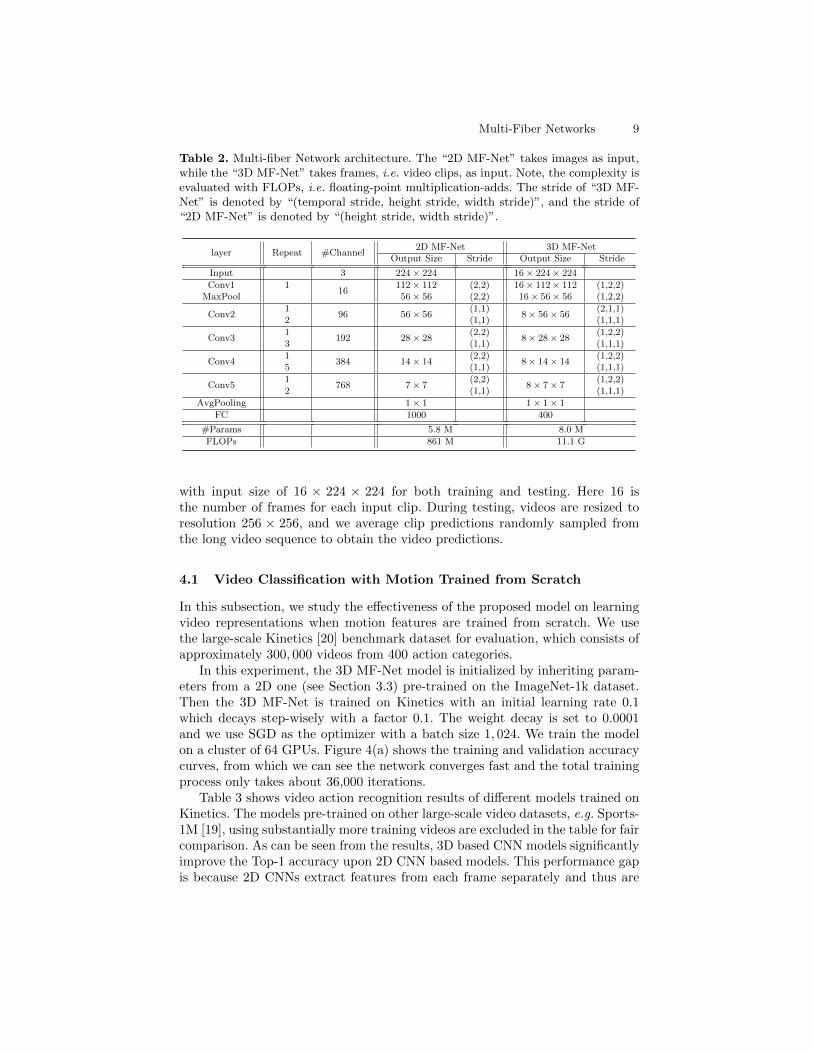
In this subsection, we extend out multi-fiber architecture to spatio-temporalinputs and present a new architecture for 3D convolutional networks and videorecognition tasks. The design of our spatio-temporal multi-fiber network followsthat of the “ResNet-34” [3] model, with a slightly different number of channelsfor lower GPU memory cost on processing videos. In particular, we reduce thenumber of channels in the first convolution layer, i.e. “Conv1”, and increase thenumber of channels in the following layers, i.e. “Conv2-5”, as shown in Table 2.This is because the feature maps in the first several layers have high resolutionsand consume exponentially more GPU memory than the following layers forboth training and testing.

The detailed network design is shown in Table 2, where we first design a 2DMF-Net and then “inflate” [1] its 2D convolutional kernels to 3D ones to buildthe 3D MF-Net. The 2D MF-Net is used as a pre-trained model for initializingthe 3D MF-Net. Several recent works advocate separable convolution which usestwo separate layers to replace one 3 × 3 layer [2,8]. Even though it may furtherreduce the computational cost and increase the accuracy, we do not use theseparable convolution due to its high GPU memory consumption, consideringvideo recognition application.

Figure 3 shows the inner structure of each 3D multi-fiber unit after the “infla-tion” from 2D to 3D. We note that all convolutional layers use 3D convolutionsthus the input and output features contain an additional temporal dimensionfor preserving motion information.

4 Experiments

We evaluate the proposed multi-fiber network on three benchmark datasets,Kinetics [20], UCF-101 [34] and HMDB51 [35], and compare the results withother state-of-the-art models. All experiments are conducted using PyTorch [36]


Table 2. Multi-fiber Network architecture. The “2D MF-Net” takes images as input,while the “3D MF-Net” takes frames, i.e. video clips, as input. Note, the complexity isevaluated with FLOPs, i.e. floating-point multiplication-adds. The stride of “3D MF-Net” is denoted by “(temporal stride, height stride, width stride)”, and the stride of“2D MF-Net” is denoted by “(height stride, width stride)”.

layer Repeat #Channel2D MF-Net 3D MF-Net

Output Size Stride Output Size Stride

Input 3 224× 224 16× 224× 224

Conv1 116

112× 112 (2,2) 16× 112× 112 (1,2,2)MaxPool 56× 56 (2,2) 16× 56× 56 (1,2,2)

Conv21

96 56× 56(1,1)

8× 56× 56(2,1,1)

2 (1,1) (1,1,1)

Conv31

192 28× 28(2,2)

8× 28× 28(1,2,2)

3 (1,1) (1,1,1)

Conv41

384 14× 14(2,2)

8× 14× 14(1,2,2)

5 (1,1) (1,1,1)

Conv51

768 7× 7(2,2)

8× 7× 7(1,2,2)

2 (1,1) (1,1,1)

AvgPooling 1× 1 1× 1× 1

FC 1000 400

#Params 5.8 M 8.0 M

FLOPs 861 M 11.1 G

with input size of 16 × 224 × 224 for both training and testing. Here 16 isthe number of frames for each input clip. During testing, videos are resized toresolution 256 × 256, and we average clip predictions randomly sampled fromthe long video sequence to obtain the video predictions.

4.1 Video Classification with Motion Trained from Scratch

In this subsection, we study the effectiveness of the proposed model on learningvideo representations when motion features are trained from scratch. We usethe large-scale Kinetics [20] benchmark dataset for evaluation, which consists ofapproximately 300, 000 videos from 400 action categories.

In this experiment, the 3D MF-Net model is initialized by inheriting param-eters from a 2D one (see Section 3.3) pre-trained on the ImageNet-1k dataset.Then the 3D MF-Net is trained on Kinetics with an initial learning rate 0.1which decays step-wisely with a factor 0.1. The weight decay is set to 0.0001and we use SGD as the optimizer with a batch size 1, 024. We train the modelon a cluster of 64 GPUs. Figure 4(a) shows the training and validation accuracycurves, from which we can see the network converges fast and the total trainingprocess only takes about 36,000 iterations.

Table 3 shows video action recognition results of different models trained onKinetics. The models pre-trained on other large-scale video datasets, e.g. Sports-1M [19], using substantially more training videos are excluded in the table for faircomparison. As can be seen from the results, 3D based CNN models significantlyimprove the Top-1 accuracy upon 2D CNN based models. This performance gapis because 2D CNNs extract features from each frame separately and thus are


0.5 1 1.5 2 2.5 3 3.5

Iterations 104

50

55

60

65

70

75

To

p-1

Cli

p A

ccu

racy

Training

Validation

(a)

101

102

FLOPs (x 109)

69

70

71

72

73

74

Vid

eo,

To

p-1

Acc

ura

cy (

%)

S3D

I3D-RGB

R(2+1)D-RGB

Ours

(b)

Fig. 4. Results on the Kinetics dataset (RGB Only). (a) The training and validationaccuracy for multi-fiber network. (b) Efficiency comparison between different 3D con-volutional networks. The area of each circle is proportional to the total parameternumber of the model.

Table 3. Comparison on action recognition accuracy with state-of-the-arts on Kinetics.The complexity is measured using FLOPs, i.e. floating-point multiplication-adds. Allresults are only using RGB information, i.e. no optical flow. Results with citationnumbers are copied from the respective papers.

Method #Params FLOPs Top-1 Top-5

Two-Stream [1] 12 M – 62.2 % –ConvNet+LSTM [1] 9 M – 63.3 % –

S3D [8] 8.8 M 66.4 G 69.4 % 89.1 %I3D-RGB [1] 12.1 M 107.9 G 71.1 % 89.3 %

R(2+1)D-RGB [2] 63.6 M 152.4 G 72.0 % 90.0 %

MF-Net (Ours) 8.0 M 11.1 G 72.8 % 90.4 %

incapable of modeling complex motion features from a sequence of raw frameseven when LSTM is used, which limits their performance. On the other hand, 3DCNNs can learn motion features end-to-end from raw frames and thus are ableto capture effective spatio-temporal information for video classification tasks.However, these 3D CNNs are computationally expensive compared 2D ones.

In contrast, our proposed MF-Net is more computationally efficient thanexisting 3D CNNs. Even with a moderate number of fibers, the computationaloverhead introduced by the temporal dimension is effectively compensated andour multi-fiber network only costs 11.1 GFLOPs, as low as regular 2D CNNs.Regarding performance and parameter efficiency, our proposed model achievesthe highest Top-1/Top-5 accuracy and meanwhile it has the smallest model size.Compared with the best R(2 + 1)D-RGB, our model is over 13× faster with8× less parameters, yet achieving 0.8% higher Top-1 accuracy. We note thatthe proposed model also costs the lowest GPU memory for both training andtesting, benefiting from the optimized architecture mentioned in Section 3.3.


Temporaldim

High

WidthInitialStates

FinalStates

RGB

Inputdim

Fig. 5. Visualization of the learned filters. The filters initialized by the ImageNet pre-trained model using inflating are shown on the top. The corresponding learned 3Dfilters on Kinetics are shown at the bottom. (upscaled by 15x). Best viewed in color.

To get further insights into what our network learns, we visualize all 16 spatio-temporal kernels of the first convolutional layer in Figure 5. Each 2-by-3 blockcorresponds to two 3×3×5×5 filters, with the top and bottom rows showing thefilter before and after learning, respectively. As the filters are initialized from a2D network pretrained on ImageNet and inflated in the temporal dimension, allthree sub-kernels are identical in the beginning. After learning, however, we seefilters evolving along the temporal dimension with diverse patterns, indicatingthat spatio-temporal features are learned effectively and embedded in these 3Dkernels.

4.2 Video Classification with Fine-tuned Models

In this experiment, we evaluate the generality and robustness of the proposedmulti-fiber network by transferring the features learned on Kinetics to otherdatasets. We are interested in examining whether the proposed model can learnrobust video representations that can generalize well to other datasets. We usethe popular UCF-101 [34] and HMDB51 [35] as evaluation benchmarks.

The UCF-101 contains 13, 320 videos from 101 categories and the HMDB51contains 6, 766 videos from 51 categories. Both are divided into 3 splits. Wefollow experiment settings in [7,23,2,8] and report the averaged three-fold crossvalidation accuracy. For model training on both datasets, we use an initial learn-ing rate 0.005 and decrease it for three times with a factor 0.1. The weight decayis set to 0.0001 and the momentum is set to 0.9 during the SGD optimization.All models are fine-tuned using 8 GPUs with a batch size of 128 clips.

Table 4 shows results of the multi-fiber network and comparison with state-of-the-art models. Consistent with above results, the multi-fiber network achievesthe state-of-the-art accuracy with much lower computation cost. In particular, onthe UCF-101 dataset, the proposed model achieves 96.0% Top-1 classification ac-curacy which is comparable with the sate-of-the-arts, but it is significantly morecomputationally efficient (11.1 vs. 152.4 GFLOPs). Compared with Res3D [23]which is also based on ResNet backbone and costs about 19.3 GFLOPs, themulti-fiber network achieves over 10% improvement in Top-1 accuracy (96.0%v.s. 85.8%) with 42% less computational cost.

Meanwhile, the proposed multi-fiber network also achieves the state-of-the-art accuracy on the HMDB51 dataset with significantly less computational cost.


Table 4. Action recognition accuracy on UCF-101 and HMDB51. The complexity isevaluated with FLOPs, i.e. floating-point multiplication-adds. The top part of the tablerefers to related methods based on 2D convolutions, while the lower part to methodsutilizing spatio-temporal convolutions. Column “+OF” denotes the use of Optical Flow.FLOPs for computing optical flow are not considered.

Method FLOPs +OF UCF-101 HMDB51

ResNet-50 [37] 3.8 G 82.3 % 48.9 %ResNet-152 [37] 11.3 G 83.4 % 46.7 %

CoViAR [18] 4.2 G 90.4 % 59.1 %Two-Stream [13] 3.3 G X 88.0 % 59.4 %

TSN [38] 3.8 G X 94.2 % 69.4 %

C3D [7] 38.5 G 82.3 % 51.6 %Res3D [23] 19.3 G 85.8 % 54.9 %

ARTNet [16] 25.7 G 94.3 % 70.9 %I3D-RGB [1] 107.9 G 95.6 % 74.8 %

R(2+1)D-RGB [2] 152.4 G 96.8 % 74.5 %

MF-Net (Ours) 11.1 G 96.0 % 74.6 %

101

102

FLOPs (x 109)

80

82

84

86

88

90

92

94

96

98

100

Vid

eo, T

op-1

Acc

ura

cy (

%)

C3D

Res3D

I3D-RGB

R(2+1)D-RGB

ARTNet

Ours

(a) UCF-101

101

102

FLOPs (x 109)

50

55

60

65

70

75

Vid

eo, T

op-1

Acc

ura

cy (

%)

C3D

Res3D

I3D-RGB

R(2+1)D-RGB

ARTNet

Ours

(b) HMDB51

Fig. 6. Efficiency comparison between different methods. We use the area of each circleto show the total number of parameters for each model.

Compared with the 2D CNN based models that also only use RGB frames, ourproposed model improves the accuracy by more than 15% (74.6% v.s. 59.1%).Even compared with the methods that using extra optical information, our pro-posed model still improves the accuracy by over 5%. This advantage partiallybenefits from richer motion features that learned from large-scale video pre-training datasets, while 2D CNNs cannot. Figure 6 shows the results in details.It is clear that our model provides an order of magnitude higher efficiency thanprevious state-of-the-arts in terms of FLOPs but still enjoys the high accuracy.

4.3 Discussion

The above experiments clearly demonstrate outstanding performance and effi-ciency of the proposed model. In this section, we discuss its potential limitationsthrough success and failure case analysis on Kinetics.


assembling computer 100% clapping 50% drinking shots 21%

surfing crowd 100% digging 50% fixing hair 20%

paragliding 98% kicking soccer ball 50% recording music 18%

playing chess 98% laughing 50% sneezing 18%

playing squash or racquetball 98% moving furniture 50% faceplanting 14%

presenting weather forecast 98% singing 50% headbutting 14%

sled dog racing 98% exercising arm 49% sniffing 10%

snowkiting 98% celebrating 48% slapping 4%

Fig. 7. Statistical results on Kinetics validation dataset. Left: Accuracy distributionof the proposed model on the validation set of Kinetics. The category is sorted byaccuracy in a descending order. Right: Selected categories and their accuracy.

We first study category-wise recognition accuracy. We calculate the accu-racy for each category and sort them in a descending order, shown in Figure7 (left). Among all 400 categories, we notice that 190 categories have an accu-racy higher than 80% and 349 categories have an accuracy higher than 50%.Only 17 categories cannot be recognized well and have an accuracy lower than30%. We list some examples along the spectrum in the right panel of Figure7. We find that in categories with highest accuracy there are either some spe-cific objects/backgrounds clearly distinguishable from other categories or specificactions spanning long duration. On the contrary, categories with low accuracyusually do not display any distinguishing object and the target action usuallylasts for a very short time within a long video.

To better understand success and failure cases, we visualize some of thevideo sequences in Figure 8. The frames are evenly selected from the long videosequence. As can be seen from the results, the algorithm is more likely to makemistakes on videos without any distinguishable object or containing an actionlasting a relatively short period of time.

5 Conclusion

In this work, we address the problem of building highly efficient 3D convolutionneural networks for video recognition tasks. We proposed a novel multi-fiberarchitecture, where sparse connections are introduced inside each residual blockeffectively reducing computations and a multiplexer is developed to compensatethe information loss. Benefiting from these two novel architecture designs, theproposed model greatly reduces both model redundancy and computational cost.Compared with existing state-of-the-art 3D CNNs that usually consume an orderof magnitude more computational resources than regular 2D CNNs, our proposedmodel costs significantly less resources yet achieves the state-of-the-art videorecognition accuracy on Kinetics, UCF-101, HMDB51. We also showed that theproposed multi-fiber architecture is a generic method which can also benefitexisting networks on image classification task.

Acknowledgements Jiashi Feng was partially supported by NUS IDS R-263-000-C67-646, ECRA R-263-000-C87-133 and MOE Tier-II R-263-000-D17-112.


drinking shots: 46.3% tasting beer: 14.5%

drinking: 12.7%drinking beer: 8.8%

tasting food: 4.9%

fixing hair: 86.0%curling hair: 3.9%

pumping fist: 1.0%singing: 1.0%

finger snapping: 0.8%

recording music: 96.4%drumming fingers: 1.3%

using remote controller (not gaming): 0.4%

playing bass guitar: 0.1%assembling computer: 0.1%

sneezing: 74.7%sticking tongue out: 11.0%

shaking head: 5.2%crying: 4.0%

laughing: 1.3%

faceplanting: 80.6%riding mountain bike: 5.0%

drop_kicking: 3.6%crossing_river: 2.2%

chopping_wood: 1.1%

headbutting: 63.3%shaking hands: 13.5%

slapping: 6.9%giving or receiving award: 2.1%

robot dancing: 1.9%

sniffing: 73.2%making jewelry: 4.3%

shuffling cards: 3.8%sharpening pencil: 2.7%

tapping pen: 2.5%

slapping: 15.4%dancing macarena: 10.0%

drop kicking: 5.1%finger snapping: 5.0%

rock scissors paper: 4.3%

cleaning gutters: 29.7%abseiling: 8.1%

watering plants: 7.4%cleaning windows: 6.4%

laying bricks: 5.3%

pushing wheelchair: 11.2%high kick: 9.2%

carrying baby: 8.1%tap dancing: 6.8%

country line dancing: 5.0%

playing saxophone: 90.7%playing clarinet: 9.3%

smoking hookah: 0.0%playing trumpet: 0.0%

playing trombone: 0.0%

eating cake: 69.0%eating ice cream: 9.5%

eating spaghetti: 9.3%reading book: 1.2%

blowing out candles: 1.2%

dancing ballet: 49.8%yoga: 11.4%

robot dancing: 4.0%trapezing: 3.6%

cheerleading: 2.7%

carrying baby: 89.6%hugging: 9.4%

crying: 0.1%waxing legs: 0.1%

cutting nails: 0.1%

picking fruit: 26.4%presenting weather forecast: 23.5%

planting trees: 9.5%snowboarding: 2.8%

watering plants: 2.7%

tasting beer: 17.4%eating burger: 10.6%

drinking: 10.2%drinking beer: 8.7%

blowing out candles: 8.5%

Fig. 8. Predictions made on the most difficult eight categories in Kinetics validationset. Left: Easy samples. Right: Hard samples. Top-5 confidence scores are shown beloweach video sequence. Underlines are used to emphasize correct prediction. Videos withinthe same row are from the same ground truth category.


References

1. Carreira, J., Zisserman, A.: Quo vadis, action recognition? a new model and thekinetics dataset. In: 2017 IEEE Conference on Computer Vision and PatternRecognition (CVPR), IEEE (2017) 4724–4733

2. Tran, D., Wang, H., Torresani, L., Ray, J., LeCun, Y., Paluri, M.: A closerlook at spatiotemporal convolutions for action recognition. arXiv preprintarXiv:1711.11248 (2017)

3. He, K., Zhang, X., Ren, S., Sun, J.: Deep residual learning for image recognition.In: Proceedings of the IEEE conference on computer vision and pattern recognition.(2016) 770–778

4. Girshick, R.: Fast r-cnn. arXiv preprint arXiv:1504.08083 (2015)

5. Chen, L.C., Papandreou, G., Kokkinos, I., Murphy, K., Yuille, A.L.: Deeplab:Semantic image segmentation with deep convolutional nets, atrous convolution,and fully connected crfs. arXiv preprint arXiv:1606.00915 (2016)

6. Karpathy, A., Toderici, G., Shetty, S., Leung, T., Sukthankar, R., Fei-Fei, L.: Large-scale video classification with convolutional neural networks. In: Proceedings of theIEEE conference on Computer Vision and Pattern Recognition. (2014) 1725–1732

7. Tran, D., Bourdev, L., Fergus, R., Torresani, L., Paluri, M.: Learning spatiotem-poral features with 3d convolutional networks. In: Computer Vision (ICCV), 2015IEEE International Conference on, IEEE (2015) 4489–4497

8. Xie, S., Sun, C., Huang, J., Tu, Z., Murphy, K.: Rethinking spatiotemporal featurelearning for video understanding. arXiv preprint arXiv:1712.04851 (2017)

9. Hara, K., Kataoka, H., Satoh, Y.: Can spatiotemporal 3d cnns retrace the historyof 2d cnns and imagenet. In: Proceedings of the IEEE Conference on ComputerVision and Pattern Recognition, Salt Lake City, UT, USA. (2018) 18–22

10. Simonyan, K., Zisserman, A.: Very deep convolutional networks for large-scaleimage recognition. arXiv preprint arXiv:1409.1556 (2014)

11. Shou, Z., Wang, D., Chang, S.F.: Temporal action localization in untrimmed videosvia multi-stage cnns. In: CVPR. (2016)

12. Shou, Z., Chan, J., Zareian, A., Miyazawa, K., Chang, S.F.: Cdc: Convolutional-de-convolutional networks for precise temporal action localization in untrimmedvideos. In: CVPR. (2017)

13. Simonyan, K., Zisserman, A.: Two-stream convolutional networks for action recog-nition in videos. In: Advances in neural information processing systems. (2014)568–576

14. Feichtenhofer, C., Pinz, A., Zisserman, A.: Convolutional two-stream networkfusion for video action recognition. IEEE Conference on Computer Vision andPattern Recognition (CVPR) (2016)

15. Ng, J.Y.H., Hausknecht, M., Vijayanarasimhan, S., Vinyals, O., Monga, R.,Toderici, G.: Beyond short snippets: Deep networks for video classification. In:Computer Vision and Pattern Recognition (CVPR), 2015 IEEE Conference on,IEEE (2015) 4694–4702

16. Wang, L., Li, W., Li, W., Van Gool, L.: Appearance-and-relation networks forvideo classification. arXiv preprint arXiv:1711.09125 (2017)

17. Tran, A., Cheong, L.F.: Two-stream flow-guided convolutional attention networksfor action recognition. International Conference on Computer Vision (2017)

18. Wu, C.Y., Zaheer, M., Hu, H., Manmatha, R., Smola, A.J., Krahenbuhl, P.: Com-pressed video action recognition. arXiv preprint arXiv:1712.00636 (2017)


19. Karpathy, A., Toderici, G., Shetty, S., Leung, T., Sukthankar, R., Fei-Fei, L.: Large-scale video classification with convolutional neural networks. In: CVPR. (2014)

20. Kay, W., Carreira, J., Simonyan, K., Zhang, B., Hillier, C., Vijayanarasimhan, S.,Viola, F., Green, T., Back, T., Natsev, P., et al.: The kinetics human action videodataset. arXiv preprint arXiv:1705.06950 (2017)

21. Shou, Z., Gao, H., Zhang, L., Miyazawa, K., Chang, S.F.: Autoloc: Weakly-supervised temporal action localization in untrimmed videos. In: ECCV. (2018)

22. Shou, Z., Pan, J., Chan, J., Miyazawa, K., Mansour, H., Vetro, A., Giro-i Nieto,X., Chang, S.F.: Online detection of action start in untrimmed, streaming videos.In: ECCV. (2018)

23. Tran, D., Ray, J., Shou, Z., Chang, S.F., Paluri, M.: Convnet architecture searchfor spatiotemporal feature learning. arXiv preprint arXiv:1708.05038 (2017)

24. Szegedy, C., Liu, W., Jia, Y., Sermanet, P., Reed, S., Anguelov, D., Erhan, D.,Vanhoucke, V., Rabinovich, A., et al.: Going deeper with convolutions

25. Howard, A.G., Zhu, M., Chen, B., Kalenichenko, D., Wang, W., Weyand, T., An-dreetto, M., Adam, H.: Mobilenets: Efficient convolutional neural networks formobile vision applications. arXiv preprint arXiv:1704.04861 (2017)

26. Sandler, M., Howard, A., Zhu, M., Zhmoginov, A., Chen, L.C.: Inverted residualsand linear bottlenecks: Mobile networks for classification, detection and segmenta-tion. arXiv preprint arXiv:1801.04381 (2018)

27. Zhang, X., Zhou, X., Lin, M., Sun, J.: Shufflenet: An extremely efficient convolu-tional neural network for mobile devices. arXiv preprint arXiv:1707.01083 (2017)

28. Xie, S., Girshick, R., Dollar, P., Tu, Z., He, K.: Aggregated residual transformationsfor deep neural networks. In: Computer Vision and Pattern Recognition (CVPR),2017 IEEE Conference on, IEEE (2017) 5987–5995

29. Ahmed, K., Torresani, L.: Maskconnect: Connectivity learning by gradient descent.In: European Conference on Computer Vision (ECCV). (2018)

30. Chollet, F.: Xception: Deep learning with depthwise separable convolutions. arXivpreprint (2017) 1610–02357

31. Krizhevsky, A., Sutskever, I., Hinton, G.E.: Imagenet classification with deep con-volutional neural networks. In: Advances in neural information processing systems.(2012) 1097–1105

32. Chen, Y., Li, J., Xiao, H., Jin, X., Yan, S., Feng, J.: Dual path networks. In:Advances in Neural Information Processing Systems. (2017) 4470–4478

33. Chen, T., Li, M., Li, Y., Lin, M., Wang, N., Wang, M., Xiao, T., Xu, B., Zhang,C., Zhang, Z.: Mxnet: A flexible and efficient machine learning library for hetero-geneous distributed systems. arXiv preprint arXiv:1512.01274 (2015)

34. Soomro, K., Zamir, A.R., Shah, M.: Ucf101: A dataset of 101 human actions classesfrom videos in the wild. arXiv preprint arXiv:1212.0402 (2012)

35. Kuehne, H., Jhuang, H., Garrote, E., Poggio, T., Serre, T.: Hmdb: a large videodatabase for human motion recognition. In: Computer Vision (ICCV), 2011 IEEEInternational Conference on, IEEE (2011) 2556–2563

36. Paszke, A., Gross, S., Chintala, S., Chanan, G.: Pytorch (2017)37. Feichtenhofer, C., Pinz, A., Wildes, R.P.: Spatiotemporal multiplier networks for

video action recognition. In: 2017 IEEE Conference on Computer Vision andPattern Recognition (CVPR), IEEE (2017) 7445–7454

38. Wang, L., Xiong, Y., Wang, Z., Qiao, Y., Lin, D., Tang, X., Van Gool, L.: Tem-poral segment networks: Towards good practices for deep action recognition. In:European Conference on Computer Vision, Springer (2016) 20–36

multi-fiber networks for video recognitionmulti-fiber networks 3 2 related work when it comes to...

Documents