multi-dimensional modeling of atmospheric copper...

SANDIA REPORT

SAND2004--5878 Unlimited Release Printed November 2004 Multi-dimensional Modeling of Atmospheric Copper-Sulfidation Corrosion on non-Planar Substrates

Ken S. Chen

Prepared by Sandia National Laboratories Albuquerque, New Mexico 87185 and Livermore, California 94550 Sandia is a multiprogram laboratory operated by Sandia Corporation, a Lockheed Martin Company, for the United States Department of Energys National Nuclear Security Administration under Contract DE-AC04-94AL85000. Approved for public release; further dissemination unlimited.

Issued by Sandia National Laboratories, operated for the United States Department of Energy by Sandia Corporation.

NOTICE: This report was prepared as an account of work sponsored by an agency of the United States Government. Neither the United States Government, nor any agency thereof, nor any of their employees, nor any of their contractors, subcontractors, or their employees, make any warranty, express or implied, or assume any legal liability or responsibility for the accuracy, completeness, or usefulness of any information, apparatus, product, or process disclosed, or represent that its use would not infringe privately owned rights. Reference herein to any specific commercial product, process, or service by trade name, trademark, manufacturer, or otherwise, does not necessarily constitute or imply its endorsement, recommendation, or favoring by the United States Government, any agency thereof, or any of their contractors or subcontractors. The views and opinions expressed herein do not necessarily state or reflect those of the United States Government, any agency thereof, or any of their contractors. Printed in the United States of America. This report has been reproduced directly from the best available copy. Available to DOE and DOE contractors from

U.S. Department of Energy Office of Scientific and Technical Information P.O. Box 62 Oak Ridge, TN 37831 Telephone: (865)576-8401 Facsimile: (865)576-5728 E-Mail: [email protected] Online ordering: http://www.osti.gov/bridge

Available to the public from

U.S. Department of Commerce National Technical Information Service 5285 Port Royal Rd Springfield, VA 22161 Telephone: (800)553-6847 Facsimile: (703)605-6900 E-Mail: [email protected] Online order: http://www.ntis.gov/help/ordermethods.asp?loc=7-4-0#online

2

3

SAND 2004-5878

Unlimited Release

Printed November 2004

Multi-dimensional Modeling of Atmospheric Copper-Sulfidation

Corrosion on non-Planar Substrates

Ken S. Chen

Multiphase Transport Processes Department

Sandia National Laboratories

P.O. Box 5800

Albuquerque, New Mexico 87185-0834

Abstract

This report documents the author’s efforts in the deterministic modeling of copper-

sulfidation corrosion on non-planar substrates such as diodes and electrical connectors. A

new framework based on Goma was developed for multi-dimensional modeling of

atmospheric copper-sulfidation corrosion on non-planar substrates. In this framework, the

moving sulfidation front is explicitly tracked by treating the finite-element mesh as a

pseudo solid with an arbitrary Lagrangian-Eulerian formulation and repeatedly performing

re-meshing using CUBIT and re-mapping using MAPVAR. Three one-dimensional studies

were performed for verifying the framework in asymptotic regimes. Limited model

validation was also carried out by comparing computed copper-sulfide thickness with

experimental data. The framework was first demonstrated in modeling one-dimensional

copper sulfidation with charge separation. It was found that both the thickness of the

space-charge layers and the electrical potential at the sulfidation surface decrease rapidly as

the Cu2S layer thickens initially but eventually reach equilibrium values as Cu2S layer

becomes sufficiently thick; it was also found that electroneutrality is a reasonable

approximation and that the electro-migration flux may be estimated by using the

equilibrium potential difference between the sulfidation and annihilation surfaces when the

Cu2S layer is sufficiently thick. The framework was then employed to model copper

sulfidation in the solid-state-diffusion controlled regime (i.e. stage II sulfidation) on a

prototypical diode until a continuous Cu2S film was formed on the diode surface. The

framework was also applied to model copper sulfidation on an intermittent electrical

contact between a gold-plated copper pin and gold-plated copper pad; the presence of Cu2S

was found to raise the effective electrical resistance drastically. Lastly, future research

needs in modeling atmospheric copper sulfidation are discussed.

4

Acknowledgment

This work was funded by the Accelerated Scientific Computing program and has benefited

from the numerous interactions within Sandia’s Corrosion Initiative spearheaded by Jeff

Braithwaite. In particular, the author would like to knowledge the helpful

interactions/discussions with Charles Barbour, Jeff Braithwaite, Michael Campin, David

Enos, Rich Larson, Harry Moffat, Rob Sorensen, and Amy Sun during the course of this

work. The author would also like to thank Harry Moffat and Amy Sun for careful reviews

of the manuscript and helpful comments.

5

Contents

1. Introduction 6

2. Simplified Physical Model 8

3. Kinetic Rates for the Sulfidation and Annihilation Reactions 9

4. Transport and Kinetic Time Constants 10

5. Governing Equations and Numerical Solution Methods 11

5.1 Species concentrations 11

5.2 Electric potential in copper sulfide with charge separation 12

5.3 Electric potential in one-dimensional sulfidation with

linear copper-vacancy and electron-hole concentrations 13

5.4 Mesh nodal displacement 14

5.5 Position of the sulfidation surface 15

5.6 Numerical solution methods, re-meshing and re-mapping 15

6. Computational Results and Discussion 16

6.1 Verification of Goma on solving the Poisson equation

that governs electric potential with charge separation 16

6.2 Verification of Goma for modeling transient diffusion processes

involving dilute solute species and slow surface chemical reaction 16

6.3 Verification of the Goma baseline model for atmospheric copper

sulfidation in the gas-phase-diffusion controlled regime with

fixed sulfidation-front approximation 17

6.4 Modeling one-dimensional copper sulfidation with charge separation 17

6.5 Modeling copper sulfidation on a prototypical diode 23

6.6 Modeling copper sulfidation on an intermittent electrical contact 29

7. Summary and Concluding Remarks 33

8. References 34

9. Appendices 37

Appendix A. On the Verification of Goma’s Capability for Modeling

Transient Diffusion Processes Involving Dilute Solute

Species and Slow Surface Chemical Reaction 37

Appendix B. On the Verification of Goma Baseline Model for Atmospheric

Copper Sulfidation in the Gas-phase-Diffusion Controlled

Regime – Fixed Sulfidation-Front Approximation 49

10. Distribution 61

6

1. Introduction

Copper-containing electrical and electronic devices (e.g., diodes, electrical interconnects)

can corrode to form corrosion products (e.g., copper sulfide) in the presence of a corroding

atmosphere containing hydrogen sulfide (H2S) and oxygen with some level of humidity

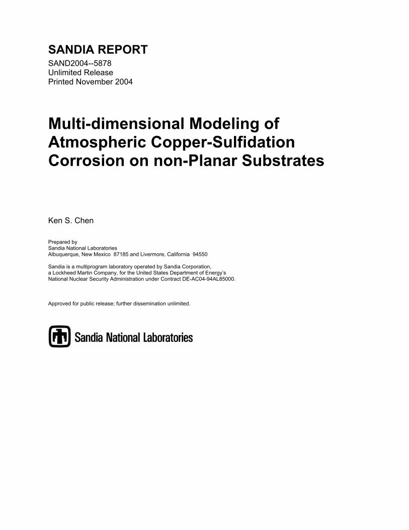
(see e.g., Sorensen et al. 1996, Sorensen et al. 2001, Braithwaite et al. 2003). Figure 1

shows examples of atmospheric corrosion observed in fielded copper-containing

components (Braithwaite et al. 2003, Moffat et al. 2000). Hydrogen sulfide is a product of

the anaerobic degradation of organic sulfur compounds (Leygraf and Graedel 2000); it may

also be generated from the decomposition of sulfur-containing parts (e.g., rubber seal rings)

nearby or surrounding the electrical and electronic devices. Formation of copper sulfide

(Cu2S) corrosion product, which occurs in a process called copper sulfidation, can have

detrimental effects or even cause malfunctions of copper-containing components. For

example, a continuous Cu2S film formed on the surface of a diode can conduct leakage

electrical current, which in turn can cause the diode to malfunction when the leakage

current is sufficiently high. Cu2S formed on an electrical contact can raise the effective

electrical resistance such that electrical current conducted through the contact under

constant voltage will be reduced to an unacceptably low level so as to render contact

failure. In short, understanding the mechanisms involved in copper-sulfidation corrosion

and being able to predict the rates of copper sulfidation for given environmental conditions

will be valuable in stockpile stewardship.

Due to its importance, atmospheric copper-sulfidation corrosion has attracted considerable

interests from inside and outside Sandia, and numerous studies have been carried out.

Graedel and his collaborators at AT&T (now Lucent Technologies) Bell Laboratories have

pioneered the studies of atmospheric copper sulfidation corrosion (see, e.g., Graedel et al.

1983, Graedel et al. 1985, Graedel et al. 1987, Graedel 1996, Tidblad and Graedel 1996) in

both experimental investigation and physical or mechanistic model development. The

textbook of Leygraf and Graedel (2000) summarizes the research work on atmospheric

copper-sulfidation corrosion conducted at the Royal Institute of Technology, Stockholm,

Sweden and at AT&T Bell Laboratories.

Atmospheric sulfidation of a diode has been first studied experimentally at Sandia by

Sorensen and Braithwaite and their collaborators (Sorensen et al. 1996, Krska et al. 1996).

An experimental study on the atmospheric degradation of gold- and nickel-gold-

electroplated copper connectors was carried out by Enos et al. (2003). The mechanisms of

atmospheric copper sulfidation were investigated by Barbour et al. (2002) using parallel

and conventional experimentation. The effect of gas-phase mass transport on atmospheric

copper sulfidation was studied by Braithwaite et al. (2000) whereas the effect of humidity

on atmospheric copper-sulfidation kinetics was examined by Enos et al. (2002). Studies on

the effects of varying humidity on copper sulfidation, in particular on the microstructure or

morphology of the Cu2S corrosion product, were carried out by Sullivan et al. (2004) and

Campin (2003). A long time (77 days) exposure test on the atmospheric corrosion of

copper by hydrogen sulfide in underground condition was conducted by Tran et al. (2003)

who show that exposure tests performed for short times in synthetic atmospheres cannot be

extrapolated to long time exposure in real conditions.

7

Figure 1. Examples of atmospheric corrosion observed in fielded copper-containing

components (Braithwaite et al. 2003, Moffat et al. 2000)

Larson (1998) made his first attempt at modeling the atmospheric sulfidation of copper by

proposing a physical copper-sulfidation model that includes four distinct phases: the

substrate metal, a cohensive cuprous sulfide (Cu2S) product layer, a thin aqueous film

adsorbed on the sulfide, and the ambient gas. Larson’s four-phase physical model is much

simpler than the six-regime GILDES model previously proposed by Graedel (1996), which

refers to Gas, the Interface between gas and liquid, the Liquid, the Deposition layer, the

Electrodic region near the surface (for conducting and semiconducting solids), and the

Solid. Larson further postulated that transport through the sulfide layer occurs via diffusion

and electromigration of copper vacancies and electron holes. Larson solved the pseudo-

steady state, one-dimensional governing equations (which describe the copper sulfidation

process based the physical model that he developed) numerically by employing the

standard SLATEC routine DNSQE and a shooting method coupled with DASSL (a stiff

ODE solver). Subsequently, Larson (2002) refined the copper-sulfidation model he

developed previously by focusing on the transport of charged lattice defects in a growing

Cu2S product layer between the ambient gas and the substrate metal. As previously, this

transport is postulated to occur via both diffusion and electromigration. Unlike the previous

model, however, the vacancy and hole annihilation reaction is taken to take place at the

copper/sulfide interface whereas the copper-sulfidation reaction is assumed to occur at the

sulfide/gas interface. Besides solving the governing equations in one-dimension

numerically as previously, Larson also obtained analytical solution for the asymptotic limit

Igniter Resistor

Diode

Rotary

Switch

Mosfet

Op Amp Chip carrier

Connector

8

of thick sulfide layer and found that the assumption of electroneutrality in the sulfide

(which can drastically simplify the numerical computations) gives rise to very little error

under typical conditions.

A multi-length-scale (from atomistic subgrid to multi-dimensional multi-phase continuum)

and multi-disciplinary approach was presented by Moffat et al. (2000) for modeling

atmospheric sulfidation of copper. Sandia’s efforts in developing an analytical capability

for predicting the effect of corrosion on the performance of electrical components were

reported by Sorensen et al. (2001) and Braithwaite et al. (2003). The efforts of multi-

dimensional modeling of atmospheric copper sulfidation on non-planar substrates such as

diodes and electrical connectors were presented by Chen (2003) and are documented in this

report. Portions of this report has been reported/documented in conference papers and

Sandia memoranda or reports (Chen 1999; Chen 2000a, 2000b; Sorensen et al. 2001; Chen

2002a, 2002b; Braithwaite et al. 2003; Chen 2003a, 2003b).

Other efforts, taken place or ongoing, include: 1) parameter estimation for an atmospheric

copper-sulfidation corrosion model by DAKOTA (Design Analysis Kit for Optimization

and Terascale Application), which was carried out by Sun and Moffat (2003); 2)

uncertainty quantification of an atmospheric corrosion model, which was performed by Sun

and Moffat (2004); and 3) model development for pore corrosion of noble-metal plated

electrical connectors, which were reported most recently by Moffat and Sun (2004a, 2004b

& 2004c).

2. Simplified Physical Model

In the present work, the essential phenomena involved in atmospheric copper sulfidation

were taken to occur according to the following simplified physical model (cf. Larson 2002,

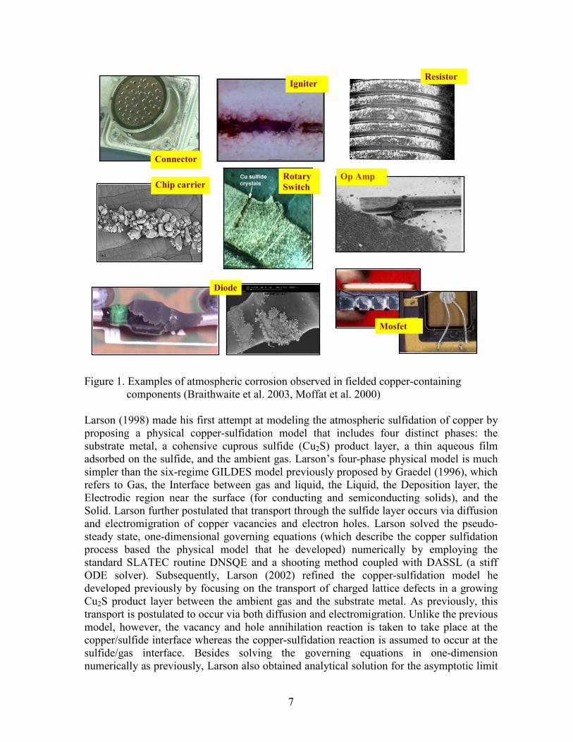
Chen 2002a & 2003b). As depicted in Figure 2, corrodant, H2S, diffuses from the

humidified atmosphere to the surface of the copper substrate initially and the Cu2S/air

interface subsequently. Simultaneously, copper vacancies and electron holes diffuse and

migrate within Cu2S from the stationary Cu/Cu2S interface to the moving Cu2S/air

interface. Copper vacancies (denoted as )−V and electron holes (denoted as )+h are

produced at the moving Cu2S/air interface via the following sulfidation electrochemical

reaction in which product water is taken to be liquid (cf. Larson 2002):

)(22)()(2

1)( 2222 lOHhVsSCugOgSH +++⇔+ +− (1)

where g, s, and l within the parentheses denotes gas, solid, and liquid, respectively. Once

reaching the Cu/Cu2S interface, copper vacancies and electron holes are annihilated as

follows (cf. Larson 2002):

NullhVCu →++ +− (2).

9

Figure 2. Schematic of a simplified physical model for atmospheric copper sulfidation

(not to scale).

Equation 1 represents an overall sulfidation reaction, which involves multiple steps as

follow: H2S gas dissolves into a bulk or thin water layer on the substrate surface, and then

dissociates partially as an acid. The process of S-2

undergoing oxidation occurs at a slow

rate; so slow that it is neglected here. The S-2

ions then react with the Cu2S surface to create

an extra lattice site. The reader is referred to Larson (1998)’s SAND report for a proposed

mechanism of the full process.

3. Kinetic Rates for the Sulfidation and Annihilation Reactions

Taking the forward and backward reactions in Equation 1 separately as elementary yields

the following kinetic rate expression (cf. Braithwaite 2002, Chen 2002a, Larson 2002,

Chen 2003b, Sun and Moffat 2003):

22

11

22

11 2222+−+− −− −=−=hVSHhVOSHSCu cckcKcckcckr (3)

where SCur 2 is the rate of formation of Cu2S; 1k and 1−k are the rate constants for,

respectively, the forward and backward reactions; SHc 2,

2Oc , −V

c and +hc are concentrations

of H2S, O2, −V (copper vacancy in the copper substrate) and +h (electron hole) species,

respectively; and 211 OckK = is a constant when both 1k and

2Oc are taken to be constant.

Note that concentrations of Cu2S and H2O do not appear in the rate expression in Equation

non-copper substrate

copper substrate

copper substrate



moving air/Cu2S interface

stationary Cu/Cu2S interface

H2S(g), air, H2O(g)

H2S(g), air, H2O(g)

H2S(g), air, H2O(g)

copper sulfide copper sulfide

copper sulfide

copper sulfide

copper substrate

H2S(g), air, H2O(g)

10

3 since Cu2S is produced as solid and H2O is taken to be produced as liquid so that their

concentrations are constant. Similarly, regarding the annihilation reaction (Equation 2) as

elementary yields (cf. Larson 2002, Chen 2003b):

+−=hVCu cckr 2 (4)

where Cur is the rate of consumption of copper. To account for the temperature effects on

the rate constants, k1, k-1 and k2, the Arrhenius expression can be used (Braithwaite 2002,

Chen 2003b):

RT

E

ekk1

11 '−

= (5),

RT

E

ekk1

11 '−−

−− = (6),

RT

E

ekk2

22 '−

= (7).

To capture effects of humidity, 1'k , 1'−k and 2'k can further be made functions of humidity.

4. Transport and Kinetic Time Constants

To have an appreciation on the relative time scales of the transport and kinetic processes

involved in atmospheric copper sulfidation occurring according to the simplified physical

model described above in section 2, it is helpful to estimate the process time constants. The

time constant for diffusion, τD, can be estimated via the following equation:

DLD /2=τ (8)

where L is some characteristic length scale and D is the diffusion coefficient. Since ionic

conductivity can be related to diffusivity via the Nernst-Eistein equation, time constant for

electro-migration can also be estimated by Equation 8. The time constant for the sulfidation

reaction can be estimated by

1/KLD =τ (9).

It is well known that the diffusivity for H2S diffusion in air, SHD 2, is about 0.1 cm

2/s.

Values for −VD (diffusivity of copper vacancies diffusion in Cu2S) and K1, however, are

not well known though Larson (2002) found that using −VD = 10

-10 cm

2/s and K1 = 1.21

cm/s yields good agreement between Sorensen and Braithwaite’s experimental data and his

11

model predictions. Separately, Moffat (2000) modeled the gas transport in a stagnation

point flow reactor that minimizes the gas phase mass transport resistance, and obtained a

sticking coefficient of 0.001 for H2S in Phase I growth of Cu2S, with a factor of 2 – 4

uncertainty. Using an effusive flux of 104

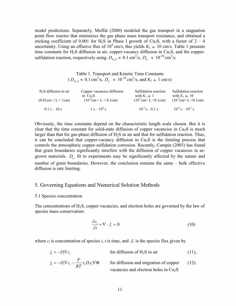
cm/s, this yields K1 ≈ 10 cm/s. Table 1 presents

time constants for H2S diffusion in air, copper-vacancy diffusion in Cu2S, and the copper-

sulfidation reaction, respectively using SHD 2≈ 0.1

cm

2/s, −VD ≈ 10

-10 cm

2/s.

Table 1. Transport and Kinetic Time Constants

( SHD 2≈ 0.1

cm

2/s, −VD ≈ 10

-10 cm

2/s, and K1 ≈ 1 cm/s)

H2S diffusion in air Copper vacancies diffusion Sulfidation reaction Sulfidation reaction

in Cu2S with K1 ≈ 1 with K1 ≈ 10

(0.01cm < L < 1cm) (10-5

cm < L < 0.1cm) (10-5

cm< L <0.1cm) (10-5

cm< L <0.1cm)

0.1 s – 10 s 1 s – 108 s 10

-5 s – 0.1 s 10

-6 s – 10

-2 s

Obviously, the time constants depend on the characteristic length scale chosen. But it is

clear that the time constant for solid-state diffusion of copper vacancies in Cu2S is much

larger than that for gas-phase diffusion of H2S in air and that for sulfidation reaction. Thus,

it can be concluded that copper-vacancy diffusion in Cu2S is the limiting process that

controls the atmospheric copper-sulfidation corrosion. Recently, Campin (2003) has found

that grain boundaries significantly interfere with the diffusion of copper vacancies in as-

grown materials. −VD fit to experiments may be significantly affected by the nature and

number of grain boundaries. However, the conclusion remains the same – bulk effective

diffusion is rate limiting.

5. Governing Equations and Numerical Solution Methods

5.1 Species concentration

The concentrations of H2S, copper vacancies, and electron holes are governed by the law of

species mass conservation:

0=⋅∇+∂

∂i

i Jt

c (10)

where ci is concentration of species i, t is time, and Ji is the species flux given by

iii cDj ∇−= for diffusion of H2S in air (11),

Φ∇−∇−= iiiiii cDzRT

FcDj for diffusion and migration of copper (12).

vacancies and electron holes in Cu2S

12

In Equations 11 and 12, Di and zi are, respectively, diffusivity and charge number of species i; F is Faraday’s constant (≡96487 C/mole) and R is the universal gas constant; and Φ is electric potential in Cu2S arising from the interactions between copper vacancies and electron holes.

5.2 Electric potential in copper sulfide with charge separation

The electric potential in Cu2S is governed by the law of charge conservation or the well-

known Poisson equation (cf. Newman 1991, Chen 2002):

)(2−+ −−=−=Φ∇ ∑ Vh

i

ii ccF

czF

εε (13)

where ε is permittivity of Cu2S in units of coulomb per volt per unit length (e.g., C/V-cm

or C/V-m). Since the electric filed, E, is defined as the negative of the electric potential,

i.e., Φ−∇=E , Equation 13 can be re-written in terms of electric fielc, E (cf. Larson 2002):

)( −+ −=∇Vhcc

FE

ε (14)

where electric field E has units of volts per unit length. Since the ratio 0/εε is called the

relative dielectric constant of a solid medium with 0ε being the permittivity of a vacuum

( ≡0ε 8.8542x10-14

C/V-cm), Equation 14 can be re-written as follows, using the relative

dielectric constant of the solid medium, :)/( 0εεκ ≡

)(0

−+ −=∇Vhcc

FE

κε (15).

It should be noted that Equation 15 differs from Larson (2002)’s Equation 6, which is due

to that 14 0 =πε in the cgs units (in which electric field has units of electric static unit per

cm) that Larson has chosen to write the Poisson equation; in contrast, electric field E in

Equation 15 has units of volts per unit length (e.g., V/cm or V/m). In short, Equation 15

above and Equation 6 in Larson (2002)’s paper are consistent but it should be kept in mind

that they are written with different units for the electric field. Substituting 0κεε = in

Equation 13 and re-arranging the resultant equation yields:

∑=

=−=Φ∇−⋅∇ −+

2

1

0 )()(i

iiVhczFccFκε (16),

13

which along with Equations 10 and 12 can be solved for Φ, −Vc , and +h

c . Equation 16

was incorporated in Goma by the author using the key word NET_CHARGE to specify

∑ iiczF as the current source and treating 0κε as the electrical conductivity.

In regions or domains in which +− =hVcc (i.e. electroneutrality constraint is met), Equation

16 reduces to the familiar Laplace equation:

02 =Φ∇ or )(tf=Φ∇ (17),

which means that the electric-potential gradient is a function of time only (that is, ∇Φ is

uniform spatially within the domain in which electroneutrality holds). A simple expression

for ∇Φ in 1-D approximation is the following:

hdy

d as Φ−Φ=

Φ=Φ∇ (18),

where y is the axis along with copper-vacancy and electron-hole transport; Φs and Φa are

electric potential at the sulfidation and annihilation surfaces, respectively; and h is the Cu2S

layer thickness.

5.3 Electric potential in one-dimensional sulfidation with linear copper-vacancy and

electron-hole concentrations

For the purpose of verifying Goma (a Sandia-developed finite-element computer code used

to solve the governing equations as discussed below in section 5.6) on solving the Poisson

equation that governs electric potential with charge separation, it is helpful to obtain an

analytical solution in some asymptotic regime. Equation 15 when written in one-

dimensional (along the Cu2S layer thickness direction or y-axis) becomes:

)(0

−+ −=Vhcc

F

dy

dE

κε (19).

We consider the an asymptotic regime in which the electron-hole and copper-vacancy

concentrations can be approximated as linear across the Cu2S layer and are given by,

respectively:

[ ] )0()0()()( ++++ +−=hhhhc

L

ycLcyc (20),

[ ] )0()0(2)0()()( −−++− +−+=VVhhVc

L

yccLcyc (21),

14

where L denotes thickness of the Cu2S layer; y = 0 refers to the annihilation surface (i.e.,

the Cu/Cu2S interface) and y = L the sulfidation surface. It can be readily shown from

Equations 20 and 21 that

)2/()2/( LcLcVh −+ = (22),

and

)0()0()()( −++− −=−VhhVccLcLc (23),

which are necessary conditions for satisfying the boundary conditions of vanishing electric

field at both the annihilation surface (y = 0) and the sulfidation surface (y = L):

E(0) = E(L) = 0. Substituting Equations 22 and 23 into Equation 19 and applying the

boundary condition of E(0) = 0 yields:

[ ] )()0()0()( 2

0

yLyccL

FyE

Vh−−= −+

κε (24).

Equation 24 clearly satisfies the boundary conditions of vanishing electric field at the

annihilation and sulfidation surfaces, i.e., E(0) = 0 and E(L) = 0. Substituting Φ−∇=E

into Equation 24 and solving for the electric potential Φ gives:

[ ] )3

1

2

1()0()0()0()( 32

0

yLyccL

Fy

Vh−−−=Φ−Φ −+

κε (25).

The electric potential gradient across the Cu2S layer in the asymptotic regime of linear

copper-vacancy and electron-hole concentrations can easily be determined from Eq. 25:

[ ])0()0(6

)0()(

0

−+ −−=Φ−Φ

Vhcc

FL

L

L

κε (26).

5.4 Mesh nodal displacement To solve for the nodal displacements of the finite-element mesh (the nodal positions of the mesh need to be solved for due to the moving sulfidation surface position being unknown apriori), we employed an arbitrary-Lagrangian-Eulerian formulation as developed by Sackinger et al. (1995) and treated the mesh as a pseudo solid that obeys the following equilibrium stress equation (Sackinger et al. 1995, and Schunk et al. 1997):

0=⋅∇ T (27)

where

IEET )(2 trmm λµ += (28)

and

15

[ ]T)()(2

1ddE ∇+∇= (29).

In the above equations d is the mesh displacement vector, I is the identity matrix, and µmJ

and λm are the Lame elastic coefficients, which are related to the familiar Young’s

modulus and Poisson ratio of the pseudo-solid mesh.

5.5 Position of the sulfidation surface

The position of the moving copper-sulfidation surface is determined by the local mass balance on Cu2S being formed at the sulfidation surface (i.e., the Cu2S/air interface):

SCu

SCu

SCu

ms rM

dt

dh2

2

2)(ρ

=−⋅= uun (30)

where h is the displacement or movement normal to the moving sulfidation surface

relative to a mesh (which is employed in obtaining the numerical solution to Equations 10,

11 or 12, and 16) moving with local velocity um, us is velocity of the sulfidation surface,

and n is unit vector normal to the sulfidation surface; SCu2ρ is density of Cu2S, SCuM

2 is the

molecular weight of Cu2S, and SCur 2is the molar rate of Cu2S formation as given by

Equation 3.

5.6 Numerical solution methods, re-meshing and re-mapping The governing equations 10, 11 or 12, and 16 are solved in GOMA, using i) finite-element

discretization with structured/unstructured meshes generated by CUBIT (a Sandia-

developed meshing tool, see http://endo.sandia.gov/cubit for details); ii) Galerkin weighted

residuals with quadratic basis function for species concentrations, electrolyte potential,

velocity, pressure, and nodal displacement unknowns; iii) a fully-coupled implicit solution

scheme via Newton’s method; adaptive time-step control (Adams-Bashforth predictor,

Moulton corrector); and parallel computing employing an iterative solver for the solution

of the resultant bAx = matrix-vector equations. Further details on the numerical solution

method can be found in the GOMA user’s guide (Schunk et al. 1997, Schunk et al. 2002).

Results presented in this report were all computed on a 48-processor network of 400 MHz

Sun Workstations using eight processors.

To handle the dramatic expansion in the Cu2S domain and to avoid mesh distortion, we

perform re-meshing every 10 – 20 time steps (depending on the substrate geometry,

process conditions, and the state of sulfidation) using CUBIT. Solution variables were

mapped from the old mesh to the new mesh using MAPVAR (a Sandia-developed utility

computer program, see Wellman 1999). We automated the process of re-meshing and re-

mapping using a Unix script. An example of re-meshing is presented in section 6.5.

16

6. Computational Results and Discussion

6.1 Verification of Goma on solving the Poisson equation that governs electric potential

with charge separation

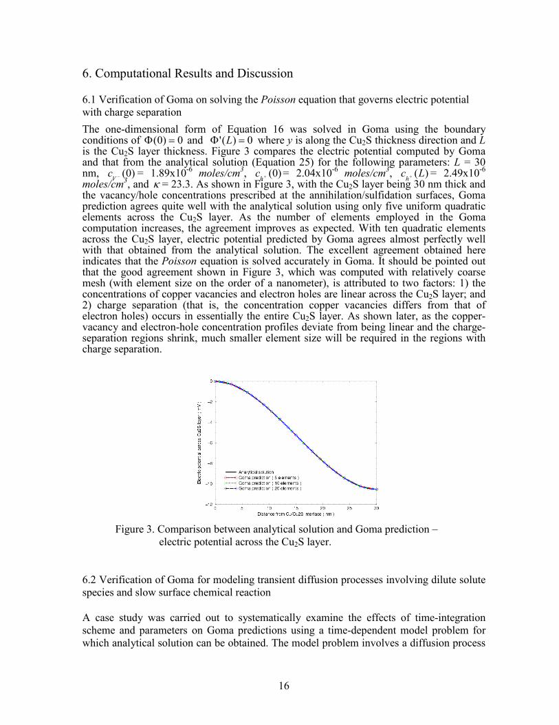
The one-dimensional form of Equation 16 was solved in Goma using the boundary conditions of 0)0( =Φ and 0)(' =Φ L where y is along the Cu2S thickness direction and L is the Cu2S layer thickness. Figure 3 compares the electric potential computed by Goma and that from the analytical solution (Equation 25) for the following parameters: L = 30 nm, )0(−V

c = 1.89x10-6 moles/cm

3, )0(+hc = 2.04x10

-6 moles/cm

3, )(Lc

h+ = 2.49x10-6

moles/cm3, and κ = 23.3. As shown in Figure 3, with the Cu2S layer being 30 nm thick and

the vacancy/hole concentrations prescribed at the annihilation/sulfidation surfaces, Goma prediction agrees quite well with the analytical solution using only five uniform quadratic elements across the Cu2S layer. As the number of elements employed in the Goma computation increases, the agreement improves as expected. With ten quadratic elements across the Cu2S layer, electric potential predicted by Goma agrees almost perfectly well with that obtained from the analytical solution. The excellent agreement obtained here indicates that the Poisson equation is solved accurately in Goma. It should be pointed out that the good agreement shown in Figure 3, which was computed with relatively coarse mesh (with element size on the order of a nanometer), is attributed to two factors: 1) the concentrations of copper vacancies and electron holes are linear across the Cu2S layer; and 2) charge separation (that is, the concentration copper vacancies differs from that of electron holes) occurs in essentially the entire Cu2S layer. As shown later, as the copper- vacancy and electron-hole concentration profiles deviate from being linear and the charge-separation regions shrink, much smaller element size will be required in the regions with charge separation.

Figure 3. Comparison between analytical solution and Goma prediction –

electric potential across the Cu2S layer.

6.2 Verification of Goma for modeling transient diffusion processes involving dilute solute

species and slow surface chemical reaction

A case study was carried out to systematically examine the effects of time-integration

scheme and parameters on Goma predictions using a time-dependent model problem for

which analytical solution can be obtained. The model problem involves a diffusion process

17

with a dilute solute species and a slow surface chemical reaction at one of the boundaries.

Details of this case study were communicated previously (Chen 2000a) and are presented

in Appendix A for convenience of reference. It was found that Goma predictions of solute-

species concentration profiles agree perfectly well with that given by the analytical solution

when proper time-integration scheme and parameters were employed. When inappropriate

time-integration scheme or parameters were used, however, significantly incorrect results

were obtained. As expected, the second-order accurate Crank-Nicholson time-integration

scheme yielded more accurate predictions as compared with the first-order accurate

backward-Euler method. Of the parameters used by Goma in time integration, the

maximum-time-step parameter was found to be most effective in reducing time-integration

errors. As a rule of thumb, the maximum time step allowed should be less than the time

constant of the process, based on the limited findings in the case study reported here.

Lastly, effect of mesh refinement was also examined and it was found that in modeling

transient processes errors resulted from inappropriate use of time integration scheme and

parameters are much more significant than that from the employment of an inadequately

refined mesh (that is, errors from time integration are much more pronounced than that

from mesh refinement).

6.3 Verification of the Goma baseline model for atmospheric copper sulfidation in the gas-

phase-diffusion controlled regime with fixed sulfidation-front approximation

A case study was conducted to verify the Goma baseline model for atmospheric copper

sulfidation in the gas-phase-diffusion controlled regime with the fixed sulfidation-front

approximation. Details of this case study were communicated previously (Chen 2000b) and

are presented in Appendix B for convenience of reference. Excellent agreement was found

between Goma predictions (H2S solute species concentration profiles and sulfide growth

layer thickness) and results from the analytical solution. Effects of maximum time step

allowed in Goma on H2S solute species concentration profiles and sulfide growth layer

thickness were examined and found to be significant (particularly when the maximum time

steps are large) – based on the case study carried out, it was found that a maximum time

step of 0.005 second yields nearly perfect agreement between Goma and analytical

predictions of sulfide layer thickness. The Goma model over-predicts the sulfide layer

thickness by about 3% with a maximum time step of 0.05 second, and by 18% with a

maximum time step of 0.5 second. After verification, the Goma model was employed to

study the effects of the boundary condition at the outer non-reacting surface on H2S solute

species concentration profiles and sulfide growth layer thickness. Lastly, to demonstrate its

utility, the Goma model was exercised to compute prediction of the average sulfide layer

thickness for a couple of hours of sulfidation using realistic transport/kinetic properties and

process conditions, and the boundary condition of constant H2S solute species

concentration on the outer non-reacting surface.

6.4 Modeling one-dimensional copper sulfidation with charge separation

When the substrate is planar, the copper sulfidation process can be taken as one

dimensional, i.e. along the thickness direction. In this section, numerical results of copper

sulfidation with charge separation computed in one-dimension are presented. Here,

18

Equations 10, 12, and 16 were solved in one dimension (along the thickness direction)

using Goma. The boundary conditions are as follow:

1) at the sulfidation surface, the normal component of the total fluxes of copper vacancies

and electron holes are set to equal to the rate of sulfidation given by Equation 3 with the

forward- and backward-reaction rate constants, k1 and k-1 given by Equations 5 and 6,

respectively.

2) at the annihilation surface, the normal component of the total fluxes of copper vacancies

and electron holes are set to equal to the rate of annihilation given by Equation 4 with the

rate constant, k2, given by Equation 7.

3) at both the sulfidation and annihilation surfaces, the electric-potential gradient is zero –

this is necessary in order to satisfy the zero-current (and zero-electric-field) condition there.

To accomplish this within Goma, the electric potential at the annihilation surface is set to

zero as a datum and the copper-vacancy concentration at the annihilation surface is iterated

until the zero current constraint is met – in the present work, this was done by employing

an augmenting condition in Goma.

4) Position of the moving sulfidation surface is given by Equation 30 and the internal mesh

nodal displacements are computed by solving Equations 27 – 29.

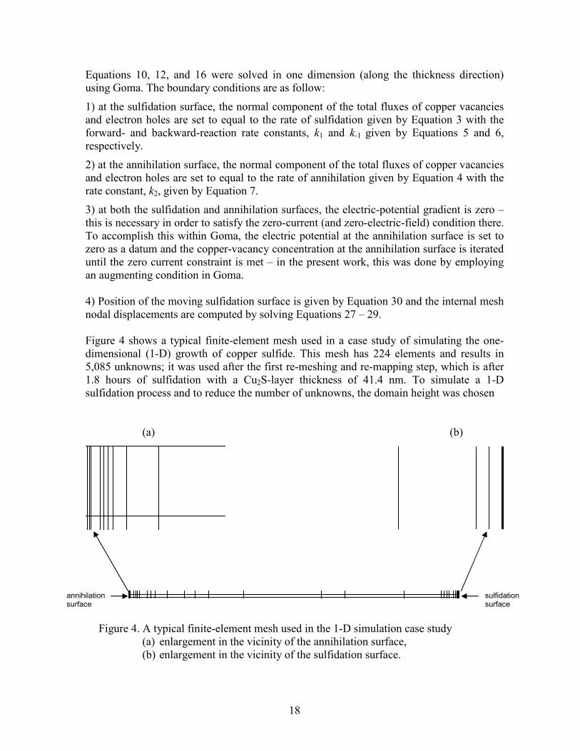
Figure 4 shows a typical finite-element mesh used in a case study of simulating the one-

dimensional (1-D) growth of copper sulfide. This mesh has 224 elements and results in

5,085 unknowns; it was used after the first re-meshing and re-mapping step, which is after

1.8 hours of sulfidation with a Cu2S-layer thickness of 41.4 nm. To simulate a 1-D

sulfidation process and to reduce the number of unknowns, the domain height was chosen

(a) (b)

Figure 4. A typical finite-element mesh used in the 1-D simulation case study

(a) enlargement in the vicinity of the annihilation surface,

(b) enlargement in the vicinity of the sulfidation surface.

annihilation surface

sulfidation surface

19

to be 3 nm and the smallest element size was fixed at 0.025 nm. As can be seen from

Figure 4 and its inserts, the elements are scaled toward the annihilation and sulfidation

surfaces where gradients exist. With the smallest element size being fixed at 0.025 nm, it is

easy to visualize that the number of unknowns grow rapidly as the Cu2S layer grows – this

increase is due to the number of columns of elements grow in order to maintain the

constant smallest element size (the number of rows of elements are held at four since the

Cu2S domain height is fixed at 3 nm).

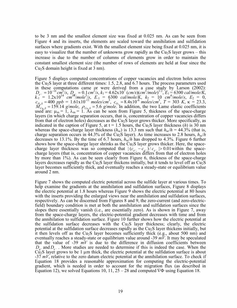
Figure 5 displays computed concentrations of copper vacancies and electron holes across the Cu2S layer at three different times: 1.5, 2.8, and 6.7 hours. The process parameters used in these computations came or were derived from a case study by Larson (2002):

1010−=−VD cm

2/s, 1.0=+hD cm

2/s, k1 = 4.62x10

7 (cm/s)(cm

3/mole)

1/2, E1 = 6300 cal/mole/K,

k-1 = 1.2x1014 cm

10/mole

3/s, E-1 = 6300 cal/mole/K, k2 = 10 cm

4/mole/s, E2 = 0,

=SHc 2400 ppb = 1.61x10

-11 moles/cm

3, =

2Oc 8.4x10

-6 moles/cm

3, T = 303 K, κ = 23.3,

=SCuM2

159.14 g/mole, =SCu2ρ 5.6 g/mole. In addition, the two Lame elastic coefficients

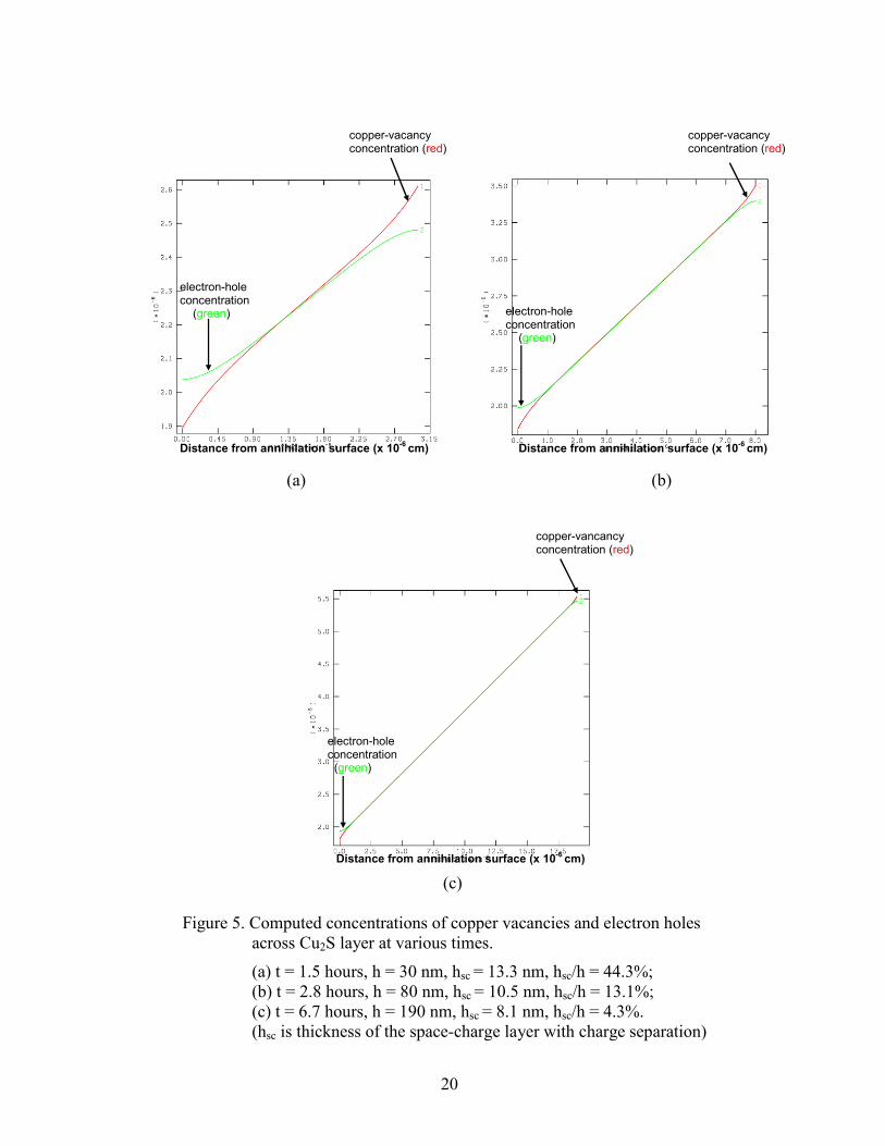
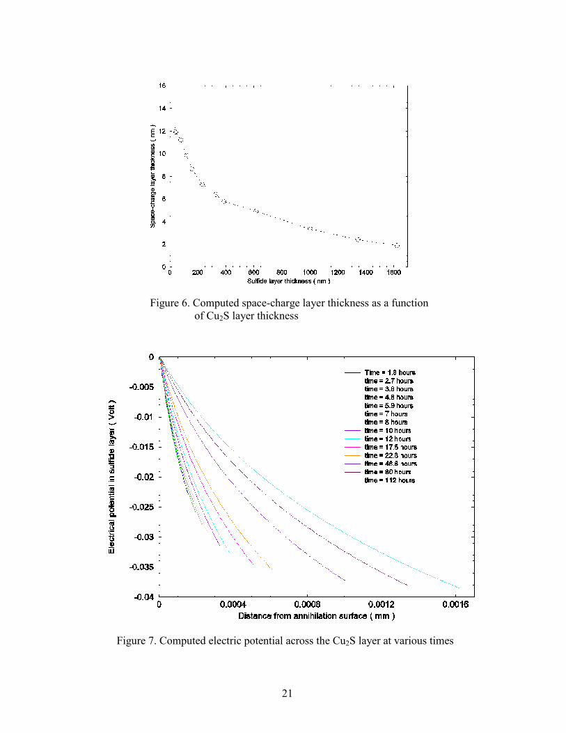
used are: µm = 1, λm = 1. As can be seen from Figure 5, thickness of the space-charge layers (in which charge separation occurs, that is, concentration of copper vacancies differs from that of electron holes) decreases as the Cu2S layer grows thicker. More specifically, as indicated in the caption of Figure 5, at t = 1.5 hours, the Cu2S layer thickness (h) is 30 nm whereas the space-charge layer thickness (hsc) is 13.3 nm such that hsc/h = 44.3% (that is, charge separation occurs in 44.3% of the Cu2S layer). As time increases to 2.8 hours, hsc/h decreases to 13.1%. By the time of 6.7 hours, hsc/h has dropped to 4.3%. Figure 6 further shows how the space-charge layer shrinks as the Cu2S layer grows thicker. Here, the space-charge layer thickness was so computed that 01.0|/)(| >− −+− VhV

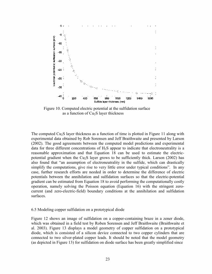
ccc within the space-charge layers (that is, concentration of copper vacancies differs from that of electron holes by more than 1%). As can be seen clearly from Figure 6, thickness of the space-charge layers decreases rapidly as the Cu2S layer thickens initially, but it tends to level off as Cu2S layer becomes sufficiently thick, and eventually reaches a steady-state or equilibrium value around 2 nm. Figure 7 shows the computed electric potential across the sulfide layer at various times. To help examine the gradients at the annihilation and sulfidation surfaces, Figure 8 displays the electric potential at 1.8 hours whereas Figure 9 shows the electric potential at 80 hours with the inserts providing the enlarged views near the annihilation and sulfidation surfaces, respectively. As can be discerned from Figures 8 and 9, the zero-current (and zero-electric- field) boundary condition is met at both the annihilation and sulfidation surfaces since the slopes there essentially vanish (i.e., are essentially zero). As is shown in Figure 7, away from the space-charge layers, the electric-potential gradient decreases with time and from the annihilation to sulfidation surface. Figure 10 further shows how the electric potential at the sulfidation surface decreases with the Cu2S layer thickness; clearly, the electric potential at the sulfidation surface decreases rapidly as the Cu2S layer thickens initially, but it then levels off as the Cu2S layer becomes sufficiently thick (e.g., about 500 nm) and eventually reaches a steady-state or equilibrium value around -39 mV. It may be speculated that the value of -39 mV is due to the difference in diffusion coefficients between

+hD and −V

D . More studies are needed to determine if this is indeed the case. When the Cu2S layer grows to be 1 µm thick, the electric potential at the sulfidation surface is about -37 mV, relative to the zero datum electric potential at the annihilation surface. To check if Equation 18 provides a reasonable approximation for computing the electric-potential gradient, which is needed in order to account for the migration flux (as described in Equation 12), we solved Equations 10, 11, 25 – 28 and computed ∇Φ using Equation 18.

(a) (b)

Figure 5. Computed

across Cu

(a) t = 1.5

(b) t = 2.8

(c) t = 6.7

(hsc is thic

Distance from annihilation surface (x 10-6

cm) Distance from annihilation surface (x 10-6

cm)

electron-hole concentration (green)

20

(c)

concentrations of copper vac

2S layer at various times.

hours, h = 30 nm, hsc = 13.3 n



kness of the space-charge lay

Distance from annihilation surface

copper-vancancy concentration (red)


ancies and electron ho

m, hsc/h = 44.3%;

m, hsc/h = 13.1%;

m, hsc/h = 4.3%.

er with charge separat

(x 10-6

cm)

copper-vacancy concentration (red)


copper-vacancy concentration (red)

les

ion)

21

Figure 6. Computed space-charge layer thickness as a function

of Cu2S layer thickness

Figure 7. Computed electric potential across the Cu2S layer at various times

22

Figure 8. Computed electric potential across the Cu2S layer at t = 1.8 hours

(a)

(b)

Figure 9. Computed electric potential across the Cu2S layer at t = 80 hours

(a) enlargement near annihilation surface;

(b) enlargement near sulfidation surface.

23

Figure 10. Computed electric potential at the sulfidation surface

as a function of Cu2S layer thickness

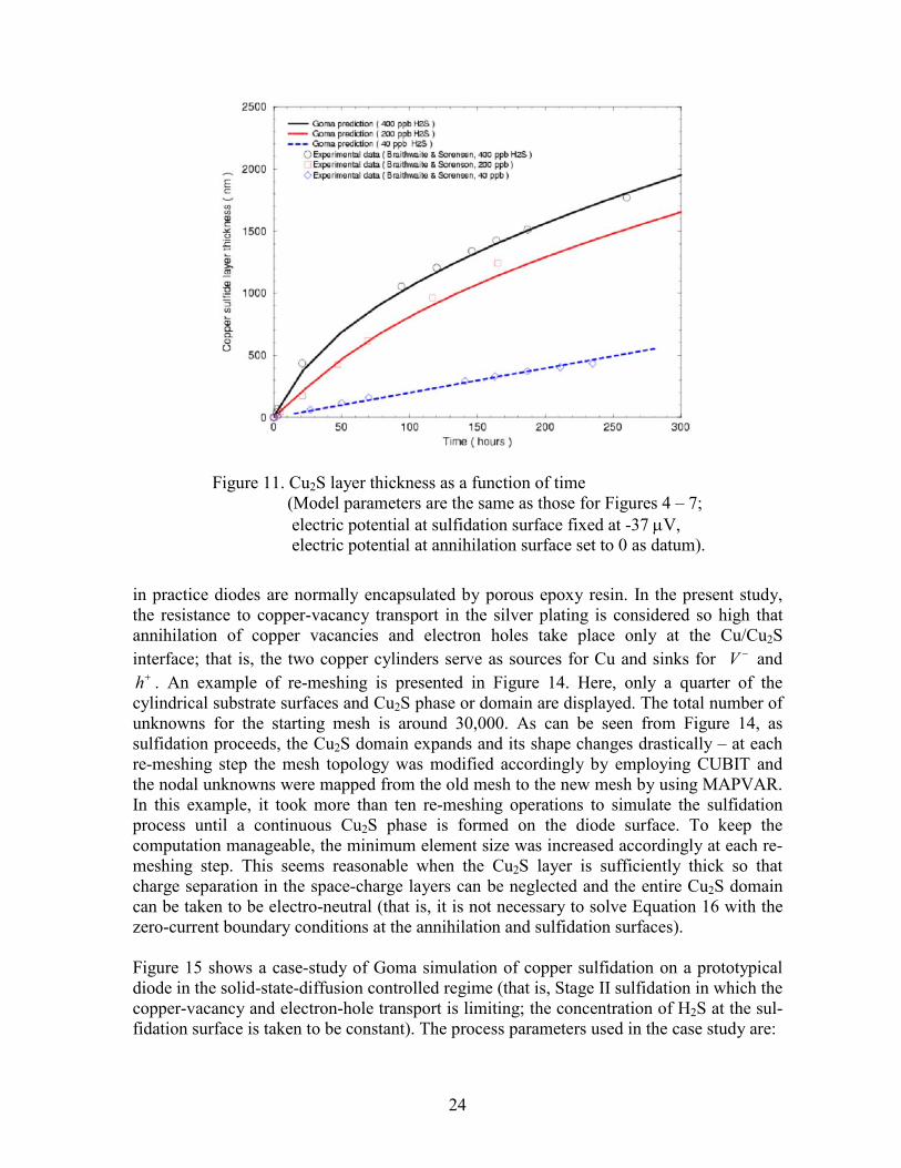
The computed Cu2S layer thickness as a function of time is plotted in Figure 11 along with

experimental data obtained by Rob Sorensen and Jeff Braithwaite and presented by Larson

(2002). The good agreements between the computed model predictions and experimental

data for three different concentrations of H2S appear to indicate that electroneutrality is a

reasonable approximation and that Equation 18 can be used to estimate the electric-

potential gradient when the Cu2S layer grows to be sufficiently thick. Larson (2002) has

also found that “an assumption of electroneutrality in the sulfide, which can drastically

simplify the computations, give rise to very little error under typical conditions”. In any

case, further research efforts are needed in order to determine the difference of electric

potentials between the annihilation and sulfidation surfaces so that the electric-potential

gradient can be estimated from Equation 18 to avoid performing the computationally costly

operation, namely solving the Poisson equation (Equation 16) with the stringent zero-

current (and zero-electric-field) boundary conditions at the annihilation and sulfidation

surfaces.

6.5 Modeling copper sulfidation on a prototypical diode

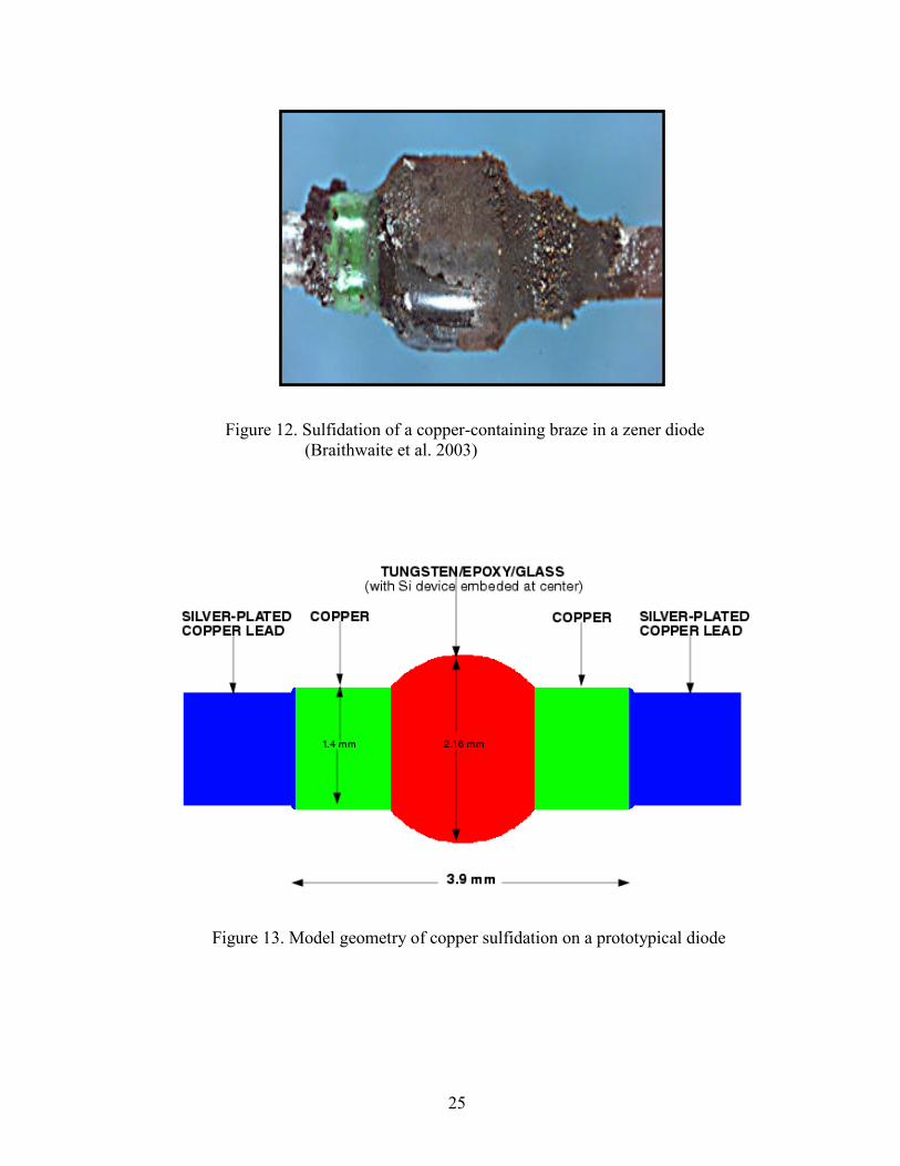
Figure 12 shows an image of sulfidation on a copper-containing braze in a zener diode,

which was obtained in a field test by Roben Sorensen and Jeff Braithwaite (Braithwaite et

al. 2003). Figure 13 displays a model geometry of copper sulfidation on a prototypical

diode, which is consisted of a silicon device connected to two copper cylinders that are

connected to two silver-plated copper leads. It should be noted that the model geometry

(as depicted in Figure 13) for sulfidation on diode surface has been greatly simplified since

24

Figure 11. Cu2S layer thickness as a function of time

(Model parameters are the same as those for Figures 4 – 7;

electric potential at sulfidation surface fixed at -37 µV,

electric potential at annihilation surface set to 0 as datum).

in practice diodes are normally encapsulated by porous epoxy resin. In the present study,

the resistance to copper-vacancy transport in the silver plating is considered so high that

annihilation of copper vacancies and electron holes take place only at the Cu/Cu2S

interface; that is, the two copper cylinders serve as sources for Cu and sinks for −V and +h . An example of re-meshing is presented in Figure 14. Here, only a quarter of the

cylindrical substrate surfaces and Cu2S phase or domain are displayed. The total number of

unknowns for the starting mesh is around 30,000. As can be seen from Figure 14, as

sulfidation proceeds, the Cu2S domain expands and its shape changes drastically – at each

re-meshing step the mesh topology was modified accordingly by employing CUBIT and

the nodal unknowns were mapped from the old mesh to the new mesh by using MAPVAR.

In this example, it took more than ten re-meshing operations to simulate the sulfidation

process until a continuous Cu2S phase is formed on the diode surface. To keep the

computation manageable, the minimum element size was increased accordingly at each re-

meshing step. This seems reasonable when the Cu2S layer is sufficiently thick so that

charge separation in the space-charge layers can be neglected and the entire Cu2S domain

can be taken to be electro-neutral (that is, it is not necessary to solve Equation 16 with the

zero-current boundary conditions at the annihilation and sulfidation surfaces).

Figure 15 shows a case-study of Goma simulation of copper sulfidation on a prototypical

diode in the solid-state-diffusion controlled regime (that is, Stage II sulfidation in which the

copper-vacancy and electron-hole transport is limiting; the concentration of H2S at the sul-

fidation surface is taken to be constant). The process parameters used in the case study are:

25

Figure 12. Sulfidation of a copper-containing braze in a zener diode

(Braithwaite et al. 2003)

Figure 13. Model geometry of copper sulfidation on a prototypical diode

26

(a) (b)

(d) (c)

Figure 14. An example of re-meshing in modeling copper sulfidation on a diode

(only a quarter of the substrate surface and Cu2S domain are displayed)

(a) starting mesh; (b) second re-meshing; (c) fourth re-meshing;

(d) nineth re-meshing.

(a) (b)

(d) (c)

Figure 15. Sample Goma predictions of copper sulfidation on a prototypical diode

in the solid-state-diffusion controlled regime (i.e. stage II sulfidation).

(a) time ~ 1 year; (b) time ~ 100 years; (c) time ~ 1500 years;

(d) time ~ 7000 years.

27

1010−=−VD cm

2/s, k1 = 1.46x10

7 (cm/s)(cm

3/mole)

1/2, E1 = 6300 cal/mole/K,

k-1 = 1.2x1014 cm

10/mole

3/s, E-1 = 6300 cal/mole/K, k2 = 10 cm

4/mole/s, E2 = 0, =SHc 2

400

ppm = 1.61x10-8 moles/cm

3, =

2Oc 8.4x10

-6 moles/cm

3, T = 303 K, =SCuM

2159.14 g/mole,

=SCu2ρ 5.6 g/mole, µm = 1, λm = 1, SiSCuc /, 2

θ = 60o ( SiSCuc /, 2

θ is angle of contact between

Cu2S and silicon-device surface), AgSCuc /, 2θ = 90

o ( AgSCuc /, 2θ is angle of contact between

Cu2S and silver-plating surface). In this case study, the Cu2S domain was taken to be

electro-neutral, that is, +− =hVcc , and the migration flux was neglected. With the diode

geometry as specified in Figure 13 and process parameters chosen as above, it takes ~ 7000

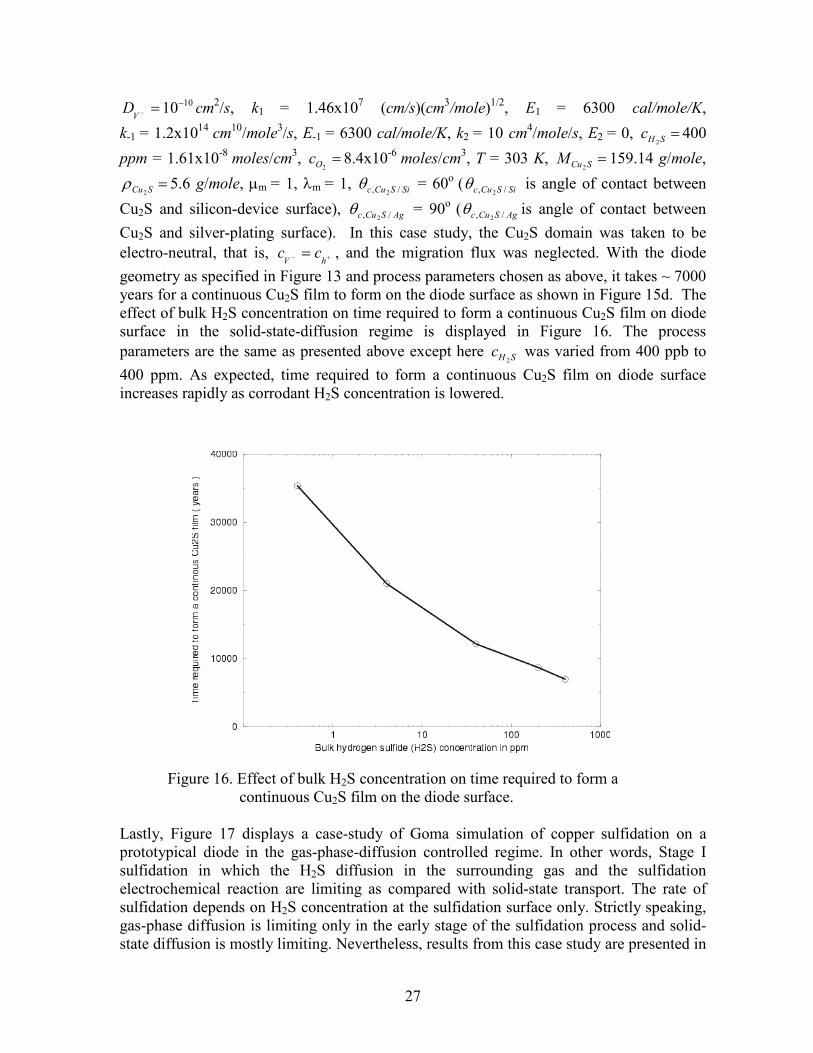
years for a continuous Cu2S film to form on the diode surface as shown in Figure 15d. The

effect of bulk H2S concentration on time required to form a continuous Cu2S film on diode

surface in the solid-state-diffusion regime is displayed in Figure 16. The process

parameters are the same as presented above except here SHc 2 was varied from 400 ppb to

400 ppm. As expected, time required to form a continuous Cu2S film on diode surface

increases rapidly as corrodant H2S concentration is lowered.

Figure 16. Effect of bulk H2S concentration on time required to form a

continuous Cu2S film on the diode surface.

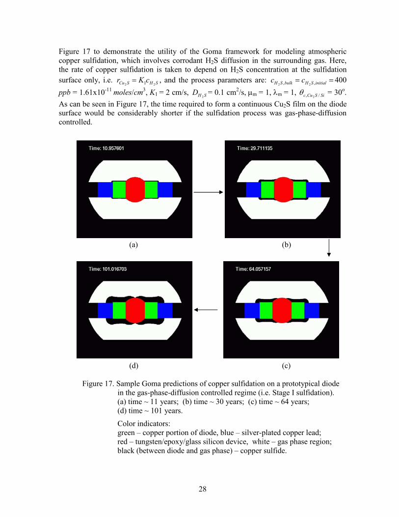
Lastly, Figure 17 displays a case-study of Goma simulation of copper sulfidation on a

prototypical diode in the gas-phase-diffusion controlled regime. In other words, Stage I

sulfidation in which the H2S diffusion in the surrounding gas and the sulfidation

electrochemical reaction are limiting as compared with solid-state transport. The rate of

sulfidation depends on H2S concentration at the sulfidation surface only. Strictly speaking,

gas-phase diffusion is limiting only in the early stage of the sulfidation process and solid-

state diffusion is mostly limiting. Nevertheless, results from this case study are presented in

28

Figure 17 to demonstrate the utility of the Goma framework for modeling atmospheric

copper sulfidation, which involves corrodant H2S diffusion in the surrounding gas. Here,

the rate of copper sulfidation is taken to depend on H2S concentration at the sulfidation

surface only, i.e. SHSCu cKr22 1= , and the process parameters are: == initialSHbulkSH cc ,, 22

400

ppb = 1.61x10-11 moles/cm

3, K1 = 2 cm/s, SHD 2

= 0.1 cm2/s, µm = 1, λm = 1, SiSCuc /, 2

θ = 30o.

As can be seen in Figure 17, the time required to form a continuous Cu2S film on the diode

surface would be considerably shorter if the sulfidation process was gas-phase-diffusion

controlled.

(a) (b)

(d) (c)

Figure 17. Sample Goma predictions of copper sulfidation on a prototypical diode

in the gas-phase-diffusion controlled regime (i.e. Stage I sulfidation).

(a) time ~ 11 years; (b) time ~ 30 years; (c) time ~ 64 years;

(d) time ~ 101 years.

Color indicators:

green – copper portion of diode, blue – silver-plated copper lead;

red – tungsten/epoxy/glass silicon device, white – gas phase region;

black (between diode and gas phase) – copper sulfide.

29

Copper contact pad

Gold-plated copper pin

~ 500 µm

6.6 Modeling copper sulfidation on an intermittent electrical contact

Figure 18 shows a schematic of copper-sulfidation corrosion on an electrical contact. Here,

a gold-plated copper pin (at top) is supposed to make good contact intermittently with a

gold-plated copper contact pad (at bottom). Now, suppose that a pinhole is present in the

gold plating (pinholes are present due to the imperfect plating process or impurity on

substrate surface) such that the copper pad is exposed to the surrounding gas polluted with

corrodant H2S for an extended time period in a relatively high-humidity, sulfidizing

environment. Consequently, copper sulfide will grow inside the pinhole and then outside it.

Figure 19 shows the simulated stage II copper sulfidation inside a pinhole with a diameter

Figure 18. Schematic of copper-sulfidation corrosion on electrical contact

(a)

(b)

(c)

Figure 19. Simulated growth of copper sulfide inside

(a) time ~ 1 hour; (b) time ~ 2 days; (c) t

copper sulfide

copper

gold

a pi

ime

Copper sulfide corrosion

product growing through

a pin hole in Au plating
Gold plating
nhole

~ 10 days.

30

of 25 µm and a height of 1.5 µm. The process parameters used in this case study are: 1010−=−V

D cm2/s, k1 = 4.62x10

7 (cm/s)(cm

3/mole)

1/2, E1 = 6300 cal/mole/K,

k-1 = 1.2x1014 cm

10/mole

3/s, E-1 = 6300 cal/mole/K, k2 = 10 cm

4/mole/s, E2 = 0,

=SHc 2400 ppb = 1.61x10

-11 moles/cm

3, =

2Oc 8.4x10

-6 moles/cm

3, T = 303 K,

=SCuM2

159.14 g/mole, =SCu2ρ 5.6 g/mole, µm = 1, λm = 1, AuSCuc /, 2

θ = 90o ( AuSCuc /, 2

θ is the

angle of contact between Cu2S and gold plating). In this case study, the migration flux has

been neglected. With the parameters specified and as can be seen from Figure 19, it takes

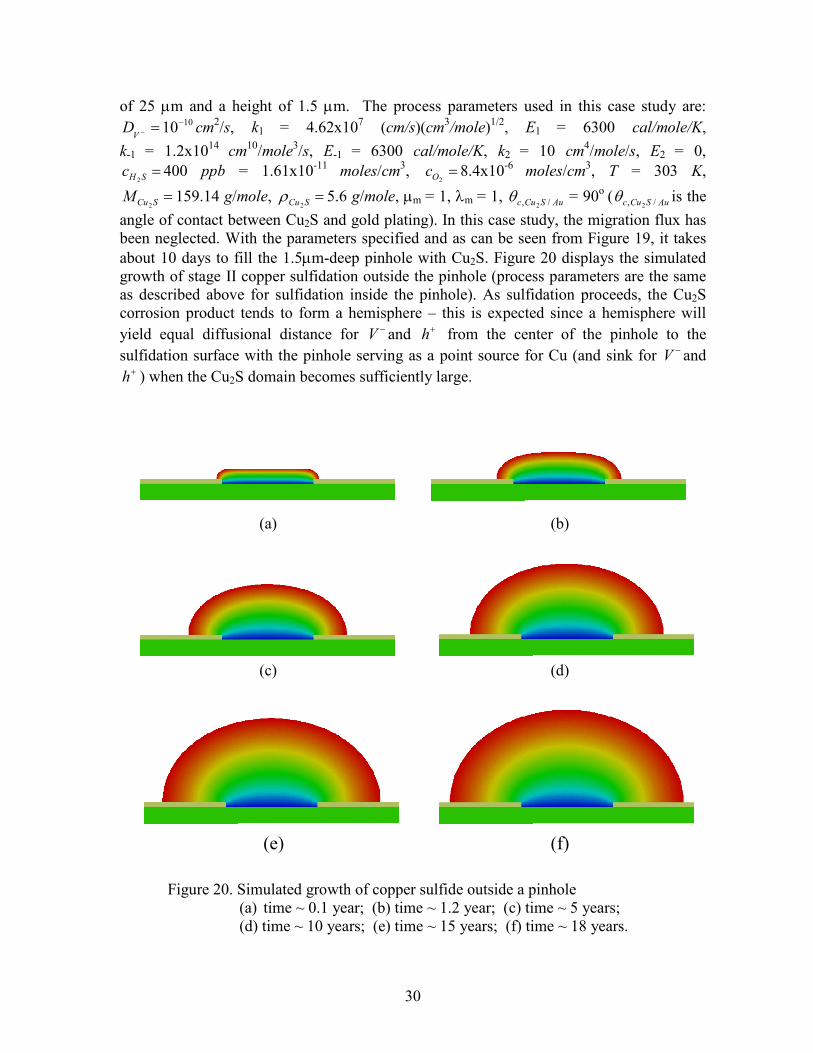
about 10 days to fill the 1.5µm-deep pinhole with Cu2S. Figure 20 displays the simulated

growth of stage II copper sulfidation outside the pinhole (process parameters are the same

as described above for sulfidation inside the pinhole). As sulfidation proceeds, the Cu2S

corrosion product tends to form a hemisphere – this is expected since a hemisphere will

yield equal diffusional distance for −V and +h from the center of the pinhole to the

sulfidation surface with the pinhole serving as a point source for Cu (and sink for −V and +h ) when the Cu2S domain becomes sufficiently large.

(a) (b)

(c) (d)

(e) (f)

Figure 20. Simulated growth of copper sulfide outside a pinhole

(a) time ~ 0.1 year; (b) time ~ 1.2 year; (c) time ~ 5 years;

(d) time ~ 10 years; (e) time ~ 15 years; (f) time ~ 18 years.

31

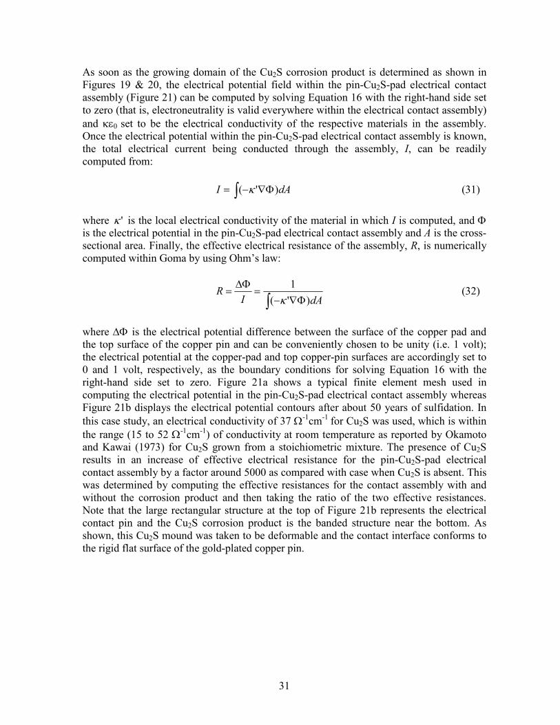
As soon as the growing domain of the Cu2S corrosion product is determined as shown in

Figures 19 & 20, the electrical potential field within the pin-Cu2S-pad electrical contact

assembly (Figure 21) can be computed by solving Equation 16 with the right-hand side set

to zero (that is, electroneutrality is valid everywhere within the electrical contact assembly)

and κε0 set to be the electrical conductivity of the respective materials in the assembly.

Once the electrical potential within the pin-Cu2S-pad electrical contact assembly is known,

the total electrical current being conducted through the assembly, I, can be readily

computed from:

∫ Φ∇−= dAI )'( κ (31)

where 'κ is the local electrical conductivity of the material in which I is computed, and Φ

is the electrical potential in the pin-Cu2S-pad electrical contact assembly and A is the cross-

sectional area. Finally, the effective electrical resistance of the assembly, R, is numerically

computed within Goma by using Ohm’s law:

∫ Φ∇−=

ΔΦ=

dAIR

)'(

1

κ (32)

where ΔΦ is the electrical potential difference between the surface of the copper pad and

the top surface of the copper pin and can be conveniently chosen to be unity (i.e. 1 volt);

the electrical potential at the copper-pad and top copper-pin surfaces are accordingly set to

0 and 1 volt, respectively, as the boundary conditions for solving Equation 16 with the

right-hand side set to zero. Figure 21a shows a typical finite element mesh used in

computing the electrical potential in the pin-Cu2S-pad electrical contact assembly whereas

Figure 21b displays the electrical potential contours after about 50 years of sulfidation. In

this case study, an electrical conductivity of 37 Ω-1

cm-1

for Cu2S was used, which is within

the range (15 to 52 Ω-1

cm-1

) of conductivity at room temperature as reported by Okamoto

and Kawai (1973) for Cu2S grown from a stoichiometric mixture. The presence of Cu2S

results in an increase of effective electrical resistance for the pin-Cu2S-pad electrical

contact assembly by a factor around 5000 as compared with case when Cu2S is absent. This

was determined by computing the effective resistances for the contact assembly with and

without the corrosion product and then taking the ratio of the two effective resistances.

Note that the large rectangular structure at the top of Figure 21b represents the electrical

contact pin and the Cu2S corrosion product is the banded structure near the bottom. As

shown, this Cu2S mound was taken to be deformable and the contact interface conforms to

the rigid flat surface of the gold-plated copper pin.

(a)

Figure 21. Pin-Cu2S

(a) finite

(b) elect

500 µm

32

(b)

-pad electrical contact assembly

element mesh;

rical potential contours at t ~ 50 ye

300 µm

ars.

Cu2S

Gold-plated

copper pin

gold-plated copper pad

33

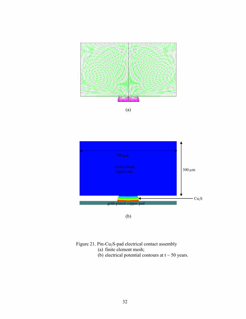
7. Summary and Concluding Remarks

A new framework based on Goma was developed and demonstrated for multi-dimensional

modeling of atmospheric copper-sulfidation corrosion on non-planar substrates such as

diodes and electrical contacts. In this framework, the moving sulfidation front is explicitly

tracked by treating the finite-element mesh as a pseudo solid with an arbitrary Lagrangian-

Eulerian formulation and repeatedly performing re-meshing using CUBIT and re-mapping

using MAPVAR. To gain confidence on the framework, three one-dimensional Goma-

verification studies were carried out: 1) on solving the Poisson equation that governs

electrical potential with charge separation in an asymptotic regime in which the copper-

vacancy and electron-hole concentrations can be approximated as linear across the Cu2S;

2) for modeling transient diffusion processes involving dilute solute species and slow

surface chemical reaction; and 3) for modeling atmospheric copper sulfidation in the gas-

phase-diffusion controlled regime with fixed sulfidation-front approximation.

The framework was first demonstrated in modeling one-dimensional copper sulfidation

with charge separation. It was found that both thickness of the space-charge layers and

electrical potential at the sulfidation surface decrease rapidly as the Cu2S layer thickens

initially, but they tend to level off as Cu2S layer becomes sufficiently thick, and eventually

reach steady-state values. Moreover, computed results from a case study indicate that

electroneutrality is a reasonable approximation and that the electro-migration flux can be

estimated by using a constant potential difference (-37 mV) between the sulfidation and

annihilation surfaces when the Cu2S layer grows to be sufficiently thick. It has also been

reported by Larson (2002) that “an assumption of electroneutrality in the sulfide, which can

drastically simplify the computations, give rise to very little error under typical conditions”.

Being able to employ the electroneutrality approximation is very helpful since the

computationally costly operation of solving the Poisson equation with the stringent zero-

current boundary conditions at the annihilation and sulfidation surfaces can be avoided.

The framework was then employed to model copper sulfidation on a prototypical diode

until a continuous Cu2S film was formed on the diode surface. As expected, the time

required to form a continuous Cu2S film on the diode surface increases rapidly as the

corrodant H2S concentration was lowered. Lastly, the framework was applied to model

copper sulfidation on an intermittent electrical contact between a gold-plated copper pin

and gold-plated copper pad; the presence of Cu2S was found to raise the effective electrical

resistance drastically.

Though significant progress has been made in the deterministic modeling of the complex

atmospheric copper-sulfidation process, research efforts are needed in several areas:

1) develop constitutive models to account for the effects of humidity (available but

conflicting experimental observations have made this task difficult) and liquid water

(droplets or continuous layer); 2) incorporate effect of Kirkendall voiding at the Cu/Cu2S

interface (which is due to localized depletion of copper metal); 3) capture the effects of

Cu2S microstructure (defect structure and density) on copper-vacancy transport; 4) measure

or compute the thermodynamic equilibrium constants and relate these equilibrium

constants to the free energy of formation of the vacancies and holes in Cu2S; and

5) perform additional model validation; only very limited model validation was carried out

but much more are needed.

34

8. References

Barbour, J. C., Sullivan, . P., Campin, M. J., Wright, A. F., Missert, N. A., Braithwaite, J.

W., Zavadil, Sorensen, N. R., Lucero, S. J., Breiland, W. G., and Moffat, H. K.,

“Mechanisms of atmospheric copper sulfidation and evaluation of parallel experimentation

techniques”, SAND Report SAND2002-0699 (2002).

Braithwaite, J., Larson, R. S., Moffat, H. K., Breiland, W. G., Sorensen, N. R., and

Barbour, J. C., “The effect of gas-phase mass transport on the atmospheric sulfidation of

copper”, paper presented at the Fall 2000 Electrochemical Society Meeting –

Electrochemical Science and Technology of Copper Symposium, Phoenix, AZ, October 22

– 27, 2000.

Braithwaite, J., “Copper sulfidation – constitutive equations”, Sandia internal email, April

17, 2002.

Braithwaite, J., Sorensen, N. R., Robinson, D., Chen, K. S., and Bogdan, C., “A modeling

approach for predicting the effects of corrosion on electrical-circuit reliability”, SAND

Report SAND2003-0359 (2003).

Campin, M. J., Microstructural Investigation of Copper Corrosion: Influence of Humidity,

Ph.D. Thesis, New Mexico State University (2003).

Chen, K. S., “A baseline multi-dimensional mathematical model of copper sulfidation for

the initial implementation in Goma, Sandia technical memorandum issued on January 22,

1999.

Chen, K. S., “On the verification of Goma’s capability for modeling transient diffusion

processes involving dilute solute species and slow surface chemical reaction”, Sandia

technical memorandum issued on March 31, 2000.

Chen, K. S., “On the verification of Goma baseline model for atmospheric copper

sulfidation in the gas-phase diffusion regime – fixed sulfidation-front approximation”,

Sandia technical memorandum issued on May 5, 2000.

Chen, K. S., “Progress report on continuum modeling of copper sulfidation corrosion:

incorporation of an improved sulfidation model in Goma and comparison with Larson’s

numerical-model prediction and with Braithwaite & Sorensen’s experimental data”,

presentation at the Corrosion Initiative Working Group, April 9, 2002.

Chen, K. S., “On implementing and verifying in Goma the Poisson equation governing

electric potential in electrochemical processes involving charge separation such as in

copper sulfidation”, Sandia technical memorandum issued on May 15, 2002.

Chen, K. S., “Goma modeling of atmospheric copper sulfidation with charge separation”,

Sandia technical memorandum issued on June 30, 2003.

Chen, K. S., “Continuum modeling of atmospheric copper-sulfidation corrosion on non-

Planar substrates”, paper presented at the 5th Biennial Tri-Laboratory Engineering

Conference on Modeling and Simulation, Santa Fe, NM, October 21 – 23, 2003.

35

Enos, D. G., Dalton, S. D., and Braithwaite, J. W., “An investigation of how humidity can

affect atmospheric copper sulfidation kinetics”, a paper presented at the 202nd Meeting of

the Electrochemical Society, Salt Lake City, UT, October 20 – 25, 2002.

Enos, D. G., Glauner, C. S., and Sorensen, N. R., “The atmospheric degradation of gold

and nickel-gold electroplated copper connectors”, a paper presented at the Electrochemical

Society Fall 2003 Annual Meeting, Orlando, FL, October 13 – 17, 2003.

Graedel, T. E., Franey, J. P., and Kammlott, G. W., “The corrosion of copper by

atmospheric sulphurous gases”, Corrosion Science, Vol. 23, pp. 1141 – 1152 (1983).

Graedel, T. E., Franey, J. P., Gualtieri, G. J., Kammlott, G. W., and Malm, D. L., “On the

mechanism of silver and copper sulfidation by atmospheric H2S and OCS”, Corrosion

Science, Vol. 25, pp. 1163 – 1180 (1985).

Graedel, T. E., Franey, J. P., Kammlott, G. W., and Vandenberg, J. M., “The atmospheric

sulfidation of copper single crystals”, J. Electrochem. Soc., Vol. 134, pp. 1633 (1987).

Graedel, T. E., “GILDES model studies of aqueous chemistry. I. formulation and potential

applications of the multi-regime model”, Corrosion Science, Vol. 38, pp. 2153 (1996).

Krska, C., Stimetz, C., Braithwaite, J., Sorensen, R., and Hlava, P., “Corrosion of SA1388-

1 diodes”, paper presented at the 20th Compatibility, Aging and Stockpile Stewardship

Conference, Kansas City, KS, April 30 – May 2, 1996.

Larson, R. S., “A physical and mathematical model for the atmospheric sulfidation of

copper by hydrogen sulfide”, Sandia Report, SAND98-8613 (1998).


copper by hydrogen sulfide”, J. Electrochem. Soc., Vol. 149, pp. B40-B46 (2002).

Leygraf, C. and Graedel, T. E., Atmospheric Corrosion, Wiley-Interscience, New York

(2000).

Moffat, H., Nelson, J., Barbour, J. C., Braithwaite, J. W., Breiland, W. G., Chen, K. S.,

Cygan, R. T., Larson, R. S., and Teter, D. M., “Multi-length scale modeling of atmospheric

sulfidation of copper”, paper presented at the 2000 Spring MRS Meeting, San Francisco,

CA, April 24 – 28, 2000.

Moffat, H., “Analysis of a stagnation point flow reactor design for use in corrosion

experiments – Braithwaite’s effluent experiments”, Sandia technical memorandum,

September 12, 2000.

Moffat, H. and Sun, A., “A model for the degradation of an intermittent plated Au/Ni/Cu

electrical connector due to the growth of corrosion products from atmospheric copper

sulfidation”, Sandia technical memorandum issued on January 22, 2004.

Moffat, H. and Sun, A., “Modification of model for pore corrosion of plated contacts”,

Sandia technical memorandum issued on August 16, 2004.

36

Moffat, H. and Sun, A., “Modifications to our model for the pore corrosion of plated

copper contacts”, Sandia technical memorandum issued on September 29, 2004.

Okamoto, K. and Kawai, S., “Electrical conduction and phase transition of copper

sulfides”, Japanese Journal of Applied Physics, Vol. 12, No. 8, p. 1130 – 1138 (1973).

Sackinger, P. A., Schunk, P. R., and Rao, R. R., A Newton-Raphson pseudo-solid domain mapping technique for free and moving boundary problems: a finite-element implementation, J. Comp. Phys., 125, p. 83-103 (1995).

Schunk, P. R., Sackinger, P. A., Rao, R. R., Chen, K. S., Cairncross, R. A., Baer, T. A., Labreche, D. A., “GOMA 2.0 - a full-Newton finite element program for free and moving boundary problems with coupled fluid/solid momentum, energy, mass, and chemical species transport: user’s guide”, Sandia Technical Report SAND97-2404 (1997).

Schunk, P. R., Sackinger, P. A., Rao, R. R., Chen, K. S., Baer, T. A., Labreche, D. A., Sun, A. C., Hopkins, M. M., Subia, S. R., Moffat, H. K., Secor, R. B., Roach, R. A., Wilkes, E. D., Noble, D. R., Hopkins, P. L., and Notz, P. K., “GOMA 4.0 - a full-Newton finite element program for free and moving boundary problems with coupled fluid/solid momentum, energy, mass, and chemical species transport: user’s guide”, Sandia Technical Report SAND2002-3204 (2002).

Sorensen, N. R., Braithwaite, J. W., and Hlava, P. F., “Atmospheric sulfidation of a diode”,

paper presented at the 190th Electrochemical Society Meeting, San Antonio, TX, October 6

– 11, 1996.

Sorensen, N. R., Chen, K. S., Guilinger, T. R., Braithwaite, J. W., and Michael, J. R.,

“Predicting the effects of corrosion on the performance of electrical contacts”, in

Electrochemical Society Proceedings Volume 2001-22 (2001).

Sullivan, J. P., Barbour, J. C., Missert, N. A., Copeland, R. G., Mayer, T., M., and Campin,

M. J., “The effects of varying humidity on copper sulfide film formation”, Sandia

Technical Report, SAND2004-0670 (2004).

Sun, A. and H.K. Moffat, “Parameter estimation of atmospheric copper sulfidation

corrosion model”, Sandia technical memorandum issued on January 29, 2003.

Sun, A. and H.K. Moffat, “Uncertainty quantification of an atmospheric corrosion model,”

Proceedings and presentation to the 9th

ASCE Specialty Conference on Probabilistic

Mechanics and Structural Reliability, July 26-28, 2004.

Tidblad, J. and Graedel, T. E., “GILDES model studies of aqueous chemistry. III. Initial

SO2-induced atmospheric corrosion of copper”, Corrosion Science, Vol. 38, p. 2201(1996).

Tran, T. T. M., Fiaud, C., Sutter, E. M. M., and Villanova, A., “The atmospheric corrosion

of copper by hydrogen sulphide in underground conditions”, Corrosion Science, Vol. 45, p.

2787 (2003).

Wellman, G. W., “MAPVAR – a computer program to transfer solution data between finite

element meshes”, Sandia Technical Report SAND97-0466 (1999).

37

Appendix A

On the Verification of Goma’s Capability for Modeling Transient Diffusion Processes

Involving Dilute Solute Species and Slow Surface Chemical Reaction

This appendix is a slightly edited version of a Sandia technical memo (Chen 2000a).

Problem Description

We considered a transient binary diffusion process involving a surface chemical reaction at

one of the boundaries. To simplify our problem, the solute species was taken to be present

in very dilute amount such that convection or flow induced by diffusion of the solute

species is essentially nonexistent (i.e. velocity of the binary mixture can be taken to be zero

everywhere). To make the problem analytically tractable, we further considered the

diffusion process as one dimensional, the surface chemical reaction as first order, and the

reaction kinetics sufficiently slow so that the diffusion domain can be taken to be fixed. In

short, we considered the following mathematical problem:

Governing Equation

2

2

y

cD

t

c

∂

∂=

∂

∂ ly ≤≤0 (1).

Boundary Conditions

0=∂

∂

y

c at y = 0 for t > 0 (2),

kcy

cD =

∂

∂− at y = l for t > 0 (3),

Initial Condition

0cc = at t = 0 for ly ≤≤0 (4).

In Equations 1 – 4, c is molar concentration of the solute species in units of moles/cm3, y

coordinate along the diffusion path in unit of cm, t time in units of second, D diffusion

coefficient in units of cm2/s, k kinetic rate constant in units of cm/s, and l length of the fixed

diffusion domain in units of cm. In Equations 1 and 3 the Fick’s first law is used to relate

flux of the solute-species to its gradient, which is a very good approximation for systems

involving dilute solute species. In terms of practical applications, the mathematical problem

as described in Equations 1 - 4 can arise from the gas-phase diffusion controlled process of

atmospheric copper sulfidation.

38

βn

k 1+βn

kβn

k( )

2βn

ksin β

n

kcos β

n

kL β

n

kcos( )

2–

L βnk

cos( )2

βnk

( )2

+

----------------------------------------------------------------------------------–=

Analytical Solution

Using the method of separation of variables, Equation 1 along with the associated boundary

and initial conditions, Equations 2 - 4, was solved analytically to yield the following exact

solution (cf. Crank 1975, Equation 4.50 on page 60):

∑∞

=

−

++=

122

0 cos)(

)cos(22

2

n nn

l

Dt

n

LL

el

yL

c

c

n

ββ

ββ

(5),

where )/( DklL ≡ is a dimensionless parameter, and nβ , the eigenvalues, are given by

Lnn =ββ tan (6).

Values of nβ were obtained by solving Equation 6 iteratively using Newton’s method:

(7),

where superscript k indexes the Newton iteration. Values of nβ as computed by Equation 7

are presented in Table 1 respectively for n = 1, 2, 3,..., 50 and L = 0.0, 0.01, 0.1, 1, 10.

These values of nβ agree perfectly (up to 4 decimal points) with that reported by Crank

(1975, Table 4.2 on p. 379) for n = 1, 2, 3, 4, 5, 6.

Results and Discussion

Base Case

Figures 1 and 2 compare solute-species mole-fraction profiles (both spatial and temporal)

computed by Goma with that given by the analytical solution in the Base Case. Physical

parameters for the Base Case are: D = 0.1 cm2/s, k = 0.1 cm/s, l = 1 cm such that L = 1 and

the time constant for the process, τ = l2/D, is 10 seconds. In the Goma computation we used

an evenly spaced 16-element mesh (only a single row of element in the direction normal to

the diffusion path was used in order to reduce CPU time requirement, and the height of the

elements was taken to be 0.02 cm) and a second-order accurate Crank-Nicholson time-

integration scheme with a maximum time step of 0.1 second and an initial time step of 10-8

second. As shown clearly in Figures 1 and 2, Goma predictions agree with the analytical

solution perfectly well – they overlap with each other and their differences are

indiscernible.

39

Figure 1. Comparison of Goma prediction with analytical solution –

solute-species mole fraction along diffusion path at 90 seconds

(16 elements along diffusion path: Crank-Nicholson time

integration scheme with a maximum time step of 0.1 second).

Figure 2. Comparison of Goma prediction with analytical solution –

solute-species mole fraction at the reaction plane vs. time

(16 elements along diffusion path: Crank-Nicholson time


40

Effect of Mesh Refinement

Figure 3 shows effect of mesh refinement on solute-species mole-fraction profile along

diffusion path at 90 seconds as computed by Goma. The physical parameters are those in

the Base Case. Here, a Crank-Nicholson time integration scheme with a maximum time

step of 0.1 second was used in computing the Goma results. Also displayed is that given by

the analytical solution. As shown, a two-element (quadratic, evenly spaced) mesh actually

does a pretty good job already as compared with the analytical solution. As the mesh

density increases (i.e. from 2 elements to 4 elements to 8 elements, etc.), the differences

between Goma prediction and the analytical solution become less discernible, as expected.

In fact, an eight-element (quadratic, evenly spaced) mesh yielded Goma prediction that is

essentially indiscernible from the analytical solution. To ensure solution accuracy, we

employed a 16-element (quadratic, evenly spaced) mesh in the Base Case and the Goma

computations discussed below.

Figure 3. Effect of mesh refinement on Goma prediction – solute-species mole

fraction along diffusion path at 90 seconds (Crank-Nicholson time


Effect of Time-Integration Scheme

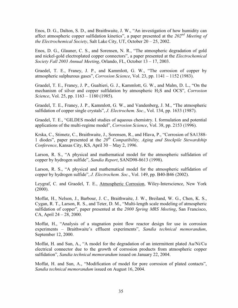
Figure 4 displays effect of time-integration scheme (Crank-Nicholson vs. backward Euler)

on solute-species mole-fraction profile along diffusion path at 90 seconds. The physical

parameters are those in the Base Case. As expected, the second-order accurate Crank-

Nicholson scheme yields better accuracy as compared with the first-order accurate

backward Euler method: the Goma prediction obtained using the Crank-Nicholson scheme

agrees perfectly well with the analytical solution whereas discrepancy between the Goma

prediction obtained using the backward Euler method and the analytical solution obviously

exists.

41

Figure 4. Effect of time-integration scheme on Goma prediction –


(16 elements, maximum time step = 0.1 second).

Figure 5. Effect of maximum time step on Goma prediction –


(16 elements, Crank-Nicholson time integration scheme).

Effect of Maximum Time Step

Figures 5 and 6 show the effects of maximum time step allowed in Goma computations on

solute-species mole-fraction profiles, respectively, along diffusion path at 90 seconds and

42

at the reaction plane as a function of time. The physical parameters are those in the Base

Case. Clearly, the Goma predictions agree perfectly with the analytical solution results only

when the maximum time step allowed is sufficiently small, e.g. 0.1 second. As presented in

Figure 7, CPU time required increases exponentially with decreasing maximum time step

allowed when it becomes desirably small.

Figure 6. Effect of maximum time step on Goma prediction –

solute-species mole fraction at reaction plane as a function of time


Figure 7. CPU time required as a function of maximum time step allowed

(16 elements, Crank-Nicholson time integration scheme, tim = 90 s).

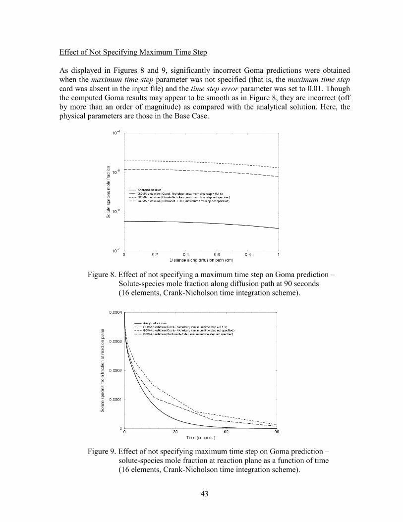
43

Effect of Not Specifying Maximum Time Step

As displayed in Figures 8 and 9, significantly incorrect Goma predictions were obtained

when the maximum time step parameter was not specified (that is, the maximum time step

card was absent in the input file) and the time step error parameter was set to 0.01. Though

the computed Goma results may appear to be smooth as in Figure 8, they are incorrect (off

by more than an order of magnitude) as compared with the analytical solution. Here, the

physical parameters are those in the Base Case.

Figure 8. Effect of not specifying a maximum time step on Goma prediction –

Solute-species mole fraction along diffusion path at 90 seconds


Figure 9. Effect of not specifying maximum time step on Goma prediction –

solute-species mole fraction at reaction plane as a function of time


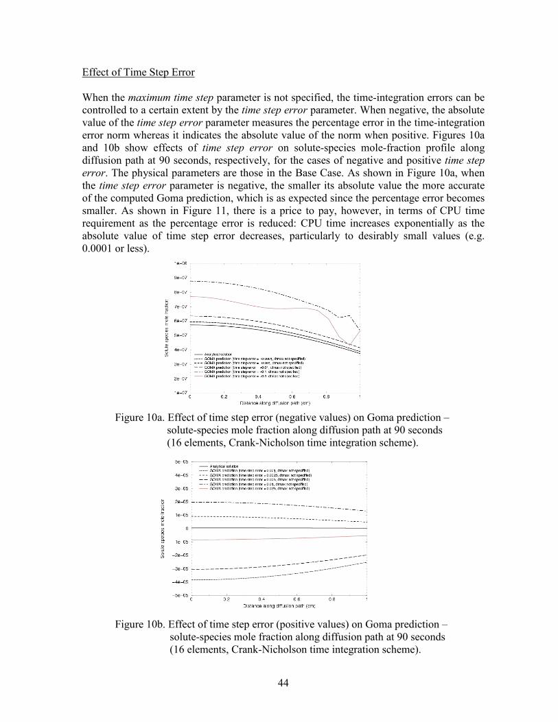
44

Effect of Time Step Error

When the maximum time step parameter is not specified, the time-integration errors can be

controlled to a certain extent by the time step error parameter. When negative, the absolute

value of the time step error parameter measures the percentage error in the time-integration

error norm whereas it indicates the absolute value of the norm when positive. Figures 10a

and 10b show effects of time step error on solute-species mole-fraction profile along

diffusion path at 90 seconds, respectively, for the cases of negative and positive time step

error. The physical parameters are those in the Base Case. As shown in Figure 10a, when

the time step error parameter is negative, the smaller its absolute value the more accurate

of the computed Goma prediction, which is as expected since the percentage error becomes

smaller. As shown in Figure 11, there is a price to pay, however, in terms of CPU time

requirement as the percentage error is reduced: CPU time increases exponentially as the

absolute value of time step error decreases, particularly to desirably small values (e.g.

0.0001 or less).

Figure 10a. Effect of time step error (negative values) on Goma prediction –



Figure 10b. Effect of time step error (positive values) on Goma prediction –



45

Figure 10c. Effect of time step error (positive values) on Goma prediction –

solute-species mole fraction at reaction plane at 90 seconds


Figure 11. CPU time required as a function of absolute value of time step error

(for the case of negative time step error, 16 elements,

Crank-Nicholson time integration scheme, time = 90 s).

Figures 10b and 10c show the effects of time step error when its value is positive. In this

case, no clear trend (in terms of reducing discrepancy between Goma prediction and

analytical solution) can be observed, suggesting that time step error when positive is not a

good parameter for controlling time integration errors.

Effect of Initial Time Step

Figures 12 and 13 show effects of initial time step on the computed Goma predictions of

solute-species mole fraction. The physical parameters are those in the Base Case. As

expected, effect of the initial time step is small for the range of values studied.

46

Figure 12. Effect of initial time step on Goma prediction – solute-species

mole fraction along diffusion path at 90 seconds


Figure 13. Effect of initial time step on Goma prediction –

solute-species mole fraction at reaction plane at 90 seconds


47

Summary and Conclusions

For the first time, effects of time-integration scheme and parameters on Goma predictions

was systematically studied using a time-dependent model problem for which analytical

solution can be obtained. The model problem involves a diffusion process with a dilute

solute species and a slow surface chemical reaction at one of the boundaries. It was found

that Goma predictions of solute-species concentration profiles agree perfectly well with

that given by the analytical solution when proper time-integration scheme and parameters

were employed. When inappropriate time-integration scheme or parameters were used,

however, significantly incorrect results were obtained. As expected, the second-order

accurate Crank-Nicholson time-integration scheme yielded more accurate predictions as

compared with the first-order accurate backward-Euler method. Of the parameters used by

Goma in time integration, the maximum-time-step parameter was found to be most effective

in reducing time-integration errors. As a rule of thumb, the maximum time step allowed

should be less than the time constant of the process, based on the limited findings in the

case study reported here. Lastly, effect of mesh refinement was also examined and it was

found that in modeling transient processes errors resulted from inappropriate use of time

integration scheme and parameters are much more significant than that from the

employment of an inadequately refined mesh (that is, errors from time integration are much

more pronounced than that from mesh refinement) based, again, on limited findings

presented in this appendix.

References

Crank, J., The Mathematics of Diffusion, Second Edition, Oxford University Press, New

York, NY (1975).

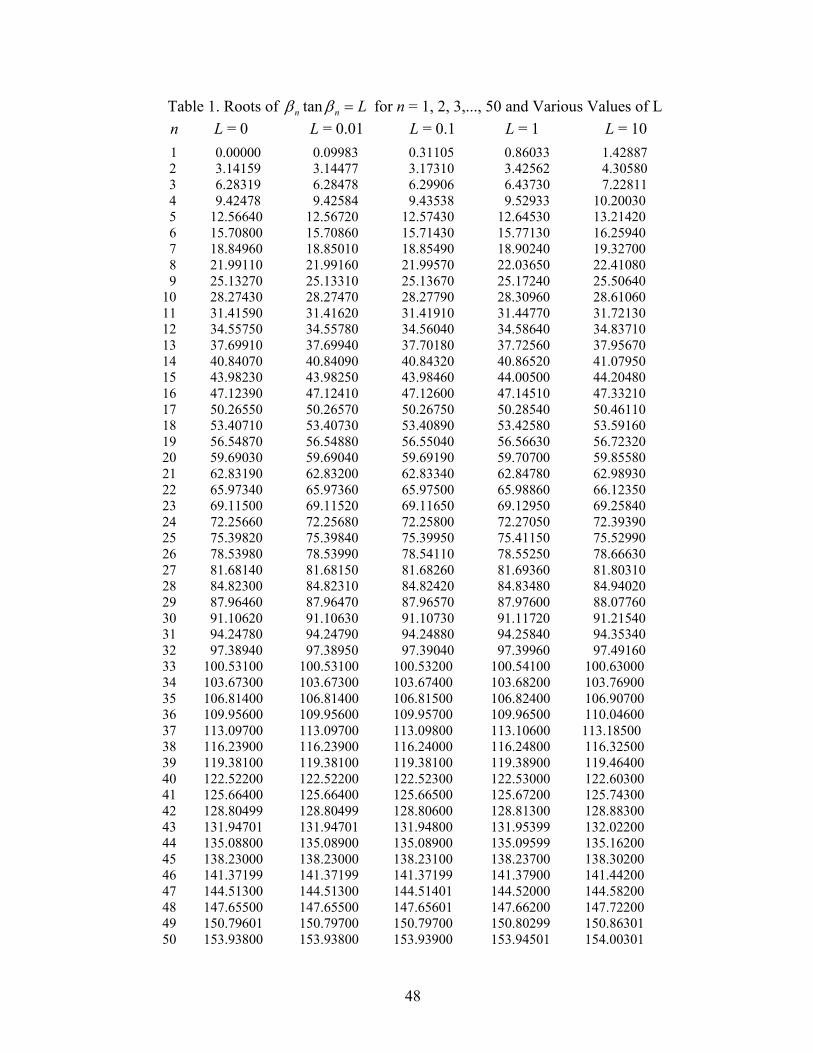
48

Table 1. Roots of Lnn =ββ tan for n = 1, 2, 3,..., 50 and Various Values of L

n L = 0 L = 0.01 L = 0.1 L = 1 L = 10

1 0.00000 0.09983 0.31105 0.86033 1.42887

2 3.14159 3.14477 3.17310 3.42562 4.30580

3 6.28319 6.28478 6.29906 6.43730 7.22811

4 9.42478 9.42584 9.43538 9.52933 10.20030

5 12.56640 12.56720 12.57430 12.64530 13.21420

6 15.70800 15.70860 15.71430 15.77130 16.25940

7 18.84960 18.85010 18.85490 18.90240 19.32700

8 21.99110 21.99160 21.99570 22.03650 22.41080

9 25.13270 25.13310 25.13670 25.17240 25.50640

10 28.27430 28.27470 28.27790 28.30960 28.61060

11 31.41590 31.41620 31.41910 31.44770 31.72130

12 34.55750 34.55780 34.56040 34.58640 34.83710

13 37.69910 37.69940 37.70180 37.72560 37.95670

14 40.84070 40.84090 40.84320 40.86520 41.07950

15 43.98230 43.98250 43.98460 44.00500 44.20480

16 47.12390 47.12410 47.12600 47.14510 47.33210

17 50.26550 50.26570 50.26750 50.28540 50.46110

18 53.40710 53.40730 53.40890 53.42580 53.59160

19 56.54870 56.54880 56.55040 56.56630 56.72320

20 59.69030 59.69040 59.69190 59.70700 59.85580

21 62.83190 62.83200 62.83340 62.84780 62.98930

22 65.97340 65.97360 65.97500 65.98860 66.12350

23 69.11500 69.11520 69.11650 69.12950 69.25840

24 72.25660 72.25680 72.25800 72.27050 72.39390

25 75.39820 75.39840 75.39950 75.41150 75.52990

26 78.53980 78.53990 78.54110 78.55250 78.66630

27 81.68140 81.68150 81.68260 81.69360 81.80310

28 84.82300 84.82310 84.82420 84.83480 84.94020

29 87.96460 87.96470 87.96570 87.97600 88.07760

30 91.10620 91.10630 91.10730 91.11720 91.21540

31 94.24780 94.24790 94.24880 94.25840 94.35340

32 97.38940 97.38950 97.39040 97.39960 97.49160

33 100.53100 100.53100 100.53200 100.54100 100.63000

34 103.67300 103.67300 103.67400 103.68200 103.76900

35 106.81400 106.81400 106.81500 106.82400 106.90700

36 109.95600 109.95600 109.95700 109.96500 110.04600

37 113.09700 113.09700 113.09800 113.10600 113.18500

38 116.23900 116.23900 116.24000 116.24800 116.32500

39 119.38100 119.38100 119.38100 119.38900 119.46400

40 122.52200 122.52200 122.52300 122.53000 122.60300

41 125.66400 125.66400 125.66500 125.67200 125.74300

42 128.80499 128.80499 128.80600 128.81300 128.88300

43 131.94701 131.94701 131.94800 131.95399 132.02200

44 135.08800 135.08900 135.08900 135.09599 135.16200

45 138.23000 138.23000 138.23100 138.23700 138.30200

46 141.37199 141.37199 141.37199 141.37900 141.44200

47 144.51300 144.51300 144.51401 144.52000 144.58200

48 147.65500 147.65500 147.65601 147.66200 147.72200

49 150.79601 150.79700 150.79700 150.80299 150.86301

50 153.93800 153.93800 153.93900 153.94501 154.00301

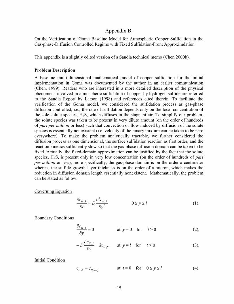
49

Appendix B.

On the Verification of Goma Baseline Model for Atmospheric Copper Sulfidation in the

Gas-phase-Diffusion Controlled Regime with Fixed Sulfidation-Front Approximdation

This appendix is a slightly edited version of a Sandia technical memo (Chen 2000b).

Problem Description

A baseline multi-dimensional mathematical model of copper sulfidation for the initial

implementation in Goma was documented by the author in an earlier communication

(Chen, 1999). Readers who are interested in a more detailed description of the physical

phenomena involved in atmospheric sulfidation of copper by hydrogen sulfide are referred

to the Sandia Report by Larson (1998) and references cited therein. To facilitate the

verification of the Goma model, we considered the sulfidation process as gas-phase

diffusion controlled, i.e., the rate of sulfidation depends only on the local concentration of

the sole solute species, H2S, which diffuses in the stagnant air. To simplify our problem,

the solute species was taken to be present in very dilute amount (on the order of hundreds

of part per million or less) such that convection or flow induced by diffusion of the solute

species is essentially nonexistent (i.e. velocity of the binary mixture can be taken to be zero

everywhere). To make the problem analytically tractable, we further considered the

diffusion process as one dimensional, the surface sulfidation reaction as first order, and the

reaction kinetics sufficiently slow so that the gas-phase diffusion domain can be taken to be

fixed. Actually, the fixed-domain approximation can be justified by the fact that the solute

species, H2S, is present only in very low concentration (on the order of hundreds of part

per million or less); more specifically, the gas-phase domain is on the order a centimeter

whereas the sulfide growth layer thickness is on the order of a micron, which makes the

reduction in diffusion domain length essentially nonexistent. Mathematically, the problem

can be stated as follow:

Governing Equation

2

2

22

y

cD

t

c SHSH

∂

∂=

∂

∂ ly ≤≤0 (1).

Boundary Conditions

02 =∂

∂

y

c SH at y = 0 for t > 0 (2),

SH

SHkc

y

cD

2

2 =∂

∂− at y = l for t > 0 (3),

Initial Condition

0,22 SHSH cc = at t = 0 for ly ≤≤0 (4).

50

In above SHc 2 is the molar concentration of H2S in units of moles/cm

3, y coordinate along

the diffusion path in units of cm, t time in units of second, D diffusion coefficient in units

of cm2/s, k first-order kinetic rate constant in units of cm/s, and l length of the fixed

diffusion domain in units of cm. In Equations 1 and 3 the Fick’s first law is used to relate

flux of the solute-species to its gradient, which is a very good approximation for systems

involving dilute solute species. Equation 2 simply states that there is no flux of H2S across

the non-reacting boundary (i.e., y = 0). This was chosen so that the analytical solution can

be cleanly obtained. Another possibility is to specify the concentration of H2S at y = 0.

Actually, a more general or appropriate boundary condition at y = 0 is to specify a non-zero

flux by using a mass-transfer coefficient, α:

)( ,22

2

bSHSH

SHcc

y

c−=

∂

∂α at y = 0 for t > 0 (5),

where bSHc ,2 is the concentration of H2S in the bulk (i.e., outside the boundary at y = 0). In

this case, the additional parameter needed to be specified is the mass-transfer coefficient, α,

which depends on the location of the boundary at y = 0.

Analytical Solution

As shown in Appendix A, Equation 1 along with the associated boundary and initial

conditions, Equations 2 - 4, can be solved analytically using the method of separation of

variables to yield the following exact solution (cf. Crank 1975, Equation 4.50 on page 60):

∑∞

=

−

++=

122

0 cos)(

)cos(22

2

n nn

l

Dt

n

LL

el

yL

c

c

n

ββ

ββ

(6),

where )/( DklL ≡ is a dimensionless parameter, and nβ , the eigenvalues, are given by

Lnn =ββ tan (7).

Values of nβ can be obtained by solving Equation 7 iteratively using Newton’s method and

they are listed in Table 1 of Appendix A for n = 1, 2, 3, …, 50 and L = 0.0, 0.01, 0.1, 1, 10.

From the mass balance on copper sulfide (Cu2S), we have

ArMdt

hAdSCuSCu

SCu

22

2 =ρ

(8),

51

rH2S

kcH2S y l=

kcxH2S y l=

= =

td

dh cMCu2S

ρCu2S

-------------------kxH2S y l==

where A is total area of the copper-substrate surface on which sulfidation occurs in units of

cm2, h the average thickness of the dense copper sulfide layer in unit of cm, SCu2

ρ density

of copper sulfide in units of g/cm3, SCuM

2 molecular weight of copper sulfide in units of

g/mole, and SCur 2 the rate of formation of copper sulfide in units of mole/cm

2-s. From

stoichiometry of the overall copper sulfidation reaction (cf. Larson 1998),

2Cu + H2S(g) + 2

1O2(g) →

Cu2S + H2O(l) (9),

we have SHSCu rr22

= where SHr 2 is the rate of consumption of H2S; that is, the rate of

formation of Cu2S is equal to the rate of consumption of H2S. Upon substitution, Equation

8 becomes

SCuSCu

SCurM

dt

hd

22

2 =ρ

(10).

With the first-order kinetics assumption stated previously, we have

(11),

where c is the total molar concentration of the air/H2S mixture and can be determined using

the ideal gas law (i.e., RT

pc = ; under normal condition of 1 atm and 25

oC, c = 4.09x10

-5

mol/cm3), SHx 2

the mole fraction of H2S. Combining Equations 10 and 11 yields

(12).

From Equation 6, we have

∑∞

=

−

++=

122

0, )(

22

2

2

2

n n

l

Dt

SH

SH

LL

Le

x

xn

β

β

(13).

Upon substituting Equation 13 into Equation 12 and subsequently integrating with the

initial condition of h = 0 at t = 0, we obtain the average copper sulfide layer thickness as a

function of time:

52

h ti( ) h ti 1–( )cMCu2S

ρCu2S

-------------------k xH2Sti( )

y l=xH2S

ti 1–( )y l=

+[ ]+=

∑∞

=

−

++

−

=1

222

2

0,)(

12)(

2

2

2

2

2

n nn

l

Dt

SH

SCu

SCu

LL

e

LxcM

l

th

n

ββρ

β

(14).

Goma Model Computation

Equation 1 along with boundary and initial conditions as specified in Equations 2 - 4 was

solved using Goma to yield SHx 2 as a function of time and spatial position. In the Goma

computation we used an evenly spaced 16-element mesh (only a single row of element in

the direction normal to the diffusion path was used in order to reduce CPU time

requirement, and the height of the elements was taken to be 0.02 cm) and a second-order

accurate Crank-Nicholson time-integration scheme with an initial time step of 10-9

second.

Effects of mesh refinement and time-integration scheme and parameters for this problem

have been studied and is documented in Appendix A. After computed SHx 2 with Goma, we

integrated Equation 12 numerically using Trapezoidal rule to yield the average thickness of

the copper sulfide layer at discrete time steps:

(15).

Results and Discussion

Comparisons of Goma prediction with analytical solution are presented in Figures 1 and 2,

respectively, for H2S solute species mole fraction on the sulfidation surface and average

sulfide layer thickness as functions of time under two different sets of transport/kinetic

properties and process condition. Clearly, the Goma predictions agree perfectly well with

the results from the analytical solution.

Effects of maximum time step allowed in Goma computations on H2S solute species mole

fraction on the sulfidation surface and average sulfide layer thickness are presented in

Figures 3 and 4, again, for two different sets of transport/kinetic properties and process

condition. When maximum time steps are sufficiently small, excellent agreements are seen

between Goma predictions and results from the analytical solution. When the maximum

time steps exceed threshold values, discrepancies arise, and they are significant when the

maximum time steps become relatively large. The effect of maximum time step on average

sulfide layer thickness is more pronounced than that on H2S solute species mole fraction

because the maximum time step further contributes to the discrepancy in the numerical

integration step that yields the average sulfide layer thickness once SHx 2 is computed.

53

Figure 1a. Comparison of Goma prediction with analytical solution – H2S solute- species mole fraction on the sulfidation surface as a function of time. (parameters: D = 0.1 cm

2/s, k = 0.1 cm/s, l = 1 cm, 0,2SHx = 400 ppm;

Crank-Nicholson scheme with a maximum time step of 0.05 second).

Figure 1b. Comparison of Goma prediction with analytical solution – average sulfide layer thickness as a function of time . (parameters: D = 0.1 cm

2/s, k = 0.1 cm/s, l = 1 cm, 0,2SHx = 400 ppm;


54

Figure 2a. Comparison of Goma prediction with analytical solution – H2S solute- species mole fraction on the sulfidation surface as a function of time. (parameters: D = 0.1 cm

2/s, k = 2 cm/s, l = 1 cm, 0,2SHx = 400 ppb;


Figure 2b. Comparison of Goma prediction with analytical solution – average sulfide layer thickness as a function of time . (parameters: D = 0.1 cm

2/s, k = 2 cm/s, l = 1 cm, 0,2SHx = 400 ppb;


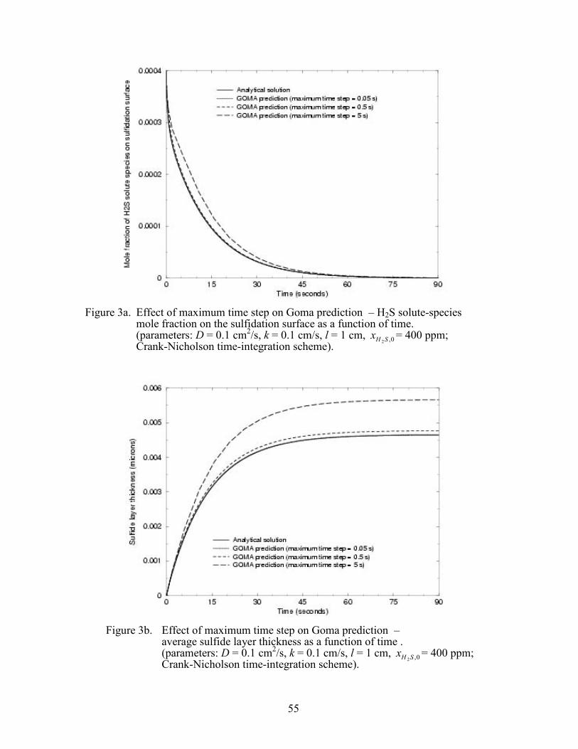
55

Figure 3a. Effect of maximum time step on Goma prediction – H2S solute-species mole fraction on the sulfidation surface as a function of time. (parameters: D = 0.1 cm

2/s, k = 0.1 cm/s, l = 1 cm, 0,2SHx = 400 ppm;

Crank-Nicholson time-integration scheme).

Figure 3b. Effect of maximum time step on Goma prediction – average sulfide layer thickness as a function of time . (parameters: D = 0.1 cm

2/s, k = 0.1 cm/s, l = 1 cm, 0,2SHx = 400 ppm;


56

Figure 4a. Effect of maximum time step on Goma prediction – H2S solute-species mole fraction on the sulfidation surface as a function of time. (parameters: D = 0.1 cm

2/s, k = 2 cm/s, l = 1 cm, 0,2SHx = 400 ppb;


Figure 4b. Effect of maximum time step on Goma prediction – average sulfide layer thickness as a function of time . (parameters: D = 0.1 cm

2/s, k = 2 cm/s, l = 1 cm, 0,2SHx = 400 ppb;


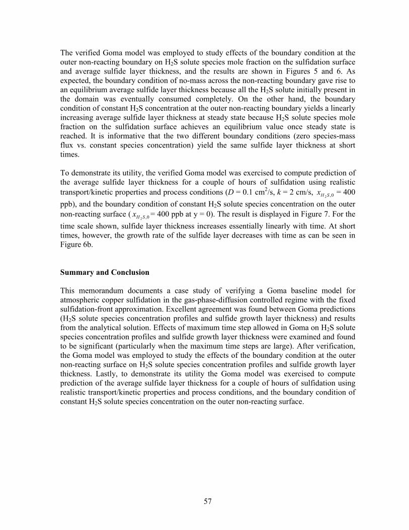
57

The verified Goma model was employed to study effects of the boundary condition at the

outer non-reacting boundary on H2S solute species mole fraction on the sulfidation surface

and average sulfide layer thickness, and the results are shown in Figures 5 and 6. As

expected, the boundary condition of no-mass across the non-reacting boundary gave rise to

an equilibrium average sulfide layer thickness because all the H2S solute initially present in

the domain was eventually consumed completely. On the other hand, the boundary

condition of constant H2S concentration at the outer non-reacting boundary yields a linearly

increasing average sulfide layer thickness at steady state because H2S solute species mole

fraction on the sulfidation surface achieves an equilibrium value once steady state is

reached. It is informative that the two different boundary conditions (zero species-mass

flux vs. constant species concentration) yield the same sulfide layer thickness at short

times.

To demonstrate its utility, the verified Goma model was exercised to compute prediction of

the average sulfide layer thickness for a couple of hours of sulfidation using realistic

transport/kinetic properties and process conditions (D = 0.1 cm2/s, k = 2 cm/s, 0,2SHx = 400

ppb), and the boundary condition of constant H2S solute species concentration on the outer

non-reacting surface ( 0,2SHx = 400 ppb at y = 0). The result is displayed in Figure 7. For the

time scale shown, sulfide layer thickness increases essentially linearly with time. At short

times, however, the growth rate of the sulfide layer decreases with time as can be seen in

Figure 6b.

Summary and Conclusion

This memorandum documents a case study of verifying a Goma baseline model for

atmospheric copper sulfidation in the gas-phase-diffusion controlled regime with the fixed

sulfidation-front approximation. Excellent agreement was found between Goma predictions

(H2S solute species concentration profiles and sulfide growth layer thickness) and results

from the analytical solution. Effects of maximum time step allowed in Goma on H2S solute

species concentration profiles and sulfide growth layer thickness were examined and found

to be significant (particularly when the maximum time steps are large). After verification,

the Goma model was employed to study the effects of the boundary condition at the outer

non-reacting surface on H2S solute species concentration profiles and sulfide growth layer

thickness. Lastly, to demonstrate its utility the Goma model was exercised to compute

prediction of the average sulfide layer thickness for a couple of hours of sulfidation using

realistic transport/kinetic properties and process conditions, and the boundary condition of

constant H2S solute species concentration on the outer non-reacting surface.

58

Figure 5a. Effect of boundary condition at the outer non-reacting boundary (y=0) on H2S solute-species mole fraction on the sulfidation surface. (parameters: D = 0.1 cm

2/s, k = 0.1 cm/s, l = 1 cm, 0,2SHx = 400 ppm;

Crank-Nicholson scheme with maximum time step of 0.05 second).

Figure 5b. Effect of boundary condition at the outer non-reacting boundary (y=0) on the average sulfidae thickness. (parameters: D = 0.1 cm

2/s, k = 0.1 cm/s, l = 1 cm, 0,2SHx = 400 ppm;


59

Figure 6a. Effect of boundary condition at the outer non-reacting boundary (y=0) on H2S solute-species mole fraction on the sulfidation surface. (parameters: D = 0.1 cm

2/s, k = 2 cm/s, l = 1 cm, 0,2SHx = 400 ppb;


Figure 6b. Effect of boundary condition at the outer non-reacting boundary (y=0) on the average sulfidae thickness. (parameters: D = 0.1 cm

2/s, k = 2 cm/s, l = 1 cm, 0,2SHx = 400 ppb;


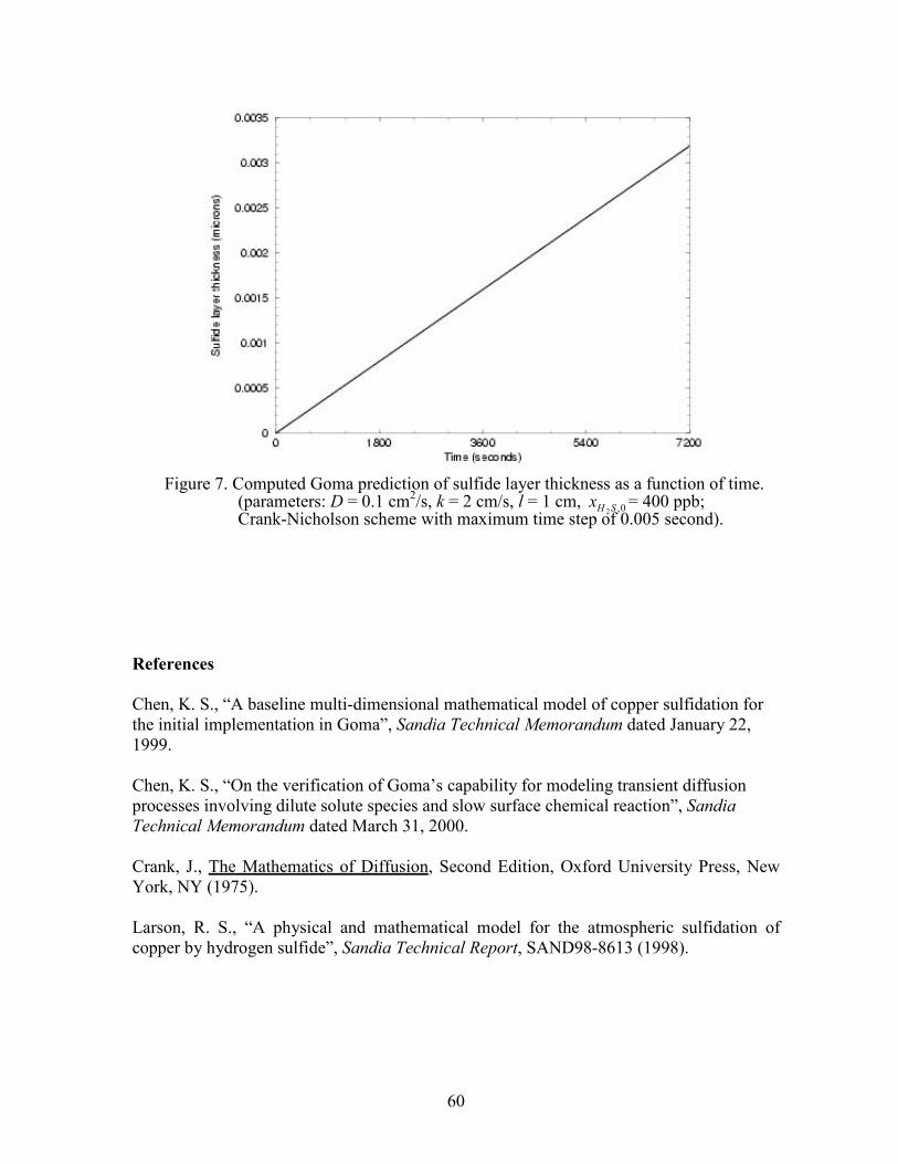
60

Figure 7. Computed Goma prediction of sulfide layer thickness as a function of time. (parameters: D = 0.1 cm

2/s, k = 2 cm/s, l = 1 cm, 0,2SHx = 400 ppb;


References

Chen, K. S., “A baseline multi-dimensional mathematical model of copper sulfidation for

the initial implementation in Goma”, Sandia Technical Memorandum dated January 22,

1999.

Chen, K. S., “On the verification of Goma’s capability for modeling transient diffusion

processes involving dilute solute species and slow surface chemical reaction”, Sandia

Technical Memorandum dated March 31, 2000.

Crank, J., The Mathematics of Diffusion, Second Edition, Oxford University Press, New

York, NY (1975).


copper by hydrogen sulfide”, Sandia Technical Report, SAND98-8613 (1998).

61

9. DISTRIBUTION

MS 0384 9140 H. S. Morgan

MS 0825 9110 W. H. Hermina

MS 0834 9112 J. E. Johannes

MS 0827 9113 P. A. Sackinger

MS 0834 9114 J. S. Lash

MS 0834 9114 T. A. Baer

MS 0834 9114 K. S. Chen (5)

MS 0834 9114 H. K. Moffat

MS 0382 9114 P. K. Notz

MS 0834 9114 R. R. Rao

MS 0834 9114 R. A. Roach

MS 0834 9114 P. R. Schunk

MS 0834 9114 A. C.-T. Sun

MS 0889 1861 J. W. Braithwaite

MS 0889 1832 F. D. Wall

MS 0888 1832 D. G. Enos

MS 0889 1832 N. R. Sorensen

MS 1415 1110 J. C. Barbour

MS 1415 1112 N. A. Missert

MS 1415 1112 J. P. Sullivan

MS 0750 6118 L. J. Criscenti

MS 0750 6118 R. T. Cygan

MS 0748 6863 F. Gelbard

MS 9042 8752 C. D. Moen

MS 9042 8752 R. S. Larson

MS 9018 8945-1 Central Technical Files

MS 0899 9616 Technical Library

multi-dimensional modeling of atmospheric copper...

Documents