MTAT.03.227 Machine Learning (Spring 2013)

Exercise session XIV: Support Vector Machines

Konstantin Tretyakov

May 13, 2013

The aim of this exercise session is to get acquainted with the inner workingsof support vector machine classification and regression. As usual, for all exercisesyou need to write a brief explanation and, for most of them, also a short piece ofcode demonstrating the result. You can submit your whole solution as a singledecently commented R file, provided it is sequentially readable and executable.

We shall use a slightly modified version of the familiar base code from Ex-ercise Session VI. Fetch it at svm base.R.

Exercise 1 (2pt). We begin by analyzing a trivialized dataset consisting of Maximal mar-ginjust four points. Use the functions load.data and plot.data to visualize it.

Use manual examination of the data to derive the parameters (w, b) of thecanonical1 maximal-margin classifier.

Hints.

1. Use pen and paper to sketch the location of the maximal margin separat-ing hyperplane for the given dataset and its two margin-defining isolinesf(x) = ±1.

2. By visual examination, guess the coordinates of the weight vector w (upto a constant). Use plot.classifier(w) and plot.data(data, add=T)

to verify your guess.

3. Next, find the length of the normal, |w|, such that would assure that theclosest training points are located at the isolines ±1. For this, note thatthe distance between those two isolines is equal to d = 2/|w|.

4. Rescale the w you guessed in Step 2 to have length you computed inStep 3.

5. Finally, compute the value for the bias parameter b by using the fact thatf(x1) = −1.

6. Visualize the computed (w, b) using plot.classifier.

1A canonical maximal-margin classifier is the classifier for which the functional margin ofthe closest training example is equal to 1. It is what we were talking about on the lecture.

1

Solution.

1. A brief look at the data should convince you that what we are looking foris the following separating hyperplane:

2. The normal of the separating hyperplane seems to be exactly diagonal,hence the direction of the normal is given by w = (1, 1)T .

3. Looking at the figure above we can compute that the geometric distanced between the two desired margins is 2

√2. The desired normal vector w

must therefore have length |w| = 2/d = 1/√

2.

4. The length of our first guess, (1, 1)T is√

2, hence we have to scale it by afactor of 1/2 to obtain w = (0.5, 0.5)T , which has the required length.

5. Now that we know w we can find the bias w0, which positions the sepa-rating line so that the first training example x1 = (1, 1) is exactly at theisoline f(x) = −1. For that we simply solve:

f(x1) = −1

wTx1 + w0 = −1

(0.5, 0.5) ·(

11

)+ w0 = −1

0.5 + 0.5 + w0 = −1

w0 = −2.

2

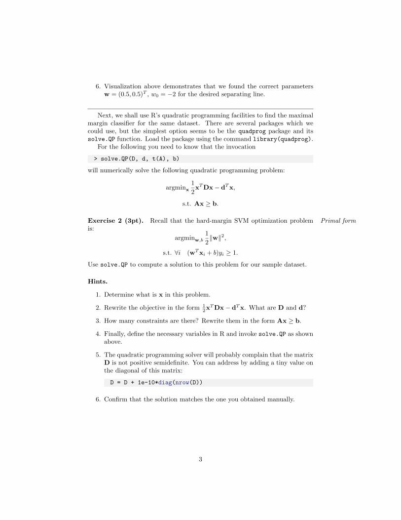
6. Visualization above demonstrates that we found the correct parametersw = (0.5, 0.5)T , w0 = −2 for the desired separating line.

Next, we shall use R’s quadratic programming facilities to find the maximalmargin classifier for the same dataset. There are several packages which wecould use, but the simplest option seems to be the quadprog package and itssolve.QP function. Load the package using the command library(quadprog).

For the following you need to know that the invocation

> solve.QP(D, d, t(A), b)

will numerically solve the following quadratic programming problem:

argminx

1

2xTDx− dTx,

s.t. Ax ≥ b.

Exercise 2 (3pt). Recall that the hard-margin SVM optimization problem Primal formis:

argminw,b

1

2‖w‖2,

s.t. ∀i (wTxi + b)yi ≥ 1.

Use solve.QP to compute a solution to this problem for our sample dataset.

Hints.

1. Determine what is x in this problem.

2. Rewrite the objective in the form 12x

TDx− dTx. What are D and d?

3. How many constraints are there? Rewrite them in the form Ax ≥ b.

4. Finally, define the necessary variables in R and invoke solve.QP as shownabove.

5. The quadratic programming solver will probably complain that the matrixD is not positive semidefinite. You can address by adding a tiny value onthe diagonal of this matrix:

D = D + 1e-10*diag(nrow(D))

6. Confirm that the solution matches the one you obtained manually.

3

Solution.

1. We need to find the parameters w0 and w. The optimization variable xis thus a concatenation of the two: x := (w0,w

T ) = (w0, w1, w2)T .

2. Observe that

1

2‖w‖2 =

1

2wTw =

1

2wT

(1 00 1

)w =

1

2(w0,w

T )

0 0 00 1 00 0 1

(w0

w

),

and thus

D =

0 0 00 1 00 0 1

, d =

000

.

3. There is a single constraint for each data point, thus there is a total offour constraints. Let us rearrange them into the form Ax ≥ b:

(wTx1 + w0)y1 ≥ 1

(wTx2 + w0)y2 ≥ 1

(wTx3 + w0)y3 ≥ 1

(wTx4 + w0)y4 ≥ 1

⇔

(y1, y1xT1 )

(w0

w

)≥ 1

(y2, y2xT2 )

(w0

w

)≥ 1

(y3, y3xT3 )

(w0

w

)≥ 1

(y4, y4xT4 )

(w0

w

)≥ 1

⇔

y1 y1x

T1

y2 y2xT2

y3 y3xT3

y4 y4xT4

(w0

w

)≥

1111

4-6. data = load.data()

D = diag(3)

D[1, 1] = 0

D = D + 1e-10*diag(3)

d = c(0, 0, 0)

A = cbind(data$y, data$X * data$y)

b = c(1, 1, 1, 1)

library(quadprog)

sol = solve.QP(D, d, t(A), b)

> sol$solution

[1] -2.0 0.5 0.5

4

Exercise 3 (3pt). Now let us solve the SVM in dual form. Some formalities Dual formaside, the dual form is obtained by representing the weight vector w as a linearcombination of training points:

w =∑i

αiyixi,

where αi are the unknowns (the dual variables) we shall be seeking for insteadof w.

In the dual form the optimization problem turns into2:

argminα

(1

2αT (K ◦Y)α− 1Tα

)

s.t. α ≥ 0,

yTα = 0,

where

K = XXT is the kernel matrix ,

Y = yyT ,

1 is a vector of ones, and

◦ denotes elementwise multiplication.

Recast this formulation in the format suitable for solve.QP and find both thedual solution α and the corresponding bias term b. Finally, use the obtained αvalues to compute w and compare your result to two previous attempts.

Hints.

1. Similarly to the previous exercise, you first need to recast the problemin terms of D, d, A, b. Note that there is one equality constraint now.Include its coefficients as the first row of the matrix A, its right side as thefirst element of vector b and provide the parameter meq=1 to solve.QP.

2. Similarly to the previous exercise, if the solver complains about the lackof positive semidefiniteness, add a small value to the diagonal of D.

3. Compute w as

w =∑i

αiyixi.

Note that this can be done concisely matrix multiplication.

2Note that in the lecture there was also the constraint α ≤ C. This constraint is notpresent in the hard-margin case, however.

5

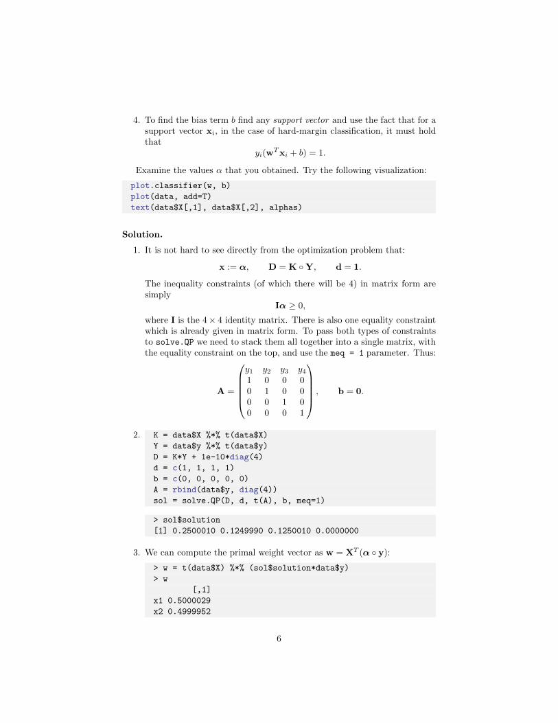
4. To find the bias term b find any support vector and use the fact that for asupport vector xi, in the case of hard-margin classification, it must holdthat

yi(wTxi + b) = 1.

Examine the values α that you obtained. Try the following visualization:

plot.classifier(w, b)

plot(data, add=T)

text(data$X[,1], data$X[,2], alphas)

Solution.

1. It is not hard to see directly from the optimization problem that:

x := α, D = K ◦Y, d = 1.

The inequality constraints (of which there will be 4) in matrix form aresimply

Iα ≥ 0,

where I is the 4× 4 identity matrix. There is also one equality constraintwhich is already given in matrix form. To pass both types of constraintsto solve.QP we need to stack them all together into a single matrix, withthe equality constraint on the top, and use the meq = 1 parameter. Thus:

A =

y1 y2 y3 y41 0 0 00 1 0 00 0 1 00 0 0 1

, b = 0.

2. K = data$X %*% t(data$X)

Y = data$y %*% t(data$y)

D = K*Y + 1e-10*diag(4)

d = c(1, 1, 1, 1)

b = c(0, 0, 0, 0, 0)

A = rbind(data$y, diag(4))

sol = solve.QP(D, d, t(A), b, meq=1)

> sol$solution

[1] 0.2500010 0.1249990 0.1250010 0.0000000

3. We can compute the primal weight vector as w = XT (α ◦ y):

> w = t(data$X) %*% (sol$solution*data$y)

> w

[,1]

x1 0.5000029

x2 0.4999952

6

4. A support vector (for the hard margin case) is any training example withthe corresponding α 6= 0. We can use any of them to compute w0.

support_vectors = which(sol$solution != 0) # 1, 2, 3

s = support_vectors[1] # Pick any

w0 = data$y[s] - t(w) %*% data$X[s,] # -1.999998

By examining the α values of the support vectors, observe how the “weight”of the constraints is balanced on both sides of the separating line.

Exercise 4* (5pt). In the case of hard-margin classification you may always Finding thebias term indual

find w0 by relying on the fact that all support vectors are always located ex-actly on the margin (i.e. they satisfy f(xi) = yi). In the case of soft marginclassification this idea can also sometimes be exploited. Namely, all supportvectors which have 0 < α < C are also necessarily on the margin. However, thisneed not always be the case – it may turn out so that all support vectors of asoft-margin SVM are violating the margin.

How should you compute w0 in this case? Provide a proof of your claim.

Solution. Consider the primal form of the soft-margin SVM optimizationtask:

argminw,w0

1

2‖w‖2 + C

∑i

(1− (wTxi + w0)yi)+

After we have found the dual solution α, we can use it to compute and fixthe correct weight vector w := w∗. We then consider the optimization problemagain with a fixed value of w, this time to find just the bias term:

argminw0

1

2‖w∗‖2 + C

∑i

(1− (w∗Txi + w0)yi)+.

We can simplify it by observing that for the purposes of optimization withrespect to w0, the (now fixed) value of ‖w∗‖2 plays no role. In addition, we candrop all those terms from the sum, which correspond to non-support vectors xi,as we know that those play no role in determining the separating line, as longas they lie outside the margin:

argminw0

∑s∈SV

(1− (w∗Txs + w0)ys)+.

s.t. ∀k /∈ SV (w∗Txk + w0)yk ≥ 1 (*)

Next, note that for all support vectors the expression 1− (w∗Txs +w0)ys at theoptimal value of w0 is always non-negative. We can thus safely replace the (·)+function with | · |, which is “more stringent” for negative inputs only.

argminw0

∑s∈SV

|1− (w∗Txs + w0)ys|.

7

We rearrange slightly:

|1− (w∗Txs + w0)ys| = |ys − (w∗Txs + w0)| = |(ys −w∗Txs)− w0|,

and see that the final optimization is just the min-absolute-value problem:

argminw0

∑s∈SV

|es − w0|.

where es = ys −w∗Txs.We know from Exercise Session V that the solution to this problem is the

median of es. Thus, the correct way to obtain w0 is to compute es for all supportvectors, and take a median.

The additional condition (*) can sometimes play a role. Namely, when thenumber of support vectors is even3, the median is not uniquely defined – it is arange of values, some of which may not satisfy the condition (*).

The fact that the bias term w0 may not be uniquely defined has an intuitiveexplanation. Indeed, if there are no support vectors on the margin, then shiftingthe line slightly will decrease penalty paid by the support vectors on one side,and compensate it by increasing the penalty of the support vectors on the otherside by exactly the same amount. Thus any positions of the separating lineare allowed, as long as support vectors are within the margins and non-supportvectors – outside the margins.

This suggests a practical way of computing the bias term directly from theconstraints. We know that{

yi(w∗Txi + b) ≤ 1, for i ∈ SV,

yi(w∗Txi + b) ≥ 1, for i /∈ SV,

which can be written compactly as

yi(w∗Txi + b)

SV

≶ 1.

Then, multiplying both sides by yi and keeping track of the sign:w∗Txi + bSV≶ yi, if yi = 1

w∗Txi + bSV≷ yi, if yi = −1.

which, abusing notation even further, is:

w∗Txi + bSV xor −1

≶ yi,

bSV xor −1

≶ yi −wTxi,

3This, by the way, is a necessary condition for a situation where no support vectors are onthe margin, think why.

8

and thus the complete solution for b (in the case of no support vectors being onthe margin) is:

b ∈[

maxi∈LB

ei, mini∈UB

ei

],

where

UB = {i : i ∈ SV xor yi = −1},LB = {i : i /∈ SV xor yi = −1},ei = yi −w∗Txi.

It is worth noting that some implementations use the mean of es as theestimate of w0 rather than the median4 (which is correct for L2-SVMs, but notfor the “classical”, L1-SVMs).

Exercise 5 (1pt). Finally, let us use a third-party tool to fit an SVM model. e1071The de-facto standard implementation in R is provided by the package e1071

and its svm function5. Invoke it as follows:

m = svm(data$X, data$y, scale=FALSE,

kernel="linear", type="C-classification", cost=9e9)

Examine the output. Find the α vector and the bias term. Do they match yourprevious results? Compute the w vector.

Solution.

m = svm(data$X, data$y, scale=FALSE,

kernel="linear", type="C-classification", cost=9e9)

alphas = m$coefs # Only nonzero alphas in this vector

w = t(m$SV)%*% alphas

w0 = -m$rho

You might notice that the svm function internally reverses the classes – this isa consequence of treating y as a factor and its first value (which in our case is−1) as the positive class.

Exercise 6 (1pt). So far we have only examined hard-margin classification Soft-margin(note that the svm function does not have a specific hard-margin mode, butspecifying C = 9 ·109, as we did in the previous exercise, is more-or-less as goodas prohibiting any margin violations). Now let us study the effect of “relaxing”the margin.

First, add a new datapoint x5 = (0, 5)T of class y5 = −1 to the dataset:

4Probably because the topic of computing w0 is swept under the rug in many SVM textbooktreatments.

5This is actually a packaged version of the LibSVM C library.

9

data = load.data()

data$X = rbind(data$X, c(0, 5))

data$y = c(data$y, -1)

Now run svm with cost = 9e9 and plot the resulting classifier usingplot.classifier and plot.data. Try to guess what happens to the separatingline once you reduce the cost to 1 and then further to 0.1. Verify your guesses.

Solution. As we reduce the cost of misclassification slightly (say, to 10 orso), at first nothing changes. However, at some point, as the cost becomes smallenough, the SVM decides to “let go” of the single “most annoying” trainingexample (#2 in our case) in return for getting a wider margin. If we continuereducing the penalty, at some point another example will be sacrificed, and soon. Such “incremental letting go” of the parameters is actually a property of allmodels which involve sharp corners (like the hinge loss does) in their objectivefunction.

You may observe that one of the negative effects of having a very low regu-larization penalty is reduction in the sparseness of the model – the more trainingexamples are allowed to violate the margin, the larger is the total number ofsupport vectors.

On the other hand (this is something you do not see in this example but iscommonly observed on large datasets), the less stringent is the margin penalty,the faster will the SVM optimizer converge.

Exercise 7* (2pt). A kernel (to be covered in the upcoming lecture) is a RBF kernelgeneralization of an inner product. It turns out that everywhere where we usean inner product xT

i xj , we may instead use a nonlinear function K(xi,xj),which will serve the same purpose but will make our model non-linear.

One of the most popular kernels is the RBF kernel:

K(xi,xj) = exp(−γ‖xi − xj‖2

).

Study its properties on our toy example and answer the following questions.

1. The linear SVM in dual form, as you should know, corresponds to thefollowing functional:

f(x) =∑i

αiyixTi x + w0.

Is this functional linear in x? Prove it.

2. What is the corresponding functional of an SVM with an RBF kernel? Isit linear in x?

3. What is the value of K(x, z) for any point z that is geometrically veryclose to x? What is the value of K(x, z) for points z that are far from x?

10

4. Use the svm function to train an SVM classifier with an RBF kernel forthe data you used in the previous exercise. Let γ = 1 and C = 9 · 109.

5. Use the function plot.svm.functional, provided in the base code, tovisualize the resulting functional6. Locate the decision boundary on theresulting plot.

6. Try different values of γ ∈ {0.001, 0.01, 0.1, 1, 10} and visualize the results.What do you observe?

7. For γ = 0.1 try different values of C ∈ {0.1, 1, 10}. What do you observe?

8. What, do you think, is a good way for picking suitable values of γ and Cin real-life applications?

Solution.

1. Recall that a functional is linear if it satisfies f(ax + y) = af(x) + f(y).It is easy to see that the given functional does not satisfy this property(unless w0 = 0). However, it is none the less an affine functional andcorresponds to a linear classifier.

2. In the case of the RBF kernel, the functional has the form:

f(x) =∑i

αiyiK(xi,x) + w0 =∑i

αiyi exp(−γ‖xi − x‖2) + w0,

and is obviously not linear in x.

3. The function K(x, ·) is essentially a “hump” centered at x. For a pointz close to the center of the hump, the value of K(x, z) is close to 1. Forpoints z far from the center of the hump the value of K(x, z) is close to 0.This can provide some intuitive understanding of how the RBF classifierworks. Ignoring the w0 term it is essentially,

f(z) =∑i

αiyiK(xi, z) ≈∑i

yi = 1z is close to xi

αi −∑j

yj = −1z is close to xj

αj ,

Intuitively, the classifier sums the contributions α from the support vec-tors near the query point, and decides on its class based on what classdominates among the nearby highly contributing support vectors.

4-5. The training and visualization of the RBF model is performed as follows:

6Note that there is a function plot.svm in the e1071 package, but it does not exactly dowhat we need here.

11

m = svm(data$X, data$y, kernel="radial",

type="C-classification", gamma=1, cost=9e9)

plot.svm.functional(m, data)

Notice that the decision boundary is curved now, and that all data pointsare support vectors. Examine which isolines the datapoints are locatedat.

6. The following is a visualization of the resulting RBF functional for severalvalues of γ. Notice that small values of γ correspond to simpler decisionboundaries and smaller number of support vectors (i.e. high bias, lowvariance situation), whereas very high values of γ correspond to severeoverfitting.

7. What you should notice from varying the C parameter is that in our

12

situation it does not influence the general shape of the functional as muchas the γ parameter does (a fairly common effect with RBF SVMs). It does,however, affect the decision boundary – for very small C the classifier willsimply classify everything as the dominant class.

8. The most popular way of selecting the γ and C parameters is via cross-validation. Note that choosing two parameters means that we have toassess the algorithm performance for all pairs of (γ,C), from a preselectedgrid. This can often be quite computation-intensive.

Exercise 8* (1pt). In the lecture we did not get to cover the concept of Support vectorregressionSupport vector regression (SVR). Read about this approach on your own. As

the answer to this exercise, provide the formulation of the SVR optimizationproblem in primal form, explaining the meaning of the parameters.

Solution. Support vector regression differs from support vector classificationin that yi are not +1/− 1 class labels but rather arbitrary real values, and thatthe hinge loss penalty is replaced by the ε-insensitive loss penalty.

lossε(xi, yi) = (|yi − (wTxi + w0)| − ε)+.

Here ε defines the distance that the regression line may have to the true yivalues without incurring any penalty.

The optimization objective is then the familiar combination:

argminw,w0

1

2‖w‖2 + C

∑lossε(xi, yi).

Of course, analogously to the usual SVMs, there is an easily kernelizabledual reformulation.

Exercise 9* (2pt). Finally, let us consider a simple case study. We shall use Case studythe spam dataset from the package ElemStatLearn:

> install.packages("ElemStatLearn")

> library(ElemStatLearn)

> data(spam)

Each row in the spam data frame corresponds to an email. The emails havebeen preprocessed and frequencies of certain words have been extracted – thosefrequencies form the input features. You need to train a classifier to predict thevalue of the output feature (the spam attribute).

Leave 25% of the training examples for final testing, and use the 75% fortraining. Try SVM and at least one other classifier. For SVM, try at least thelinear and the RBF kernel and do not forget to tune the the gamma and cost

parameters. Explain how you proceeded. Once you settle on the best model,evaluate it once on your held-out 25% and report the result.

13

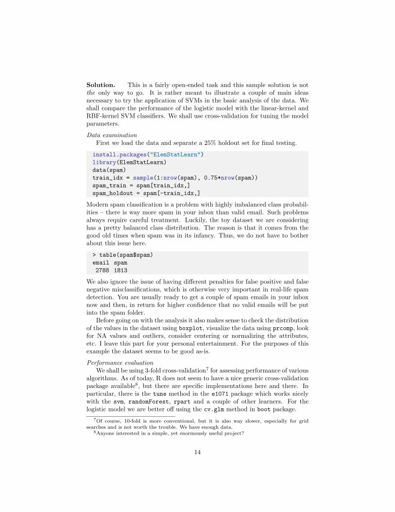
Solution. This is a fairly open-ended task and this sample solution is notthe only way to go. It is rather meant to illustrate a couple of main ideasnecessary to try the application of SVMs in the basic analysis of the data. Weshall compare the performance of the logistic model with the linear-kernel andRBF-kernel SVM classifiers. We shall use cross-validation for tuning the modelparameters.

Data examinationFirst we load the data and separate a 25% holdout set for final testing.

install.packages("ElemStatLearn")

library(ElemStatLearn)

data(spam)

train_idx = sample(1:nrow(spam), 0.75*nrow(spam))

spam_train = spam[train_idx,]

spam_holdout = spam[-train_idx,]

Modern spam classification is a problem with highly imbalanced class probabil-ities – there is way more spam in your inbox than valid email. Such problemsalways require careful treatment. Luckily, the toy dataset we are consideringhas a pretty balanced class distribution. The reason is that it comes from thegood old times when spam was in its infancy. Thus, we do not have to botherabout this issue here.

> table(spam$spam)

email spam

2788 1813

We also ignore the issue of having different penalties for false positive and falsenegative misclassifications, which is otherwise very important in real-life spamdetection. You are usually ready to get a couple of spam emails in your inboxnow and then, in return for higher confidence that no valid emails will be putinto the spam folder.

Before going on with the analysis it also makes sense to check the distributionof the values in the dataset using boxplot, visualize the data using prcomp, lookfor NA values and outliers, consider centering or normalizing the attributes,etc. I leave this part for your personal entertainment. For the purposes of thisexample the dataset seems to be good as-is.

Performance evaluationWe shall be using 3-fold cross-validation7 for assessing performance of various

algorithms. As of today, R does not seem to have a nice generic cross-validationpackage available8, but there are specific implementations here and there. Inparticular, there is the tune method in the e1071 package which works nicelywith the svm, randomForest, rpart and a couple of other learners. For thelogistic model we are better off using the cv.glm method in boot package.

7Of course, 10-fold is more conventional, but it is also way slower, especially for gridsearches and is not worth the trouble. We have enough data.

8Anyone interested in a simple, yet enormously useful project?

14

For simplicity of this exposition, we shall use the classification error (i.e.1 − accuracy) as our target performance measure, although it must be notedagain, that in tasks such as spam classification, precision and recall usuallymatter more than accuracy.

Classifier learning and parameter tuningLet us start with the logistic model.

m = glm(spam~., spam_train, family=binomial)

cv.results = cv.glm(spam_train, m,

function(y, yhat) { mean(y!=round(yhat)) }, 3)

cv.results$delta[1] # 0.07652174

The result is approximately 7.7%. Given that the size of the datasetnrow(spam train) used to perform cross-validation is 3450, we should remem-ber to treat this estimate as having a potential error of about ≈ 1/

√3450 ≈ 1.7%

or so9.Logistic regression does not have any tunable parameters, but we could

further experiment by attempting to apply logistic regression on transformed(e.g. log-transformed) data. I’ll leave it for your personal examination.

Next, let’s try linear SVMs:

tune.results = tune(svm, spam~., data=spam_train,

tunecontrol=tune.control(cross=3),

ranges=list(kernel="linear"))

The result is a similar 7.9%. What about RBF SVM? Let us check it with arange of values10 for γ ∈ {0.001, 0.01, 0.1} and11 C ∈ {1, 10, 100}:

tune.results = tune(svm, spam~., data=spam_train,

tunecontrol=tune.control(cross=3),

ranges=list(kernel="radial",

gamma=c(0.001, 0.01, 0.1),

cost=c(1, 10, 100)))

> tune.results

Parameter tuning of ’svm’:

- sampling method: 3-fold cross validation

- best parameters:

kernel gamma cost

9To be more precise, the 95% confidence interval of this estimate is±1.96

√0.9(1 − 0.9)/n ≈ ±1%.

10The small ranges are selected to allow the example to run in reasonable time. In practiceyou might often want to check larger parameter spaces and leave the evaluation running fora night or two. Sometimes a week or two.

11I should admit I made a couple of preliminary runs to rule out large γ and small C values.

15

radial 0.001 100

- best performance: 0.06840792

This result is only slightly (but most probably statistically significantly) betterthan the linear solutions, hence we settle on it as our best choice.

We can now perform the final evaluation of the selected model by trainingit on the whole training set and evaluating on the held-out set:

m = svm(spam~., spam_train, kernel="radial",

gamma=0.001, cost=100)

p = predict(m, spam_holdout)

performance = mean(p != spam_holdout$spam) # 0.05299739

Nice. Can we do even better on this dataset? Yes, we can, but using somethingelse than SVMs! Want to know how? Look for the answer in the textbook“Elements of Statistical Learning” by Hastie et al. 12.

12http://www.stanford.edu/~hastie/local.ftp/Springer/OLD/ESLII_print4.pdf

16