MSU Solar Physics NSF REU

Montana State University Bozeman, MT 59717

By

Chace K. Carlson

Submitted to Professor James Helbling College of Engineering

Embry-Riddle Aeronautical University July 8, 2016

Introduction

The Montana State University (MSU) Solar Physics Department conducts cutting edge

research studying the sun. Research involves analysis from many existing satellites such as

Yohkoh, SOHO, TRACE, RHESSI, Hinode, SDO, and IRIS. To supplement this research, the

physics department at MSU has created a Space Science and Engineering Laboratory (SSEL).

Dr. Dave Klumpar, director and research professor, heads this lab. The lab combines students of

many disciplines, including Physics, Electrical Engineering, Computer Science, and Mechanical

Engineering. Together these students, along with their mentors, are able to propose, design,

build, and test satellites that are sent to space year after year. Once these satellites are in space,

the SSEL uses it’s Space Operations Center (SOC) to communicate and recover scientific data.

I am involved in this program through the National Science Foundation’s (NSF) Research

Experiences for Undergrads (REU) program. This program aims to help undergraduate students

gain research experience who are preparing for graduate school. My expertise is the mechanical

engineering (ME) aspect of satellite projects, specifically the Guidance, Navigation, and Control

(GNC) subsystems. GNC Engineers work on two aspects of satellite projects, Attitude

Determination and Control Systems (ADACS) and Trajectory Planning and Propagation

Calculations. ADACS systems help in determining and controlling a spacecraft’s orientation in

3D space. Trajectory planning consists of planning a spacecraft’s orbit, and propagation consists

of predicting a spacecraft’s future orbit based off of its’ current orbit.

IT-SPINS

I’ve worked GNC on three different missions already, the first of which is the

Ionospheric-Thermospheric Scanning Photometer for Ion-Neutral Studies (IT-SPINS). Its

mission is to provide the first 2D tomographic imaging from a 3U research Cube Sat. It is also

MSU’s first Cube Sat with an active ADACS system. It will carry Stanford Research Institute

International’s CTIP measuring device, and is planned to launch on October 17, 2017 on NASA

Educational Launch of Nanosatellites (ELaNa) mission #18. Its orbit is circular, with a 650 km

altitude and a 92° inclination. The plan is to spin the spacecraft at 2 rpm around the antenna axis,

as seen in Figure 1: IT-SPINS.

Figure 1: IT-SPINS

As seen in Figure 2: IT-SPINS Internals, the ADACS system is on top (in grey) with CTIP on

the opposite side (in yellow) and the electronics stack in the middle (in blue).

   Figure 2: IT-SPINS Internals

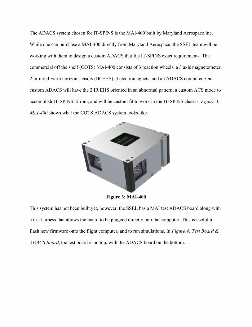
The ADACS system chosen for IT-SPINS is the MAI-400 built by Maryland Aerospace Inc.

While one can purchase a MAI-400 directly from Maryland Aerospace, the SSEL team will be

working with them to design a custom ADACS that fits IT-SPINS exact requirements. The

commercial off the shelf (COTS) MAI-400 consists of 3 reaction wheels, a 3 axis magnetometer,

2 infrared Earth horizon sensors (IR EHS), 3 electromagnets, and an ADACS computer. Our

custom ADACS will have the 2 IR EHS oriented in an abnormal pattern, a custom ACS mode to

accomplish IT-SPINS’ 2 rpm, and will be custom fit to work in the IT-SPINS chassis. Figure 3:

MAI-400 shows what the COTS ADACS system looks like.

Figure 3: MAI-400

This system has not been built yet, however, the SSEL has a MAI test ADACS board along with

a test harness that allows the board to be plugged directly into the computer. This is useful to

flash new firmware onto the flight computer, and to run simulations. In Figure 4: Test Board &

ADACS Board, the test board is on top, with the ADACS board on the bottom.

Figure 4: Test Board & ADACS Board

These are very expensive proprietary boards, so all electrostatic discharge (ESD) precautions

must be taken when dealing with them. These include wearing ESD preventative lab coats and

grounding bracelets that ground you to the table. To simulate day-to-day operations, the test and

ADACS board are connected to the computer. Then, as seen in Figure 5: Dynamic Simulator, a

dynamic simulator is run on the computer that simulates input data the board would see in space.

Figure 5: Dynamic Simulator

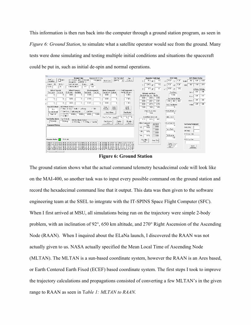
This information is then run back into the computer through a ground station program, as seen in

Figure 6: Ground Station, to simulate what a satellite operator would see from the ground. Many

tests were done simulating and testing multiple initial conditions and situations the spacecraft

could be put in, such as initial de-spin and normal operations.

Figure 6: Ground Station

The ground station shows what the actual command telemetry hexadecimal code will look like

on the MAI-400, so another task was to input every possible command on the ground station and

record the hexadecimal command line that it output. This data was then given to the software

engineering team at the SSEL to integrate with the IT-SPINS Space Flight Computer (SFC).

When I first arrived at MSU, all simulations being run on the trajectory were simple 2-body

problem, with an inclination of 92°, 650 km altitude, and 270° Right Ascension of the Ascending

Node (RAAN). When I inquired about the ELaNa launch, I discovered the RAAN was not

actually given to us. NASA actually specified the Mean Local Time of Ascending Node

(MLTAN). The MLTAN is a sun-based coordinate system, however the RAAN is an Ares based,

or Earth Centered Earth Fixed (ECEF) based coordinate system. The first steps I took to improve

the trajectory calculations and propagations consisted of converting a few MLTAN’s in the given

range to RAAN as seen in Table 1: MLTAN to RAAN.

MLTAN (hours) RAAN

1630 273°

1745 292°

1900 311°

Table 1: MLTAN to RAAN

As seen above, none of the given RAAN values are within the 270° previously used to propagate

the orbit. The second improvement I added to the trajectory propagation was adding a much

more complex propagation model. This model included aerodynamic drag, non-spherocity of the

Earth, gravity gradient torque, solar radiation pressure, and the pull of the masses of the Sun and

the Moon on the spacecraft. All of this combined to create a very complex and much more

accurate propagation model. Interestingly enough, this model predicts no eclipses for the first

month, with the first eclipse lasting 5 minutes on the 10th of November 2017. Another necessary

calculation that I did was the sun vector calculations. These calculations consisted of determining

the angle of each of the six sides of IT-SPINS with the Sun at any given time. These angles,

combined with the max power output of the solar panels on each side, can be used to calculate

the power budget of the satellite. A good way to visualize the orbit’s orientation related to the

sun is the 𝛽 angle. The 𝛽 angle is the angle between a vector normal to the orbital plane, and the

satellite’s sun vector. The 𝛽 angle can be calculated by taking the cross product of the position

and velocity vectors of the satellite with respect to (WRT) the Earth, and the dot product of the

Sun vector of the satellite and that perpendicular vector. Running this calculation through a

MATLAB script gives Figure 7: Sun Angle vs. Time.

Figure 7: Sun Angle vs. Time

The sections of this figure in green are when the satellite gets the most sunlight, versus the

sections in red when it gets the least sunlight.

Mission Concept 1

Another satellite mission I worked on is called Mission Concept 1. It’s a 6U Cube Sat

with a mission to detect optical signatures of atmospheric gravity waves (AGW), traveling

atmospheric disturbances (TAD), and traveling ionospheric disturbances (TID) against the limb

far ultraviolet (FUV) background. It is planned to launch in Early 2018 and has a non-circular

orbit. To complete its scientific mission, its perigee must be between 400-600 km altitude and its

apogee must be between 500-600 km altitude and must have an inclination greater than 65°. It

will have two attitude modes during its mission, one spinning very similar to IT-SPINS at 2 rpm,

and another one that involves simple nadir pointing. This mission is currently in the

concept/proposal phase. To properly prepare a preliminary power budget for Mission Concept 1,

I ran simulations of possible orbits within its scientific orbital parameters. From this I could

determine the best and worst case scenarios, as seen in Table 2: Mission Concept 1 Orbital

Analysis.

Orbital Element Effect on Sunlight Worst Case Best Case Correlation

RAAN Medium 225° 90° Sinusoidal

Inclination Large 50° 70° Linear (higher is better)

AOP Small 180° 315° Sinusoidal

Perigee Large 400 km 600 km Linear (higher is better)

Apogee Large 500 km 600 km Linear (higher is better)

Mission Concept 1 Orbital Analysis

Mission Concept 2

Another satellite mission I worked on is called Mission Concept 2. It’s a 6U Cube Sat

with a mission to take in-situ measurements of the O+ and H+ temperatures and the electron

temperature in the same volume. It is planned to launch in Summer 2019 and has a non-circular

orbit. To complete its scientific mission, its perigee must be between 400-500 km altitude and its

apogee must be greater than 800 km altitude. It must have an inclination greater than 50°. It will

have 1 attitude mode during its mission, ram-pointing, which means it will be facing its sensors

in the velocity direction. This mission is currently in the concept/proposal phase. To properly

prepare a preliminary power budget for Mission Concept 2, I ran simulations of possible orbits

within its scientific orbital parameters. From this I could determine the best and worst case

scenarios, as seen in Table 3: Mission Concept 2 Orbital Analysis.

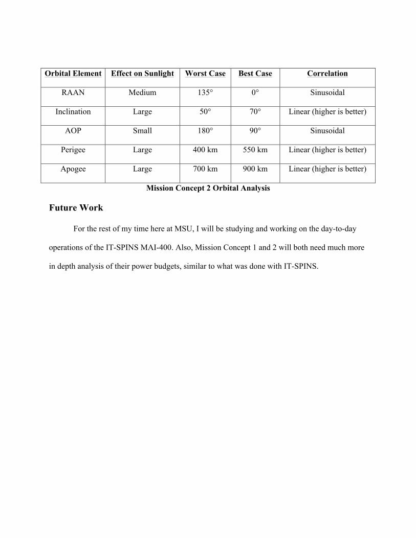
Orbital Element Effect on Sunlight Worst Case Best Case Correlation

RAAN Medium 135° 0° Sinusoidal

Inclination Large 50° 70° Linear (higher is better)

AOP Small 180° 90° Sinusoidal

Perigee Large 400 km 550 km Linear (higher is better)

Apogee Large 700 km 900 km Linear (higher is better)

Mission Concept 2 Orbital Analysis

Future Work

For the rest of my time here at MSU, I will be studying and working on the day-to-day

operations of the IT-SPINS MAI-400. Also, Mission Concept 1 and 2 will both need much more

in depth analysis of their power budgets, similar to what was done with IT-SPINS.