mse3 ch06 clouds - university of british columbia€¦ · 159 chapter 6 clouds 6 clouds have...

159

chapter 6

clouds

6 Clouds have immense beauty and variety. They show weather patterns on a global scale, as viewed by satellites. Yet they are

made of tiny droplets that fall gently through the air. Clouds can have richly complex fractal shapes, and a wide distribution of sizes. Clouds are named according to an international cloud classification scheme. Clouds form when air becomes saturated. Satu-ration can occur by adding water, by cooling, or by mixing; hence, Lagrangian water and heat budgets are useful. The buoyancy of the cloudy air and the static stability of the environment determine the vertical extent of the cloud. Fogs are clouds that touch the ground. Their lo-cation in the atmospheric boundary layer means that turbulent transport of heat and moisture from the underlying surface affects their formation, growth, and dissipation.

processes causing saturation

Clouds are saturated portions of the atmosphere where small water droplets or ice crystals have fall velocities so slow that they appear visibly suspend-ed in the air. Thus, to understand clouds we need to understand how air can become saturated.

cooling and Moisturizing Unsaturated air parcels can reach saturation by three processes: cooling, adding moisture, or mix-ing. The first two processes are shown in Fig. 6.1, where saturation is reached by either cooling until the temperature equals the dew point temperature, or adding moisture until the dew point tempera-ture is raised to the actual ambient temperature. The temperature change necessary to saturate an air parcel by cooling it is:

∆ = −T T Td (6.1)

Whether this condition is met can be determined by finding the actual temperature change based on the first law of thermodynamics (see the Heat chapter).

contents

Processes Causing Saturation 159Cooling and Moisturizing 159Mixing 160

Cloud Identification & Development 161Cumuliform 161Stratiform 162Stratocumulus 164Others 164

Clouds in unstable air aloft 164Clouds associated with mountains 165Clouds due to surface-induced turbulence 165Anthropogenic Clouds 166

Cloud Organization 167

Cloud Classification 168Genera 168Species 168Varieties 169Supplementary Features 169Accessory Clouds 169

Sky Cover (Cloud Amount) 170

Cloud Sizes 170

Fractal Cloud Shapes 171Fractal Dimension 171Measuring Fractal Dimension 172

Fog 173Types 173Idealized Fog Models 173

Advection Fog 173Radiation Fog 175Dissipation of Well-Mixed (Radiation and

Advection) Fogs 176

Summary 178Threads 178

Exercises 179Numerical Problems 179Understanding & Critical Evaluation 181Web Enhanced Questions 183Synthesis Questions 183

Copyright © 2011, 2015 by Roland Stull. Meteorology for Scientists and Engineers, 3rd Ed.

“Meteorology for Scientists and Engineers, 3rd Edi-tion” by Roland Stull is licensed under a Creative Commons Attribution-NonCommercial-ShareAlike

4.0 International License. To view a copy of the license, visit http://creativecommons.org/licenses/by-nc-sa/4.0/ . This work is available at http://www.eos.ubc.ca/books/Practical_Meteorology/ .

160 ChAPTEr 6 ClOUDS

The moisture addition necessary to reach satura-tion is ∆ = −r r rs (6.2)

Whether this condition is met can be determined by using the moisture budget to find the actual humid-ity change (see the Moisture chapter). In the real atmosphere, sometimes both cooling and moisturizing happen simultaneously. Sche-matically, this would correspond to an arrow from parcel A diagonally to the saturation line of Fig. 6.1. Clouds usually form by adiabatic cooling of ris-ing air. Air can be rising due to its own buoyancy (making cumuliform clouds), or can be forced up over hills or frontal boundaries (making stratiform clouds). Once formed, infrared radiation from cloud top can cause additional cooling to help maintain the cloud.

Mixing Mixing of two unsaturated parcels can result in a saturated mixture, as shown in Fig. 6.2. Jet contrails and your breath on a cold winter day are examples of clouds that form by the mixing process. Mixing essentially occurs along a straight line in this graph connecting the thermodynamic states of the two original air parcels. However, the satura-tion line (given by the Clausius-Clapeyron equation) is curved, so a mixture can be saturated even if the original parcels are not. Let mB and mC be the original masses of air in parcels B and C, respectively. The mass of the mix-ture (parcel X) is :

m m mX B C= + (6.3)

Solved Example Air at sea level has a temperature of 20°C and a mixing ratio of 5 g/kg. How much cooling OR mois-turizing is necessary to reach saturation?

SolutionGiven: T = 20°C, r = 5 g/kgFind: ∆T = ? °C, ∆r = ? g/kg.

Use Table 4-1 because it applies for sea level. Other-wise, solve equations or use a thermo diagram.At T = 20°C, the table gives rs = 14.91 g/kg .At r = 5 g/kg, the table gives Td = 4 °C .

Use eq. (6.1): ∆T = 4 – 20 = –16°C needed.Use eq. (6.2): ∆r = 14.91 – 5 = 9.9 g/kg needed.

Check: Units OK. Physics OK.Discussion: This air parcel is fairly dry. Much cool-ing or moisturizing is needed.

Figure 6.1Unsaturated air parcel “A” can become saturated by the addi-tion of moisture, or by cooling. The curved line is the saturation vapor pressure from the Moisture chapter.

Figure 6.2Mixing of two unsaturated air parcels B and C, which occurs along a straight line (dashed), can cause a saturated mixture X. The curved line is the saturation vapor pressure from the Mois-ture chapter.

r. STUll • METEOrOlOGy FOr SCIENTISTS AND ENGINEErS 161

The temperature and vapor pressure of the mix-ture are the weighted averages of the corresponding values in the original parcels:

Tm T m T

mXB B C C

X=

⋅ + ⋅ (6.4)

em e m e

mXB B C C

X=

⋅ + ⋅ (6.5)

Specific humidity or mixing ratio can be used in place of vapor pressure in eq. (6.5). Instead of using the actual masses of the air par-cels in eqs. (6.3) to (6.5), you can use the relative por-tions that mix. For example, if the mixture consists of 3 parts B and 2 parts C, then you can use mB = 3 and mC = 2 in the equations above.

cloud identification &

developMent

You can easily find beautiful photos of all the clouds mentioned below by pointing your web-browser search engine at “cloud classification”, “cloud identification”, “cloud types”, or “Interna-tional Cloud Atlas”. You can also use web search engines to find images of any named cloud. To help keep the cost of this book reasonable, I do not in-clude any cloud photos.

cumuliform Cumuliform clouds form vertically in up-drafts, and look like fluffy puffs of cotton, cauli-flower, rising castle turrets, or in extreme instabil-ity as anvil-topped thunderstorms that look like big mushrooms. These clouds have diameters roughly equal to the height of their cloud tops above ground (Fig. 6.3). Thicker clouds look darker when viewed from underneath, but when viewed from the side, the cloud sides and top are often bright white dur-ing daytime. The individual clouds are often sur-rounded by clearer air, where there is compensating subsidence (downdrafts). Cumulus clouds frequently have cloud bases within 1 or 2 km of the ground (in the boundary lay-er). But their cloud tops can be anywhere within the troposphere (or lower stratosphere for the strongest thunderstorms). Cumuliform clouds are named by their thick-ness, not by the height of their base (Fig. 6.3). Start-ing from the thinnest (with lowest tops), the clouds are cumulus humilis (fair-weather cumulus),

Figure 6.3Cloud identification: cumuliform. These are lumpy clouds caused by convection (updrafts) from the surface.

Solved Example Suppose that the state of parcel B is T = 30°C with e = 3.4 kPa, while parcel C is T = –4°C with e = 0.2 kPa. Both parcels are at P = 100 kPa. If each parcel contains 1 kg of air, then what is the state of the mixture? Will the mixture be saturated?

SolutionGiven: B has T = 30°C, e = 3.4 kPa, P = 100 kPa C has T = –4°C, e = 0.2 kPa, P = 100 kPaFind: T = ? °C and e = ? kPa for mixture (at X).

Use eq. (6.3): mX = 1 + 1 = 2 kgUse eq. (6.4): TX = [(1kg)·(30°C) + (1kg)·(–4°C)]/(2kg) = 13°C.Use eq. (6.5): eX = [(1kg)·(3.4 kPa) + (1kg)·(0.2 kPa)]/(2kg) = 1.8 kPaP hasn’t changed. P = 100 kPa.

Check: Units OK. Physics OK.Discussion: At T = 13°C, Table 4-1 gives es = 1.5 kPa. Thus, the mixture is saturated because its vapor pres-sure exceeds the saturation vapor pressure. This mix-ture would be cloudy/foggy.


cumulus mediocris, cumulus congestus (tow-ering cumulus), and cumulonimbus (thunder-storms). Cumuliform clouds develop in statically un-stable air. The unstable air tries to turbulently stabilize itself by creating convective updrafts and downdrafts. Cumuliform clouds can form in the tops of warm updrafts (thermals) if sufficient mois-ture is present. Hence, cumulus clouds are convec-tive clouds. These clouds are dynamically active in the sense that their own internal buoyancy-forces (associated with latent heat release) enhance and support the convection and their vertical growth. If the air is continually destabilized by some ex-ternal forcing, then the convection persists. Some favored places for destabilization and small to me-dium cumulus clouds are:

• behind cold fronts, • on mostly clear days when sunshine warms the ground more than the overlying air,• over urban and industrial centers that are warmer than the surrounding rural areas, • when cold air blows over a warmer ocean or lake. Cold fronts trigger deep cumuliform clouds (thunderstorms) along the front, because the ad-vancing cold air strongly pushes up the warmer air ahead of it, destabilizing the atmosphere and trig-gering the updrafts (see Thunderstorm chapters). Also mountains can trigger all sizes of cumulus clouds including thunderstorms. One mechanism is orographic lift, when horizontal winds hit the mountains and are forced up. Another mechanism is anabatic circulation, where mountain slopes heated by the sun tend to organize the updrafts along the mountain tops (see Local Winds chapter). Once triggered, cumulus clouds can continue to grow and evolve somewhat independently of the initial trigger. For example, orographically-trig-gered thunderstorms can persist as they are blown away from the mountain. On a thermo diagram, cloud top is where the buoyant cloud parcel crosses the environmental sounding, and loses its positive buoyancy (Fig. 6.4). Cloud base is the lifting condensation level (LCL).

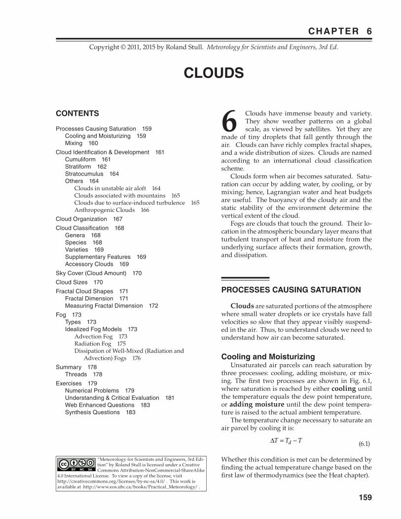
stratiform Stratiform clouds are horizontally layered clouds that look like sheets or blankets covering wide areas (Fig. 6.5). Clouds ahead of warm fronts are typically stratiform, including: cirrus, cirro-stratus, cirrocumulus, altostratus, altocumu-lus, stratus, and nimbostratus. Layered clouds are often grouped (high, middle, low) by their relative altitude or level within the

Solved Example Use the sounding in the solved example on the same page as the start of the “Parcel vs. Environment” section of the Stability chapter. Where is cloud base and top for an air parcel rising from the surface?

SolutionGiven: sounding from the Stability chapter.Find: Pbase = ? kPa, Ptop = ? kPa

First, plot the sounding on a large thermo diagram from the Stability chapter. Then conceptually lift a parcel dry adiabatically from the surface until it cross-es the isohume from the surface. That LCL is at Pbase = 80 kPa. However, the parcel never gets there. It hits the en-vironment below the LCL, at roughly P = 83 kPa. Ne-glecting any inertial overshoot of the parcel, it would have zero buoyancy and stop rising 3 kPa below the LCL. Thus, there is no cloud from rising surface air.

Check: Units OK. Physics OK.Discussion: This was a trick question. Also, the pres-ence of mid-level stratiform clouds is irrelevant.

Figure 6.4Characteristic sounding for cumulus humilis and altocumulus castellanus clouds. Solid thick black line is temperature; dashed black line is dew point; LCL = lifting condensation level. The cumulus humilis clouds form in thermals of warm air rising from the Earth’s surface. The altocumulus castellanus clouds are a special stratiform cloud (discussed later in this chapter) that are not associated with thermals rising from the Earth’s surface.


troposphere. However, troposphere thickness and tropopause height vary considerably with latitude (high near the equator, and low near the poles, see Table 6-1). It also varies with season (high during summer, low during winter). Thus, low, middle and high clouds can have a range of altitudes. Table 6-1 lists cloud levels and their altitudes as defined by World Meteorologi-cal Organization (WMO). These heights are only approximate, as you can see from the overlapping values in the table. High, layered clouds have the prefix “cirro” or “cirrus”. The cirrus and cirrostratus are often wispy or have diffuse boundaries, and indicate that the cloud particles are made of ice crystals. In the right conditions, these ice-crystal clouds can cause beau-tiful halos around the sun or moon. See the last chapter for a discussion of atmospheric optics. Mid-level, layered clouds have the prefix “alto”. These and the lower clouds usually contain liquid water droplets, although some ice crystals can also be present. In the right conditions (relatively small uniformly sized drops, and a thin cloud) you can see an optical effect called corona. Corona appears as a large disk of white light centered on the sun or moon (still visible through the thin cloud). Colored fringes surround the perimeter of the white disk (see the Optics chapter). Cirrostratus and altostratus are particularly smooth looking, which implies little or no turbu-lence within them. Cirrocumulus and altocumulus are layers of lumpy clouds, but the lumps are small and the edges are often sharply defined, suggesting that they are predominantly composed of liquid wa-ter droplets. We infer from these small sizes that the turbulent eddies causing these lumps are locally generated within the cloud layer, and are not associ-ated with updrafts from the ground. Stratus is a thick, smooth, cloud layer at low altitudes, but this type of cloud is not turbulently coupled with the underlying surface. Nimbostratus clouds are thick enough to allow drizzle or rain to form and fall out. The prefix “nimbo” or suffix “nimbus” origi-nally designated a precipitating cloud, but such a meaning is no longer prescribed in the internation-al cloud atlas. Nimbostratus usually have light to moderate rain or snow over large horizontal areas, while cumulonimbus (thunderstorm) clouds have heavy rain (or snow in winter) and sometimes hail in small areas or along narrow paths on the ground called swaths (e.g., hail swaths or snow swaths). Stratiform clouds form in statically stable air. These are dynamically passive, in the sense that buoyant forces suppress their vertical growth. These clouds exist only while some external process causes lifting to overcome the buoyancy.

Figure 6.5Cloud identification: stratiform. Layered clouds caused by nearly horizontal advection of moisture by winds. “Mix” indi-cates a mixture of liquid and solid water particles. Heights “z” are only approximate — see Table 6–1 for actual ranges.

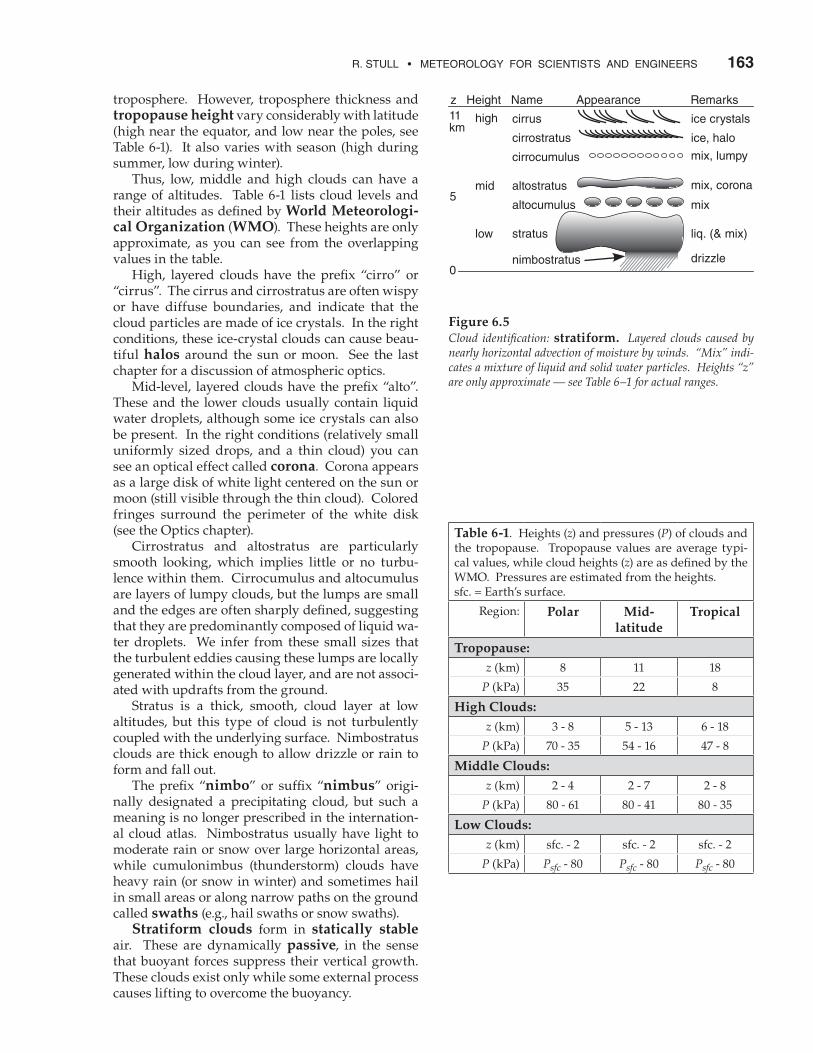
Table 6-1. Heights (z) and pressures (P) of clouds and the tropopause. Tropopause values are average typi-cal values, while cloud heights (z) are as defined by the WMO. Pressures are estimated from the heights. sfc. = Earth’s surface.

Region: Polar Mid-latitude

Tropical

Tropopause:z (km) 8 11 18

P (kPa) 35 22 8

High Clouds:z (km) 3 - 8 5 - 13 6 - 18

P (kPa) 70 - 35 54 - 16 47 - 8

Middle Clouds:z (km) 2 - 4 2 - 7 2 - 8

P (kPa) 80 - 61 80 - 41 80 - 35

Low Clouds:z (km) sfc. - 2 sfc. - 2 sfc. - 2

P (kPa) Psfc - 80 Psfc - 80 Psfc - 80


stratocumulus Stratocumulus clouds are low layers of lumpy clouds, often covering 5/8 or more of the sky (Fig. 6.3). They are somewhat different from either ac-tive and passive clouds. Unlike passive clouds, they can be formed by updrafts by air rising from near the surface. Unlike active clouds, these updrafts are sometimes not caused by buoyancy, but can be caused by turbulence generated by wind shear. The larger eddy circulations in the turbulence can lift air parcels from the ground up to the LCL, allowing the clouds to form. Unlike stratus clouds, stratocumulus clouds are turbulently coupled with the underlying surface, and their cloud bases can be estimated us-ing the LCL for near-surface air. In the real atmosphere, both buoyancy and shear often contribute to the updrafts into the base of stratocumulus clouds. Also, IR radiation emit-ted upward from cloud top can cool the cloud top, creating cool air parcels that sink as upside-down thermals (i.e., convection driven by cooling from the top, instead of by heating from below). The re-sulting turbulent circulations can contribute to the lumpiness of the stratocumulus deck (cloud layers are sometimes called cloud decks).

others There are many beautiful and unusual clouds that do not fit well into the cumuliform and stratiform categories. A few are discussed here: castellanus, lenticular, cap, rotor, banner, contrails, fumulus, bil-low clouds, pileus, and fractus. Again, you can find pictures of these using your web browser. Other clouds associated with thunderstorms are described in the Thunderstorm chapters. These in-clude funnel, wall, mammatus, arc, shelf, flanking line, beaver tail, and anvil.

Clouds in unstable air aloft Two types of clouds can form in layers of stati-cally or dynamically unstable air aloft: castellanus and billow clouds. Castellanus clouds are distinctive because their diameters are small compared to their height above ground, making them look like castle turrets (Fig. 6.4). They can form in layers of statically unstable air aloft. These layers are forced by differential advection; namely, by wind blowing in air of dif-ferent temperatures from different directions at dif-ferent heights. For castellanus clouds, differential advection creates a layer of relatively warm air un-der colder air, which is statically unstable. If these form just above the top of the boundary layer, they are called cumulus castellanus. When slightly higher, in the middle of the troposphere, they are called altocumulus castellanus. Alto-

For most stratiform clouds, the external forcing is horizontal advection (movement by the mean wind), where humid air is blown up a gently-in-clined warm-frontal surface from moisture sources hundreds to thousands of kilometers away. This process is illustrated in Fig. 5.20. Let the cir-cle in that figure represent a humid air parcel with potential temperature 290 K. If a southerly wind were tending to blow the parcel toward the pole, the parcel would follow the 290 K isentrope like a train on tracks, and would ride up over the colder surface air in the polar portion of the domain. The gentle rise of air along the isentropic surface creates suf-ficient cooling to cause the condensation. Stratiform clouds can be inferred from sound-ings (Fig. 6.6), in the layers above the boundary layer where environmental temperature and dew point are equal (i.e., where the sounding lines touch). Due to inaccuracies in some of the sounding instruments, sometimes the T and Td lines become close and par-allel over a layer without actually touching. You can infer that these are also stratiform cloud layers. All of the stratiform clouds listed above are not convectively coupled with the ground directly underneath them. Hence, their cloud base cannot be calculated using the LCL for air directly under them. In spite of their lumpiness, cirrocumulus and altocumulus are formed primarily by advection, and are passive layer (i.e., stratiform) clouds. Do not let the suffix “cumulus” in those cloud names fool you. In North America the nimbostratus clouds of-ten have low bases, and are considered to be a low cloud. However, as we will see in the international cloud classification section, nimbostratus clouds are traditionally listed a mid-level clouds. In this book, we will treat nimbostratus as stratiform rain clouds with low cloud base.

Figure 6.6Characteristic sounding for stratiform clouds.


cumulus castellanus are sometimes precursors to thunderstorms (because they indicate an unstable mid-troposphere), and are a useful clue for storm chasers. Billow clouds (discussed in the Stability chap-ter) are a layer of many parallel, horizontal lines of cloud that form in the crests of Kelvin-Helmholtz (K-H) waves (Fig. 5.17). They indicate a layer of tur-bulence aloft caused by wind shear and dynamic in-stability. Pilots avoid these turbulent layers. When similar turbulent layers form with insufficient mois-ture to be visible as billow clouds, the result is a lay-er of clear-air turbulence (CAT), which pilots also try to avoid. Sometimes instead of a layer of billows, there will be only a narrow band of breaking wave clouds known as K-H wave clouds.

Clouds associated with mountains In mountainous regions with sufficient humidi-ty, you can observe lenticular, cap, rotor, and banner clouds. The Local Winds chapter discusses others. Lenticular clouds have smooth, distinctive lens or almond shapes when viewed from the side, and they are centered on the mountain top or on the crest of the lee wave (Fig. 6.7). They are also known as mountain-wave clouds, and are dynamically passive clouds that form in hilly regions. If a len-ticular cloud forms directly over a mountain, it is sometimes called a cap cloud. Cap clouds are caused by updrafts forced when statically-stable air, blown horizontally by the wind, hits sloping terrain or mountains. Lenticular clouds can form in the crest of vertical oscillations in the air called moun-tain waves that form downwind of mountains. They are a most unusual cloud, because the cloud remains relatively stationary while the air blows through it. Hence, they are known as stand-ing lenticular. The uniformity of droplet sizes in lenticular clouds create beautiful optical phenom-ena called iridescence when the sun appears close to the cloud edge. See the Local Winds chapter for mountain wave details, and the Optics chapter for more on atmospheric optics. Rotor clouds are violently turbulent balls or bands of ragged cloud that rapidly rotate along a horizontal axis (Fig. 6.7). They form relatively close to the ground under the crests of mountain waves (e.g., under standing lenticular clouds), but much closer to the ground. Pilots flying near the ground downwind of mountains during windy conditions should watch out for, and avoid, these hazardous clouds, because they indicate severe turbulence. The banner cloud is a very turbulent stream-er attached to the mountain top that extends like a banner or flag downwind (Fig. 6.7). It forms on the lee side at the very top of high, sharply pointed,

mountain peaks during strong winds. As the wind separates to flow around the mountain, low pressure forms to the lee of the mountain peak, and counter-rotating vortices form on each side of the mountain. These work together to draw air upward along the lee slope, causing cooling and condensation. These strong turbulent winds can also pick up previously fallen ice particles from snow fields on the mountain surface, creating a snow banner that looks similar to the banner cloud.

Clouds due to surface-induced turbulence The most obvious clouds formed due to surface-induced turbulence are the cumuliform (convec-tive) clouds already discussed. However, there are two others that we haven’t covered yet: pileus and fractus. The pileus cloud looks like a thin hat just above, or scarf around, the top of the rising cumulus clouds (Fig. 6.8). It forms in mid-tropospheric humid (near-ly saturated) layers of statically stable air that are forced upward above the tops of rapidly rising cu-mulus congestus clouds (hence, the indirect influ-ence from surface heating). These are very short lived, because the cloud towers quickly rise through the pileus and engulf them. Fractus clouds are ragged, shredded, often low-altitude clouds that form and dissipate quickly (Fig. 6.8). They can form during windy conditions in the turbulent, boundary-layer air near rain showers, under the normal nimbostratus or cumulonimbus cloud base. These clouds do not need mountains to form, but are often found along the sides of moun-tains during rainy weather. The falling rain from the cloud above adds moisture to the air, and the up-draft portions of turbulent eddies provide the lifting to reach condensation. Sometimes fractus clouds form in non-rainy con-ditions, when there is both strong winds and strong

Figure 6.7Some clouds caused by mountains, during strong winds.


solar heating. In this case, the rising thermals lift air to its LCL, while the intense turbulence in the wind shear shreds and tears apart the resulting cumulus clouds to make cumulus fractus.

Anthropogenic Clouds The next two clouds are anthropogenic (man-made). These are contrails and fumulus. Fumulus is a contraction for “fume cumulus”. They form in the tops of thermal plumes rising from cooling towers, forest fires, or smokestacks (Fig. 6.8). Modern air-quality regulations often require that industries scrub the pollutants out of their stack gas-ses by first passing the gas through a scrubber (i.e., a water shower). Although the resulting effluent much is less polluted, it usually contains more wa-ter vapor, and thus can cause beautiful white clouds of water droplets within the rising exhaust plume. Similarly, cooling towers do their job by evaporating water to help cool an industrial process, while forest fires produce water vapor and smoke as combustion products when wood burns. Contrail is a contraction for “condensation trail”, and is the straight, long, narrow, horizontal pair of clouds left behind a high-altitude aircraft (Fig. 6.8). Aircraft fuel is a hydrocarbon, so its combustion in a jet engine produces carbon dioxide and water vapor. Contrails form when water vapor in the exhaust of high-altitude aircraft mixes with the cold environ-mental air at that altitude (see mixing subsection earlier in this chapter). If this cold air is already nearly saturated, then the additional moisture from the jet engine is sufficient to form a cloud. On drier days aloft, the same jet aircraft would produce no visible contrails. Regardless of the number of engines on the air-craft, the exhaust tends to be quickly entrained into the horizontal wing-tip vortices that trail behind the left and right wing tips of the aircraft. Hence, jet contrails often appear initially as a pair of closely-spaced, horizontal parallel lines of cloud. Further behind the aircraft, environmental wind shears of-ten bend and distort the contrails. Turbulence breaks apart the contrail, causes the two clouds to merge into one contrail, and eventually mixes enough dry ambient air to cause the contrail to evaporate and disappear. Contrails might have a small effect on the global-climate heat budget by reflecting some of the sun-light. Contrails are a boon to meteorologists be-cause they are a clue that environmental moisture is increasing aloft, which might be the first indication of an approaching warm front. They are a bane to military pilots who would rather not have the enemy see a big line in the sky pointing to their aircraft.

Figure 6.8Other clouds.

focus • strato- & Mesospheric clouds

Although almost all our clouds occur in the tro-posphere, sometimes higher-altitude thin stratiform (cirrus-like) clouds can be seen. They occur poleward of 50° latitude during situations when the upper at-mosphere temperatures are exceptionally cold. These clouds are so diffuse and faint that you can-not see them by eye during daytime. These clouds are visible at night for many minutes near the end of evening twilight or near the beginning of morn-ing twilight. The reason these clouds are visible is because they are high enough to still be illuminated by the sun, even when lower clouds are in the Earth’s shadow. Highest are noctilucent clouds, in the meso-sphere at heights of about 85 km. They are made of tiny H2O ice crystals (size ≈ 10 nm), and are nucle-ated by meteorite dust. Noctilucent clouds are polar mesospheric clouds (PMC), and found near the polar mesopause during summer. Lower (20 to 30 km altitude) are polar strato-spheric clouds (PSC). At air temperatures below –78°C, nitric acid trihydrate (NAT-clouds) can con-dense into particles. Also forming at those tempera-tures can be particles made of a supersaturated mix-ture of water, sulphuric acid, and nitric acid (causing STS clouds). For temperatures colder than –86°C in the strato-sphere, pure H2O ice crystals can form, creating PSCs called nacreous clouds. They are also known as mother-of-pearl clouds because they exhibit beautiful iridescent fringes when illuminated by the sun. These stratospheric clouds form over mountains, due to mountain waves that propagate from the tropo-sphere into the stratosphere, and amplify there in the lower-density air. They can also form over extremely

intense tropospheric high-pressure regions.


cloud organization

Clouds frequently become organized into pat-terns during stormy weather. This organization is discussed in the chapters on Fronts, Midlatitude Cy-clones, Thunderstorms, and Hurricanes. Also, some-times large-scale processes can organize clouds even during periods of fair weather, as discussed here. Cloud streets or cloud lines are rows of fair-weather cumulus-humilis clouds (Fig. 6.9) that are roughly parallel with the mean wind direction. They form over warm land in the boundary layer on sunny days, and over water day or night when cold air advects over warmer water. Light to moderate winds in the convective boundary layer cause hori-zontal roll vortices, which are very weak counter-rotating circulations with axes nearly parallel with the mean wind direction. These weak circulations sweep rising cloud-topped thermals into rows with horizontal spacing of roughly twice the boundary-layer depth (order of 1 km).

Mesoscale cellular convection (MCC) can also form in the boundary layer, but with a much larger horizontal scale (order of 5 to 50 times the boundary layer depth; namely, 10 to 100 km in di-ameter). These are so large that the organization is not apparent to observers on the ground, but is read-ily visible in satellite images. Open cells consist of a honeycomb or rings of cloud-topped updrafts around large clear regions (Fig. 6.9). Closed cells are the opposite — a honeycomb of clear-air rings around cloud clusters. Cloud streets changing into MCC often form when cold continental air flows over a warmer ocean. [WARNING: Abbreviation MCC is also used for Mesoscale Convective Complex, which is a cluster of deep thunderstorms.]

on doing science • cargo cult science

“In the South Seas there is a cargo cult of people. During the war they saw airplanes land with lots of good materials, and they want the same thing to hap-pen now. So they’ve arranged to make things like runways, to put fires along the sides of the runways, to make a wooden hut for a man to sit in, with two wooden pieces on his head like headphones and bars of bamboo sticking out like antennas – he’s the control-ler – and they wait for the airplanes to land. They’re doing everything right. The form is perfect. It looks exactly the way it looked before. But it doesn’t work. No airplanes land. So I call these things cargo cult sci-ence, because they follow the apparent precepts and forms of scientific investigation, but they’re missing something essential, because the planes don’t land.” “Now it behooves me, of course, to tell you what they’re missing. ... It’s a kind of scientific integrity, a principle of scientific thought that corresponds to a kind of utter honesty... For example, if you’re doing an experiment, you should report everything that you think might make it invalid – not only what you think is right about it: other causes that could pos-sibly explain your results; and things you thought of that you’ve eliminated by some other experiment, and how they worked – to make sure the other fellow can tell they have been eliminated.” “Details that could throw doubt on your interpre-tation must be given, if you know them. You must do the best you can – if you know anything at all wrong, or possibly wrong – to explain it. If you make a theory, ... then you must also put down all the facts that dis-agree with it, as well as those that agree with it. There is also a more subtle problem. When you have put a lot of ideas together to make an elaborate theory, you want to make sure when explaining what it fits, that those things it fits are not just the things that gave you the idea for the theory; but that the finished theory makes something else come out right, in addition.” “In summary, the idea is to try to give all the infor-mation to help others to judge the value of your con-tribution; not just the information that leads to judge-ment in one particular direction or another.” – Richard P. Feynman, 1985: “Surely You’re Joking, Mr. Feynman!”. Adventures of a Curious Character. Ban-tam. 322pp.

Figure 6.9Organized boundary-layer clouds, such as are seen in a satellite image. Grey = clouds.

science graffito

“Science is the belief in the ignorance of experts.” – Richard Feynman.


species Subdividing the genera are cloud species. Table 6-3 lists the official WMO species. Species can ac-count for:• forms (clouds in banks, veils, sheets, layers, etc.)• dimensions (horizontal or vertical extent)• internal structure (ice crystals, water droplets, etc.)• likely formation process (orographic lift, etc.)

Species are also mutually exclusive. An exam-ple of a cloud genus with specie is “Altocumulus castellanus (Ac cas)”, which is a layer of mid-level lumpy clouds that look like castle turrets.

Table 6-3. WMO cloud species. (Ab. = abbreviation)

Specie Ab Description

calvus calthe top of a deep Cu or Cb that is starting to become fuzzy, but no cirrus (ice) anvil yet

capillatus capCb having well defined streaky cirrus (ice) anvil

castellanus cas

small turrets looking like a crenellated castle. Turret height > diameter. Can apply to Ci, Cc, Ac, Sc.

congestus con

very deep Cu filling most of tro-posphere, but still having crisp cauliflower top (i.e., no ice an-vil). Often called Towering Cu (TCU).

fibratus fibnearly straight filaments of Ci or Cs.

floccus flo

small tufts (lumps) of clouds, often with virga (evaporating precip.) falling from each tuft. Applies to Ci, Cc, Ac, Sc.

fractus frashredded, ragged, irregular, torn by winds. Can apply to Cu and St.

humilis humCu of small vertical extent. Small flat lumps.

lenticularis len

having lens or almond cross section, often called mountain wave clouds. Applies to Cc, Ac, Sc.

mediocris med medium size Cu

nebulosus nebCs or St with veil or layer show-ing no distinct details

spissatus spi thick Ci that looks grey.

stratiformis strspreading out into sheets or horizontal layers. Applies to Ac, Sc, Cc.

uncinus unc hook or comma shaped Ci

cloud classification

Cloud morphology is the study and classifica-tion of cloud shapes. The classification method in-troduced in 1803 by Luke Howard is still used today, as approved by the World Meteorology Organiza-tion (WMO). WMO publishes an International Cloud Atlas with photos to help you identify clouds. As mentioned, you can easily find similar photos for free by point-ing your web search engine at “cloud classification”, “cloud identification”, “cloud types”, or “Internation-al Cloud Atlas”. The categories and subcategories of clouds are broken into: • genera - main characteristics of clouds • species - peculiarities in shape & structure • varieties - arrangement and transparency • supplementary features and accessory clouds - attached to other (mother) clouds • mother clouds - clouds with attachments • meteors - precipitation (ice, water, or mixed)Most important are the genera.

genera The ten cloud genera are listed in Table 6-2, along with their official abbreviations and symbols as drawn on weather maps. These genera are mutu-ally exclusive; namely, one cloud cannot have two genera. However, often the sky can have different genera of clouds adjacent to, or stacked above, each other.

Table 6-2. Cloud genera.

GenusAbbre-viation

WMOSymbol

USASymbol

cirrus Ci

cirrostratus Cs

cirrocumulus Cc

altostratus As

altocumulus Ac

nimbostratus Ns

stratus St

stratocumulus Sc

cumulus Cu

cumulonimbus Cb


varieties Genera and species are further subdivided into varieties (Table 6-4), based on:• transparency (sun or moon visible through cloud)• arrangement of visible elementsThese varieties are NOT mutually exclusive (except for translucidus and opacus), so you can append as many varieties to a cloud identification that apply. For example, “cumulonimbus capillatus translucidus undulatus” (Cb cap tr un).

Table 6-4. WMO cloud varieties.

Variety Ab. Description

duplicatus dusuperimposed cloud patches at slightly different levels. Applies to Ci, Cs, Ac, As, Sc.

intortus inCi with tangled, woven, or ir-regularly curved filaments

lacunosus lahoneycomb, chessboard, or reg-ular arrangement of clouds and holes. Applies to Cc, Ac, and Sc.

opacus optoo thick for the sun or moon to shine through. Applies to Ac, As, Sc, St.

perlucidus pea layer of clouds with small holes between elements. Ap-plies to Ac, Sc.

radiatus ra

very long parallel bands of clouds that, due to perspective, appear to converge at a point on the horizon. Applies to Ci, Ac, As, Sc, and Cu.

translucidus tr

layer or patch of clouds through which sun or moon is somewhat visible. Applies to Ac, As, Sc, St.

undulatus uncloud layers or patches showing waves or undulations. Applies to Cc, Cs, Ac, As, Sc, St.

vertebratus veCi streaks arranged like a skel-eton with vertebrae and ribs, or fish bones.

supplementary featuresTable 6-5. WMO cloud supplementary features, and the mother clouds to which they are attached. (Ab. = abbreviation.)

Feature Ab. Description

arcus arc

a dense horizontal roll cloud, close to the ground, along and above the leading edge of Cb gust-front outflows. Usually at-tached to the Cb, but can sepa-rate from it as the gust front spreads. Often has an arch shape when viewed from un-derneath, and a curved or arc shape in satellite photos.

incus inc

the upper portion of a Cb, spread out into an (ice) anvil with smooth, fibrous or striated appearance.

mamma mam

hanging protuberances of pouch-like appearance. Mammatus clouds are often found on the underside of Cb anvil clouds.

praecipitatio pra

precipitation falling from a cloud and reaching the ground. Mother clouds can be As, Ns, Sc, St, Cu, Cb.

tuba tub

a cloud column or funnel cloud protruding from a cloud base, and indicating an intense vor-tex. Usually attached to Cb, but sometimes to Cu.

virga vir

visible precipitation trails that evaporate before reaching the ground. They can hang from Ac, Cu, Ns or Cb clouds.

accessory clouds Smaller features attached to other clouds.

Table 6-6. WMO accessory clouds, and the mother clouds to which they are attached. (Ab.=abbreviation.)

Name Ab. Description

pannus pan

ragged shreds, sometimes in a con-tinuous layer, below a mother cloud and sometimes attached to it. Mother clouds can be As, Ns, Cu, Cb.

pileus pil

a smooth thin cap, hood, or scarf above, or attached to, the top of rapidly rising cumulus towers. Very transient, because the mother cloud quickly rises through and engulfs it. Mother clouds are Cu con or Cb.

velum vela thin cloud veil or sheet of large hori-zontal extent above or attached to Cu or Cb, which often penetrate it.


sky cover (cloud aMount) The fraction of the sky (celestial dome) covered by cloud is called sky cover, cloud cover, or cloud amount. It is measured in eights (oktas) according to the World Meteorological Organization. Table 6-7 gives the definitions for different cloud amounts, the associated symbol for weather maps, and the ab-breviation for aviation weather reports (METAR). Sometimes the sky is obscured, meaning that there might be clouds but the observer on the ground cannot see them. Obscurations (and their abbrevia-tions) include: mist [BR; horizontal visibilities ≥ 1 km (i.e., ≥ 5/8 of a statute mile)], fog [FG; visibilities < 1 km (i.e., < 5/8 statute mile)], smoke (FU), vol-canic ash (VA), sand (SA), haze (HZ), spray (PY), widespread dust (DU). For aviation, the altitude of cloud base for the lowest cloud with coverage ≥ 5 oktas (i.e., lowest bro-ken or overcast clouds) is considered the ceiling. For obscurations, the vertical visibility (VV) dis-tance is reported as a ceiling instead.

cloud sizes

Cumuliform clouds typically have diameters roughly equal to their depths, as mentioned previ-ously. For example, a fair weather cumulus cloud typically averages about 1 km in size, while a thun-derstorm might be 10 km. Not all clouds are created equal. At any given time the sky contains a spectrum of cloud sizes that has a lognormal distribution (Fig. 6.10, eq. 6.6)

f XXX S

X LSX

X

X( ) exp .

ln( / )= ∆π ⋅ ⋅

⋅ − ⋅

20 5

2

(6.6)

Solved Example Use a spreadsheet to find and plot the fraction of clouds ranging from X = 50 to 4950 m width, given ∆X = 100 m, SX =0.5, and LX = 1000 m.

SolutionGiven: ∆X = 100 m, SX =0.5, LX = 1000 m.Find: f(X)= ?

Solve eq. (6.6) on a spreadsheet. The result is: X (m) f(X) 50 2.558x10–8

150 0.0004 250 0.0068 350 0.0252 450 0.0495 550 0.0710 etc. etc. Sum of all f = 0.999

Check: Units OK. Physics almost OK, but the sum of all f should equal 1.0, representing 100% of the clouds. The reason for the error is that we should have con-sidered clouds even larger than 4950 m, because of the tail on the right of the distribution. Also smaller ∆X would help.Discussion: Although the dominant cloud width is about 800 m for this example, the long tail on the right of the distribution shows that there are also a small number of large-diameter clouds. Figure 6.10

Lognormal distribution of cloud sizes.

Table 6-7. Sky cover. Oktas= eighths of sky covered.

SkyCover(oktas)

Sym-bol

Name Abbr.Sky

Cover(tenths)

0Sky

Clear SKC 0

1 Few*Clouds

FEW*1

2 2 to 3

3Scattered SCT

4

4 5

5

Broken BKN

6

6 7 to 8

7 9

8 Overcast OVC 10

un-known

SkyObscured

** un-known

* “Few” is used for (0 oktas) < coverage ≤ (2 oktas).** See text body for a list of abbreviations of various obscuring phenomena.


where X is the cloud diameter or depth, ∆X is a small range of cloud sizes, f(X) is the fraction of clouds of sizes between X–0.5∆X and X+0.5∆X, Lx is a loca-tion parameter, and Sx is a dimensionless spread parameter. These parameters vary widely in time and location. According to this distribution, there are many clouds of nearly the same size, but there also are a few clouds of much larger size. This causes a skewed distribution with a long tail to the right (see Fig. 6.10).

fractal cloud shapes

Fractals are patterns made of the superposition of similar shapes having a range of sizes. An example is a dendritesnow flake. It has arms protruding from the center. Each of those arms has smaller arms attached, and each of those has even smaller arms. Other aspects of meteorology exhibit fractal geometry, including lightning, turbulence, and clouds.

fractal dimension Euclidian geometry includes only integer di-mensions; for example 1-D, 2-D or 3-D. Fractal ge-ometry allows a continuum of dimensions; for ex-ample D = 1.35 . Fractal dimension is a measure of space-fill-ing ability. Common examples are drawings made by children, and newspaper used for packing card-board boxes. A straight line (Fig. 6.11a) has fractal dimension D = 1; namely, it is one-dimensional both in the Euclid-ian and fractal geometry. When toddlers draw with crayons, they fill areas by drawing tremendously wiggly lines (Fig. 6.11b). Such a line might have frac-tal dimension D ≈ 1.7, and gives the impression of almost filling an area. Older children succeed in fill-ing the area, resulting in fractal dimension D = 2. A different example is a sheet of newspaper. While it is flat and smooth, it fills only two-dimen-sional area (neglecting its thickness), hence D = 2. However, it takes up more space if you crinkle it, re-sulting in a fractal dimension of D ≈ 2.2. By fully wadding it into a tight ball of D ≈ 2.7, it begins to be-have more like a three-dimensional object, which is handy for filling empty space in cardboard boxes. A zero set is a lower-dimensional slice through a higher-dimensional shape. Zero sets have fractal dimension one less than that of the original shape (i.e., Dzero set = D – 1). Sometimes it is easier to mea-

Figure 6.11(a) A straight line has fractal dimension D = 1. (b) A wiggly line has fractal dimension 1 < D < 2. (c) The zero-set of the wiggly line is a set of points with dimension 0 < D < 1.

science graffito

“... look to the failed answers to find in them a route to success.” – Mark Helprin, 2004: A Brilliant Idea and His Own.


sure the fractal dimension of a zero set, from which we can calculate the dimension of the original. For example, start with the wad of paper having fractal dimension D = 2.7. It would be difficult to measure the dimension for this wad of paper. In-stead, carefully slice that wad into two halves, dip the sliced edge into ink, and create a print of that inked edge on a flat piece of paper. The wiggly line that was printed (Fig. 6.11b) has fractal dimension of D = 2.7 – 1 = 1.7, and is a zero set of the original shape. It is easier to measure. To continue the process, slice through the middle of the print (shown as the grey line in Fig. 6.11c). The wiggly printed line crosses the straight slice at a number of points (Fig. 6.11c); those points have a fractal dimension of D = 1.7 – 1 = 0.7, and represent the zero set of the print. Thus, while any one point has a Euclidian dimension of zero, the set of points appears to partially fill a 1-D line.

Measuring fractal dimension Consider an irregular-shaped area, such as the shadow of a cloud. The perimeter of the shadow is a wiggly line, so we should be able to measure its frac-tal dimension. Based on observations of the perim-eter of real-cloud shadows, D = 1.35 . If we assume that this cloud shadow is a zero set of the surface of the cloud, then the cloud surface dimension is D = Dzero set + 1 = 2.35. A box-counting method can be used to mea-sure fractal dimension. Put the cloud-shadow pic-ture within a square domain. Then tile the domain with smaller square boxes, with M tiles per side of domain (Fig. 6.12). Count the number N of tiles through which the perimeter passes. Repeat the process with smaller tiles. Get many samples of N vs. M, and plot these as points on a log-log graph. The fractal dimension D is the slope of the best fit straight line through the points. Define subscripts 1 and 2 as the two end points of the best fit line. Thus:

DN NM M

=log( / )log( / )

1 2

1 2 (6.7)

This technique works best when the tiles are small. If the plotted line is not straight but curves on the log-log graph, try to find the slope of the portion of the line near large M.

Solved Example Use Fig. 6.12 to measure the fractal dimension of the cloud shadow.

SolutionFor each figure, the number of boxes is: M N (a) 8 44 (b) 10 53 (c) 12 75 (d) 14 88(You might get a slightly different count.)Plot the result on a log-log graph, & fit a straight line.

Use the end points of the best-fit line in eq. (6.7):

D =log( / )log( / . )

100 4015 7 5

= 1.32

Check: Units OK. Physics OK.Discussion: About right for a cloud. The original domain size relative to cloud size makes no difference. Although you will get different M and N values, the slope D will be almost the same.

Figure 6.12Cloud shadow overlaid with small tiles. The number of tiles M per side of domain is: (a) 8, (b) 10, (c) 12, (d) 14.


fog

types Fog is a cloud that touches the ground. The main types of fog are: • upslope • radiation • advection • precipitation or frontal • steamThey differ in how the air becomes saturated. Upslope fog is formed by adiabatic cooling in rising air that is forced up sloping terrain by the wind. Namely, it is formed the same way as clouds. As already discussed in the Moisture chapter, air parcels must rise or be lifted to their lifting conden-sation level (LCL) to form a cloud or upslope fog. Radiation fog and advection fog are formed by cooling of the air via conduction from the cold ground. Radiation fog forms during clear, nearly-calm nights when the ground cools by IR radiation to space. Advection fog forms when initially-un-saturated air advects over a colder surface. Precipitation fog or frontal fog is formed by adding moisture, via the evaporation from warm rain drops falling down through the initially-un-saturated cooler air below cloud base. Steam fog occurs when cold air moves over warm humid surfaces such as unfrozen lakes during early winter. The lake warms the air near it by con-duction, and adds water by evaporation. However, this thin layer of moist warm air near the surface is unsaturated. As turbulence causes it to mix with the colder air higher above the surface, the mixture becomes saturated, which we see as steam fog.

idealized fog Models By simplifying the physics, we can create math-ematical fog models that reveal some of the funda-mental behaviors of different types of fog.

Advection Fog For formation and growth of advection fog, sup-pose a fogless mixed layer of thickness zi advects with speed M over a cold surface such as snow cov-ered ground or a cold lake. If the surface potential temperature is θsfc, then the air potential tempera-ture θ cools with downwind distance according to

θ θ θ θ= + − ⋅ − ⋅

sfc o sfc

H

i

Cz

x( ) exp (6.8)

Solved Example Fog formation: A layer of air adjacent to the surface (where P = 100 kPa) is initially at temperature 20°C and relative humidity 68%. (a) To what temperature must this layer be cooled to form radiation or advection fog? (b) To what altitude must this layer be lifted to form upslope fog? (c) How much water must be evaporated into each kilogram of dry air from falling rain drops to form frontal fog? (d) How much evapo-ration (mm of lake water depth) from the lake is nec-essary to form steam fog throughout a 100 m thick layer? [Hint: Use eqs. from the Moisture chapter.]

SolutionGiven: P = 100 kPa, T = 20°C, RH = 68%, ∆z = 100 mFind: a) Td=?°C, b) zLCL=?m, c) rs=?g/kg d) d=?mm

Using Table 4-1: es = 2.371 kPa. Using eq. (4.14): e = (RH/100%)·es = (68%/100%)·( 2.371 kPa) = 1.612 kPa

(a) Knowing e and using Table 4-1: Td = 14°C.

(b) Using eq. (4.16): zLCL = a· [T – Td] = (0.125 m/K)· [(20+273)K – (14+273)K] = 0.75 km

(c) Using eq. (4.4), the initial state is: r = ε·e/(P–e) = 0.622 · (1.612 kPa) / (100 kPa – 1.612 kPa) = 0.0102 g/g = 10.2 g/kg The final mixing ratio at saturation (eq. 4.5) is: rs = ε·es/(P–es) = 0.622·(2.371 kPa) / (100 kPa – 2.371 kPa) = 0.0151 g/g = 15.1 g/kg. The amount of additional water needed is ∆r = rs – r = 15.1 – 10.2 = 4.9 gwater/kgair

(d) Using eqs. (4.11) & (4.13) to find absolute humidity ρv = ε · e· ρd / P = (0.622)·(1.612 kPa)·(1.275 kg·m–3)/(100 kPa) = 0.01278 kg·m–3

ρvs = ε · es· ρd / P = (0.622)·(2.371 kPa)·(1.275 kg·m–3)/(100 kPa) = 0.01880 kg·m–3

The difference must be added to the air to reach saturation: ∆ρ = ρvs – ρv = ∆ρ = (0.01880–0.01278) kg·m–3 = 0.00602 kg·m–3

But over A =1 m2 of surface area, air volume is Volair =A · ∆z = (1 m2)·(100 m) = 100 m3. The mass of water needed in this volume is m = ∆ρ · Volair = 0.602 kg of water. But liquid water density ρliq = 1000 kg·m–3: Thus, Volliq = m / ρliq = 0.000602 m3

The depth of liquid water under the 1 m2 area is d = Volliq / A = 0.000602 m = 0.602 mm

Check: Units OK. Physics OK.Discussion: For many real fogs, cooling of the air and addition of water via evaporation from the surface happen simultaneously. Thus, a fog might form in this example at temperatures warmer than 14°C.


where θo is the initial air potential temperature, CH is the heat transfer coefficient (see the Heat chapter), and x is travel distance over the cold surface. This assumes an idealized situation where there is suf-ficient turbulence caused by a brisk wind speed to keep the boundary layer well mixed. Advection fog forms when the temperature drops to the dew-point temperature Td. At the sur-face (more precisely, at z = 10 m), θ ≈ T . Thus, set-ting θ ≈ T = Td at saturation and solving the equation above for x gives the distance over the lake at which fog first forms:

xz

C

T T

T Ti

H

o sfc

d sfc= ⋅

−−

ln (6.9)

Surprisingly, neither the temperature evolution nor the distance to fog formation depends on wind speed. For example, advection fog can exist along the California coast where warm humid air from the

Solved Example Air of initial temperature 5°C and depth 200 m flows over a frozen lake of surface temperature –3°C. If the initial dew point of the air is –1°C, how far from shore will advection fog first form?

SolutionGiven: To = 5°C, Td = –1°C, Tsfc = –3 °C, zi =200 mFind: x = ? km. Assume smooth ice: CH = 0.002 .

Use eq. (6.9): x = (200 m/0.002)· ln[(5–(–3))/(–1–(–3))] = 138.6 kmSketch, where eq. (6.8) was solved for T vs. x:

Check: Units OK. Physics OK.Discussion: If the lake is smaller than 138.6 km in diameter, then no fog forms. Also, if the dew-point temperature needed for fog is colder than the surface temperature, then no fog forms.

Beyond algeBra • advection fog

Derivation of eq. (6.8): Start with the Eulerian heat balance, neglecting all contributions except for turbulent flux divergence:

∂∂

= −∂

∂θ θt

Fz

z turb ( )

where θ is potential temperature, and F is heat flux.For a mixed layer of fog, F is linear with z, thus:

∂∂

= −−−

θ θ θt

F F

zz turb zi z turb sfc

i

( ) ( )

0If entrainment at the top of the fog layer is small, then Fz turb zi(θ) = 0, leaving:

∂∂

= =θ θt

F

zFz

z turb sfc

i

H

i

( )

Estimate the flux using bulk transfer eq. (3.21). Thus:

∂∂

=⋅ ⋅ −θ θ θ

t

C M

zH sfc

i

( )

If the wind speed is roughly constant with height, then let the Eulerian volume move with speed M:

∂∂

= ∂∂

∂∂

= ∂∂

⋅θ θ θt x

xt x

M

Plugging this into the LHS of the previous eq. gives:

∂∂

=⋅ −θ θ θ

x

C

zH sfc

i

( )

To help integrate this, define a substitute variable s = θ – θsfc , for which ∂s = ∂θ . Thus:

∂∂

= − ⋅sx

C szH

i

Separate the variables: dss

Cz

dxH

i= −

Which can be integrated (using the prime to denote a dummy variable of integration):

dss

Cz

dxs s

sH

i x

x

o

′′

= − ′′= ′=∫ ∫

0Yielding:

ln( ) ln( ) ( )s s

Cz

xoH

i− = − ⋅ − 0

or ln

ss

Cz

xo

H

i

= − ⋅

Taking the antilog of each side (i.e., exp):

ss

Cz

xo

H

i= − ⋅

exp

Upon rearranging, and substituting for s:

θ θ θ θ− = − ⋅ − ⋅

sfc sfc o

H

i

Cz

x( ) exp

But θsfc is assumed constant, thus:

θ θ θ θ= + − ⋅ − ⋅

sfc o sfc

H

i

Cz

x( ) exp (6.8)


west blows over the cooler “Alaska current” coming from further north in the Pacific Ocean. Advection fog, once formed, experiences radia-tive cooling from fog top. Such cooling makes the fog more dense and longer lasting as it can evolve into a well-mixed radiation fog, described in the next subsection. Dissipation of advection fog is usually controlled by the synoptic and mesoscale weather patterns. If the surface becomes warmer (e.g., all the snow melts, or there is significant solar heating), or if the wind changes direction, then the conditions that origi-nally created the advection fog might disappear. At that point, dissipation depends on the same factors that dissipate radiation fog. Alternately, frontal pas-sage or change of wind direction might blow out the advection fog, and replace the formerly-foggy air with cold dry air that might not be further cooled by the underlying surface.

Radiation Fog For formation and growth of radiation fog, as-sume a stable boundary layer forms and grows, as given in the Atmospheric Boundary Layer chap-ter. For simplicity, assume that the ground is flat, so there is no drainage of cold air downhill (a poor assumption). If the surface temperature Ts drops to the dew-point temperature Td then fog can form (Fig. 6.13). The fog depth is the height where the noctur-nal temperature profile crosses the initial dew-point temperature Tdo. The time to between when nocturnal cooling starts and the onset of fog is

ta M T T

Fo

RL d

H=

⋅ ⋅ −−

2 3 2 2

2

/ ( )

( ) (6.10)

where a = 0.15 m1/4·s1/4 , TRL is the residual-layer temperature (extrapolated adiabatically to the sur-face), M is wind speed in the residual layer, and FH is the average surface kinematic heat flux. Faster winds and drier air delay the onset of fog. For most cases, fog never happens because night ends first. Once fog forms, evolution of its depth is approxi-mately

z a M t t to= ⋅ ⋅ ⋅ ( )

3 4 1 2 1 2/ / /ln / (6.11)

where to is the onset time from the previous equa-tion. This equation is valid for t > to. Liquid water content increases as a saturated air parcel cools. Also, visibility decreases as liquid wa-ter increases. Thus, the densest (lowest visibility)

Solved Example Given a residual layer temperature of 20°C, dew point of 10°C, and wind speed 1 m/s. If the surface ki-nematic heat flux is constant during the night at –0.02 K·m/s, then what is the onset time and height evolu-tion of radiation fog?

SolutionGiven: TRL = 20°C, Td = 10°C, M = 1 m/s FH = –0.02 K·m/sFind: to = ? h, and z vs. t.

Use eq. (6.10):

to = ⋅ ⋅ ⋅ −( . ) ( ) ( )

( .

/ / /0 15 1 20 10

0

1 4 1 4 2 3 2 2m s m/s °C

002 2°C m/s⋅ ) = 1.563 h

The height evolution for this wind speed, as well as for other wind speeds, is calculated using eq. (6.11):

Check: Units OK. Physics OK.Discussion: Windier nights cause later onset of fog, but stimulates rapid growth of the fog depth.

Figure 6.13Stable-boundary-layer evolution at night leading to radiation fog onset, where Ts is near-surface air temperature, Tdo is origi-nal dew-point temperature, and TRL is the original temperature. Simplified, because dew formation on the ground can decrease Td before fog forms, and cold-air downslope drainage flow can remove or deposit cold air to alter fog thickness.


part of the fog will generally be in the coldest air, which is initially at the ground. Initially, fog density decreases smoothly with height because temperature increases smoothly with height (Fig. 6.14a). As the fog layer becomes optically thicker and more dense , it reaches a point where the surface is so obscured that it can no lon-ger cool by direct IR radiation to space. Instead, the height of maximum radiative cool-ing moves upward into the fog away from the sur-face. Cooling of air within the nocturnal fog causes air to sink as cold thermals. Convective circulations then turbulently mix the fog. Very quickly, the fog changes into a well-mixed fog with wet-bulb-potential temperature θW and total-water content rT that are uniform with height. During this rapid transition, total heat and total wa-ter averaged over the whole fog layer are conserved. As the night continues, θW decreases and rL increas-es with time due to continued radiative cooling. In this fog the actual temperature decreases with height at the moist adiabatic lapse rate (Fig. 6.14b), and liquid water content increases with height. Continued IR cooling at fog top can strengthen and maintain this fog.

Dissipation of Well-Mixed (Radiation and Advection) Fogs

During daytime, solar heating and IR cooling are both active. Fogs can become less dense, can thin, can lift, and can totally dissipate due to warming by the sun. Stratified fogs (Fig. 6.14a) are optically thin enough that sunlight can reach the surface and warm it. The fog albedo can be in the range of A = 0.3 to 0.5 for thin fogs. This allows the warm ground to rapidly warm the fog layer, causing evaporation of the liquid drops and dissipation of the fog. For optically-thick well-mixed fogs (Fig. 6.14b), albedoes can be A =0.6 to 0.9. What little sunlight is not reflected off the fog is absorbed in the fog itself. However, IR radiative cooling continues, and can compensate the solar heating. One way to estimate whether fog will totally dissipate at time t in the future is to calculate the sum QAk of accumulated cooling and heating (see the Atmospheric Boundary Layer chapter) during the time period (t – to) since the fog first formed:

(6.12)

Q F t t

AF D

Ak H night o

H

= ⋅ − +

− ⋅⋅

π⋅ −

π ⋅.

.max

( )

( ) cos1 1(( )t t

DSR−

Figure 6.14(a) Stratified fog that is more dense and colder at ground. (b) Well-mixed fog that is more dense and colder at the top due to IR radiative cooling.

Solved Example Initially, total water is constant with height at 10 g/kg, and wet-bulb potential temperature increases with height at rate 2°C/100m in a stratified fog. Later, a well-mixed fog forms with depth 100 m. Plot the total water and θW profiles before and after mixing.

Solution

Check: Units OK. Physics OK.Discussion: Dashed lines show initial profiles, solid are final profiles. For θW, the two shaded areas must be equal for heat conservation. This results in a tem-perature jump of 1°C across the top of the fog layer for this example. Recall from the Moisture and Stability chapters that actual temperature within the saturated (fog) layer decreases with height at the moist adiabatic lapse rate (lines of constant θW).


where FH.night is average nighttime surface kinemat-ic heat flux (negative at night), and FH.max is the am-plitude of the sine wave that approximates surface kinematic sensible heat flux due to solar heating (i.e., the positive value of insolation at local noon). D is daylight duration hours, t is hours after sunset, to is hours after sunset when fog first forms, and tSR is hours between sunset and the next sunrise. The first term on the right should be included only when t > to, which includes not only nighttime when the fog originally formed, but the following daytime also. This approach assumes that the rate FH.night of IR cooling during the night is a good approximation to the continued IR cooling during daytime. The second term should be included only when t > tSR, where tSR is sunrise time. (See the Atmospher-ic Boundary Layer Chapter for definitions of other variables). When QAk becomes positive, fog dissi-pates (neglecting other factors such as advection, and assuming no fog initially). While IR cooling happens from the very top of the fog, solar heating occurs over a greater depth in the top of the fog layer. Such heating underneath cooling statically destabilizes the fog, creating con-vection currents of cold thermals that sink from the fog top. These upside-down cold thermals continue to mix the fog even though there might be net heat-ing when averaged over the whole fog. Thus, any radiatively heated or cooled air is redistributed and mixed vertically throughout the fog by convection. Such heating can cause the bottom part of the fog to evaporate, which appears to an observer as lifting of the fog (Fig. 6.15a). Sometimes the warm-ing during the day is insufficient to evaporate all the fog. When night again occurs and radiative cooling is not balanced by solar heating, the bottom of the elevated fog lowers back down to the ground (Fig. 6.15b). In closing this section on fogs, please be aware that the equations above for formation, growth, and dissipation of fogs were based on very idealized situations, such as flat ground and horizontally uni-form heating and cooling. In the real atmosphere, even gentle slopes can cause katabatic drainage of cold air into the valleys and depressions (see the Local Winds chapter), which are then the favored locations for fog formation. The equations above were meant only to illustrate some of the physical processes, and should not to be used for operational fog forecasting.

Solved Example(§) When will fog dissipate if it has an albedo of A = (a) 0.4; (b) 0.6; (c) 0.8 ? Assume daylight duration of D = 12 h. Assume fog forms at to = 3 h after sunset. Given: FH night = –0.02 K·m/s, and FH max day = 0.2 K·m/s. Also plot the cumulative heating.

SolutionGiven: (see above) Let t = time after sunset.Use eq. (6.12), & solve on a spreadsheet:

(a) t = 16.33 h = 4.33 h after sunrise = 10:20 AM(b) t = 17.9 h = 5.9 h after sunrise = 11:54 AM(c) Fog never dissipates, because the albedo is so large that too much sunlight is reflected off of the fog, leav-ing insufficient solar heating to warm the ground and dissipate the fog.

Check: Units OK. Physics OK.Discussion: Albedo makes a big difference for fog dissipation. There is evidence that albedo depends on the type and number concentration of fog nuclei.

Figure 6.15(a) Heating during the day can modify the fog of Fig. 6.14b, caus-ing the base to lift and the remaining elevated fog to be less dense (b) If solar heating is insufficient to totally dissipate the fog, then nocturnal radiative cooling can re-strengthen it.


threads Clouds of many different sizes and fractal shapes shade the ground, thereby altering the Earth’s radia-tion budget and climate (Chapters 2 and 21). In turn, heat (Chapter 3) and moisture (Chapter 4) budgets are used to determine if saturation is reached. Cloud depth depends on static stability (Chapter 5), for which thermo diagrams are useful. Radiation (Chapter 2) causes radiation fog. Droplet growth (Chapter 7) determines fog visibility, and precipita-tion rates from clouds. Condensation of water vapor can occur in rising plumes from smoke stacks and cooling towers (Chapter 19). Adiabatic cooling process also causes con-densation in tornado funnel clouds (Chapter 15). Advection fog is one example of air-mass transforma-tion (Chapter 12). All fogs are within the boundary layer (Chapter 18). Ice crystal clouds (cirrostratus) and some liquid-water droplet clouds (lenticular) in front of the sun create beautiful optical phenomena such as halos and iridescence (Chapter 22).

suMMary

Condensation of water vapor occurs by cooling, adding moisture, or mixing. Cooling and moistur-izing are governed by the Eulerian heat and water budgets, respectively. Turbulent mixing of two nearly-saturated air parcels can yield a saturated mixture. We see the resulting droplet-filled air as clouds or fog. If clouds are buoyant (i.e., the cloud and subcloud air is statically unstable), thermals of warm air ac-tively rise to form cumuliform clouds. These have a lognormal distribution of sizes, and have fractal shapes. Active clouds are coupled to the underly-ing surface, allowing thermo diagrams to be used to estimate cloud base and top altitudes. If the clouds are not buoyant (i.e., the cloud layer is statically stable), the clouds remain on the ground as fog, or they are forced into existence as stratiform clouds by advection along an isotropic surface over colder air, such as at a front. Clouds can be classified by their altitude, shape, and appearance. Special symbols are used on weather maps to indicate cloud types and coverage. While almost all clouds are created in rising air and the associated adiabatic cooling, fogs can form other ways. IR radiative cooling creates radiation fogs, while cooling associated with advection of hu-mid air over a cold surface causes advection fogs. Precipitation and steam fog form by adding mois-ture to the air that touches a liquid water surface (e.g., raindrops, or a lake), followed by mixing with the surrounding cooler air to reach saturation. Although fog forms in a layer of cold air resting on the ground, that cold-air can be either statically stable or unstable depending on whether continued cooling is being imposed at the bottom or top of the layer, respectively. Heat and moisture budget equa-tions can be used to forecast fog onset, development, and dissipation for some idealized situations.


exercises

numerical problemsN1. Given the following temperature and vapor pressure for an air parcel. (i) How much moisture ∆e (kPa) must be added to bring the original air parcel to saturation? (ii) How much cooling ∆T (°C) must be done to bring the original parcel to saturation? Original [T (°C) , e (kPa) ] = a. 20, 0.2 b. 20, 0.4 c. 20, 0.6 d. 20, 0.8 e. 20, 1.0 f. 20, 1.5 g. 20, 2.0 h. 20, 2.2 i. 10, 0.2 j. 10, 0.4 k. 10, 0.6 l. 10, 0.8 m. 10, 1.0 n. 30, 1.0 o. 30, 3.0

N2. On a winter day, suppose your breath has T = 30°C with Td = 28°C, and it mixes with the ambient air of temperature T = –10°C and Td = –11°C. Will you see your breath? Assume you are at sea level, and that your breath and the environment mix in proportions of (breath : environment): a. 1:9 b. 2:8 c. 3:7 d. 4:6 e. 5:5 f. 6:4 g. 7:3 h. 8:2 i. 9:1

N3(§). A jet aircraft is flying at an altitude where the ambient conditions are P = 30 kPa, T = –40°C, and Td = –42°C. Will a visible contrail form? (Hint, assume that all possible mixing proportions occur.) Assume the jet exhaust has the following condi-tions: [T (°C) , Td (°C) ] = a. 200, 180 b. 200, 160 c. 200, 140 d.200, 120 e. 200, 100 f. 200, 80 g. 200, 60 h. 200, 40 i. 400, 375 j. 400, 350 k. 400, 325 l. 400, 300 m. 400, 275 n. 400, 250 o. 400, 200 p. 400, 150

N4. Given the following descriptions of ordinary clouds. (i) First classify as cumuliform or stratiform. (ii) Then name the cloud. (iii) Next, draw both the WMO and USA symbols for the cloud. (iv) Indicate if the cloud is made mostly of liquid water or ice (or both). (v) Indicate the likely altitude of its cloud base and top. (vi) Finally, sketch the cloud similar to those in Figs. 6.3 or 6.5.

a. Deep vertical towers of cloud shaped like a gi-gantic mushroom, with an anvil shaped cloud on top. Flat, dark-grey cloud base, with heavy precipitation showers surrounded by non-precipitating regions. Can have lightning, thunder, hail, strong gusty winds, and torna-does. Bright white cloud surrounded by blue sky when viewed from the side, but the cloud diameter is so large that when from directly underneath it might cover the whole sky.

b. Sheet of light-grey cloud covering most of sky, with sun or moon faintly showing through it,

casting diffuse shadows on ground behind buildings and people.

c. Isolated clouds that look like large white cotton balls or cauliflower, but with flat bases. Lots of blue sky in between, and no precipitation. Diameter of individual clouds roughly equal to the height of their tops above ground.

d. Thin streaks that look like horse tails, with lots of blue sky showing through, allowing bright sun to shine through it with crisp shadows cast on the ground behind trees and people.

e. Thick layer of grey cloud with well poorly-de-fined cloud base relatively close to the ground, and widespread drizzle or light rain or snow. No direct sunlight shining through, and no shadows cast on the ground. Gloomy.

f. Isolated clouds that look like small, white cot-ton balls or popcorn (but with flat bases), with lots of blue sky in between. Size of individual clouds roughly equal to their height above ground.

g. Thin uniform veil covering most of sky show-ing some blue sky through it, with possibly a halo around a bright sun, allowing crisp shadows cast on the ground behind trees and people.

h. Layer of grey cloud close to the ground, but lumpy with some darker grey clouds dis-persed among thinner light grey or small clear patches in a patchwork or chessboard pattern. Not usually precipitating.

i. Thin veil of clouds broken into very small lumps, with blue sky showing through, allow-ing bright sun to shine through it with crisp shadows cast on the ground behind trees and people.

j. Sheet of cloud covering large areas, but bro-ken into flat lumps, with sun or moon faintly showing through the cloudy parts but with small patches of blue sky in between the lumps, casting diffuse shadows behind build-ings and people.

k. Deep towers of cloud with bright white sides and top during daytime, but grey when viewed from the bottom. Clouds shaped like stacks of ice-cream balls or turrets of cotton balls with tops extending high in the sky, but with flat bases relatively close to the ground. Usually no precipitation.

l. Thick layer of grey cloud with well defined cloud base relatively close to the ground. No direct sunlight shining through, and no shad-ows cast on the ground. No precipitation.


them to look like castles.h. Clouds that look lens shaped when viewed

from the side, and which remain relatively stationary in spite of a non-zero wind.

i. A low ragged cloud that is relatively stationary and rotating about a horizontal axis.

j. Ragged low scattered clouds that are blowing rapidly downwind.

k. Low clouds that look like cotton balls, but forming above industrial cooling towers or smoke stacks.

l. A curved thin cloud at the top of a mountain.m. A curved thin cloud at the top of a rapidly ris-

ing cumulus congestus.

N9. Discuss the difference between cloud genera, species, varieties, supplementary features, accessory clouds, mother clouds, and meteors.

N10. Given the cloud genera abbreviations below, write out the full name of the genus, and give the WMO and USA weather-map symbols. a. Cb b. Cc c. Ci d. Cs e. Cu f. Sc g. Ac h. St i. As j. Ns

N11. For the day and time specified by your instruc-tor, fully classify the clouds that you observe in the sky. Include all of the WMO-allowed classification categories: genera, specie, variety, feature, accessory cloud, and mother cloud. Justify your classification, and include photos or sketches if possible. [HINT: When you take cloud photos, it is often use-ful to include some ground, buildings, mountains, or trees in the photo, to help others judge the scale of the cloud when they look at your picture. Try to avoid pictures looking straight up. To enhance the cloud image, set the exposure based on the cloud brightness, not on the overall scene brightness. Also, to make the cloud stand out against a blue-sky back-ground, use a polarizing filter and aim the camera at right angles to the sunbeams. Telephoto lenses are extremely helpful to photograph distant clouds, and wide-angle lenses help with widespread nearby clouds. Many cloud photographers use zoom lens-es that span a range from wide angle to telephoto. Also, always set the camera to focus on infinity, and never use a flash.]

N12. Draw the cloud coverage symbol for weather maps, and write the METAR abbreviation, for sky cover of the following amount (oktas). a. 0 b. 1 c. 2 d. 3 e. 4 f. 5 g. 6 h. 7 i. 8 j. obscured

N13.(§). Use a spreadsheet to find and plot the frac-tion of clouds vs. size. Use ∆X = 100 m, with X in

N5. Use a thermo diagram to plot the following en-vironmental sounding: P (kPa) T (°C) 20 –15 25 –25 35 –25 40 –15 45 –20 55 –15 70 0 80 9 85 6 95 15Determine cloud activity (active, passive, fog, none), cloud-base height, and cloud-top height, for the con-ditions of near-surface (P = 100 kPa) air parcels given below: [T (°C) , Td (°C)] = a. 20, 14 b. 20, 7 c. 20, 17 d. 20, 19 e. 15, 15 f. 30, 0 g. 30, 10 h. 30, 24 i. 25, 24 j. 25, 20 k. 25, 16 l. 25, 12 m. 25, 10 n. 25, 6 o. 15, 10 p. 22, 22

N6. The buoyancy of a cloudy air parcel depends on its virtual temperature compared to that of its envi-ronment. Given a saturated air parcel of temperature and liquid-water mixing ratio as listed below. What is its virtual temperature, and how would it compare to the virtual temperature with no liquid water? [T(°C), rL(g/kg)] = a. 20, 1 b. 20, 2 c. 20, 5 d. 20, 10 e. 10, 1 f. 10, 3 g. 10, 7 h. 10, 12 i. 0, 2 j. 0, 4 k. 0, 8 l. 0, 15 m. 5, 1 n. 5, 2 o. 5, 4 p. 5, 6 q. 5, 8 r. 5, 10

N7. On a large thermo diagram from the end of the Stability chapter, plot a hypothetical sounding of temperature and dew-point that would be possible for the following clouds. a. cirrus b. cirrostratus c. cirrocumulus d. altostratus e. altocumulus f. stratus g. nimbostratus h. fog

N8. Name these special clouds.a. Parallel bands of clouds perpendicular to the

shear vector, at the level of altocumulus.b. Parallel bands of cumulus clouds parallel to

the wind vector in the boundary layer.c. Two, long, closely-spaced parallel cloud lines

at high altitude.d. Clouds that look like flags or pennants at-

tached to and downwind of mountain peaks.e. Look like altocumulus, but with more verti-

cal development that causes them to look like castles.

f. Clouds that look like breaking waves.g. Look like cumulus or cumulus mediocris, but

relatively tall and small diameter causing


the range 0 to 5000 m. (i) For fixed Sx = 0.5, plot curves for LX (m) = a. 200 b. 300 c. 400 d. 500 e. 700 f. 1000 g. 2000(ii) For fixed LX = 1000 m, plot curves for SX = h. 0.1 i. 0.2 j. 0.3 k. 0.4 l. 0.5 m. 0.6 n. 0.8

N14. In Fig. 6.12, divide each tile into 4 equal quad-rants, and count N vs. M for these new smaller tiles to add data points to the solved-example figure for measuring fractal dimension. Do these finer-resolu-tion tiles converge to a different answer? Do this box-counting for Fig. 6.12 part: a. (a) b. (b) c. (c) d. (d)

N15. Use the box counting method to determine the fractal dimensions in Fig. 6.11b. Use M = a. 4 b. 5 c. 6 d. 7 e. 8 f. 9 g. 10 h. 12 i. 14 j. 16 k. 18 l. 20

N16. For air starting at sea level: (i) How high (km) must it be lifted to form upslope fog? (ii) How much water (gliq/kgair) must be added to cause precipitation fog? (iii) How much cooling (°C) is necessary to cause radiation fog?Given the following initial state of the air [T (°C) , RH (%) ] = a. 10, 20 b. 10, 40 c. 10, 60 d. 10, 80 e. 10, 90 f. 20, 20 g. 20, 40 h. 20, 60 i. 20, 80 j. 20, 90 k. 0, 20 l. 0, 40 m. 0, 60 n. 0, 80 o. 0, 90

N17(§). In spring, humid tropical air of initial tem-perature and dew point as given below flows over colder land of surface temperature 2 °C. At what downwind distance will advection fog form? Also plot the air temperature vs. distance. Assume zi = 200 m, and CH = 0.005 . The initial state of the air is [T (°C), Td (°C)] = a. 20, 15 b. 20, 10 c. 20, 5 d. 20, 0 e. 20, –5 f. 20, –10 g. 20, –15 h. 10, 8 i. 10, 5 j. 10, 2 k. 10, 0 l. 10, –2 m. 10, –5 n. 10, –8 o. 10, –10

N18(§). Given FH = –0.02 K·m·s–1 . (i) When will ra-diation fog form? (ii) Also, plot fog depth vs. time. Given residual-layer initial conditions of [T (°C) , Td (°C) , M (m/s)] = a. 15, 13, 1 b. 15, 13, 2 c. 15, 13, 3 d. 15, 13, 4 e. 15, 10, 1 f. 15, 10, 2 g. 15, 10, 3 h. 15, 10, 4 i. 15, 8, 1 j. 15, 8, 2 k. 15, 8, 3 l. 15, 8, 4 m. 15, 5, 1 n. 15, 5, 2 o. 15, 5, 3 p. 15, 5, 4

N19(§). (i) When will a well-mixed fog dissipate? Assume: albedo is 0.5, fog forms 6 h after sunset, and daylight duration is 12 h. (ii) Also, plot the cu-mulative heat vs. time.

Given the following values of surface kinematic heat flux: [ FH.night (K·m/s) , FH.max day (K·m/s) ] = a. –0.02, 0.15 b. –0.02, 0.13 c. –0.02, 0.11 d. –0.02, 0.09 e. –0.02, 0.07 f. –0.02, 0.17 g. –0.015, 0.15 h. –0.015, 0.13 i. –0.015, 0.11 j. –0.015, 0.09 k. –0.015, 0.07 l. –0.015, 0.17

understanding & critical evaluationU1. What processes in the atmosphere might simul-taneously cool and moisturize unsaturated air, caus-ing it to become saturated?

U2. Cumulus humilis clouds often have flat bases at approximately a common altitude over any loca-tion at any one time. Cumulus fractus clouds do not have flat bases, and the cloud-base altitudes vary widely over any location at one time. What causes this difference? Explain.

U3. Can you use darkness of the cloud base to esti-mate the thickness of a cloud? If so, what are some of the errors that might affect such an approach? If not, why not?

U4. Fig. 6.4 shows that the LCL computed from surface air conditions is a good estimate of cloud-base altitude for cumulus humilis clouds, but not for cloud-base altitude of altocumulus castellanus. Why?

U5. What methods could you use to estimate the altitudes of stratiform clouds by eye? What are the pitfalls in those methods? This is a common prob-lem for weather observers.

U6. Should stratocumulus clouds be categorized as cumuliform or stratiform? Why?

U7. List all the clouds that are associated with tur-bulence (namely, would cause a bumpy ride if an airplane flew through the cloud).

U8. What do pileus clouds and lenticular clouds have and common, and what are some differences?

U9. Cloud streets, bands of lenticular clouds, and Kelvin-Helmholtz billows all consist of parallel rows of clouds. Describe the differences between these clouds, and methods that you can use to discrimi-nate between them.

U10. The discrete cloud morphology and altitude classes of the official cloud classification are just points along a continuum of cloud shapes and al-titudes. If you observe a cloud that looks halfway


done. (A head of cabbage or lettuce could be used instead.) Place ink on the cut end using an ink pad, or by dipping the paper wad or cabbage into a pan with a thin layer of red juice or diluted food color-ing in the bottom. Then make a print of the result onto a flat piece of paper, to create a pattern such as shown in Fig. 6.11b. Use the box counting method to find the fractal dimension of the wiggly line that was printed. Using the zero-set characteristic, esti-mate the fractal dimension of the crumpled paper or vegetable. b. Repeat the experiment, using crumpled paper wads that are more tightly packed, or more loosely packed. Compare their fractal dimensions. (P.S. Don’t throw the crumpled wads at the instruc-tor. Instructors tend to get annoyed easily.)

U16. Can precipitation fog form when cold rain-drops fall through warmer air? Explain.

U17. A fog often forms near large waterfalls. What type of fog is it usually, and how does it form?

U18. In this chapter we listed some locations and seasons where advection fog is likely. Describe 3 other situations (locations and seasons) when advection fog would be likely. (If possible, use loca-tions close to home.)

U19. Derive eq. (6.10), based on the exponential tem-perature profile for a stable boundary layer (see the Atmospheric Boundary Layer chapter). State and justify all assumptions. [This requires calculus.] Be critical of any simplifications that might not be appropriate for real fogs.

U20. Derive eq. (6.11) from (6.10), and justify all as-sumptions. Be critical of any simplifications that might not be appropriate for real fogs.

U21. Derive eq. (6.12) using info from the Atmo-spheric Boundary Layer chapter, and justify all as-sumptions. Be critical of any simplifications that might not be appropriate for real fogs.

U22. Use the data in the solved example for fog dis-sipation, but find the critical albedo at which fog will just barely dissipate.

U23. During possible frost events, some orchard and vineyard owners try to protect their fruit from freezing by spraying a mist of water droplets or burning smudge pots to make smoke in and above their plants. Why does this method work, and what are its limitations?

between two official cloud shapes, or which has an altitude between the typical altitudes for high, mid-dle, or low, clouds, then what other info can you use as a weather observer to help classify the cloud?

U11 (full term project). Build your own cloud chart with your own cloud photos taken with a digital camera. Keep an eye on the sky so you can try to capture as many different cloud types as possible. Use only the best one example of each cloud type corresponding to the clouds in Figs. 6.3 and 6.5. Some clouds might not occur during your school term project, so it is OK to have missing photos for some of the cloud types.

U12. List all of the factors that might make it dif-ficult to see and identify all the clouds that exist above your outdoor viewing location. Is there any-thing that you can do to improve the success of your cloud identification?

U13(§). a. On a spreadsheet, enter the cloud-size pa-rameters (SX, LX, ∆X) from the solved example into separate cells. Create a graph of the lognormal cloud distribution, referring to these parameter cells. b. Next, change the values of each of these pa-rameters to see how the shape of the curve changes. Can you explain why LX is called the location pa-rameter, and SX is called the spread parameter? Is this consistent with an analytical interpretation of the factors in eq. (6.6)? Explain.

U14. The box-counting method can also be used for the number of points on a straight line, such as sketched in Fig. 6.11c. In this case, a “box” is really a fixed-length line segment, such as increments on a ruler or meter stick. a. Using the straight line and dots plotted in Fig. 6.11c, use a centimeter rule to count the number of non-overlapping successive 1 cm segments that con-tain dots. Repeat for half cm increments. Repeat with ever smaller increments. Then plot the results as in the fractal-dimension solved example, and cal-culate the average fractal dimension. Use the zero-set characteristics to find the fractal dimension of the original wiggly line. b. In Fig. 6.11c, draw a different, nearly vertical, straight line, mark the dots where this line crosses the underlying wiggly line, and then repeat the dot-counting procedure as described in part (a). Repeat this for a number of different straight lines, and then average the resulting fractal dimensions to get a more statistically-robust estimate.

U15. a. Crumple a sheet of paper into a ball, and carefully slice it in half. This is easier said than


Web enhanced QuestionsW1. Search the web or consult engineering docu-ments that indicate the temperature and water va-por content of exhaust from aircraft jet engines. What ambient temperature and humidity of the at-mosphere near the aircraft would be needed such that the mixture of the exhaust with the air would just become saturated and show a jet contrail in the sky. (You might need to utilize a spreadsheet to ex-periment with different mixing proportions to find the one that would cause saturation first.)

W2. Search the web for cloud-classification imag-es corresponding to the clouds in Figs. 6.3 and 6.5. Copy the best example of each cloud type to your own page to create a cloud chart. Be sure to also record and cite the original web site for each cloud photo.

W3. Search the web for thermo diagrams showing soundings for cases where different cloud types were present (e.g., active, passive, fog). Estimate cloud base and cloud top altitudes from the sound-ing, and compare with observations. Cloud base ob-servations are available from the METAR surface re-ports made at airports. Cloud top observations are reported by aircraft pilots in the form of PIREPS.

W4. Search the web to identify some of the instru-ments that have been devised to determine cloud-base altitude?

W5. Search the web for cloud images correspond-ing to the “Other Clouds” discussed near the start of this chapter. Copy the best example of each cloud type to your own page. Be sure to also record and cite the original web site for each cloud photo.

W6. Search the web for satellite and ground-based images of cloud streets, open cells, and closed cells. Create a image table of these different types of cloud organization.

W7. Search the web for a surface weather map that plots surface observations for locations near you. For 3 of the stations having clouds, interpret (describe in words) the sky cover and cloud genera symbols (us-ing Tables 6-7 and 6-2) that are plotted.

W8. Table 6-2 shows only a subset of the symbols used to represent clouds on weather maps. Search the web for map legends or tables of symbols that give a more complete list of cloud symbols.

W9. a. Search the web for fractal images that you can print. Use box counting methods on these im-

ages to find the fractal dimension, and compare with the fractal dimension that was specified by the creator of that fractal image. b. Make a list of the URL web addresses of the ten fractal images that you like the best (try to find ones from different research groups or other peo-ple).

W10. Search the web for satellite images that show fog. (Hints: Try near San Francisco, or try major river valleys in morning, or try over snowy ground in spring, or try over unfrozen lakes in Fall). For the fog that you found, determine the type of fog (radia-tion, advection, steam, etc.) in that image, and justify your decision.

W11. a. Search the web for very high resolution visible satellite images of cumulus clouds or cloud clusters over an ocean. Display or print these im-ages, and then trace the edges of the clouds. Find the fractal dimension of the cloud edge, similar to the procedure that was done with Fig. 6.12.

W12. Search the web for a discussion about which satellite channels can be used to discriminate be-tween clouds and fog. Summarize your findings.

W13. Search the web for methods that operation-al forecasters use to predict onset and dissipation times of fog. Summarize your findings. (Hint: Try web sites of regional offices of the weather service.)

synthesis QuestionsS1. What if the saturation curve in Fig. 6.1 was con-cave down instead of concave up, but that saturation vapor pressure still increased with increasing tem-perature. Describe how the cooling, moisturizing, and mixing to reach saturation would be different.

S2. Suppose that descending (not ascending) air cools adiabatically. How would cloud shapes be dif-ferent, if at all? Justify.

S3. Cloud classification is based on morphology; namely, how the cloud looks. A different way to clas-sify clouds is by the processes that make the clouds. Devise a new scheme to classify clouds based on cloud processes; name this scheme after yourself; and make a table showing which traditional cloud names fall into each category of your new scheme, and justify.

S4. Clouds in the atmospheres of other planets in our solar system have various compositions:• Venus: sulfuric acid• Mars: water


For each cloud, record the relative diameter (i.e., the number of grid lines spanned horizontally by the cloud), and the relative height of each cloud base above the horizon (also in terms of number of grid lines). Then, for each cloud, divide the diameter by the cloud-base height to give a normalized diameter. This corrects for perspective, assuming that cumu-lus cloud bases are all at the same height. Do this for a relatively large number of clouds that you can see during a relatively short time inter-val (such as half an hour), and then count the clouds in each bin of normalized cloud diameter. a. Plot the result, and compare it with the lognor-mal distribution of Fig. 6.10. b. Find the LX and SX parameters of the log-normal distribution that best fit your data. (Hint: Use trial and error on a spreadsheet that has both your measured size distribution and the theoretical distribution on the same graph. Otherwise, if you know statistics, you can use a method such a Maxi-mum Likelihood to find the best-fit parameters.)

S7. Suppose that you extend Euclidian space to 4 dimensions, to include time as well as the 3 space dimensions. Speculate and describe the physical na-ture of something that has fractal dimension of 3.4 .

S8. For advection fog, eq. (6.8) is based on a well-mixed fog layer. However, it is more likely that advection fog would initially have a temperature profile similar to that for a stable boundary layer (Atmospheric Boundary Layer chapter). Derive a substitute equation in place of eq. (6.8) that includes this better representation of the temperature profile. Assume for simplicity that the wind speed is con-stant with height, and state any other assumptions you must make to get an answer. Remember that any reasonable answer is better than no answer, so be creative.

S9. Suppose that fog was transparent to infrared (longwave) radiation. Describe how radiation fog formation, growth, and dissipation would be differ-ent (if at all) from real radiation fogs?

S10. Suppose that clouds were transparent to solar radiation, and couldn’t shade the ground. Describe and explain the possible differences in cloud mor-phology, coverage, duration, and their effects on weather and climate, if any.

S11. Find a current weather map (showing only fronts and winds) for your continent. Use your knowledge to circle regions on the map where you expect to find different types of fog and different types of clouds, and label the fog and cloud types.

• Jupiter: ammonia, sulfur, water • Saturn: ammonia, ammonia hydrosulfide, water• Uranus & Neptune: methane.Would the clouds on these other planets have shapes different than the clouds on Earth? If so, then devel-op a cloud classification for them, and explain why. If not, why not?

S5. Utilize the information in (a) and (b) below to explain why cloud sizes might have a lognormal distribution. a. The central-limit theorem of statistics states that if you repeat an experiment of adding N random numbers (using different random numbers each time), then there will be more values of the sum in the mid-dle of the range than at the extremes. That is, there is a greater probability of getting a middle value for the sum than of getting a small or large value. This probability distribution has the shape of a Gauss-ian curve (i.e., a bell curve or a “normal” distri-bution; see the Air Pollution chapter for examples). For anyone who has rolled dice, this is well known. Namely, if you roll one die (consider it to be a random number generator with a uniform dis-tribution) you will have an equal chance of getting any of the numbers on the die (1, 2, 3, 4, 5, or 6). However, if you roll two dice and sum the num-bers from each die, you have a much greater chance of getting a sum of 7 than of any other sum (which is exactly half way between the smallest possible sum of 2, and the largest possible sum of 12). You have slightly less chance of rolling a sum of 6 or 8. Even less chance of rolling a sum of 5 or 9, etc. The reason is that 7 has the most ways (6 ways) of being created from the two dice (1+6, 2+5, 3+4, 4+3, 5+2, 6+1). The sums of 6 and 8 have only 5 ways of being generated. Namely, 1+5, 2+4, 3+3, 4+2, and 5+1 all sum to 6, while 2+6, 3+5, 4+4, 5+3, 6+2 all sum to 8. The other sums are even less likely. b. The logarithm of a product of numbers equals the sum of the logarithms of those numbers.

S6. Build an instrument to measure relative sizes of cumulus clouds as follows. On a small piece of clear plastic, draw a fine-mesh square grid like graph pa-per. Or take existing fine-mesh graph paper and make a transparency of it using a copy machine. Cut the result to a size to fit on the end of a short tube, such as a toilet-paper tube. Hold the open end of the tube to your eye, and look through the tube toward cumulus clouds. [CAUTION: Do NOT look toward the sun.] Do this over relatively flat, level ground, perhaps from the roof of a building or from a window just at tree-top level. Pick clouds of medium range, such that the whole cloud is visible through the tube.

mse3 ch06 clouds - university of british columbia€¦ · 159 chapter 6 clouds 6 clouds have...

Documents