mrp: material requirements planning 2 - fac.ksu.edu.safac.ksu.edu.sa/sites/default/files/mrp-...

MRP: Material Requirements Planning 2

The first application systems for manufacturing

companies in the 1960s were systems for mate-

rial requirements planning (MRP). Even though

the roots of MRP are fairly old, most of the MRP

functionality is still available in today’s ERP

systems. In this chapter, the master data for

MRP are described, followed by an explanation

of the main functional areas supported by MRP.

Some of the vendors of MRP systems were

computer manufacturers such as IBM, Honeywell

Bull, Digital Equipment, and Siemens. These

companies tried to penetrate the business sector

with computers, which they would otherwise only

be able to sell to military and scientific institu-

tions. A well-known MRP system dating back to

1968 was IBM’s PICS (Production Information

and Control System), later extended to COPICS(Communication-Oriented Production Informa-

tion and Control System).

Systems like PICS primarily supported mate-

rial requirements planning and inventory control

for manufacturing companies doing business in

the US market. This is worth mentioning because

many assumptions underlying conventional MRP

systems are derived from the circumstances parti-

cular to this market in the 1960s and 1970s. The

market was a sellers’ market. Most manufacturing

companies produced large quantities of identical

goods in batch production, stored these goods in a

warehouse, sold them to customers as long as they

could satisfy the demand, and then produced

another large batch. Other companies continu-

ously produced the goods in mass production

and sold them to the customers.

In business terms, this means that the frame-

work for production planning, and in particular

for material requirements planning, was charac-

terized by:

• A standard production program (on the

product group or individual product level)

• Well-defined product structures

• Uniform or otherwise known demand curves

• Mass or large-series production

It is also worth noting that these characteristics

are no longer typical of today’s market and

manufacturing environment, nor have they been

for smaller economies outside North America. In

the USA, the customer did not play any significant

role in the production planning of the 1960s and

1970s. However, the situation has dramatically

changed since then. Today, it is the customer

who influences many aspects of material require-

ments and manufacturing resource planning. In

the Sects. 2.2 and 2.3, some implications of

customer orientation on material requirements

planning will be discussed.

The main task of a conventional MRP system

is to support the planning of material require-

ments on all manufacturing levels, starting with

the production program for end products and

including inventory management and procure-

ment. However, most dedicated MRP systems

K.E. Kurbel, Enterprise Resource Planning and Supply Chain Management,Progress in IS, DOI 10.1007/978-3-642-31573-2_2, # Springer-Verlag Berlin Heidelberg 2013

19

have ceased to exist. They eventually evolved

into MRP II systems and later into ERP systems

where the core MRP functionality is still avail-

able.

2.1 Master Data for MRP

The data structures used in business information

systems can be divided into two categories:

master data and transaction data. Master data

are data that exist independent of specific

orders (customer, production, purchase, transport

orders, etc.). Master data constitute the frame in

which the planning and controlling of orders

takes place.

Transaction data are created during business

operations, for example, when a customer places

an order, procurement initiates a purchase from a

supplier, production planning releases a produc-

tion order, or dispatching prepares a shipment to

the customer.

Master data are the foundation of any business

information system. Without reliable and robust

master data, planning and controlling of an enter-

prise are not possible. Henning Kagermann, the

former CEO of SAP, and Hubert Osterle, a pro-

fessor of business informatics at the University

of Sankt Gallen, stressed the importance of

master data management in their book on mod-

ern business concepts:

“Master data identify and describe all the

important business objects, for example business

partners, employees, articles, bills of materials,

equipment and accounts. Since all business activ-

ities such as quotes, orders, postings, payment

receipts and transport orders refer to the master

data, these data are the basis of any coordination

effort. However, the high expenditures for the

construction and maintenance of the master data

exhibit their benefits only indirectly – via the

processes that use the data. Therefore master

data projects have a much lower priority than

they should have. Master data management

needs support from the management and endur-

ance. New tools for master data management can

noticeably reduce the effort for the cleaning up

and maintaining of master data” (Kagermann and

Osterle 2006, pp. 231–232, author’s translation).

The most important master data for produc-

tion planning and control are data concerning:

• Parts

• Product structures

• Operations

• Routings

• Operating facilities or work centers

• Manufacturing structures

These as well as other types of master data

will be discussed in more detail below. Entity-

relationship diagrams will at times be used for

the purpose of illustration. The notation of these

diagrams is explained in Appendix A.1.

2.1.1 Parts and Product Structures

Part master data play a central role in every

manufacturing application system. The generic

term “part” comprises assemblies, component

parts, raw materials, end products, and more. It

refers to all parts of the end product, including

the end product itself and all other components

needed to produce the end product. In addition

to “part,” the terms “material,” “article,” and

“product” are also in use. In SAP ERP, for

example, the parts are called materials.

Considering the number of parts and the

number of attributes, part master data are usually

quite substantial. Important attributes (or fields)

of part master data include the following:

• Part number

• Variant code

• Part name

• Part description

• Part type (e.g., finished product, assembly,

and additional material)

• Measuring unit (e.g., piece, kg, and m)

• Form identification

• Drawing number

• Basic material

• Planning type (e.g., in-house production and

consumption-driven MRP)

• Replenishment time

• Scrap factor for quantity-dependent scrap

• Scrap factor for setup-dependent scrap

• Date from which the master record is valid

• Date up to which the master record is valid

• Date of the last modification

20 2 MRP: Material Requirements Planning

• Date of the first creation

• Person in charge

Often, many more attributes are used to

describe parts. For example, the part master

data managed by SAP ERP (called material

master data) exhibit more than 400 attributes.

The number of attributes and the degree to

which the attributes are differentiated depend

on, among other things, which business areas

are covered by the ERP solution, whether or not

related application systems (e.g., CAD for con-

struction, CAM for manufacturing, and SCM for

delivery) are available, and whether or not inter-

faces for these systems exist.

The various attributes are sometimes categor-

ized in data groups such as:

• Identification data (part number, etc.)

• Classification data (technical classification)

• Design data (measurements, etc.)

• Planning data (procurement type, lot size,

etc.)

• Demand data (accumulated demand, etc.)

• Inventory data (warehouse stock, etc.)

• Distribution data (selling price, etc.)

• Procurement data (buying price, etc.)

• Manufacturing data (throughput time, etc.)

• Costing data (machine cost, inventory cost, etc.)

In SAP ERP, for example, attributes are

divided into 28 categories called “views”

(because they reflect the user’s “view” of the

data, i.e., the various forms in which the data is

presented to the user).

Not all fields shown in a part master-data form

are necessarily attributes of a database table with

the name “part.” In fact, many of the shown

values are just calculated or taken from other

tables. For example, the warehouse stock as it

appears in a part master-data form is, as a rule,

retrieved and aggregated from several database

tables, which are maintained for different inven-

tory locations.

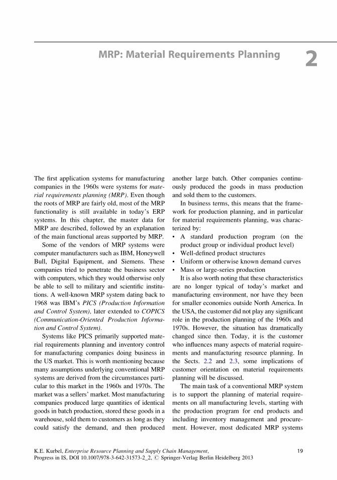
Product Structures Product structures show

what parts make up a product. This composition

is often depicted as a tree. The edges of the tree

represent either “consists of” or “goes into”

relationships, depending on the perspective.

Figure 2.1 shows two simplified product structure

trees for the end products Y and Z. The numbers

on the edges are quantity coefficients. Y consists

of two units of A and one unit of B. Conversely,

A and B go into Y with 2 and 1 units, respectively.

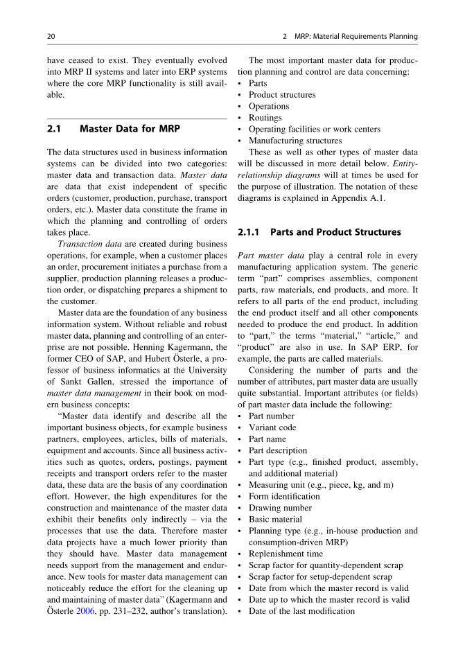
Reversing the perspective, so that the leaves

of one or more product structure trees become

the roots and the end products are the leaves

(“goes into” relationship), creates trees like

those in Fig. 2.2. The figure directly shows

where a given part is needed. For example, part

E goes directly into part A with one unit and into

part C with two units, as well as indirectly into

parts Z, B, and twice (through parts A and B)

into part Y.

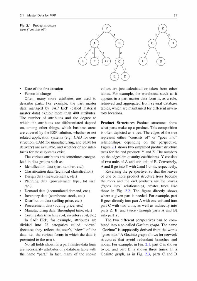
The two different perspectives can be com-

bined into a so-called Gozinto graph. The name

“Gozinto” is supposedly derived from the words

“goes into.” A Gozinto graph allows for network

structures that avoid redundant branches and

nodes. For example, in Fig. 2.1, part C is shown

twice, and part D is shown three times. In a

Gozinto graph, as in Fig. 2.3, parts C and D

Y

A B

E GF C

DE

2 1

1 4 1

2 1

2

Z

C D

E D

2 2

2 1

Fig. 2.1 Product structure

trees (“consists of”)

2.1 Master Data for MRP 21

appear only once. D goes into C and Z, and C

goes into B and Z.

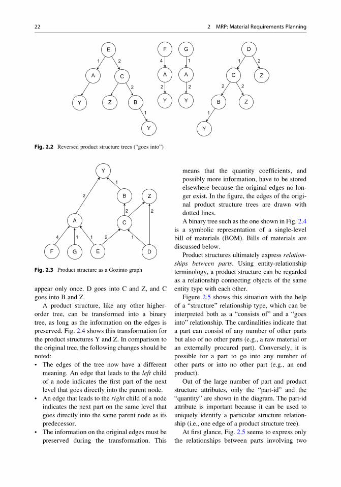
A product structure, like any other higher-

order tree, can be transformed into a binary

tree, as long as the information on the edges is

preserved. Fig. 2.4 shows this transformation for

the product structures Y and Z. In comparison to

the original tree, the following changes should be

noted:

• The edges of the tree now have a different

meaning. An edge that leads to the left childof a node indicates the first part of the next

level that goes directly into the parent node.

• An edge that leads to the right child of a node

indicates the next part on the same level that

goes directly into the same parent node as its

predecessor.

• The information on the original edges must be

preserved during the transformation. This

means that the quantity coefficients, and

possibly more information, have to be stored

elsewhere because the original edges no lon-

ger exist. In the figure, the edges of the origi-

nal product structure trees are drawn with

dotted lines.

A binary tree such as the one shown in Fig. 2.4

is a symbolic representation of a single-level

bill of materials (BOM). Bills of materials are

discussed below.

Product structures ultimately express relation-

ships between parts. Using entity-relationship

terminology, a product structure can be regarded

as a relationship connecting objects of the same

entity type with each other.

Figure 2.5 shows this situation with the help

of a “structure” relationship type, which can be

interpreted both as a “consists of” and a “goes

into” relationship. The cardinalities indicate that

a part can consist of any number of other parts

but also of no other parts (e.g., a raw material or

an externally procured part). Conversely, it is

possible for a part to go into any number of

other parts or into no other part (e.g., an end

product).

Out of the large number of part and product

structure attributes, only the “part-id” and the

“quantity” are shown in the diagram. The part-id

attribute is important because it can be used to

uniquely identify a particular structure relation-

ship (i.e., one edge of a product structure tree).

At first glance, Fig. 2.5 seems to express only

the relationships between parts involving two

E

A C

Y

Y

BZ

1 2

2

1

F

A

Y

G

A

Y

4 1

2 2

D

C

B

Y

Z

Z

1 2

2 2

1

Fig. 2.2 Reversed product structure trees (“goes into”)

Y

A

B

F EG

C

2

4 1 1 2 1

2

1

D

Z

2

Fig. 2.3 Product structure as a Gozinto graph


levels and not the multilevel structures that were

shown in the earlier figures. However, multilevel

structures can be easily generated through appro-

priate database queries. For this purpose, the

part-ids of related subordinate and superordinate

parts are employed to link single-level structures

into a multilevel structure.

The ER model of Fig. 2.5 can be mapped to a

relational database with the help of two tables,

“part” and “structure.” In relational notation (see

Appendix A.2), these two tables are defined as

follows:

Part (part-id, part name, part type, unit of

measurement. . .)Structure (upper-part-id, lower-part-id, quantity,

valid-from. . .)

The “structure” table has a composite key,

indicating the two part entities to be linked.

Graphically speaking, the “upper-part-id” attribute

identifies the parent node in the product structure,

while the “lower-part-id” identifies the child node.

Figure 2.6 exemplifies a product structure tree

of an electric motor with part number “E10.”

Figure 2.7, which is based on this product

structure, exhibits two tables—one with the

parts and the other with the relationships between

parts—according to the E10 product structure.

The part table shows, along with the part

number (“part-id”), three additional attributes.

The “part type” attribute has values that are

abbreviations of in-house production (I), external

procurement (E), end product (P), assembly (A),

raw material (R), consumables (C), etc. For

example, ER stands for external procurement/

raw material.

In the “structure” table, the first line uniquely

identifies the edge between the end product

“electric motor” (upper-part-id “E10”) and the

assembly “complete casing” (lower-part-id

“901”). The most important attribute of the struc-

ture relationship, in addition to the keys, is the

quantity.

A number of other attributes may also appear

in a “structure” table. Just as with the part master

data, the type and number of attributes are depen-

dent upon the level of detail and the application

environment. Typical fields of a structure table

include:

Y

A B

E GF C

DE

2 1

1 4 1

2 1

2

Z

C D

E D

2 2

2 1

Fig. 2.4 Product structure,

transformed into a binary

tree

Part

Structure

Part-id

Quantity

(0, )

"consists of" "goes into"

(0, )

Fig. 2.5 Product structure

as a relationship type in an

ER diagram


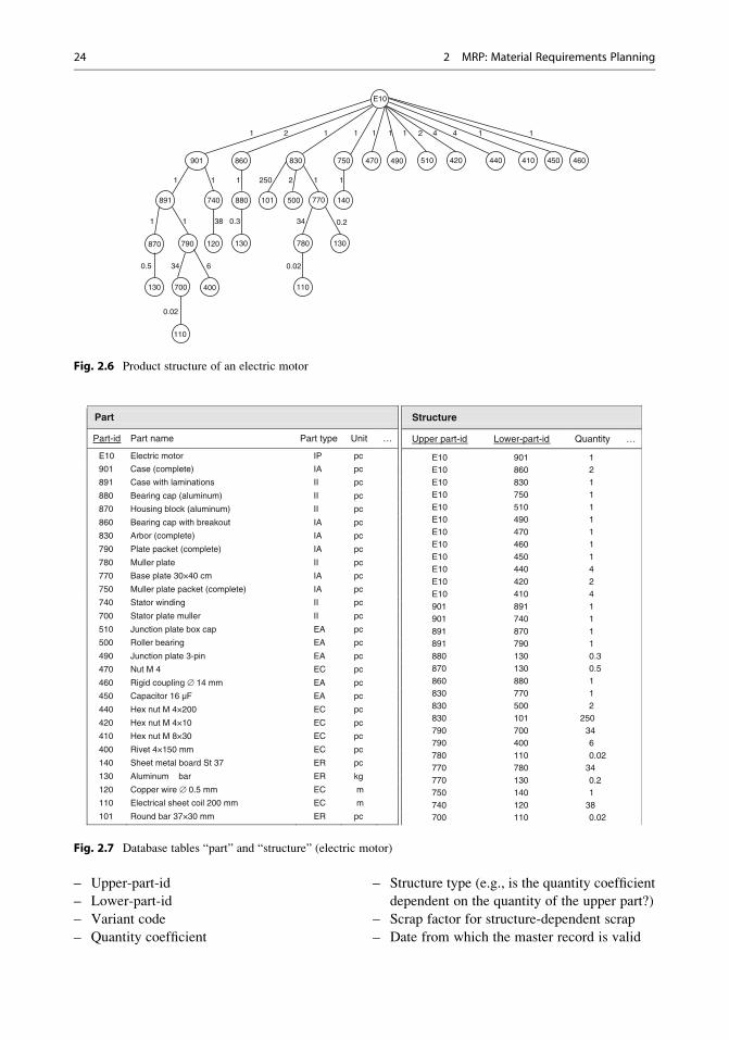
– Upper-part-id

– Lower-part-id

– Variant code

– Quantity coefficient

– Structure type (e.g., is the quantity coefficient

dependent on the quantity of the upper part?)

– Scrap factor for structure-dependent scrap

– Date from which the master record is valid

0.5

870

130

460450410440420510490470750

E10

901 860

140891 740 880 101 500 770

790 120 130 780 130

700 400 110

110

114421111121

112250111

0.2340.33811

0.02634

0.02

830

Fig. 2.6 Product structure of an electric motor

Structure

Upper part-id Lower-part-id Quantity …

E10 901 1E10 860 2E10 830 1E10 750 1E10 510 1E10 490 1E10 470 1E10 460 1E10 450 1E10 440 4E10 420 2E10 410 4901 891 1901 740 1891 870 1891 790 1880 130 0.3870 130 0.5860 880 1830 770 1830 500 2830 101 250790 700 34790 400 6780 110 0.02770 780 34770 130 0.2750 140 1740 120 38700 110 0.02

Part

Part-id Part name Part type Unit …

E10 Electric motor IP pc

901 Case (complete) IA pc

891 Case with laminations II pc

880 Bearing cap (aluminum) II pc

870 Housing block (aluminum) II pc

860 Bearing cap with breakout IA pc

830 Arbor (complete) IA pc

790 Plate packet (complete) IA pc

780 Muller plate II pc

770 Base plate 30×40 cm IA pc

750 Muller plate packet (complete) IA pc

740 Stator winding II pc

700 Stator plate muller II pc

510 Junction plate box cap EA pc

500 Roller bearing EA pc

490 Junction plate 3-pin EA pc

470 Nut M 4 EC pc

460 Rigid coupling ∅ 14 mm EA pc

450 Capacitor 16 µF EA pc

440 Hex nut M 4×200 EC pc



400 Rivet 4×150 mm EC pc

140 Sheet metal board St 37 ER pc

130 Aluminum bar ER kg

120 Copper wire ∅ 0.5 mm EC m

110 Electrical sheet coil 200 mm EC m

101 Round bar 37×30 mm ER pc

Fig. 2.7 Database tables “part” and “structure” (electric motor)


– Date to which the master record is valid

– Date of the last modification

– Date of the first creation

– Person in charge

Important uses of product structures include

(1) compiling bills of materials and where-used

lists and (2) determining dependent requirements

for material planning.

Dependent material requirements, that is, the

quantities of lower-level parts needed to produce

the planned end products (or other higher-level

parts), are calculated with the help of the quantity

coefficients, which are stored in the “quantity”

column of the “structure” table. Sect. 2.3.2 will

discuss the calculation process in more detail.

Bills of Materials A bill of materials (BOM)

represents a product structure together with

essential information about the nodes (i.e., part

master data) in the form of a list. Each row shows

one subordinate part. The parts are described by

part number, part name, quantity needed for the

upper part, etc. In this way, a bill of materials

describes the composition of an end product or an

intermediate product (assembly).

Bills of materials are especially relevant in

discrete manufacturing, that is, in manufacturing

processes in which the quantities are mostly

measured in discrete units (pieces). This is typi-

cally the case when assembly plays a dominant

role, for example, in the production of machines,

bicycles, or furniture.

The opposite of discrete manufacturing is con-

tinuous manufacturing, which occurs particularly

in the chemical and pharmaceutical industry.

There, the equivalent of a bill of materials is a

formulation. The main difference between a bill of

materials and a formulation is that the quantities

are measured in continuous units (kilogram, ton,

liter, etc.) and that the product structure graphs

are not necessarily trees but may contain cycles.

A cycle means that in order to manufacture a

product, the product itself is needed.

In this book, we will focus on discrete

manufacturing using bills of materials, although

a number of similar problems also occur in

continuous manufacturing.

Bills of materials are employed for various

purposes: requirements planning, assembly, com-

puter-aided design, etc. The content, structure,

and format of a bill of materials depend on the

intended use. Hence, a number of labels exist, for

example, planning BOM, assembly BOM, manu-

facturing BOM etc.

Different types of bills of materials exhibit

different structures, depending on how much

structural information is mapped to the bill.

Relating to this, three types can be determined:

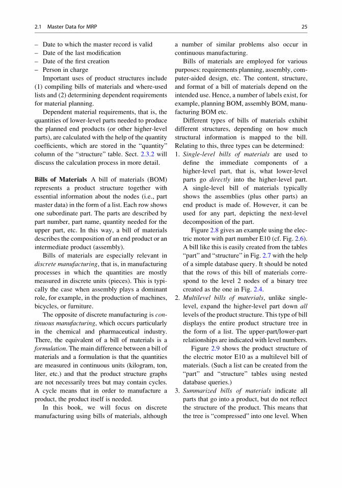
1. Single-level bills of materials are used to

define the immediate components of a

higher-level part, that is, what lower-level

parts go directly into the higher-level part.

A single-level bill of materials typically

shows the assemblies (plus other parts) an

end product is made of. However, it can be

used for any part, depicting the next-level

decomposition of the part.

Figure 2.8 gives an example using the elec-

tric motor with part number E10 (cf. Fig. 2.6).

A bill like this is easily created from the tables

“part” and “structure” in Fig. 2.7 with the help

of a simple database query. It should be noted

that the rows of this bill of materials corre-

spond to the level 2 nodes of a binary tree

created as the one in Fig. 2.4.

2. Multilevel bills of materials, unlike single-

level, expand the higher-level part down all

levels of the product structure. This type of bill

displays the entire product structure tree in

the form of a list. The upper-part/lower-part

relationships are indicated with level numbers.

Figure 2.9 shows the product structure of

the electric motor E10 as a multilevel bill of

materials. (Such a list can be created from the

“part” and “structure” tables using nested

database queries.)

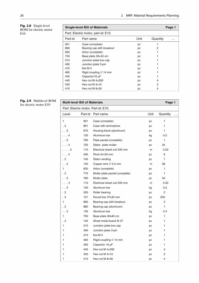
3. Summarized bills of materials indicate all

parts that go into a product, but do not reflect

the structure of the product. This means that

the tree is “compressed” into one level. When


Single-level Bill of Materials Page 1

Part: Electric motor, part-id: E10

Part-id Part name Unit Quantity …

901 Case (complete) pc 1860 Bearing cap with breakout pc 2

830 Arbor (complete) pc 1

750 Base plate 30×40 cm pc 1

510 Junction plate box cap pc 1

490 Junction plate 3-pin pc 1

470 Nut M 4 pc 1

460 Rigid coupling Æ 14 mm pc 1

450 Capacitor16 µF pc 1

440 Hex nut M 4×200 pc 4

420 Hex nut M 4×10 pc 2

410 Hex nut M 8×30 pc 4

Fig. 2.8 Single-level

BOM for electric motor

E10

Multi-level Bill of Materials Page 1

Part: Electric motor, Part-id: E10

Level Part-id Part name Unit Quantity …

1 901 Case (complete) pc 1

. 2 891 Case with laminations pc 1

. . 3 870 Housing block (aluminum) pc 1

. . . 4 130 Aluminum bar kg 0.5

. . 3 790 Plate packet (complete) pc 1

. . . 4 700 Stator plate muller pc 34

. . . . 5 110 Electrical sheet coil 200 mm m 0.02

. . . 4 400 Rivet 4x150 mm pc 6

. 2 740 Stator winding pc 1

. . 3 120 Copper wire Æ 0.5 mm m 38

1 830 Arbor (complete) pc 1

. 2 770 Muller plate packet (complete) pc 1

. . 3 780 Muller plate pc 34

. . . 4 110 Electrical sheet coil 200 mm m 0.02

. . 3 130 Aluminum bar kg 0.2

. 2 500 Roller bearing pc 2

. 2 101 Round bar 37x30 mm pc 250

1 860 Bearing cap with breakout pc 2

. 2 880 Bearing cap (aluminum) pc 1

. . 3 130 Aluminum bar kg 0.3

1 750 Base plate 30x40 cm pc 1

. 2 140 Sheet metal board St 37 pc 1

1 510 Junction plate box cap pc 1

1 490 Junction plate 3-pin pc 1

1 470 Nut M 4 pc 1

1 460 Rigid coupling Æ 14 mm pc 1

1 450 Capacitor 16 µF pc 1

1 440 Hex nut M 4×200 pc 4

1 420 Hex nut M 4×10 pc 2

1 410 Hex nut M 8×30 pc 4

Fig. 2.9 Multilevel BOM

for electric motor E10


a part appears more than once in the product

structure, its quantities are added. Conse-

quently, the bill shows only the total quantity

needed for one unit of the top part (e.g., the

end product). Figure 2.10 illustrates this,

again using the electric motor example.

The part numbers 880, 130, and 110 are exam-

ples showing how several quantities are summar-

ized into one. Because one piece of 880 (bearing

cap) is needed for one 860 (bearing cap with

breakout) and two pieces of 860 are needed for

one E10 (electric motor), the result is that two

pieces of 880 are needed for one E10.

How many units of 130 (aluminum bar) are

needed for one electric motor E10 can be calcu-

lated by multiplying the quantity coefficients on

the edges

870–130 (0.5) and 880–130 (0.3) and 770–130 (0.2)

891–870 (1) 860–880 (1) 830–770 (1)

901–891 (1) E10–860 (2) E10–830 (1)

E10–901 (1)

and adding up the products

0.5 � 1 � 1 � 1 + 0.3 � 1 � 2 + 0.2 � 1 � 1

to 1.3 kg. (This total is shown in the fourth to

the last line in the summarized bill of materials in

Fig. 2.10).

Where-Used Lists While bills of materials

reflect “consists of” relationships between parts,

Summarized Bill of Materials Page 1

Part: Electric motor, Part-id: E10


901 Case (complete) pc 1

891 Case with laminations pc 1

880 Bearing cap (aluminum) pc 2

870 Housing block (aluminum) pc 1

860 Bearing cap with breakout pc 2

830 Arbor (complete) pc 1

790 Plate packet (complete) pc 1

780 Muller plate pc 34

770 Muller plate packet (complete) pc 1

750 Base plate 30×40 cm pc 1

740 Stator winding pc 1

700 Stator plate muller pc 34

510 Junction plate box cap pc 1

500 Roller bearing pc 2

490 Junction plate 3-pin pc 1

470 Nut M 4 pc 1

460 Rigid coupling Æ 14 mm pc 1

450 Capacitor 16 µF pc 1

440 Hex nut M 4×200 pc 4

420 Hex nut M 4×10 pc 2

410 Hex nut M 8×30 pc 4

400 Rivet 4×150 mm pc 6

140 Sheet metal board St 37 pc 1

130 Aluminum bar kg 1.3

120 Copper wire Æ 0.5 mm m 38

110 Electrical sheet coil 200 mm m 1.36

101 Round bar 37×30 mm pc 250

Fig. 2.10 Summarized

BOM for electric motor

E10


where-used lists (part-usage lists) represent

“goes into” relationships. Let us take another

look at Fig. 2.2. This figure shows that reverse

product structure trees can be constructed based

on the “goes into” relationships.

As for bills of materials, different types of

where-used lists can be identified, according to

the degree to which the multilevel structure of

the trees is reflected:

• Single-level where-used lists comprise all

parts into which the given part goes directly.

For example, the list for part 130 (aluminum

bar, cf. Fig. 2.6) would display parts 870 (with

0.5 units), 880 (with 0.3 units), and 770 (with

0.2 units).

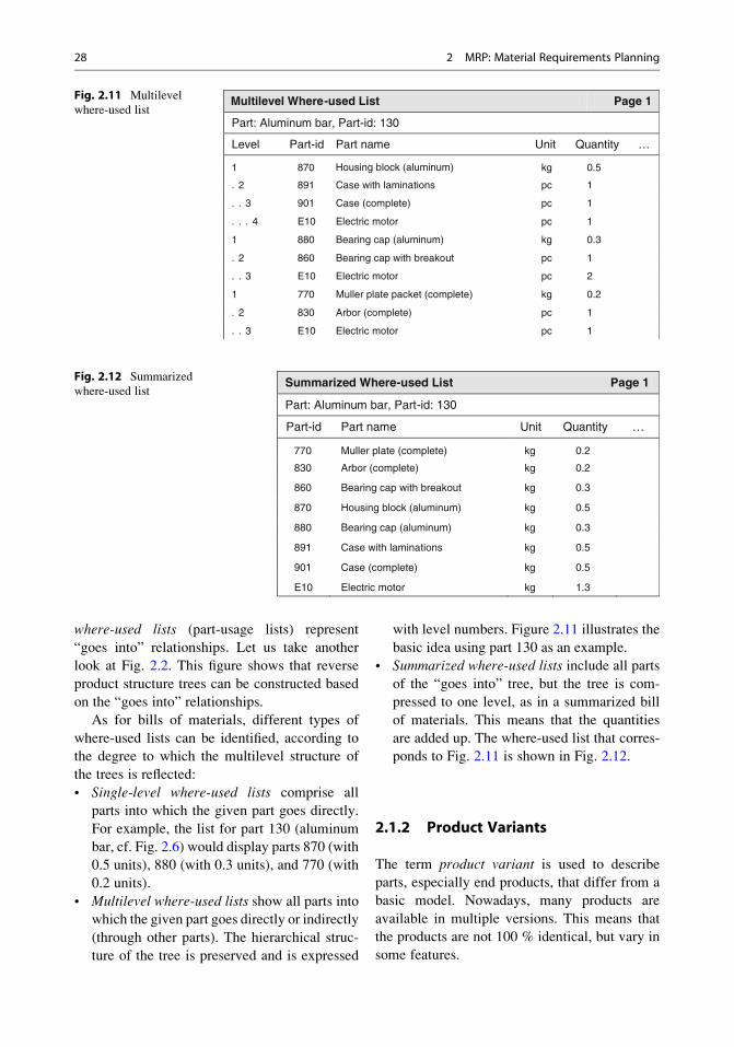
• Multilevel where-used lists show all parts into

which the given part goes directly or indirectly

(through other parts). The hierarchical struc-

ture of the tree is preserved and is expressed

with level numbers. Figure 2.11 illustrates the

basic idea using part 130 as an example.

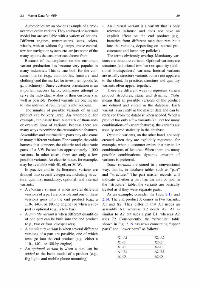
• Summarized where-used lists include all parts

of the “goes into” tree, but the tree is com-

pressed to one level, as in a summarized bill

of materials. This means that the quantities

are added up. The where-used list that corres-

ponds to Fig. 2.11 is shown in Fig. 2.12.

2.1.2 Product Variants

The term product variant is used to describe

parts, especially end products, that differ from a

basic model. Nowadays, many products are

available in multiple versions. This means that

the products are not 100 % identical, but vary in

some features.

Multilevel Where-used List Page 1

Part: Aluminum bar, Part-id: 130

Level Part-id Part name Unit Quantity …

1 870 Housing block (aluminum) kg 0.5

. 2 891 Case with laminations pc 1

. . 3 901 Case (complete) pc 1

. . . 4 E10 Electric motor pc 1

1 880 Bearing cap (aluminum) kg 0.3

. 2 860 Bearing cap with breakout pc 1

. . 3 E10 Electric motor pc 2

1 770 Muller plate packet (complete) kg 0.2

. 2 830 Arbor (complete) pc 1

. . 3 E10 Electric motor pc 1

Fig. 2.11 Multilevel

where-used list

Summarized Where-used List Page 1

Part: Aluminum bar, Part-id: 130


770 Muller plate (complete) kg 0.2

830 Arbor (complete) kg 0.2

860 Bearing cap with breakout kg 0.3

870 Housing block (aluminum) kg 0.5

880 Bearing cap (aluminum) kg 0.3

891 Case with laminations kg 0.5

901 Case (complete) kg 0.5

E10 Electric motor kg 1.3

Fig. 2.12 Summarized

where-used list


Automobiles are an obvious example of a prod-

uct produced in variants. They are based on a certain

model but are available with a variety of options.

Different engines, transmissions, seats, colors,

wheels, with or without fog lamps, cruise control,

tow bar, navigation system, etc. are just some of the

many options the customer can choose from.

Because of the emphasis on the customer,

variant production has become very popular in

many industries. This is true both for the con-

sumer market (e.g., automobiles, furniture, and

clothing) and the market for investment goods (e.

g., machinery). Since customer orientation is an

important success factor, companies attempt to

serve the individual wishes of their customers as

well as possible. Product variants are one means

to take individual requirements into account.

The number of possible variants of an end

product can be very large. An automobile, for

example, can easily have hundreds of thousands

or even millions of variants, because there are

many ways to combine the customizable features.

Assemblies and intermediate parts may also come

in many different variants. For example, the cable

harness that connects the electric and electronic

parts of a VW Passat has approximately 1,000

variants. In other cases, there are only a few

possible variants. An electric motor, for example,

may be available with 40, 60, or 80 W.

In practice and in the literature, variants are

divided into several categories, including struc-

ture, quantity, mandatory, optional, and internal

variants:

• A structure variant is when several different

versions of a part are possible and one of these

versions goes into the end product (e.g., a

110-, 140-, or 180-hp engine) or when a sub-

part is optional (e.g., a tow bar).

• A quantity variant is when different quantitiesof one part can be built into the end product

(e.g., two or four loudspeakers).

• A mandatory variant is when several differentversions of a part are possible, one of which

must go into the end product (e.g., either a

110-, 140-, or 180-hp engine).

• An optional variant is when a part can be

added to the basic model of a product (e.g.,

fog lights and mobile phone mounting).

• An internal variant is a variant that is only

relevant in-house and does not have an

explicit effect on the end product (e.g.,

batteries from different manufacturers built

into the vehicles, depending on internal pro-

curement and inventory policies).

The terms obviously overlap. Mandatory var-

iants are structure variants. Optional variants are

structure (additional tow bar) or quantity (addi-

tional loudspeakers) variants. Internal variants

are usually structure variants but are not apparent

to the client. In practice, structure and quantity

variants often appear together.

There are different ways to represent variant

product structures: static and dynamic. Static

means that all possible versions of the product

are defined and stored in the database. Each

variant is an entity in the master data and can be

retrieved from the database when needed.When a

product has only a few variants (i.e., not too many

combinations of variant features), the variants are

usually stored statically in the database.

Dynamic variants, on the other hand, are only

created when they are explicitly requested, for

example, when a customer orders that particular

combinations of features. When there are many

possible combinations, dynamic creation of

variants is preferred.

Static variants are stored in a conventional

way, that is, in database tables such as “part”

and “structure.” The part master records will

indicate whether a part has variants or not. In

the “structure” table, the variants are basically

treated as if they were separate parts.

As an example, consider the Figs. 2.13 and

2.14. The end product X comes in two variants,

X1 and X2. They differ in that X1 needs an

assembly A1, whereas X2 needs A2. A1 is

similar to A2 but uses a part E1, whereas A2

uses E2. Consequently, the “structure” table

shown in Fig. 2.15 has rows connecting “upper

parts” and “lower parts” as follows:

X1–A1 X2–A2

X1–B X2–B

X1–C X2–C

A1–E1 A2–E2

A1–D A2–D


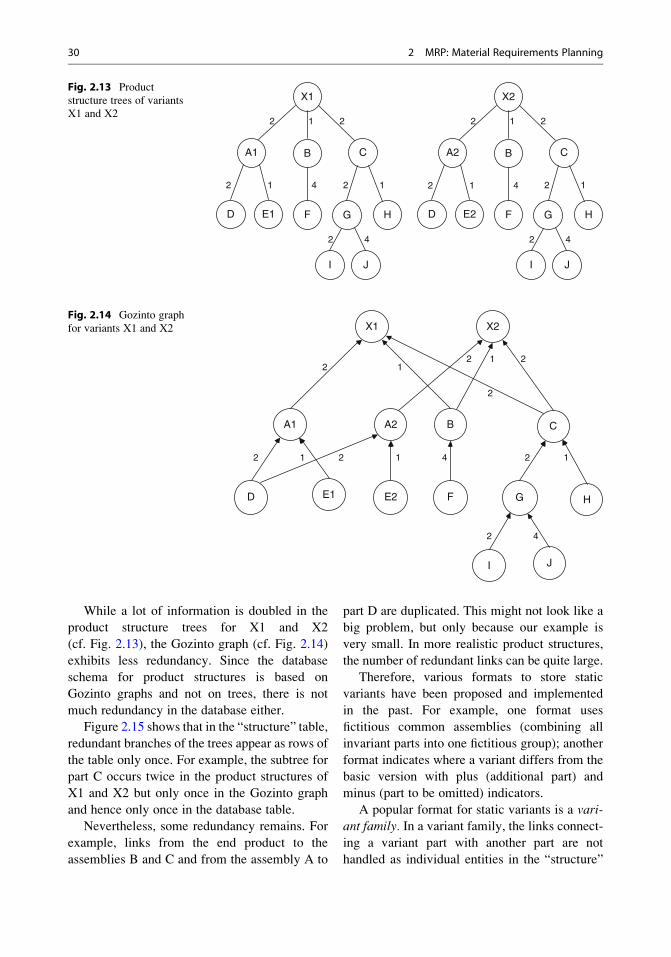
While a lot of information is doubled in the

product structure trees for X1 and X2

(cf. Fig. 2.13), the Gozinto graph (cf. Fig. 2.14)

exhibits less redundancy. Since the database

schema for product structures is based on

Gozinto graphs and not on trees, there is not

much redundancy in the database either.

Figure 2.15 shows that in the “structure” table,

redundant branches of the trees appear as rows of

the table only once. For example, the subtree for

part C occurs twice in the product structures of

X1 and X2 but only once in the Gozinto graph

and hence only once in the database table.

Nevertheless, some redundancy remains. For

example, links from the end product to the

assemblies B and C and from the assembly A to

part D are duplicated. This might not look like a

big problem, but only because our example is

very small. In more realistic product structures,

the number of redundant links can be quite large.

Therefore, various formats to store static

variants have been proposed and implemented

in the past. For example, one format uses

fictitious common assemblies (combining all

invariant parts into one fictitious group); another

format indicates where a variant differs from the

basic version with plus (additional part) and

minus (part to be omitted) indicators.

A popular format for static variants is a vari-ant family. In a variant family, the links connect-

ing a variant part with another part are not

handled as individual entities in the “structure”

2 1 4

X2

A2 C

D E2 G

JI

2 1 2

2 4

2 1

B

F H

X1

A1 C

D E1 G

JI

2 1 2

2 1 4

2 4

2 1

B

F H

Fig. 2.13 Product

structure trees of variants

X1 and X2

D HGE2E1 F

A1 A2 B C

I J

X1 X2

2 1 2 1 4 2 1

2 4

2 12 1 2

2

Fig. 2.14 Gozinto graph

for variants X1 and X2


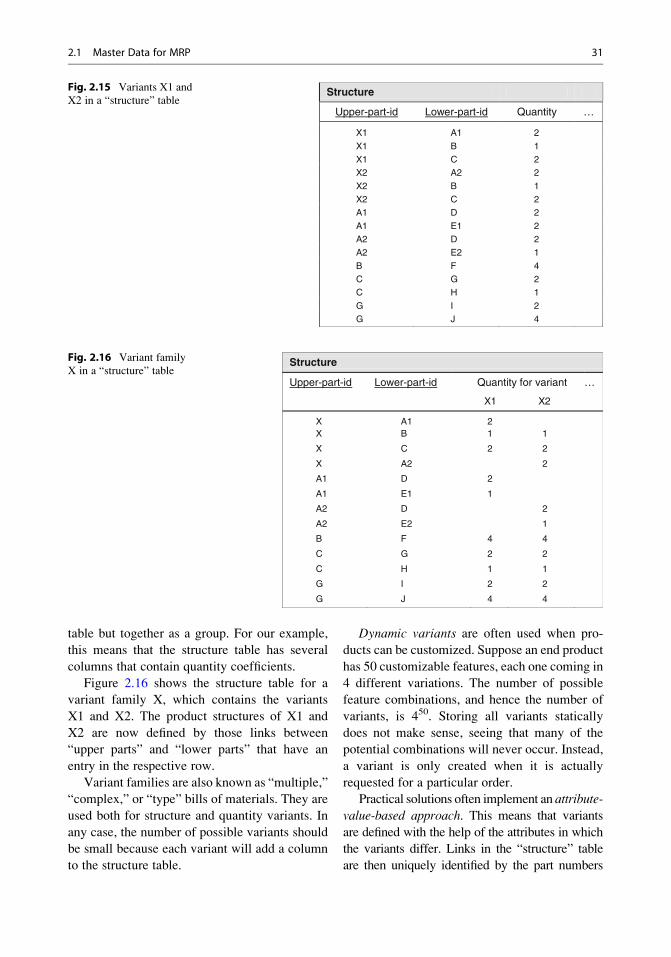
table but together as a group. For our example,

this means that the structure table has several

columns that contain quantity coefficients.

Figure 2.16 shows the structure table for a

variant family X, which contains the variants

X1 and X2. The product structures of X1 and

X2 are now defined by those links between

“upper parts” and “lower parts” that have an

entry in the respective row.

Variant families are also known as “multiple,”

“complex,” or “type” bills of materials. They are

used both for structure and quantity variants. In

any case, the number of possible variants should

be small because each variant will add a column

to the structure table.

Dynamic variants are often used when pro-

ducts can be customized. Suppose an end product

has 50 customizable features, each one coming in

4 different variations. The number of possible

feature combinations, and hence the number of

variants, is 450. Storing all variants statically

does not make sense, seeing that many of the

potential combinations will never occur. Instead,

a variant is only created when it is actually

requested for a particular order.

Practical solutions often implement an attribute-

value-based approach. This means that variants

are defined with the help of the attributes in which

the variants differ. Links in the “structure” table

are then uniquely identified by the part numbers

Structure

Upper-part-id Lower-part-id Quantity …

X1 A1 2

X1 B 1X1 C 2X2 A2 2

X2 B 1X2 C 2A1 D 2

A1 E1 2A2 D 2A2 E2 1

B F 4C G 2C H 1

G I 2G J 4

Fig. 2.15 Variants X1 and

X2 in a “structure” table

Structure

Upper-part-id Lower-part-id Quantity for variant …

X1 X2

X A1 2X B 1 1

X C 2 2

X A2 2

A1 D 2

A1 E1 1

A2 D 2

A2 E2 1

B F 4 4

C G 2 2

C H 1 1

G I 2 2

G J 4 4

Fig. 2.16 Variant family

X in a “structure” table


of the upper and the lower parts, plus a variant code

that defines the attributes of the specific variant

under consideration. (In relational terminology,

this means that the variant code is also a key attri-

bute.) In this way, variant-specific parts can be

marked and tracked down the product structure

any number of manufacturing levels.

As an example, let us assume that variant X2

differs from X1 in that the color of assembly

group A2 is green (instead of red in A1 or white

in another variant) and the power of E2 is 80 kW

(instead of 40 kW in E1 or 60 in another variant):

Attribute Value

Color Green

Red

White

Power 40

60

80

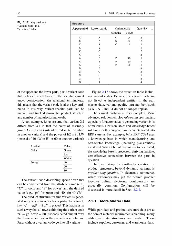
The variant code describing specific variants

can be constructed from the attribute name (e.g.,

“C” for color and “P” for power) and the desired

value (e.g., “gr” for green and “40” for 40 kW).

The product structure for this variant is gener-

ated only when an order for a particular variant,

say “C ¼ gr/P ¼ 80,” is placed. This happens in

such away that all rows exhibiting the variant code

“C ¼ gr” or “P ¼ 80” are considered plus all rows

that have no entries in the variant-code columns.

Parts without a variant code go into all variants.

Figure 2.17 shows the structure table includ-

ing variant codes. Because the variant parts are

not listed as independent entities in the part

master data, variant-specific part numbers such

as X1, A1, and E1 do not no longer appear.

The variant problem is very complex. More

advanced solutions employ rule-based approaches,especially for automatically generating variant bills

of materials. Decision tables and knowledge-based

solutions for this purpose have been integrated into

ERP systems. For example, Infor ERP COM uses

a knowledge base in which manufacturing and

cost-related knowledge (including plausibilities)

are stored. When a bill of materials is to be created,

the knowledge base is processed, deriving feasible,

cost-effective connections between the parts in

question.

The next stage in on-the-fly creation of

product structures, beyond dynamic variants, is

product configuration. In electronic commerce,

where customers may put the desired product

together online, electronic configurators are

especially common. Configuration will be

discussed in more detail in Sect. 2.2.2.

2.1.3 More Master Data

While part data and product structure data are at

the core of material requirements planning, many

additional data structures are needed. These

include supplier, customer, and warehouse data.

Structure

Upper-part-id Lower-part-id Variant code Quantity …

Attribute Value

X A C gr 2

X A C re 2

X A C bl 2

X B 1

X C 2

A D 2

A E P 40 1

A E P 60 1

A E P 80 1

B F 4

C G 2

C H 1

G I 2

G J 4

Fig. 2.17 Key attribute

“variant code” in a

“structure” table


Suppliers Supplier data are used in material

requirements planning for procurement and

purchase orders. Typical attributes of a supplier

include:

• Supplier number

• Supplier name

• Address

• Contact person

• Payment data

• Supplier rating (e.g., percent of deliveries

being disputed, quality, and average delay

time)

• Liability limit

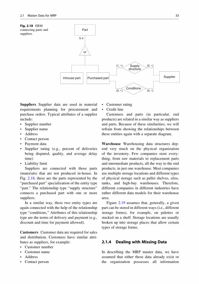
Suppliers are connected with those parts

(materials) that are not produced in-house. In

Fig. 2.18, these are the parts represented by the

“purchased part” specialization of the entity type

“part.” The relationship type “supply structure”

connects a purchased part with one or more

suppliers.

In a similar way, these two entity types are

again connected with the help of the relationship

type “conditions.” Attributes of this relationship

type are the terms of delivery and payment (e.g.,

discount and time for payment allowed).

Customers Customer data are required for sales

and distribution. Customers have similar attri-

butes as suppliers, for example:

• Customer number

• Customer name

• Address

• Contact person

• Customer rating

• Credit line

Customers and parts (in particular, end

products) are related in a similar way as suppliers

and parts. Because of these similarities, we will

refrain from showing the relationships between

these entities again with a separate diagram.

Warehouse Warehousing data structures dep-

end very much on the physical organization

of the inventory. Few companies store every-

thing, from raw materials to replacement parts

and intermediate products, all the way to the end

products, in just one warehouse. Most companies

use multiple storage locations and different types

of physical storage such as pallet shelves, silos,

tanks, and high-bay warehouses. Therefore,

different companies in different industries have

rather different data models for their warehouse

area.

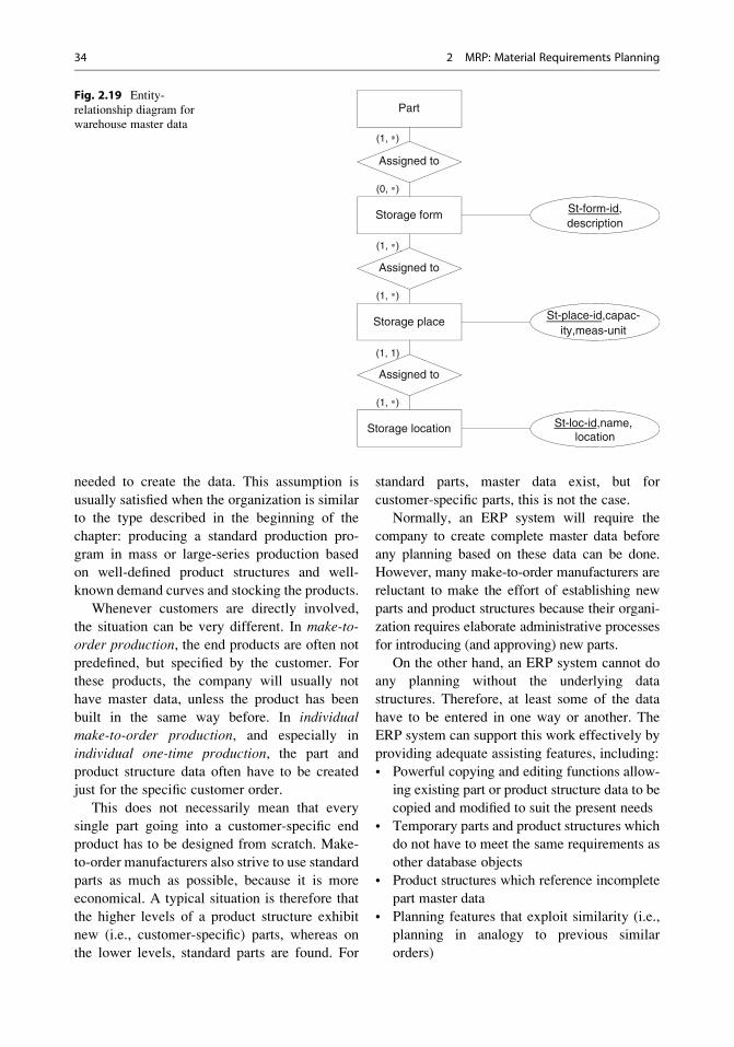
Figure 2.19 assumes that, generally, a given

part can be stored in different ways (i.e., different

storage forms), for example, on palettes or

stacked on a shelf. Storage locations are usually

broken up into storage places that allow certain

types of storage forms.

2.1.4 Dealing with Missing Data

In describing the MRP master data, we have

assumed that either these data already exist or

the organization possesses all information

Part

(1, ) (0, )

is a

or

Inhouse part Purchased part

Supplystructure

Conditions

Supplier

(0, )(0, )

Fig. 2.18 ERM

connecting parts and

suppliers


needed to create the data. This assumption is

usually satisfied when the organization is similar

to the type described in the beginning of the

chapter: producing a standard production pro-

gram in mass or large-series production based

on well-defined product structures and well-

known demand curves and stocking the products.

Whenever customers are directly involved,

the situation can be very different. In make-to-

order production, the end products are often not

predefined, but specified by the customer. For

these products, the company will usually not

have master data, unless the product has been

built in the same way before. In individualmake-to-order production, and especially in

individual one-time production, the part and

product structure data often have to be created

just for the specific customer order.

This does not necessarily mean that every

single part going into a customer-specific end

product has to be designed from scratch. Make-

to-order manufacturers also strive to use standard

parts as much as possible, because it is more

economical. A typical situation is therefore that

the higher levels of a product structure exhibit

new (i.e., customer-specific) parts, whereas on

the lower levels, standard parts are found. For

standard parts, master data exist, but for

customer-specific parts, this is not the case.

Normally, an ERP system will require the

company to create complete master data before

any planning based on these data can be done.

However, many make-to-order manufacturers are

reluctant to make the effort of establishing new

parts and product structures because their organi-

zation requires elaborate administrative processes

for introducing (and approving) new parts.

On the other hand, an ERP system cannot do

any planning without the underlying data

structures. Therefore, at least some of the data

have to be entered in one way or another. The

ERP system can support this work effectively by

providing adequate assisting features, including:

• Powerful copying and editing functions allow-

ing existing part or product structure data to be

copied and modified to suit the present needs

• Temporary parts and product structures which

do not have to meet the same requirements as

other database objects

• Product structures which reference incomplete

part master data

• Planning features that exploit similarity (i.e.,

planning in analogy to previous similar

orders)

Part

Assigned to

(1, )

Storage form

Storage place

Storage location

(0, )

Assigned to

(1, )

(1, )

Assigned to

(1, 1)

(1, )

St-form-id,description

St-place-id,capac-ity,meas-unit

St-loc-id,name,location

Fig. 2.19 Entity-

relationship diagram for

warehouse master data


2.1.5 A Note on “Numbers”

In the previous sections, so-called numbers were

employed to identify the parts (materials) in

material requirements planning. These numbers

are present in the master data, product structures,

bills of materials, where-used lists, and in many

more places. Likewise, all other objects of enter-

prise resource planning, such as machines, rout-

ings, tools, orders, invoices, and customers, are

identified by numbers.

Althoughwe usually speak of “numbers,” these

numbers are not meant to be used as numerical

values in computations nor are they exclusively

composed of numerical digits. In the electricmotor

example above, the part number was “E10.” The

reader will find more examples of numbers (i.e.,

article numbers) by looking at any sales slip

printed by a supermarket’s cash register.

Many numbers contain long sequences of

digits, and also letters, dashes, and other nonnu-

meric characters. The reason for these long

strings is that the numbers serve more purposes

than just identifying an object. In general, the

purpose of a number can be:

• Identification—the number only identifies an

object

• Classification—the number shows which cat-

egory of objects the object belongs to

• Information—the number tells what the

object is (so-called mnemonic number)

According to this distinction, different types

of numbering systems have been developed and

put into practice:

1. Identification numbers serve the sole purpose of

uniquely identifying an object. The simplest

numbering scheme for this is to use serial

integer numbers starting with 1. Although text-

book examples sometimes use this scheme, it is

not typical for real-world applications.

2. Classification numbers categorize objects, that

is, they are structured in a way that some places

of the number are reserved for the category the

object belongs to, other places for the subcate-

gory, etc. For example, a numbering scheme

may prescribe that the first two places are for

the overall category of the part, the next three

places for a form identifier, and the next three

places for the basic material the part is made of.

A part number would then be composed of

three components: xx-xxx-xxx (e.g., 10-C12-

133). Obviously such a number is generally not

unique because there may be more than one

part in the same subgroup.

3. Compound numbers extend classification

numbers by an identifying number within the

subgroup in order to make the number unique.

Figure 2.20 shows an example. In addition to

the classifying components, a serial number is

used to uniquely identify the parts within sub-

group 03 (rotary drive) of crane 17’s carriage.

It should be noted that the identifying part of

the number is only unique within the subgroup

03, not within the entire part spectrum.

4. Parallel numbers do two things parallel and

independently from each other: They classify

a part and identify it at the same time. This

means that the identifying number is unique

M 1 2 0 1 72 4 0 3

Classification

Identification

Part: bolt (serial number)

Assembly: rotary drive

Master: carriage

Product: crane 17

Fig. 2.20 Compound

number (example)


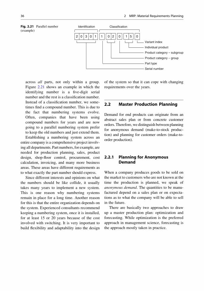
across all parts, not only within a group.

Figure 2.21 shows an example in which the

identifying number is a five-digit serial

number and the rest is a classification number.

Instead of a classification number, we some-

times find a compound number. This is due to

the fact that numbering systems evolve.

Often, companies that have been using

compound numbers for years and are now

going to a parallel numbering system prefer

to keep the old numbers and just extend them.

Establishing a numbering system across an

entire company is a comprehensive project involv-

ing all departments. Part numbers, for example, are

needed for production planning, sales, product

design, shop-floor control, procurement, cost

calculation, invoicing, and many more business

areas. These areas have different requirements as

to what exactly the part number should express.

Since different interests and opinions on what

the numbers should be like collide, it usually

takes many years to implement a new system.

This is one reason why numbering systems

remain in place for a long time. Another reason

for this is that the entire organization depends on

the system. Experienced consultants recommend

keeping a numbering system, once it is installed,

for at least 15 or 20 years because of the cost

involved with switching. It is very important to

build flexibility and adaptability into the design

of the system so that it can cope with changing

requirements over the years.

2.2 Master Production Planning

Demand for end products can originate from an

abstract sales plan or from concrete customer

orders. Therefore, we distinguish between planning

for anonymous demand (make-to-stock produc-

tion) and planning for customer orders (make-to-

order production).

2.2.1 Planning for AnonymousDemand

When a company produces goods to be sold on

the market to customers who are not known at the

time the production is planned, we speak of

anonymous demand. The quantities to be manu-

factured depend on a sales plan or on expecta-

tions as to what the company will be able to sell

in the future.

There are basically two approaches to draw

up a master production plan: optimization and

forecasting. While optimization is the preferred

approach in management science, forecasting is

the approach mostly taken in practice.

1 0 2

ClassificationIdentification

0302 1 0 1 5 0

Variant index

Individual product

Product category – subgroup

Product category – group

Part type

Serial number

Fig. 2.21 Parallel number

(example)


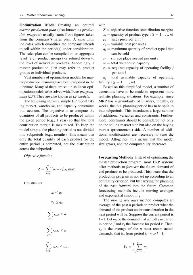
Optimization Model Creating an optimal

master production plan (also known as produc-tion program) usually starts from figures taken

from the company’s sales plan. A sales plan

indicates which quantities the company intends

to sell within the period(s) under consideration.

The sales plan can be compiled on an aggregate

level (e.g., product groups) or refined down to

the level of individual products. Accordingly, a

master production plan may refer to product

groups or individual products.

Vast numbers of optimization models for mas-

ter production planning have been proposed in the

literature. Many of them are set up as linear opti-

mizationmodels to be solvedwith linear program-

ming (LP). They are also known as LP models.The following shows a simple LP model tak-

ing market, warehouse, and capacity constraints

into account. The objective is to compute the

quantities of all products to be produced within

the given period (e.g., 1 year) so that the total

contribution margin is maximized. To keep the

model simple, the planning period is not divided

into subperiods (e.g., months). This means that

only the total quantity of each product for the

entire period is computed, not the distribution

across the subperiods.

Objective function

Z ¼Xni¼1

ðpi � ciÞxi max:

Constraints

xi � q1

xn � qn

Xni¼1

sixi � w

Xni¼1

ri1xi � a1

Xni¼1

rimxi � am;

with

Z ¼ objective function (contribution margin)

xi ¼ quantity of product type i (i ¼ 1, . . ., n)pi ¼ sales price per unit i

ci ¼ variable cost per unit i

qi ¼ maximum quantity of product type i that

can be sold

si ¼ storage place needed per unit i

w ¼ total warehouse capacity

rij ¼ required capacity of operating facility j

per unit i

aj ¼ total available capacity of operating

facility j (j ¼ 1, . . ., m)

Based on this simplified model, a number of

extensions have to be made to represent more

realistic planning situations. For example, since

MRP has a granularity of quarters, months, or

weeks, the total planning period has to be split up

into subperiods. This introduces a large number

of additional variables and constraints. Further-

more, constraints should be considered not only

on the selling market side but also on the buying

market (procurement) side. A number of addi-

tional modifications are necessary to tune the

model. Altogether, this means that the model

size grows, and the computability decreases.

Forecasting Methods Instead of optimizing the

master production program, most ERP systems

offer methods to forecast the future demand of

end products to be produced. This means that the

production program is not set up according to an

optimality criterion, but by carrying the planning

of the past forward into the future. Common

forecasting methods include moving averages

and exponential smoothing.

The moving averages method computes an

average of the past n periods to predict what the

demand of the product under consideration in the

next period will be. Suppose the current period is

k�1. Let mj be the demand that actually occurred

in period j and vk the forecast for period k. Then,

vk is the average of the n most recent actual

demands, that is, from period k�n to k�1:

Vk ¼ 1

n

Xk�1

j¼k�n

mj:

2.2 Master Production Planning 37

This method is called “moving” because one

period later, the average of actual demands now

includes period k, but not k�n, that is, it goes

from k�n+1 to k. Two periods later, the average

refers to periods k�n+2 to k+1, etc.Even though the moving averages method is

extremely simple, it allows for slower or faster

adaption to changing demand. If the parameter n

is stipulated with a small value, then demand

variations are quickly reflected in the forecast.

If n is large, fluctuations are leveled, and outliers

do not much affect the forecast.

In the following example, actual demand values

from 6 past periods are given. Suppose n is 5 and

we want to predict the demand for period 10.

Computing the forecast for this period yields

v10 ¼ 104. If one period later we know that the

actual demand in period 10 was 100, we can

compute the forecast for the next period,

resulting in v11 ¼ 106.

Exponential smoothing is a method that can

be configured to give recent demand fluctuations

more weight than earlier ones. The forecast value

vk is easily calculated: It is equal to the previous

forecast vk�1 plus the weighted deviation of the

actual demand mk�1 from this forecast:

vk ¼ vk�1 þ a mk�1 � vk�1ð Þ:

The weighting factor a is the parameter to

influence the method’s behavior. a can be stipu-

lated with a value between 0 and 1. If a is close to1, the forecast will be close to the actual demand

in period k�1. This means that the forecasting

immediately follows demand fluctuations. The

opposite is true for a small a. This can be seen

by setting a to 0. In this case, demand changes

have no effect at all. The next forecast is the

same as the previous one.

Between the two extremes, there is a range

of possibilities to take recent demand values

into account with great or with little weight

(0 < a < 1). In this way, the demand curve is

smoothed to reflect demand variations either

more or less quickly.

The table below illustrates the effect of different

a values. Starting with period 6 (v5 ¼ 100), v6 is98 if a ¼ 0.2 but only 92 if a ¼ 0.8. Obviously,

the drop in actual demand—forecast v5 is 100 but

actual demand m5 is only 90—is reflected more

immediately when a is larger.

Exponential smoothing as described above

causes the forecasts to follow demand variations,

but not all extreme movements (except if a ¼ 1),

with a time lag. This is acceptable if there are ups

and downs in the actual demand, but if all

demand changes go in one direction, it may be

preferable to catch up with the trend faster.

This can be achieved by smoothing not

only the demand variations but also the forecast

variations. Let

2vk ¼ second-order forecast

1vk ¼ first-order forecast:

The forecast from second-order exponential

smoothing is obtained by first computing the

first-order forecast 1vk as before, then computing

the weighted deviation of the previous period’s

second-order forecast 2vk�1 from1vk and adding

this deviation to 2vk�1:

2vk ¼ 2vk�1 þ a 1vk � 2vk�1

� �:

Period j . . . 4 5 6 7 8 9 10

Demand

mj

. . . 100 90 118 110 105 97 –

Period j . . . 4 5 6 7 8 9 10

Actual demand mj . . . 100 90 118 110 105 97 –

Forecast vkFor a ¼ 0.2 – 100 98 102.0 103.6 103.9 102.5

For a ¼ 0.8 – 100 92 112.8 110.6 106.1 98.8


In this way, the demand variations are

smoothed twice. As a consequence, the forecasts

are adapting faster to the actual demand curve,

provided that the trend goes in one direction (i.e.,

continuously increasing or decreasing).

2.2.2 Planning for Customer Orders

Many companies today produce goods according

to specific customer orders instead of according

to an abstract production program. The previous

section showed how a master production plan

based on anonymous demand can be created.

Now we will discuss what a customer-oriented

manufacturing company has to do to determine

their primary requirements.

Companies relying in their planning on cus-

tomer orders are said to pursue make-to-orderproduction. The majority of small and medium-

sized manufacturing companies work in a

make-to-order style. These companies, unlike

make-to-stock manufacturers who produce stan-

dard goods to be stocked and sold from the ware-

house, produce their goods when customers order

them. This often implies that the customer

specifies what the goods should be like (i.e., the

product specification is provided by the customer).

Make-to-order production is common in the

investment goods sector (e.g., machine tools,

production facilities, cranes, and elevators).

Typical make-to-stock manufacturers are found

in the consumer goods sector (e.g., television

sets, washing machines, and lamps). However,

many consumer goods nowadays are made to

order as well (e.g., cars and personal computers).

Primary requirements planning in make-to-

order production is quite different from make-

to-stock production. Instead of optimizing or

forecasting a standard production program, all

activities are related to specific customer orders.

Typical tasks include scheduling the customer

order to obtain a delivery date, designing the

product the customer wants, calculating the cost

of the product, making a quotation, etc.

Make-to-order production is not a uniform

approach but includes a wide range of options.

These options differ in the degree to which the

planning, execution, and controlling actually

depend on the customer order or are independent

of the order.

For example, a customer may request an end

product that needs to be designed in a specific

way. This does not necessarily mean, however,

that all parts going into that end product must be

designed from scratch. Instead, the company will

try to use as many standard parts as possible to

cut costs. In another company, the situation may

be different, requiring the company to manufac-

ture not only the end product but also assemblies

and individual parts specifically for the customer.

Thus, the spectrum of make-to-order produc-

tion ranges from production types close to make-

to-stock to one-time individual production,

including the following levels:

• Variant production—customers can order

variants of a basic product as discussed in

Sect. 2.1.2.

• Assemble-to-order—customer-specific products

are assembled from standard parts and subas-

semblies.

• Subassemble-to-order—customer-specific

end products as well as customer-specific

assemblies are made from standard subassem-

blies and parts.

• Individual make-to-order—in principle, all

in-house-production parts of a customer-

specific product are manufactured to the cus-

tomer order.

• Individual-purchase-and-make-to-order—all

parts needed for a customer-specific product

(both in-house production and procured parts)

are manufactured and purchased to the

customer order.

• Individual one-time production—this is a

special case of the two previous variants,

meaning that the product is only produced

once in this form as now specified by the

customer (e.g., a ship).

Requirements for Make-to-Order Produc-

tion Make-to-order production gives the customer

a prominent role, in contrast to make-to-stock pro-

duction where customers are not directly involved.


An important objective for the company is to satisfy

the customer. Happy customers will return in the

future and place more orders, which pays more for

the company in the long term than minimizing

production cost or maximizing capacity utilization.

Consequently, the goals of make-to-order pro-

duction focus on customer satisfaction. Essentialsubgoals for production planning are short lead

times, strict adherence to deadlines and delivery

dates, high product quality, and flexibility regard-

ing customer wishes. Pursuing these subgoals

often increases the cost (e.g., overtime work,

machine idle times, and air freight). A make-to-

order manufacturer will normally accept this

increase because the consequences of losing or

disappointing the customer are considered to be

more severe.

Another requirement in make-to-order pro-

duction is that the status of all manufacturing

orders connected with the customer order is

available at all times. When the customer

inquires about their orders, the sales employee

must be able to find out on click what the current

status is. Whenever problems in the plant occur

that affect the customer order (e.g., a bottleneck

machine breaks down), the sales employee must

be immediately informed.

A precondition for employees to be well

informed at any time is transparency of the

manufacturing processes. This requires, for exam-

ple, that all connections between manufacturing

and purchase orders related to a customer order

are explicitly stored. Likewise, all operating facil-

ities involved must be identified. When all con-

nections are available, it is possible to track the

consequences of a problem occurring anywhere in

the order network and to find out whether the

problem will have an impact on the customer

order. In other words, an ERP system suitable

for make-to-order manufacturers has to create

and maintain all connections between the relevant

manufacturing entities.

The ERP system should also be able to work

with incomplete master data. This problem has

already been addressed in Sect. 2.1.4 above.

Working with incomplete master data means

that the ERP system can still perform material

requirements planning, lead-time scheduling,

and capacity planning, even though some of the

underlying data structures (e.g., bills of materials

and routings) are not complete or even missing.

Obviously, the planning results will not be of the

same quality and certainty as if they were based

on complete data, which is the case in make-to-

stock production.

Nevertheless, a make-to-order manufacturer

also needs to plan the production, but the condi-

tions under which the planning takes place are

different from those a make-to-stock manufac-

turer is exposed to. Three crucial planning steps

are:

• Order calculation

• Order scheduling

• Rough-cut planning

In contrast to make-to-stock production, most

make-to-order manufacturers do not have a reli-

able, cost or profit-based production program

from which they can derive the primary require-

ments. Therefore, they have to go other ways to

determine favorable primary requirements that are

in line with the company’s cost or profit goals.

Two important decisions to make in this

process are whether a customer order should be

accepted and for what price. In order to be able to

negotiate a reasonable selling price, the company

needs to know the cost of the order.

Accordingly, order calculation (precalcula-

tion of a customer order) is of utmost importance.

Cost calculation is normally based on master data

such as parts, bills of materials, routings, and

operating facilities (cf. Sect. 3.7.1). If these data

are not available, it is difficult or impossible to

reliably calculate the cost of a prospective order.

Nonconventional approaches have to be applied

to obtain even rough cost data (cf. Sect. 3.7.2).

A problem similar to order calculation is

order scheduling. Scheduling is necessary to

be able to agree on a delivery date with the

customer. Normally, orders are scheduled using

bills of materials and routings, with feasibility of

the schedule being established based on capacity

data (cf. Sects. 3.3 and 3.4). When these data are

not available, other procedures to arrive at a

plausible delivery date must be in place.


http://dx.doi.org/10.1007/978-3-642-31573-2_3#Sec000323




An important prerequisite for smooth manu-

facturing conditions in make-to-order production

is a good rough-cut planning. Since many factors

are still unknown, it is not possible to plan the

customer orders in detail. Therefore, it is impor-

tant to at least balance the overall material and

capacity situation. If this balance can be estab-

lished, it is possible later to schedule customer

orders without (or with fewer) problems. This is,

by the way, one of the fundamental ideas of

manufacturing resource planning (MRP II, cf.

Sect. 3.2), even though MRP II is targeted more

toward make-to-stock than make-to-order pro-

duction.

Product Specification End products in make-

to-order production are typically not standard

products but new or at least different products.

Because the decisions mentioned above con-

cerning price and time can only be made once

the product is “known,” one of the initial steps in

the order fulfillment process (cf. Sect. 4.3.2) is

to create a specification of the product in the

ERP system. This may be done by adopting

the customer’s product specification (if they

already have one), by creating a specification

from scratch and/or by interacting with the cus-

tomer, in order to derive the specification to-

gether.

A product specification is necessary to check

the feasibility of the customer’s product idea

against the company’s technological capabilities

before the customer order is accepted. It is also

needed to create order-specific master data such

as bills of materials and routings, based on which

material and capacity planning can be performed.

One relatively easy way to specify a customer-

dependent product is to employ product variants

as discussed in Sect. 2.1.2. This method, how-

ever, is only applicable when the product ordered

by the customer is within the given spectrum of

variants.

Product configuration goes one step farther

than variant management. A product configura-

tor is a program that allows a knowledgeable user

to put together a product interactively from a set

of given components. The program checks which

combinations of assemblies, individual parts, and

possibly raw materials are permitted and may

recommend especially beneficial combinations.

When complex products are involved, there

may be many rules and regulations that have to

be considered. Human experts configuring these

products are aware of the rules and regulations

that may apply. A good product configurator

produces results that come close to those of the

human experts or in some cases even exceed

them.

Product configuration was one of the first

domains in which knowledge-based systems,especially expert systems, were successfully

applied. The first configuration systems were

developed in the 1980s for putting together

computer systems, such as Digital Equipment’s

XCON [also known as R1 (McDermott 1981)].

These were followed by a large number of

configurators for a variety of products (turbines,

elevators, roller blinds, etc.).

Today, configuration systems are very com-

mon in electronic commerce, allowing customers

to select which features of the product they prefer.

The configuration program in the background

checks whether the selected combination of

features is feasible or allows the customer to select

only those features that may be combined.

Product configurators can appear as separate

systems or be integrated in an ERP system.

Typical functionality of an interactive configura-

tion module includes (Hullenkremer 2003):

• Configuration on the basis of rules

• Immediate notification whether a selection

option is permissible

• Automatic explanation of configuration errors

• Suggesting permissible or beneficial alterna-

tives

• Graphic display of the product configuration,

allowing the user to directly manipulate the

graphic

• Integrated technical computations

• Simultaneous price calculation

• Automatic generation of a quotation (includ-

ing terms and conditions)

• Internationalization and localization (multi-

lingual settings, different currencies)




• Checking availability and delivery dates with

the help of ERP functions

• Automatic preparation and transmission of

order data to the ERP system, in case a

stand-alone configuration system is used

A product configurator embedded in an ERP

system or with interfaces to the ERP system has

many advantages. For example, while in the field

a sales representative can create and check a

product specification together with the customer.

Connecting her laptop to the ERP system in

the headquarters, she can check immediately

whether the configuration is reasonable, how

much it costs and when the product will be

available. In order to do so, she does not even

need specific expertise, because the required

knowledge is available in the expert system on

her laptop. Based on the configuration result, she

can immediately give the customer a quotation

and confirm the delivery date.

Product configurators are often connected

with electronic product catalogs. An electronic

product catalog is a digital form of a printed

catalog, containing information about products

and prices. Today’s electronic catalogs offer a

wide spectrum of additional functions, for exam-

ple, advanced searching options. Often the

catalog is part of a web shop, which again is

connected with an ERP system. In this way, the

customer can select products from the product

catalog, put them in a shopping cart, and com-

plete the transaction by paying for the products.

If the products are not standard but configur-

able, the customer is redirected to the product

configurator. The product configurator will not

only help the customer to put the product

together but also calculate the product price

depending on the selected options. Afterward,

the customer can place the configured product

in the shopping cart and proceed to checkout.

2.3 Planning Primary andSecondary Requirements

Primary requirements are derived from the

master production plan. Usually, they refer to

end products, but other sellable goods (such as

spare parts and assemblies) can also be involved.

They are the starting point of material require-

ments planning.

The core of MRP is planning the secondary

requirements. Secondary requirements refer to

the intermediate products, raw materials, and

consumables needed to produce the primary

requirements.

The main task of secondary requirements

planning is to compute the quantities of these

materials. This task is closely related with a

number of other areas such as procurement and

inventory management.

Procurement is relevant because a good deal

of the parts needed for the end products have to

be purchased from suppliers. Procurement takes

time, just as in-house production does. This must

be taken into account in scheduling the secon-

dary requirements. Procurement will be dis-

cussed in Sects. 4.3.1 and 5.3.2.

Inventory Management Inventory manage-

ment goes hand in hand with requirements

planning because quantities available on stock

obviously do not have to be manufactured. Com-

puting the available stock depends on what types

of stock are kept and how refined the inventory

management system is. Typical categories of

inventory to be considered include the following:

• Physical inventory—the quantity of a part that

is actually in the warehouse today

• Shop-floor stock—the quantity of a part wait-

ing to be processed in the workshop(s)

• Reserved stock—the quantity of a part that is

reserved for a customer/manufacturing order

and thus not available for planning

• Open order quantity—the quantity of a part

that has already been ordered from the factory

(production orders) or from suppliers

(purchase orders)

• Reorder level—the quantity of a part that

causes a new order to be issued when the

stock falls below this quantity (taking into

account that the reordering takes time)

• Safety stock—the minimum quantity of a part

the stock should not fall short of for safety

reasons




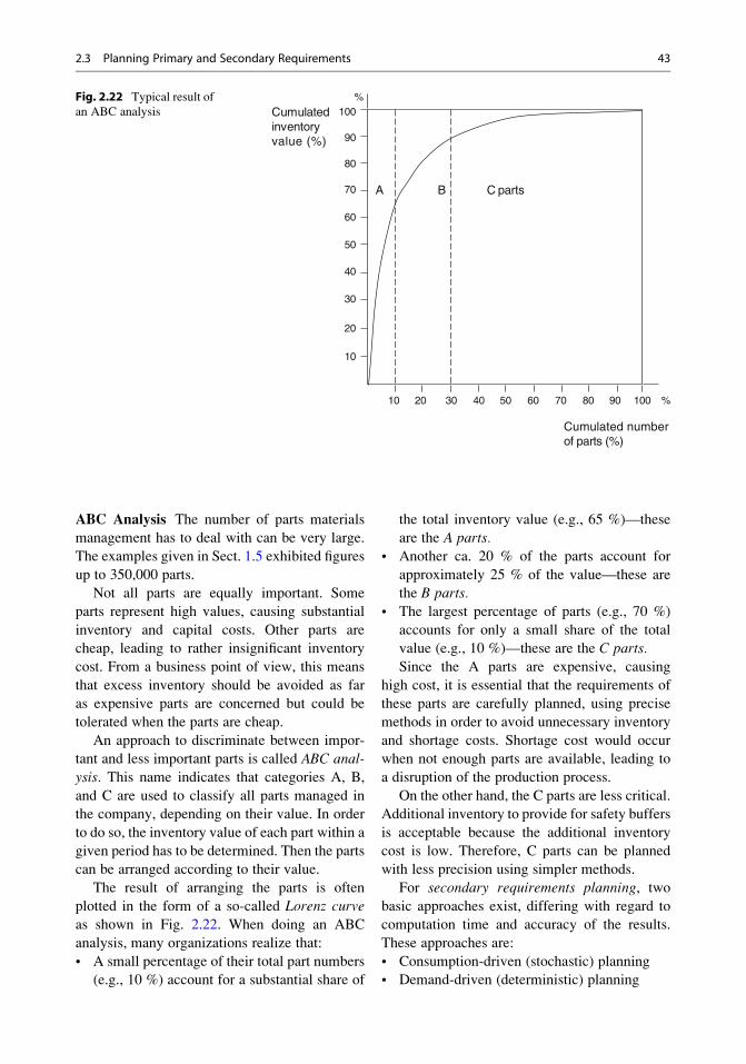
ABC Analysis The number of parts materials

management has to deal with can be very large.

The examples given in Sect. 1.5 exhibited figures

up to 350,000 parts.

Not all parts are equally important. Some

parts represent high values, causing substantial

inventory and capital costs. Other parts are

cheap, leading to rather insignificant inventory

cost. From a business point of view, this means

that excess inventory should be avoided as far

as expensive parts are concerned but could be

tolerated when the parts are cheap.

An approach to discriminate between impor-

tant and less important parts is called ABC anal-

ysis. This name indicates that categories A, B,

and C are used to classify all parts managed in

the company, depending on their value. In order

to do so, the inventory value of each part within a

given period has to be determined. Then the parts

can be arranged according to their value.

The result of arranging the parts is often

plotted in the form of a so-called Lorenz curveas shown in Fig. 2.22. When doing an ABC

analysis, many organizations realize that:

• A small percentage of their total part numbers

(e.g., 10 %) account for a substantial share of

the total inventory value (e.g., 65 %)—these

are the A parts.

• Another ca. 20 % of the parts account for

approximately 25 % of the value—these are

the B parts.

• The largest percentage of parts (e.g., 70 %)

accounts for only a small share of the total

value (e.g., 10 %)—these are the C parts.

Since the A parts are expensive, causing

high cost, it is essential that the requirements of

these parts are carefully planned, using precise

methods in order to avoid unnecessary inventory

and shortage costs. Shortage cost would occur

when not enough parts are available, leading to

a disruption of the production process.

On the other hand, the C parts are less critical.

Additional inventory to provide for safety buffers

is acceptable because the additional inventory

cost is low. Therefore, C parts can be planned

with less precision using simpler methods.

For secondary requirements planning, two

basic approaches exist, differing with regard to

computation time and accuracy of the results.

These approaches are:

• Consumption-driven (stochastic) planning

• Demand-driven (deterministic) planning

Cumulatedinventoryvalue (%)

Cumulated numberof parts (%)

A B C parts

100

90

80

70

60

50

40

30

20

10

%

10 20 30 40 50 60 70 80 90 100 %

Fig. 2.22 Typical result of

an ABC analysis

2.3 Planning Primary and Secondary Requirements 43


Consumption-driven planning is fairly simple

but not exact, whereas requirements-driven

planning is exact, but requires a lot of computing

effort. Taking these characteristics into account,

many companies choose to employ the two

approaches as follows:

• A parts are planned in a requirements-driven

way.

• B parts are also planned requirements driven

or partly requirements and partly consumption

driven.

• C parts are planned consumption driven.

2.3.1 Consumption-Driven Planning

Consumption-driven planning involves estimat-

ing the secondary requirements based on past

consumption rates, whereas requirements-driven

planning calculates the exact amounts using the

bills of materials.

The same methods used to forecast end-

product sales can be used to predict future mate-

rial requirements: moving averages, exponential

smoothing, etc. If the forecast value applies to an

entire period (e.g., a quarter) and consumption is

constant per unit of time, a consumption rate can

be calculated by dividing the forecast value by

the length of the period. This quotient is also

known as the withdrawal rate.

After the forecasted requirements have been

determined, two other issues need to be addressed:

1. When should a purchase order be placed

(for purchased parts) or a production order

be initiated (for in-house production)?

2. How much should be ordered or produced?

Both questions are interrelated. Shorter time

intervals between orders lead to smaller order

sizes and vice versa. In practice, the order date

is often determined by using the reorder point R.When the inventory falls below this level, an

order for a certain quantity (usually named Q)

is initiated. In inventory theory, this is referred to

as an (R, Q) policy (“reorder point/order-quantity

policy”).

Another order policy is the (s, S) policy, alsoknown as periodic review policy. In this policy,

two numbers, s and S, are used. When the

inventory is less than or equal to s, the difference

between a predefined maximum order quantity S

and the inventory on hand is ordered (Nahmias

2008, p. 263).

When using an (R, Q) policy, it is important to

set the reorder point high enough so that the

safety stock is preserved until the new order

arrives. The most important factor in determining

the reorder point is the replenishment time. It

includes (Mertens 2009, p. 76):

• Preparation time (preparation of a purchase

order or production order)

• Delivery time (for purchased parts) or lead

time (for in-house production)

• Storing time (time from goods received to

goods available for consumption)

The relationship between these times is

depicted in Fig. 2.23, assuming a linear decrease

in inventory. If tw represents the replenishment

time, then an order must be placed when the

stock level reaches R. The period of time tzserves as a buffer. Assuming the same constant

withdrawal rate, the production process will not

be affected by delivery delays shorter than tz.

The reorder point can be saved with the parts’

inventory or master data in the database, as long

as the withdrawal rate is more or less constant.

When a withdrawal is booked, the remaining

stock is compared with the reorder level. If the

remaining stock is below the reorder level, an

order is initiated. When there is a great deal of

fluctuation in the consumption, the reorder

level should not be maintained as a constant but

determined period by period to avoid unneces-

sary stock or shortages.

The risk of running short of inventory can to

some extent be countered with safety stock. It is

important to set the safety stock at an appropriate

level. A large safety stock means better protec-

tion from risk but leads to high inventory cost.

A small safety stock means less inventory cost

but a higher risk that missing material will

disrupt the manufacturing process. How much

safety stock is appropriate must therefore be

determined by balancing the cost of inventory

and the willingness to take risks.


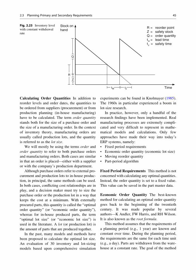
Calculating Order Quantities In addition to

reorder levels and order dates, the quantities to

be ordered from suppliers (procurement) or from

production planning (in-house manufacturing)

have to be calculated. The term order quantity

stands both for the size of a purchase order and

the size of a manufacturing order. In the context

of inventory theory, manufacturing orders are

usually called production lots, and the quantity

is referred to as the lot size.We will mostly be using the terms order and

order quantity to refer to both purchase orders

and manufacturing orders. Both cases are similar

in that an order is placed—either with a supplier

or with the company’s production department.

Although purchase orders refer to external pro-

curement and production lots to in-house produc-

tion, in principal, the same methods can be used.

In both cases, conflicting cost relationships are in

play, and a decision maker must try to size the

purchase order or the production lot in a way that

keeps the cost at a minimum. With externally

procured parts, this quantity is called the “optimal

order quantity” (or “economic order quantity”),

whereas for in-house produced parts, the term

“optimal lot size” (or “economic lot size”) is

used in the literature. A lot (or production lot) is

the amount of parts that are produced together.

In the past, many models and methods have

been proposed to calculate the optimal lot size.

An evaluation of 30 inventory and lot-sizing

models based upon comprehensive simulation

experiments can be found in Knolmayer (1985).

The 1960s in particular experienced a boom in

lot-size research.

In practice, however, only a handful of the

research findings have been implemented. Real

manufacturing processes are extremely compli-

cated and very difficult to represent in mathe-

matical models and calculations. Only few

approaches have made their way into today’s

ERP systems, namely:

• Fixed period requirements

• Economic order quantity (economic lot size)

• Moving reorder quantity

• Part-period algorithm

Fixed Period Requirements This method is not

concerned with calculating any optimal quantities.

Instead, the order quantity is set to a fixed value.

This value can be saved in the part master data.

Economic Order Quantity The best-known

method for calculating an optimal order quantity

goes back to the beginning of the twentieth

century. It was made popular by several

authors—K Andler, FW Harris, and RH Wilson.

It is also known as the root formula.This method assumes that the requirements of

a planning period (e.g., 1 year) are known and

constant over time. During the planning period,

the requirements are the same for each time unit

(e.g., a day). Parts are withdrawn from the ware-

house at a constant rate. The goal of the method

Q

Stock onhand

Time

R = reorder point Z = safety stockQ = order quantitytw = lead timetz = safety time

tW tZ

R

Z

Fig. 2.23 Inventory level

with constant withdrawal

rate


is to minimize the sum of the fixed and variable

(i.e., quantity dependent) costs within the

planning period. Variable cost is the cost depend-

ing on the size of the order, most of which is

inventory cost. Fixed cost is independent from

the order quantity. For in-house production, this

is primarily the setup cost.

Under the preconditions of this model, the

optimal order quantity is computed by minimiz-

ing a cost function. Let

Kl ¼ the total quantity dependent cost

Kr ¼ the total fixed cost in the planning

period

kl ¼ variable (quantity dependent) cost per

unit and period

kr ¼ fixed cost per order

a ¼ frequency of placing an order within the

planning period

T ¼ length of the planning period

y ¼ total demand in the planning period

x ¼ order quantity

Then the total fixed cost is

Kr ¼ akr

or, because a ¼ y/x,

Kr ¼ y=xkr:

Assuming a constant stock withdrawal rate,

the average stock is x/2, and thus, the total vari-

able cost amounts to

K1 ¼ x=2k1T:

Depending on the order quantity x, the total

decision relevant cost K is

KðxÞ ¼ Kr þ K1 ¼ y=xkr þ x=2k1T:

The minimum of this function, differentiated

by x, is

x¼ffiffiffiffiffiffiffiffiffi2kry

k1T

r:

x is the optimal order quantity (or “optimal lot

size,” “economic order quantity,” and “economic

lot size”). In order to meet the demand, xmust be

ordered a times within the planning period. From

a ¼ y/x follows

a¼ffiffiffiffiffiffiffiffiffiffiffiffiyk1T

2kr:

r

Although x is called an “optimal” order quan-

tity, this optimum can be achieved only under

restrictive premises, including the following:

• No capacity restrictions are in place regarding

the delivery (of externally procured parts),

production (of in-house produced parts), and

inventory capacities.

• The demand for the entire planning period is

known.

• The demand is the same for all periods. The

withdrawal rate is constant for all periods.

• The cost price (or the production cost, resp.)

per unit is given and independent of the quan-

tity.

• In the case of in-house production, the product

is not connected with other parts on higher or

lower manufacturing levels, or if so, these

connections can be disregarded.

Although in practice these premises are sel-

dom met, the root formula is still acknowledged

in inventory theory and remains one of the

options available in most ERP systems.

Moving Reorder Quantity Unlike the eco-

nomic order quantity, the moving reorder-quantity

(MRQ) method does not assume that the demand

is the same for all (sub) periods across the entire

planning horizon. Instead, different demand

values per period are considered.

The MRQmethod approximates the minimum

of the total cost per unit. For a single demand yito be met in period j, which is procured or

produced in period i (i � j), the inventory cost

for storing the quantity yi amounts to

k1yj j� ið Þ:


Combining the demands of the periods i to

t (i � t) into one order results in inventory cost of

k1Xt

j¼i

yj j� ið Þ:

The total cost of periods i to t, Kit, is then

kit ¼ kr þ k1Xt

j¼i

yj j� ið Þ:

and the cost per unit is

kit ¼ kitPtj¼i

yj

:

The moving reorder-quantity method pro-

ceeds step by step, adding up period demands

one by one until kit has reached its minimum. In

other words, we are looking for that value of t for

which

kit<kitþ1

if one more demand (yt + 1) were added. Once the

value of t has been determined, the optimal order

quantity is

x ¼Xt

j¼i

yj:

The moving reorder-quantity method is suit-

able in practice when the demands of all periods

and the cost coefficients kr and k1 are known. It

does, however, have the disadvantage that mini-

mizing the cost per unit is not necessarily the

same as minimizing the total cost of a planning

period.

Part-Period Algorithm The part-period algo-

rithm attempts to minimize the cost per order

(DeMatteis 1968). It builds on a property of the

classical economic order-quantity model, nam-

ely, that in the optimum, the inventory cost

K1 and the fixed cost Kr are equal. This can be

seen by setting the first derivative of the cost

function

KðxÞ ¼ y=x � kr þ x=2 � k1T

to zero, resulting in

y=x � kr ¼ x=2 � k1T:

The left side of the equation has the fixed cost

Kr, while the right side has the inventory cost K1.

The part-period algorithm applies this

property to a situation where the demand is not

continuous, as in the economic lot-size model,

but discrete (i.e., individual period demands).

In the part-period algorithm, the optimum is

approximately reached when an order’s inven-

tory cost equals its fixed cost:

k1Xt

j¼i

yj j� ið Þ ¼ kr

A transformation of this equation to

Xt

j¼i

yj j� ið Þ ¼ krk1

shows that both sides have the dimension “quan-

tity multiplied by periods” (or “number of partsmultiplied by number of periods”), hence the

name of this method.

Just as in the moving reorder-quantity

method, the algorithm proceeds by successively

adding period demands yt and examining

whether or not the left side is still less than the

right. Once

k1Xtþ1

j¼i

yj j� ið Þ>kr;

the optimum has been passed. Hence, the optimal

order quantity is

x ¼Xt

j¼i

yj:


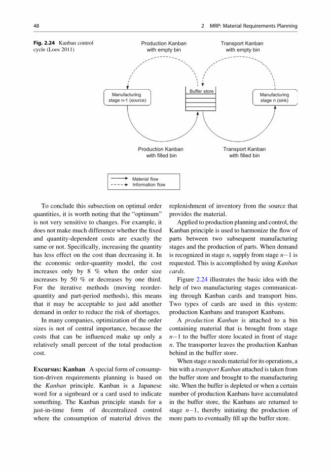
To conclude this subsection on optimal order

quantities, it is worth noting that the “optimum”

is not very sensitive to changes. For example, it

does not make much difference whether the fixed

and quantity-dependent costs are exactly the

same or not. Specifically, increasing the quantity

has less effect on the cost than decreasing it. In

the economic order-quantity model, the cost

increases only by 8 % when the order size

increases by 50 % or decreases by one third.

For the iterative methods (moving reorder-

quantity and part-period methods), this means

that it may be acceptable to just add another

demand in order to reduce the risk of shortages.

In many companies, optimization of the order

sizes is not of central importance, because the

costs that can be influenced make up only a

relatively small percent of the total production

cost.

Excursus: Kanban A special form of consump-

tion-driven requirements planning is based on

the Kanban principle. Kanban is a Japanese

word for a signboard or a card used to indicate

something. The Kanban principle stands for a

just-in-time form of decentralized control

where the consumption of material drives the

replenishment of inventory from the source that

provides the material.

Applied to production planning and control, the

Kanban principle is used to harmonize the flow of

parts between two subsequent manufacturing

stages and the production of parts. When demand

is recognized in stage n, supply from stage n�1 is

requested. This is accomplished by using Kanban

cards.

Figure 2.24 illustrates the basic idea with the

help of two manufacturing stages communicat-

ing through Kanban cards and transport bins.

Two types of cards are used in this system:

production Kanbans and transport Kanbans.

A production Kanban is attached to a bin

containing material that is brought from stage

n�1 to the buffer store located in front of stage

n. The transporter leaves the production Kanban

behind in the buffer store.

When stage n needsmaterial for its operations, a

bin with a transport Kanban attached is taken from

the buffer store and brought to the manufacturing

site. When the buffer is depleted or when a certain

number of production Kanbans have accumulated

in the buffer store, the Kanbans are returned to

stage n�1, thereby initiating the production of

more parts to eventually fill up the buffer store.

Production Kanbanwith empty bin

Production Kanbanwith filled bin

Transport Kanbanwith empty bin

Transport Kanbanwith filled bin

Manufacturing stage n-1 (source)

Manufacturing stage n (sink)

Material flowInformation flow

Buffer store

Fig. 2.24 Kanban control

cycle (Loos 2011)


In case stage n�1 runs short of parts needed

for the production, demand is communicated to

stage n�2, using the production Kanbans in the

buffer store in the front of stage n�1. This

continues all the way to the raw-material stage.

In this fashion, the entire manufacturing chain,

from the last stage to the first, is organized

according to the “pull principle,” demanding

supply when it is actually needed.

Conventional MRP and MRP II planning, on

the other hand, relies on the “push principle,”

meaning that supply is provided to stage n by

stage n-1 according to previously planned

demand and not to actual demand.

Kanban was originally developed by Toyota as

a manual approach to lean production (Ohno and

Bodek 1988). Meanwhile, electronic versions

have been implemented in a number of ERP

systems, sometimes called “e-Kanban.” Instead

of paper cards, they employ electronic media

using barcodes or RFID tags (cf. Sect. 11.4.1).

Kanban works best when the flow of produc-

tion is smooth and uninterrupted, as can be the

case in series or mass production. Kanban is

actually a means of fine-tuning smooth produc-

tion. Conditions under which the Kanban

approach has proved to be beneficial include the

following (Takeda 2006, pp. 185–189):

• Standardized production program, using

standard parts as much as possible in order

to realize continuous consumption

• Production organization according to the

material flow

• Effective transportation system, short trans-

port times

• Small lots (lot size is in fact the amount of

parts that fit into one or more bins)

• High availability of operating facilities, short

changeover times

• Low defect rate through immediate quality

assurance at the workplace

Kanban systems exist in different versions and

are used for different purposes. Some applica-

tions utilize more or fewer types of Kanbans

instead of the two described above. This is the

case when external suppliers are included. The

most successful applications of Kanban have

been reported from supply chains of the Japanese

automotive industry.

2.3.2 Requirements-Driven Planning

While consumption-driven planning focuses on

assumptions and estimates, requirements-driven

planning is based on certainty. Therefore, it is

also called deterministic planning. As long as

the primary requirements are as expected, the

secondary requirements can be calculated

exactly. For this purpose, product structures

(bills of materials) are employed to determine

the quantities of subordinate parts needed to

produce the primary requirements.

Using bills ofmaterials to determine the second-

ary requirements is also known as bill of materials

explosion. Programs exploding bills of materials

are called bill of materials processors (BOM

processors). A BOM processor is a core compo-

nent of any MRP system.

Whereas consumption-driven planning treats

each part separately, requirements-driven planning

must take into account how the parts are related

with each other. Because of the hierarchical rela-

tionships within the product structures, decisions

made on a higher level affect the lower levels as

well.

When in Fig. 2.25, for example, the lot size of

assembly A is doubled, the secondary require-

ments for parts that go into this assembly

(D and E) are also doubled. On the other hand,

if assembly C is still stocked, less of C needs to

be produced and also less of all other parts

that go directly or indirectly into C (i.e., G, H,

I, and J).

This example clearly shows that in require-

ments-driven planning, calculating gross and net

requirements and building lot sizes are closely

connected. Principally, each of the following

tasks must be completed for every part, before

the next part is dealt with:

1. Gross requirements planning

2. Net requirements planning

3. Order-size planning

4. Dependent requirements planning


5. Forward shifting

When dealing with a leaf of a product struc-

ture tree, the last two tasks are omitted.

Gross Requirements Planning For end pro-

ducts and sellable intermediate products, planning

the gross requirements starts from the primary

requirements as determined in primary require-

ments planning (cf. Sect. 2.3.1). For dependent

parts, the starting point is the secondary require-

ments derived from higher-level nodes of the prod-

uct hierarchy. In addition to these quantities, other

components may be added, for example, require-

ments for replacement parts and estimates based

on seasonal consumption patterns.

Net Requirements Planning To determine the

net requirements, available stock must be sub-

tracted from the gross requirements. Parts

planned according to the requirements-driven

approach may still be stocked, for example,

when inventory orders were included in the

plan (i.e., internal orders filling gaps in the capac-

ity utilization), when the gross requirements

include consumption-driven components, or

when unneeded buffers are left over (e.g., for a

previous order, more than the actually needed

quantity was produced).

Depending on how differentiated the ware-

housing structure is, safety stock, shop-floor

stock, reservations, and open purchase orders

may be taken into consideration. If waste is

anticipated, the net requirements must be

multiplied by the expected waste factor.

A detailed scheme for planning gross and net

requirements is shown in Fig. 2.26 (Mertens

2009, p. 133). It contains sample data for

the above-mentioned factors, divided into

periods.

Order-Size Planning When the net require-

ments for a certain number of periods are

known, they can either be directly used for

planning the requirements on the next level or

they can be bundled into production lots. In

Fig. 2.26, the net requirements from periods 2,

3, and 4 have been combined into one lot (2,208

units) and the net requirements from periods 5

and 6 into another lot (1,887 units).

Order quantities may also be computed

for externally procured parts. However, the steps

following order-size planning—derived require-

ments planning and forward shifting—are obvi-

ously not applicable to purchased parts. Instead,

purchase orders are created and order placement is

initiated.

For lot-size planning, basically the same

methods as described above are used. From a

theoretical standpoint, this is problematic

because the presumptions on which the

“optimality” of a lot size is based are largely

not met. In particular, computing lot sizes with-

out considering the connections with other parts

can cause problems later on. The quantity of a lot

on a given level of a product structure affects the

planning of all parts on the lower levels. This

problem will be explored in more detail with the

help of Figs. 2.27 and 2.28 below.

Dependent Requirements Planning This pro-

cess step starts from the production lots com-

puted in step 3. Using the product structures of

the parts involved, it derives dependent (or sec-

ondary) requirements. Multiplying the lot size

with the quantity coefficients results in the quan-

tities of those parts directly needed for the cur-

rent part.

As an example, let us assume that the

planning shown in Fig. 2.26 was for assembly C

X

A C

D E G

JI

2 1 2

2 1 4

2 4

2 1

B

F H

Fig. 2.25 Product structure (example)


Period 1 2 3 4 5 6

Total dependent requirements for one assembly (from BOM explosion) 700 550 1300 800 900 700

+ Consumption-driven demand 270 400 300 140 340 250

+ Independent requirements (replacements) 130 200 100 60 160 50

= Gross requirements 1100 1150 1700 1000 1400 1000

Warehouse stock 3000 - Safety stock 300- Reserved stock*) 900

= Available stock 1800 1800 700 300 600

Open production-order quantity 900 - Forecasted rejections 90

- Inflow from recycling 50 100

= Available stock from production order 810 450 360

= Net requirements - 400 1250 340 700 1000

+ Additional requirements for scrap (10%, factor 0.11) - 44 137 37 77 110

= Extended net requirements - 444 1387 377 777 1110

Lot sizing - 2208 - - 1887 -

*) This reserved stock is released to Exact requirements for further planning/explosion available stock in periods 4 and 5.

Fig. 2.26 Gross and net

requirements planning

[Mertens 2009, p. 133]

Period 1 2 3 4 5 6

Net requirements C(after lot-size planning)

- 2208 - - 1887 -

Dependent requirements G - 4416 - - 3774 -

After forward shifting 4416 - - 3774 - -

Dependent requirements H - 2208 - - 1887 -

After forward shifting 2208 - - 1887 - -

Fig. 2.27 Derived

requirements and forward

shifting with lot sizes

Period 1 2 3 4 5 6

Net requirements C(no lot sizing)

- 444 1387 377 777 1110

Dependent requirements G - 888 2774 754 1554 2220

After forward shifting 888 2774 754 1554 2220 -

Dependent requirements H - 444 1387 377 770 1110

After forward shifting 444 1387 377 777 1110 -

Fig. 2.28 Derived

requirements and forward

shifting without lot sizes


of Fig. 2.25. Figure 2.27 continues the planning

process, illustrating the dependent requirements

for parts G and H.

Forward Shifting Although the focus of MRP

is on planning quantities, the temporal structure

of the production process is not completely dis-

regarded. Taking into account that executing a

production order takes a certain amount of time,

the derived requirements needed for the order

must be completed earlier by just that amount

of time. This time is called a forward shift or

lead-time offset. If, for example, the size of lot C

is such that it takes 14 days to manufacture the

lot, then all parts that go into C (H and G) must be

available 14 days earlier than C, that is, the lead-

time offset is 14 days.

The purpose of forward shifting is to give the

material requirements plan a rough temporal

structure. This, however, is not straightfor-

ward, because the actual manufacturing dates

depend on decisions that are made later in the

planning process. Therefore, rough estimates

based on experience have to be used instead,

depending on what information is available,

how certain the expectations are, and how much

computational effort is reasonable. Typical

approaches are:

• The lead time is actually calculated, using the

setup, transition, and processing times

stored in the routing and operating facility

data. This time is then used to shift the

derived requirements forward (i.e., toward

the present).

• The same forward shift is applied across the

board for all parts of one manufacturing level.

The lead-time offset can be determined, for

example, from the average offset that was

actually observed in the past.

• The same forward shift (e.g., one or two

periods) is applied to all parts and all

manufacturing levels.

The first approach is without question the

most accurate, provided that the lead-time

components can be predicted with sufficient

certainty. Unfortunately, calculating a for-

ward shift is often not feasible, because it

would basically require a complete lead-time

and capacity-scheduling run. Therefore, many

manufacturing companies use the same time

span as lead-time offset for all parts of the

same manufacturing level or even across all

levels. The schema of Fig. 2.27 showed an

example of a standard lead-time offset of

one period.

When all steps of requirements-driven

planning for the part under consideration have

been completed, the same steps are applied to

the next part, as long as the part is not a leaf of a

product structure tree. In this way, roughly sched-

uled derived requirements are created for all

parts. In one of the next rounds, for example, the

tasks of gross and net requirements planning,

lot-size planning, dependent requirements

planning, and forward shifting will be executed

for assembly G.

Impact of Lot-Size Planning When individual

requirements on a higher level are bundled into

lots, this changes the requirements and time

planning of all lower parts, directly or indirectly.

To demonstrate the effect of lot sizing, we will

take up the planning scheme shown in Fig. 2.26.

If each period’s requirement is produced as a

separate lot (i.e., no specific lot sizing), the

derived quantities and dates for parts G and H

are as in Fig. 2.28, assuming a forward shift of one

period. If, however, lots are planned, require-

ments for lower-level parts going into the current

part move up in time. The required quantities are

higher in some periods and nonexistent in others.

This effect was illustrated in Fig. 2.27.

Another effect of lot-size planning is that

assumptions are made regarding the availability

of the operating facilities at the implied manu-

facturing dates. Not only the facilities needed

for the current part but also those needed for the

subordinate parts have to be available on the

right dates so that the production can be

completed on time.

To illustrate this effect, let us assume that part

H needs only one machine and the capacity

requirements are approximately proportional to

the quantity. In this case, the allocation of


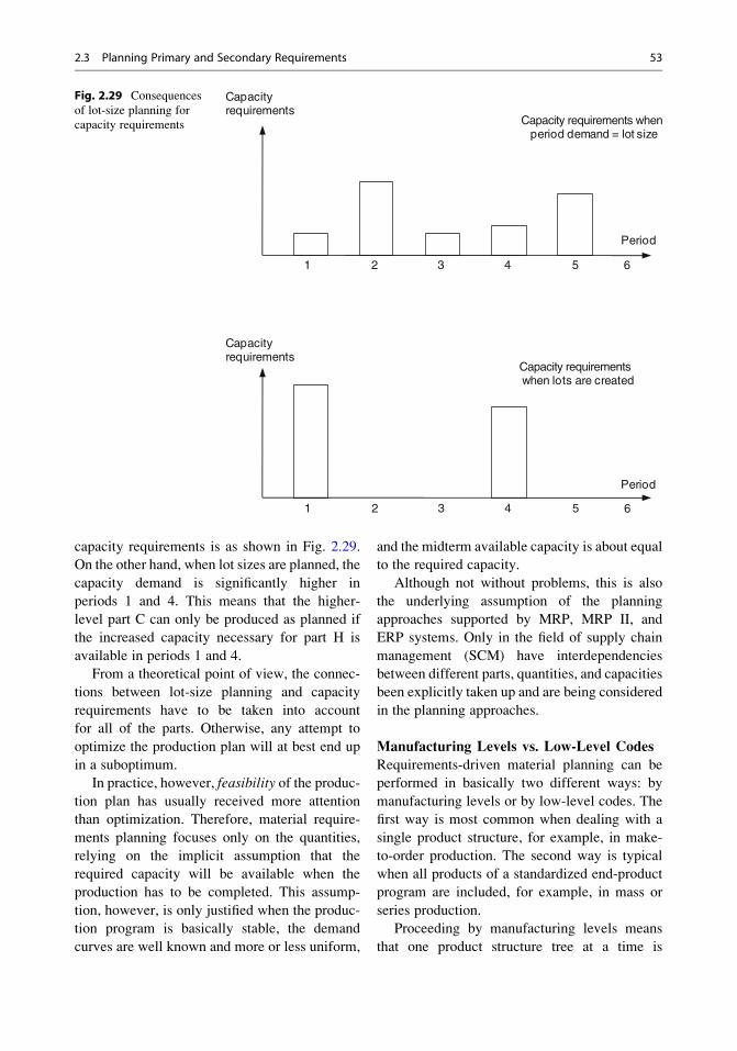
capacity requirements is as shown in Fig. 2.29.

On the other hand, when lot sizes are planned, the

capacity demand is significantly higher in

periods 1 and 4. This means that the higher-

level part C can only be produced as planned if

the increased capacity necessary for part H is

available in periods 1 and 4.

From a theoretical point of view, the connec-

tions between lot-size planning and capacity

requirements have to be taken into account

for all of the parts. Otherwise, any attempt to

optimize the production plan will at best end up

in a suboptimum.

In practice, however, feasibility of the produc-

tion plan has usually received more attention

than optimization. Therefore, material require-

ments planning focuses only on the quantities,

relying on the implicit assumption that the

required capacity will be available when the

production has to be completed. This assump-

tion, however, is only justified when the produc-

tion program is basically stable, the demand

curves are well known and more or less uniform,

and the midterm available capacity is about equal

to the required capacity.

Although not without problems, this is also

the underlying assumption of the planning

approaches supported by MRP, MRP II, and

ERP systems. Only in the field of supply chain

management (SCM) have interdependencies

between different parts, quantities, and capacities

been explicitly taken up and are being considered

in the planning approaches.

Manufacturing Levels vs. Low-Level Codes

Requirements-driven material planning can be

performed in basically two different ways: by

manufacturing levels or by low-level codes. The

first way is most common when dealing with a

single product structure, for example, in make-

to-order production. The second way is typical

when all products of a standardized end-product

program are included, for example, in mass or

series production.

Proceeding by manufacturing levels means

that one product structure tree at a time is

Capacityrequirements

621 3 4 5

Period

Capacity requirements whenperiod demand = lot size

621 3 4 5

Period

Capacityrequirements

Capacity requirementswhen lots are created

Fig. 2.29 Consequences

of lot-size planning for

capacity requirements


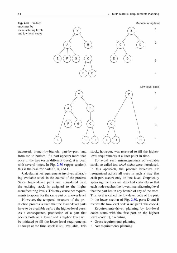
traversed, branch-by-branch, part-by-part, and

from top to bottom. If a part appears more than

once in the tree (or in different trees), it is dealt

with several times. In Fig. 2.30 (upper section),

this is the case for parts C, D, and E.

Calculating net requirements involves subtract-

ing available stock in the course of the process.

Since higher-level parts are considered first,

the existing stock is assigned to the higher

manufacturing levels. This may cause net require-

ments to appear for the same part on a lower level.

However, the temporal structure of the pro-

duction process is such that the lower-level parts

have to be available before the higher-level parts.As a consequence, production of a part that

occurs both on a lower and a higher level will

be initiated to fill the lower-level requirements,

although at the time stock is still available. This

stock, however, was reserved to fill the higher-

level requirements at a later point in time.

To avoid such misassignments of available

stock, so-called low-level codes were introduced.

In this approach, the product structures are

reorganized across all trees in such a way that

each part occurs only on one level. Graphically

speaking, the trees are stretched vertically so that

each node reaches the lowest manufacturing level

that the part has in any branch of any of the trees.

This level is called the low-level code of the part.

In the lower section of Fig. 2.30, parts D and E

receive the low-level code 4 and part C the code 4.

Requirements-driven planning by low-level

codes starts with the first part on the highest

level (code 1), executing:

• Gross requirements planning

• Net requirements planning

Y

A B

E

GF C

Z

D

C

Manufacturing level

Y

A B

E GF C

DE

Z

C

DE

D

1

4

3

2

1

2

3

Low-level code

4DE DE

Fig. 2.30 Product

structures by

manufacturing levels

and low-level codes


• Lot-size planning

• Deriving requirements for subordinate parts

• Forward shifting

for this part. Then it continues with the next part

of level 1, then with the next to the next part of

level 1, etc. When all parts of level 1 have been

dealt with, the process goes to the next level,

treating all parts with low-level code 2 as

above, then to the next level, etc.

In this process, requirements for subordinate

parts occurring on several levels and/or in several

product structures are gradually collected and

accumulated, as the process touches the respec-

tive nodes in those structures. Requirements

planning for a derived part (i.e., gross and net

requirements planning, lot sizing, etc.) does not

start until the part’s low-level code has been

reached in the process. When all parts on all

levels have been dealt with, the total require-

ments for all parts are available in the database.

Using low-level codes, the parts shown in

Fig. 2.30 would be processed in the following

sequence:

Level 1: Y, Z

Level 2: A, B

Level 3: C, F, G

Level 4: D, E

Low-level codes help to avoid mistakes in

requirements-driven planning such as inadequate

allocation of stock, but they also have disadvan-tages. Worth mentioning is the administration

effort. Creating the codes across hundreds of

thousands or millions of parts is an extremely

time-consuming task, although simple from an

algorithmic point of view. Basically, it involves

traversing all product structure trees and for each

part, storing the lowest manufacturing level ever

reached in the part master record.

More problematic than the one-time creation

is the maintenance effort. Every time a new part

Y

A B

E GF S

Z

D

S

b C is replaced by S

a Z is extended by P Low-level code

Y

A B

E

G

F

C

DE F

Q

P

Z

C

DE D

1

4

3

2

1

2

3

Fig. 2.31 Induced changes of low-level codes


is entered into the database, its low-level code

must be determined, but what is worse, the codes

of all other parts in the database must be reeval-

uated. The reason is that the codes may need to

be changed due to the product structure of the

new part. The same applies when an existing part

is deleted from the database.

Figure 2.31 illustrates the two scenarios. The

top section of the figure shows the case that end

product Z is augmented by part P. Part F goes

into part Q, which goes into P. Part F was already

contained in the product structure of end product

Y (with low-level code 3). Introducing P changes

the low-level code of F to 4 because in Z’s

product structure, F is on a lower manufacturing

level than in Y’s.

The lower section of the figure shows a sce-

nario in which assembly C is no longer produced

in-house but replaced with a purchased part S.

Since C is not there anymore, D and E are not

needed either (for C) but are still needed for Z

and A, respectively. They move up according to

Y’s and Z’s product structures, and their low-

level codes are now equal to the manufacturing

levels.

2.3.3 MRP in Make-to-OrderProduction

An essential characteristic of make-to-order pro-

duction is that the product is specific to the cus-

tomer. This means that important master data such

as product structures may not be available and

have to be created for the order. Furthermore,

customer-specific products are not produced to

stock but only when the customer places an

order. This is actually an expensive strategy in

comparison tomass or series production. The com-

pany cannot benefit from cost savings that go

along with larger batches if they produce only

customer-specific parts. Likewise, it is difficult to

meet short delivery dates if for all parts, planning

can only start when a customer order is placed.

For these reasons, make-to-order manufac-

turers strive to use not only customer-specific

parts but also standard parts where possible.

Since standard parts are typically included in

more than one product, they can be planned

independently from specific customer orders

and produced in larger batches, which saves

time and cost.

Planning Levels Different planning levels can

be introduced to handle customer-specific parts

and standard parts. Zimmermann called these

levels the expectation-oriented planning level

and the customer-order-oriented planning level

(Zimmermann 1989, pp. 74–76).

Figure 2.32 illustrates this distinction with the

help of two product structures representing the

customer-specific products Y and Z. The com-

pany has decided to use the standard parts C, E,

and F whenever possible, but A, B, D, and G

are parts that must be manufactured just for the

customer order.

As the figure shows, planning for the parts Y,

Z, A, B, D, and G will be done when a customer

order arrives, while planning for the parts C, E,

and F can be done whenever suitable, for exam-

ple, following a consumption-driven approach as

described in Sect. 2.3.1. The dashed line between

the two planning levels is called the stock-

keeping level.

Inventory management in make-to-order

production has to meet more challenges than

in make-to-stock production. The reason is that

consumption is not as smooth as in make-to-stock

production where the planning can be based on a

known, possibly constant withdrawal rate. In

make-to-order production, the future customer

orders are not known, and hence, derived require-

ments can at best only be estimated. Consequently,

higher inventory levels including safety buffers

have to be kept, causing additional inventory cost.

Alternatively, the company may try to keep

the inventory (for standard parts) at a reasonably

low level and purchase peak demand from sup-

pliers or competitors. In some industries, for

example, suppliers exist that have specialized in

express delivery of certain materials at substan-

tially increased prices (e.g., special materials

which otherwise have long delivery times). If

such an option is available, the company may

consider a trade-off between increasing the

inventory level (i.e., high inventory cost) and


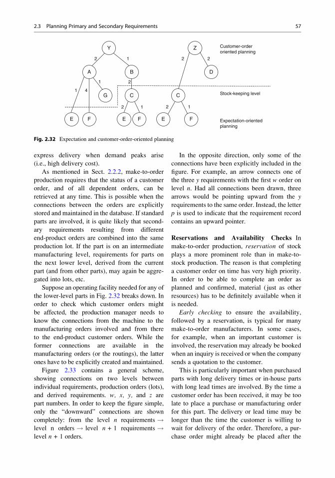
express delivery when demand peaks arise

(i.e., high delivery cost).

As mentioned in Sect. 2.2.2, make-to-order

production requires that the status of a customer

order, and of all dependent orders, can be

retrieved at any time. This is possible when the

connections between the orders are explicitly

stored and maintained in the database. If standard

parts are involved, it is quite likely that second-

ary requirements resulting from different

end-product orders are combined into the same

production lot. If the part is on an intermediate

manufacturing level, requirements for parts on

the next lower level, derived from the current

part (and from other parts), may again be aggre-

gated into lots, etc.

Suppose an operating facility needed for any of

the lower-level parts in Fig. 2.32 breaks down. In

order to check which customer orders might

be affected, the production manager needs to

know the connections from the machine to the

manufacturing orders involved and from there

to the end-product customer orders. While the

former connections are available in the

manufacturing orders (or the routings), the latter

ones have to be explicitly created and maintained.

Figure 2.33 contains a general scheme,

showing connections on two levels between

individual requirements, production orders (lots),

and derived requirements. w, x, y, and z are

part numbers. In order to keep the figure simple,

only the “downward” connections are shown

completely: from the level n requirements !level n orders ! level n + 1 requirements !level n + 1 orders.

In the opposite direction, only some of the

connections have been explicitly included in the

figure. For example, an arrow connects one of

the three y requirements with the first w order on

level n. Had all connections been drawn, three

arrows would be pointing upward from the y

requirements to the same order. Instead, the letter

p is used to indicate that the requirement record

contains an upward pointer.

Reservations and Availability Checks In

make-to-order production, reservation of stock

plays a more prominent role than in make-to-

stock production. The reason is that completing

a customer order on time has very high priority.

In order to be able to complete an order as

planned and confirmed, material ( just as other

resources) has to be definitely available when it

is needed.

Early checking to ensure the availability,

followed by a reservation, is typical for many

make-to-order manufacturers. In some cases,

for example, when an important customer is

involved, the reservation may already be booked

when an inquiry is received or when the company

sends a quotation to the customer.

This is particularly important when purchased

parts with long delivery times or in-house parts

with long lead times are involved. By the time a

customer order has been received, it may be too

late to place a purchase or manufacturing order

for this part. The delivery or lead time may be

longer than the time the customer is willing to

wait for delivery of the order. Therefore, a pur-

chase order might already be placed after the

Y

A B

E

G

F

C

FE

2 1

1 4

2 1

2

Z

C

D

E F

2 2

2 1

1

Customer-orderoriented planning

Stock-keeping level

Expectation-orientedplanning

Fig. 2.32 Expectation and customer-order-oriented planning


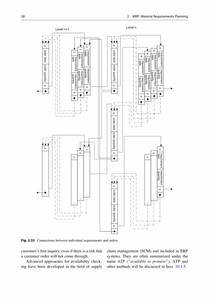
customer’s first inquiry, even if there is a risk that

a customer order will not come through.

Advanced approaches for availability check-

ing have been developed in the field of supply

chain management (SCM) and included in ERP

systems. They are often summarized under the

name ATP (“available to promise”). ATP and

other methods will be discussed in Sect. 10.1.5.

Level nLevel n+1

wp

order dateorder quantity




p

pp

w

y

x

requirement

daterequirem

entquantity

wp

requirement

daterequirem

entquantity

wp

requirement

daterequirem

entquantity

wp

requirement

daterequirem

entquantity

wp

requirement

daterequirem

entquantity

px

x

x

requirement

daterequirem

entquantity

yp

requirement

daterequirem

entquantity

yp

requirement

daterequirem

entquantity

yp

z

z

z

z

Fig. 2.33 Connections between individual requirements and orders



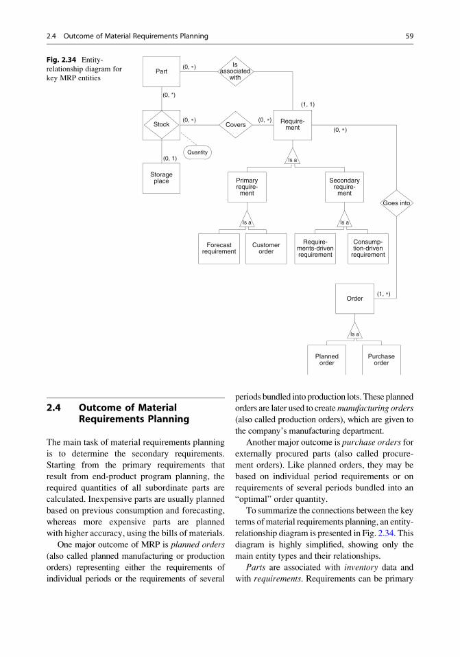
2.4 Outcome of MaterialRequirements Planning

The main task of material requirements planning

is to determine the secondary requirements.

Starting from the primary requirements that

result from end-product program planning, the

required quantities of all subordinate parts are

calculated. Inexpensive parts are usually planned

based on previous consumption and forecasting,

whereas more expensive parts are planned

with higher accuracy, using the bills of materials.

One major outcome of MRP is planned orders

(also called planned manufacturing or production

orders) representing either the requirements of

individual periods or the requirements of several

periods bundled into production lots. These planned

orders are later used to createmanufacturing orders

(also called production orders), which are given to

the company’s manufacturing department.

Another major outcome is purchase orders for

externally procured parts (also called procure-

ment orders). Like planned orders, they may be

based on individual period requirements or on

requirements of several periods bundled into an

“optimal” order quantity.

To summarize the connections between the key

terms ofmaterial requirements planning, an entity-

relationship diagram is presented in Fig. 2.34. This

diagram is highly simplified, showing only the

main entity types and their relationships.

Parts are associated with inventory data and

with requirements. Requirements can be primary

Stock

PartIs

associatedwith

Covers

Storageplace

Is aQuantity

Require-ment

Is a

Primaryrequire-

ment

Is a

Secondaryrequire-

ment

Customerorder

Forecastrequirement

Consump-tion-driven

requirement

Require-ments-drivenrequirement

Goes into

Is a

Order

Purchaseorder

Plannedorder

(0, )

(0, *)

(0, ) (0, )

(0, )

(0, 1)

(1, )

(1, 1)

Fig. 2.34 Entity-

relationship diagram for

key MRP entities

2.4 Outcome of Material Requirements Planning 59

or secondary requirements. Primary requirements

come from forecasts or from customer orders.

Secondary requirements are computed as either

consumption driven or requirements driven.

To be satisfied, requirements on all levels

finally have to go into orders, which can be

planned orders (for in-house production) or

purchase orders (for external procurement).


http://www.springer.com/978-3-642-31572-5

mrp: material requirements planning 2 - fac.ksu.edu.safac.ksu.edu.sa/sites/default/files/mrp-...

Documents