mri noise estimation and denoising using non-local pca
TRANSCRIPT

1
MRI noise estimation and denoising
using non-local PCA
José V. Manjóna, Pierrick Coupéb, Antonio Buadesc
[email protected], [email protected], [email protected]
a Instituto de Aplicaciones de las Tecnologías de la Información y de las Comunicaciones
Avanzadas (ITACA), Universidad Politécnica de Valencia, Camino de Vera s/n, 46022 Valencia,
Spain
b Laboratoire Bordelais de Recherche en Informatique, Unité Mixte de Recherche CNRS (UMR
5800), PICTURA Research Group, 351, cours de la Libération F-33405 Talence cedex, France.
c Dpt Matemàtiques i Informàtica, Universitat Illes Balears, Ctra Valldemossa km 7.5, 07122
Palma de Mallorca, Spain.
* Corresponding author: José V. Manjón. Instituto de Aplicaciones de las Tecnologías de la
Información y de las Comunicaciones Avanzadas (ITACA), Universidad Politécnica de Valencia,
Camino de Vera s/n, 46022 Valencia, Spain
Tel.: (+34) 96 387 70 00 Ext. 75275, Fax: (+34) 96 387 90 09
E-mail: [email protected] (José V. Manjón)
Keywords: MRI, PCA, denoising, sparseness, non-local means
Abbreviations:
PCA: Principal Component Analysis
NLM: Non Local Means
PSNR: Peak signal to Noise Ratio
RMSE: Root mean squared error
SSIM: Structural similarity index

2
Abstract
This paper proposes a novel method for MRI denoising that exploits both the sparseness and
self-similarity properties of the MR images. The proposed method is a two-stage approach that
first filters the noisy image using a non local PCA thresholding strategy by automatically
estimating the local noise level present in the image and second uses this filtered image as a
guide image within a rotationally invariant non-local means filter. The proposed method
internally estimates the amount of local noise presents in the images that enables applying it
automatically to images with spatially varying noise levels and also corrects the Rician noise
induced bias locally. The proposed approach has been compared with related state-of-the-art
methods showing competitive results in all the studied cases.

3
1. Introduction
Magnetic resonance (MR) imaging has very important role on current medical and research
procedures. However, these images are inherently noisy and thus filtering methods are required
to improve the data quality. This denoising process is usually performed as a preprocessing
step in many image processing and analysis tasks such as registration or segmentation.
There is a large amount of bibliography related to the denoising topic that highlights the
relevance of this issue for the scientific community. A large review of MRI denoising methods
can be found at Mohan et al (2014). Currently, most denoising methods can be classified on
those that use the intrinsic pattern redundancy of the data and those exploiting their sparseness
properties.
On the first class, the well known non-local means (NLM) filter (Buades et al,2005) is maybe the
most representative method. This method reduces the noise by exploiting the self-similarity of
the image patterns by averaging similar image patterns. In MRI, early works using the NLM
method are from Coupe et al (2008) and Manjón et al (2008). The bibliography related to this
method is quite extensive (Tristan-Vega et al, 20012; Coupe et al., 2012; Manjón et al., 2009,
2010, 2012; Wiest-Daesslé et al, 2008; He and Greenshields, 2009; Rajan et al. 2012, 2014).
On the other hand, sparseness-based methods try to reduce the noise naturally present in the
images by assuming that the noisy data can be represented in a lower dimensionality space. In
such methods, it is considered that most of the signal can be sparsely represented using few
bases that enables to discard the noise related components or simply approximate noisy
patterns by their corresponding noise free patterns. An example of these techniques are for
instance those based on FFT or DCT transforms where standard bases such as sin or cosine
functions are used to represent the images (Guleryuz, 2003; Yaroslavsky et al., 2000). In this
case, noise reduction is achieved by removing noise related coefficients in a transform domain
using either soft or hard thresholding techniques. More recently, techniques that learn the bases
from the images to be denoised have received much attention (Elad et al. 2006, Mairal et
al.,2008; Protter et al.,2009). These techniques learn a set of bases from the images to be
denoised or from a set of similar noise free images to create a dictionary to sparsely represent
image patches as a linear combination of dictionary entries (Aharon et al. 2006). The advantage
of these dictionaries over standard ones such those used on DCT or FFT transforms is the fact
they are better adapted to the images to be processed that enables a sparser representation
and therefore a better signal/noise separation. In MRI, sparse theory has been used in many
recent methods (Bao et al.2008; Bao et al. 2013; Pattel et al.2011).
Principal Component Analysis (PCA) and related approaches have been also used for noise
reduction in images (Muresan et al., 2003; Bydder et al., 2003; Deledalle et al., 2011). This type
of technique falls in the second category since it takes benefit from the fact that original signal
can be projected into an orthogonal space where most of the variance of the signal is

4
accumulated in few components while the noise being not sparse is uniformly spread over all
the components. Noise reduction using PCA normally requires 3 main steps: 1) decomposing a
set of selected signals into their principal components, 2) shrinking noise related components,
and finally 3) reconstructing back the signals by inverting the PCA decomposition. This
approach was first used by Muresan et al (2003) by applying PCA decomposition over a local
set of image patches. Zhang el al. (2010) improved this approach by grouping similar patches
before PCA decomposition and iterated the process to obtain a higher noise reduction. PCA has
been also used to robustly compute patch similarities within a Non-local means framework (Van
de Ville and Kocher, 2010; Zhang et al., 2013; Zhang et al., 2014).
PCA based denoising has been also used for MRI filtering. In Manjón et al. (2009) PCA was
used as a postprocessing step to remove remaining noise after the application of a
multicomponent non-local means filter for multimodal MRI. Recently, a nonparametric PCA
based filter was proposed for 2D MR images where patch similarities are estimated using rank
limited PCA coefficients (Kim et al., 2010). Also recently, PCA based approaches have been
proposed for diffusion weighted image (DWI) denoising (Bao et al., 2013; Fan et al., 2013;
Manjón et al., 2013).
In this paper, we present a novel denoising approach based on the application of PCA
decomposition over a set of similar patches using a sliding window scheme. The resulting
filtered image is used as a guide image to accurately estimate the voxel similarities within a
rotationally invariant NLM (PRI-NLM) strategy as done in Manjón et al. (2012). The increased
quality of this guide image resulting from the proposed PCA-based noise removal method
significantly improves the application of the PRI-NLM filter boosting the overall denoising
performance. We must remark that our guided PRI-NLM filter shares some similarities with
methods like the one proposed by Salmon et al. (2012) where a Yaroslasky filter is applied
using information from a pre-filtered image to improve denoising performance or also CANDLE
filter (Coupe et al., 2012) which uses a median filtered image. Our approach is also related the
method proposed by Zhang el al. (2010) to filter natural images with stationary Gaussian noise
but in our case our patch selection is performed on a pre-filtered image to obtain a more robust
patch grouping on very noisy conditions. Furthermore, we deal with non-stationary Rician noise
and the thresholding step is performed by automatically estimating the local noise level from the
eigenvalues of the PCA decomposition. The three main contributions in this paper are: 1) a new
collaborative filter using a PCA based strategy to compute an improved guide image. 2) an
automatic spatially varying noise estimation method fully integrated in the denoising pipeline
and 3) a new Rician bias correction method.

5
2. Material and methods
Principal component analysis is a mathematical procedure that uses an orthogonal linear
transformation to map the data into a new coordinate system where all the components are
sorted by decreasing variance order. PCA has been traditionally used for dimensionality
reduction but during the last decade some filtering applications have been proposed (Muresan
et al., 2003; Bydder et al., 2003). The main idea when using PCA for noise reduction is to use
its decorrelation properties to separate the signal from the noise by applying it to a set of noisy
observations in order to erase least significant components that are mainly noise related.
2.1. Non-local PCA denoising
In this paper we present a novel method related with the filter proposed by Zhang et al (2010)
where similar patches are grouped together prior performing the PCA decomposition. Differently
from Zhang et al. (2010) (which was developed for natural images with stationary Gaussian
noise) we group similar patches using a pre-filtered guide image that improves the group
selection process in noisy conditions yielding in a sparser group definition. Besides, we have
made our proposed method fully adaptive by internally estimating the local amount of noise
within each group of patches.
By using the usual definition of denoising problem, let define a noisy image Y as the original
noise free signal A plus some noise N:
Y = A + N (1)
The aim of any denoising method is to estimate A given Y.
In our proposed approach we use a sliding 3D window approach where for each 3D patch of the
image volume we create a group of patches by selecting the most similar patches to the current
patch in a local search volume surrounding it. Specifically, for each point xi of the image domain
Ω⊂ℜ3, a set of the N most similar 3D patches (in the Euclidean distance sense) within a search
volume (cube of (2t+1)3 voxels) surrounding xi are reordered as a row vector in a matrix X (see
figure 1). X is thus an NxK matrix where K corresponds to the number of voxels of each 3D
patch and N the number of grouped patches (in our method we set N=k).
For every created group of similar patches, PCA decomposition is then performed and the less
significant components are erased using a hard thresholding rule (i.e., eigenvectors with a
standard deviation lower than a threshold are set to zero). Finally, since each voxel has
contributions from different patches all estimates are combined using a uniform averaging rule.
We will refer this method as Non-local PCA (NL-PCA) filter.
The homogeneity of the group plays a very important role in the denoising process since more
homogeneous groups will provide sparser representations and therefore will enable a better
noise reduction. To this end, instead of comparing noisy patches for the group selection we

6
propose to use a pre-filtered volume to drive the selection process. We found that a simple 3D
median filter significantly improves the patch selection during grouping process (especially for
medium and high noise levels). Therefore, as done in (Coupe et al., 2012), we used a simple
3D median filter due to its efficiency and because it can be applied automatically without any
knowledge of the local noise level present at each point of the images.
Finally, another important feature of our proposed method is its ability to automatically estimate
the noise statistics from each group of patches. In this sense, the algorithm naturally adapts to
spatially varying noise patterns and it is actually independent of any external noise estimation
method (this issue will be discussed in the section 2.4).
Figure 1. Overview of NL-PCA scheme. A set of N similar patches are selected to create a matrix X. This
matrix is then transformed using PCA and the least significant eigenvectors are removed by hard
thresholding. Finally, the filtered matrix X is obtained by inverting the PCA decomposition.
2.2. Rotational Invariant Non- local PCA denoising
As demonstrated in Manjón et al. (2012), when a good quality pre-filtered image is available we
can use this image to guide the similarity estimation process of a rotationally invariant version of
the NLM filter.
j
j
jiw
iyjiw
iA),(
)(),(
)(ˆ
2
22
2
)(3))()((
2
1
),( i
NjiN
h
jgig
ejiw
(2)
where µNi and µNj are the mean values of patches Ni and Nj around voxels i and j in the guide
image g, h is related to the standard deviation of the noise present on image y and Ω
represents position of the elements of the search volume. We refer the reader to the original
paper (Manjón et al. 2012) to see the details of the rotational invariant NLM filter.
In this previous work, the pre-filtered image was estimated using a local DCT based filter while
in this paper we propose to use the output of the described NL-PCA filter as guide image. We

7
will refer to this filter as PRI-NL-PCA to differentiate it from the PRI-NLM proposed in our
previous work (Manjón et al. 2012).
It is worth noting that applying this rotational invariant NLM using the NL-PCA guide image
outperforms the re-application of NL-PCA using the NL-PCA output of the first iteration as guide
image.
2.3. Adaptation to Rician noise
Contrary to the usual denoising problem in natural images where noise is considered as
Gaussian, noise in magnitude MR images normally follows a Rician distribution (Nowak et al.,
1999). The asymmetry of the Rician distribution results in a non-constant intensity bias as it
depends on the local SNR. To reduce such bias, some authors have proposed to remove the
bias in the squared magnitude image (Wiest-Daesslé et al., 2008, Manjón et al., 2008).
However, this approach can be applied only when reducing the noise using the averaging
principle. In our case, due to the effect of PCA thresholding, the bias in the squared domain is
not constant, but intensity dependent. Fortunately, this bias can be estimated theoretically and
inverted in the original domain using the properties of the first moment of a Rician distribution as
done in Manjón et al. (2013).
This correction algorithm is used to recover the mean value of the Rice distribution R(v,) with
parameters v and , being v the true value we want to recover and the noise standard
deviation. The expected value writes as:
2
2
2
12
2
2
2
02
2
2
2
42421
2exp
2)R(v,E
vI
vvI
vv
(3)
where I0 and I1 are the modified Bessel functions of order zero and one, respectively.
After denoising the data using the proposed NL-PCA method and knowing the noise variance,
we can compensate for the bias by inverting the previous expression and recovering the true
value v. We can observe that E[R(v,)]/ can be written as a function of =v /.
2
2
1
22
0
22
42421
2exp
2
)R(v,E
II
(4)
The inverse of this expression as a function of can be stored into a Look Up Table (LUT) that
we denote by (). The final estimated value x obtained by the denoising process with this bias
correction can be written as:
)/(ˆ xx (5)

8
The Rician bias correction for the RI-NL-PCA method is performed in squared magnitude image
as done in the RI-NLM method (Manjón et al., 2013).
0,)(2
),(
)(),(
max)(ˆ 2
2
ijiw
iyjiw
iA
j
j
(6)
Where in this case the fixed bias 2(i)2 depends on the local noise level (i) at position i.
We should note that the presented bias correction techniques can be applied to single coil or
SENSE acquired images but not to GRAPPA acquired images. In this case, the noise
distribution does not follow a Rician distribution but a Non-central Chi distribution. However, we
can modify equation 6 to take into account noise contribution of each of the multiple N coils.
0,)(2
),(
)(),(
max)(ˆ 2
2
iNjiw
iyjiw
iA
j
j
(7)
Here, N represents the number of coils used in the GRAPPA acquisition. In this paper, we will
perform the experiments on Rician noise to focus on denoising methodology rather on the
nature of noise in MRI.
2.4. PCA based noise estimation
The NL-PCA method relies heavily on the correct estimation of the optimum threshold to select
the signal related components. This threshold is normally set as function of the noise level
present on the image. Therefore, a good noise level estimation is fundamental to obtain an
optimal filtering performance.
Although, there are several methods to estimate the noise level in MRI (Sijbers et al., 2007;
Coupe et al., 2010; Aja et al.,2009; Pyatykh et al.,2013) most of them assume a stationary
condition of the noise (i.e., the noise level is the same over the entire image) that is not a valid
assumption when using images acquired with parallel imaging techniques such as SENSE. As
far as we know only two methods has been presented for non-stationary noise estimation in
MRI. The first is the approach of Pan et al. (2012) based on local kurtosis measures and
designed for Gaussian distributed noise, and the second is the Maggioni and Foi method (2013)
which is based on local DCTs and is able to deal with Rician noise.

9
In this paper we propose a new method for local noise estimation which is fully integrated within
the proposed NL-PCA method.
The eigenvalues of the PCA decomposition represents the variability of both signal and noise
contributions at each component. First components are mainly related to signal while last
components are mainly related to noise. This fact has been used to reduce noise by using hard
thresholding techniques like the one presented in this paper.
When a set of similar patches are grouped together prior to perform PCA decomposition, the
resulting set is expected to be highly sparse due to the high level of pattern redundancy within
the group of selected patches. Therefore, we can assume that most of the signal contribution
will be concentrated in the first components while the remaining components will be mainly
dominated by the noise. If the set of selected patches belong to a homogeneous area the mean
of the eigenvalues is expected to be close to the variance of the noise (the same holds for the
median of the eigenvalues). However, if our set of patches corresponds to edges or textured
areas, the mean of the eigenvalues will logically overestimate the noise variance due to signal
variance contamination. However, if our representation is sparse enough, the median of the
eigenvalues still will provide a robust noise level estimator (see Figure 2).
Although the median of the eigenvalues is related to the noise variance, there is a systematic
bias that depends on the relation between the number of selected patches and the number of
voxels of each patch. Therefore, the local noise standard deviation can be derived from the
median of the eigenvalues using the following expression:
(8)
where corresponds to the correction factor related to the ratio between the number of selected
patches and the number of voxels of each patch ( =1.16 for N=K which was experimentally
obtained by numerical simulation) and represents the eigenvalues of the PCA decomposition.
A theoretical correction factor being close to can be estimated when all the selected patches
are equal up to the noise. In that case, the PCA eigenvalues follow a known distribution
depending on the ratio N/K and the noise standard deviation , which permits to analytically
compute this correction factor. This theoretical factor slightly differs from the one used, since in
practice the N patches are not always identical up to noise oscillations.
Although this simple method provides accurate estimates for medium and high noise levels it
tends to slightly overestimate the noise level for low noise conditions at areas with low pattern
redundancy and strong edges (i.e. low group sparseness). The reason for this overestimation is
the fact that for low noise levels the variance of the signal may be non negligible compared to
the variance of the noise at the eigenvalue median. To minimize the impact of the signal in the
noise estimation we can estimate the noise level only from a subset of the eigenvalues by

10
adaptively removing some of the first eigenvalues prior the median estimation. To do so, we
remove the eigenvalues with a standard deviation higher than two times the standard deviation
of the median of the full set of eigenvalues. We finally estimate the noise standard deviation as
the square root of the median of this trimmed subset of eigenvalues but using the corresponding
correction factor ( =1.29) taking into account the reduced size of the subset of selected
eigenvalues.
(9)
Figure 2. Left: Example of PCA eigenvalues (observe that most of the signal variance comes from the first
4 eigenvalues). Right: Histogram of the eigenvalue distribution (notice that first eigenvalues can be
identified as outliers of the noise related components distribution). The noise variance in this example case
was around 7.
Rician noise estimation
The above described noise estimation methods rely on a Gaussian nature assumption of the
noise. However, as previously commented, it is well known that magnitude MRI noise normally
follows a Rician distribution. Therefore, the presented noise estimation approach has to be
adapted to deal with this fact. One approach that has been successfully used in the past for
correcting the noise underestimation at low SNR areas is based on the iterative analytical
correction scheme proposed by Koay and Basser (2006). This approach was used for stationary
noise estimation in MRI (Coupe et al., 2010; Manjón et al., 2010).
However, we have experimentally observed that this approach although effective to estimate
the global noise level does not provides optimal results when used locally, probably due to
convergence problems in the iterative process for very low SNR areas.

11
As an alternative, we propose in this paper a simple but efficient and accurate method to map
Gaussian-like local estimates in their corresponding Rician ones by using the effective local
SNR instead of the estimated SNR as used by Koay and Baser (2006).
We estimated a mapping function correcting the systematic noise underestimation by using
Monte-Carlo simulations where effective local SNR (that is the ratio between the local mean and
the corresponding local standard deviation) was related to the correction factor that converts the
local Gaussian-like standard deviation to the corresponding Rician one (see Figure 3). We fitted
the simulated data using the following rational model.
otherwise
if
0
)86.1(0.1175))+1.86)-((
0.1983)+1.86)-((0.9846(
)(
(10)
where represents the effective local SNR. The corrected local standard deviation is calculated
by multiplying the correction factor based on the effective local SNR with the initially estimated
local standard deviation provided by the NL-PCA method.
)( ˆ (11)
Figure 3. Experimental noise correction factors for different SNR values and its associated model. As can
be noted, the correction factor for high SNR is close to 1 as expected while for low SNR its value increases
to counteract the noise underestimation.

12
Finally, to further improve the Rician noise estimation required to apply bias correction to the
NL-PCA filter and to provide accurate noise estimation to the PRI-NL-PCA method, we apply a
low-pass filter to the estimated noise map. We do so to further regularize the estimated spatially
varying noise field to produce a more realistic noise map (the noise field is expected to be
slowly varying). We have used a kernel size of 15 mm3 for that purpose. In the case that the
noise is found to be constant across the entire image, the average of all local estimations can
be used to provide a more accurate estimation. To detect this homogeneity condition we used
coefficient of variation (CoV) of the estimated noise field (the stationary condition was met for
CoV<0.15). In table 1 we summarize the described NL-PCA and PRI-NL-PCA methods.
Table 1. Summary of the proposed methods.
Method NL-PCA Method PRI-NL-PCA
1. Estimate guide image (3D median filter)
2. For each 3D patch:
2.1. Group similar non-local patches
2.2. Perform PCA decomposition
2.3. Estimate local noise level (Eq. 9)
2.4. Perform hard thresholding
2.5. Invert PCA decomposition
3. Combine multiple voxel contributions to
obtain the denoised images and the
estimated noise field.
4. Correct Rician bias on the filtered images
using Eq. 5 and correct Rician noise field
estimation using Eq. 11.
Stage 1 (Basic estimate)
Perform NL-PCA filtering
Stage 2 (Final estimate)
Apply PRI-NLM filter over the noisy image
using as guide image the filtered image
and the estimated noise field obtained
from NL-PCA filter.

13
3. Experiments and results
Several experiments were carried out to estimate the optimal filter settings as well as to
compare the proposed methods to related state-of-the-art methods.
3.1. Experimental data description
For our experiments, we used the well-known Brainweb 3D T1-weighted (T1w) MRI phantom
(Collins et al., 1998; Kwan et al., 1999). This dataset has a size of 181217181 voxels (voxel
resolution = 1 mm3) and it was corrupted with different levels of Gaussian and Rician noise (1%
to 9% of maximum intensity). Rician noise was generated by adding Gaussian noise to real and
imaginary parts and then computing the magnitude image.
Two quality measures were used to evaluate the results. The first was the Peak Signal to Noise
Ratio (PSNR) metric while the second was the structural similarity index (SSIM) (Wang et al.,
2004), which is a measure more consistent with the human visual system:
))((
)2)(2(),(
2
22
1
22
2
cc
cyxSSIM
yxyx
xyyx
, (12)
where µx and µy are the mean value of images x and y, x and y are the standard deviation of
images x and y, xy is the covariance of x and y, c1 = (k1L)2, and c2 = (k2L)
2 (where L is the
dynamic range, k1 = 0.01 and k2 = 0.03). As suggested by Wang et al. (2004), the SSIM was
locally estimated using a Gaussian kernel of 333 voxels. Finally, the mean value of all the
local estimations was used as a quality metric. For the sake of clarity, both measures were
estimated only in the region of interest (head tissues) discarding the background.
3.2. Parameter estimation
The proposed NL-PCA method has several free parameters that need to be set to obtain
optimal performance.
The three most important parameters of the proposed method are the 3D Patch side size r (so
k=r3), the search volume radius t and the threshold applied to local PCA eigenvalues to erase
the noise related components. To find the optimum values of these parameters an exhaustive
search was performed. In figure 4 (left) the mean PSNR (for all noise levels) in function of the
threshold is plotted for 3 different patch sizes. As can be noted, optimum results are found for
r=4 and =2.1 for the PRI-NL-PCA and =2.2 for NL-PCA. Also in figure1 (right) the mean
PSNR in function of the search volume radius t is plotted (in this case we fixed r=4 and =2.1).

14
As can be observed optimum results are obtained for a search volume radius value of t=3 (i.e.,
a search volume of size 7x7x7 voxels). Gaussian noise was used in these experiments to
simplify the analysis of the results. From these experiments, we set as default parameters r=4
(Patch of 4x4x4 voxels), =2.1 and t=3 (search volume size of 7x7x7 voxels). These
parameters are used in all the following experiments.
Figure 4. Left: PSNR results for diferent values of threshold and patch sizes. Solid lines
correspond to NL-PCA results while dashed lines correspond to PRI-NL-PCA results. Right:
Mean PSNR results for NL-PCA method for 3 diferent values of search volume radius. Optimum
results were found at t=3.
These results were obtained using a sliding window approach with full overlap over consecutive
patches (no gap between consecutive windows) as it is known that overcomplete approaches
enable to obtain better denoising results by increasing the number of elements contributing to
every voxel from the different overlapping denoised patches as demonstrated by Katkovnik et
al. (2010). However, we analyzed the effect of different levels of overlap from full overlap
(step=1) to minimum overlap (step=3 for r=4, that is just one voxel overlap between neighbor
windows). In table 2 we can observe that the best results are obtained with full overlap as
expected but at the expense of a high processing time. We can also notice that the accuracy
differences are really small for the different levels of patch overlap while the processing times
are significantly reduced. This can be explained by the fact that the whole group of selected
patches is jointly denoised so multiple contributions to every voxel comes from different groups
which makes the approach already quite overcomplete. We decided to set the default step
value to 3 since it was found to be the most cost-efficient parameter value.

15
Table 2. PSNR results for different overlapping levels.
Method Noise level
1% 3% 5% 7% 9% Average Time(s)
Noisy 39.99 30.46 26.02 23.10 20.91 28.10
NL-PCA (step=1) 44.85 38.99 36.46 34.77 33.47 37.71 3090
NL-PCA (step=2) 44.83 38.97 36.44 34.76 33.45 37.69 576
NL-PCA (step=3) 44.80 38.93 36.39 34.70 33.39 37.64 169
PRI-NL-PCA (step=1) 45.24 39.44 36.74 34.99 33.65 38.01 3160
PRI-NL-PCA (step=2) 45.23 39.43 36.72 34.98 33.64 38.00 647
PRI-NL-PCA (step=3) 45.20 39.40 36.69 34.94 33.61 37.97 288
3.3. Noise estimation validation
To validate the proposed PCA-based local noise estimation methods a set of experiments were
performed. We used the error ratio (ER) and mean error ratio (MER) to measure the different
methods noise accuracy for stationary and spatially varying noise respectively.
1ER (13)
i
ii 11
MER (14)
where and are the estimated and real global noise standard deviation.
3.3.1. Stationary Gaussian noise
In the first experiment, we corrupted the brainweb phantom with different levels of homogenous
Gaussian noise. Table 3 shows the noise estimation results when using the compared methods
for the 5 different noise levels of Gaussian noise (the image noise level was computed
averaging all local estimates). As can be noticed both methods obtained accurate results for
medium and high noise levels. The best method over all noise levels was the one based on the
trimmed median (eq. 9) as expected due to its ability to estimate the noise level even at low
noise conditions.
Table 3. Comparison of the different noise estimation schemes (ER)
Method Noise level
1% 3% 5% 7% 9% Average
Median (Eq. 8) 0.2100 0.0715 0.0474 0.0395 0.0367 0.0810
Trimmed median (Eq. 9) 0.1141 0.0490 0.0387 0.0356 0.0345 0.0544

16
3.3.2. Spatially varying Gaussian noise
Although the proposed noise estimation method obtained good results estimating the global
noise level of the images, its real potential is its ability to accurately estimate the local noise
level present in an image with spatially varying noise patterns. To highlight this point we have
compared the proposed method with a related recently proposed local noise estimation method
(Maggioni and Foi, 2012). This method, based on the Discrete Cosine Transform (DCT), uses
high frequency components of a local set of patches to locally estimate the noise level. This
noise estimation method is used internally in an adaptive version of the BM4D denoising
method (Maggioni and Foi, 2013). We will refer to this adaptive version as ABM4D to
differentiate it from the non-adaptive method BM4D.
During our experiments, stationary and spatially varying conditions were analyzed. In table 4 we
can compare the ER results for the proposed method and the ABM4D method for different
levels of homogenous Gaussian noise. As can be noticed the proposed method provides more
accurate estimates of the noise level for all the considered cases. Most significant differences
can be found at low noise levels. This can be understood taking into consideration the fact that
the DCT estimations are affected by the overlapping of signal and noise contributions at high
frequencies.
Table 4. Comparison of the two different noise estimation schemes (ER)
Method Noise level ER
1% 3% 5% 7% 9% Average
ABM4D 0.3700 0.1171 0.0729 0.0576 0.0525 0.1340
NL-PCA (Eq. 7) 0.1141 0.0490 0.0387 0.0356 0.0345 0.0544
To evaluate the compared methods over spatially varying noise conditions a new experiment
was performed but this time using a spatially varying noise field similar to those that can be
found on parallel imaging (see figure 5). To generate the noise filed a modulation map with
factors 1 to 3 was multiplied with different levels of Rician noise (1% to 9%). In this case the
MER measure was used to compare local noise estimations. Table 5 summarizes the results of
this experiment. The proposed method obtained the best results for all the noise levels.
Table 5. Comparison of the two different noise estimation schemes for non stationary noise
(MER)
Method Noise level MER
1-3% 3-9% 5-15% 7-21% 9-27% Average
ABM4D 0.2115 0.0715 0.0540 0.0527 0.0549 0.0889
NL-PCA (Eq. 7) 0.0765 0.0409 0.0370 0.0363 0.0365 0.0454

17
In figure 5 a visual comparison of the results of the compared methods can be performed for
both stationary and spatially varying noise cases. The normalized local noise estimation was
obtained dividing the estimated noise by the real noise at each point. Perfect match between
estimated noise and real noise should produce a normalized value equal to 1, so deviations
from this value represents local under and over estimations of the noise level.

18
Figure 5. Comparison of ABM4D and NL-PCA noise estimation methods for homogeneous (two
first rows) and inhomogeneous (two last rows) Gaussian noise fields. From left to right. First
row: Noise free image, ABM4D noise estimation and normalized local noise estimation
distribution. Second row: Noisy image, NL-PCA noise estimation and normalized local noise

19
estimation distribution. Third row: Noise free image, ABM4D noise estimation and normalized
local noise estimation distribution. Fourth row: Applied inhomogeneous noise field, NL-PCA
noise estimation and normalized local noise estimation distribution.
3.3.3. Stationary Rician noise estimation
Since MR images are typically corrupted with Rician noise, we performed several experiments
to evaluate the Rician noise estimation method described in section 2.4. We compared the
method based on Koay approach (Koay and Basser, 2006) with our new mapping based
approach (eq. 9). We also compared two different options to estimate the original noise field
prior the Rician correction, 1) using the NL-PCA noise estimation (eq. 7) and 2) using the local
standard deviation of the image residuals (difference between noisy and NL-PCA filtered
images). In this later case the local standard deviation was estimated using a local region of
3x3x3 voxels and the resulting noise field was multiplied by a experimentally estimated
correction factor (1.05) to compensate the noise underestimation in the residuals to compensate
the remaining noise present in the filtered images. The advantage of using the residual image
can be explained by the fact that in the filtering process each point is estimated using multiple
contributions providing a good approximate of the noise free image which contributes to obtain
a more stable and regular noise field estimation. In table 6 the ER results are presented for the
different options commented for several levels of homogenous Rician noise (in this case we
used a wider noise range to further explore noise underestimation effects at very high noise
conditions).
Table 6. Comparison of the different Rician correction methods for homogeneous noise (ER). No
correction stands for the NL-PCA noise estimation without any bias correction.
Method Noise level
1% 7% 15% 23% 29% Average
No correction 0.0468 0.1746 0.2194 0.2548 0.2767 0.1944
Koay 0.0300 0.1131 0.1386 0.1585 0.1725 0.1166
Koay residuals 0.1660 0.1243 0.1225 0.1308 0.1401 0.1367
Mapping (Eq. 11) 0.0518 0.0438 0.0579 0.0688 0.0760 0.0597
Mapping residuals (Eq. 11) 0.1029 0.0432 0.0200 0.0070 0.0005 0.0347
In Figure 6 the estimates of each method for different noise levels are shown. As can be seen,
the proposed mapping method based on the image residuals provides acceptable estimates
while the other methods tend to underestimate the amount of noise for medium and high noise
levels.

20
Figure 6. Comparison of different noise estimation methods (Blue line represents the perfect
estimation while red line represents the NL-PCA estimation without any underestimation
correction). Most of compared methods underestimated the noise variance (especially at low
SNR areas) while the proposed mapping technique (using image residuals) provides the most
accurate estimation.
The proposed mapping approach provides more accurate noise estimation than Koay approach
(applied to both NL-PCA noise estimation and residual based estimation) for all noise levels.
The mapping method based on the image residuals gave the lower global error among all
compared methods. Therefore, we choose it as our default Rician noise estimation method due
its improved overall performance. Figure 7 shows a visual example of output of the different
compared methods for stationary Rician noise.

21
Figure 7. Example of stationary Rician noise estimation results (9%). The noise fields are
shown in the [0,1] range after dividing the estimated noise field by the real noise field. From left
to right. First column: NL-PCA without Rician correction and corresponding histogram. Second
column: NL-PCA output with Koay correction and corresponding histogram. Third column: NL-
PCA residual-based noise estimation with Koay correction and corresponding histogram. Fourth
column: NL-PCA output, with the proposed mapping correction and corresponding histogram.
Firth column: NL-PCA residual-based noise estimation with the proposed mapping correction
and corresponding histogram.
The proposed residual based mapping approach method was compared with the ABM4D
method. Table 7 shows the noise estimation results for stationary Rician noise. The proposed
method obtained the best results in all the cases.
Table 7. Comparison of the two different noise estimation schemes for different levels of
stationary Rician noise (ER).
Method Noise level
1% 3% 5% 7% 9% Mean
Mapping residuals (Eq. 11) 0.1029 0.0661 0.0514 0.0432 0.0361 0.0599
ABM4D 0.4965 0.1860 0.1388 0.1315 0.1387 0.2183

22
3.3.4. Spatially varying Rician noise estimation
The proposed residual based mapping approach method was also compared with the ABM4D
method for spatially varying noise conditions. In this case, we used also a simulated noise field
similar to those that can be found on parallel imaging. To generate the noise field a modulation
map with factors 1 to 3 was multiplied with different levels of Rician noise (1% to 9%). Table 8
shows the noise estimation results for the two compared methods. The proposed method
obtained the best results in all the considered cases.
Table 8. Comparison of the two different noise estimation schemes for different levels of
spatially varying Rician noise (MER).
Method Noise level
1-3% 3-9% 5-15% 7-21% 9-27% Mean
NL-PCA 0.0850 0.0517 0.0400 0.0356 0.0355 0.0496
ABM4D 0.3524 0.1781 0.1745 0.1868 0.2012 0.2186
23
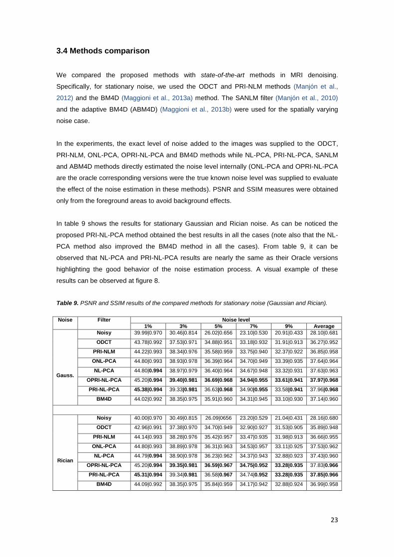
3.4 Methods comparison
We compared the proposed methods with state-of-the-art methods in MRI denoising.
Specifically, for stationary noise, we used the ODCT and PRI-NLM methods (Manjón et al.,
2012) and the BM4D (Maggioni et al., 2013a) method. The SANLM filter (Manjón et al., 2010)
and the adaptive BM4D (ABM4D) (Maggioni et al., 2013b) were used for the spatially varying
noise case.
In the experiments, the exact level of noise added to the images was supplied to the ODCT,
PRI-NLM, ONL-PCA, OPRI-NL-PCA and BM4D methods while NL-PCA, PRI-NL-PCA, SANLM
and ABM4D methods directly estimated the noise level internally (ONL-PCA and OPRI-NL-PCA
are the oracle corresponding versions were the true known noise level was supplied to evaluate
the effect of the noise estimation in these methods). PSNR and SSIM measures were obtained
only from the foreground areas to avoid background effects.
In table 9 shows the results for stationary Gaussian and Rician noise. As can be noticed the
proposed PRI-NL-PCA method obtained the best results in all the cases (note also that the NL-
PCA method also improved the BM4D method in all the cases). From table 9, it can be
observed that NL-PCA and PRI-NL-PCA results are nearly the same as their Oracle versions
highlighting the good behavior of the noise estimation process. A visual example of these
results can be observed at figure 8.
Table 9. PSNR and SSIM results of the compared methods for stationary noise (Gaussian and Rician).
Noise Filter Noise level
1% 3% 5% 7% 9% Average
Gauss.
Noisy 39.99|0.970 30.46|0.814 26.02|0.656 23.10|0.530 20.91|0.433 28.10|0.681
ODCT 43.78|0.992 37.53|0.971 34.88|0.951 33.18|0.932 31.91|0.913 36.27|0.952
PRI-NLM 44.22|0.993 38.34|0.976 35.58|0.959 33.75|0.940 32.37|0.922 36.85|0.958
ONL-PCA 44.80|0.993 38.93|0.978 36.39|0.964 34.70|0.949 33.39|0.935 37.64|0.964
NL-PCA 44.80|0.994 38.97|0.979 36.40|0.964 34.67|0.948 33.32|0.931 37.63|0.963
OPRI-NL-PCA 45.20|0.994 39.40|0.981 36.69|0.968 34.94|0.955 33.61|0.941 37.97|0.968
PRI-NL-PCA 45.38|0.994 39.33|0.981 36.63|0.968 34.90|0.955 33.58|0.941 37.96|0.968
BM4D 44.02|0.992 38.35|0.975 35.91|0.960 34.31|0.945 33.10|0.930 37.14|0.960
Rician
Noisy 40.00|0.970 30.49|0.815 26.09|0656 23.20|0.529 21.04|0.431 28.16|0.680
ODCT 42.96|0.991 37.38|0.970 34.70|0.949 32.90|0.927 31.53|0.905 35.89|0.948
PRI-NLM 44.14|0.993 38.28|0.976 35.42|0.957 33.47|0.935 31.98|0.913 36.66|0.955
ONL-PCA 44.80|0.993 38.89|0.978 36.31|0.963 34.53|0.957 33.11|0.925 37.53|0.962
NL-PCA 44.79|0.994 38.90|0.978 36.23|0.962 34.37|0.943 32.88|0.923 37.43|0.960
OPRI-NL-PCA 45.20|0.994 39.35|0.981 36.59|0.967 34.75|0.952 33.28|0.935 37.83|0.966
PRI-NL-PCA 45.31|0.994 39.34|0.981 36.58|0.967 34.74|0.952 33.28|0.935 37.85|0.966
BM4D 44.09|0.992 38.35|0.975 35.84|0.959 34.17|0.942 32.88|0.924 36.99|0.958

24
Figure 8. Example results of the compared filters for 9% of Rician noise. A Closed up is shown
to better appreciate the differences between compared methods (the method differences can be
better appreciated at sulcus areas).
In table 10 the results for spatially varying Gaussian and Rician noise are presented. The
proposed PRI-NL-PCA method obtained the best results in almost all the cases. Although
ABM4D method showed a good behavior for high levels of Gaussian noise it did not perform as
well for Rician noise (probably due to an inaccurate bias correction). A visual example of these
results can be observed at figure 9.
Table 10. PSNR and SSIM results of the compared methods for spatially varying noise.
Noise Filter Noise Level
1-3% 3-9% 5-15% 7-21% 9-27% Average
Gauss.
Noisy 34.34|0.900 24.80|0.621 20.36|0.442 17.44|0.328 15.26|0.253 22.44|0.508
ONL-PCA 41.60|0.987 35.94|0.959 33.23|0.928 31.41|0.897 30.07|0.867 34.45|0.928
NL-PCA 41.66|0.987 35.95|0.958 33.17|0.925 31.31|0.891 29.92|0.857 34.40|0.924
OPRI-NL-PCA 42.19|0.989 36.33|0.965 33.53|0.939 31.59|0.911 30.10|0.882 34.75|0.937
PRI-NL-PCA 42.25|0.989 36.30|0.965 33.52|0.939 36.61|0.911 30.16|0.883 34.77|0.937
ABM4D 40.45|0.980 35.48|0.960 33.10|0.930 31.48|0.900 30.24|0.870 34.15|0.928
SANLM 40.38|0.980 34.50|0.940 31.57|0.890 29.61|0.830 28.11|0.780 32.83|0.884
Rician
Noisy 34.35|0.900 24.87|0.621 20.50|0.441 17.64|0.325 15.50|0.247 22.57|0.507
ONL-PCA 41.59|0.987 35.87|0.958 32.99|0.925 30.93|0.890 29.28|0.854 34.13|0.923
NL-PCA 41.64|0.987 35.77|0.956 32.74|0.917 30.48|0.873 28.42|0.824 33.81|0.911
OPRI-NL-PCA 42.18|0.989 36.20|0.964 33.16|0.933 30.92|0.897 29.22|0.861 34.34|0.930
PRI-NL-PCA 42.23|0.989 36.19|0.964 33.15|0.934 30.87|0.897 28.83|0.856 34.25|0.928
ABM4D 40.43|0.980 34.41|0.940 31.27|0.890 28.80|0.820 26.55|0.740 32.29|0.874
SANLM 40.28|0.980 34.29|0.940 31.16|0.870 28.73|0.810 26.43|0.740 31.18|0.868

25
Figure 9. Example results of the compared filters for 9-27% of Rician noise. A Closed up is
shown to appreciate the differences between compared methods. Note that NL-PCA method
showed some artifacts for very high levels of noise due to non-cancelled components. Note
though that the PRI-NL-PCA method does not show any artifact due the different behavior of
the averaging process compared to the truncation PCA based process.
Finally, the processing times of the different compared methods were analyzed. The faster
method was the ODCT method with just 5 seconds on average followed by the PRI-NLM with
45 seconds. The SANLM took around 300 seconds. The proposed NL-PCA and PRI-NL-PCA
methods took 185 and 320 seconds respectively while the BM4D took 567 seconds when the
noise level was externally supplied to the method and 1900 seconds when it was internally
estimated from the data (we should note here that the increased processing time of ABM4D
may be caused by implementation issues since authors reported that ABM4D has only a slightly
higher processing time than BM4D).

26
Real data comparison
To compare the methods on real clinical data two datasets were used. The first was an MP-
RAGE T1w volumetric sequence from OASIS dataset acquired on a Siemens 1.5T Vision
scanner (Erlangen, Germany) with TR = 9.7 ms, TE = 4 ms, TI = 20 ms, TD = 200 ms, flip angle
= 10º, voxel resolution = 1x1x1.25 mm3 and 256x256x128 voxels.
We compared visually the proposed PRI-NL-PCA method with the BM4D method since the
noise in this volume is expected to be stationary. The stationary noise level in this case (2%)
was estimated using the Rician noise estimator proposed by Coupe et al (2010). BM4D method
used the estimated noise level provided by the Coupe´s method while the PRI-NL-PCA method
internally estimated the noise level as previously described. The filtering results for this first
dataset are shown in Figure 10. Both methods performed very well on this dataset (the BM4D
method seems to slightly over blur sulcal areas). The processing time for this dataset was 240
seconds for PRI-NL-PCA method while the BM4D method took 502 seconds.
The second dataset was obtained with a SENSE T1w volumetric sequence from Quirón
Hospital of Valencia (Spain) acquired on Philips Achieva 3 Tesla scanner (Netherlands) with
TR=9.5 ms, TE=4.6 ms and flip angle=8º, 256x256x120 voxels and voxel resolution of
0.96x0.96x1 mm3.
Figure 11 enables a visual comparison of the results produced using the PRI-NL-PCA and
ABM4D methods over this case with spatially varying noise. The PRI-NL-PCA method removed
the noise successfully while preserving fine details of the image, whereas the ABM4D method
slightly over smoothed some details. The processing time for this dataset was 227 seconds with
the PRI-NL-PCA method and 398 seconds with the ABM4D filter. The reduced processing time
of ABM4D method compared to the results obtained with the brainweb phantom may be
explained by the fact that background of this volume is set to zero by the scanner due to the use
of the SENSE sequence and probably the ABM4D method skipped the calculations at this area
thus reducing significantly the processing time.

27
Figure 10. Example of denoising results (stationary noise). From left to right: Original noisy
image, PRI-NL-PCA result and BM4D result. Although both methods performed very well the
BM4D slightly over blurred the image (this can be noticed in the sulcus areas at the close up).

28
Figure 11. Example of denoising results (spatially varying noise). From left to right: Original
noisy image, PRI-NL-PCA result and ABM4D result. Although both methods performed very
well, the ABM4D slightly over blurred the image (this can be clearly noticed in the cerebellar
area).

29
4. Discussion
In this paper we have proposed a novel PCA based filter that takes benefit from sparseness
properties of groups of similar patches to reduce the noise effectively while minimally affecting
the underlying signal. We have also shown that using this filter to create a guide image for the
rotationally invariant non-local means filter enables to obtain the best denoising results in the
comparison.
The proposed methods have been compared with state-of-the-art methods for both stationary
and spatially varying noise conditions with Gaussian and Rician noises and obtained the best
results. The improved performance of the proposed methods compared to previously proposed
methods can be explained by the use of self-similarity and sparseness properties of the images.
In fact, grouping similar patches to create a homogenous group allows obtaining a very sparse
representation through the use of PCA decomposition. In this sense, our patch selection was
improved by performing the patch grouping over a pre-filtered image to make it more robust on
very noisy conditions. Besides, differently from other PCA based methods, the use of the pre-
filtered guide image obtained with the NL-PCA method enables to accurately estimate the voxel
similarities in a rotationally invariant manner that naturally results in a very effective noise
reduction within the non-local means strategy.
One of the most significant contributions of this paper is the noise estimation technique within
NL-PCA method. Local noise estimation is performed in a local manner from the eigenvalues
distribution of the local PCA decomposition with allows to estimate and filter spatially varying
noise fields. Furthermore, a novel Rician bias correction technique has been introduced that
improves original signal estimation. This technique not only enables the estimation of the local
noise level but also enables to automatically estimate the number of significant components to
be retained in a fully automatic manner. It’s worth noting that this technique can be applied to
many other problems where the number of components has to be estimated (for example for
dimensionality reduction assuming a random behavior of the non-significant variability sources).
We have also presented a novel method for correcting the Rician noise underestimation.
Despite the simplicity of this method it has been experimentally demonstrated its ability to obtain
very fast and accurate local noise estimations improving a previous existing method.
From an efficacy point of view, the proposed PRI-NL-PCA method has been shown to be almost
two times faster than BM4D method and six times faster than the ABM4D method. The
proposed PRI-NL-PCA method obtained an average improvement of almost 1 dB compared to
the state-of-the-art BM4D method for stationary Rician noise. From a practical point of view, the
proposed method can be applied to both stationary of spatially varying noise cases in a fully
automatic manner that makes it ideal for a use within a preprocessing pipeline for automated
MRI analysis tasks.
30
It should be noted though that the proposed methods in this paper assume the presence of
white noise in the images. This condition may not be satisfied when using acceleration
techniques such as partial Fourier or compressed sensing. In these cases, the methods
proposed in this paper cannot be directly applied due to the correlated nature of the noise. This
situation will be studied in future works.
Acknowledgments
We are grateful to Dr. Matteo Mangioni and Dr. Alessandro Foi for their help on running their
BM4D method in our comparisons. We want also to thank Dr. Luis Martí-Bonmatí and Dr. Angel
Alberic from Quirón Hospital of Valencia for providing the real clinical data used in this paper.
This study has been carried out with financial support from the French State, managed by the
French National Research Agency (ANR) in the frame of the Investments for the future
Programme IdEx Bordeaux (ANR-10-IDEX-03-02), Cluster of excellence CPU and TRAIL (HR-
DTI ANR-10-LABX-57).

31
References
Aharon M, Elad M, Bruckstein A M. 2006. K-SVD: an algorithm for designing over complete
dictionaries for sparse representation. IEEE Trans. Signal Process., 54:4311–4322.
Aja-Fernandez, S., Tristan, A., Alberola-Lopez, C., 2009. Noise estimation in single and multiple
coil magnetic resonance data based on statistical models. Magn Reson Imaging 27, 1397-1409.
Bao L, Liu W, Zhu Y, Pu Z, Magnin I. 2008. Sparse Representation Based MRI Denoising with
Total Variation. ICSP2008 Proceedings
Bao L, Robini M, Liu W, Zhu Y. 2013. Structure-adaptive sparse denoising for diffusion-tensor
MRI. Medical Image Analysis, 17(4), 442–457.
Bydder M, Du J (2003) Noise reduction in multiple-echo data sets using singular value
decomposition. Magn Reson Imaging 24(7): 849–856.
Buades A, Coll B and Morel J.M. 2005. A non-local algorithm for image denoising. IEEE Int.
Conf. on Computer Vision and Pattern Recognition (CPVR) 2, 60–65.
Collins D.L., Zijdenbos A.P., Kollokian V., Sled J.G., Kabani N.J., Holmes C.J. and Evans A.C.
1998. Design and construction of a realistic digital brain phantom. IEEE Trans. Med. Imaging,
17, 463–468.
Coupé P., Yger P., Prima S., Hellier P., Kervrann C. and Barillot C. 2008. An optimized
blockwise nonlocal means denoising filter for 3-D magnetic resonance images. IEEE Trans.
Med. Imaging, 27, 425–441.
Coupé P., Manjón J.V., Gedamu E., Arnold D., Robles M. and Collins D.L. 2010. Robust Rician
noise estimation for MR images. Med. Image Anal, 14, 483–493.
Coupé P, Munz M, Manjón J. V., Ruthazer E., Collins D. L. 2012. A CANDLE for a deeper in
vivo insight. Medical Image Analysis, 16 (4):849-864.
Deledalle C, Salmon J, Dalalyan A. 2011. Image denoising with patch based PCA: local versus
global. BMVC 2011

32
Elad M and Aharon M. 2006. Image Denoising Via Sparse and Redundant representations over
Learned Dictionaries, the IEEE Trans. on Image Processing, 15(12), pp. 3736-3745.
Fan Lam S, Babacan D, Haldar JP, Weiner MW, Schuff N, et al. 2013. Denoising diffusion-
weighted magnitude MR images using rank and edge constraints. Magnetic Resonance in
Medicine, 69(6): 1–13.
Guleryuz, O.G., 2003. Weighted overcomplete denoising. In: Proceedings of the Asilomar
Conference on Signals and Systems.
He, L., Greenshields, I.R., 2009. A nonlocal maximum likelihood estimation method for Rician
noise reduction in MR images. IEEE Trans Med Imaging 28, 165-172.
Katkovnik V, Foi A, Egiazarian K, and Astola J. 2010. From local kernel to nonlocal multiple-model image denoising. Int. J. Computer Vision, 86(1): 1-32
Kim DW, Kim C, Kim DH, Lim, DH. 2011. Rician nonlocal means denoising for MR images using
nonparametric principal component analysis. EURASIP Journal on Image and video
Processing, 2011:15.
Koay CG and Basser PJ. 2006. Analytically exact correction scheme for signal extraction from
noisy magnitude MR signals. Journal of Magnetic Resonance; 179: 477-482.
Kwan R.K.-S., Evans A.C. and Pike G.B. 1999. MRI simulation-based evaluation of image-
processing and classification methods. IEEE Trans. Med. Imaging, 18, 1085–1097.
Mairal J, Elad M, Sapiro G. 2008. Sparse learned representations for image restoration.
IASC2008:, Yokohama, Japan
Maggioni M., Katkovnik V., Egiazarian K, Foi A. 2013. A Nonlocal Transform-Domain Filter for
Volumetric Data Denoising and Reconstruction., IEEE Trans. Image Process., 22(1),pp. 119-
133.
Maggioni M, Foi A. 2012. Nonlocal Transform-Domain Denoising of Volumetric Data With
Groupwise Adaptive Variance Estimation. Proc. SPIE Electronic Imaging (EI), 2012, San
Francisco, CA, USA.

33
Manjón J.V., Carbonell-Caballero J., Lull J.J., Garcia-Martí G., Martí-Bonmatí L. and Robles M.
2008. MRI denoising using non-local means. Med. Image Anal, 4 , 514–523.
Manjón J.V., Thacker N.A., Lull J.J., Garcia-Martí G., Martí-Bonmatí L., Robles M. 2009.
Multicomponent MR Image Denoising. International Journal of Biomedical imaging. Article ID
756897.
Manjón J.V., Coupé P., Martí-Bonmatí L., Robles M. and Collins D.L. 2010. Adaptive non-local
means denoising of MR images with spatially varying noise levels. J. Magn. Reson. Imaging,
31, 192–203.
Manjón J. V., Coupé P., Buades A., Collins D. L., Robles M. 2012. New Methods for MRI
Denoising based on Sparseness and Self-Similarity. Medical Image Analysis, 16(1): 18-27.
Manjón J.V., Coupé P., Concha L., Buades A., Collins D. L., Robles M. 2013. Diffusion
Weighted Image Denoising using overcomplete Local PCA. PLoS ONE 8(9): e73021.
doi:10.1371/journal.pone.0073021.
Mohan J, Krishnaveni V, Guo Y. 2014. A survey on the magnetic resonance image denoising
methods. Biomedical Signal Processing and Control, 9, 56–69
Muresan D.D. and Parks T.W. 2003. Adaptive principal components and image denoising. IEEE
Int. Conf. Image Process., 1, 101–104.
Nowak R. 1999. Wavelet-based Rician noise removal for magnetic resonance imaging. IEEE
Trans. Image Process, 8, 1408–1419.
Pan X, Zhang X and Lyu S. 2012. Blind Local Noise Estimation for Medical Images Reconstructed from Rapid Acquisition, SPIE 2012. San Diego, CA.
Protter M. and Elad M. 2009. Image Sequence Denoising Via Sparse and Redundant
Representations. IEEE Trans. on Image Processing, Vol. 18(1), Pages 27-36.
Pyatykh S., Hesser J, and Zheng L. 2013. Image Noise Level Estimation by Principal
Component Analysis, IEEE TIP,22, 687-699.

34
Rajan J, Veraart J, Audekerke J, Verhoye M, Sijbers J. 2012. "Nonlocal maximum likelihood
estimation method for denoising multiple-coil magnetic resonance images", Magn Reson
Imaging, 30,1512-1518.
Rajan J, Den Dekker A, Sijbers J. 2014. A new non local maximum likelihood estimation method
for Rician noise reduction in Magnetic Resonance images using the Kolmogorov-Smirnov test.
Signal Processing, 103,16-23.
Salmon J, Willett R, Arias-Castro E. 2012. A two-stage denoising filter: the preprocessed
Yaroslavsky filter. Statistical Signal Processing Workshop (SSP), 2012 IEEE, 464-467.
Sijbers J., Poot D. H. J., den Dekker A. J., and Pintjens W. 2007. Automatic estimation of the
noise variance from the histogram of a magnetic resonance image. Physics in Medicine and
Biology, vol. 52(5), pp. 1335-1348.
Tristán-Vega A, García-Pérez V, Aja-Fernández S. 2012. Efficient and Robust Nonlocal Means
Denoising of MR Data Based on Salient Features Matching, Computer Methods and Programs
in Biomedicine. 105(2):131–144.
Van De Ville D. and Kocher M. 2010. Non-Local Means with Dimensionality Reduction and SURE-Based Parameter Selection, IEEE TIP, 20(9), 2683-2690.
Vishal Patel, Yonggang Shi, Paul M. Thompson, Arthur W. Toga. 2011. K-SVD FOR HARDI
DENOISING. IEEE International Symposium on Biomedical Imaging: From Nano to Macro.
Wang Z., Bovik A.C., Sheikh H.R. and Simoncelli E.P. 2004. Image quality assessment: from
error visibility to structural similarity. IEEE Trans. Image Process., 13, 600–612.
Wiest-Daesslé N., Prima S., Coupé P., Morrissey S.P. and Barillot C. 2008. Rician noise
removal by non-local means filtering for low signal-to-noise ratio MRI: applications to DR-MRI.
MICCAI, 11, 171–179.
Yaroslavsky, L.P., Egiazarian, K., Astola, J., 2000. Transform domain image restoration
methods: review, comparison and interpretation. TICSP Series #9, TUT, ISBN 952-15-0471-4.
Zhang L, Dong W, Zhanga D, Shib G. 2010. Two-stage image denoising by principal component analysis with local pixel grouping. Pattern Recognition, 43(4),1531-1549. Zhang, YQ ; Ding, Y ; Liu, JY ; Guo, ZM. 2013. Guided image filtering using signal subspace projection. IET Image Processing, 7(3), 270-279.

35
Zhang, YQ ; Liu, JY ; Li, MD ; Guo, ZM. 2014. Joint image denoising using adaptive principal component analysis and self-similarity, Information Sciences, 259,128-141.