moving average method maths ppt
TRANSCRIPT
By:-HEEMA
SUMANT
& ABHISHEK
Moving average method
A quantitative method of forecasting or smoothing a time series by averaging each successive group (no. of observations) of data values.
term MOVING is used because it is obtained by summing and averaging the values from a given no of periods, each time deleting the oldest value and adding a new value.
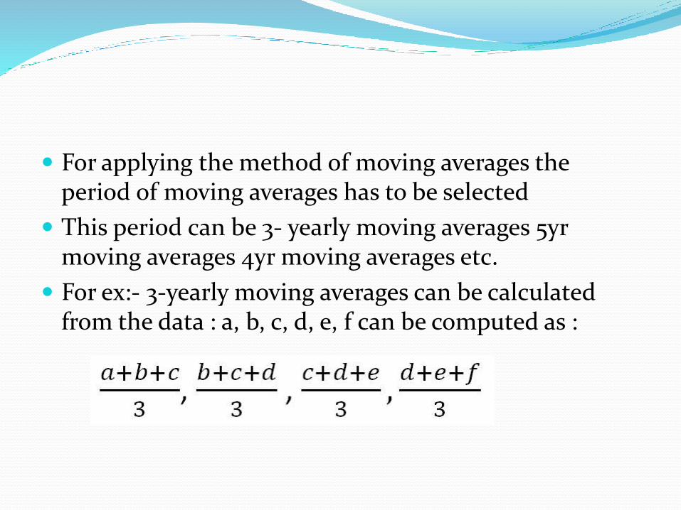
For applying the method of moving averages the period of moving averages has to be selected
This period can be 3- yearly moving averages 5yr moving averages 4yr moving averages etc.
For ex:- 3-yearly moving averages can be calculated from the data : a, b, c, d, e, f can be computed as :
If the moving average is an odd no of values e.g., 3 years, there is no problem of centring it. Because the moving total for 3 years average will be centred besides the 2nd year and for 5 years average be centred besides 3rd year.
But if the moving average is an even no, e.g., 4 years moving average, then the average of 1st 4 figures will be placed between 2nd and 3rd year.
This process is called centering of the averages. In case of even period of moving averages, the trend values are obtained after centering the averages a second time.
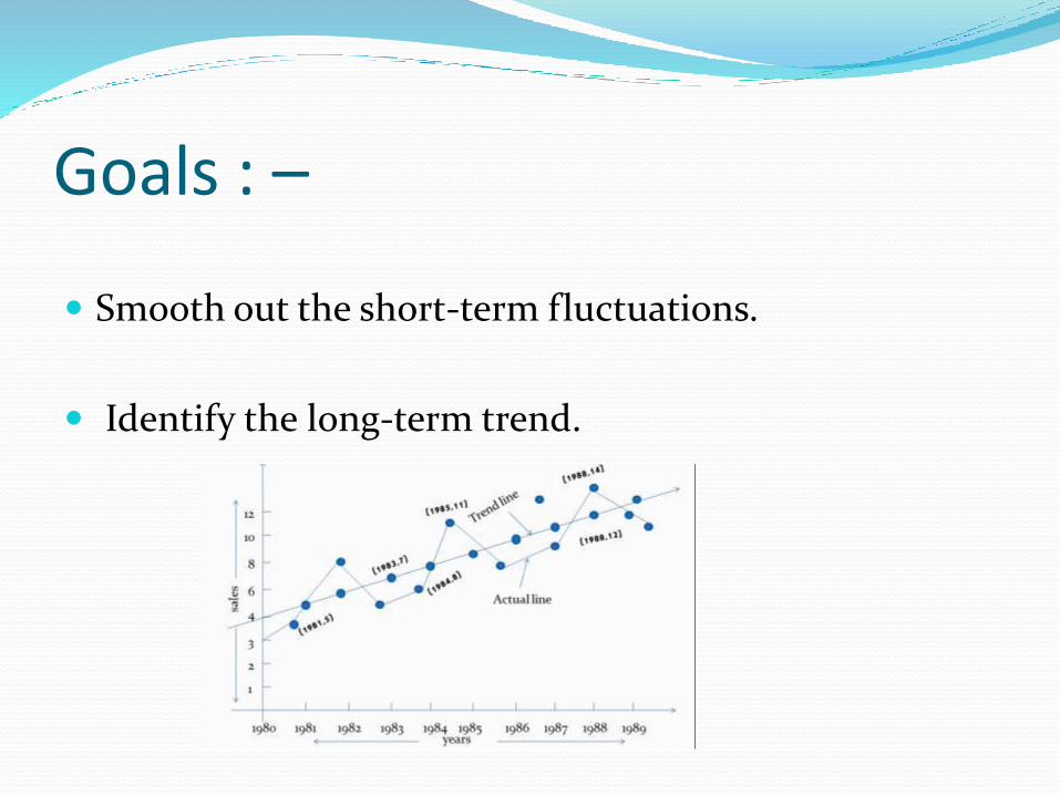
Goals : –
Smooth out the short-term fluctuations.
Identify the long-term trend.
MERITS Of Moving average method
simple method.
flexible method.
OBJECTIVE :-
If the period of moving averages coincides with the period of cyclic fluctuations in the data , such fluctuations are automatically eliminated
This method is used for determining seasonal, cyclic and irregular variations beside the trend values.
LIMITATIONS Of Moving average method
No trend values for some year.
M.A is not represented by mathematical function - not helpful in forecasting and predicting.
The selection of the period of moving average is a difficult task.
In case of non-linear trend the values obtained by this method are biased in one or the other direction.
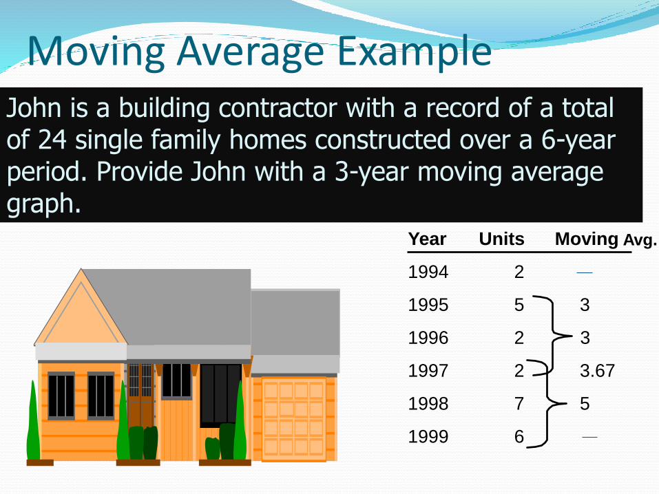
Moving Average Example
Year Units Moving
1994 2
1995 5 3
1996 2 3
1997 2 3.67
1998 7 5
1999 6
John is a building contractor with a record of a total of 24 single family homes constructed over a 6-year period. Provide John with a 3-year moving average graph.
Avg.
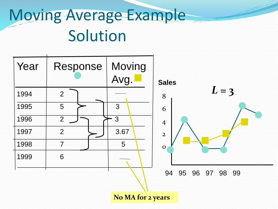
Moving Average Example Solution
Year Response Moving
Avg.
1994 2
1995 5 3
1996 2 3
1997 2 3.67
1998 7 5
1999 6
94 95 96 97 98 99
8
6
4
2
0
Sales
L = 3
No MA for 2 years
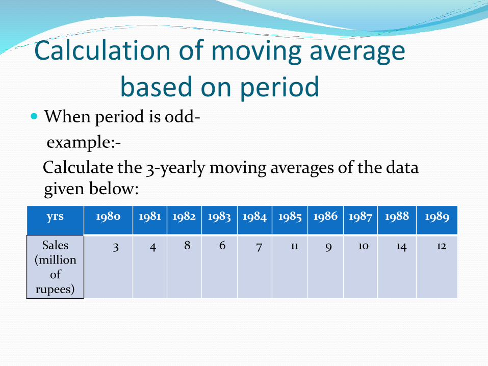
Calculation of moving average based on period
When period is odd-
example:-
Calculate the 3-yearly moving averages of the data given below:
yrs 1980 1981 1982 1983 1984 1985 1986 1987 1988 1989
Sales (million
of rupees)
3 4 8 6 7 11 9 10 14 12
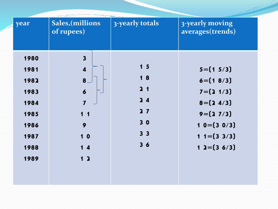
year Sales,(millions of rupees)
3-yearly totals 3-yearly moving averages(trends)
1980198119821983198419851986198719881989
348671 191 01 41 2
1 51 82 12 42 73 03 33 6
5=(1 5/3)6=(1 8/3)7=(2 1/3)8=(2 4/3)9=(2 7/3)1 0=(3 0/3)1 1=(3 3/3)1 2=(3 6/3)
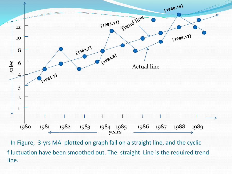
In Figure, 3-yrs MA plotted on graph fall on a straight line, and the cyclic
f luctuation have been smoothed out. The straight Line is the required trend line.
1980 1981 1982 1983 1984 1985 1986 1987 1988 1989
1
2
3
years
sale
s
4
6
8
10
12
Actual line
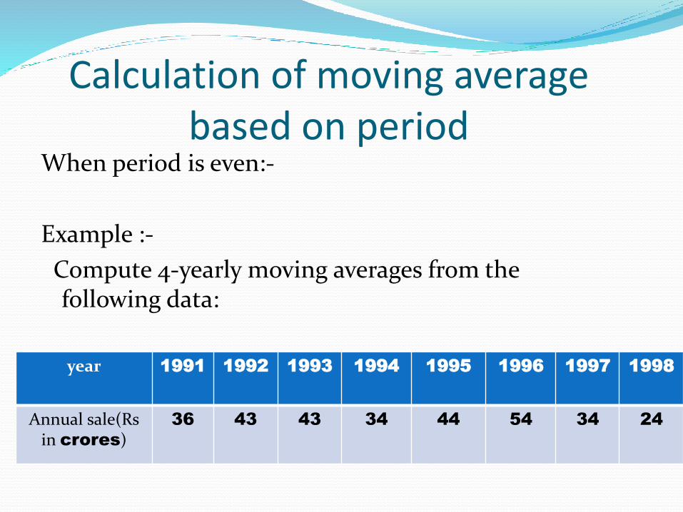
Calculation of moving average based on period
When period is even:-
Example :-
Compute 4-yearly moving averages from the following data:
year 1991 1992 1993 1994 1995 1996 1997 1998
Annual sale(Rsin crores)
36 43 43 34 44 54 34 24
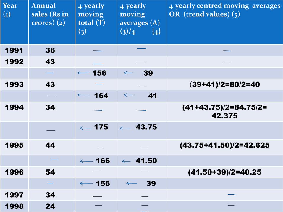
Year (1)
Annual sales (Rs in crores) (2)
4-yearly moving total (T) (3)
4-yearly moving averages (A) (3)/4 {4}
4-yearly centred moving averages OR (trend values) (5)
1991 36
1992 43
156 39
1993 43 (39+41)/2=80/2=40
164 41
1994 34 (41+43.75)/2=84.75/2=
42.375
175 43.75
1995 44 (43.75+41.50)/2=42.625
166 41.50
1996 54 (41.50+39)/2=40.25
156 39
1997 34
1998 24
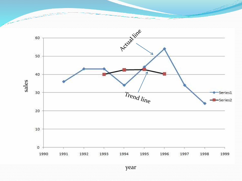
sale
s
year
Method of least squares This is the best method for obtaining trend values.
It provides a convenient basis for obtaining the line of best fit in a series.
Line of the best fit is a line from which the sum of the deviations of various points on its either side is zero.
The sum of the squares of the deviation of various points from the line of best fit is the least. – That is why this method is known as method of least squares.
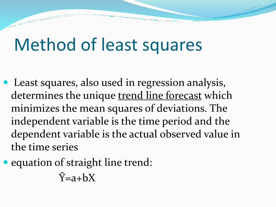
Method of least squares
Least squares, also used in regression analysis, determines the unique trend line forecast which minimizes the mean squares of deviations. The independent variable is the time period and the dependent variable is the actual observed value in the time series
equation of straight line trend:
Y=a+bX
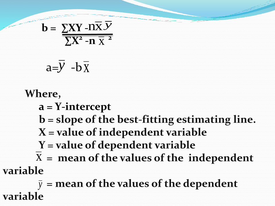
b = ∑XY -∑X2 -n 2
a= -b
Where,a = Y-interceptb = slope of the best-fitting estimating line.X = value of independent variableY = value of dependent variable
= mean of the values of the independent variable
= mean of the values of the dependent variable
x
x
y
xn
y x
y
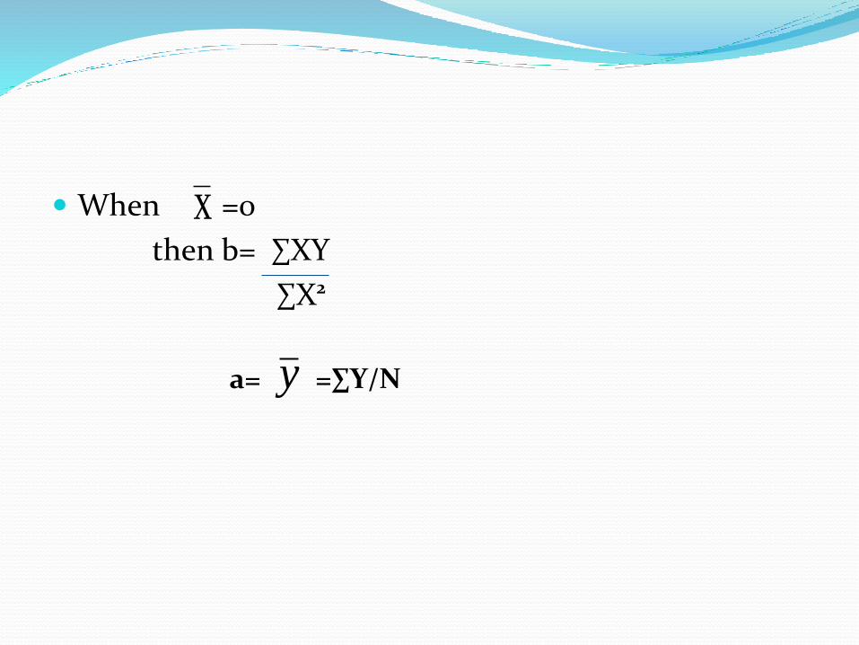
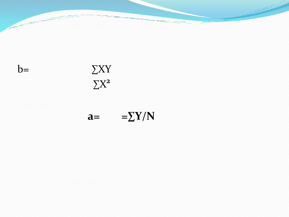
When =0
then b= ∑XY
∑X2
a= =∑Y/N
x
y
MERITS This method gives the trend values for the entire time
period.
This method can be used to forecast future trend because trend line establishes a functional relationship between the values and the time.
This is a completely objective method.
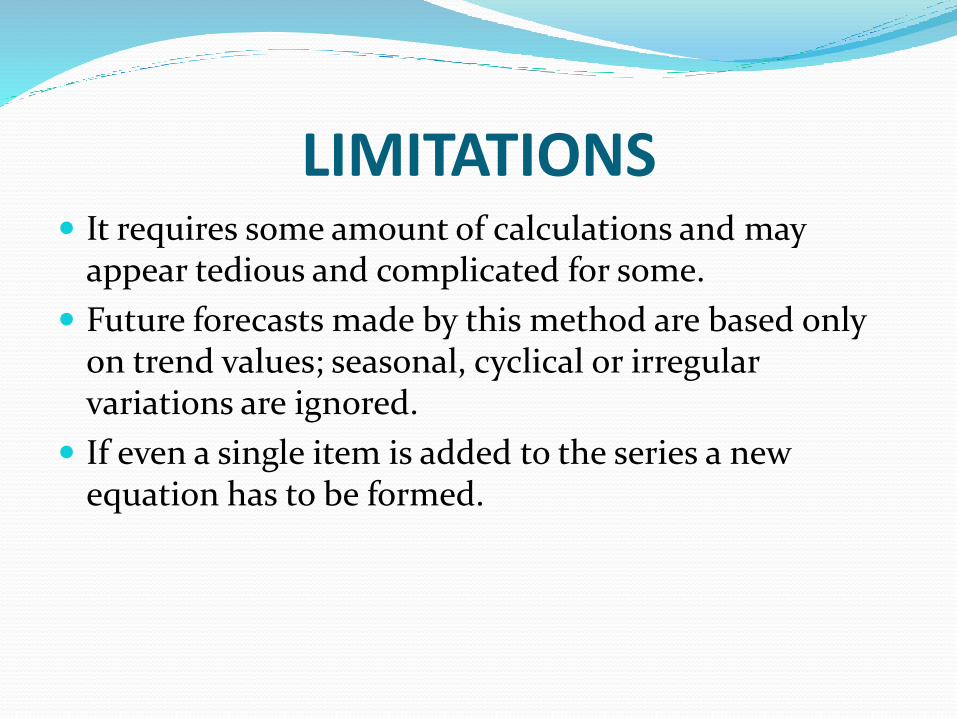
LIMITATIONS It requires some amount of calculations and may
appear tedious and complicated for some.
Future forecasts made by this method are based only on trend values; seasonal, cyclical or irregular variations are ignored.
If even a single item is added to the series a new equation has to be formed.
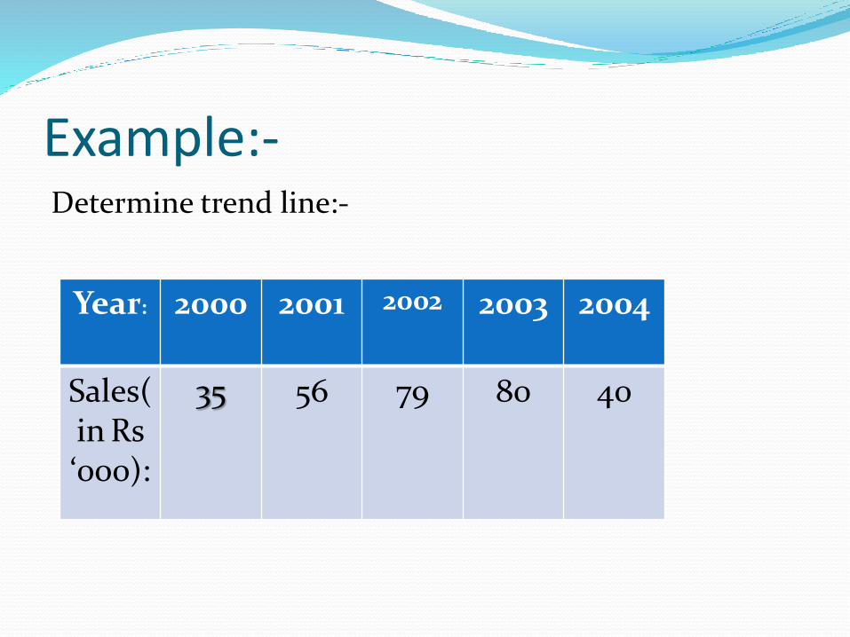
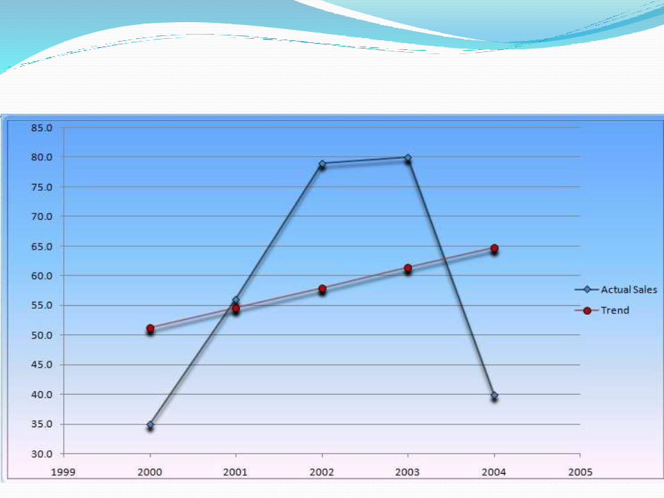
Example:-Determine trend line:-
Year: 2000 2001 2002 2003 2004
Sales(in Rs‘000):
35 56 79 80 40
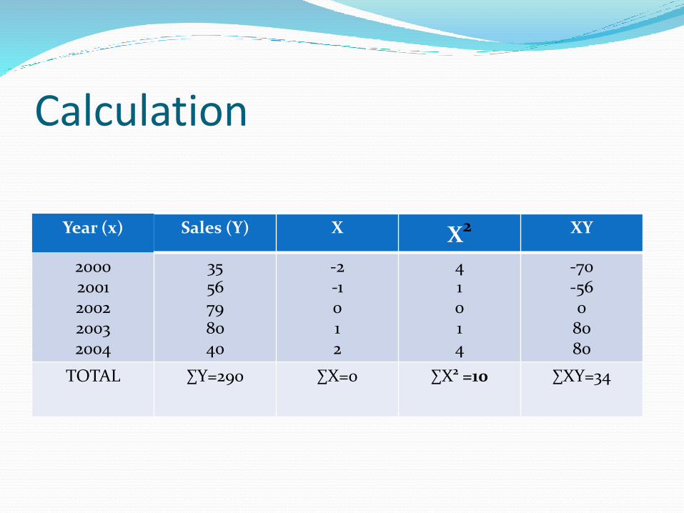
Calculation
Year (x) Sales (Y) X X2 XY
20002001200220032004
3556798040
-2-1012
41014
-70-560
8080
TOTAL ∑Y=290 ∑X=0 ∑X2 =10 ∑XY=34
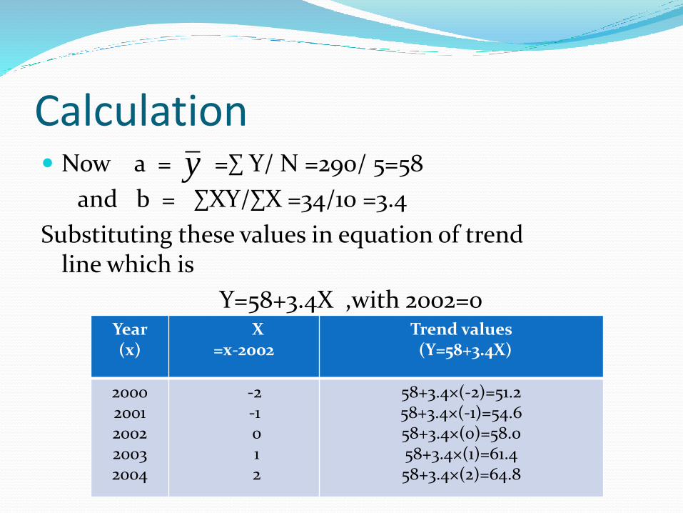
Calculation Now a = =∑ Y/ N =290/ 5=58
and b = ∑XY/∑X =34/10 =3.4
Substituting these values in equation of trend line which is
Y=58+3.4X ,with 2002=0
y
Year (x)
X=x-2002
Trend values (Y=58+3.4X)
20002001200220032004
-2-1012
58+3.4×(-2)=51.258+3.4×(-1)=54.658+3.4×(0)=58.058+3.4×(1)=61.458+3.4×(2)=64.8
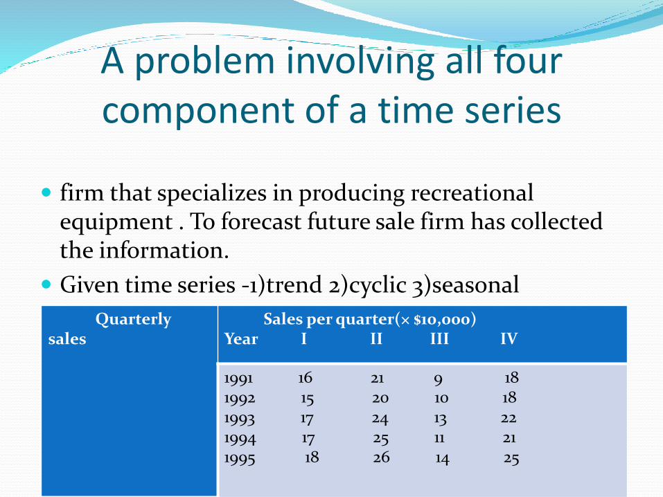
A problem involving all four component of a time series
firm that specializes in producing recreational equipment . To forecast future sale firm has collected the information.
Given time series -1)trend 2)cyclic 3)seasonal
Quarterly sales
Sales per quarter(× $10,000)Year I II III IV
1991 16 21 9 181992 15 20 10 181993 17 24 13 221994 17 25 11 211995 18 26 14 25
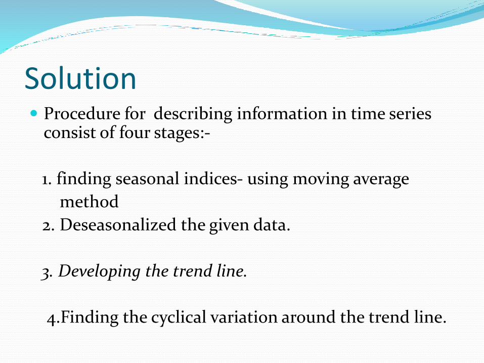
Solution Procedure for describing information in time series
consist of four stages:-
1. finding seasonal indices- using moving average
method
2. Deseasonalized the given data.
3. Developing the trend line.
4.Finding the cyclical variation around the trend line.
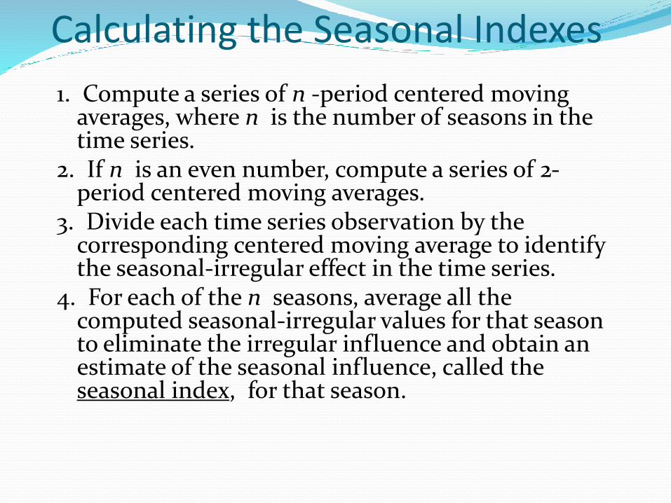
Calculating the Seasonal Indexes
1. Compute a series of n -period centered moving averages, where n is the number of seasons in the time series.
2. If n is an even number, compute a series of 2-period centered moving averages.
3. Divide each time series observation by the corresponding centered moving average to identify the seasonal-irregular effect in the time series.
4. For each of the n seasons, average all the computed seasonal-irregular values for that season to eliminate the irregular influence and obtain an estimate of the seasonal influence, called the seasonal index, for that season.
Deseasonalizing the Time Series
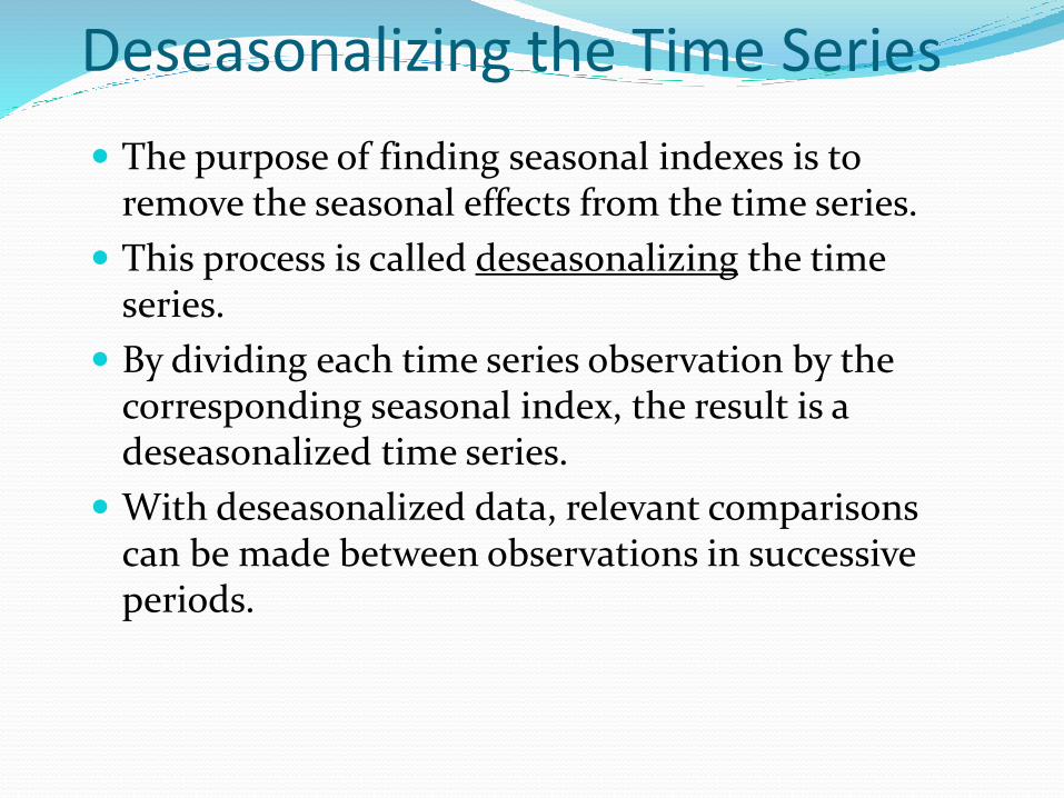
The purpose of finding seasonal indexes is to remove the seasonal effects from the time series.
This process is called deseasonalizing the time series.
By dividing each time series observation by the corresponding seasonal index, the result is a deseasonalized time series.
With deseasonalized data, relevant comparisons can be made between observations in successive periods.
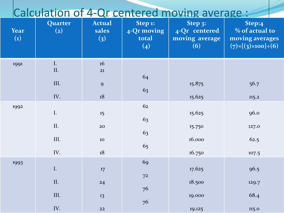
Calculation of 4-Qr centered moving average :
Year (1)
Quarter (2)
Actual sales
(3)
Step 1: 4-Qr moving
total (4)
Step 3: 4-Qr centered
moving average (6)
Step:4 % of actual to
moving averages (7)={(3)×100}÷(6)
1991 I.II.
III.
IV.
1621
9
18
64
6315.875
15.625
56.7
115.2
1992I.
II.
III.
IV.
15
20
10
18
62
63
63
65
15.625
15.750
16.000
16.750
96.0
127.0
62.5
107.5
1993I.
II.
III.
IV.
17
24
13
22
69
72
76
76
17.625
18.500
19.000
19.125
96.5
129.7
68.4
115.0
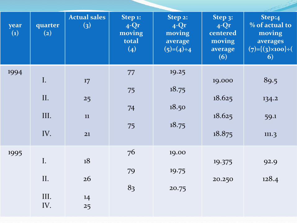
year (1)
quarter (2)
Actual sales (3)
Step 1: 4-Qr
moving total
(4)
Step 2: 4-Qr
moving average
(5)=(4)÷4
Step 3: 4-Qr
centered moving average
(6)
Step:4 % of actual to
moving averages
(7)={(3)×100}÷(6)
1994I.
II.
III.
IV.
17
25
11
21
77
75
74
75
19.25
18.75
18.50
18.75
19.000
18.625
18.625
18.875
89.5
134.2
59.1
111.3
1995I.
II.
III.IV.
18
26
1425
76
79
83
19.00
19.75
20.75
19.375
20.250
92.9
128.4
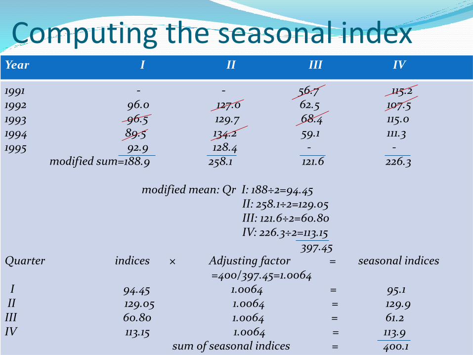
Computing the seasonal indexYear I II III IV
1991 - - 56.7 115.21992 96.0 127.0 62.5 107.51993 96.5 129.7 68.4 115.0 1994 89.5 134.2 59.1 111.31995 92.9 128.4 - -
modified sum=188.9 258.1 121.6 226.3
modified mean: Qr I: 188÷2=94.45 II: 258.1÷2=129.05III: 121.6÷2=60.80IV: 226.3÷2=113.15
397.45Quarter indices × Adjusting factor = seasonal indices
=400/397.45=1.0064I 94.45 1.0064 = 95.1
II 129.05 1.0064 = 129.9III 60.80 1.0064 = 61.2IV 113.15 1.0064 = 113.9
sum of seasonal indices = 400.1

Calculation 0f deaseasonalised time series values
Year(1)
Quarter (2)
Actual sales (3)
Seasonal index/100(4)
Deseasonalized sales (5)=(3)÷(4)
1991 IIIIIIIV
1621918
0.9511.2990.6121.139
16.816.214.715.8
1992 IIIIIIIV
15201018
0.9511.2990.6121.139
15.815.416.315.8
1993 IIIIIIIV
17241322
0.9511.2990.6121.139
17.918.521.219.3
1994 IIIIIIIV
17251121
0.9511.2990.6121.139
17.919.218.018.4
1995 IIIIIIIV
18261425
0.9511.2990.6121.139
18.920.022.921.9
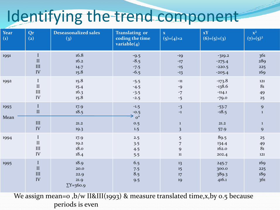
Identifying the trend componentYear (1)
Qr (2)
Deseasonalized sales(3)
Translating or coding the time variable(4)
x(5)=(4)×2
xY (6)=(5)×(3)
x² (7)=(5)²
1991 IIIIIIIV
16.816.214.715.8
-9.5-8.5-7.5-6.5
-19-17-15-13
-319.2-275.4-220.5-205.4
361289225169
1992 IIIIIIIV
15.815.416.315.8
-5.5-4.5-3.5-2.5
-11-9-7-5
-173.8-138.6-114.1-79.0
121814925
1993
Mean
III
IIIIV
17.918.5
21.219.3
-1.5-0.5
0*0.51.5
-3-1
13
-53.7-18.5
21.257.9
91
19
1994 IIIIIIIV
17.919.218.018.4
2.53.54.55.5
57911
89.5134.4162.0202.4
254981121
1995 IIIIIIIV
18.920.022.921.9
∑Y=360.9
6.57.58.59.5
13151719
245.7300.0389.3416.1
169225189361
We assign mean=0 ,b/w II&III(1993) & measure translated time,x,by 0.5 becauseperiods is even
b= ∑XY
∑X2
a= =∑Y/N
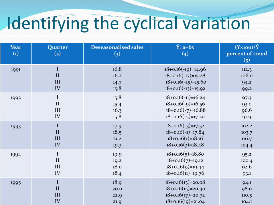
Identifying the cyclical variationYear (1)
Quarter (2)
Deseasonalised sales (3)
Y=a+bx(4)
(Y×100)/Y percent of trend
(5)
1991 IIIIIIIV
16.816.214.715.8
18+0.16(-19)=14.96 18+0.16(-17)=15.2818+0.16(-15)=15.60 18+0.16(-13)=15.92
112.3106.094.299.2
1992 IIIIIIIV
15.815.416.315.8
18+0.16(-11)=16.24 18+0.16(-9)=16.5618+0.16(-7)=16.88 18+0.16(-5)=17.20
97.393.096.691.9
1993 IIIIIIIV
17.918.521.219.3
18+0.16(-3)=17.52 18+0.16(-1)=17.84 18+0.16(1)=18.16 18+0.16(3)=18.48
102.2103.7116.7104.4
1994 IIIIIIIV
19.919.218.018.4
18+0.16(5)=18.80 18+0.16(7)=19.12 18+0.16(9)=19.44 18+0.16(11)=19.76
95.2100.492.693.1
1995 IIIIIIIV
18.920.022.921.9
18+0.16(13)=20.0818+0.16(15)=20.4018+0.16(17)=20.7218+0.16(19)=21.04
94.198.0110.5104.1
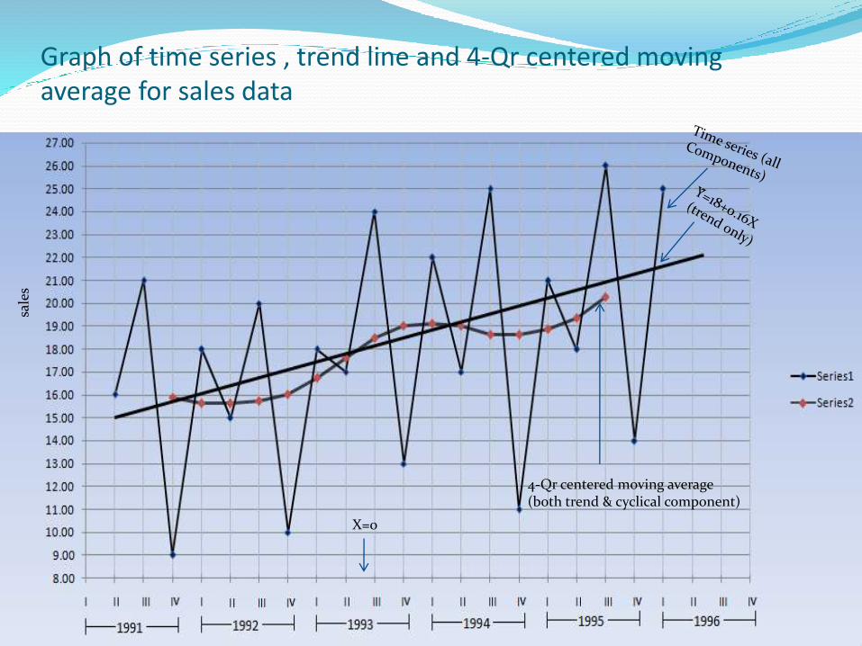
Graph of time series , trend line and 4-Qr centered moving average for sales data
4-Qr centered moving average(both trend & cyclical component)
sale
s
X=0