morphological in uences on the recognition of monosyllabic
TRANSCRIPT
Morphological influences on the recognition of monosyllabic monomorphemic words
R. H. Baayen
Radboud University Nijmegen and Max Planck Institute for Psycholinguistics, P.O. Box 310, 6500 AH,
Nijmegen, The Netherlands
e-mail: [email protected]
L. B. Feldman
State University of New York at Albany, Department of Psychology, SS112, Albany, New York 12222 USA
e-mail: [email protected]
R. Schreuder
Radboud University Nijmegen, P.O. Box 310, 6500 AH, Nijmegen, The Netherlands
e-mail: [email protected]
1
Introduction
Balota, Cortese, Sergent-Marschall, Spieler, and Yap (2004) have cautioned researchers in the field about
the drawbacks of factorial designs where variables are manipulated in a noncontinuous manner and effects
are assessed in terms of the presence or absence of a significant effect. They have eloquently demonstrated
for us the power of regression analyses based on hundreds or even thousands of data points and the potential
to consider simultaneously, as predictors, many properties of words that historically have been factorially
manipulated in separate experiments. Moreover, they have demonstrated that because regression analyses
give us the potential to examine the proportion of variance that a set of variables can account for, they permit
us to make comparisons across experimental tasks (e.g., lexical decision and naming) or across subject groups
(e.g., older and younger readers).
According to Balota et al., “The search for a significant effect does not typically motivate researchers
to report the amount of variance that a given factor accounts for in a design. The latter information may
ultimately be more important than the effects that reach the magical level of significance” (p. 285). From
their regression analyses, multiple insights based on a new type of evidence emerge. One insight is that
the naming task is relatively more influenced by form variables and that the lexical decision task is more
influenced by semantic variables. A second is that frequency plays a more substantial role in the lexical
decision task than in the naming task.
In their rich and influential paper, Balota and colleagues have tackled longstanding controversies about
the role of neighborhood density and have compared several of the well-published measures of frequency
(Kucera & Francis, 1967; celex, Baayen, Piepenbrock & Gulikers; Zeno, Ivens, Millard, & Duvvuri, 1995;
hal (1997); MetaMetrics, 2003) with respect to their linear (and quadratic) contributions to performance in
the lexical decision and naming tasks. They determined that the Zeno frequency norms (Zeno et al., 1995)
had a ”consistently large influence across groups and tasks.” Therefore, in subsequent multiple regression
analyses, justified by the percentage of variance it accounted for, they focused on the (linear) contributions of
Zeno frequency norms as well as the contribution of subjective frequency (Balota, Pilotti, & Cortese, 2001)
to performance in visual lexical decision and word naming.
2
In the primary regression analyses based on a large-scale data set, they made use of a hierarchical
regression analysis where they treated their expansive collection of variables in three steps. In step 1, they
included a set of indicator variables for the phonetic features of the word’s initial segment, in order to capture
variation caused by the differences in sensitivity of the voice key to the acoustic properties of the speech
signal. Lexical predictors including word length, neighborhood size, various consistency measures as well as
subjective frequency (Balota et al., 2001) and objective frequency based on Zeno et al. (1995) were entered
into the model at step 2. Then, in step 3, they brought semantic variables into the regression analyses,
dividing them into three blocks. The first block included Nelson set size (Nelson, McEvoy, & Schreiber,
1998), and imageability based on Toglia and Battig (1978). The second block included imageability based
on Cortese and Fugett (2003) and the third block included semantic connectivity measures from Steyvers
and Tanenbaum (2004).
The study of Balota et al. represents a rigorous analysis that is consistent with twenty years of research
on word recognition. Nevertheless, Balota et al. also raised a number of methodological issues inviting
further research and clarification. A first such issue is potential non-linearities in the relation between
predictors and response latencies. Balota and colleagues observed a non-linear relation between frequency
and lexical decision latencies in a univariate regression, but did not explore this non-linearity further in
multiple regression. The exclusion of relevant non-linear terms from multiple regression can induce otherwise
unnecessary interactions, however.
A second issue concerns the order in which variables are entered into the hierarchical regression model.
The advantage of hierarchical regression is that one can investigate the explanatory value of a block of
variables over and above the explanatory value of the variables entered in preceding blocks. By implication,
in hierarchical regression the researcher must decide where to allocate each variable. For instance, Balota
et al. assigned word frequency to the second block. While this decision allowed them to ascertain the
predictivity of the semantic variables entered in the third block over and above frequency, the consequence
is that the specific contribution of frequency itself over and above the other variables in the model remains
unspecified. For example (see Balota et al., 2004, Table 5), we learn that collectively the lexical variables had
3
an R2 of .42 for younger readers in the lexical decision task but we cannot isolate the unique contribution of
objective frequency based on the Zeno count. This falls short of the goal ”to establish the unique variance
that a given predictor accounts for” (p. 285).
Balota et al. (2004) considered frequency measures along with the lexical rather than the semantic
predictors. However, when compared with variables such as word length and neighborhood size, frequency
has a decidedly semantic nature. For one, words but not nonwords possess a frequency. In addition, high
frequency words tend to score higher on indices of semantic richness including number of associations (see,
e.g., Balota et al., 2004, Table 4) and morphologically simple words that are high in frequency tend to
have more morphological relatives than do lower frequency words (Schreuder & Baayen, 1997). Perhaps
most compelling from a non-morphological perspective is that an examination of Table 4 of Balota and his
colleagues reveals stronger simple correlations of word frequency with semantic than with lexical variables.
For example, objective frequency correlates with connectivity according to Styvers and Tanenbaum (2004),
Wordnet connectivity, and Toglia and Battig imageability with R2 values of .59, .46 and .78 respectively. By
contrast, its highest correlation with a form variable (viz., neighborhood size) is .13.
A more general question that permeates any serious investigation in the domain of lexical processing
is how to deal with the tight correlational structure between almost all lexical variables. As collinearity
in the data matrix may cause severe problems for regression analysis, it is worth considering what options
are available for neutralizing its potentially harmful effects. The solution of Balota et al. was hierarchical
regression. This is one option, but, as we shall see, there are alternatives that sometimes lead to slightly
different conclusions. In the present study, we make use of an alternative approach that has the important
advantage that it provides insight into the explanatory value of individual predictors (and obviates the need
to assign predictors to individual blocks).
A third issue that was acknowledged by Balota et al. is that their list of variables is not all-inclusive.
From a morphological perspective, any follow up to the Balota study would benefit from the inclusion of
morphologically defined variables so as to permit further insights into the processes that underlie word
recognition.
4
.
Three morphological variables that are gaining prominence in the experimental literature are morpholog-
ical family size (Schreuder & Baayen, 1997), its elaborations inflectional and derivational entropy (Moscoso,
Kostic, & Baayen, 2004; Tabak, Schreuder, & Baayen, 2005) as well as the ratio of noun-to-verb frequency
based on the sums of all nominal and verbal inflected forms (Baayen & Moscoso, 2005; Feldman & Basnight-
Brown, 2005; Tabak et al., 2005). All these variables are relevant for the processing of not only complex but
also morphologically simple words. None were considered in the study of Balota et al. (2004).
A word’s morphological family size is the number of complex word types in which a word occurs as a
constituent. This measure of a word’s morphological connectivity in the mental lexicon has been found
to correlate negatively with visual lexical decision latencies (Schreuder & Baayen, 1997; Bertram, Baayen
& Schreuder, 1999), and with the magnitude of morphological facilitation in a priming task (Feldman &
Pastizzo, 2003). Words with greater morphological connectivity tend to be processed faster than words with
little morphological connectivity.
The accumulated evidence suggests that the effect of morphological family size is semantic in nature.
Removal of opaque family members from the family size counts has been observed to lead to improved
correlations of family size and decision latency (Schreuder & Baayen, 1997). For inflected words with stem
changes, such as the Dutch past particple ge-vocht-en (from the verb vecht-en, ’to fight’), the family size of
the verb is the appropriate predictor, and not the family size of the spuriously embedded noun vecht (De
Jong, Schreuder, & Baayen, 2003). Homonymic roots in Hebrew, and interlingual homographs bear further
witness to the semantic locus of the family size effect. When a Hebrew word such as meraggel ’spy’ is read,
the count of family members in the same semantic field correlates negatively with lexical decision latencies,
while the count of family members in other semantic fields (e.g., regel, ’foot’) reveals a positive correlation
(Moscoso del Prado Martın, Deutsch, Frost, Schreuder, De Jong, & Baayen). Similarly, for Dutch-English
interlingual homographs in Dutch or English lexical decision, both the Dutch and the English morphological
family size counts are predictive, with opposite sign, depending on the language of the filler materials. If
the filler materials are Dutch, there is facilitation from the Dutch and inhibition from the English family
5
members. If the filler materials are English, the effect reverses. In generalized lexical decision, in which
subjects are asked whether a letter string is a word in either English or Dutch, the two family size counts are
both facilitatory (Dijkstra, Moscoso del Prado Martın, Schulpen, Schreuder, & Baayen). Further evidence
favoring a semantic locus was obtained in a study addressing morphological families in Finnish, which tend
to be an order of magnitude larger than Dutch or English families. A study of Finnish lexical processing in
reading revealed that semantic coherence within subfamilies is crucial for a solid family size effect to emerge
(Moscoso del Prado Martın, Bertram, Haikio, Schreuder, & Baayen, 2005).
The family size effect was introduced by Schreuder & Baayen (1997) in a study that observed significant
effects of a factorial contrast in family size when the summed frequencies of the family members were held
constant, whereas a factorial contrast in the cumulated token frequencies of the family members was not
predictive when the family size type count was held constant. The importance of types rather than tokens
was replicated subsequently by De Jong, Schreuder and Baayen (2003). This robust effect, however, is
somewhat counterintuitive, in the sense that one would expect less well-known family members to have a
reduced contribution to the family size effect. Recently, Moscoso del Prado Martın, Kostic, and Baayen
(2004) showed that this incongruity can be resolved by replacing the family size count by Shannon’s entropy
calculated for the probability distribution of the words in the morphological family. The derivational entropy
measure, which weights the family members for their token frequencies, gauges the amount of information
carried by a word’s derivational paradigm. Moscoso del Prado Martın, Kostic, and Baayen (2004) also
developed a parallel entropy measure for a word’s inflectional paradigm, the inflectional entropy, following
up on earlier work by Kostic (1995) and Kostic, Markovic, and Baucal (2003). Whereas Moscoso, Kostic, and
Baayen (2004) proposed a single measure (expressed in bits of information) incorporating the frequency effect,
the morphological family size effect, and the inflectional family size effect, we have opted for gauging the
explanatory potential of these variables separately, especially as recent studies addressing the distributional
properties of regular and irregular verbs and the associated consequences for lexical processing revealed these
separate measures to be significant independent predictors (Baayen & Moscoso, 2005; Tabak et al., 2005).
.
6
An important goal of the present study is, therefore, to extend the approach of Balota et al. to the
domain of morphology, and to ascertain whether morphological variables are predictive for the processing
of morphologically simple words in a large-scale regression study when a wide range of covariates are taken
into account.
.
A second, more theoretical but as we shall see highly related goal is to enhance our understanding of what
is measured by frequency of occurrence. On the one hand, the adequacy of pure frequency of occurrence
has been challenged by studies on subjective familiarity (Shapiro, 1969; Gernsbacher, 1984; Balota, Pilotti,
& Cortese, 2001) and age of acquisition (Carroll & White 1973a,b; Barry, Hirsh, Johnston, & Williams,
2001; Brysbaert, 1996; Brysbaert, Lange, & Wijnendaele, 2000; Zevin & Seidenberg, 2002). On the other
hand, the interpretation of word frequency as a pure lexical form effect has been challenged by Balota &
Chumbley (1984, but see Monsell, Doyle, & Haggard, 1989) and more recently by Bates et al. (2003) and,
of course, Balota et al. (2004). We will show that the true complexity of the frequency variable has been
underestimated, and we will argue that frequency primarily captures conceptual familiarity.
We address these issues by means of a reanalysis of the monosyllabic monomorphemic nouns and verbs
studied by Balota et al. Along the way, we will provide some advancements with respect to the three
methodological issues identified by Balota et al. as areas for future improvement.
Materials
From the Balota database, we selected those words that according to the celex lexical database are
simplex nouns or simplex verbs. For words with conversion alternants, celex lists both forms, one form as
simplex, and the other as a conversion alternant. For instance, work is listed both as a verb, (work)[V], and
as a conversion noun, ((work)[V])[N]. For such words, we followed celex when assigning word category.
For work, this decision meant that it was classified as a simplex verb. However, we added the ratio of the
frequencies of the nominal and verbal readings, henceforth the noun-to-verb ratio, as a covariate in order
to control for the relative probabilities when a word belongs to more than one word category. A second
7
criterion for inclusion was that response latencies should be available in the Balota et al. database for both
the lexical decision and the word naming measures.
We excluded some 30 words for which we did not have consistency measures (described below). In this
way, we formed a list of 2284 words, 1452 nouns and 832 verbs. For each of these words, we added the by-item
visual lexical decision latencies and naming latencies of the young participants from the Balota database.
We also included the by-item subjective frequency ratings from this database. To this list of 2284 words
with three behavioral measures, we added 24 covariates.
Variables of Lexical Form
We considered 10 measures for phonological and orthographic consistency: the token and type counts of
forward (spelling-to-sound) and backward (sound-to-spelling) inconsistent words (enemies), the token and
type counts of phonological and orthographic neighbors, and the token and type counts of the friends (the
consistent words).
In addition to these measures for orthographic consistency, we included as measures of orthographic form
the length of the word (in letters), its number of neighbors or neighborhood density (Coltheart, Davelaar,
Jonasson, & Besner, 1997), and its mean logarithmic bigram token frequency, calculated over all words and
all positions in these words.
We also included indicator variables to control for the differential sensitivity of the voice key to the
acoustic properties of the word’s initial phoneme (voicing, frication, vowel length, consonant versus vowel,
and the presence of a burst), following Balota et al. (2004).
Further, we added phonological controls not considered by Balota and colleagues: three measures for the
(log) frequency of the initial diphone. We considered these measures with an eye towards capturing variance
due to differential familiarity of the articulatory gesture for the first two phonemes. The first measure, the
overall diphone frequency, was the cumulated frequency of the target word’s initial two phonemes, calculated
over all words and all positions in these words. This is our position-independent estimate. The other two
measures were position-specific, one conditioned on being word initial, the other on being syllable-initial.
8
Measures of Frequency
:
Our primary frequency measure was the surface frequency of the word as listed in celex. This frequency
is based almost completely on written British English (Renouf, 1987). The surface frequency count was
string based, cumulating over all forms (of any word category) that were identical to the form as listed
in the Balota database. In our analyses, we entered log frequency into the model, for two reasons. First,
lexical decision latencies have been reported to increase by a constant number of milliseconds for each log
unit of frequency (Rubenstein & Pollack, 1963; Scarborough, Cortese, & Scarborough, 1977). Second, word
frequencies are approximately log normally distributed (Carroll, 1967; Baayen, 2001), i.e., logarithmically
transformed frequencies are approximately normally distributed. This is essential for parametric statistical
techniques, given their sensitivity to outliers. (For all frequency variables, we added 1 before taking the log
in order to avoid undefined values for words with a frequency of zero.)
A second frequency measure addressed potential differences in frequency in written as contrasted with
spoken English. Rather than including a frequency measure for spoken language along with the written
measure (which would introduce very high collinearity), we included the normalized difference between these
measures as a predictor. We normalized the difference as the written frequency count is based on a corpus
of 18 million words while the spoken frequency count is based on a smaller corpus of 5 million words, the
demographic subcorpus of spoken English in the British National Corpus, henceforth bnc (Burnard, 1995):
log(fcelex + 1) − log(18)− (log(fbnc + 1) − log(5)). (1)
Note that, since log a − log b = log(a/b), this frequency difference is equivalent to the log of the ratio of the
absolute (untransformed) frequencies. Therefore we will henceforth refer to it as the written-to-spoken ratio.
In their regression analysis, Balota et al. (2004) compared a number of different frequency counts based
on written English, and observed that the Zeno counts (Zeno et al., 1995) had the highest correlations
with the dependent variables, substantially outperforming the celex counts, even though both counts were
based on corpora of roughly the same size (17 to 18 million words). One likely reason that the Zeno counts
9
were superior predictors is that the materials in this corpus were better tailored to the written language
typically encountered by the American students participating in the experiment — the Zeno counts are
based predominantly on textbooks and were explicitly collected as an aid for the educator, whereas the
Cobuild corpus on which the celex counts were based was designed for more general lexicographic goals
(Renouf, 1987). In other words, what may be at stake here is a difference in written registers.
There is another register difference, however, that might be at least equally important: the difference
between spoken and written language (Biber, 1988, 1995). We therefore investigated the R2 values for regres-
sion models including only our surface frequency count (using celex) and our written-to-spoken frequency
ratio as predictors for the latencies of the young age group. For visual lexical decision, the R2 was 0.482,
outperforming the R2 reported by Balota for the Zeno counts by some 12%. For word naming, the R2 was
0.108, marginally outperforming the correlation for the Zeno counts by some 2%. For both visual lexical
decision and word naming, our measures outperformed all other frequency predictors graphed in Figure 7 of
the Balota et al. (2004) study (p. 292), including subjective frequency estimates. These analyses support
our intuition about the importance of experience with the spoken language, and suggest that the superiority
of the Zeno counts compared to the celex counts might indeed reside in the Zeno counts being based on a
form of written English that approximates spoken English more closely in terms of its vocabulary. In what
follows, we have therefore used the celex counts as a measure of written frequency in written registers of
English, combined with the written-to-spoken frequency ratio as a means of controlling for register.
Semantic Measures
As a measure of a word’s number of meanings (cf. Jastrzembski, 1981) , we considered the number of
different synsets in which it is listed in WordNet (Miller, 1990; Beckwith, Fellbaum, Gross, & Miller, 1991;
Fellbaum, 1998). A synset in WordNet is a set of semantically related words. A synset instantiates the same
core lexical concept, somewhat like a thesaurus, but more tightly constrained semantically. Examples of
synsets are
breathe, take a breath, respire
10
choke
hyperventilate
aspirate
burp, bubble, belch, eruct
force out
hiccup, hiccough
sigh
exhale, expire, breathe out
hold.
A word may appear in several synsets, once for each of its different meanings. The noun book, for instance,
appears in synsets such as {daybook, book, ledger}, {book, volume}, {script, book, playscript}
and {record, recordbook, book}. A word may also appear as part of a spaced compound (a compound
written with intervening spaces) in WordNet, as in the synset {ledger, leger, account book, book of
account, book} (here, leger is an obsolete form of ledger). We kept separate counts of the numbers of synsets
with the word itself (the simple synset count) and the numbers of synsets in which the word is part of a spaced
compound (the complex synset count). Because Balota et al. (2004) studied a general connectivity measure
based on WordNet, one interest of ours was to see to what extent morphological and non-morphological
synonym-based connectivity might have distinguishable effects on lexical processing. (Note that the number
of non-spaced compounds e.g., bookcase, is incorporated in the family size measure.)
Morphological Measures
A first morphological distinction that we introduced into the analysis is whether a word is a noun or
a verb as given in the celex lexical database. In order to remove potential arbitrariness in the celex
assignments, and in order to take into account that the likelihood of verbal or nominal use (or the likelihood
of morphological conversion) varies from word to word, we added the ratio of the frequencies of the nominal
and verbal readings, henceforth the noun-to-verb ratio, as a covariate. (This measure is one of the predictors
11
for whether a verb is regular or irregular, see Baayen & Moscoso del Prado Martın, 2005, and Tabak et al.,
2005).
Three additional morphological variables were included: the word’s morphological family size, its deriva-
tional entropy, and its inflectional entropy. These measures were already discussed in detail in the introduc-
tion. Here we point out, first, that the logarithm of the family size count and the derivational entropy are
highly correlated, and in fact identical when all family members are equiprobable, and that we calculated
morphological family sizes and entropies on the basis of the morphological parses available in the celex
lexical database.
To our knowledge, inflectional entropy is the only measure in the literature to address the complexity of
a word’s inflectional paradigm. Inflectional entropy was observed to be a significant independent predictor
in visual lexical decision in (Tabak et al., 2005) (see also Traficante and Burani, 2003, for the importance of
inflectional families). Recall that our frequency measure is string-based, and does not collapse the frequencies
of a word’s inflectional variants into a ’lemma’-based frequency measure. Inflectional entropy offers a means
to gauge the relevance of the inflectional variants, without having to increase collinearity by using a measure
such as ’lemma frequency’ side by side with ’surface frequency’.
Method
A problem that is encountered by anyone contemplating a multiple regression analysis of many lexical
variables is that these variables tend to be interrelated. For example, word length and word frequency tend
to vary together such that on average, longer words tend to appear less often in text. Similarly, words with
stems that recur in many words and therefore have large morphological families tend to be relatively high
in frequency. When many variables are correlated among themselves, i.e., when the predictors are highly
collinear, severe problems for the interpretation of the regression models arise (see, e.g., Chatterjee, Hadi, &
Price, 2000).
When the predictors in multiple regression are uncorrelated, each predictor accounts for a unique portion
of the variance. In other words, when there is no collinearity, the explanatory value of each individual
12
predictor can be properly assessed. This is not possible when the predictors are collinear. Together, collinear
variables may explain nearly all the variance, but it is never clear what part of the variance is explained by
which variable.
.
The problem caused by collinearity manifests itself in inflated estimates of the coefficients and their
variances in the linear model (Hocking, 1996). With inflated coefficients, prediction becomes unreliable and
sometimes even meaningless. High degrees of collinearity may even lead to problems with machine precision.
Collinearity gives rise to an ill-defined estimation problem for which there is no good single solution. Addition
or deletion of a single data point may lead to a substantially different model.
. .
Collinearity is often diagnosed by inspecting the pairwise correlations of the predictors, with the rule of
thumb that no pairwise correlation should be higher than 0.7. However, collinearity may be present even
when pairwise correlations are not significant (Hocking, 1996). The condition number provides a better
diagnostic for collinearity (Belsley, Kuh, & Welsch, 1980; Hocking, 1996). The condition number can be
viewed as a measure of the extent to which imprecision in the data can work its way through to imprecision
in the estimates of the linear model. Low collinearity is associated with a condition number of 6 or less,
medium collinearity is indexed by values around 12, and high collinearity is indicated by values of 30 and
above. The lexical data set we analyze in the present study has a condition number of 134.8. (We have
followed Belsley et al. (1980) when calculating the condition number for the uncentered but scaled data
matrix including the intercept.) To understand the implications of this high condition number, let’s allow
ourselves the optimistic assumption that our variables are known to three significant digits. What this high
a condition number indicates is that a change in the data on the fourth place (i.e., a non-measurable change
in the data, e.g., a change at the 0.1 ms level when response latencies are measured with only millisecond
precision) may affect the least squares solution of the regression model at the second place. Only the first
digit is therefore trustworthy. Hence, estimated coefficients with values such as 0.01, 0.04, and 0.001 are all
indistinguishable and effectively zero. This calls into question the validity of any straightforward application
13
of multiple regression techniques (including partial correlation) to our data set, and raises the question as
to how to proceed.
One possible solution is to select one of several highly correlated variables, possibly the one that shows
the greatest correlation with the dependent variable under study. This is how Balota and colleagues dealt
with a series of different frequency counts of written English. This procedure has a drawback, however.
Consider an educational test for assessing aptitude for science courses. Scores for mathematics and scores
for physics are generally highly correlated, but using only the scores for physics would lead to inappropriate
prediction about those students who are good in math but bad in physics. We have therefore not made use
of this possibility, except when we had theoretical reasons for preferring a given measure. For instance, as
mentioned above, the effect of morphological family size on lexical processing has been gauged by means of
a type count, and more recently by means of a token-weighted type count, the derivational entropy. The
two measures address the same phenomenon, they are mathematically related (see Moscoso et al., 2004),
but as we believe the entropy measure to be better motivated theoretically, we have not considered the
simple family size type count in our regression analyses. For similar reasons, we opted for using only the
syllable-initial measure for the initial diphone, and discarded its highly correlated word-based variant.
A second possibility is to orthogonalize pairs or groups of variables. We adopt this solution for three
clusters of variables in our study. Recall that in addition to morphological connectivity and the other semantic
variables, we were interested in the explanatory potential of spoken versus written frequency counts. Counts
for spoken and written English tend to be highly correlated, and including spoken counts along with written
counts would lead to a substantial increase in collinearity. We therefore used the difference in log frequency
between written and spoken English as our frequency variable for register differences. This is mathematically
equivalent to considering the ratio of written to spoken frequency. Importantly, the written-to-spoken ratio
is not highly correlated with written frequency (r = 0.072), and thus can be entered into the regression
equation without a counterproductive increase in collinearity. (This variable has a roughly symmetrical,
bell-shaped probability density, range -6.6 to 5.6, mean 0.7, median 0.7.) We followed a similar procedure
with respect to the nominal and verbal frequency counts. Instead of adding two new frequency variables, we
14
considered the ratio of log nominal to log verbal frequency. Again, we obtained a variable, the noun-to-verb
ratio, that is not highly correlated with written frequency(r = 0.056). (This variable is slightly skewed to
the left, range -12.4 to 10.1, mean 1.4, median 1.6.)
For larger numbers of variables, more complex methods for orthogonalization are available. In our study,
in which the focus of interest is on morphological variables, we wanted to control for effects of orthographic
and phonological consistency. We had 10 different measures: the token and type counts of forward (spelling-
to-sound) and backward (sound-to-spelling) inconsistent words (enemies), the token and type counts of
phonological and orthographic neighbors, and the token and type counts of the friends. Each of these
measures captures different aspects of consistency, and many are intercorrelated. The condition number for
just this set of 10 variables alone was high, 49.6, indicating a high risk of harmful collinearity. In this case,
we used a dimension reduction technique, principal components analysis (pca), to obtain a smaller number
of orthogonal, uncorrelated predictors. With just four new variables, the first four principal components, we
captured 93% of the variation among the original 10 predictors. Inspection of the loadings of the original
variables on these components revealed that the first pc (43.5% of the variance) contrasted forward enemies
(number of words with different pronunciation for the same sequence of letters) with phonological neighbors
(number of words that differ by a single phoneme); the second pc (22.2% of the variance) contrasted friends
(number of words with the same letter sequence and the same pronunciation) with backward enemies (number
of words with the same pronunciation but a different spelling); the third pc (19.0% of the variance) forward
enemies and friends, and the fourth pc (8.2% of the variance) the token and type counts. It is these four
(uncorrelated) pcs that we actually used in our regression analyses. Hence, our analysis could address
various aspects of consistency without unnecessarily increasing the collinearity in the data matrix. The
disadvantage of this technique is that in general the interpretation of the principal components is not always
straightforward. For control variables, such as consistency in the present study, this does not pose a major
problem.
When pca does not sufficiently reduce collinearity, two statistical techniques that have been developed
to deal with collinearity are principal components regression and ridge regression. Of these two techniques,
15
the consensus is that principal components regression is superior (see, e.g., Hocking, 1996). In principal
components regression (henceforth pca-regression), principal components orthogonalization is applied to
the full matrix of predictors. The resulting principal components are the new, uncorrelated, orthogonal
predictors for the pca-regression. In pca-regression, only the most important principal components are
used as predictors, typically those that explain at least 5% of the variance in the data matrix of predictors
(cf. Belsley et al., 1980). By means of a back-transformation, the outcome of the regression analysis can
be interpreted in terms of the original variables. We use this technique below to check that the results of a
stepwise multiple regression for word naming were not distorted by collinearity.
In passing, we note that a hierarchical regression analysis in which blocks of variables are entered into
the model one at a time, does not constitute a principled solution to the problem of collinearity as it fails to
deal with either the collinearity within blocks of variables or the collinearity between blocks. It is useful for
establishing whether a block of variables has explanatory value over and above preceding blocks of variables,
but the estimates of the individual coefficients in the model run the risk of being unreliable.
We also note that the collinearity in the data that we studied is, due to the selected variables, different
from the collinearity in the larger data set (involving a different selection of predictors) reported in Balota
et al. (2004). Balota and Yap (personal communication) observed a lower but still substantial condition
number for their data, which they note is due largely to intercorrelations among the control onset variables.
They also observed some minor instability for the coefficients, but only for the model fitting the naming
latencies. The collinearity for the data studied in the present paper is due especially to the inclusion of
morphological variables, which, as we will show below, cluster tightly with word frequency.
The assumption of linearity in multiple regression may introduce even greater problems with the accuracy
of a multiple regression model than does collinearity (Harrell, 2001). There are several ways to deal with
the nonlinear relations in regression. In the absence of theoretical considerations that suggest a particular
functional form (e.g., an exponential or sinusoidal curve), we will focus on exploratory methods. One such
method is to add polynomial terms to the regression equation, a procedure followed by Balota et al. (2004) in
their non-multiple regression analysis of word frequency. However, polynomials do not fit ‘threshold’ effects
16

well, which, as we shall demonstrate below, are present in our data. A more flexible technique is to make use
of restricted cubic splines (see, e.g., Harrell, 2001, 16–24; Wood 2006: 121–133). In construction, a spline is
a flexible strip of metal or piece of rubber that is used for drawing the curved parts of objects. In statistics
and in physics, a spline is a function for fitting nonlinear curves. This function is itself composed of a series
of simple cubic polynomial functions defined over a corresponding series of intervals. These polynomials are
constrained to have smooth transitions where they meet, the knots of the spline. The number of intervals
is determined by the number of knots. Each additional knot adds a coefficient to the regression model. In
order to capture more substantial nonlinearities, one will need more knots. In other words, the number of
knots determines the degree of smoothing. Restricted cubic splines are cubic splines that are adjusted to
avoid overfitting for the more extreme values of the predictor. In our analyses, we used the minimum number
of knots necessary to model nonlinearities, whenever nonlinearities were found to be statistically significant.
Formally, this is accomplished by testing whether each of the coefficients associated with each additional
knot is statistically significant.
Results
Lexical Space
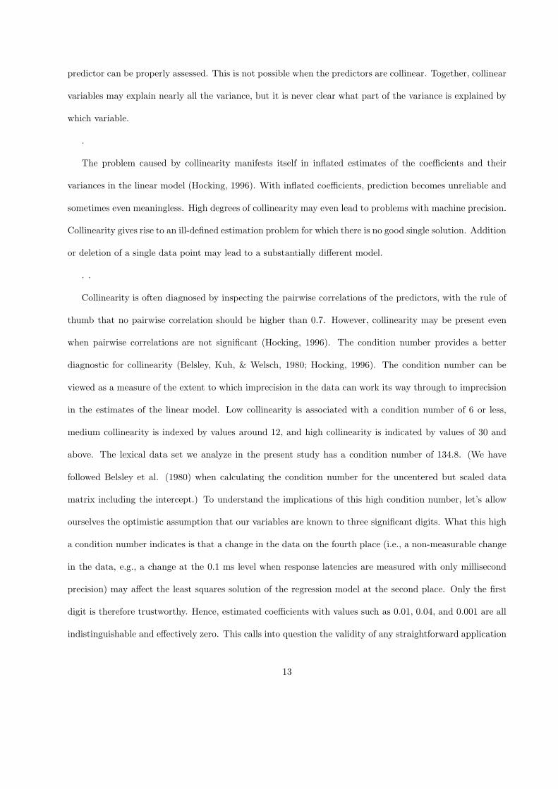
Figure 1 provides a graphical overview of the correlational structure of the full set of our predictors. We
first obtained the correlation matrix for the predictors using Spearman’s ρ. We squared the elements of this
matrix, to obtain a similarity metric that is sensitive to many types of dependence, including non-monotonic
relationships (cf. Harrell, 2001). The resulting similarity matrix was input to divisive hierarchical clustering.
Divisive clustering has the advantage of bringing out the main clusters in the data more clearly (cf. Venables
& Ripley, 2002, 317). All statistical analyses in this study were carried out using R (R Development Core
Team, 2005), the present cluster analysis was carried out using the module ’cluster’ (Rousseuuw, Struyf, &
Hubert, 2005).
Note that the measures for phonological and orthographic consistency as well as our orthographic and
17
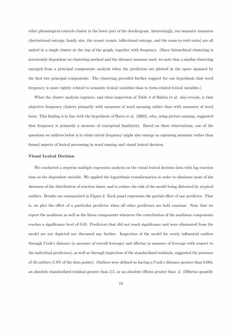
other phonological controls cluster in the lower part of the dendrogram. Interestingly, our semantic measures
(derivational entropy, family size, the synset counts, inflectional entropy, and the noun-to-verb ratio) are all
united in a single cluster at the top of the graph, together with frequency. (Since hierarchical clustering is
notoriously dependent on clustering method and the distance measure used, we note that a similar clustering
emerged from a principal components analysis when the predictors are plotted in the space spanned by
the first two principal components. The clustering provided further support for our hypothesis that word
frequency is more tightly related to semantic lexical variables than to form-related lexical variables.)
What the cluster analysis captures, and what inspection of Table 4 of Balota et al. also reveals, is that
objective frequency clusters primarily with measures of word meaning rather than with measures of word
form. This finding is in line with the hypothesis of Bates et al. (2003), who, using picture naming, suggested
that frequency is primarily a measure of conceptual familiarity. Based on these observations, one of the
questions we address below is to what extent frequency might also emerge as capturing semantic rather than
formal aspects of lexical processing in word naming and visual lexical decision.
Visual Lexical Decision
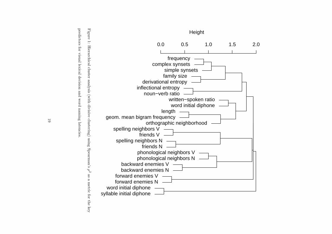
We conducted a stepwise multiple regression analysis on the visual lexical decision data with log reaction
time as the dependent variable. We applied the logarithmic transformation in order to eliminate most of the
skewness of the distribution of reaction times, and to reduce the risk of the model being distorted by atypical
outliers. Results are summarized in Figure 2. Each panel represents the partial effect of one predictor. That
is, we plot the effect of a particular predictor when all other predictors are held constant. Note that we
report the nonlinear as well as the linear components whenever the contribution of the nonlinear components
reaches a significance level of 0.05. Predictors that did not reach significance and were eliminated from the
model are not depicted nor discussed any further. Inspection of the model for overly influential outliers
through Cook’s distance (a measure of overall leverage) and dfbetas (a measure of leverage with respect to
the individual predictors), as well as through inspection of the standardized residuals, suggested the presence
of 43 outliers (1.9% of the data points). Outliers were defined as having a Cook’s distance greater than 0.005,
an absolute standardized residual greater than 2.5, or an absolute dfbeta greater than .2. (Dfbetas quantify
18
frequencycomplex synsets
simple synsetsfamily size
derivational entropyinflectional entropy
noun−verb ratiowritten−spoken ratioword initial diphone
lengthgeom. mean bigram frequency
orthographic neighborhoodspelling neighbors V
friends Vspelling neighbors N
friends Nphonological neighbors Vphonological neighbors N
backward enemies Vbackward enemies N
forward enemies Vforward enemies N
word initial diphonesyllable initial diphone
0.0 0.5 1.0 1.5 2.0
Height
Fig
ure
1:
Hiera
rchica
lclu
steranaly
sis(w
ithdiv
isive
clusterin
g)
usin
gSpea
rman’s
ρ2
as
am
etricfo
rth
ekey
pred
ictors
for
visu
allex
icaldecisio
nand
word
nam
ing
laten
cies.
19
the change in the estimated coefficient if an observation is excluded, relative to its standard error.) Examples
of outliers (as identified by the dfbetas) are jape, cox, cyst, skiff, broil, thwack, bloke, mum, nick, sub. The
estimates of the coefficients differed minimally from those of the model for the complete set of data points
(r = 0.9999). In what follows, we restrict ourselves to the model obtained after removal of the outliers.
The upper left panel shows the effect of the first principal component based on our consistency measures
(F (1, 2226) = 8.58, p = 0.0034), the only principal component that emerged as significant. Overall, the
consistency measures slowed decision latencies (all had positive loadings with this pc). Slowing was greater
for words with large phonological neighborhoods than for words with many feedforward enemies.
The second panel summarizes a small effect of whether the first phoneme of the word was voiced or
voiceless, as this variable was observed to be significant by Balota et al. (2004). In our analysis, it reached
significance as well (F (1, 2226) = 8.56, p = 0.0035). As pointed out by Balota and colleagues, this suggests
that the articulatory or phonological processes also codetermine lexical decision performance. The third
panel depicts the effect of the geometric mean bigram frequency. This measure, which is strongly correlated
with word length, was inhibitory (F (1, 2226) = 11.29, p = 0.0008).
The upper right panel of Figure 2 depicts the non-linear facilitatory effect of frequency (F (4, 2226) =
299.85, p < 0.0001; nonlinear: F (3, 2226) = 56.21, p < 0.0001). The non-linearity asymptotes in a floor
effect such that the facilitatory benefit of each additional log unit in frequency levels off as the limit of the
fastest possible response is approached. Note that the use of restricted cubic splines is revealing here. If we
would have used a quadratic term (as did Balota et al. (2004) in Figure 8), the resulting regression curve
would have suggested some slight inhibition for the highest frequencies, but this is just an artifact of using
a technique that is known not to work well for threshold effects such as the one we observe here.
The first panel on the second row represents the inhibitory effect of the written-to-spoken frequency
ratio (F (1, 2226) = 90.99, p < 0.0001). As the discrepancy between a word’s written and spoken frequency
increases, response latencies in the visual lexical decision task increase. Words that occur predominantly in
writing elicited longer response latencies in visual lexical decision than words that occur predominantly in
speech.
20
consistency (PC1)
log
RT
(m
s)
−6 −2 2 4 6
6.30
6.35
6.40
6.45
6.50
voice
log
RT
(m
s)
voiced voiceless
6.30
6.35
6.40
6.45
6.50
− −
−−
mean bigram frequency
log
RT
(m
s)
6 7 8 9 10
6.30
6.35
6.40
6.45
6.50
log frequency
log
RT
(m
s)
0 2 4 6 8 12
6.30
6.35
6.40
6.45
6.50
written−to−spoken ratio
log
RT
(m
s)
−3 −1 1 3
6.30
6.35
6.40
6.45
6.50
word category
log
RT
(m
s)
N V
6.30
6.35
6.40
6.45
6.50
−−
−−
noun−to−verb ratio
log
RT
(m
s)
−15 −5 0 5 10
6.30
6.35
6.40
6.45
6.50
derivational entropylo
g R
T (
ms)
0.0 1.0 2.0 3.0
6.30
6.35
6.40
6.45
6.50
log complex synsets
log
RT
(m
s)
0 1 2 3 4 5 6
6.30
6.35
6.40
6.45
6.50
inflectional entropy
log
RT
(m
s)
0.0 1.0 2.0
6.30
6.35
6.40
6.45
6.50
Figure 2: Partial effects of the predictors for lexical decision latencies (adjusted for nouns and for the medians
of the other covariates; 95% confidence intervals indicated by dashed lines).
21
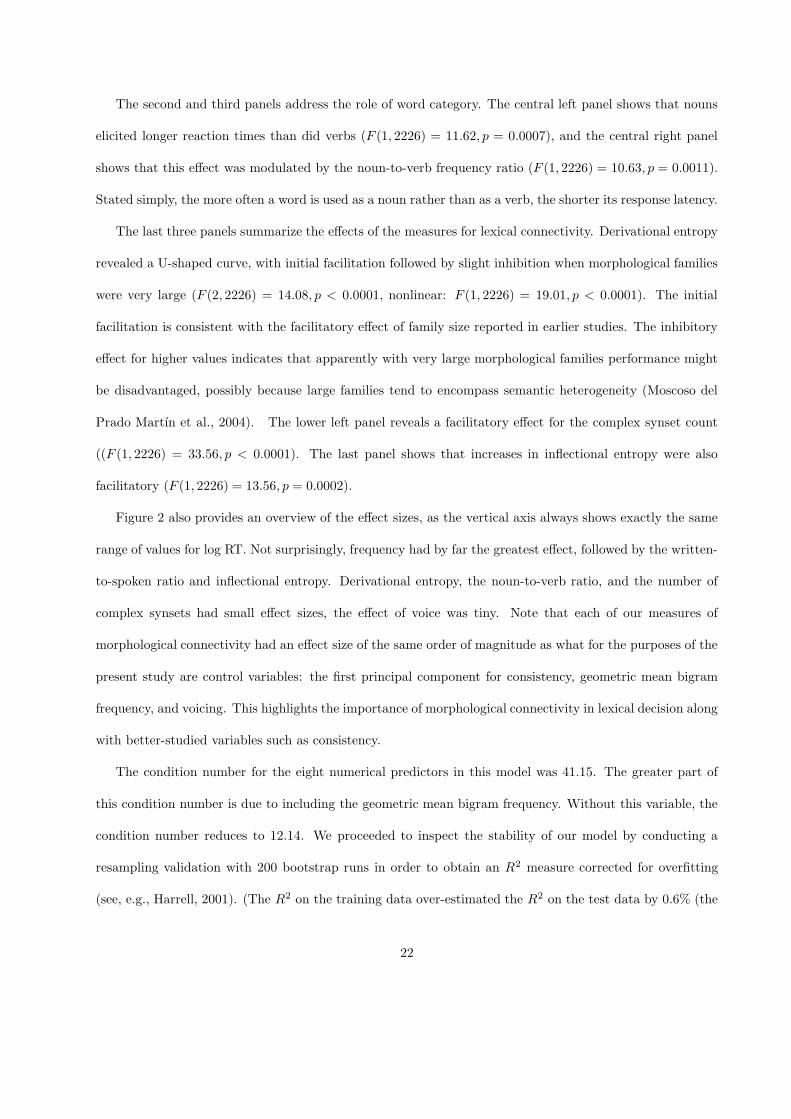
The second and third panels address the role of word category. The central left panel shows that nouns
elicited longer reaction times than did verbs (F (1, 2226) = 11.62, p = 0.0007), and the central right panel
shows that this effect was modulated by the noun-to-verb frequency ratio (F (1, 2226) = 10.63, p = 0.0011).
Stated simply, the more often a word is used as a noun rather than as a verb, the shorter its response latency.
The last three panels summarize the effects of the measures for lexical connectivity. Derivational entropy
revealed a U-shaped curve, with initial facilitation followed by slight inhibition when morphological families
were very large (F (2, 2226) = 14.08, p < 0.0001, nonlinear: F (1, 2226) = 19.01, p < 0.0001). The initial
facilitation is consistent with the facilitatory effect of family size reported in earlier studies. The inhibitory
effect for higher values indicates that apparently with very large morphological families performance might
be disadvantaged, possibly because large families tend to encompass semantic heterogeneity (Moscoso del
Prado Martın et al., 2004). The lower left panel reveals a facilitatory effect for the complex synset count
((F (1, 2226) = 33.56, p < 0.0001). The last panel shows that increases in inflectional entropy were also
facilitatory (F (1, 2226) = 13.56, p = 0.0002).
Figure 2 also provides an overview of the effect sizes, as the vertical axis always shows exactly the same
range of values for log RT. Not surprisingly, frequency had by far the greatest effect, followed by the written-
to-spoken ratio and inflectional entropy. Derivational entropy, the noun-to-verb ratio, and the number of
complex synsets had small effect sizes, the effect of voice was tiny. Note that each of our measures of
morphological connectivity had an effect size of the same order of magnitude as what for the purposes of the
present study are control variables: the first principal component for consistency, geometric mean bigram
frequency, and voicing. This highlights the importance of morphological connectivity in lexical decision along
with better-studied variables such as consistency.
The condition number for the eight numerical predictors in this model was 41.15. The greater part of
this condition number is due to including the geometric mean bigram frequency. Without this variable, the
condition number reduces to 12.14. We proceeded to inspect the stability of our model by conducting a
resampling validation with 200 bootstrap runs in order to obtain an R2 measure corrected for overfitting
(see, e.g., Harrell, 2001). (The R2 on the training data over-estimated the R2 on the test data by 0.6% (the
22
so-called optimism, an estimate of the extent to which we overestimate R2, and hence a measure of the degree
of overfitting), and the resulting bias-corrected R2 was 54.0%.) It is interesting to note that fast backward
elimination of predictors left all ten predictors in the model in 167 out of 200 bootstrap runs, removed one
predictor in 25 runs, and two predictors in 8 runs. In all, the resampling validation points to a robust and
reliable model that compares favorably to a model including the 24 original variables (and voicing) in our
database. For that model, the bootstrap-adjusted R2 was only 45.6%, with the modal number of predictors
retained at 9 (for only 49 bootstrap runs). We point out that because there was astronomical collinearity
among the total set of predictors (the condition number was 135), the more parsimonious model with lower
collinearity had superior explanatory power.
A parallel logistic regression model on the accuracy data revealed significance for the same set of predic-
tors, with similar functional relations (all p < 0.0001, z-tests on the coefficients), except for the voicing of
the initial phoneme, p = 0.0152). In addition, a small non-linear effect of length was present (p < 0.0001,
nonlinear: p = 0.0001), the increase in accuracy decreased slightly with increasing length. By contrast, our
analysis of the response latencies did not support word length as a significant independent predictor of visual
lexical decision latencies (p > 0.1). This finding contrasts with the results reported in two other studies,
Baayen (2005) and New, Ferrand, Pallier and Brysbaert (in press), both of which describe a non-linear,
U-shaped effect of length on visual lexical decision latencies. The former study (which made use of a less
comprehensive set of predictors) was based not only on the responses of the young age group (as the present
study) but also on those of the old age group. We therefore fitted the same statistical model to the response
latencies of the older subjects, using the same set of words. In contrast to what we observed for the younger
subjects, the partial effect of word length emerged as highly significant and non-linear (p < 0.0001, nonlinear:
p < 0.0001). This shows that the non-linear effect of length is characteristic of older, and potentially more
experienced, or possibly slower, readers. Apparently, the effect of word length is visible for the young readers
only in the accuracy measure.
The study by New et al. considered a much larger dataset including large numbers of polysyllabic and
morphologically complex words. For a subset of 4000 monomorphemic nouns, they report a curvilinear
23
effect of length as well. It is possible that with the increase in power due to the larger number of words
considered, an effect of length emerges in their data. On the other hand, further research may yield additional
insights. For instance, it is unclear from their study what the age of the subjects participating in the
underlying experiments was. Second, New et al. considered a highly restricted number of predictor variables
(printed frequency, number of syllables, and number of orthographic neighbors), and did not take variables
capturing orthographic consistency and aspects of a word’s morphological and semantic connectivity into
account. Given the complexity of multidimensional lexical space, regression analyses will need to be based
on comprehensive and overlapping sets of predictors. Otherwise, inconsistent results may ensue when the
same large databases are studied by different groups of researchers.
These considerations lead to the conclusion that great care and methodological rigor is required when
using large databases of response latencies, with respect to the subject groups included, with respect to the
kinds of items selected for analysis, and with respect to the predictors they include.
Balota et al. (2004) reported two interactions involving frequency that are of special interest: an inter-
action of frequency by Length, and an interaction of frequency by Neighborhood Density. When we added
these interactions to our model, we failed to detect any support for them. A fast backward elimination algo-
rithm removed all terms involving neighborhood density and length in letters from the model. The absence
of these interactions in our model and their presence in that of Balota et al. (2004) can be traced to their
using linear multiple regression. These authors were aware of the non-linear relation between frequency and
reaction time, as they modeled it by adding a quadratic term to a model regressing latency on frequency (see
their Figure 8). However, they did not incorporate this nonlinearity in their multiple regression analyses,
because (Balota and Yap, personal communication) they were concerned that including both interactions
and nonlinear terms would lead to instability in the regression equation (Cohen, Cohen, West, and Aiken,
2003: 299–300). No such concern is expressed in Harrell (2001), however. In fact, Harrell argues that predic-
tion accuracy may crucially depend on bringing nonlinearities into the model. Here we note that, as shown
in (our) Figure 2, there is a marked non-linearity in the partial effect of frequency even after the effect of
all other predictors has been taken into account. We also note that the a-priori imposition of linearity for
24
frequency leads to a loss in prediction accuracy: The goodness of fit of a model with a linear frequency effect
and an interaction of Neighborhood Density by Frequency (now significant, p = 0.0011) is inferior to the
model without this interaction but with a nonlinear effect of Frequency (adjusted R2 = 0.51 as compared to
R2 = 0.54). Since the model with the superior explanatory potential also validated well under the bootstrap,
instability in the regression equation does not seem to at issue for our data.
The statistical literature advises not to investigate interactions between numerical predictors, unless
there are theoretical reasons for doing so, see, e.g., page 33 in Harrell (2001). On the other hand, inter-
actions that are observed repeatedly may warrent further theoretical interpretation. For the visual lexical
decision latencies, we observed two significant interactions that we mention here for completeness. The
count of complex synsets entered into interactions with residualized familiarity (a measure introduced be-
low, F (1, 2223) = 23.32, p < 0.0001) and with inflectional entropy (F (1, 2223) = 14.92, p = 0.0001). In both
cases, the facilitatory effect of number of complex synsets was somewhat attenuated for higher values of
residualized familiarity and inflectional entropy. Including these interactions in the model did not lead to
substantial changes in the other predictors.
The hierarchical regression analysis of Balota et al. also led to the conclusion that Neighborhood Density
has a facilitatory effect on visual lexical decision latencies, in line with studies such as Andrews (1989) and
Forster & Shen (1996). Our analysis, however, did not reveal a significant effect of Neighborhood Density.
A principal components regression using the 24 original predictors likewise did not reveal an independent
contribution for this measure (p = 0.5864). Instead, it pointed to significant inhibitory effects of the spelling
neighbors and spelling friends (both p < 0.0001) with which the neighborhood count enters into a strong
correlation (r = 0.475 and r = 0.437 respectively). This suggests that the overall neighborhood density
measure has nothing to contribute once more sophisticated measures of spelling neighborhood sizes are taken
into account. It is noteworthy that the two consistency measures for neighborhood effects are both inhibitory
in the principal components regression, which is in line with the inhibitory effect of the first principal
component for our measures of orthographic consistency in our ordinary least squares model (correlation
with neighborhood density: r = 0.353). In other words, more sophisticated measures of neighborhood
25
density seem to indicate inhibition rather than facilitation. Addressing collinearity in a principled way may
therefore help to reconcile the puzzle of the inhibitory effect of neighborhood density reported for French
(Grainger, 1990, 1992; Grainger & Jacobs, 1996) and the facilitatory effect of neighborhood density reported
for English (Andrews, 1986, 1989, 1992, 1997). We leave the issue of potential differences across languages
and spelling systems for future clarification, and turn to the analysis of the naming data.
Word Naming
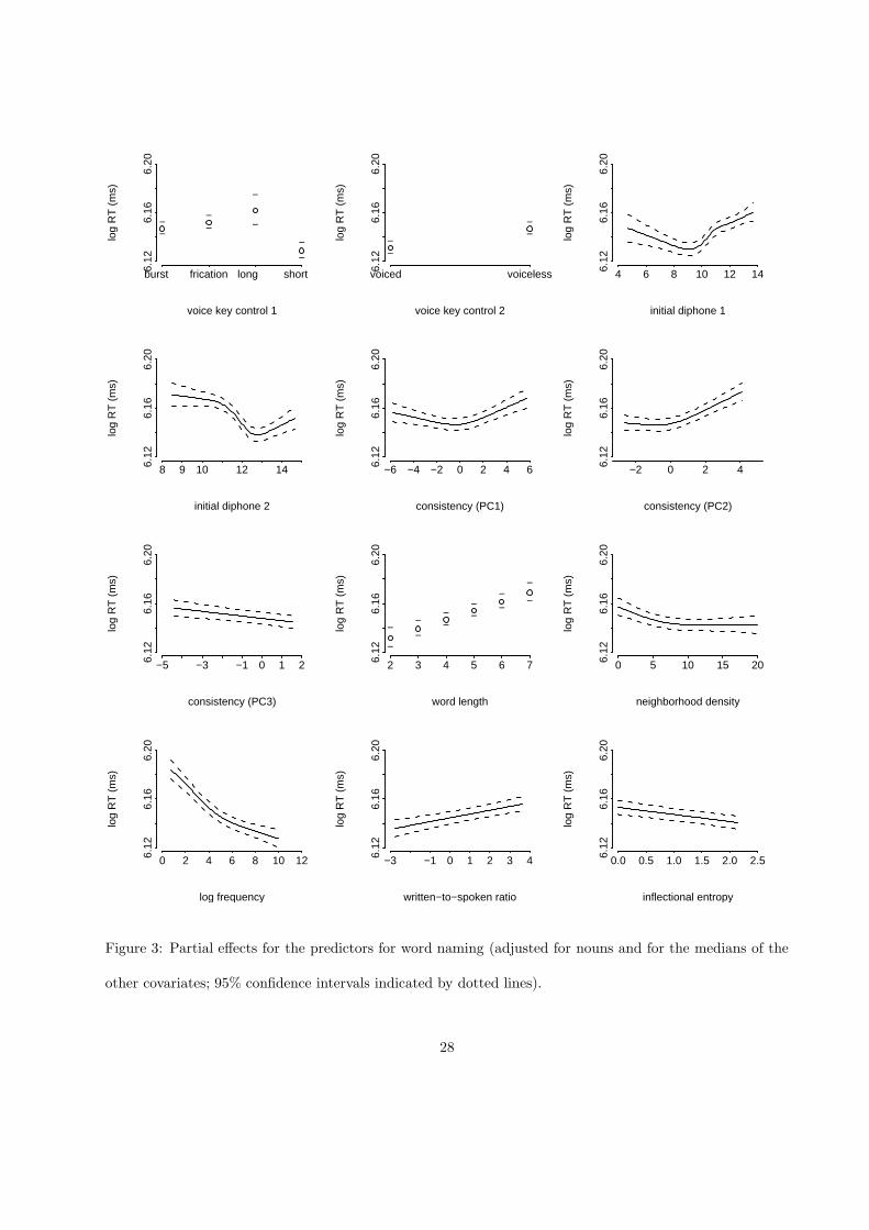
Figure 3 presents an overview of the predictors for naming latencies that remained in our stepwise
regression analysis. As in the analysis of the decision latencies, we inspected the model for outliers. Using
the same criteria, 59 outliers with undue leverage were identified and removed. Removal did not affect
whether predictors reached significance, but resulted in a tighter fit with more precise estimates for the
coefficients.
The first two panels on the top row concern the factors controlling for the effects of the voice key: the
presence of frication, bursts, and vowel length (F (3, 2206) = 33.57, p < 0.0001) and voicing (F (1, 2206) =
76.29, p < 0.0001). Collectively, these voice key variables accounted for 19.6% of the variance in the naming
latencies. As shown by Balota et al. (2004), a greater proportion of variance can be captured by including
a larger set of variables. We were reluctant to include many such variables, as this would have increased
the collinearity in our data matrix. For instance, whether the initial segment is voiced or voiceless is
predictable in a logistic regression model from inflectional entropy (p = 0.0041), the first principal component
of phonological consistency (p < 0.0001), and derivational entropy (p = 0.0537). Instead of adding additional
phonological voice key controls, we opted for using initial diphone frequencies as further quantitative controls.
The next two panels show the partial effects of the controls for the initial diphone. The third panel
on the top row shows the effect of the log frequency of the initial diphone, calculated over syllable-initial
positions. The first panel on the second row shows the effect of diphone frequency calculated over all positions.
Interestingly, the two measures are only weakly correlated (r = 0.12), and both contribute independently to
the model. Moreover, both show a marked U-shaped function, with initial facilitation followed by inhibition
(F (4, 2206) = 43.36, p < 0.0001, nonlinear: F (3, 2206) = 23.09, p < 0.0001, for the syllable-conditioned
26
measure; F (3, 2206) = 63.67, p < 0.0001, nonlinear: F (2, 2206) = 29.49, p < 0.0001 for the unconditional
count). Possibly, the inhibitory effect of frequent initial diphones reflects a trade-off between articulatory
ease (facilitatory) and costs of selection between other forms that begin with the same diphone.
The next three panels of Figure 3 show the partial effects for three (out of four) principal components that
represent the variables for orthographic consistency. The first principal component emerged with a u-shaped
function, unlike in visual lexical decision, where it was linear (F (1, 2206) = 22.17, p < 0.0001; nonlinear:
F (1, 2206) = 31.57, p < 0.0001). Apparently, not only larger but also smaller numbers of phonological and
spelling neighbors slow naming latencies. In addition, pc2 was mainly inhibitory (F (1, 2206) = 28.95, p <
0.0001; nonlinear: F (1, 2206) = 12.10, p = 0.004) and pc3 facilitatory (F (1, 2206) = 17.37, p = 0.0001).
More friends facilitated while more backward enemies inhibited (pc2), and the number of feedforward enemies
inhibited while the number of friends facilitated (pc3). The fourth principal component, which pulled apart
the type-based and token-based measures, was not significant.
Increases in word length (second panel on the third row) tended to slow naming as expected (F (1, 2206) =
52.01, p < 0.0001). Orthographic neighborhood density was facilitatory, but tended to asymptote quickly
(F (2, 2206) = 9.08, p = 0.0001, nonlinear: F (1, 2206) = 7.90, p = 0.0050), as can be seen in the last panel on
the third row of Figure 3.
The next two panels present two frequency effects. The effect of written frequency includes a small but
significant nonlinearity showing that it leveled off slightly for higher frequencies (F (2, 2206) = 143.91, p <
0.0001, nonlinear: (F1, 2206) = 13.95, p = 0.0002). Balota et al. did not observe such a nonlinearity for
naming, which may be due, first, to their use of a quadratic term (enforcing a specific functional form on the
curve) where we used splines, and second, to our analysis including covariates whereas Balota and colleagues
considered frequency by itself. The presence of this non-linearity and the similar form of this non-linearity
in visual lexical decision supports our interpretation of a floor effect — the closer one gets to the fastest
possible naming latency, the less the additional benefit of an additional log frequency unit is.
The contribution of the written to spoken frequency ratio that we observed for visual lexical decision also
emerged for naming latencies. As depicted in the center lower panel, words used predominantly in written
27
voice key control 1
log
RT
(m
s)
burst frication long short 6.12
6.16
6.20
− − −
−
−−
−
−
voice key control 2
log
RT
(m
s)
voiced voiceless6.12
6.16
6.20
−
−−
−
initial diphone 1
log
RT
(m
s)
4 6 8 10 12 146.12
6.16
6.20
initial diphone 2
log
RT
(m
s)
8 9 10 12 146.12
6.16
6.20
consistency (PC1)
log
RT
(m
s)
−6 −4 −2 0 2 4 66.12
6.16
6.20
consistency (PC2)
log
RT
(m
s)
−2 0 2 46.12
6.16
6.20
consistency (PC3)
log
RT
(m
s)
−5 −3 −1 0 1 26.12
6.16
6.20
word length
log
RT
(m
s)
2 3 4 5 6 76.12
6.16
6.20
−−
−−
−−
−−
−−
−−
neighborhood density
log
RT
(m
s)
0 5 10 15 206.12
6.16
6.20
log frequency
log
RT
(m
s)
0 2 4 6 8 10 126.12
6.16
6.20
written−to−spoken ratio
log
RT
(m
s)
−3 −1 0 1 2 3 46.12
6.16
6.20
inflectional entropy
log
RT
(m
s)
0.0 0.5 1.0 1.5 2.0 2.56.12
6.16
6.20
Figure 3: Partial effects for the predictors for word naming (adjusted for nouns and for the medians of the
other covariates; 95% confidence intervals indicated by dotted lines).
28
as contrasted with spoken English tended to have prolonged latencies (F (1, 2206) = 26.46, p < 0.0001).
The last panel summarizes the effect of inflectional entropy, which was also facilitatory as in visual lexical
decision (F (1, 2206) = 15.75, p = 0.0001). None of the other morphological variables were significant predic-
tors for the naming latencies. (Interactions of frequency by length and of frequency by neighborhood density
did not reach significance. When the nonlinear components are removed for frequency and neighborhood
density, a significant interaction of frequency by neighborhood density is observed, but the interaction of
frequency by length remains insignificant. The adjusted R2 of this model was 0.49, that of the simpler main
effects model with nonlinearities included was 0.50.)
Even for the present small number of predictors for the naming latencies, collinearity was quite high with
a condition number of 138.85. We therefore checked the validity of this model in two ways. First, we ran a
principal components regression. In this regression analysis, all our predictors were retained as significant
(p ≤ 0.001 except for pc3, p = 0.0537), and the directions of the effects were in correspondence with those
in Figure 3.
Second, we validated the model with 200 bootstrap resampling runs. In 196 runs, all predictors were
retained by a fast backward elimination algorithm, in 4 instances, 1 predictor was discounted. The optimism
for the R2 was 1.0%, and the bootstrap adjusted R2 was equal to 49.1%. As in our analysis of the lexical
decision data, the explanatory power of the parsimonious model with 12 predictors was superior, albeit
slightly, to a bootstrap-validated model including the 24 raw variables from our database (R2 = 41.1%. The
mode of the number of variables retained across the 200 runs for all variables was 14 and this occurred in
only 60 of the runs). We therefore conclude that the model summarized in Figure 3 is both parsimonious
and adequate.
A comparison of Figures 3 and 2 reveals, first of all, that most of the semantic predictors that are
significant for lexical decision are irrelevant for word naming. The greater sensitivity of visual lexical decision
to semantic variables is well known (Katz & Feldman, 1983; Lupker, 1979; Seidenberg & McClelland, 1989).
Nevertheless, the irrelevance for naming of word category, the noun-to-verb ratio, derivational entropy,
and the synset counts is remarkable, and suggests to us that the importance of word meaning is actually
29
substantially reduced in simple word naming compared to lexical decision.
Note that the effect size of word frequency in naming was roughly twice that of the other predictors, all
of which emerged with similarly sized effects. In lexical decision, the relative effect size of frequency was even
larger. The greater relative effect size in visual lexical decision as compared to word naming is consistent
with our intuition that a large part of the frequency effect captures semantic familiarity.
Ratings and Norms
In their analysis, Balota et al. (2004) included subjective frequency estimates as a predictor in their
multiple regression models for visual lexical decision and word naming latencies. In the light of Gernsbacher
(1984), this is not surprising: Subjective frequency estimates would be superior estimates of frequency of
occurrence compared to counts based on corpora. Moreover, Balota and colleagues’ aim was to partial out
any potential effects of frequency in order to be conservative with respect to their main goal, establishing
the importance of semantic variables over and above form variables.
We were hesitant to include subjective frequency ratings as a predictor in the preceding analyses, because
we had observed that measures other than frequency appear to predict subjective frequency ratings, see, e.g.,
Schreuder & Baayen (1997) and Balota, Pilotti & Cortese (2001). However rigid the methodology by means
of which subjective frequency ratings are solicited, they remain measures based on introspection, and we
have no guarantee whatsoever that these estimates are uncontaminated by other variables. Furthermore, as
we were interested in the unique explanatory potential of the individual predictors, including ratings would
be counterproductive and lead to increased collinearity, since the ratings themselves enter into functional
relationships with many of the other predictors.
In order to obtain evidence that subjective frequencies are an independent experimentally elicited variable
in their own right, whose status is analogous to that of visual lexical decision latencies or word naming
latencies, we studied the subjective frequency estimates in the Balota database with a stepwise regression
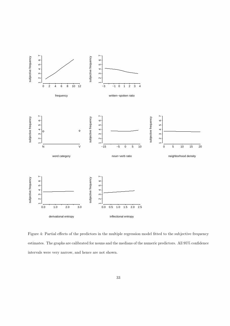
analysis, using the same predictors as in the preceding analyses. The predictors that emerged as significant
are summarized in Figure 4. As for the analyses of decision and naming latencies, we identified potentially
harmful outliers (51) on the basis of the initial analysis, and refitted the model to the reduced data set. As
30
for the naming data, removal of outliers did not lead to different conclusions, but allowed for more precise
estimates of the coefficients.
The upper left panel shows a nearly linear increase of the rating judgments with frequency (F (3, 2222) =
1548.20, p < 0.0001; nonlinear: F (2, 2222) = 6.56, p = 0.0014). It will come as no surprise that words
with greater frequencies elicited higher subjective frequency estimates. Interestingly, as shown by the next
figure, the effect of subjective frequency was modulated by the written to spoken frequency ratio, such that a
greater representation in written than in spoken English led to lower ratings (F (3, 2222) = 143.76, p < 0.0001,
nonlinear: F (2, 2222) = 6.90, p = 0.0010). This is reminiscent of the effect of the written-to-spoken ratio in
lexical decision and word naming, where a greater ratio led to longer latencies. Evidently, the role of spoken
frequency in studies of visual word recognition has been underestimated.
Of even greater interest are the remaining panels of Figure 4. The first two central panels show the
effects of word category. Nouns elicited slightly lower ratings than did verbs (left panel, F (1, 2222) =
11.19, p = 0.0008), although higher noun-to-verb ratios led to higher ratings (center panel, F (2, 2222) =
7.38, p = 0.0006, nonlinear: F (1, 2222) = 13.47, p = 0.0002). We leave it to the reader to verify that this
is the expected mirror image of what we observed for visual lexical decision. The third panel captures the
negative correlation between neighborhood density and the ratings (F (1, 2222) = 12.28, p = 0.0005). This
negative correlation is the flip side of the positive correlation observed for the first principal component for
consistency.
The panels on the bottom row summarize the positive correlations of the two entropy measures with the
ratings (derivational entropy: F (1, 2222) = 4.89, p = 0.0270, inflectional entropy: F (1, 2222) = 68.18, p <
0.0001). Their predictivity is in line with the results reported in Schreuder & Baayen (1997) for the simple
family size count. Note that the signs of the slopes of these effects are opposite to those in visual lexical
decision, just as is the case for frequency: longer lexical decision latencies correspond with lower subjective
frequency estimates. Thus, subjective frequency estimation emerges as a task that is in many ways the
off-line inverse of visual lexical decision. By implication, if subjective frequency estimates are included as a
predictor for other experimentally obtained dependent variables, it is crucial to first partial out the effects of
31
the related linguistic predictors. We will return to this issue below. The bootstrap-validated R2 of this model
was 0.756 — more than two thirds of the variance in the subjective ratings is predictable from ’objective’
lexical measures.
Age of Acquisition and Imageability
Subjective frequency ratings are not the only experimentally elicited variables that have been reified as
measures of lexical processing. In what follows, we will briefly touch upon two other such measures: age
of acquisition norms, and norms for imageability, as made available by Bird, Franklin, & Howard (2001).
These norms were available to us only for a small subset of the words in our database, and the results are
therefore more provisional compared to those based on the subjective frequency estimates.
The upper two rows of Figure 5 bring together the predictors for age of acquisition (shown on the vertical
axis) that reached significance in a stepwise multiple regression analysis of a subset of 336 words for which
we had at our disposal (a) age of acquisition norms, (b) imageability norms, and (c) the association norms
from the Florida database made available by Nelson, McEvoy, & Schreiber (1998). Nelson et al. (1998)
As in previous figures, the panels display the partial effects of the predictors, i.e., their effect when the
other predictors in the model are held constant. Greater values on the vertical axis denote an older age of
acquisition.
Not surprisingly, frequency and age of acquisition were negatively correlated (F (4, 324) = 22.85, p <
0.0001, nonlinear F (3, 324) = 5.18, p = 0.0017): Less frequent words are acquired later in life. The written-
to-spoken ratio showed a positive correlation (F (1, 324) = 40.33, p < 0.0001) such that words that appear
predominantly in writing tend to be learned later than words that are predominant in speech, which makes
sense as well.
The upper right panel shows that words with a greater inflectional entropy are learned earlier (F (4, 324) =
8.87, p < 0.0001, nonlinear: F (3, 324) = 3.17, p = 0.0245). Apparently, words with many inflectional variants,
and inflectional variants that are all used frequently, are acquired earlier in life.
The first panel on the second row shows the linear relation of imageability (or more precisely, residual
imageability, see below) and age of acquisition (F (1, 324) = 189.18, p < 0.0001). Not surprisingly, more
32
frequency
subj
ectiv
e fr
eque
ncy
0 2 4 6 8 10 12
12
34
56
7
written−spoken ratio
subj
ectiv
e fr
eque
ncy
−3 −1 0 1 2 3 4
12
34
56
7
word category
subj
ectiv
e fr
eque
ncy
N V
12
34
56
7
noun−verb ratio
subj
ectiv
e fr
eque
ncy
−15 −5 0 5 10
12
34
56
7
neighborhood density
subj
ectiv
e fr
eque
ncy
0 5 10 15 20
12
34
56
7
derivational entropy
subj
ectiv
e fr
eque
ncy
0.0 1.0 2.0 3.0
12
34
56
7
inflectional entropy
subj
ectiv
e fr
eque
ncy
0.0 0.5 1.0 1.5 2.0 2.5
12
34
56
7
Figure 4: Partial effects of the predictors in the multiple regression model fitted to the subjective frequency
estimates. The graphs are calibrated for nouns and the medians of the numeric predictors. All 95% confidence
intervals were very narrow, and hence are not shown.
33
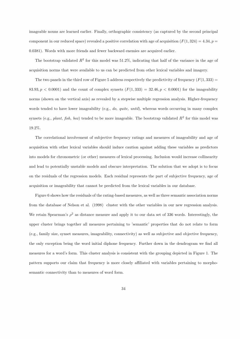
imageable nouns are learned earlier. Finally, orthographic consistency (as captured by the second principal
component in our reduced space) revealed a positive correlation with age of acquisition (F (1, 324) = 4.34, p =
0.0381). Words with more friends and fewer backward enemies are acquired earlier.
The bootstrap validated R2 for this model was 51.2%, indicating that half of the variance in the age of
acquisition norms that were available to us can be predicted from other lexical variables and imagery.
The two panels in the third row of Figure 5 address respectively the predictivity of frequency (F (1, 333) =
83.93, p < 0.0001) and the count of complex synsets (F (1, 333) = 32.46, p < 0.0001) for the imageability
norms (shown on the vertical axis) as revealed by a stepwise multiple regression analysis. Higher-frequency
words tended to have lower imageability (e.g., do, quite, until), whereas words occurring in many complex
synsets (e.g., plant, fish, box) tended to be more imageable. The bootstrap validated R2 for this model was
19.2%.
The correlational involvement of subjective frequency ratings and measures of imageability and age of
acquisition with other lexical variables should induce caution against adding these variables as predictors
into models for chronometric (or other) measures of lexical processing. Inclusion would increase collinearity
and lead to potentially unstable models and obscure interpretation. The solution that we adopt is to focus
on the residuals of the regression models. Each residual represents the part of subjective frequency, age of
acquisition or imageability that cannot be predicted from the lexical variables in our database.
Figure 6 shows how the residuals of the rating-based measures, as well as three semantic association norms
from the database of Nelson et al. (1998) cluster with the other variables in our new regression analysis.
We retain Spearman’s ρ2 as distance measure and apply it to our data set of 336 words. Interestingly, the
upper cluster brings together all measures pertaining to ’semantic’ properties that do not relate to form
(e.g., family size, synset measures, imageability, connectivity) as well as subjective and objective frequency,
the only exception being the word initial diphone frequency. Further down in the dendrogram we find all
measures for a word’s form. This cluster analysis is consistent with the grouping depicted in Figure 1. The
pattern supports our claim that frequency is more closely affiliated with variables pertaining to morpho-
semantic connectivity than to measures of word form.
34
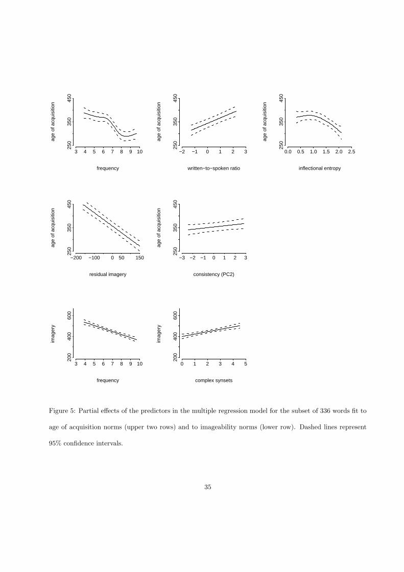
frequency
age
of a
cqui
sitio
n
3 4 5 6 7 8 9 10
250
350
450
written−to−spoken ratio
age
of a
cqui
sitio
n−2 −1 0 1 2 3
250
350
450
inflectional entropy
age
of a
cqui
sitio
n
0.0 0.5 1.0 1.5 2.0 2.5
250
350
450
residual imagery
age
of a
cqui
sitio
n
−200 −100 0 50 150
250
350
450
consistency (PC2)
age
of a
cqui
sitio
n
−3 −2 −1 0 1 2 3
250
350
450
frequency
imag
ery
3 4 5 6 7 8 9 10
200
400
600
complex synsets
imag
ery
0 1 2 3 4 5
200
400
600
Figure 5: Partial effects of the predictors in the multiple regression model for the subset of 336 words fit to
age of acquisition norms (upper two rows) and to imageability norms (lower row). Dashed lines represent
95% confidence intervals.
35
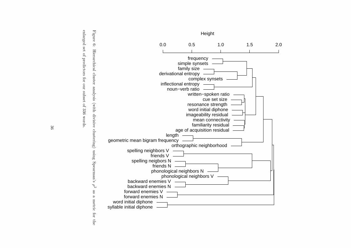
frequencysimple synsetsfamily size
derivational entropycomplex synsets
inflectional entropynoun−verb ratio
written−spoken ratiocue set size
resonance strengthword initial diphone
imageability residualmean connectivityfamiliarity residual
age of acquisition residuallength
geometric mean bigram frequencyorthographic neighborhood
spelling neighbors Vfriends V
spelling neigbors Nfriends N
phonological neighbors Nphonological neighbors V
backward enemies Vbackward enemies N
forward enemies Vforward enemies N
word initial diphonesyllable initial diphone
0.0 0.5 1.0 1.5 2.0
Height
Fig
ure
6:
Hiera
rchica
lclu
steranaly
sis(w
ithdiv
isive
clusterin
g)
usin
gSpea
rman’s
ρ2
as
am
etricfo
rth
e
enla
rged
setofpred
ictors
for
our
subset
of336
word
s.36

In a final series of analyses, we addressed the explanatory potential of the three residualized measures
for the chronometric measures. First we considered the full data set, to which we added the residuals for the
subjective frequency ratings as a new predictor.
When we added the residual subjective frequency rating to the model for lexical decision, there was a
large and significant effect (F (1, 2220) = 186.43, p < 0.0001), such that the higher (residual) ratings led to
shorter visual lexical decision latencies, as expected. The bootstrap-validated R2 for this model was 57.6%
(as compared with the original bootstrap-validated R2 of 53.8% reported above). The implication is that
the subjective frequency rating is a powerful variable in its own right, even after the lexical covariates that
codetermine this subjective measure have been properly partialled out. The residual rating also contributed
to explaining the naming latencies (F (1, 2211) = 15.60, p = 0.0001), but led to only a tiny increase in the
bootstrap-validated R2, an increase from 48.3% to 48.8%. The other predictors in these two models were
only minimally affected. Summing up, residual subjective frequency estimates are more predictive for visual
lexical decision than for naming. Given that visual lexical decision is more sensitive to semantic variables
than is word naming, this finding strongly suggests that subjective frequency estimates are more sensitive
to semantic familiarity than to form familiarity.
Finally, we selected the predictors that were significant in the model fitted to the full data set and
supplemented them with the three residualized predictors along with the three association measures from
the Florida database that were available to us for the smaller data set. When we conducted stepwise
regression analyses on this smaller data set composed of 336 words, the only new variable that exerted
an effect was residual imageability on lexical decision latencies (F (1, 329) = 10.80, p < 0.0011). Moreover,
variables such as the written-spoken ratio, the noun-verb ratio, and inflectional entropy remained significant
for this smaller data set of decision latencies. Importantly, age of acquisition did not. From this we infer
that a properly residualized measure of age of acquisition is unlikely to lead to substantial changes in the
models that we obtained for the full data sets.
37
General Discussion
The main goal of the present study was to gauge the importance of morphological measures as well as
frequency in the lexical processing of morphologically simple words by means of a regression analysis on
the by-item latencies of the young participants in the visual lexical decision and word naming experiments
made available by Balota and his colleagues (Balota, Cortese, & Pilotti, 1999; Spieler & Balota, 1998). This
study therefore extends the seminal study of Balota, Cortese, Sergent Marschall, Spieler, & Yap (2004) by
considering a number of morphological variables that they did not consider in their analyses. Our primary
finding is that we see the new morphological variables of inflectional and derivational entropy at work in
visual lexical decision, each with effect sizes that are at least as large as that of the single form variable
(orthographic consistency) that remained significant in a stepwise modeling procedure. In addition we
observed a special role for spoken frequency. In word naming, by contrast, the only morphological variable
that retained the status of a significant predictor was inflectional entropy.
Table 1 lists for each significant predictor a lower bound for the percentage of variance accounted for
by that predictor. These percentages were computed by comparing the adjusted R2 of the full model with
the adjusted R2 of that model after removal of the predictor. For word naming, for instance, the R2 of the
full model was 0.4999. Removal of frequency reduced the R2 to 0.4391, hence the percentage of variance
uniquely accounted for by frequency over and above all other predictors is 6.08.
Table 1 is revealing in that it shows unambiguously that the unique contributions of many individual
predictors is minute, even though their presence in the model is justified statistically. Considered jointly,
the total amount of variance that we can attribute uniquely to specific predictors is roughly half of the
total amount of variance captured by the models (R2 = 0.4999 for naming, R2 = 0.5771 for visual lexical
decision). This is a consequence of the high collinearity characteristic of lexical space.
38
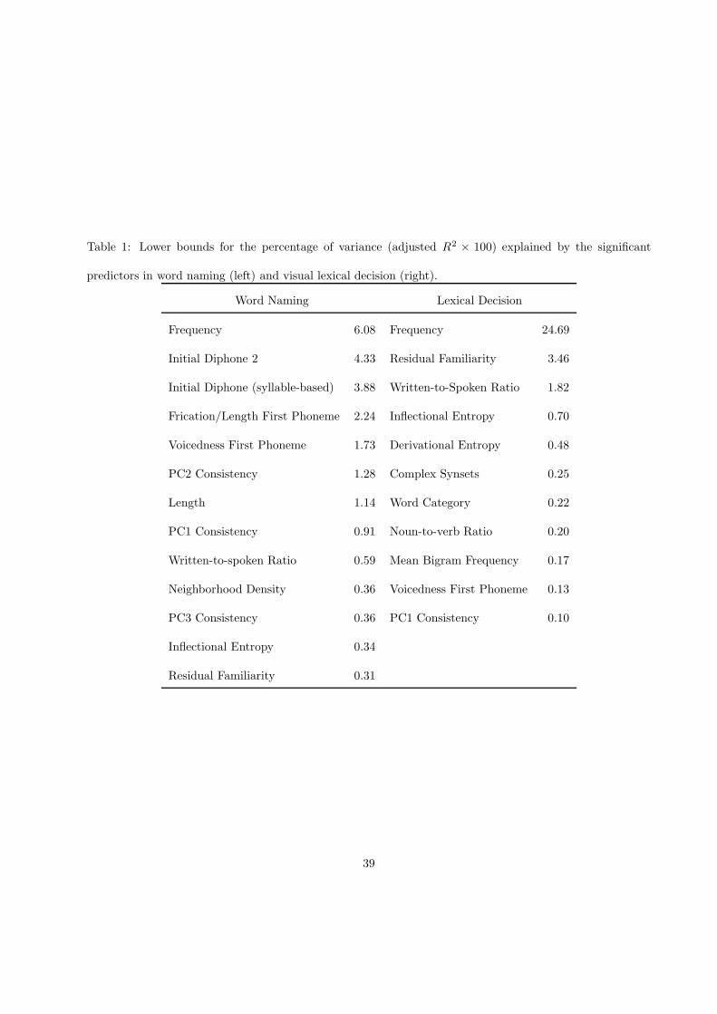
Table 1: Lower bounds for the percentage of variance (adjusted R2 × 100) explained by the significant
predictors in word naming (left) and visual lexical decision (right).
Word Naming Lexical Decision
Frequency 6.08 Frequency 24.69
Initial Diphone 2 4.33 Residual Familiarity 3.46
Initial Diphone (syllable-based) 3.88 Written-to-Spoken Ratio 1.82
Frication/Length First Phoneme 2.24 Inflectional Entropy 0.70
Voicedness First Phoneme 1.73 Derivational Entropy 0.48
PC2 Consistency 1.28 Complex Synsets 0.25
Length 1.14 Word Category 0.22
PC1 Consistency 0.91 Noun-to-verb Ratio 0.20
Written-to-spoken Ratio 0.59 Mean Bigram Frequency 0.17
Neighborhood Density 0.36 Voicedness First Phoneme 0.13
PC3 Consistency 0.36 PC1 Consistency 0.10
Inflectional Entropy 0.34
Residual Familiarity 0.31
39
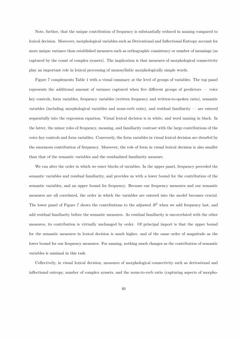
Note, further, that the unique contribution of frequency is substantially reduced in naming compared to
lexical decision. Moreover, morphological variables such as Derivational and Inflectional Entropy account for
more unique variance than established measures such as orthographic consistency or number of meanings (as
captured by the count of complex synsets). The implication is that measures of morphological connectivity
play an important role in lexical processing of monosyllabic morphologically simple words.
Figure 7 complements Table 1 with a visual summary at the level of groups of variables. The top panel
represents the additional amount of variance captured when five different groups of predictors — voice
key controls, form variables, frequency variables (written frequency and written-to-spoken ratio), semantic
variables (including morphological variables and noun-verb ratio), and residual familiarity — are entered
sequentially into the regression equation. Visual lexical decision is in white, and word naming in black. In
the latter, the minor roles of frequency, meaning, and familiarity contrast with the large contributions of the
voice key controls and form variables. Conversely, the form variables in visual lexical decision are dwarfed by
the enormous contribution of frequency. Moreover, the role of form in visual lexical decision is also smaller
than that of the semantic variables and the residualized familiarity measure.
We can alter the order in which we enter blocks of variables. In the upper panel, frequency preceded the
semantic variables and residual familiarity, and provides us with a lower bound for the contribution of the
semantic variables, and an upper bound for frequency. Because our frequency measures and our semantic
measures are all correlated, the order in which the variables are entered into the model becomes crucial.
The lower panel of Figure 7 shows the contributions to the adjusted R2 when we add frequency last, and
add residual familiarity before the semantic measures. As residual familiarity is uncorrelated with the other
measures, its contribution is virtually unchanged by order. Of principal import is that the upper bound
for the semantic measures in lexical decision is much higher, and of the same order of magnitude as the
lower bound for our frequency measures. For naming, nothing much changes as the contribution of semantic
variables is minimal in this task.
Collectively, in visual lexical decision, measures of morphological connectivity such as derivational and
inflectional entropy, number of complex synsets, and the noun-to-verb ratio (capturing aspects of morpho-
40
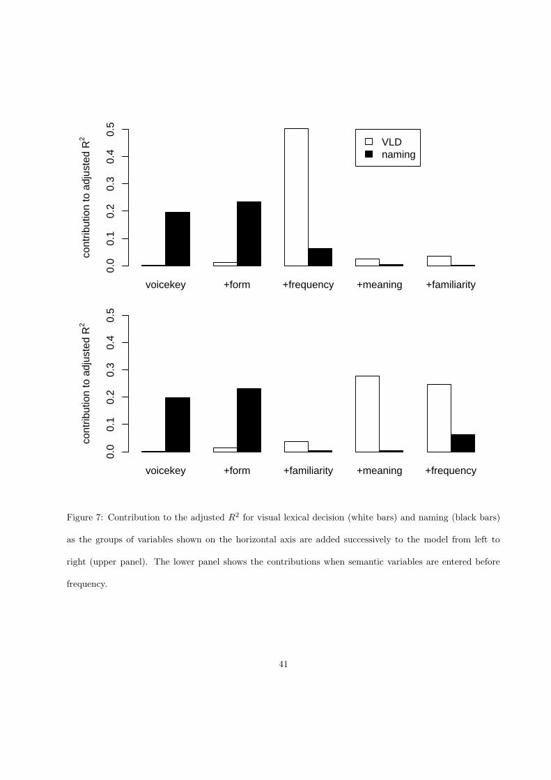
voicekey +form +frequency +meaning +familiarity
0.0
0.1
0.2
0.3
0.4
0.5
cont
ribut
ion
to a
djus
ted
R2 VLD
naming
voicekey +form +familiarity +meaning +frequency
0.0
0.1
0.2
0.3
0.4
0.5
cont
ribut
ion
to a
djus
ted
R2
Figure 7: Contribution to the adjusted R2 for visual lexical decision (white bars) and naming (black bars)
as the groups of variables shown on the horizontal axis are added successively to the model from left to
right (upper panel). The lower panel shows the contributions when semantic variables are entered before
frequency.
41
logical conversion) are predictors that jointly are, at a minimum, at least as important as measures of word
form. At best they are equally as explanatory as the word frequency effect itself. Finally, there was no
independent predictivity from the simple synset count. The implication is that a word’s morphological
connectivity rather than a word’s number of morphologically unrelated synonyms emerges as the primary
semantic factor in visual lexical decision.
In this study, we have demonstrated some of the problems that the reification of subjective estimates,
whether of frequency, age of acquisition, or imageability can introduce. For instance, subjective frequency
in and of itself is a dependent variable that is to a large extent (bootstrap-validated R2 = 0.76) predictable
from other lexical measures (see also Balota, Pilotti & Cortese, 2001). For subjective estimates of age
of acquisition, roughly half of the variance could be traced to lexical predictors and imageability, and for
subjective measures of imageability, it was the case that one fifth of the variance could be explained. For
the subset of the data for which we had age of acquisition norms, the written-to-spoken ratio turned out
to be predictive in lexical decision to the exclusion of (residualized) age of acquisition. For larger datasets,
however, it may be that age of acquisition emerges as an independent predictor as well (De Jong, 2002).
While subjective frequency has a high correlation with the decision latencies (r = −0.67), partialling out
the lexical predictors reduces this correlation to r = −0.20, which amounts to a drop from 44.9% to a mere
4.1% of variance explained. This small contribution also is evident in Figure 7. Balota et al. (2004:311)
argued that their young subjects appeared ”to have good metacognitive insights into their frequency of
exposure to words.” Our findings suggest another interpretation. Rather than claim that introspection
provides access to frequency of exposure, subjective frequency estimates may be determined largely by
the same variables that predict visual lexical decision latencies. In essence, subjective frequency estimates
are contaminated, or enriched, by measures of morphological connectivity, as well as by the written-to-
spoken ratio. The finding that in the regression a higher written frequency leads to lower instead of higher
subjective estimates means that it is unlikely that participants are able to access the frequency with which
they have encountered a word in written form. Although they might be tapping into the frequency with
which they have encountered the word in spoken form, our preferred interpretation is that they are guided
42
by conceptual familiarity. In support of our claim, we observed that residualized familiarity clustered with
semantic variables, not with measures of word form (see Figure 6).
We reiterate that both objective and subjective frequency cluster with semantic measures, including
measures for morphological connectivity. What are the implications of this observation for the more general
question of what is captured by frequency of occurrence? Balota & Chumbley (1984) and Balota et al. (2004)
have shown that visual lexical decision is sensitive to more than aspects of a word’s form. The results from
the present study are consistent with this view, but invite a more extreme position, according to which in
visual lexical decision frequency reflects primarily conceptual familiarity. Even though frequency (or rank)
might still be a guiding principle for lexical access, as argued by Murray and Forster (2004), we have several
reasons for pursuing the claim that frequency is a far more important organizational principle at the semantic
level.
Not only is it unlikely that word frequency would primarily tap into formal levels of representation and
processing given the structure of lexical space, it is the case that the gain in predictive accuracy by adjusting
for the frequency of use in speech rather than in writing (by means of the written-to-spoken ratio) also argues
against locating the frequency effect primarily at the level of visual access. The persistance of frequency
effects in reading across changes in font (Allen, Wallace, & Weber, 1995) provides further evidence for this
position.
Furthermore, we have demonstrated that frequency is an important predictor for imagery, for age-of-
acquisition, and for subjective frequency estimates. In essence, frequency is highly correlated with a number
of variables that have no immediate relation with the familiarity of a word’s orthographic form. Whenever
frequency is varied, these variables will tend to covary.
The reduction in the explanatory power of the frequency effect illustrated in Figure 7 that results from
partialing out the effect of established semantic variables provides further support for the tight relation
between frequency and semantics. In fact, the naming data suggest an upper bound for the extent to which
frequency reflects form-based processing. Given that word naming combines visual perception with speech
43
production, there are two levels at which form representations can be involved, at the input and at the
output levels. The combined form frequency effects at these two levels apparently contribute less than 10%
to the explained variance. This is an upper limit, as we cannot exclude the possibility that meaning (and
concomitant frequency-driven processing) was involved during naming.
Finally, the frequency effect was modulated by the noun-to-verb ratio. Conversion pairs such as the/to
work share the same form, and nevertheless the frequencies with which they are used as a noun or as a verb
are reflected in visual lexical decision latencies, see also Feldman and Basnight-Brown (2005). This cannot
be explained in terms of properties of the word’s orthographic form.
In addition to insights into the semantic nature of the frequency effect, the present study also offers a
methodological advance. It illustrates the advantages of regression with restricted cubic splines to model
nonlinearities. Serious consideration of non-linearities is an absolute prerequisite for accurate prediction
(Harrell, 2001), even when there are no immediate, self-evident explanations available. For instance, we
observed U-shaped nonlinear relations in both visual lexical decision and in naming, for which we could
offer only tentative explanations in terms of conflicting constraints. Obviously, further research is required
here because we have also illustrated how spurious interactions may arise if non-linearities are not properly
brought into the model.
The present study also called attention to the dangers of collinearity and suggested some simple strategies
to address these dangers. The models that we presented were both economical and superior in predictivity
to models including many more collinear variables.
In summary, our analysis fully supports the conclusion reached by Balota and colleagues that in visual
lexical decision semantic factors are predictive over and above frequency and measures of a word’s form.
We have extended their work by showing that a series of morphological variables — variables for which
we have independent evidence that they are semantic in nature — are also co-determining visual lexical
decision latencies over and above measures of a word’s form properties. We have taken their approach a step
further by arguing that in visual lexical decision, word frequency itself is a measure that captures primarily
44
semantics rather than word form, for instance, by showing that a higher spoken frequencies correlate with
shorter reaction times in visual lexical decision. Our analysis diverges from that of Balota and colleagues
with respect to the interactions of word frequency by length and neighborhood density, which turn out not
to be necessary once the nonlinear nature of the frequency effect is brought into the model for visual lexical
decision.
To conclude, we offer a final insight into the implications of the high collinearity of measures of lexical
processing for theories of the mental lexicon. In our statistical analysis, we invested in reducing collinearity
in order to ascertain whether our key variables are actually predictive independent of the other variables.
This does not imply, however, that we think these key variables are truly separable in lexical processing.
Rather, they capture aspects of a system that is characterized by high degrees of interconnectivity. This
interconnectivity can be modeled by distributed mappings between orthographic, phonological and semantic
representations, as in, for example, the triangle model (Seidenberg & Gonnerman, 2000; Harm & Seidenberg,
2004). In these models, storage is superpositional, and frequency affects the interconnectivity of nodes within
the network. Alternatively, interconnectivity can be modeled in exemplar based theories with localist repre-
sentations embedded in highly interconnected networks (Bybee, 2001; Hay & Baayen, 2005). In both cases,
the effect of word frequency need not be limited only to the word itself, but also affects its interconnections
with other units in the network.
. .
In both approaches, these are highly complex systems for which it may well be unrealistic to try to isolate
the effect of one specific lexical measure. Our predictors offer but crude quantifications of aspects of these
complex systems. None of our predictors take the complexity of the system into account in a principled
way. The price we pay for the crudeness of our measures is rampant collinearity. The flip side is that this
collinearity may itself be an index of the interconnectivity of the complex systems that we study. This
interconnectivity may actually be fundamental to the robustness that characterizes lexical processing. From
this perspective, the clustering of lexical measures that we have documented in the present study is the
signature of the extensive covariation between the many formal and semantic properties that characterize
45
the denizens of the mental lexicon. If this metaphor contains a grain of truth, then the role of morphological
connectivity and of word frequency are intertwined to an even greater degree than we have heretofore
envisioned.
46
Author note:
This research was supported in part by grant NIH HD-01994 to Haskins Laboratories.
47
References
Allen, P., Wallace, B., and Weber, T. (1995). Instance-based learning algorithms. Journal of Experimental
Psychology: Human perception and performance, 21, 914–934.
Andrews, S. (1986). Morphological influences on lexical access: lexical or non-lexical effects? Journal of
Memory and Language, 25, 726–740.
Andrews, S. (1989). Frequency and neighborhood size effects on lexical access: Activation or search? Journal
of Experimental Psychology: Learning, Memory, and Cognition, 15, 802–814.
Andrews, S. (1992). Frequency and neighborhood effects on lexical access: Lexical similarity or orthographic
redundancy? Journal of Experimental Psychology: Learning, Memory, & Cognition, 18, 234–254.
Andrews, S. (1997). The effects of orthographic similarity on lexical retrieval: Resolving neighborhood
conflicts. Psychological Bulletin & Review, 4, 439–461.
Baayen, R. (2005). Data mining at the intersection of psychology and linguistics. In A. Cutler (Ed.),
Twenty-first century psycholinguistics: Four cornerstones (pp. 69–83). Hillsdale, New Jersey: Erlbaum.
Baayen, R. H. (2001). Word Frequency Distributions. Kluwer Academic Publishers, Dordrecht.
Baayen, R. H. and Moscoso del Prado Martın, F. (2005). Semantic density and past-tense formation in three
Germanic languages. Language, 81, 666–698.
Baayen, R. H., Piepenbrock, R., and Gulikers, L. (1995). The CELEX lexical database (CD-ROM). Linguistic
Data Consortium, University of Pennsylvania, Philadelphia, PA.
Balota, D., Cortese, M., and Pilotti, M. (1999). Visual lexical decision latencies for 2906 words. [On-line],
Available: http://www.artsci.wustl.edu/∼dbalota/lexical decision.html.
Balota, D., Cortese, M., Sergent-Marshall, S., Spieler, D., and Yap, M. (2004). Visual word recognition for
single-syllable words. Journal of Experimental Psychology:General, 133, 283–316.
48
Balota, D. A. and Chumbley, J. I. (1984). Are lexical decisions a good measure of lexical access? The role of
word frequency in the neglected decision stage. Journal of Experimental Psychology: Human Perception
and Performance, 10, 340–357.
Balota, D. A., Pilotti, M., and Cortese, M. J. (2001). Subjective frequency estimates ofr 2,938 monosyllabic
words. Memory & Cognition, 29, 639–647.
Barry, C., Hirsh, K., Johnston, R. A., and Williams, C. (2001). Age of acquisition, word frequency, and the
locus of repetition priming of picture naming. Journal of memory and language, 44, 350–375.
Bates, E., D’Amico, S., Jacobsen, T., Szekely, A., Andonova, E., Devescovi, A., Herron, D., Ching Lu, C.,
Pechmann, T., Pleh, C., Wicha, N., Federmeier, K., Gerdjikova, I., Gutierrez, G., Hung, D., Hsu, J., Iyer,
G., Kohnert, K., Mehotcheva, T., Orozco-Figueroa, A., Tzeng, A., and Tzeng, O. (2003). Timed picture
naming in seven languages. Psychonomic Bulletin and Review, 10, 344–380.
Beckwith, R., Fellbaum, C., Gross, D., and Miller, G. (1991). WordNet: A lexical database organized on
psycholinguistic principles. In U. Zernik (Ed.), Lexical Acquisition. Exploiting On-Line Resources to Build
a Lexicon (pp. 211–232). Hillsdale, NJ: Lawrence Erlbaum Associates.
Belsley, D. A., Kuh, E., and Welsch, R. E. (1980). Regression Diagnostics. Identifying Influential Data and
sources of Collinearity. Wiley Series in Probability and Mathematical Statistics. Wiley, New York.
Bertram, R., Baayen, R. H., and Schreuder, R. (2000). Effects of family size for complex words. Journal of
Memory and Language, 42, 390–405.
Biber, D. (1988). Variation across speech and writing. Cambridge University Press, Cambridge.
Biber, D. (1995). Dimensions of register variation. Cambridge University Press, Cambridge.
Bird, H., Franklin, S., and Howard, D. (2001). Age of acquisition and imageability ratings for a large set of
words, including verbs and function words. Behavior Research Methods, Instruments, and Computers, 33,
73–79.
49
Brysbaert, M. (1996). Word frequency affects naming latency in Dutch with age-of-acquisition controlled.
European Journal of Cognitive Psychology, 8, 185–193.
Brysbaert, M., Lange, M., and Van Wijnendaele, I. (2000a). The effects of age-of-acquisition and frequency-
of-occurence in visual word recognition: Further evidence from the Dutch language. European Journal of
Cognitive Psychology, 12, 65–85.
Burnard, L. (1995). Users guide for the British National Corpus. British National Corpus consortium,
Oxford university computing service.
Bybee, J. L. (2001). Phonology and language use. Cambridge University Press, Cambridge.
Carroll, J. B. (1967). On sampling from a lognormal model of word frequency distribution. In H. Kucera and
W. N. Francis (Eds.), Computational Analysis of Present-Day American English (pp. 406–424). Providence:
Brown University Press.
Carroll, J. B. and White, M. N. (1973a). Age of acquisition norms for 220 picturable nouns. Journal of
Verbal Learning and Verbal Behavior, 12, 563–576.
Carroll, J. B. and White, M. N. (1973b). Word frequency and age of acquisition as determiners of picture-
naming latency. Quaterly Journal of Experimental Psychology, 25, 85–95.
Chatterjee, S., Hadi, A.S., and Price, B. (2000). Regression analysis by example. New York: John Wiley &
Sons.
Cohen, J., Cohen, P., West, S. G. and Aiken, L. S. (2003). Applied multiple regression/correlation analysis
for the behavioral sciences. Hillsdale, New Jersey: Lawrence Erlbaum Associates.
Coltheart, M., Davelaar, E., Jonasson, J. T., and Besner, D. (1977). Access to the internal lexicon. In S.
Dornick (Ed.), Attention and performance, volume VI (pp. 535–556). Hillsdale, New Jersey: Erlbaum.
Cortese, M. and Fugett, A. (2004). Imageability ratings for 3000 monosyllabic words. Behavioral methods
and research, instrumentation, & computers, 36, 384–387.
50
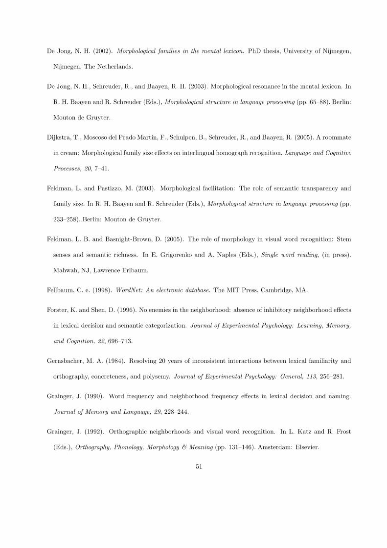
De Jong, N. H. (2002). Morphological families in the mental lexicon. PhD thesis, University of Nijmegen,
Nijmegen, The Netherlands.
De Jong, N. H., Schreuder, R., and Baayen, R. H. (2003). Morphological resonance in the mental lexicon. In
R. H. Baayen and R. Schreuder (Eds.), Morphological structure in language processing (pp. 65–88). Berlin:
Mouton de Gruyter.
Dijkstra, T., Moscoso del Prado Martın, F., Schulpen, B., Schreuder, R., and Baayen, R. (2005). A roommate
in cream: Morphological family size effects on interlingual homograph recognition. Language and Cognitive
Processes, 20, 7–41.
Feldman, L. and Pastizzo, M. (2003). Morphological facilitation: The role of semantic transparency and
family size. In R. H. Baayen and R. Schreuder (Eds.), Morphological structure in language processing (pp.
233–258). Berlin: Mouton de Gruyter.
Feldman, L. B. and Basnight-Brown, D. (2005). The role of morphology in visual word recognition: Stem
senses and semantic richness. In E. Grigorenko and A. Naples (Eds.), Single word reading, (in press).
Mahwah, NJ, Lawrence Erlbaum.
Fellbaum, C. e. (1998). WordNet: An electronic database. The MIT Press, Cambridge, MA.
Forster, K. and Shen, D. (1996). No enemies in the neighborhood: absence of inhibitory neighborhood effects
in lexical decision and semantic categorization. Journal of Experimental Psychology: Learning, Memory,
and Cognition, 22, 696–713.
Gernsbacher, M. A. (1984). Resolving 20 years of inconsistent interactions between lexical familiarity and
orthography, concreteness, and polysemy. Journal of Experimental Psychology: General, 113, 256–281.
Grainger, J. (1990). Word frequency and neighborhood frequency effects in lexical decision and naming.
Journal of Memory and Language, 29, 228–244.
Grainger, J. (1992). Orthographic neighborhoods and visual word recognition. In L. Katz and R. Frost
(Eds.), Orthography, Phonology, Morphology & Meaning (pp. 131–146). Amsterdam: Elsevier.
51
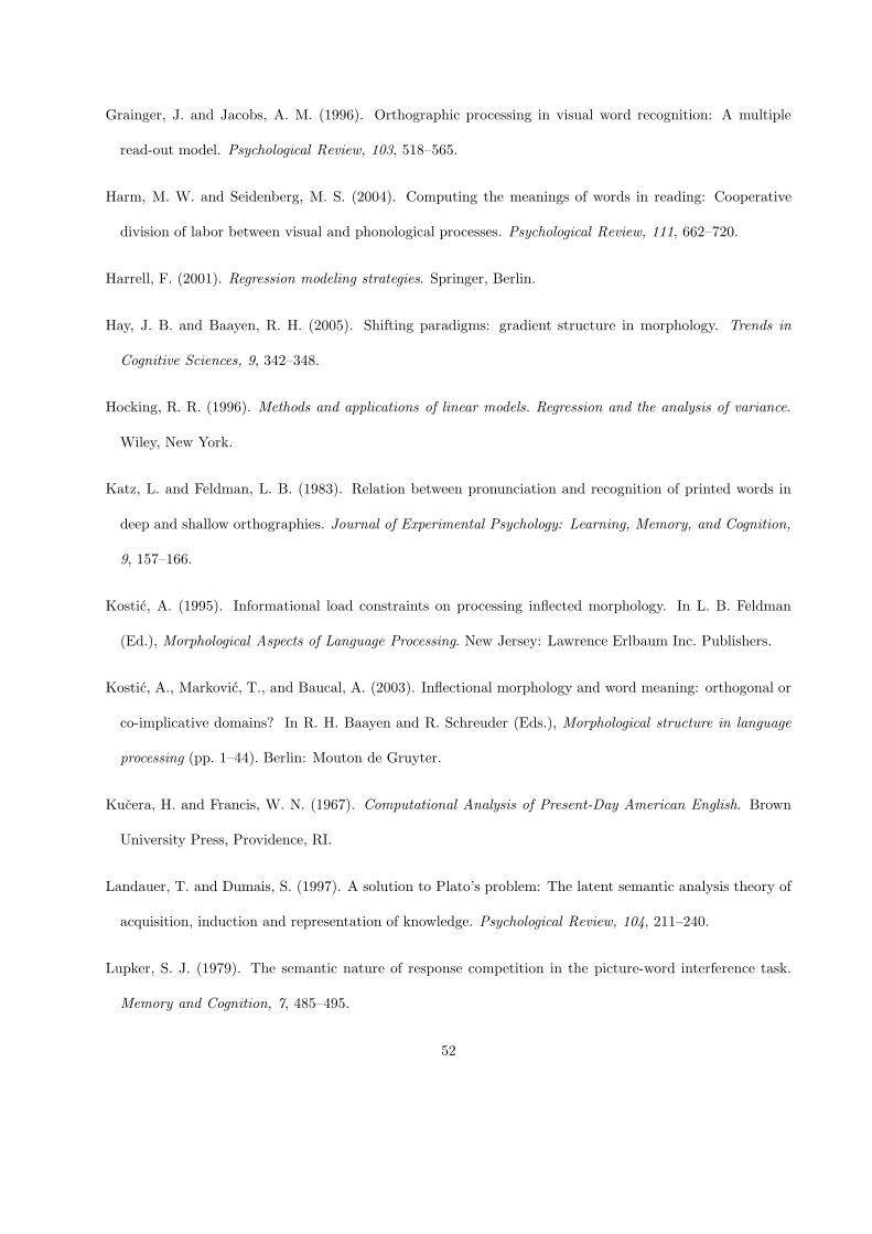
Grainger, J. and Jacobs, A. M. (1996). Orthographic processing in visual word recognition: A multiple
read-out model. Psychological Review, 103, 518–565.
Harm, M. W. and Seidenberg, M. S. (2004). Computing the meanings of words in reading: Cooperative
division of labor between visual and phonological processes. Psychological Review, 111, 662–720.
Harrell, F. (2001). Regression modeling strategies. Springer, Berlin.
Hay, J. B. and Baayen, R. H. (2005). Shifting paradigms: gradient structure in morphology. Trends in
Cognitive Sciences, 9, 342–348.
Hocking, R. R. (1996). Methods and applications of linear models. Regression and the analysis of variance.
Wiley, New York.
Katz, L. and Feldman, L. B. (1983). Relation between pronunciation and recognition of printed words in
deep and shallow orthographies. Journal of Experimental Psychology: Learning, Memory, and Cognition,
9, 157–166.
Kostic, A. (1995). Informational load constraints on processing inflected morphology. In L. B. Feldman
(Ed.), Morphological Aspects of Language Processing. New Jersey: Lawrence Erlbaum Inc. Publishers.
Kostic, A., Markovic, T., and Baucal, A. (2003). Inflectional morphology and word meaning: orthogonal or
co-implicative domains? In R. H. Baayen and R. Schreuder (Eds.), Morphological structure in language
processing (pp. 1–44). Berlin: Mouton de Gruyter.
Kucera, H. and Francis, W. N. (1967). Computational Analysis of Present-Day American English. Brown
University Press, Providence, RI.
Landauer, T. and Dumais, S. (1997). A solution to Plato’s problem: The latent semantic analysis theory of
acquisition, induction and representation of knowledge. Psychological Review, 104, 211–240.
Lupker, S. J. (1979). The semantic nature of response competition in the picture-word interference task.
Memory and Cognition, 7, 485–495.
52
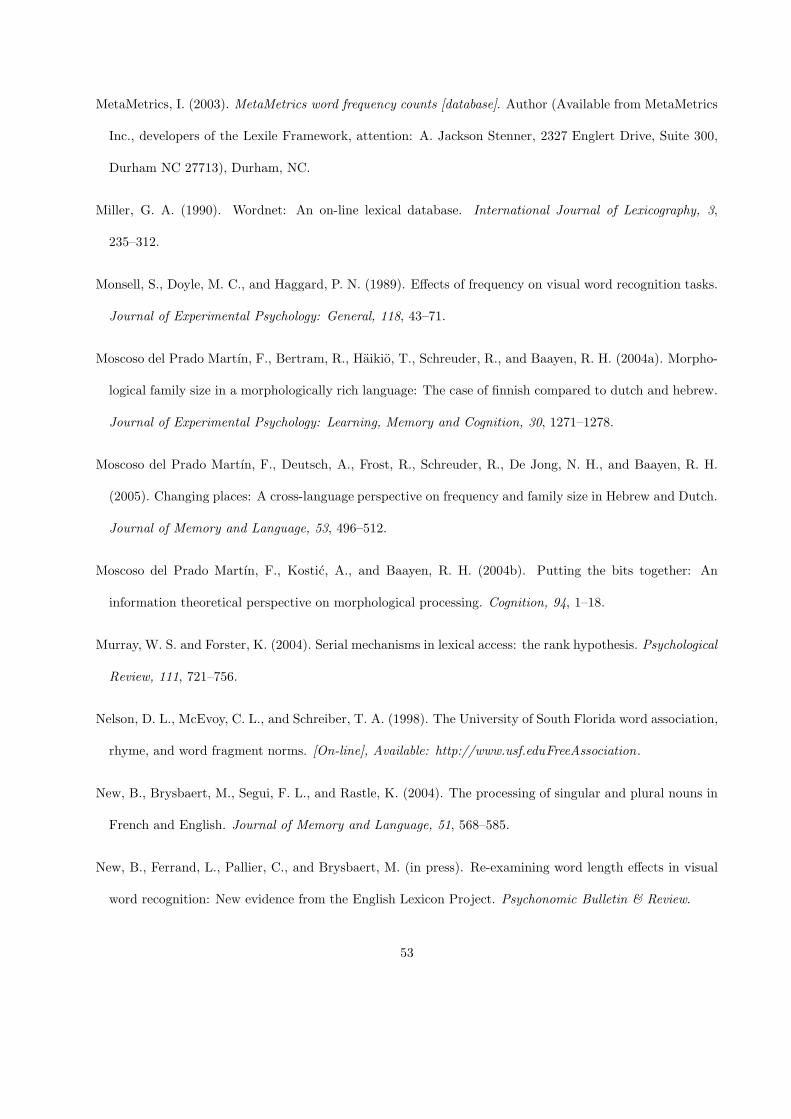
MetaMetrics, I. (2003). MetaMetrics word frequency counts [database]. Author (Available from MetaMetrics
Inc., developers of the Lexile Framework, attention: A. Jackson Stenner, 2327 Englert Drive, Suite 300,
Durham NC 27713), Durham, NC.
Miller, G. A. (1990). Wordnet: An on-line lexical database. International Journal of Lexicography, 3,
235–312.
Monsell, S., Doyle, M. C., and Haggard, P. N. (1989). Effects of frequency on visual word recognition tasks.
Journal of Experimental Psychology: General, 118, 43–71.
Moscoso del Prado Martın, F., Bertram, R., Haikio, T., Schreuder, R., and Baayen, R. H. (2004a). Morpho-
logical family size in a morphologically rich language: The case of finnish compared to dutch and hebrew.
Journal of Experimental Psychology: Learning, Memory and Cognition, 30, 1271–1278.
Moscoso del Prado Martın, F., Deutsch, A., Frost, R., Schreuder, R., De Jong, N. H., and Baayen, R. H.
(2005). Changing places: A cross-language perspective on frequency and family size in Hebrew and Dutch.
Journal of Memory and Language, 53, 496–512.
Moscoso del Prado Martın, F., Kostic, A., and Baayen, R. H. (2004b). Putting the bits together: An
information theoretical perspective on morphological processing. Cognition, 94, 1–18.
Murray, W. S. and Forster, K. (2004). Serial mechanisms in lexical access: the rank hypothesis. Psychological
Review, 111, 721–756.
Nelson, D. L., McEvoy, C. L., and Schreiber, T. A. (1998). The University of South Florida word association,
rhyme, and word fragment norms. [On-line], Available: http://www.usf.eduFreeAssociation.
New, B., Brysbaert, M., Segui, F. L., and Rastle, K. (2004). The processing of singular and plural nouns in
French and English. Journal of Memory and Language, 51, 568–585.
New, B., Ferrand, L., Pallier, C., and Brysbaert, M. (in press). Re-examining word length effects in visual
word recognition: New evidence from the English Lexicon Project. Psychonomic Bulletin & Review.
53
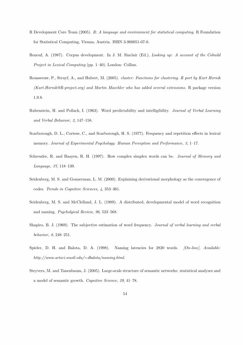
R Development Core Team (2005). R: A language and environment for statistical computing. R Foundation
for Statistical Computing, Vienna, Austria. ISBN 3-900051-07-0.
Renouf, A. (1987). Corpus development. In J. M. Sinclair (Ed.), Looking up: A account of the Cobuild
Project in Lexical Computing (pp. 1–40). London: Collins.
Rousseeuw, P., Struyf, A., and Hubert, M. (2005). cluster: Functions for clustering. R port by Kurt Hornik
([email protected]) and Martin Maechler who has added several extensions. R package version
1.9.8.
Rubenstein, H. and Pollack, I. (1963). Word predictability and intelligibility. Journal of Verbal Learning
and Verbal Behavior, 2, 147–158.
Scarborough, D. L., Cortese, C., and Scarborough, H. S. (1977). Frequency and repetition effects in lexical
memory. Journal of Experimental Psychology: Human Perception and Performance, 3, 1–17.
Schreuder, R. and Baayen, R. H. (1997). How complex simplex words can be. Journal of Memory and
Language, 37, 118–139.
Seidenberg, M. S. and Gonnerman, L. M. (2000). Explaining derivational morphology as the convergence of
codes. Trends in Cognitive Sciences, 4, 353–361.
Seidenberg, M. S. and McClelland, J. L. (1989). A distributed, developmental model of word recognition
and naming. Psycholgical Review, 96, 523–568.
Shapiro, B. J. (1969). The subjective estimation of word frequency. Journal of verbal learning and verbal
behavior, 8, 248–251.
Spieler, D. H. and Balota, D. A. (1998). Naming latencies for 2820 words. [On-line], Available:
http://www.artsci.wustl.edu/∼dbalota/naming.html.
Steyvers, M. and Tanenbaum, J. (2005). Large-scale structure of semantic networks: statistical analyses and
a model of semantic growth. Cognitive Science, 29, 41–78.
54
Tabak, W., Schreuder, R., and Baayen, R. H. (2005). Lexical statistics and lexical processing: semantic
density, information complexity, sex, and irregularity in dutch. In S. Kepser and M. Reis (Eds.), Linguistic
evidence — Empirical, Theoretical, and Computational Perspectives (pp. 529–555). Berlin: Mouton de
Gruyter.
Toglia, M. P. and Battig, W. (1978). Handbook of semantic word norms. Erlbaum, Hillsdale, NJ.
Traficante, D. and Burani, C. (2003). Visual processing of Italian verbs and adjectives: the role of the
inflectional family size. In R. H. Baayen and R. Schreuder (Eds.), Morphological structure in language
processing (pp. 45–64). Berlin; Mouton de Gruyter.
Venables, W. N. and Ripley, B. (2003). Modern applied statistics with R. Springer, New York.
Wood, S. N. (2006). Generalized additive models. An introduction with R. Chapman & Hall/CRC, New
York.
Zeno, S., Ivens, S., Millard, R., and Duvvuri, R. (1995). The educator’s word frequency guide. Touchstone
Applied Science, New York.
Zevin, J. and Seidenberg, M. (2002). Age of acquisition effects in word reading and other tasks. Journal of
Memory and Language, 47, 1–29.
55