15.053 February 8, 2007

More Linear and Non-linear Programming Models

including some non-linear optimization problems that can be made linear

plus applications to radiation therapy

1

Overview of Lecture

z Goals – get practice in recognizing and modeling linear

constraints and objectives – and non-linear objectives – to see a broader use of models in practice

2

3

Announcements

z Required “tutorials” on line. z Excel solver and help

– A goal: develop more Excel skills

Quotes for today

Reality is merely an illusion, albeit a very persistent one.

Albert Einstein

Everything should be made as simple as possible, but not one bit simpler.

Albert Einstein, (attributed)

“Reality is an illusion” is interesting in the context of 15.053. One wants to model “reality”, but all we can do is approximate reality. I could wax poetic on this philosophical theme, but won’t do so here.

We try to keep models as simple as possible. Too much detail in a model makes it extremely hard to get accurate information, and actually can lead to less accurate models in practice. One wants to capture the most important aspects of reality in a model, and not much more than that.

“Excel Tip of the Day” is a new feature this year. If you have any tips you want to share, please send them to me.

4

Overview

z Scheduling Postal Workers (5 in 7) – The model – Practical enhancements or modifications – Two non-linear objectives that can be made

linear

– A non-linear constraint that can be made linear

5

6

Scheduling Postal Workers z Each postal worker works for 5 consecutive days,

followed by 2 days off, repeated weekly.

Day Mon Tues Wed Thurs Fri Sat Sun

Demand 17 13 15 19 14 16 11

z Minimize the number of postal workers (for the time being, we will permit fractional workers on each day.)

I like this problem because it was one of the first scheduling problems that I saw as a graduate student, and it was the first one that I wrote a paper on. My paper, written in 1977, was of no lasting significance in and of itself and was never published. But it led me to an interest in optimization in which the requirements repeat periodically. I later wrote more than 10 papers on this topic as well as my Ph.D. dissertation.

Formulating as an LP

z Don’t look ahead.

z Let’s see if we can come up with what the decision variables should be.

z Discuss with your neighbor how one might formulate this problem as an LP.

7

8

The linear program

subject to x1 + x4 + x5 + x6 + x7 ≥ 17 Mon. x1 + x2 + x5 + x6 + x7 ≥ 13 Tues. x1 + x2 + x3 + x6 + x7 ≥ 15 Wed. x1 + x2 + x3 + x4 + x7 ≥ 19 Thurs. x1 + x2 + x3 + x4 + x5 ≥ 14 Fri.

x2 + x3 + x4 + x5 + x6 ≥ 16 Sat. x3 + x4 + x5 + x6 + x7 ≥ 11 Sun.

xj ≥ 0 for j = 1 to 7

Minimize z = x1 + x2 + x3 + x4 + x5 + x6 + x7

Day Mon Tues Wed Thurs Fri Sat Sun

Demand 17 13 15 19 14 16 11

This is a really unusual model in that the constraint of “5 days on followed by 2 days off” is handled by choosing the decision variables carefully. In particular, the first decision variable is the number of workers who start on Monday and work through Friday. The next 6 variables are chosen similarly. In this way, any selection of decision variables will automatically satisfy the constraint.

There are seven equality constraints, one for each day of the week. The first variable (the number of workers on the Monday to Friday shift) is part of each of the constraints on Monday through Friday. We normally view a linear program in terms of constraints and think of constraints one at a time. But sometimes it is useful to think of a variable and think of what the coefficients will be for that variable as we consider each constraint.

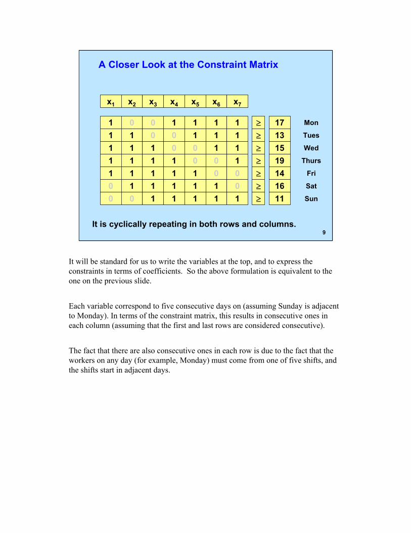
A Closer Look at the Constraint Matrix

x1 x2 x3 x4 x5 x6 x7

1 0 0 1 1 1 1 ≥ 17 1 1 0 0 1 1 1 ≥ 13 1 1 1 0 0 1 1 ≥ 15 1 1 1 1 0 0 1 ≥ 19 1 1 1 1 1 0 0 ≥ 14 0 1 1 1 1 1 0 ≥ 16 0 0 1 1 1 1 1 ≥ 11

Mon

Tues

Wed

Thurs

Fri

Sat

Sun

It is cyclically repeating in both rows and columns.

It will be standard for us to write the variables at the top, and to express the constraints in terms of coefficients. So the above formulation is equivalent to the one on the previous slide.

Each variable correspond to five consecutive days on (assuming Sunday is adjacent to Monday). In terms of the constraint matrix, this results in consecutive ones in each column (assuming that the first and last rows are considered consecutive).

The fact that there are also consecutive ones in each row is due to the fact that the workers on any day (for example, Monday) must come from one of five shifts, and the shifts start in adjacent days.

9

On the selection of decision variables

z A choice of decision variables that doesn’t work – Let yj be the number of workers on day j. – No. of Workers on day j is at least dj. (easy to formulate) – Each worker works 5 days on followed by 2 days off (hard).

z Conclusion: sometimes the decision variables incorporate constraints of the problem. – Hard to do this well, but worth keeping in mind – We will see more of this in integer programming.

10

It is natural to try to start with a decision variable corresponding to the number of workers on each day. Unfortunately, it would not be possible to add the constraint that each worker works for five consecutive days under this choice of variables. (It’s hard to prove that it isn’t possible to model it. But you can try for yourself and see that it can’t be done. By the way, if you think you can do it, the odds are that you are wrong.)

For most of the models in 15.053, the choice of the decision variables is more straightforward. But in practice, problems can come up with complex constraints that are extremely difficult to model as constraints but which can be handled through a clever choice of decision variables.

11

Some Modifications of the Model

z Suppose that there was a pay differential. The cost of workers who start work on day j is cj per worker.

z Suppose that one can hire part time workers (one day at a time), and that the cost of a part time worker on day j is pj.

What are the new decision variables? What are the changes to the model?

When one develops a decision model in practice, it is often best to start with a simple model that captures only a little of reality and then add in more realistic constraints in subsequent steps. If one tries to capture the whole model in one step, it is often too complex and too difficult to do.

In addition, we want to emphasize that there are a lot of constraints and costs that can be handled using linear programming.

12

subject to x1 + x4 + x5 + x6 + x7 ≥ 17 x1 + x2 + x5 + x6 + x7 ≥ 13 x1 + x2 + x3 + x6 + x7 ≥ 15 x1 + x2 + x3 + x4 + x7 ≥ 19 x1 + x2 + x3 + x4 + x5 ≥ 14

x2 + x3 + x4 + x5 + x6 ≥ 16 x3 + x4 + x5 + x6 + x7 ≥ 11

xj ≥ 0 for j = 1 to 7

Minimize z =

What are the new decision variables?

Another Enhancement z Suppose that the desirable number of workers on day j

is dj, but it is not required. Let sj be the “excess” number of workers day j. sj > 0 if there are more workers on day j than dj; otherwise sj ≤ 0.

z What is the minimum cost schedule, where the “cost” of having too many workers on day j is fj(sj), which is a non-linear function?

13

In practice, it is often difficult to tell the difference between constraints and goals. A manager may say that she needs 17 workers on Monday, but we know that the firm will function OK with 16, albeit perhaps not as well. So, it is not a “hard constraint”, and we may refer to it as a “soft constraint”, that is, one that can be violated. A hard constraint is one that can never be violated.

In this model, we treat the number of workers on each day as a goal for the day, and penalize not reaching the goal exactly. Having too many workers may be inefficient uses of labor. Having too few workers may make it difficult to handle the tasks for the day.

14

subject to x1 + x4 + x5 + x6 + x7 d1

x1 + x2 + x5 + x6 + x7 d2

x1 + x2 + x3 + x6 + x7 d3

x1 + x2 + x3 + x4 + x7 d4

x1 + x2 + x3 + x4 + x5 d5

x2 + x3 + x4 + x5 + x6 d6

x3 + x4 + x5 + x6 + x7 d7

xj ≥ 0 for j = 1 to 7

z =Minimize

What are the new decision variables?

What is the resulting non-linear model?

Often students will try to come up with something more complex than minimizing f1(s1) + … f7(s7). Once it is pointed out that this is the correct objective, students find it quite obvious.

On non-linear functions

z Occasionally a non-linear program can be transformed into a linear program.

z Rare, but useful when it occurs

z In general, non-linear programming solvers can work well on a minimization problem when the objective function is convex

15

Non-linear objectives occur very frequently in practice. In linear programming, we sometimes try to approximate non-linear functions using linear functions. This may lead to a significant loss of accuracy. If a linear approximation is very inaccurate, we can keep the non-linear objectives and use a non-linear programming solver. Unfortunately, it is much harder to solve a non-linear program than a linear program.

A great situation occurs when the non-linear program can be transformed into a linear program without any loss of accuracy. We will soon give a couple of examples of this very fortuitous situation.

Examples of Non-linear Functions

∑7 s j 2

j=1( ) sum of squared s’s

∑7 j

2

j=1 j ( ) weighted sum of squared s’sc s

∑7

j=1| sj | sum of absolute values of s’s

2∑7

j=1 x j −∑7

j=1 sj twice number of workers – sum of s’s

7 7 s s∑ ∑ i ji=1 j=1

An objective function is called separable if it can be expressed as the sum of functions of 1 variable.

16

There are a lot of nice modeling properties of the sum of squares, and it is a commonly used objective in practice. For example, in finance models, minimizing risk corresponds to minimizing variance, which can be expressed as a quadratic function.

It takes a lot longer to explain how minimizing risk in finance can sometimes be represented as a non-linear program, and so I will only provide this “teaser” here.

Separable non-linear objectives are often much easier to deal with, and such problems can typically be solved faster.

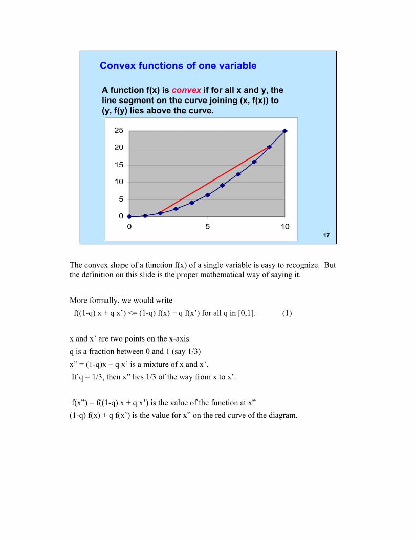
Convex functions of one variable

A function f(x) is convex if for all x and y, the line segment on the curve joining (x, f(x)) to (y, f(y) lies above the curve.

17

0

5

10

15

20

25

0 5 10

The convex shape of a function f(x) of a single variable is easy to recognize. But the definition on this slide is the proper mathematical way of saying it.

More formally, we would write f((1-q) x + q x’) <= (1-q) f(x) + q f(x’) for all q in [0,1]. (1)

x and x’ are two points on the x-axis. q is a fraction between 0 and 1 (say 1/3) x” = (1-q)x + q x’ is a mixture of x and x’. If q = 1/3, then x” lies 1/3 of the way from x to x’.

f(x”) = f((1-q) x + q x’) is the value of the function at x” (1-q) f(x) + q f(x’) is the value for x” on the red curve of the diagram.

18 NoYes NoYesYes

Which functions are convex?

f(x) = x2 f(x) = x3 for x ≥ 0 f(x) = x.5

f(x) = |x| Step Function whatever

Ye Nos No

If you guessed wrong for any of these curves, please review the definition of convexity.

19

The max of several linear functions is convex.

5 10

5

15

f1(x) = x/3

f2(x) = 3

f3(x) = 5 – x/2

f(x) = max{f1(x), f2(x), f3(x)}

The example gives the max of three linear functions of one variable. But a max of linear functions of more than one variable is also convex. In fact, the max of convex functions is convex.

We can see that the max of two convex functions is convex as follows:Suppose that f( ) and g( ) are both convex functions. Let h(x) = max(f(x), g(x)).We will show that h(x) is convex.Suppose that q ∈ [0, 1]. Let x” = (1-q) x + q x’

Then h(x”) = max {f(x”), g(x”)} <= max {(1-q) f(x) + q f(x’), (1-q) g(x) + q g(x’)}

<= (1-q) max {f(x), g(x)} + q max {f(x), g(x)} = (1-q) h(x) + q h(x’), showing that h(x) is convex.

On friendly** objective functions

z We will say that f(x) is a friendly non-linear function if it can be written as the max of one or more linear functions.

z We say that an objective function for a minimization problem is friendly if it is a friendly non-linear function or the sum of friendly non-linear functions.

z If a minimization problem P* has a friendly objective function its feasible region is that of an LP, then P* can be expressed as a linear program.

** “Friendly” is a term used in 15.053. Prof. Orlin made it up. 20

OK. “Friendly” may seem like a weird term, but mathematics is filled with such terms. And converting a non-linear program to a linear program is so fortuitous that we should in some way acknowledge our gratefulness.

Note that minimizing a friendly objective function subject to linear constraints leads to an LP. But this is not true for maximization. In fact, maximizing a friendly objective function subject to linear constraints creates a very difficult problem to solve. It is at least as hard as an integer programming problem, a topic discussed in detail later in this semester.

21

On minimizing friendly objective functions

Example 1. minimize z = max{f1(x), f2(x), f3(x)}

subject to 0 ≤ x ≤ 15

minimize z

subject to z ≥ x/3

z ≥ 3

z ≥ 5-x/2

0 ≤ x ≤ 15

z ≥ fi(x) for i = 1 to 3

f1(x) = x/3

f2(x) = 3

f3(x) = 5 – x/2 5

5 10 15

This example illustrates a minimax program of one variable. But the same transformation shows that minimizing any friendly objective function subject to linear constraints induces a linear program.

22

min z = max{f1(x), f2(x), f3(x)}

s.t a ≤ x ≤ b

LP

min z

s.t z ≥ fi(x) for i = 1, 2, 3

a ≤ x ≤ b

Theorem. If (z*, x*) is optimal for the LP, then it is also optimal for the minimax problem.

5

5 10 15

Minimax Problem

Proof. x* is feasible for the minimax problem. If z* < max{f1(x*), f2(x*), f3(x*)}, then (z*, x*) is infeasible.

If z* > max{f1(x*), f2(x*), f3(x*)}, then (z*, x*) is not optimal for the LP.x*

23

min z = max { fi(x): 1 ≤ i ≤ K } s.t x ∈ F

LP

min z

s.t z ≥ fi(x) for i = 1, …, K

x ∈ F Minimax Problem

Suppose that F is the set of feasible solutions for some linear programming problem.

Let x be a vector of decision variables.

Let fi(x) be a linear function in x for i = 1 to K.

Theorem. If (z*, x*) is optimal for the LP, then it is also optimal for the minimax problem.

We prove the theorem next.

Suppose that (z*, x*) is optimal for the LP. First one can show that x* is feasible for the minimax problem. This follows because x* ∈ F, and z* >= max {fi(x): 1 ≤ i ≤ K }. Now this doesn’t prove that z* = max {fi(x): 1 ≤ i ≤ K }. But if z* > max {fi(x): 1 ≤ i ≤ K }, then (z*, x*) is not optimal for the LP since one could replace z* by max {fi(x): 1 ≤ i ≤ K }, and get a lower objective. So, it follows that (z*, x*) is feasible for the minimax problem.

Now we show that there is no better LP solution. We do a proof by contradiction. Suppose that (z’, x’) were feasible for the minimax problem and z’ < z*. Then (z’, x’) would also be feasible for the linear program, contradicting that (z*, x*) is optimal for the LP. So, we conclude that (z*, x*) is optimal for the minimax problem.

Friendly objectives: Example 2 minimize the maximum number of excess workers needed on any day: that is

Minimize z = max {s1, …, s7}, where sj ≥ 0 for each j.

subject to x1 + x4 + x5 + x6 + x7 - s1 = 17 x1 + x2 + x5 + x6 + x7 - s2 = 13 x1 + x2 + x3 + x6 + x7 - s3 = 15 x1 + x2 + x3 + x4 + x7 - s4 = 19 x1 + x2 + x3 + x4 + x5 - s5 = 14

x2 + x3 + x4 + x5 + x6 - s6 = 16 x3 + x4 + x5 + x6 + x7 - s7 = 11

xj ≥ 0 , sj ≥ 0 for j = 1 to 7 24

Minimize z = max {s1, …, s7}, where sj ≥ 0 for each j.

We can express it as an LP as follows:

minimize subject to x1 + x4 + x5 + x6 + x7 - s1 = 17

x1 + x2 + x5 + x6 + x7 - s2 = 13 x1 + x2 + x3 + x6 + x7 - s3 = 15 x1 + x2 + x3 + x4 + x7 - s4 = 19 x1 + x2 + x3 + x4 + x5 - s5 = 14

x2 + x3 + x4 + x5 + x6 - s6 = 16 x3 + x4 + x5 + x6 + x7 - s7 = 11

xj ≥ 0 , sj ≥ 0 for j = 1 to 7

and also the constraints:

25

Friendly objectives: Example 3

Suppose the objective is minimize |s1| + … + |s7|. How do we modify it to make it linear?

Note: |sj| = max{sj, -sj} for each j.

The objective is the sum of friendly functions.

We do almost the same trick for minimizing the sum of friendly non-linear objective functions. But instead of creating one new variable z, we create a new variable zj for each term in the sum. so, the objective function becomes

Minimize z1 + z2 + … + z7

And we need to append the constraints z1 >= s1, z1 >= -s1

z2 >= s2, z2 >= -s2

…

z7 >= s7, z7 >= -s7

In any optimal solution, it will be true that zj = |sj| for j = 1 to 7.

26

27

subject to x1 + x4 + x5 + x6 + x7 d1

x1 + x2 + x5 + x6 + x7 d2

x1 + x2 + x3 + x6 + x7 d3

x1 + x2 + x3 + x4 + x7 d4

x1 + x2 + x3 + x4 + x5 d5

x2 + x3 + x4 + x5 + x6 d6

x3 + x4 + x5 + x6 + x7 d7

xj ≥ 0 for j = 1 to 7

Minimize

28

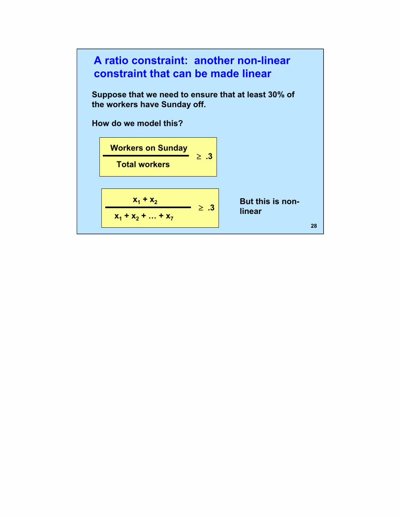
A ratio constraint: another non-linear constraint that can be made linear

Suppose that we need to ensure that at least 30% of the workers have Sunday off.

How do we model this?

Workers on Sunday

Total workers ≥ .3

x1 + x2

x1 + x2 + … + x7

≥ .3 But this is non-linear

29

Making it linear

Note: x1 + x2 + … + x7 > 0

Multiply both sides of the inequality by x1 + x2 + … + x7.

(x1 + x2 ) ≥ .3 (x1 + x2 + x3 + x4 + x5 + x6 + x7)

.7x1 + .7x2 - .3x3 - .3x4 - .3x5 - .3x6 - .3x7 ≥ 0

x1 + x2

x1 + x2 + … + x7

≥ .3

Note that this transformation assumes that the denominator x1 + … +x7 is strictly greater than 0. The non-linear constraint is not defined well if x1 + … + x7 = 0. In this particular problem, every feasible solution has x1 + … + x7 > 0, assuming that there is a demand for workers on some day. Thus, we don’t need worry about the issue of dividing 0 by 0.

Other enhancements

z Require that each shift has an integral number of workers – integer program

z Consider longer term scheduling

– model 6 weeks at a time

z Consider shorter term scheduling

– model lunch breaks

z Model individual workers

–permit worker preferences

30

This personnel scheduling problem illustrates a number of useful aspects of modeling. And it can go a long way towards useful modeling personnel scheduling problems in practice. Of course, in practical scheduling problems, one needs to address the problem at hand, whatever that problem may be.

Permitting a fractional number of workers is totally unrealistic, but the fractional solution of the model is usually easy to deal with in practice. Managers are often comfortable taking a fractional solution and rounding off the fractional parts. It often leads to a solution that is almost as good in terms of the objective function and still satisfies the constraints. However, it is better if one can solve the integer program. And occasionally fractional solutions can’t be rounded to a good integer solution.

Personnel scheduling typically deals with longer term scheduling than one week because these models permit one to be fairer to the workers. For example, in the model above, most workers never get a Friday or Saturday off. But in longer term models, one can ensure that each worker can get part or all of a weekend off.

Also, scheduling lunch breaks can be quite a challenge.

And in some scheduling problems, one can make workers happier by giving them days off that they request, such as to accommodate special days.

Most of these added complexities cannot be modeled easily using linear programming, and rely on integer programming, which we will discuss later in this subject.

31

Time for a mental break

Cartoons are by Sidney Harris http://www.sciencecartoonsplus.com/index.htm

Math Programming and Radiation Therapy

z An important application area for optimization

z Thanks to Rob Freund and Peng Sung for some of the following slides

This is one of my favorite applications of linear and non-linear programming, in large part because it is so important, and in part because it is a great application to medical technology.

32

Cancer cells

Normal cells

Figure by MIT OCW.

Math Programming and Radiation Therapy

z High doses of radiation (energy/unit mass) can kill cells and/or prevent them from growing and dividing – True for cancer cells and normal cells

z Radiation is attractive because the repair mechanisms for cancer cells is less efficient than for normal cells

This discussion applies to radiation therapy, where there is high energy radiation beamed at a patient. It does not apply to proton beam techniques, which have different physical properties than the usual radiation therapy.

33

34

Radiation Imaging z Recent improvements in

imaging – MRI – CT Scan – other

Imaging can reveal precise characteristics of tumors, and make radiation treatment possible. In addition, the imaging is critical for surgeries. It can also help monitor the progress of chemo-therapy.

Radiation Delivery

z Improvements of deliveryof radiation

z New field: tomotherapyIMRT

“Optimizing the Delivery ofRadiation Therapy to Cancer patients,” by Shepard, Ferris, Olivera, and Mackie, SIAMReview, Vol 41, pp 721-744, 1999.

The radiation therapy for brain tumors is delivered by a machine that can deliver large doses of radiation beamed from different angles into the brain.

35

36

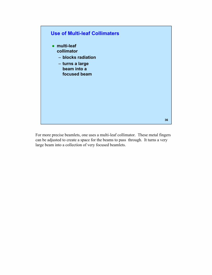
Use of Multi-leaf Collimaters

z multi-leaf collimator – blocks radiation – turns a large

beam into a focused beam

For more precise beamlets, one uses a multi-leaf collimator. These metal fingers can be adjusted to create a space for the beams to pass through. It turns a very large beam into a collection of very focused beamlets.

37

Conventional Radiotherapy

Relative Intensity of Dose Delivered

As radiation passes through the brain (or other parts of the body for other types of cancer), the radiation dose decreases as radiation is absorbed. The largest dose is where the beam enters the body. The smallest dose is where it leaves.

38

Conventional Radiotherapy

Relative Intensity of Dose Delivered

This very simple example shows the significance of aiming beams from multiple directions. Note that the largest dose is now in the center of the brain.

Conventional Radiotherapy

z In conventional radiotherapy – 3 to 7 beams of radiation – radiation oncologist and physicist work

together to determine a set of beam angles and beam intensities

– determined by manual “trial-and-error” process

39

The problem of determining optimal beamlets is absurdly difficult to solve by hand, especially when there are thousands of possible choices. Radiation oncologists are quite pleased to have optimization procedures help them out.

40

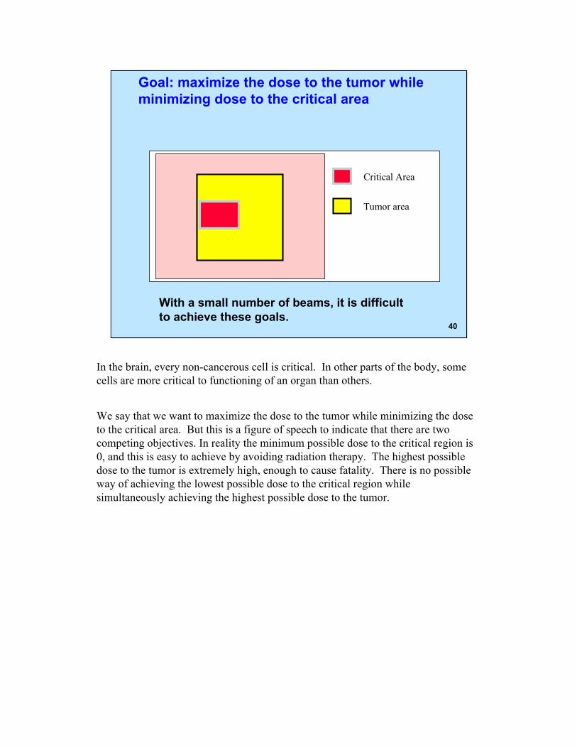
Goal: maximize the dose to the tumor while minimizing dose to the critical area

Critical Area

Tumor area

With a small number of beams, it is difficult to achieve these goals.

In the brain, every non-cancerous cell is critical. In other parts of the body, some cells are more critical to functioning of an organ than others.

We say that we want to maximize the dose to the tumor while minimizing the dose to the critical area. But this is a figure of speech to indicate that there are two competing objectives. In reality the minimum possible dose to the critical region is 0, and this is easy to achieve by avoiding radiation therapy. The highest possible dose to the tumor is extremely high, enough to cause fatality. There is no possible way of achieving the lowest possible dose to the critical region while simultaneously achieving the highest possible dose to the tumor.

Radiation Therapy: Problem Statement

z For a given tumor and given critical areas z For a given set of possible beamlet origins and

angles z Determine the weight of each beamlet such that:

– dosage over the tumor area will be at least a target level γL .

– dosage over the critical area will be at most a target level γU.

A natural way to try to balance the competing objectives is to put a lower limit on the amount of radiation delivered to the cancer cells and an upper limit on the amount of radiation delivered to critical cells. This is not the only way of trying to balance the competing objectives, as we shall see.

41

42

Display of radiation levels

Here is a nice picture of what can be achieved using linear programming. The orange and red regions indicate the parts of the figure with the highest radiation levels.

43

Linear Programming Model

z First, discretize the space – Divide up region into a 2D (or 3D) grid of pixels

To model this problem using linear programming, the decision variables will correspond to how much radiation is delivered from each possible beamlet.

In order to determine whether a cell gets too much or too little radiation, we aggregate the cells into “pixels.” If we didn’t divide up the region into pixels, we could end up with one constraint for each neuron, leading to 100s of billions of constraints.

More on the LP

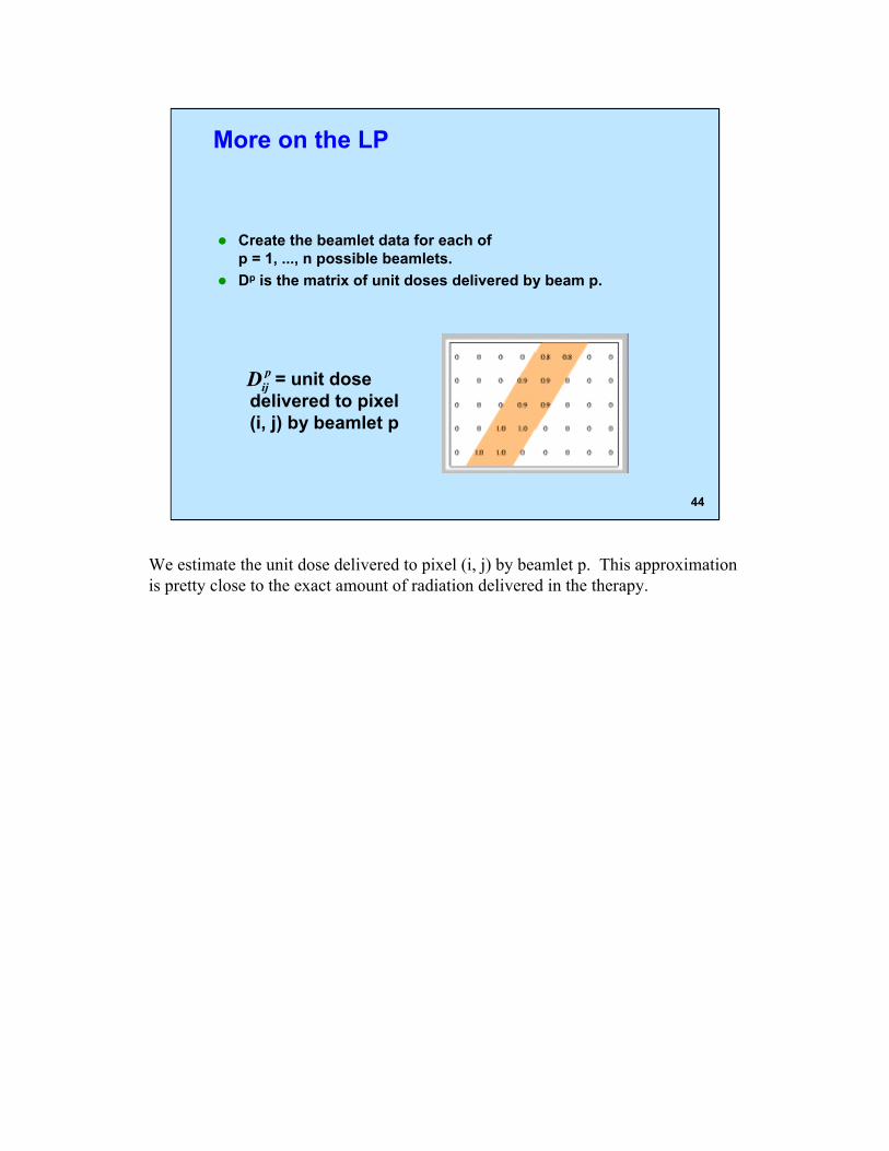
z Create the beamlet data for each of p = 1, ..., n possible beamlets.

z Dp is the matrix of unit doses delivered by beam p.

Dipj = unit dose

delivered to pixel (i, j) by beamlet p

44

We estimate the unit dose delivered to pixel (i, j) by beamlet p. This approximation is pretty close to the exact amount of radiation delivered in the therapy.

45

Linear Program

z Decision variables w = (w1, ..., wp) z wp = intensity weight assigned to beamlet p

for p = 1 to n;

z Dij = dosage delivered to pixel (i, j)

1== ∑n p

ij ij pp D D w

The primary place where linear programming equality constraints are used is here. The total dosage delivered to a pixel is the sum of the doses delivered by all the beamlets to that pixel.

An LP model

took 4 minutes to

minimize ∑ ( , ) D solve in 1999.

i j ij

pD =∑n

p=1 D w ij ij p

Dij ≥ γ L for ( , i j )∈T

Dij ≤ γ U for ( , i j )∈C

wp ≥ 0 for all p

In an example reported in the paper, there were more than 63,000 variables, and more than 94,000 constraints (excluding upper/lower bounds)

This linear program is pretty simple conceptually. It says that we need a sufficiently large dose at tumor cells and a sufficiently small dose at critical areas.

46

∑ ( , ) iji jD

γ≥ ∈ for ( , )ij LD i j T

γ≤ ∈ for ( , )ij UD i j C

47

What happens if the model is infeasible?

1== ∑n p

ij ij pp D D w

minimize

0≥ for all pw p

γ+ ≥ ∈ for ( , )ij ij LD y i j T

∑ ( , ) iji j y

0≥ for all ( , )ijy i j

Allow the constraint for pixil (i,j) to be violated by an amount yij, and then minimize the violations.

γ− ≤ ∈ for ( , )ij ij UD y i j C

A doctor will naturally try to set the threshold for cancer cells as high as he or she can achieve while setting the threshold for critical cells as low as possible. Even with lots of experience in what is achievable, there is a natural tendency for the doctor to set these parameters so that there is no feasible solution. In this case, then the doctor would keep adjusting the parameters until eventually getting a feasible solution. This can be a time consuming process.

∑ ( , ) iji jD

γ≥ ∈ for ( , )ij LD i j T

γ≤ ∈ for ( , )ij UD i j C

∑ ( , ) iji jy

48

An even better model

1== ∑n p

ij ij pp D D w

minimize

0≥ for all pw p

γ+ ≥ ∈ for ( , )ij ij LD y i j T

0≥ for all ( , )ijy i j

minimize the sum of squared violations.

γ− ≤ ∈ for ( , )ij ij UD y i j C

( )2

∑ ( , ) iji j y

This is a nonlinear program (NLP). This one can be solved efficiently.

Least squares

It is far easier to set the parameters conservatively (as far as the patient is concerned) while allowing some violation. If there is no feasible solution to the problem on the previous slide, there will definitely be a feasible solution to this non-linear program since one can choose yij to guarantee feasibility.

The objective function would try to set all of the y’s to 0. Failing that, it would set all of the y’s as small as possible.

The quadratic function is used instead of a linear function in recognition that it is better to have a slightly higher dose for a large number of critical cells than an incredibly high dose for a lesser number of cells. The latter situation would result in killing more critical cells.

Similarly, we don’t want to miss cancer cells with the radiation because those cells would be the most likely to grow and create more cancer. So, we would prefer a slightly lower dose for a large number of cancer cells than having a much lower dose for some cancer cells.

49

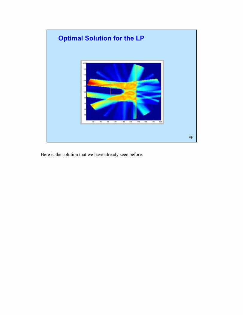
Optimal Solution for the LP

Here is the solution that we have already seen before.

50

An Optimal Solution to an NLP

The NLP worked much better. I suspect that this is true in general, but one example is not enough to prove it.

Is that the end of the story on modeling?

z Other issues: – Delivering the radiation doses quicker by

setting the multi-leaf collimators optimally. – trying to keep average radiation levels low

over part of the critical region. – how do we trade off the doses to the critical

area with doses to the tumor?

51

The doctors are very excited about using optimization to set beams. But it still opens lots of other questions. If the optimization can set the multi-leaf collimators optimally, then we can speed up the delivery of the radiation, and this permits more patients to use the machine. Optimizing the use of the multi-leaf collimators is a challenging problem, often relying on results in network optimization.

Also doctors are concerned with radiation delivery over larger areas than single cells, and want solutions that keep average radiation levels low over the critical region. If these constraints are modeled in a straightforward manner, it leads to problems that are extremely hard to solve.

There is often a balance in practice of figuring out the right level of fidelity needed for a model. Too much fidelity may make the model too hard to solve, and often too hard to validate. Tool little fidelity can mean that we are solving a model that is too different from reality to be of much use.