Monsoon dynamics with interactive forcing, Part I:

Axisymmetric studies

Nikki C. Prive∗and R. Alan Plumb

Program in Atmospheres, Oceans, and Climate,

Massachusetts Institute of Technology, Cambridge, Massachusetts

∗Corresponding author address: N. Prive, NOAA/ESRL, R/GSD, 325 Broadway Boulder, CO 80305-3337. email: nprive@alum.mit.edu

Abstract

The applicability of axisymmetric theory of angular momentum conserving circula-

tions to the large-scale steady monsoon is studied in a general circulation model with

idealized representations of continental geometry and simple physics. Results from an

aquaplanet setup with localized subtropical forcing are compared with a continental

case. It is found that the meridional circulation which develops is close to angular mo-

mentum conserving for cross-equatorial circulation cells, both in the aquaplanet and

in the continental cases. The equator proves to be a substantial barrier to boundary

layer meridional flow; flow into the summer hemisphere from the winter hemisphere

tends to occur in the free troposphere rather than in the boundary layer. A theory is

proposed to explain the location of the monsoon; assuming quasi-equilibrium, the pole-

ward boundary of the monsoon circulation is colocated with the maximum in subcloud

moist static energy, with the monsoon rains occurring near and slightly equatorward

of this maximum. The model results support this theory of monsoon location, and it

is found that the subcloud moist static energy distribution is determined by a balance

between surface forcing and advection by the large scale flow.

1

1. Introduction

The classic view of the monsoon has been founded on the existence of a strong contrast in

heating between the ocean and land, with the monsoon itself manifesting as an enormous

sea-breeze (Halley, 1686). However, this depiction of monsoon dynamics fails to account

for some of the observed behaviors of the monsoon, including abrupt delayed onset and the

active-break cycle, and does not consider the impact of planetary rotation on such a large-

scale flow. An alternative view which considers the monsoon as a seasonal displacement of

the intertropical convergence zone (ITCZ) into the subtropics has recently gained support

(eg. Chao and Chen (2001), Gadgil (2003)). It is this latter view which is the focus of this

work.

The observed zonally averaged monsoon flow (not shown) depicts a global meridional

circulation cell with ascent in the monsoon region, outflow which crosses into the winter

hemisphere aloft, subsidence in the winter hemisphere tropics, and cross-equatorial return

flow at low levels. Using a linear shallow-water model, Gill (1980) found that a localized

prescribed forcing in the off-equatorial tropics induces a cross-equatorial circulation similar

to the observed monsoon flow. However, Held and Hou (1980), Lindzen and Hou (1988),

and Plumb and Hou (1992) determined the axisymmetric Hadley circulation to be funda-

mentally nonlinear, and predicated upon the conservation of angular momentum in the free

troposphere. The intent of this work is explore the validity of the nonlinear, axisymmetric

theory of the steady Hadley circulation in describing the dynamics of the monsoon.

Held and Hou (1980) expanded upon the work of Hide (1969) and Schneider (1977) to

explain the development of the annual mean Hadley cells using concepts of angular momen-

tum conservation. The predominance of a single Hadley cell in the dynamical response to

solsticial forcing was examined by Lindzen and Hou (1988). Plumb and Hou (1992) explored

the atmospheric response to a localized subtropical forcing in a dry, axisymmetric framework

and found that the critical condition for the development of an angular momentum conserv-

ing (AMC) meridional circulation is the existence of an extremum of angular momentum

2

in the thermal equilibrium state. Emanuel (1995) showed that assuming a moist adiabatic

lapse rate, and making use of the Maxwell relations, the threshold may be written as

[

∂

∂φ

(

cos3φ

sinφ(Ts − Tt)

∂sb

∂φ

)]

= −4Ω2a2cos3φ sinφ (1)

where φ is the latitude, a is the radius of the earth, Ω is the angular velocity of the earth, sb

is the subcloud moist entropy, Ts is the surface temperature, and Tt is the temperature at the

tropopause. Zheng (1998) verified threshold behavior in a moist axisymmetric aquaplanet

model with fixed, local subtropical SST perturbation.

There has been interest in the application of the theory of threshold behavior to explain

certain aspects of the monsoon. Plumb and Hou hypothesized that the abrupt onset of the

monsoon might be related to this threshold behavior. Eltahir and Gong (1996) found that

the subtropical meridional gradient of subcloud moist entropy was positively correlated with

the strength of the West African monsoon.

There are several limitations to the existing nonlinear theory of the Hadley circulation.

First, the work of Held and Hou (1980), Lindzen and Hou (1988), and Plumb and Hou (1992)

is in a dry framework with an assigned distribution of radiative equilibrium temperature. In

these cases, the induced circulation does not affect the forcing field, while in the real world,

the forcing is highly dependent upon the circulation. For the moist experiments of Emanuel

(1995) and Zheng (1998), a prescribed SST perturbation was used to force the atmosphere,

with radiative convective equilibrium temperatures following a moist adiabat to communi-

cate the surface forcing throughout the troposphere. Over a dry landmass forced by surface

fluxes, the vertical column follows close to a dry adiabat, and upper level temperatures may

be relatively cold even though the lower tropospheric temperatures are high. This raises the

question of whether strong sensible heat fluxes over an arid continent are sufficient to induce

a monsoonal circulation. Also, given the interaction possible between the circulation and

the forcing, the location and extent of the monsoon are not predictable from the radiative

convective equilibrium state.

3

A second limitation is that the nonlinear theory is concerned with the steady state

circulation, rather than the transient monsoon. The timescale for circulations to reach a

steady state in axisymmetric models is frequently quite long, on the order of hundreds of

days, which is much greater than the seasonal timescale associated with monsoons. Fang

and Tung (1999) found that the abrupt increase in circulation strength observed when the

steady forcing is shifted off of the equator was not seen when transient forcing was used.

In addition to the theory and models of the Hadley circulation, axisymmetry has been ap-

plied specifically to monsoon circulations, such as the work of Webster (1983) and Goswami

and Shukla (1984). These two studies focused on the intraseasonal variability of the mon-

soon, and showed that interaction between the dynamics of the monsoon flow and surface

heat fluxes significantly contributes to the transient behavior of the monsoon. We wish

to take a similar approach as these seminal papers, but with a focus on the steady-state

monsoon.

In order to address the applicability of the nonlinear axisymmetric theory of Hadley

circulations to the interactive monsoon, we wish to address the following questions:

1. How does the presence of a subtropical continent with interactive forcing affect the

monsoon circulation?

2. What determines the location and extent of the monsoon?

3. Is the steady monsoon circulation representative of the dynamics of the transient

monsoon?

An axisymmetric general circulation model is used to explore these questions.

This paper focuses on axisymmetric modelling as a first step towards developing an

understanding of the large-scale monsoon circulation. The observed monsoon is strongly

asymmetric, so that the applicability of a strict axisymmetric theory is questionable. The

question of asymmetry of the flow will be addressed in a companion paper; the current work

seeks to address only the purely axisymmetric case.

4

There is a wide gap in modeling the monsoon between the highly idealized axisymmetric

theory and full GCM studies with realistic physics. While the axisymmetric theory is useful

for developing an understanding of the basic physical mechanisms which drive and affect

the monsoon, it is unclear how the simplifications which are involved limit the applicability

to the monsoon. On the other hand, the wealth of feedbacks present in the full GCM

studies make diagnosis of the monsoon behavior extremely difficult. The goal of this work

is to bridge the gap between the idealized axisymmetric theory and the more complex,

interactive monsoon. A general circulation model with simplified representations of some

physical processes and with idealized continental geometry is chosen to achieve intermediate

complexity, as described in Section 2. This allows for a reasonably more realistic portrayal

of processes which are suspected to be intrinsic to the monsoon, while at the same time

reducing the feedbacks to make analysis more tractable.

The first step is to characterize the Hadley response to a steady local subtropical forcing

in an aquaplanet setup. The aquaplanet cases act as a basis of comparison for the later,

more complex, cases with a subtropical continent. The subtropical forcing takes the form of

an SST perturbation, the form of which is designed to mimic the presence of a landmass in

order to allow direct comparison with continental experiments. The results of the aquaplanet

cases are described in Section 3, where it is found that threshold behavior of the meridional

circulation is seen as predicted by Plumb and Hou (1992) and Emanuel (1995). It is found

that the strength of the circulation weakens as the forcing is shifted poleward.

Next, a simple subtropical continent is introduced with perpetual summer forcing, and

comparison with the aquaplanet experiments helps to determine the impact of continental

physics on the monsoon circulation. These experiments are discussed in Section 4. Threshold

behavior of the circulation strength is not observed as clearly as in the aquaplanet cases,

although the circulation does show a transition from local to global extent, as predicted by

the nonlinear theory. A theory of monsoon location is introduced in Section 5. The boundary

layer thermodynamics are shown to control the extent and location of the monsoon region

5

such that the zero line of the circulation must be coincident with the maximum in subcloud

moist static energy. Over the ocean, the moist static energy is closely related to the surface

temperature, while over a land surface, the moist static energy is controlled by a balance

between advection by the large-scale flow and surface heat fluxes.

Finally, seasonally varying forcing is implemented over the landmass to contrast with the

perpetual summer cases to explore the applicability of the steady solutions to the transient

monsoon. Section 6 addresses these experiments. The transient response approaches the

perpetual summer circulation by mid to late summer, but the early summer state is not

close to the steady result. The timescale for the transient response is that needed for the

large-scale overturning circulation to fold over the contours of angular momentum across

the tropical upper troposphere. The overall findings are discussed in Section 7.

2. Model

The model used is the MIT General Circulation Model (MITGCM), release 1.0. The MIT-

GCM consists of a dynamical core coupled to an atmospheric physics package; the dynamical

kernel of the model is described by Marshall et al. (2004). The atmospheric MITGCM has

been tested extensively against Held and Suarez (1994), although a different atmospheric

physics package is implemented here. The model gridspace used is a partial sphere between

64S and 64N , with 40 pressure levels in the vertical at 25 mb intervals. A staggered

spherical polar grid is used with 4 latitudinal resolution. There is no orography, and the

surface is assigned to the 1012.5 mb pressure level. The coefficient of vertical viscosity is

10 Pa2/s, and an eighth-order Shapiro filter is employed to reduce horizontal noise in the

temperature, humidity, and horizontal flow fields.

Radiation and cloud physics are not included; instead, the atmosphere undergoes New-

tonian cooling:

QNC = τ−1

NC(TNC − T ) (2)

6

where T is the temperature at a gridpoint, and QNC is the cooling rate. The timescale for

cooling, τNC , is chosen to be 60 days; the qualitative behavior of the circulation was found

to be similar over a range of τNC . TNC = 200 K for all gridpoints; this profile for TNC is

chosen for its simplicity in keeping with the idealized nature of the model setup.

The moist convective scheme of Emanuel (1991) is used, including the modifications of

Emanuel and Zivkovic-Rothman (1999). The convective parameters used as part of this

scheme have been optimized against observed data from the Tropical Ocean Global Atmo-

sphere Coupled Ocean-Atmosphere Response Experiment (Emanuel and Zivkovic-Rothman,

1999). The convection scheme includes dry adiabatic adjustment, which is performed over

regions which are unstable to unsaturated ascent. A mixed layer of momentum is included

at the lowest 200 mb of the model; in this layer, horizontal velocities are homogenized over

a timescale of 500 sec.

Very simple representations of ocean and land surfaces are implemented. SSTs are

prescribed over the ocean, with temperature profile fixed in time. Over land, a bucket

hydrology following Manabe (1969) is used. Surface evaporation is modified by a factor B

B =

1 B ≥ 0.75B0

B0.75B0

B < 0.75B0

(3)

∂B

∂t= P − E

where B0 is an assigned bucket depth (20 cm) indicating the amount of moisture that can

be stored per unit surface area, B is the current moisture in the bucket per unit area, E

is the evaporation rate, and P is the precipitation rate. Any excess moisture gained by

precipitation is considered to be runoff. The initial moisture content of the buckets for each

model case was assigned to be zero.

Because a Newtonian cooling scheme is used, the flux balance at the surface cannot be

calculated using radiative fluxes. Instead, the net downward flux into the surface (THF) is

7

prescribed as a function of latitude:

THF (φ) = LHF (Ts) + SHF (Ts) (4)

where φ is the latitude, LHF is the latent heat flux into the atmosphere, SHF is the sensible

heat flux into the atmosphere, and Ts is the surface temperature. The surface temperature

and heat fluxes are interdependent and calculated iteratively. Using a prescribed net ra-

diative flux has the benefits of allowing direct control over the land surface forcing and of

reducing the number of feedbacks, such as cloud-radiative feedbacks, in comparison to a sit-

uation with interactive radiation. This permits easier diagnosis of the underlying dynamical

mechanisms, but at the cost of making the resulting flow less realistic. For example, surface

temperatures may become very hot over a desert-like land area as there no increase in the

outgoing longwave radiation with increased surface temperatures. Direct control of the land

surface forcing allows the behavior of the monsoon to be explored in parameter space by

testing a range of forcing strengths.

3. Aquaplanet

The response of the atmosphere to a localized subtropical forcing is examined in an aqua-

planet setup. These cases will form a baseline for comparison with the continental cases.

The model is spun up from rest with SST of 302K at all latitudes for 200 days, then an SST

perturbation of the form

SST (φ) = 302K + ∆Tcos2(5

2(φ − φ0)), φ0 < φ < (φ0 + 36) (5)

SST (φ) = 302K φ ≤ φ0, (φ0 + 36) ≤ φ

is introduced, where ∆T is the strength of the SST perturbation, and φ0 is the location of

the SST perturbation (Figure 1). The model is then integrated until an equilibrium state

8

is reached, typically 300-1000 days. This form of the local SST perturbation is chosen to

emulate the presence of a continent, with an abrupt interface between land and ocean in the

subtropics at φ0. The uniformly warm ocean temperature profile in the equatorial region

and southern hemisphere is chosen to isolate the atmospheric response to the local SST

perturbation. A range of ∆T are tested to characterize any threshold behavior.

a. Subtropical Threshold Behavior

Two criteria are used to determine whether the modeled Hadley circulations are in agreement

with the nonlinear theory: 1) conservation of angular momentum across the upper branch of

the circulation cell; 2) existence of threshold behavior of the circulation strength as described

by Plumb and Hou (1992) and Emanuel (1995). The ocean forcing is located at φ0 = 16N

(5); this latitude is chosen as representative of a subtropical monsoon. The strength of the

applied SST perturbation (∆T in (5)) is varied from 0.5 K to 2.5 K.

Threshold behavior of the circulation strength is clearly observed with critical ∆T =

1.25 K (Figure 2). When the SST perturbation is small, the resulting circulation is weak,

and the upper tropospheric absolute vorticity does not approach the critical value at zero.

Above the threshold forcing, the circulation intensifies much more rapidly with increased

∆T , and the upper level absolute vorticity is close to zero. When forcing levels are below

the threshold, the circulation is confined to one hemisphere and does not cross the equa-

tor (Figure 3). Above the threshold forcing, the circulation becomes cross-equatorial and

considerably stronger (Figure 3). In these cases, the upper tropospheric absolute vorticity

is close to zero in the circulation cell (Figure 2), which indicates conservation of angular

momentum.

9

b. Cross-Equatorial Flow

There is a tendency for cross-equatorial circulations to ‘jump’ in the lower troposphere when

approaching the equator (eg. Figure 3). While some of the flow crosses the equator in the

free troposphere, a portion of the circulation is confined to the southern hemisphere, giving

the streamfunction the appearance of two conjoined Hadley cells. This flow pattern results

in a secondary precipitation maximum (not shown) in the southern hemisphere tropics be-

tween the equator and 6S. The moisture content of the low-level flow is depleted during

the jump as the air rises to the mid-troposphere, but is replenished through large latent heat

fluxes at the surface in the northern hemisphere. Jumping also alters the streamfunction in-

tensity. When jumping does not occur, the maximum streamfunction of the cross-equatorial

circulation is located in the lower troposphere near the equator. The initiation of jumping

eliminates the lower tropospheric streamfunction maximum, and the circulation maximum

occurs in the upper troposphere. Double ITCZs are more common in atmospheric mod-

els than in the observed atmosphere (Zhang, 2001); however, the secondary precipitation

maximum seen in the present model results is not considered to be a doubled ITCZ.

Jumping of the meridional circulation has been addressed extensively by Pauluis (2001);

a brief synopsis is given here. A pressure gradient across the equator is needed in the mixed

layer in order to allow cross-equatorial flow. When the mixed layer is thin or the pressure

gradient is weak, only a limited mass flux is possible in the mixed layer, so flow attempting to

cross the equator must rise into the free troposphere in order to cross. In a moist atmosphere,

the vertical moist stability near the equator is weak, and the resulting jump is quite deep.

In the modeled case with uniform ocean SSTs, the pressure gradient across the equator is

very weak, sometimes even increasing northward, so that cross-equatorial flow is strongly

inhibited even though the mixed layer is quite deep. An example of an aquaplanet case in

which the flow does not jump at the equator is seen in the bottom left panel of Figure 4,

where the SST has a maximum at 8N and a southward-decreasing SST gradient across the

equator.

10

c. Latitudinal Influence on Circulation

A series of aquaplanet experiments are made with uniform SST and a localized boreal

hemisphere SST perturbation, which is varied in location. The form of the perturbation

is given by (5), with φ0 varied from 0N to 26N , and ∆T is chosen to be 4.25 K. This

high value of ∆T was chosen to yield cross-equatorial circulations for the entire range of φ0

tested.

The impact of the location of the forcing on the strength of the circulation is illustrated

in Figure 5. The maximum streamfunction increases as φ0 is moved poleward from 0N

to 6N , although the circulation width only broadens slightly (not shown), with no sign of

jumping behavior. These results are in accord with the findings of Lindzen and Hou (1988),

who showed that the Hadley circulation strengthens as the peak forcing is moved poleward

in the near equatorial region. As φ0 moves from 6N to 10N , the circulation nearly doubles

in width (not shown) but decreases sharply in strength as jumping initiates and the lower

tropospheric streamfunction maximum is destroyed. As φ0 is moved poleward from 10N

to 22N , the circulation decreases in strength and broadens slightly. As the circulation

broadens, the easterly jet intensifies significantly, resulting in greater viscous effects with

weakening angular momentum conservation in the upper branch of the circulation. This

increased viscosity, peculiar to numerical models, is hypothesized to account for the gradual

weakening of the circulation as the forcing is shifted poleward. The φ0 = 24N case is close

to the local-to-global AMC transition as described by Schneider (1983), but far above the

critical threshold for the existence of an AMC circulation (Plumb and Hou, 1992). Schneider

showed that an angular momentum conserving circulation forced by a δ-function source

undergoes a transition from a cell of regional extent to a cross-equatorial cell as the forcing

is increased; the transition forcing needed is greater when the forcing is moved poleward.

The proximity to this transition is the likely cause of the sharp reduction in streamfunction

magnitude from φ0 = 22N to 24N . With a weaker ∆T , the transition to a local circulation

occurs with φ0 closer to the equator.

11

4. Continental Cases

A subtropical continent with interactive surface temperatures and heat fluxes is introduced.

By comparing the results of these experiments with the results from the aquaplanet cases,

the peculiar nature of continental forcing of the large-scale circulation can be discerned. The

strength of the land surface forcing may be directly manipulated through the total surface

heat flux (4), given by

THF (φ) = THF0 − ∆THFsin2((φ − 8N)) (6)

where ∆THF is 50 W/m2, and THF0 ranges from 120 to 150 W/m2. This forcing profile was

chosen to represent a summer-mean forcing rather than a solsticial forcing. For all of these

cases, the continent extends from the southern coastline at 16N poleward to the model

boundary at 64N . For each case, the model is first spun up from rest for 200 days with a

relatively cold continent (THF0 = 80 W/m2). The land surface forcing is then increased to

the summer value over a period of 100 days, and the model is run for at least 700 additional

days until a steady state is reached.

a. Uniform SST

First, a series of experiments are performed wherein the ocean is assigned uniform tempera-

ture. The only difference between this case and the previous aquaplanet case with localized

SST perturbation at 16N is the replacement of the prescribed SST perturbation with an

interactive continent in the boreal hemisphere.

For the weakest continental forcing tested, THF0 = 120 W/m2, no monsoon occurs and

there is little precipitation over the continent (not shown). The meridional circulation is

limited to a very weak, shallow circulation just along the coastline, with subsidence in the

mid and upper troposphere over the continental subtropics.

When the land forcing is increased to 125 ≤ THF0 ≤ 130 W/m2, deep moist convection

12

onsets over the subtropical continent. Large scale ascent occurs along the coastline, with a

latitudinally narrow meridional circulation with subsidence over the tropical ocean (Figure

4). The upper tropospheric absolute vorticity (dotted line with squares, Figure 6) is not

close to the critical value at zero, and the deep circulation is not strongly angular momentum

conserving.

For land forcing of THF0 ≥ 135W/m2, the meridional circulation is more global in ex-

tent, with ascent over the subtropical continent and subsidence over the southern hemisphere

ocean (Figure 4). Jumping of the circulation occurs for all cases with cross-equatorial flow,

and becomes more pronounced as the land surface forcing increases. The upper level tropical

easterly jet (not shown) is very strong, which is a common feature in axisymmetric mod-

els. The angular momentum field (not shown) is significantly distorted by the circulation,

although the flow is able to cross some contours of angular momentum in the tropics, where

there is strong easterly shear. As the land forcing is increased, the circulation broadens and

the monsoon region moves inland, as shown in Figure 7.

Although the strength of the meridional circulation increases systematically with in-

creased land surface forcing (dotted line with squares in Figure 6), there is little indication

of threshold behavior. The upper level absolute vorticity (Figure 6) gradually approaches

the critical value at zero for THF0 ≥ 140W/m2, but a cross-equatorial circulation develops

when the vorticity is still sub-critical (THF0 = 135W/m2). The threshold behavior (Figure

6) may be compared with that of the aquaplanet case in Figure 2.

b. ’Summer’ SST

The experiments with uniform SSTs help to isolate the atmospheric response to a subtrop-

ical landmass, but the ocean forcing is far from realistic. A summer-like SST profile is

implemented with subtropical continent in an effort to achieve more realistic flow in the

13

equatorial region. The SST distribution is fixed and does not vary with time:

SST (φ) = SST0 − ∆Tsin2(φ − 8N) (7)

where SST0 = 302 K and ∆T = 28 K.

First, an aquaplanet case with the summer-like SST profile (7) is performed. In this

case, the cross-equatorial ‘winter’ Hadley cell dominates with a much weaker ‘summer’ cell

confined to the warmer hemisphere poleward of the SST maximum (Figure 4). The Hadley

cells nearly conserve angular momentum. The ascent region and the precipitation maximum

(not shown) are located slightly equatorward of the SST maximum.

When a subtropical continent is added with this summer-like SST distribution, the overall

meridional circulation is visually similar in appearance to a simple superposition of the flow

from the summer-like aquaplanet case (Figure 4) and the previous continental cases with

uniform SST (Figure 4). Over the tropical ocean, a strong meridional cell forms as a result

of the SST distribution: ascent occurs in the boreal hemisphere near the SST maximum

(Figure 4).

These results may be compared with the previous continental cases with uniformly warm

ocean. For weak land forcing (THF0 ≤ 135 W/m2), the streamfunction over the continent

is almost twice as strong in the summer SST case as in the uniform SST case (dot-dash

line with asterisks in Figure 6a), but for THF0 ≥ 140 W/m2, the circulation is similar in

intensity. The 150 mb absolute vorticity over the continent is near the critical value of zero

for THF0 ≥ 135 W/m2 (dot-dash line with asterisks in Figure 6); however, there is no sign

of threshold behavior of the circulation strength.

c. Threshold Behavior

Why does the aquaplanet case show clear threshold behavior while the continental case

does not? There are two factors which contribute to this difference in behavior. In the

14

aquaplanet setup, there are strong feedbacks between the circulation and the surface fluxes,

especially the latent heat flux. As the circulation intensifies, the surface winds increase,

which enhances the surface heat fluxes and in turn strengthens the circulation; this type

of interaction has been coined the ‘wind-induced surface heat exchange’ (WISHE) feedback

(Emanuel, 1986). Threshold behavior might be exaggerated by WISHE, which would tend

to strengthen already strong circulations but has less impact on weak circulations. However,

these feedbacks do not occur over the continent given the constrained surface forcing.

Second, the location of large scale ascent moves poleward with increased surface forcing

(Figure 7) in the continental case, but is nearly stationary in the aquaplanet case. As shown

previously (Figure 5), the circulation tends to weaken as the ascent region moves poleward

through the subtropics; this would act to obscure threshold behavior in the continental case.

d. Seasonal

After the land surface forcing has reached the peak strength in the perpetual summer cases,

there is a transient period prior to establishment of a steady circulation. During this time,

precipitation initiates over the coastal continent and gradually moves poleward as the merid-

ional circulation strengthens and broadens. This transient period is nearly 200 days long -

considerably greater than a seasonal timescale. It is not obvious that the nonlinear theory,

which is based upon a steady-state circulation, is applicable to the highly transient mon-

soon. There is a delay in onset of jumping of the circulation during the transient period

which questions the importance of the jumping behavior to the seasonal, transient mon-

soon. A series of experiments with seasonally varying land forcing are performed in order

to investigate the pertinence of the steady state, perpetual summer results to the seasonal

monsoon.

In order to retain simplicity, the ocean SST does not vary in time and is uniformly

302K at all latitudes. To represent seasonal variation in radiative forcing, THF0 is varied

sinusoidally in time from 80 W/m2 at winter solstice to the maximum summer value, with

15

period of 365 days. The summer solstice magnitude of THF0 is varied from 125W/m2 to

150W/m2, as in the perpetual summer cases. Although this distribution of surface forcing

is far from realistic, it allows comparison with the previous perpetual summer experiments.

Due to the unrealistic choice of ocean surface temperatures, the results are not expected to

be suitable for study of the dynamics of monsoon onset. The model is first spun up in a

winter solstice regime for 200 days, then the seasonal cycle is initiated, and the model is run

for five annual periods. For all cases tested, the circulation and precipitation fields quickly

adjusted to the seasonal cycle, and there was very strong interannual consistency. The last

four years of the model run were averaged to create a mean annual progression.

For land forcing of THF0 ≤ 130W/m2, the summer monsoon is weak, with a shal-

low capped meridional circulation over the subtropical continent. Little precipitation oc-

curs over the continent during the summer season (Figure 8). For stronger land forcing

(THF0 ≥ 140W/m2), large-scale ascent and deep convection form over the subtropical con-

tinent during the summer (Figure 8). The precipitation maximum over the boreal tropical

ocean at first weakens during spring, then shifts poleward onto the continent and intensifies

during the course of the summer. At the beginning of fall, the continental precipitation

maximum weakens abruptly, the rainfall peak then continues to migrate poleward during

the winter until it dies out the following spring. During early summer, the meridional circu-

lation is local (Figure 9), with ascent over the subtropical continent and subsidence over the

northern hemisphere tropical ocean. As the summer progresses, the circulation strengthens

and broadens, with increased cross-equatorial flow (not shown). By the late summer, the

circulation is quite broad, and jumping behavior occurs, as shown in Figure 9.

The seasonal cases show that the steady state solutions are pertinent to the seasonal

monsoon during late summer only. The mean summer net surface flux between June 1

and August 31 in the seasonal case is approximately 10W/m2 less than the solstice THF0.

In the seasonal experiment, the THF0 ≤ 130W/m2 cases have a mean summer THF0 <

125W/m2 and do not result in a monsoon, which is similar to the perpetual summer results

16

for THF0 < 125W/m2. In the early and mid-summer, the steady state solution differs

considerably from the seasonal monsoon. The meridional circulation associated with the

monsoon during early summer is localized in extent, confined to the boreal hemisphere. In

mid June, the circulation becomes cross-equatorial and begins to fold over the contours of

absolute angular momentum in the upper troposphere. The jumping behavior which is a

major feature of the steady state solutions is not observed until mid July in the seasonal

cases.

5. Theory of monsoon location

What determines the location of the monsoon precipitation and the size of the meridional

circulation cell? Why does the monsoon tend to shift poleward with increased land forcing?

With the help of a few assumptions, an extension of existing axisymmetric theory can explain

much of the large-scale dynamics.

Emanuel et al. (1994) have shown that under a statistical equilibrium approach, the zonal

wind field is closely related to the distribution of subcloud moist entropy. The assumption

is made that in the vicinity of deep convection, where there is large scale ascent, the vertical

thermodynamic profile approaches a moist adiabat. As a result, the upper tropospheric vir-

tual temperature field is strongly tied to the subcloud moist static energy near the monsoon.

The free tropospheric zonal wind field is in thermal wind balance with the density field,

∂u

∂p=

1

f

∂α

∂y(8)

where α is the specific volume and f is the Coriolis parameter. Maxwell’s equations relate

the density to the moist entropy:

(

∂α

∂y

)

p

=

(

∂T

∂p

)

s∗

∂s∗

∂y(9)

17

where s∗ is the saturation moist entropy. By substituting (9) into (8), and since s∗ is nearly

constant in height with the assumption of a moist adiabatic lapse rate,

s∗ = sb (10)

∂u

∂p=

1

f

(

∂T

∂p

)

s∗

∂sb

∂y(11)

where sb is the subcloud moist entropy. The subcloud moist entropy is closely related to

the subcloud moist static energy, hb, where the subscript indicates the subcloud value of the

moist static energy h.

h = Lvq + (cpd + rtcl)T + (1 + rt)gz (12)

δhb ' Tbδsb (13)

with Lv the latent heat of vaporization, Tb the mean subcloud temperature, specific humidity

q, specific heat of dry air cpd and of liquid water cl, and of total water content rt, and

geopotential height z. Thus, the zonal wind shear can be approximated

∂u

∂p'

1

f

(

∂T

∂p

)

s∗

1

Tb

∂hb

∂y(14)

The summer hemisphere poleward limit, or boundary, of the cross-equatorial meridional

circulation is seen in the previous model cases to be a zero streamfunction contour which

is nearly vertical. Assuming a meridional circulation which conserves absolute angular mo-

mentum in the free troposphere, the circulation boundary must be located in a region of

zero vertical wind shear. This can be seen by considering the vertical distribution of mo-

mentum as the boundary is approached from the monsoon region: at the boundary, there

is flow into the column only in the boundary layer and out of the column only in the upper

troposphere, with no other sources of momentum advection. Since there is net ascent in

the monsoon region, the momentum must be constant throughout the vertical column in

18

the troposphere. This makes the additional assumption of a vertical boundary rather than

a slanting boundary, which is appropriate for the boundary of the ascending branch of the

circulation, but not for the subsidence branch.

The statistical equilibrium theory (Emanuel et al., 1994) may be applied to this frame-

work in order to tie the monsoon location to the subcloud moist static energy. Let us assume

a forcing region in the subtropics which results in a localized area of high subcloud moist

static energy. For the sake of this argument, the forcing region is considered to be sufficiently

strong to meet the threshold criteria for creation of an angular momentum conserving merid-

ional circulation (Plumb and Hou (1992), Emanuel (1995)). From (14), ∂u∂p

= 0 when either

∂T∂p

or ∂hb

∂yare zero. The vertical temperature gradient is nonzero, so the zero wind shear

line, and thus the circulation boundary, will occur at the latitude at which hb is maximum

or constant in latitude (∂hb

∂y= 0). Large scale ascent will occur near and equatorward of

this maximum in hb, with the boundary of the circulation coincident with the hb maximum.

The precipitation is colocated with the large scale ascent, so that the subcloud moist static

energy distribution determines the location of the monsoon circulation and precipitation.

This theory can be tested with the model. An example of a monsoonal case showing

the relationship between the circulation, zonal wind field, precipitation, and subcloud moist

static energy is shown in Figure 10. In the monsoon region, the zonal wind field is weak,

with near zero shear as required by the theory. The location of the poleward boundary of the

monsoonal circulation cell is found to be coincident with the latitude of maximum subcloud

moist static energy, with the precipitation peak occurring at or equatorward of this point.

This correspondence between moist static energy and the monsoon location is found to hold

in all of the modeled cases with a continent. However, in some of the aquaplanet cases,

the ascent branch of the circulation is not closely AMC due to numerical filtering of the

zonal wind by the Shapiro filter; in these cases the maximum subcloud hb is located slightly

equatorward of the boundary of the meridional circulation.

What, then, determines the subcloud moist static energy distribution? In radiative

19

convective equilibrium with this model setup, the subcloud moist static energy profile follows

that of the prescribed continental net surface heat flux (THF (φ)), although the actual value

of hb is constrained by moisture availability. In radiative convective equilibrium, the greatest

subcloud moist static energy occurs where the net surface fluxes are largest, over the coastal

continent. Once the meridional circulation develops, the low-level flow carries air from

the oceans, which has lower subcloud moist static energy, over the coastal regions, locally

reducing the moist static energy so that the maximum energy is located inland (Figure

11). As the forcing is increased, the circulation also intensifies, with a greater flux of low

moist static energy air being carried onto the continent which must be heated by the surface

forcing to bring it to the radiative convective equilibrium (RCE) energy state. The inflowing

air must travel further over the landmass while being heated from the surface to reach the

maximum subcloud moist static energy. The steady solution is formed by a balance between

the various tendencies of subcloud moist static energy.

6. Discussion

The monsoon is considered here as a seasonal relocation of the ITCZ onto a subtropical

landmass, and as such, the dynamics of the Hadley circulation are fundamental to the

monsoon. The dynamics of the steady Hadley circulation have been explored in a series of

analytic studies by Held and Hou (1980), Lindzen and Hou (1988), Plumb and Hou (1992),

and Emanuel (1995). However, the simple analytic theory does not consider the effects of a

subtropical landmass, which forces the atmosphere differently from an aquaplanet or simple

applied forcing, and does not account for onset or transient behavior.

The axisymmetric theory is extended to predict the extent of the meridional circulation

and the location of the monsoon. The location of the deep ascent branch of an AMC circu-

lation is found to be strongly tied to the distribution of subcloud moist static energy. Given

a local maximum of subcloud moist static energy, the poleward boundary of the circulation

will be colocated with the maximum hb, and the large-scale ascent and precipitation will

20

occur near and slightly equatorward of the maximum. Because the circulation itself interacts

strongly with the subcloud moist static energy distribution, this theory is diagnostic rather

than prognostic. However, the effect of various mechanisms upon the extent of the steady

monsoon may be reduced to a determination of the impact upon the subcloud moist static

energy. For example, orography can affect the subcloud moist static energy. Molnar and

Emanuel (1999) have shown that the radiative-convective equilibrium surface air tempera-

ture decreases at a rate of approximately 2 K/km as the surface is raised, which is less steep

of a decline than the moist adiabatic lapse rate. Assuming a moist adiabatic lapse rate,

the saturation entropy will be greater over an elevated surface than over a lower surface

receiving the same incoming radiation, and the subcloud moist static energy will also be

greater.

How well do the modeled circulations conform to the requirement of colocation of the

circulation boundary with the maximum of subcloud moist static energy? The cases with

subtropical continent uphold the theory quite well: the poleward boundary of the meridional

circulation is colocated with the maximum subcloud moist static energy, and the monsoon

precipitation occurs slightly equatorward of this maximum. The theory holds reasonably

well for the aquaplanet cases, but there are a few examples in which the boundary of the

circulation occurs poleward of the subcloud moist static energy maximum, and the ascending

branch of the circulation has westerly shear with height. In these cases, the numerical filters

break down angular momentum conservation in the ascent branch of the circulation, allowing

vertical shear to develop.

The role of the land surface in forcing the monsoon circulation is revealed when the

aquaplanet experiments are compared to the cases with subtropical continent. In an aqua-

planet setup with localized SST perturbation at 16N , the meridional circulation clearly

exhibits threshold behavior, with a pronounced increase in the strength of the circulation

for forcing above a critical magnitude. These strong circulations are nearly AMC, with

upper tropospheric absolute vorticity close to zero. When the SST perturbation is replaced

21

with a subtropical continent, threshold behavior is not clearly seen when the land forcing

strength is varied. However, the meridional circulations which develop for strong land forc-

ing appear to be angular momentum conserving, with near zero absolute vorticity in the

upper troposphere.

The lack of threshold behavior in the two dimensional cases with a subtropical continent

in comparison to the prominence of the behavior in the aquaplanet situation is ascribed to

a combination of factors. First, in the aquaplanet cases, there is a feedback between the

circulation strength and the surface fluxes through the surface wind speed (WISHE). This

feedback tends to accentuate threshold behavior of the circulation strength in the aquaplanet

case. In the continental cases, the net surface flux is prescribed, so that this feedback will

not occur, and the circulation strength is not expected to show as strong an increase above

the threshold as in the aquaplanet cases.

A second, more subtle, factor is the poleward progression of the monsoon with increased

forcing in the continental cases. A series of aquaplanet cases with varied location of the

SST perturbation has shown that the circulation weakens as it extends further poleward.

As the monsoon moves poleward in the continental cases, broadening the circulation, the

circulation strength is expected to weaken somewhat, obscuring threshold behavior. In the

aquaplanet cases, the strong latent heat fluxes in the vicinity of the SST maximum act to tie

the subcloud moist energy maximum close to the SST maximum; whereas in the continental

cases, the constraint of limited surface fluxes over the landmass leads to a different balance

of the subcloud moist energy budget where advection plays a stronger role. As a result, the

hb maximum over the continent is not necessarily colocated with the greatest surface fluxes.

These results differ from the results of Webster (1983) and Goswami and Shukla (1984),

who found that feedbacks between the circulation and the surface hydrology resulted in a

poleward moving maximum in both latent and net heat fluxes and hence a poleward-moving

monsoon.

The nonlinear theory concerns the steady state circulation, but the real monsoon is

22

a transient, seasonal phenomenon. The timescales needed to reach a steady state in the

model are quite long, especially in the two dimensional cases. The initial adjustment period

occurs while the circulation folds over contours of constant angular momentum in the upper

troposphere. In the experiments with time-varying land forcing, the transient monsoon

circulation only bore a resemblance to the steady state during the late summer period.

However, the ocean SST distribution used in these cases was far from realistic, which impacts

the meridional circulation. In the real world, an cross-equatorial Hadley circulation forced

by the ocean gradient exists prior to the onset of the monsoon, so that the momentum

field is already significantly rearranged when the monsoon initiates. Fang and Tung (1999)

found that the transient circulation was similar in strength to the steady circulation for off-

equatorial forcing, which supports the idea that the steady state dynamics may be applicable

to the seasonal case.

The idealized physics used in this study neglects many important processes which may

have substantial impacts upon the monsoon. The constraint of axisymmetry will be relaxed

in Part II of this paper. The version of the MITGCM used here does not support orography,

which may strongly influence the monsoon. The model has only the simplest representation

of boundary layer physics, consisting of a momentum mixed layer of fixed depth and dry

adiabatic adjustment of variable depth. The land surface hydrology is very primitive, and

there is no allowance for vegetation or other surface biosphere components. Given the

importance of boundary layer thermodynamics to the large scale monsoon which has been

emphasized in this study, the simplicity of the boundary layer representation in the model is

a serious limitation. One important process which was omitted from the model is radiation.

Although the use of Newtonian cooling makes the dynamics much more straightforward, the

prescribed net radiative flux used to calculate the surface energy balance is not very realistic.

The model neglects feedbacks from clouds, the radiative influence of water vapor, longwave

feedbacks from the surface temperature, albedo and vegetative effects on radiation, all of

which may impact the monsoon. A diurnal cycle is also not included in the model, which

23

may impact the steady state.

Future work is suggested to investigate how different physical processes impact the sub-

cloud moist static energy and the large scale monsoon circulation. Important processes

which were neglected from the idealized model used here include radiative feedbacks, oro-

graphic effects, and boundary layer physics. The theory linking the monsoon location to the

subcloud moist static energy maximum may also be able to shed light on transient monsoon

dynamics, such as onset and break monsoon.

Acknowledgements This work was supported by National Science Foundation grant ATM-

0436288; N. Prive received support from a National Science Foundation Graduate Research

Fellowship. Thanks to Kerry Emanuel, Elfatih Eltahir, John Marshall, Chris Hill, Olivier

Pauluis, Jean-Michel Campin, and Ed Hill for helpful discussions. We would also like to

thank two anonymous reviews whose helpful comments lead to significant improvement of

this manuscript.

24

References

Chao, W. C. and B. Chen: 2001, The origin of monsoons. J. Atmos. Sci., 58, 3497 – 3507.

Eltahir, E. and C. Gong: 1996, Dynamics of wet and dry years in West Africa. J. Climate,

9, 1030–1042.

Emanuel, K. A.: 1986, An air-sea interaction theory for tropical cyclones. Part I: steady

state maintenance. J. Atmos. Sci., 42, 585–604.

— 1991, A scheme for representing cumulus convection in large-scale models. J. Atmos. Sci.,

48, 2313–2335.

— 1995, On thermally direct circulations in moist atmospheres. J. Atmos. Sci., 52, 1529–

1534.

Emanuel, K. A., J. D. Neelin, and C. S. Bretherton: 1994, On large-scale circulations in

convecting atmospheres. Quart. J. Roy. Meteor. Soc., 120, 1111–1143.

Emanuel, K. A. and M. Zivkovic-Rothman: 1999, Development and evaluation of a convec-

tion scheme for use in climate models. J. Atmos. Sci., 56, 1766–1782.

Fang, M. and K. Tung: 1999, Time-dependent nonlinear Hadley circulation. J. Atmos. Sci.,

56, 1797–1807.

Gadgil, S.: 2003, The Indian monsoon and its variability. Annual Review of Earth and

Planetary Science, 31, 429–467.

Gill, A. E.: 1980, Some simple solutions for heat-induced tropical circulation. Quart. J. Roy.

Meteor. Soc., 106, 447–462.

Goswami, B. N. and J. Shukla: 1984, Quasi-periodic oscillations in a symmetric general

circulation model. J. Atmos. Sci., 41, 20–37.

25

Halley, E.: 1686, An historical account of the trade winds, and monsoons, observable in the

seas between and near the Tropicks, with an attempt to assign the phisical cause of said

winds. Phil. Trans. of the Royal Soc. of London, 26, 153–168.

Held, I. M. and A. Y. Hou: 1980, Nonlinear axially symmetric circulations in a nearly

inviscid atmosphere. J. Atmos. Sci., 37, 515–533.

Held, I. M. and M. J. Suarez: 1994, A proposal for the intercomparison of the dynamical

cores of atmospheric general circulation models. Bull. Amer. Meteor. Soc., 75, 1825–1830.

Hide, R.: 1969, Dynamics of the atmospheres of the major planets with an appendix on the

viscous boundary layer at the rigid bounding surface fo an electrically-conducting rotating

fluid in the presence of a magnetic field. J. Atmos. Sci., 26, 841–853.

Lindzen, R. S. and A. Y. Hou: 1988, Hadley circulations for zonally averaged heating off

the equator. J. Atmos. Sci., 45, 2416–2427.

Manabe, S.: 1969, Climate and the ocean circulation: the atmospheric circulation and the

hydrology of the earth’s surface. Mon. Wea. Rev., 97, 739–773.

Marshall, J., A. Adcroft, J.-M. Campin, and C. Hill: 2004, Atmosphere-ocean modeling

exploiting fluid isomorphisms. Mon. Wea. Rev., 132, 2882–2894.

Molnar, P. and K. Emanuel: 1999, Temperature profiles in radiative-convective equilibrium

above surfaces at different heights. J. Geophys. Res., 104, 24265–24271.

Pauluis, O.: 2001, Axially symmetric circulations in a moist atmosphere. Thirteenth Con-

ference on Fluid Dynamics of the AMS , American Meteorological Society.

Plumb, R. and A. Hou: 1992, The response of a zonally symmetric atmosphere to subtropical

forcing: threshold behavior. J. Atmos. Sci., 49, 1790–1799.

Schneider, E.: 1977, Axially symmetric steady-state models of the basic state for instability

and climate studies. Part II. Nonlinear calculations. J. Atmos. Sci., 34, 280–296.

26

— 1983, Martian great dust storms: axially symmetric models. Icarus, 55, 302–331.

Webster, P.: 1983, Mechanisms of monsoon low-frequency variability: surface hydrological

effects. J. Atmos. Sci., 40, 2110 – 2124.

Zhang, C.: 2001, Double ITCZs. J. Geophys. Res., 106, 11785 – 11792.

Zheng, X.: 1998, The response of a moist zonally symmetric atmosphere to subtropical

surface temperature perturbation. Quart. J. Roy. Meteor. Soc., 124, 1209 – 1226.

27

List of Figures

1 Meridional SST profile (K) used in aquaplanet cases with localized subtropical

SST perturbation of magnitude ∆T at φ0. . . . . . . . . . . . . . . . . . . . 30

2 Steady-state results as a function of subtropical SST forcing for aquaplanet

case. Top, absolute global minimum circulation streamfunction strength,

kg s−1. Bottom, minimum 150 hPa absolute vorticity between 6N and 64N . 31

3 Steady-state streamfunction for aquaplanet case, 100 day time mean, SST

perturbation located at φ0 = 16N . Solid contours denote counter-clockwise

flow, dashed contours indicate clockwise flow. Note that contour interval

is 4 times greater for the figure on the right. Left, subthreshold result for

∆T = 1.0K, contour interval 2.5E9kg s−1. Right, supercritical result for

∆T = 2.0K, contour interval 1E10kg s−1. . . . . . . . . . . . . . . . . . . . . 32

4 Steady-state streamfunction, 100 day time mean, coastline located at 16N .

Solid contours denote counter-clockwise flow, dashed contours indicate clock-

wise flow. Top left, subcritical result for THF0 = 130W m−2 with uniform

SST, contour interval 5E9kg s−1. Top right, supercritical result for THF0 =

140W m−2 and uniform SST, contour interval 5E9kg s−1. Bottom left, aqua-

planet case with SST maximum at 8N , contour interval 1E10kg s−1. Bottom

right, continental case with summer SST THF0 = 140W m−2, contour inter-

val 1E10kg s−1. . . . . . . . . . . . . . . . . . . . . . . . . . . . . . . . . . . 33

5 Absolute global minimum steady-state streamfunction for aquaplanet case,

100 day time mean, SST perturbation at northern hemisphere latitude φ0. . 34

6 Steady-state results as a function of land forcing strength. Continent with

uniformly warm ocean, solid lines with squares; continent with “summer”

SST, dot-dash line with asterisks. Top, absolute global minimum circula-

tion streamfunction strength, kg s−1. Bottom, minimum 150 hPa absolute

vorticity between 6N and 64N . . . . . . . . . . . . . . . . . . . . . . . . . 35

28

7 Location of maximum monsoon precipitation for steady monsoon as a function

of land surface forcing strength (THF0). Case with coastline at φL = 16N

and uniform warm SST. . . . . . . . . . . . . . . . . . . . . . . . . . . . . . 36

8 Hovmoeller diagram of precipitation for seasonal cases, contour interval 2.0

mm day−1. Left, maximum summer land forcing THF0 = 130W m−2; right,

maximum summer land forcing THF0 = 150W m−2. Day zero occurs at

winter solstice, annual mean data over four years of model integration. . . . 37

9 Summer circulation for seasonal case with THF0 = 150W m−2, contour inter-

val 5E9kg s−1. Left, early summer circulation (Day 175); right, late summer

circulation (Day 250). Day zero occurs at winter solstice. . . . . . . . . . . . 38

10 Steady-state fields for continental case with THF0 = 140W m−2 with uni-

form warm ocean. Top, streamfunction, contour interval 5E9kg s−1; arrows

indicate direction of flow. Center top, zonal wind, contour interval 10m s−1.

Center bottom, precipitation, mm day−1. Bottom, 1000 mb moist static en-

ergy, 104J . . . . . . . . . . . . . . . . . . . . . . . . . . . . . . . . . . . . . . 39

11 Schematic diagram of subcloud moist static energy. Dashed line shows radia-

tive convective equilibrium hb, solid line shows hb in the presence of a large-

scale circulation. As the surface forcing is increased, the radiative-convective

equilibrium hb also increases over the land, but not over the adjacent ocean.

Poleward-flowing air from the ocean requires greater heating to reach the

RCE equilibrium hb, and the hb maximum shifts inland. . . . . . . . . . . . . 40

29

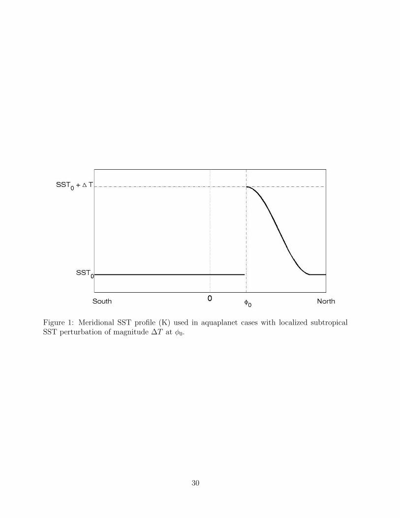
Figure 1: Meridional SST profile (K) used in aquaplanet cases with localized subtropicalSST perturbation of magnitude ∆T at φ0.

30

Figure 2: Steady-state results as a function of subtropical SST forcing for aquaplanet case.Top, absolute global minimum circulation streamfunction strength, kg s−1. Bottom, mini-mum 150 hPa absolute vorticity between 6N and 64N .

31

Figure 3: Steady-state streamfunction for aquaplanet case, 100 day time mean, SST pertur-bation located at φ0 = 16N . Solid contours denote counter-clockwise flow, dashed contoursindicate clockwise flow. Note that contour interval is 4 times greater for the figure onthe right. Left, subthreshold result for ∆T = 1.0K, contour interval 2.5E9kg s−1. Right,supercritical result for ∆T = 2.0K, contour interval 1E10kg s−1.

32

Figure 4: Steady-state streamfunction, 100 day time mean, coastline located at 16N . Solidcontours denote counter-clockwise flow, dashed contours indicate clockwise flow. Top left,subcritical result for THF0 = 130W m−2 with uniform SST, contour interval 5E9kg s−1.Top right, supercritical result for THF0 = 140W m−2 and uniform SST, contour interval5E9kg s−1. Bottom left, aquaplanet case with SST maximum at 8N , contour interval1E10kg s−1. Bottom right, continental case with summer SST THF0 = 140W m−2, contourinterval 1E10kg s−1.

33

Figure 5: Absolute global minimum steady-state streamfunction for aquaplanet case, 100day time mean, SST perturbation at northern hemisphere latitude φ0.

34

Figure 6: Steady-state results as a function of land forcing strength. Continent with uni-formly warm ocean, solid lines with squares; continent with “summer” SST, dot-dash linewith asterisks. Top, absolute global minimum circulation streamfunction strength, kg s−1.Bottom, minimum 150 hPa absolute vorticity between 6N and 64N .

35

Figure 7: Location of maximum monsoon precipitation for steady monsoon as a function ofland surface forcing strength (THF0). Case with coastline at φL = 16N and uniform warmSST.

36

Figure 8: Hovmoeller diagram of precipitation for seasonal cases, contour interval 2.0mm day−1. Left, maximum summer land forcing THF0 = 130W m−2; right, maximumsummer land forcing THF0 = 150W m−2. Day zero occurs at winter solstice, annual meandata over four years of model integration.

37

Figure 9: Summer circulation for seasonal case with THF0 = 150W m−2, contour interval5E9kg s−1. Left, early summer circulation (Day 175); right, late summer circulation (Day250). Day zero occurs at winter solstice.

38

Figure 10: Steady-state fields for continental case with THF0 = 140W m−2 with uniformwarm ocean. Top, streamfunction, contour interval 5E9kg s−1; arrows indicate directionof flow. Center top, zonal wind, contour interval 10m s−1. Center bottom, precipitation,mm day−1. Bottom, 1000 mb moist static energy, 104J .

39

poleward shift

in h maximum

RCE h

increased

LANDOCEAN

Figure 11: Schematic diagram of subcloud moist static energy. Dashed line shows radiativeconvective equilibrium hb, solid line shows hb in the presence of a large-scale circulation. Asthe surface forcing is increased, the radiative-convective equilibrium hb also increases overthe land, but not over the adjacent ocean. Poleward-flowing air from the ocean requiresgreater heating to reach the RCE equilibrium hb, and the hb maximum shifts inland.

40