MonopolyChapter 8

LIPSEY & CHRYSTAL

ECONOMICS 12e

Learning Outcomes

• A monopolist sets marginal cost equal to marginal revenue, but marginal cost is less than price.

• Output is lower under monopoly than under perfect competition.

• Profit can be increased for a monopolist if it is possible to charge different prices to different customers or in separate markets.

• Pure profits exist in the long run under monopoly, so long as there are entry barriers.

• Cartel can increase the profits of colluding firms, but individual members have incentives to break away.

A Single-Price Monopolist: price discrimination• A monopoly is an industry containing a single firm. • The monopoly firm maximises its profits by equating

marginal cost to marginal revenue, which is less than price.

• Production under monopoly is less than it would be under perfect competition, where marginal cost is equated to price.

INTRODUCTION - MONOPOLY

The Allocative Inefficiency of Monopoly• Monopoly is allocatively inefficient. • By producing less than the perfectly competitive output it

transfers some consumers’ surplus to its own profits and also causes deadweight loss of surplus that would have resulted from the output that is not produced.

INTRODUCTION - MONOPOLY

A Multi-Price Monopolist• If a monopolist can discriminate among either different

units or different customers, it will always sell more and earn greater profits than if it must charge a single price.

• For price discrimination to be possible, the seller must be able to distinguish individual units bought by a single buyer or to separate buyers into classes among whom resale is impossible.

INTRODUCTION - MONOPOLY

Long-run Monopoly Equilibrium• A monopoly can earn positive profits in the long run if

there are barriers to entry. • These may be man-made, such as patents or exclusive

franchises, or natural, such as economies of large-scale production.

INTRODUCTION - MONOPOLY

Cartels as Monopolies• The joint profits of all firms in a perfectly competitive

industry can always be increased if they agree to restrict output.

• After agreement is in place, each firm can increase its profits by violating the agreement. If they all do this, profits are reduced to the perfectly competitive level.

INTRODUCTION - MONOPOLY

Total, Average and Marginal Revenue

Pricep=AR

(£)

9.10

9.00

8.90

Quantityq

(£)

9

10

11

Total RevenueTR=p*q

(£)

81.90

90.00

97.90

Marginal RevenueMR = TR/q

(£)

8.10

7.90

The Effect on Revenue of an Increase in Quantity Sold

q1q0

p1

p0

Reduction in revenue

Addition to revenues

Quantity

Pri

ce

· Marginal revenue is less than price because price must be lowered to sell an extra unit.

· For example, consider the marginal revenue of the eleventh unit.· It is total revenue when eleven units are sold (£97.90) minus total

revenue when 10 units are sold (£90.00) which is £7.90.· This is less than the £8.90 at which the eleventh unit is sold

because the price on all previous 10 units must be cut by £0.10 to raise sales by one unit.

Total, Average and Marginal Revenue

· Because the demand curve has a negative slope, marginal revenue is less than price.

· A reduction of price from p0 to p1 increases sales by one unit from q0 to q1 units.

· The revenue from the extra unit sold is shown as the medium blue area.

· To sell this unit, it is necessary to reduce the price on each of the q0 units previously sold.

· The loss in revenue is shown as the dark blue area. · Marginal revenue of the extra unit is equal to the difference

between the two areas.

The Effect on Revenue of an Increase in Quantity Sold

50 100

50 100

250

10

£ p

er u

nit

5

-10

£

0

MR

TR

Elasticity between zero and one

0 < <1

Elasticity greater

than one >1Unity elasticity

=1

AR

Revenue curves and demand elasticity

Quantity

Quantity

· Rising TR, positive MR, and elastic demand all go together.· In this example, for outputs from 0 to 50 units, marginal revenue is

positive, elasticity is greater than unity, and total revenue is rising. · Falling TR negative MR and inelastic demand all go together. In

this example, for outputs from 50 to 100 units, marginal revenue is negative, elasticity is less than unity, and total revenue is falling. (All elasticities refer to absolute not algebraic values.)

Revenue curves and demand elasticity

MC

ATC

AVC

D = ARMR

QuantityProfit-maximizing quantity

£ p

er u

nit

p0

q00

The Equilibrium of a Monopoly

c0

· The monopoly produces the output q0 where marginal revenue equals marginal cost (rule 2).

· At this output, the price of p0 (which is determined by the demand curve) exceeds the average variable cost (rule 1).

· Total profit is the profit per unit of p0-c0 multiplied by the output of q0, which is the yellow area.

The Equilibrium of a Monopoly

MC

D”

D’MR’MR”

q0

p1

p0

0 Quantity

£ p

er u

nit

The same output at different prices

No Supply Curve under Monopoly

· The demand curves D’ and D’’ both have marginal revenue curves that intersect the marginal cost curve at output q0.

· But because the demand curves are different, q0 is sold at:

· p0 when the demand curve is D’ and at p1 when the demand curve is D’’.

· Thus under monopoly there is no unique relation between price and the quantity sold.

No Supply Curve under Monopoly

1

MC [monopoly] = S [competition]

D

Em

q0

Competitive pricep0

0

The deadweight loss of monopoly

Quantity

pm

qm

2

Pri

ce

5

7

6Ec

MR

· At the perfectly competitive equilibrium Ec consumers’ surplus is the sum of the areas 1, 5, and 6.

· When the industry is monopolized, price rises to pm, and consumers surplus falls to area 5.

· Consumers lose area 1 because that output is not produced.· They lose area 6 because the price rise has transferred it to the

monopolist.· Producers’ surplus in the competitive equilibrium is the sum of the

areas 7 and 2.

The deadweight loss of monopoly

· When the market is monopolized and price rises to pm, the surplus area 2 is lost because the output is not produced.

· However the monopolist gains area 6 from consumers. Area 6 is known to be greater than 2 because pm maximizes the monopolist profits.

· Thus although the monopolist gains, society loses areas 1 and 2.· Areas 1 and 2 are the deadweight loss resulting from monopoly and

account for its allocative inefficiency.

The deadweight loss of monopoly

3

1S = MC

D

qd

pd

0

A Price-discriminating Monopolist

Quantity

pm

qm

Pri

ce

MR

qc

2

· Initially the monopolist produces output qm which it sells at pm where MC = MR instead of the competitive output qc where MC equals demand (which is consumers’ marginal utility).

· The deadweight loss is the sum of the three areas labelled 1, 2, and 3.

· A second group of consumers is then isolated from the first (the first group continue to buy qm at pm).

A Price-discriminating Monopolist

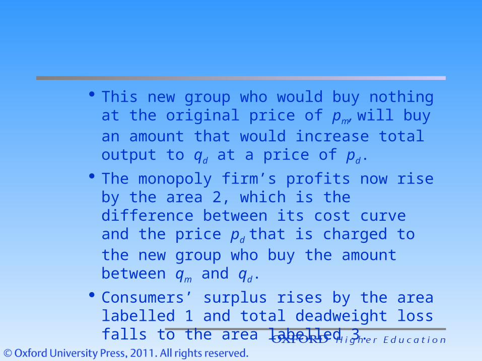
· This new group who would buy nothing at the original price of pm, will buy an amount that would increase total output to qd at a price of pd.

· The monopoly firm’s profits now rise by the area 2, which is the difference between its cost curve and the price pd that is charged to the new group who buy the amount between qm and qd.

· Consumers’ surplus rises by the area labelled 1 and total deadweight loss falls to the area labelled 3.

D

S

E

MR

Q0Q1

p1

p0

0

Quantity [thousands of tons]

£ p

er u

nit

[i]. Market equilibrium [ii]. Firm equilibrium

Conflicting forces affecting cartels

£ p

er u

nit

ATC MC

Ep0

p1

q1 q2q0

Quantity [tons]

Conflicting forces affecting cartels (i) the market

· Initially the market is in competitive equilibrium, with price p0 and quantity Q0.

· The cartel is formed and enforces quotas on individual firms that are sufficient to reduce the industry’s output to Q1, the output that maximizes the joint profits of the cartel members.

· Price rises to p1.

Conflicting forces affecting cartels (ii) an individual firm

· (Note the change in scale from figures (i) and (ii).· Initially the individual firm is producing output q0 and is just

covering its total costs at price p0.

· When the cartel restricts production the typical firm’s quota is q1.

· The firm’s profits rise from zero to the amount shown by the dark blue area.

Conflicting forces affecting cartels (ii) an individual firm

· Once price is raised to p1 however, the individual firm would like to increase output to q2, where marginal cost is equal to the price set by the cartel.

· This would allow the firm to earn profits shown by the blue hatched area.

· But if all firms violate their quotas in this way, industry output will rise above Q1, market price will fall, and the profit earned by each and every firm will fall.