monitoring oil reservoir deformations by measuring ground

Monitoring Oil Reservoir Deformations by Measuring Ground Surface

Movements

by

Kamelia Atefi Monfared

A thesis

presented to the University of Waterloo

in fulfilment of the

thesis requirement for the degree of

Master of Applied Science

in

Civil Engineering

Waterloo, Ontario, Canada, 2009

© Kamelia Atefi Monfared 2009

ii

Author’s Declaration

I hereby declare that I am the sole author of this thesis. This is a true copy of the thesis,

including any required final revisions, as accepted by the examiners.

I understand that my thesis may be made electronically available to the public.

iii

Abstract

It has long been known that any activity that results in changes in subsurface pressure, such as

hydrocarbon production or waste or water reinjection, also causes underground deformations

and movement, which can be described in terms of volumetric changes. Such deformations

induce surface movement, which has a significant environmental impact. Induced surface

deformations are measurable as vertical displacements; horizontal displacements; and tilts,

which are the gradient of the surface deformation. The initial component of this study is a

numerical model developed in C++ to predict and calculate surface deformations based on

assumed subsurface volumetric changes occurring in a reservoir. The model is based on the

unidirectional expansion technique using equations from Okada’s theory of dislocations

(Okada, 1985). A second numerical model calculates subsurface volumetric changes based on

surface deformation measurements, commonly referred to as solving for the inverse case. The

inverse case is an ill-posed problem because the input is comprised of measured values that

contain error. A regularization technique was therefore developed to help solve the ill-posed

problem.

A variety of surface deformation data sets were analyzed in order to determine the surface

deformation input data that would produce the best solution and the optimum reconstruction of

the initial subsurface volumetric changes. Tilt measurements, although very small, were found

to be much better input than vertical displacement data for finding the inverse solution. Even in

an ideal case with 0 % error, tilts result in a smaller RMSE (about 12 % smaller in the case

studied) and thus a better resolution. In realistic cases with error, adding only 0.55 % of the

maximum random error in the surface displacement data affects the back-calculated results to a

significant extent: the RMSE increased by more than 13 times in the case studied. However, in

an identical case using tilt measurements as input, adding 20 % of the maximum surface tilt

value as random error increased the RMSE by 7 times, and remodelling the initial distribution

of the volumetric changes in the subsurface was still possible. The required area of observation

can also be reduced if tilt measurements are used. The optimal input includes tilt measurements

in both directions: dz/dx and dz/dy.

iv

With respect to the number of observation points chosen, when tilts are used with an error of 0

%, very good resolution is obtainable using only 0.4 % of the unknowns as the number of

benchmarks. For example, using only 10 observation points for a reservoir with 2500 elements,

or unknowns resulted in an acceptable reconstruction.

With respect to the sensitivity of the inverse solution to the depth of the reservoir and to the

geometry of the observation grid, the deeper the reservoir, the more ill-posed the problem. The

geometry of the benchmarks also has a significant effect on the solution of the inverse

problem.

v

Acknowledgements

I would like to thank my supervisor at the University of Waterloo, Professor Leo

Ruthenburg, who has provided me with his precious insight and kind support during the

course of my MASc. degree. I am forever grateful for your constant support and kind

encouragement which enabled me to take on new challenging tasks.

I would like to thank my co-supervisor at the University of Waterloo, Professor Giovanni

Cascante for his precious guidance and kind attention throughout the course of my degree.

You provided me with insightful inputs, which helped me improve my presentation,

organizational and time management skills.

I would like to thank my Father, Mr. Amir Pasha Atefi Monfared for his valuable support

and guidance throughout my life. You have always been the greatest mentor and role model

for me. It is because of you that I chose to study Civil Engineering in the first place.

Thanks for your love, support and forever valuable inputs.

I would like to thank my mother, Mrs. Golrokh Tajbakhsh for her unconditional love, and

support. Your constant care, love and attention helped me get through the hardest times of

my life. Thank you for always being there for me and constantly encouraging me every

step of the way.

I would like to thank my sister, Yassaman Atefi who always manages to cheer me up even

in the worst times possible. Your always energetic and joyful character is extremely

powerful and does wonders that you don’t know about. Thank you for always being my

best friend.

vi

Dedication

I would like to dedicate this thesis to my dear parents, Mr. Amir Pasha Atefi Monfared and

Mrs. Golrokh Tajbakhsh who have always been there for me.

vii

Table of Contents

Author’s Declaration ................................................................................................................................. ii

Abstract ..................................................................................................................................................... iii

Acknowledgements ................................................................................................................................... v

Dedication ................................................................................................................................................. vi

Table of Contents ..................................................................................................................................... vii

List of Figures ............................................................................................................................................ x

List of Tables .......................................................................................................................................... xiii

1. Introduction ........................................................................................................................................... 1

2. Literature Review .................................................................................................................................. 4

3. Factors Affecting the Movement of the Ground Surface..................................................................... 23

3.1 Geological terminology ................................................................................................................. 25

3.1.1 Definition of a reservoir .......................................................................................................... 25

3.1.2 Reservoir materials ................................................................................................................. 26

3.2 Mechanical properties of a reservoir and the compaction subsidence mechanism that occurs due

to oil withdrawal .................................................................................................................................. 26

3.2.1 Parameters affecting reservoir compaction ............................................................................. 29

3.3 Methods of monitoring reservoir compaction (subsurface monitoring) ........................................ 32

3.4 Overburden material and the degree to which subsurface compaction is transferred to the surface

............................................................................................................................................................. 33

3.5 Surface deformation monitoring .................................................................................................... 34

3.5.1 Global positioning system (GPS) ........................................................................................... 35

3.5.2 Interferometric synthetic aperture radar (InSAR) ................................................................... 35

3.5.3 Tilt meter monitoring .............................................................................................................. 35

3.5.4 Levelling and distance survey data ......................................................................................... 36

4. Mathematical Approach....................................................................................................................... 37

4.1 Direct case ..................................................................................................................................... 37

4.2 Inverse case .................................................................................................................................... 47

4.3 Ill-posed problem ........................................................................................................................... 49

4.4 Ill-posed problems: the inverse case .............................................................................................. 53

4.5 Regularization technique ............................................................................................................... 57

4.5.1 Defining 𝛽 ............................................................................................................................... 59

4.5.2 Construction of the regularization operator ............................................................................ 60

viii

4.6 Calculating the general matrix equation form of the problem ....................................................... 66

4.7 Solving the matrix equation ........................................................................................................... 69

4.7.1 Singular value decomposition method .................................................................................... 69

5.0 Modeling Technique .......................................................................................................................... 72

5.1 The direct case ............................................................................................................................... 72

5.2 The inverse case ............................................................................................................................. 73

5.2.1 Using only one data set from each observation point as input ............................................... 73

5.2.2 Using two or more data sets from each observation point ...................................................... 74

6.0 Cases considered and results ............................................................................................................. 81

6.1 Verifying the code ......................................................................................................................... 81

6.2 Studying the effect of depth on the ill-posed nature of the problem ............................................. 83

6.2.1 Case 1 ..................................................................................................................................... 83

6.3 Finding the best surface deformation data as input that results in the best resolution ................... 89

6.3.1 Comparing results from displacement and tilts assuming no error present ............................ 89

6.3.2 Results of a comparison of cases 2 -- 6 .................................................................................... 105

6.4 Limiting the area range for observation points using tilts ........................................................... 106

6.4.1 Case 7 ................................................................................................................................... 106

6.5 Error in the input data .................................................................................................................. 110

6.5.1 The effect of the error present in vertical displacement measurements on the resolution of the

ill-posed problem ........................................................................................................................... 110

6.5.2 The effect of the error present in tilt measurements on the resolution of the ill-posed problem

....................................................................................................................................................... 114

6.5.3 The effect of error present in vertical displacement + tilts1+2 on the resolution of the ill-

posed problem ................................................................................................................................ 119

6.6 Effect of the number of observation points on the inverse resolution ......................................... 123

6.6.1 Omitting random points using tilt1+ 2 + displacement with 0 % error as input ................... 124

6.7 The effect of the distribution of the observation points on the resolution of the inverse problem

........................................................................................................................................................... 133

6.7.1 0% error present in the observation data .............................................................................. 134

6.8 The effect of the presence of error in the data combined with the omission of observation points

........................................................................................................................................................... 140

6.8.1 Error of 10 % ........................................................................................................................ 140

6.8.1.1 Case 34: ............................................................................................................................. 140

6.8.1.2 Case 35 .............................................................................................................................. 141

ix

6.8.1.3 Case 36 .............................................................................................................................. 142

6.8.1.4 Case 37 .............................................................................................................................. 143

6.8.1.5 Case 38 .............................................................................................................................. 144

6.8.1.6 Case 39 .............................................................................................................................. 145

6.8.1.7 Case 40 .............................................................................................................................. 146

6.8.1.8 Case 41: ............................................................................................................................. 147

6.8.2 Case of 5% error ................................................................................................................... 149

6.8.3 Case of 3 % error .................................................................................................................. 150

6.8.4 20 observation points with 1 % error: case 44 ...................................................................... 152

7.0 Conclusions ..................................................................................................................................... 156

8. Future work and recommendations ................................................................................................... 158

References ............................................................................................................................................. 159

Appendix ............................................................................................................................................... 162

Appendix I: Calculating the L matrix .................................................................................................... 162

Appendix II: Graphs: limiting observation area .................................................................................... 166

Appendix III: Graphs; error in input data .............................................................................................. 170

Appendix IV: Graphs; volume change calculations; omitting points: ................................................... 176

Appendix V: Graphs; studying the effect of observation distribution .................................................. 198

Appendix VI: the numerical modeling of the inverse solution in C++ ................................................. 228

x

List of Figures

Figure 1: A comparison of the number of holes visible in the outer part of the protective wall in the two

photos of the 2/4T platform at the Ekofisk field reveals the extensive vertical subsidence (Hermansen et

al., 2000) .................................................................................................................................................... 6

Figure 2 : Illustration of the way in which surface deformation graphs can be used in order to study

volumetric changes in the subsurface (Dusseault et al., 2002). ............................................................... 16

Figure 3: Surface deformation field for a waste injection project (Rothenburg et al., 1994). ................. 16

Figure 4: Surface deformation as the result of subsurface volume change (Rothenburg et al., 1994). ... 18

Figure 5: Surface deformation as the result of waste injection at different depths (Rothenburg et al.,

1994). ....................................................................................................................................................... 18

Figure 6: Evolution of ponding in the Wairakei stream at the centre of the subsidence bowl. The

photograph on left was taken in 1981, and the photograph on the right was taken in 1997at almost the

same location (Allis, 2000). ..................................................................................................................... 21

Figure 7: The approximate deformation field as a result of a point source of volume change at depth d.

................................................................................................................................................................. 23

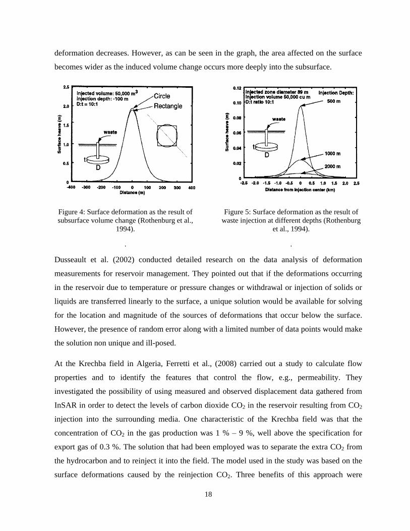
Figure 8: Void ratio of a soil sample plotted against the effective stress from the oedometer test ......... 28

Figure 9: Change in volume modeled as a point of expansion in the subsurface: nucleus of strain

approach................................................................................................................................................... 37

Figure 10: Nucleus of strain points in reservoir elements. ...................................................................... 38

Figure 11: Shape of the reservoir assumed for modeling. ....................................................................... 39

Figure 12: A general form of reservoir plate with a dip angle of 𝛿, a length of L, a width of W, a depth

of –d, and an Azimuth of 0ᵒ (Okada, 1985). ............................................................................................ 40

Figure 13: Illustration of the mathematical approach of the surface deformation that occurs due to a

subsurface volume change (Bilak, 1989). ................................................................................................ 49

Figure 14: The effect of the value of 𝛽 on the solution of the inverse problem (Dusseault et al., 2002). 60

Figure 15: Results of the inverse calculations, showing a large number of jumps, especially at the corner

points; the solution is therefore not smooth (Rothenburg, 2009, personal communication). .................. 63

Figure 16: Surface deformation due to volume change at a very shallow depth. .................................... 83

Figure 17: Distribution of volume change assigned to the test reservoir. ............................................... 88

Figure 18: Induced vertical deformations due to reservoir’s volume change .......................................... 89

Figure 19: The reservoir to be modeled and the resulting induced deformation field on the surface due

to reservoir volume change ...................................................................................................................... 90

Figure 20: MSE and RMSE plotted against 𝛽: Case 2 ............................................................................ 91

Figure 21: Δv for the first six rows of the reservoir; Case2. .................................................................... 93

Figure 22: Δv for the rows 25 to 30 of the reservoir; Case2. ................................................................... 94


Figure 24: Δv for the first six rows; Case 3. ............................................................................................ 96

Figure 25: Δv for rows 25 to 30 of the reservoir; Case 3. ....................................................................... 97


Figure 27: MSE and RMSE and the third factor used plotted against 𝛽, Case 5 ..................................... 99

Figure 28: Δv for the first six of the reservoir; Case 5. ......................................................................... 100

Figure 29: Δv for the rows 25 to 30 of the reservoir; Case 5. ................................................................ 101

xi

Figure 30: Δv for the first six rows of the reservoir; Case 6. ................................................................. 103


Figure 32: Cutting out a part of data by limiting the observation area on the surface and thus using only

data from part of the observation field .................................................................................................. 107

Figure 33: Volume changes in volume in the first five rows of the reservoir, with the observation field

limited .................................................................................................................................................... 109

Figure 34: MSE and RMSE plotted against 𝛽: Case 8 .......................................................................... 111

Figure 35: Δv for the first six rows of the reservoir; Case 8. ................................................................. 112


Figure 37: Results of RMSE from the inverse solution of different cases using tilt1+tilt2 with error

plotted against 𝛽. ................................................................................................................................... 115

Figure 38: Δv for the first six rows of the reservoir; Case 16. ............................................................... 117

Figure 39: Δv for the rows 25 to 30 of the reservoir; Case 16. .............................................................. 118

Figure 40: MSE and RMSE plotted against 𝛽: Case 17 ........................................................................ 120



Figure 43: MSE and RMSE plotted against 𝛽: Case 18. ....................................................................... 125










Figure 53: RMSE plotted against the number of observation points. .................................................... 132

Figure 54: Plan of reservoir with observation points distributed in two rows, one vertical and one

horizontal, which meet at the corner above the reservoir. ..................................................................... 135

Figure 55: MSE and RMSE for different values of 𝛽s: Case 29 ........................................................... 135

Figure 56: Plan of reservoir with observation points distributed in two rows, one horizontal and one

vertical, which cross at the centre of the reservoir. ............................................................................... 136




Figure 60: MSE and RMSE for different values of 𝛽s: Case33. .......................................................... 139


Figure 62: MSE and RMSE for different values of 𝛽s: Case 35. ......................................................... 142

Figure 63: MSE and RMSE for different values of 𝛽s: Case36. ........................................................... 143

Figure 64: Plan of the reservoir with observation points distributed in three vertical and three horizontal

rows crossing above the centre of the reservoir. .................................................................................... 143

Figure 65: MSE and RMSE for different values of 𝛽s: Case 36. .......................................................... 144

Figure 66: Plan of the reservoir with the observation points distributed in three vertical and three

horizontal rows above the reservoir. ...................................................................................................... 144

xii

Figure 67: MSE and RMSE for different values of 𝛽s: Case 38 ........................................................... 145

Figure 68: Plan of the reservoir with observation points distributed in six vertical rows above the centre

of the reservoir. ...................................................................................................................................... 145


Figure 70: Plan of the reservoir with observation points distributed in two vertical rows above the centre

of the reservoir. ...................................................................................................................................... 146



Figure 73: It can be seen although MSE being very close, the distribution is totally different. ............ 149



Figure 76: Observation grid of 20 points. .............................................................................................. 152



xiii

List of Tables

Table 1: Properties of common subsiding oil reservoirs (Nagel, 2001). ................................................. 31

Table 2: Verifying the results using Okada’s numerical checklist .......................................................... 82

Table 3: Results of back-calculations when 𝛽=0 for various depths. ...................................................... 84

Table 4: Results of back-calculations for a depth=5 m. .......................................................................... 85

Table 5: Results of back-calculations for a depth=10 m. ........................................................................ 85



Table 8: Comparison of results from identical cases for which input deformation data varied. ........... 105

Table 9: MSE and RMSE for different 𝛽s: tilt1 and tilt2 ...................................................................... 108

Table 10: Comparison of results for a limited area of observation points ............................................. 109

Table 11: Minimum MSE for different error percentages used as input ............................................... 116

Table 12: Results summarized to show the effect of error in the observation data. .............................. 123

Table 13: Comparison of results to show the effect of the number of observation points. ................... 132

Table 14: Comparison of the results showing the effect of the distribution of observation points. ..... 137

Table 15: Comparison of the results of cases 30, 32,and 33. ............................................................... 139

Table 16: Summary of results with respect to the effect of the number and distribution of observation

points along with the error present in the observation data. .................................................................. 148

Table 17: Comparison of results: the effect of error for the best benchmark distribution .................... 151

1

1. Introduction

Near-surface deformations induced by subsurface movements have been identified as an

important operational problem for many years. Subsurface movements can be caused by a

number of activities, such as oil production and steam or waste injection. Any activity that

causes subsurface pressure changes generates displacement zones and, consequently, surface

movements. Hence, the withdrawal or injection of any kind of fluid or material into the

subsurface induces subsurface volume changes that cause deformations and displacements at

ground level. These surface deformations are typically measured as vertical displacements;

horizontal displacements; and tilts, or ground rotations, with respect to the vertical.

Excessive surface deformations can result in significant economic losses because of the failure

of underground utility lines, well casings, and pipelines, as well as structural damage generated

by seawater intrusions and foundation settlements (Hu et al., 2004). The induced land

subsidence can exceed several meters; however, in some cases, even small subsurface

deformations can cause significant damage to the surrounding environment (Nagel, 2001). In

the Netherlands, for example, where large areas of dry land are below sea level and protected

by surrounding dikes, even a small subsidence could result in disaster (Nagel, 2001). Wetland

loss is another phenomenon caused by either natural or human-induced subsidence, or, given

their complex relationship, by a combination of both.

Extensive research has been performed worldwide in this area because of the wide distribution

of regions affected by land deformations, which have a severe impact on the environment. In

most studies, the main objective has been to predict surface deformations so that preventive

action can be taken as quickly as possible in order to minimize damage, optimize production

and injection, and develop better monitoring strategies. Another factor, however, is that surface

deformations are measurable and depend on subsurface movements and deformations (Vasco,

2004; Segall, 1985; Geertsma, 1957). Thus, the measurement and monitoring of surface

deformations can be used in the modeling and tracking of subsurface deformations. This

approach is especially useful in fast-paced projects such as waste or steam injection, in which

the continuous monitoring of subsurface deformation is of great value. The evaluation of

subsurface deformation using surface deformation data is called an inverse problem. The

2

resulting subsurface deformation data can be used to determine steam concentration zones in

steam injection projects, to model deformations and fracture movements in waste injection

projects, to manage and optimize injection and production patterns in reservoirs, and to

monitor the reaction of a reservoir to production and enhanced recovery processes in the oil

and gas industry. In addition, important information can be derived from this subsurface data

for tracking the areas of extraction and injection of fluids. Identifying this information is

critical in determining whether the reinjected material is remaining in its desired target

locations (Dusseault et al., 2002).

Unfortunately, detailed information about subsurface deformations and movements is

unavailable for modelling subsurface movements. However, an analog of St. Venant’s

principle in mechanics applies: if the effect of a force or deformation located at a distance from

the point of interest is under study, the details of this force or deformation do not have a

significant effect on the induced deformation field. Thus, two approaches are commonly used

to reconstruct subsurface deformations:

Nucleus of strain approach: the subsurface deformations are modeled by representing

discontinuities as single points that are expanding or compacting in the subsurface and

that represent expansion or compaction, respectively.

Unidirectional expansion: an approach that is based on equations from the theory of

dislocations (Okada, 1985): Okada’s solution models concentrated on expansion or

compaction that occurs in one direction.

The unidirectional expansion technique is used in this study. This method typically provides

better simulations of the behaviour of the reservoir because the thickness of the reservoir is

small in comparison to its depth and width. Thus, the induced deformations are primarily in

one direction: vertical.

For the first component of this research, a forward numerical model was developed in C++

based on Okada’s formulas. This computer program calculates surface deformations from

given changes in volume in the subsurface. The main types of input to the program are the

geometry of the reservoir (depth, width, length, azimuth and dip angle), the number of

observation points, the subsurface volume changes, and the elastic properties of the media

3

(Lamé’s constants). The output of the program is the vertical displacements and ground tilts at

each observation point. However, the main focus of this work was to evaluate the subsurface

volumetric changes given the field of surface displacements (e.g., the solution of the inverse

problem). Like so many other inverse problems, this inverse problem is an ill-posed problem;

thus, the solution is significantly affected by minor inaccuracies in the measured data. These

inaccuracies are also present in the input data because of the measurement errors, and the

solutions of ill-posed problems are therefore not unique. Consequently, the second and main

part of this thesis is focused on solving the inverse problem.

Surface deformations computed in the first part of the research for a given set of volume

changes are used as input data. The subsurface volume changes are then calculated using the

inverse model. For the verification of the model, the results are then compared to the initial

assumed volume changes assumed.

Forward and inverse models have been previously studied and reported on in the literature.

Some models for the case of extreme uncertainties are based on the nucleus of strain approach,

in which subsurface volume changes are modeled at random locations (Dusseault et al., 1993;

Kroon et al., 2008; Vasco et al., 2002). The solution in these cases involves minimizing the

parameters of these random variables so that the observed deformation field can be

reconstructed. The approach in this thesis is based on Okada’s unidirectional deformations in

well-defined locations. The ground surface displacement data considered in this study include

both vertical deformations and tilts. Previous studies were based on measurements of surface

displacements only (e.g., Bilak, 1989). The goal of this study was to identify a set of

measurements that would result in the best resolution in the solution of the inverse problem.

The sensitivity of the inverse solution to the depth of the source of deformation, the locations

of the surface measurements, and the measurement error were also studied in detail, and the

results are presented in this thesis.

4

2. Literature Review

Subsurface volumetric change has long been induced by human activities such as oil

production, steam reinjection, waste reinjection, and mining. Such types of activities take place

all over the world and have a significant environmental impact. In some instances, ground

deformations can result in significant structural damage. These phenomena have been the

subject of extensive study on the part of oil companies and individual researchers over the past

50 years. The studies have examined aspects of surface deformation, natural and manmade

causes of deformation, deformations due to the extraction of fluids or solids, the measurement

and monitoring of deformations, the theory and modeling of deformations, the prediction of

surface deformations, the social effects of deformations, the environmental consequences of

deformations, methods of preventing or controlling induced deformations, the inverse case, and

the obtaining of subsurface deformation data based on surface displacement.

Two of the major causes of surface deformation have been oil and gas production, and water

withdrawal. Surface deformation due to the withdrawal of water, oil, or gas has been observed

and recorded in the literature for more than a decade. The first reported cases related to

subsidence caused by underground water withdrawal, one of the earliest cases of which took

place in the Osaka field in Japan in 1885. Also caused by water withdrawal was the 3 m of

subsidence, with a subsidence bowl of 10 000 𝐾𝑚2, observed as early as 1906 in the Houston

Galveston area. Other early cases were reported in London, England, in 1865 and in Mexico

City beginning in 1929 (Gurevich et al., 1993). In the oil industry, one of the earliest cases of

subsidence was first noted at the Goose Creek oil field in Texas, USA, in 1918 (Chan et al.,

2007). Roadway subsidence due to oil recovery was also observed on Hogg Island and along

Tabbs Bay, and surface faulting was first documented in the town of Pelley as early as 1918

(Nagel, 2001).

In the oil and gas industry however, the first major case of surface deformation to be widely

recognized was observed at the Wilmington field largely because of the significant amount of

land subsidence and the enormous cost of the resulting damage. Wilmington field, located near

Los Angeles, California, was first discovered in 1932, with production beginning in 1936.

Indications of subsidence were observed in the following years, but the first subsidence due to

5

production in this field was measured and recorded in 1940. By 1970, more than $100 million

had been spent to evaluate the damage due to the subsidence, to protect and compensate for the

damages due to subsidence. The total vertical subsidence reached more than 9 m by 1968. It

was noted that the oil company was required to maintain a water injection rate of 105 % of the

production value in order to prevent further subsidence due to oil withdrawal (Nagel, 2001).

The Ekofisk field in the Norwegian sector of the North Sea, first discovered in 1969, is one of

the best known cases in the oil and petroleum industry because of the immense subsidence that

has resulted from the oil withdrawal. The reservoir is composed of two fractured chalk

horizons from which oil is extracted. Its depth is about 2927 m, and its thickness varies from

approximately 107 to 152 m. The porosity of the reservoir ranges from 30 % to a maximum of

48 %. Beneath this chalk reservoir, lies a Tor Formation with a thickness of approximately 77

to 153 m and a porosity of 30 % to 40 % (Hermansen et al., 2000). The first test production at

the Ekofisk field began in 1971. Oil production peaked in 1976 at a rate of 350,000 STB/D.

Gas injectors were also built, and all the gas produced was reinjected until pipelines were

installed in 1977 to transfer the gas to Germany.

Initially, before oil production began, engineers did not expect any subsidence in the seabed.

However, this prediction was incorrect, and 3.05 m of seabed subsidence was measured in

1984. Two images that were taken 9 years apart and that show the degree of this deformation

are provided in Figure 1.

6

Figure 1: A comparison of the number of holes visible in the outer part of the protective wall in

the two photos of the 2/4T platform at the Ekofisk field reveals the extensive vertical

subsidence (Hermansen et al., 2000)

Laboratory results indicated that a significant additional amount of oil could be mobilized if

high enough gradients existed in the field. In 1983, the company therefore decided to flood the

northern Tor formation with water. This massive flooding of the Ekofisk field resulted in a

significant increase in oil production and a substantial drop in the gas-to-oil ratio (GOR). The

deformation of the reservoir in this chalk formation resulted in casing failures in two-thirds of

the wells in Ekofisk (Bruno et al., 1992) and in the failure of a number of them (Du et al.,

2001; Nagel, 2001; Hermansen et al., 2000; Bruno et al., 1992).

The vertical displacement rates on the seafloor were also so enormous that in 1987 it was

decided to jack up the offshore platforms in order to protect the steel platforms and concrete

storage tanks, especially in severe weather; to prevent the structure from sinking beneath sea

level; and to maintain a constant platform air gap (Nagel, 2001). In 1989, a concrete protective

barrier was designed, and a new phase, the Ekofisk II, was redeveloped as a means of

compensating for the huge amounts of subsidence (Nagel, 2001). Also due to the excess

tension and compression with respect to the pipelines in the subsiding Ekofisk bowl, 63 km of

new pipeline has to be replaced during the Ekofisk II redevelopment. The following actions

taken by the company led to an increase in oil recovery: extensive water flooding (a total of 2

billion barrels of water were injected in the first 10 years of the water flooding operations),

effective well monitoring, compaction drive energy, the Ekofisk redevelopment, and the

overall optimization of field methods and techniques (Hermansen et al., 2000).

7

The South Belridge field in California is a diatomite reservoir, which is characterized by very

high porosity and low permeability, resulting in very high compactions of the reservoir rock.

Compaction in this field caused numerous tension fractures on the surface and numerous

casing failures (Dusseault et al., 2002). During the 1980s, these failures became so severe that

15 % – 20 % of the well casings failed each year (Nagel, 2001).

The Lost Hills field, located along the west side of the San Joaquin Valley in California, is

another diatomite reservoir where petroleum production has led to surface subsidence at rates

as high as 30 cm per year and damage to hundreds of wells (Du et al.,2001; Bruno et al., 1992).

More than 20 m of changes in elevation were observed during 30 years of extensive oil and gas

production in the Louisiana Coastal Zone area. Land loss in this area has also been reported to

be 80% of the total land loss in the United States since the 1930s, which has a major social,

economic, environmental, and ecosystem impact. The height of the land loss, which occurred

in the 1970s, coincided with the peak of oil and gas production in the area (Chan et al., 2007).

While some reservoirs like the Ekofisk field or the Wilmington field are well known for the

large amounts of land deformation induced by hydrocarbon production, in many cases, very

small displacements can also present serious challenges and can result in disaster. In

Venezuela, for example, induced land subsidence due to reservoir compaction resulted in

severe flooding of more than 450 𝑘𝑚2 of land near the coast of Lake Maracaibo. This field is

located in an area called the Bolivar Coast where subsidence had occurred due to oil

production in several fields as early as 1929. By 1988, the subsidence in these fields exceeded

5 m, and by the following year, 150 km of dikes had been built, for which the annual cost of

maintenance was estimated to be $5 million.

The Groningen gas field in the Netherlands is another case in which even small induced land

subsidence can be very challenging. The subsidence in this field was reported to be only in the

order of tens of centimetres. However, because large areas in the Netherlands are below sea

level and are protected by dikes, these induced deformations can cause tension in the

surrounding dikes, which could be disastrous (Nagel, 2001). Surface monitoring has thus

become very important in this region.

8

The abovementioned cases are important examples of observed cases of surface deformations

induced as a result of oil and gas production. In these cases the intention is usually to predict

the deformations and thus solve the problems involved in that specific case. However, as

mentioned, in some cases, if water flooding or steam reinjection is applied during production,

then keeping track of and controlling the induced volumetric changes in the subsurface would

become important. Thus surface monitoring to keep track of induced surface deformations

would be required. Based on this surface deformation data, subsurface movements and

volumetric changes can be modeled. This is referred to as solving for the inverse case.

Many cases of induced surface deformation that have been observed are due to underground

water withdrawal, geysers, geothermal fields, steam reinjection projects, and waste reinjection.

The general mechanism and occurrence of induced surface deformations is believed to be

similar regardless of the type of the reservoir involved.

The literature contains numerous articles about induced land deformation. Some have focused

on specific fields while others have presented a broader and more general analysis.

In 1957 Geertsma conducted extensive research on the similarities between temperature

distribution in a thermo elastic material and liquid pressure distribution in a saturated porous

medium in two cases of plane strain and plane stress. Plane strain refers to cases in which one

dimension is much larger than the other dimension, e.g., a tunnel. Plane stress, however, refers

to cases in which one dimension is much smaller than the two other dimensions, such as a

plate. The latter case is relevant for reservoirs and how they are modeled for numerical or finite

element reconstruction. In both cases, one of the major stresses is equal to zero. Biot (1956)

pointed out that in the same way pore compressibility affects the distribution of pore pressure,

the dilation of the solid also appears as an interaction term in the temperature distribution

equation . Based on this fact, Geertsma (1957) tried to express the constants in pore pressure

distribution using the theory of pore and rock bulk volume variations for porous rocks. From a

comparison of the completed equation for temperature distribution in thermo elastic materials

and the distribution of liquid pressure, it can be seen that liquid mobility in pores is relevant to

the heat conductivity, the compressibility replaces specific heat, and the compressibility ratio is

replaced by thermal expansion.

9

A great deal of research has been conducted with respect to the mechanism of surface

deformation due to changes in the subsurface volume and focusing on the individual specific

cases. The mechanism of and factors in surface subsidence were studied with respect to well-

known cases. The following are examples from the literature.

Hermansen et al., (1998) published an article about the experience at the Ekofisk field after 10

years of water flooding the field to prevent large amounts of subsidence due to oil production

in the seabed. The main focus of this research was on the water flooding and related

challenges. The main difficulty with the water flooding, which was the primary method of

compensating for the subsidence, was that uncertainties had to be predicted before massive

amounts of water were injected into the highly fractured chalk formation: recovery potential,

sweep efficiency, water injectivity, and rock stability. The results of the years of wide water

injection were a substantial increase in the oil production of many of the wells and a significant

drop in the gas to oil ratio (GOR). Only in wells affected by faults and fracture trends did water

breakthrough occur. This study pointed out the importance of detailed mapping of faults and

fractures and also of acquiring an understanding of the major stress orientations so that the

permeability anisotropy could be determined in order to prevent or minimize water

breakthrough.

The same study also examined reservoir compaction and land subsidence. It was initially

thought that subsidence is solely the result of an increase in vertical stress due to the depletion

of pore pressure as a result of oil withdrawal. However, even after the field was flooded with

water and the pore pressure was kept constant, the subsidence rate, although reduced,

continued to remain at fair constant. Therefore, another mechanism for the compaction that

occurred in the Ekofisk field was sought. The researchers found that areas that experienced

increasing water saturation, e.g., due to water breakthrough, even under constant effective

stress, also experienced significant amounts of subsidence whereas other areas subjected to

constant pressure due to maintenance operations had zero subsidence. Therefore, the

weakening of the chalk material due to contact with “non-equilibrium” cold seawater was

recognized as another mechanism that caused subsidence in the Ekofisk field. Thus, the

subsidence in the Ekofisk field was found to be due to two major factors: an increase in the

10

effective stress due to a drop in pore pressure and an increase in water saturation in the chalk

matrix even in conditions of constant pore pressure.

Also mentioned in this paper were developments suggested and tested for the Ekofisk field as

methods of compensating for the induced rates of subsidence caused by the increase in water

saturation inside the chalk matrix: injecting gas rather than water, using a water-alternating-gas

(WAG) technique, and surfactant injection. In 1996, WAG was applied, and gas injection was

tested in one of the wells in which water had previously been injected for about 5 years. The

test was unsuccessful, and the injection rate dropped to zero in a matter of hours. The bottom

borehole temperatures were found to be 54℉(≈ 12.2℃), which is well below the hydrate

formation temperature at the reservoir pressure. A temperature contour was then calculated

around the well hole, and it was revealed that the hydrate-forming conditions existed at a

distance of several hundreds of metres from the well hole. This finding was in accordance with

what would be expected after five years of cold water injection into the well. The next

solutions suggested were gas injection with heated water.

In 1993 Li Chin considered another mechanism as a cause of the compaction in the Ekofisk

reservoir: shear-induced compaction. This suggestion led to a significant effort to predict and

model the Ekofisk reservoir compaction and surface subsidence using finite element models.

The main mechanism used to simulate reservoir compaction in these models was pore pressure

drop due to production. At the time, the results seemed to be in accordance with the observed

data, but over time, even after injections were made to slow down the subsidence rate and

although the subsidence rate was much less than the previous levels, the observations still

indicated larger values than those produced by the models, in which the main mechanism, pore

pressure drop, was being controlled by the injections. Another mechanism therefore seemed to

be involved.

Uniaxial strain and triaxial stress compaction tests were performed on samples from the

Ekofisk reservoir, both on samples from the upper formation, which has a high quartz content,

and also on samples from the lower Tor formation, which has a low quartz content. The results

showed a 𝐾0 value of 0.2 rather than 0.5. In Mohr-Coulomb cycles, this indicates much greater

growth. This low 𝐾0 value shows that as production proceeded, pore pressure dropped, and

thus deviatoric stresses increased significantly along with the development of shear stresses,

11

which caused the rock to fracture. Based on the results and the in-situ stresses calculated, it

was deduced that slipping on fractures will also occur because of pressure depletion in the

reservoir.

The changes that occur during repressurization were also studied. During repressurization due

to water or gas injection, pore pressure increases, causing a decrease in the effective stresses.

This effect can also be seen in a Mohr-Coulomb cycle, in which decreasing the effective

stresses forces the sample to the left, into the failure zone when 𝐾0= 0.2, whereas for 𝐾0 = 0.5,

which is the normal case, failure would not be as intense. Measurements from the injection

well and the compaction observations showed that a pressure increase resulting from

reinjection can cause additional compaction of the affected chalk reservoir formation.

The arch effect of the overburden was also studied, and it was observed that the stresses

induced from deformations were greatest on the edges where there is a distinct transition from

high- to low-porosity chalk. Based on the observations of the Ekofisk field, since the

subsidence was more than predicted, it was determined that the chalk is fractured either

naturally or due to the shear stresses that result during injection or production procedures, and

thus, in this case, shear stresses are also a cause of compaction mechanism.

Due to the constraints on displacement in the field which are difficult to reproduce in the lab,

the actual 𝐾0 value is lower than that of in the lab. For modeling purposes, the most important

point determined from this case was that the stress path after the pore pressure drop inside the

reservoir should be such that 𝐾0, which is the ratio of change in horizontal effective stress to

the change in vertical effective stress, be 0.2 so that field conditions are represented correctly.

The stress path in the model was controlled by 𝐾0 as observed in the field. Once the Mohr

cycle reaches a critical angle, the coding automatically changes its stress-strain curve to a

weaker curve. The model is programmed in such a way that, with the initial conditions (initial

vertical and horizontal and pore pressures) under gravitational loads, the K value in the

program is set to 0.5. As soon as production is started, K is set to 0.2.This value is then

maintained at a constant level as long as the vertical strain is compressive or as long as

production is in progress, and thus a decrease in pore pressure and an increase in the effective

vertical stress is occurring. As soon as the pore pressure increases, which may be as a result of

an injection inside the reservoir, K would be set to 0.5. This value is then maintained until

12

another change occurs in the direction of the strain. Of course, identifying the K value near

areas such as injection wells, where pressure increases may be in the order of tens of MPa, is of

great importance. The two most important parameters used in this modelling, which were

controlled by input data, were the position of the critical envelope and the weakening factor

used to determine a weakened stress-strain curve.

To expand oil and gas production development in the Lost Hills field in California, an

extensive program was implemented by Bruno et al. (1992): laboratory tests and rock property

measurements, monitoring and studying of subsurface compaction and the resulting surface

deformations, and analytical and numerical modelling. Surface deformation due to oil

production was a problem in this field because of the soft and porous formation of the rock

matrix and the thick and shallow nature of the reservoir. Using GPS, data related to surface

deformation was gathered at three-month intervals from 1989 to 1991. It was observed that

during this period, subsidence was linearly related to the total fluid production in the centre of

the field. With respect to the subsurface, approximate measurements of the compaction of the

rock matrix were obtained using radioactive bullet logs in one well and gamma logs of natural

markers in other wells. These results indicated compaction of about 61 cm from 1990 to 1991.

A detailed lithology was recorded for the Lost Hills field, and the layers and formations and

their properties were all studied carefully, along with the mechanical properties of the rock.

The two most important factors affecting reservoir compaction mentioned in this research were

pore volume compressibility and bulk volume compressibility (Bruno et al., 1992). Although it

is said that these compressibility factors are related to other compressibility and elastic

constants and can be well defined, in diatomite reservoirs this is not the case. Because the

deformation of a diatomite reservoir has been determined to be inelastic at all stress levels,

these factors can be measured empirically from lab tests under fully drained conditions.

Diatomite samples from Lost Hills showed slightly increased compressibility when the

effective stress exceeded 1000-1100 psi. Triaxial tests were carried out on undisturbed

diatomite samples. Based on the results, the stress-strain, loading, and unloading graphs were

plotted. The slope of the bulk volume strain plotted against that of the hydrostatic stress

represents a measure of the bulk compressibility. The unloading curve shows that the material

remains stiff when unloaded, thus indicating irreversible damage and deformation. From this

13

stiffer unloading behaviour, it was determined that water reinjection was needed in order to

compensate for irreversible subsidence due to oil withdrawal. These tests revealed that

compressibility increased as the effective stress exceeded 1200 Psi.

Core samples were also taken from the overburden material lying over the diatomite reservoir,

and triaxial tests were carried out in order to determine the stiffness and failure properties of

the overlying material. A finite element model was applied in order to calculate and predict the

surface subsidence and well casing failure due to oil withdrawal. For the modelling of the field,

several assumptions were made; the field is long and narrow, so a symmetrical line was

assumed. This geological model covered up to 1829 m in depth and 305 m in half width up to

the symmetrical line, and four materials were modeled: sand and gravels (upper sands),

siltstones and shales, diatomite, and shale. The purpose of the model was not provide precise

calculation of future subsidence but rather to provide an idea of what might occur, along with

an estimate of the damage to a well, areas of potential well failure, potential fault movements,

and optimum injection of water to flood the reservoir. The deformations and shear stress

induced in the overburden in this model were calculated based on a variety of assumed

pressure distributions inside the reservoir. The shale formation underneath the reservoir was

modeled as an elastic material. The overlying siltstone and sand layers were modeled based on

the Drucker-Prager yield condition.

More than 20 m of change in elevation was observed in the Louisiana Coastal Zone over 30

years, during which extensive gas and oil production was carried out in the area. In 2007,

studies were conducted on the role of hydrocarbon production in land deformation and fault

reactivation in the Louisiana Coastal Zone by Alvin W. Chan et al. (2007). The values for

subsidence due to oil production calculated by the numerical program were below half of those

observed in the field. Another factor was therefore suspected of resulting in the subsidence that

was occurring in the field, so compaction-induced fault slip along the Golden Meadow fault at

the northern edge of the reservoirs was studied as a possibility. The researchers listed the

following factors that cause submergence of wetlands: consolidation of the Mississippi River

sediment, which might have a first order effect on subsidence; regional subsidence due to the

loading of sediments; changes in sea level; movement of faults; hydrocarbon production; and

reservoir compaction. The first four mechanisms were mentioned to cause subsidence of up to

14

3 mm/yr. The data from the observations showed rates ranging from 9 mm/yr to as high as 23

mm/yr, indicating that natural phenomena are not the only cause of land subsidence in the area.

It was initially believed that reservoir compaction had very little effect on land subsidence due

to the depth of the reservoir. However, based on studies and core samples, the appearance of

surface faults and the increase in subsidence during the period of maximum oil and gas

production proved this assumption incorrect. In 2007, research was carried out in the area. In-

situ stress and pore pressure were analyzed using a Deformation Analysis in Reservoir Space

(DARS) to estimate porosity changes due to production. The results combined with the

geometry of the reservoir were used to determine compaction (Chan et al, 2007).

Vasco et al (2002) used satellite interferometry to study reservoir monitoring. Using data

gathered from InSAR observations, a model was developed for calculating the fractional

volume strain of the reservoir. This model was applied to the Coso geothermal field located in

California. This field is one of the largest and most highly developed high-temperature Basin

and Range hydrothermal systems, with an annual production of 240 MW of electricity. The

fluid temperatures in the field have been measured as high as 340o C at depths of less than 2.5

KM.

M.S. Bruno (1990) studied a variety of mechanisms that create the potential for well failures

and described the locations of these failures in order to compare the analytical and numerical

results with actual field observations. A 2D finite element model was applied for the case of a

thick shallow reservoir. Pressure drawdown and field deformations were assumed to be

symmetrical around the reservoir centre. The aim was to determine the position of the

maximum vertical compression, the maximum shear, and areas with maximum bending

stresses. It was found that the maximum vertical compression occurs near the centre of the

producing interval and that the areas with maximum shear are located above the producing

interval and toward the flanks of the field. The results were in accordance with actual case

studies and field observations. At the Wilmington field, for example, several hundred well

casings were damaged due to shearing rupture at the flanks of the field at a depth of 488 m,

while the production interval started at about 701 m. Another case is the South Belridge field in

California: between 1984 and 1987, more than one hundred wells were reported damaged at

depths of 229 m, while the producing interval started from about 305 m. In this research, shear

15

stresses induced in the overburden material were also studied and described using the finite

element model. The variation in the induced shear stress with depth and also laterally from the

centre of production was calculated and plotted.

Surface deformation data has been proven to contain valuable information about the

deformations present in the subsurface. Surface deformation is a measurable quantity that is

sensitive to subsurface movement and pressure changes occurring deep in the reservoir.

Therefore, by observing and keeping track of surface deformations only, it is possible to

actually model the subsurface deformation that results to surface deformation (Dusseault et al.,

2002). Figure 2 shows differing surface deformation fields that are due to different subsurface

volumetric changes at different depths. It can be seen that modeling the movements in the

subsurface would require the deformation to be modeled as discontinuities in the subsurface.

The deformation curve at the upper right of the figure shows surface deformation as a result of

the presence of two discontinuities. If only the deformation curve is examined, it can be

determined that this effect is the result of the presence of two discontinuities of expansion

zones under the two peak points of the deformation curve. The curve in the upper left,

however, is the result of the presence of two or more sources of expansion points in the

subsurface placed very close to each other. Of course, the ability to distinguish each of these

sources requires further analysis. The lower deformation curve on the left shows a very small

amount of deformation in a very much wider area, which could be the result of the presence of

a deformation source located deep in the earth. From an examination of the lower right

deformation curve conclusions can be drawn about the shape of the discontinuity and its

location at a shallower depth.

16

Figure 2 : Illustration of the way in which surface deformation graphs can be used in order to study

volumetric changes in the subsurface (Dusseault et al., 2002).

Another example of the use of deformation graphs to analyse events in the subsurface can be

seen in Figure 3.

Figure 3: Surface deformation field for a waste injection project (Rothenburg et al., 1994).

The deformation curve shown in Figure 3 was modeled from numerical calculations for a

waste disposal monitoring project (Rothenburg et al., 1994). Based only on an examination of

the graph, it can be concluded that a fault exists at the centre of the subsidence bowl.

In addition, since the actual values of subsidence are sensitive to subsurface volumetric

changes, these observed values can be used for further analysis of the deformations and

17

pressure changes in the subsurface. For this reason, surface monitoring has become very

important and has considerable potential for use in applications in a variety of fields:

Steam injection projects and the simulation of oil flow, for which the objective is to

monitor the concentration of steam zones in the subsurface

Waste injection projects, in order to track the deformations and fracture movements that

occur as a result of the injection process

Steam-assisted gravity drainage (SAGD)

General reservoir monitoring, in which it is very important to monitor the behaviour of

the reservoir with respect to the production and reinjection processes

As a measurable and sensitive parameter of subsurface deformation, surface deformation data

can therefore be used to monitor discontinuities and deformations and fracture modeling, as

well as to track the reinjected material in order to determine whether it has been placed

correctly and to establish the source of the fluids produced. Using ground deformation data to

back-calculate in order to determine the initial movements and volume changes in the

subsurface that caused the deformation is referred to as solving for the inverse case.

Rothenburg et al. (1994) used the surface displacement field in order to carry out detailed

numerical research with respect to a waste disposal monitoring project. Figure 4 shows the

surface deformation as a result of waste reinjection process. A curtain volume of reinjected

waste caused volume changes at a depth of 100 m. The discontinuity modeled in the subsurface

for the first case was in the shape of a circle, and for the second case, a rectangle. The total

volume of discontinuities modeled in these two cases was thus identical, with only the shape of

the discontinuity differing. The surface deformation resulting from the two cases was

calculated to be almost identical, so it is correct to say that using this deformation curve makes

it impossible to remodel the actual shape of the discontinuity or the shape of the initial volume

change in the subsurface. This example is a good illustration of the reason inverse cases are

referred to as ill-posed problems.

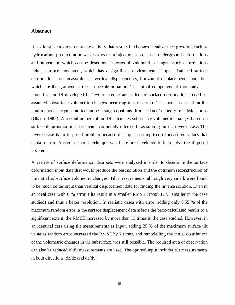
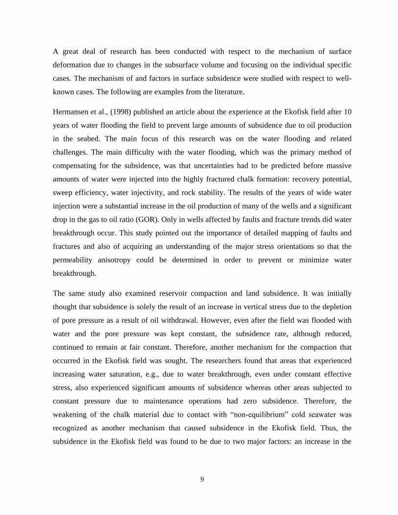
Figure 5 shows induced deformations calculated as the result of waste injection at different

depths. The results show that as the depth of the reinjection increases, meaning that volumetric

changes are happening at deeper depths, the maximum amplitude of the resulting surface

18

deformation decreases. However, as can be seen in the graph, the area affected on the surface

becomes wider as the induced volume change occurs more deeply into the subsurface.

Figure 4: Surface deformation as the result of

subsurface volume change (Rothenburg et al.,

1994).

.

Figure 5: Surface deformation as the result of

waste injection at different depths (Rothenburg

et al., 1994).

.

Dusseault et al. (2002) conducted detailed research on the data analysis of deformation

measurements for reservoir management. They pointed out that if the deformations occurring

in the reservoir due to temperature or pressure changes or withdrawal or injection of solids or

liquids are transferred linearly to the surface, a unique solution would be available for solving

for the location and magnitude of the sources of deformations that occur below the surface.

However, the presence of random error along with a limited number of data points would make

the solution non unique and ill-posed.

At the Krechba field in Algeria, Ferretti et al., (2008) carried out a study to calculate flow

properties and to identify the features that control the flow, e.g., permeability. They

investigated the possibility of using measured and observed displacement data gathered from

InSAR in order to detect the levels of carbon dioxide CO2 in the reservoir resulting from CO2

injection into the surrounding media. One characteristic of the Krechba field was that the

concentration of CO2 in the gas production was 1 % – 9 %, well above the specification for

export gas of 0.3 %. The solution that had been employed was to separate the extra CO2 from

the hydrocarbon and to reinject it into the field. The model used in the study was based on the

surface deformations caused by the reinjection CO2. Three benefits of this approach were

19

identified: the cost efficiency of using remotely gathered data, the minor effect on the results

and methodology of the heterogeneity of the mechanical properties inside the reservoir, and the

ability to solve a linear inverse problem and to calculate the flow properties.

Kroon et al. (2008) investigated a variety of processes that cause land subsidence at different

depths; the main focus was to determine the amount each of these processes affected the total

land movements observed. This research not only focused on the inverse problem resulting

from hydrocarbon extraction, but it also considered all possible parameters from both shallow

and deep depths that affected land movement, thus estimating the effect on the entire

compaction field. A Bayesian approach was used to estimate the parameters. All the

uncertainties and correlations resulting from geological and other considerations were taken

into account as prior knowledge. Quantifying variance and covariance for the prior knowledge

is therefore essential, which was accomplished using a Monte Carlo simulation.

A forward model was used to describe peat oxidation, which is a shallow compaction that

involves both poroelastic and inelastic effects. If the pre-consolidation stress is exceeded, the

compactions are irreversible. The results showed that compactions due to peat oxidation or

those that occur in clay layers, which are found at shallow depths of less than 50 m, are

transferred to the surface instantly. It was also observed that these deformations that occur at

shallow depths have a local effect on the surface: they affect areas only at the top of the

deformation points.

The second model was developed in order to study the effects of volume changes occurring

deep down in depth. They studied a case of a decrease in gas pressure due to the production in

the hydrocarbon reservoir. This decrease in pressure, which causes an increase in effective

stress, results in the compaction of the rock in the reservoir until a new equilibrium is reached.

The behaviour of the overburden was assumed to be elastic, and thus the deformation in the

subsurface was transferred almost instantly to the surface. Also because of the elastic

behaviour of the overburden, the deformation is extended to a wider range on the surface than

the length of the reservoir where the initial deformation took place. The surface deformation

field is roughly equal to the depth of the reservoir. The main purpose of the study was to focus

on the inverse case: to use the observations of surface deformation in order to determine

subsurface movements. The model was validated through tests involving a number of cases.

The results clearly indicate that neglecting deformations that occur at shallow depths, if

20

present, results in much different and incorrect data. If the inversion results based on an

observed surface deformation do not make sense or do not agree with prior knowledge, then

one or more mechanisms have not been taken into account (Kroon et al., 2008).

Land subsidence due to reservoir compaction has also been a problem in many geothermal

fields. The mechanism is generally similar regardless of the type of reservoir. Thus, it is also

helpful to study geothermal fields, the deformations that occur in them, and related research.

The Cerro Prieto geothermal field in Baja California and the Wairakei geothermal field are two

examples mentioned in the literature (Allis, 2000).

Carnec and Fabriol (1999) modeled and analysed the subsidence due to fluid withdrawal in the

Cerro Prieto geothermal field, which at the time was one of the largest liquid-dominated fields

in the world, supplying three power plants. Part of the waste fluid from the production was

reinjected into the west side of the field and part of it was evaporated in the evaporation pond.

In order to develop the model, the researchers assumed the deformation to be elastic in a half-

space from a point source. Original information was gathered in order to model the subsidence

setting. The data was gathered using images selected from InSAR data collected from 1993 to

1997. When analysed, the images revealed the presence of fringes at one corner of the area.

The fringes appeared in different combinations, which meant that they could not be present due

to atmospheric changes and effects. Moreover, their formation and altitudes indicated that they

were also not formed due to topographic effects. The studies and analysis were based on the

assumptions that the crust of the Earth is a semi-infinite ideal elastic body and that land surface

deformations are due to changes in hydrostatic pressure in a spherical source known as the

Mogi source. The best-fit model to represent the phenomena in the area and to locate the

compaction/dilation point sources at greater depths was found with trial and error. The results

indicated that areas on the surface where uplift was observed matched dilation point sources

and, therefore, reinjection areas. The depths of the Mogi sources also showed that the land

subsidence was a result of the compaction of the reservoir itself due to a drop in pore pressure

that resulted from fluid extraction. Examination of the production pattern showed that during

one period, in some local areas, production increased whereas the global withdrawal of natural

fluid was maintained at a constant level on the site. Laboratory tests conducted on sandstone

core samples taken from the wells indicated that compaction and reduction of permeability had

occurred during the production process. Subsidence was recorded both after an earthquake and

21

during an increase in the production and withdrawal of fluid (Glowacka et al., 1999). Only a

short interval was identified between events that resulted in changes in the ground water level

and the observed subsidence and compaction of sediments.

Aliss (1999) researched the Wairakei geothermal field because of its history of over 45 years of

land subsidence, with about 14−+ 0.5 m observed in the subsidence bowl due to production. The

main goal was to study the cause of the land deformation and investigate its effects. The

distribution of pressure between 1950 and 2000 as well as the mass and rate of heat flow over

time during this period were plotted, along with the history of subsidence over time during the

same period. By normalizing the subsidence graph, and comparing two benchmarks, it was

found that one area had undergone half of its total subsidence by 1963 and that the curve shows

a very low rate of subsidence in 1999, indicating that the major cause of subsidence had

dissipated and was no longer fully present. However, other areas in the eastern bore field

passed the halfway mark of their total subsidence during the mid-1970s. The subsidence in this

area caused ponding and cracking. The ponding significantly affected the environment in that

area because the roots of the trees around the ponded area were flooded, so the trees died and

fell into the expanding pond. The effects of ponding on the environment can be seen in the two

photographs in Figure 6.

Figure 6: Evolution of ponding in the Wairakei stream at the centre of the subsidence bowl. The

photograph on left was taken in 1981, and the photograph on the right was taken in 1997at almost the

same location (Allis, 2000).

As can be seen, the ecosystem in the area has been greatly affected. High rates of tilt recorded

in the area indicate high rates of extensional strain, which has resulted in the cracking of the

ground at the outer edges of the subsidence bowl. Because of erosion during heavy rainfalls,

22

these cracks became fissures up to 1 m wide. These vertical and horizontal ground strains have

also resulted in casing damage in wells in some areas.

23

3. Factors Affecting the Movement of the Ground Surface

Generally speaking, volumetric changes in the subsurface result in surface deformations. An

increase in the volume of the rock of the reservoir, due, for example, water or steam or waste

injection, which results in surface upheaval and compaction in the reservoir due to oil or liquid

withdrawal , cause land subsidence. The changes in volume that occur in the subsurface can be

caused either by natural causes such as tectonic motion, a rise in sea level (Hu et al., 2004), or

earthquakes or by human activities such as ground water withdrawal, oil and gas recovery

(petroleum industry), coal mining, sulphur and ore extraction, other mining activities,

underground excavations to create tunnels and caverns, and steam or waste reinjection (Nagel,

2001). These changes in the subsurface can occur at shallow depths due to construction work,

such as the building of foundations and tunnels; peat oxidation; the compaction of clay layers;

ground water withdrawal. They can also occur at much greater depths because of earthquakes,

hydrocarbon production, salt production, or waste reinjection. A change in volume at both

shallow and deeper depths affects the surface and causes deformations. It has been proven that

a surface deformation field created as the result of a point source placed at depth d beneath the

surface with a volume change of ΔV can be described approximately as an area with a radius d

above the center of the volume change (Kroon et al., 2008) (Figure 7).

Figure 7: The approximate deformation field as a result of a point source of volume change at depth d.

When discontinuities in volume change are considered as sources of subsurface deformations

for modeling purposes, it should be remembered that the principles of the physical occurrence

Approximate deformation field with radius d on the surface

Point source of volume change at depth d

24

of compaction or swelling and resulting land deformation are generally the same for all

reservoirs, hydrocarbon reservoirs, water reservoirs, geysers, geothermal fields, waste injection

fields, etc., regardless of the type of material withdrawn or injected. The major difference lies

in the varying geometry, geological settings, and material properties that differ for specific

cases and specific reservoirs and that require the application of different models (Gambolati,

1975).

In the oil and gas industry, the causes of surface deformations are usually reservoir compaction

or expansion due to fluid withdrawal or reinjection. Thus, the changes in volume that occur in

the reservoir depend on many internal factors, such as the properties of the rock in the

reservoir, the history of its formation, its geometry, and external factors, such as external loads

and the overburden material. The geometry of the reservoir has a sizable impact on the way it

will react upon recovery and during injection and has a significant effect on induced

deformations that can be monitored on the surface. The most important factors in the geometry

of a reservoir are its depth and width, and the ratio between them is critical. If this ratio is

larger than 1, meaning that the width is greater than its depth, most of the vertical deformation

in the reservoirs is transferred linearly to the surface, and the surface deformation is a function

of the change in the reservoir’s height (∆𝐻).

Deformations that occur at significant depths and inside the reservoir are transferred to the

surface through the overburden material. The behaviour and properties of the overburden

material therefore have a substantial impact on the deformations that occur and can be

observed on the surface. Although reservoir deformations may be plastic and irreversible

locally, the behaviour of the overburden material also must be elastic in order for its behaviour

to be modeled and a solution produced (Dusseault et al., 2002). According to d’Alembert’s

principle, when a 3D setting of a medium is modelled, a plastic strain at a point can be

translated into an elastic strain at a very small distance from the initial source. With respect to

the behaviour of overburden material over oil reservoirs, since the strains induced in the

overburden are very small, in the order of (휀 < 10−4), even in cases where huge vertical

deformations are observed on the surface, it is correct to assume that the overburden acts

elastically in most cases (Dusseault et al., 2002).

25

Land deformation due to changes in the volume of the reservoir can be observed as vertical,

horizontal, and tilts. However, according to site observations and past studies it has been

determined that the maximum values of displacement due to reservoir compaction occur in a

vertical direction (Bruno et al., 1990) because of the geometry of reservoirs. The width of a

reservoir is far greater than its thickness, which results in vertical surface deformations being

much larger than any horizontal movements induced on the surface (Dusseault et al., 2002).

Over oil and gas reservoirs, the vertical surface movements have been found to be three to five

times larger than the horizontal displacements (Bruno et al., 1990). However, the thousands of

well-casing failures observed and recorded in oil fields are not the result of vertical

deformation, but are due mostly to shear and bending deformations. Thus, although horizontal

displacements and tilts may be small in magnitude, the damage they cause is not insignificant,

and they should therefore be studied seriously as well. Tilts also provide important information

about the surface deformation field, and their use as input data for investigating changes in the

volume of a reservoir is therefore the focus of this thesis.

3.1 Geological terminology

3.1.1 Definition of a reservoir

A reservoir is a formation of one or more subsurface rock formations that contain a natural

accumulation of liquid and or gaseous hydrocarbons. A reservoir rock formation itself is

porous and permeable. The pores should interconnect to let fluids migrate through the rock and

the rock itself should be permeable to have the ability to allow the flow of the fluid through it

(Cosse, 1993; Amyx et al., 1960; Calhoun, 1917). This characteristic of the reservoir rock or

the subsurface material is the reason that the reservoir or soil compacts because of an increase

in effective stress.

How the subsurface reacts under loading, production, and reinjection activities depends strictly

on several groups of factors: the characteristics of the subsurface material, the structural

features of the reservoir, the characteristics and properties of the reservoir fluid, the pressures

present or induced inside the subsurface, the temperatures inside the reservoir, and the

operating conditions implicit in the media (Calhoun,1917).

26

3.1.2 Reservoir materials

One method of classifying the material in a reservoir is to describe it based on the grain types

and the type of soil particles that form the reservoir rock.

The rock in a reservoir is composed mainly of sedimentary materials, generally sandstones or

limestones. Sandstones and or carbonates, which are sedimentary rocks, comprise 99% of

reservoirs (Cosse, 1993; Amyx, 1960).

The best way to describe and study a reservoir and its properties and behaviour under loading,

production, or reinjection is to describe the reservoir in terms of measurable engineering

quantities, the most useful of which are porosity and permeability (Calhoun, 1917). These two

factors are often used to calculate and predict the deformations and compactions that occur

inside and above reservoirs.

A soil sample is composed of all three phases of materials: solid (grain particles), liquid

(water), and air. Porosity is defined as the ratio of the volume of voids (volume of air + volume

of water) in a soil sample to the total volume of the soil sample (Das, 2006):

𝑛 =𝑉𝜐

𝑉𝑡 (3.1)

A high porosity indicates a higher volume of voids in a constant volume of soil sample and

such a soil would undergo a higher amount of compaction under a load or an increase in the

effective stress.

A soil or rock formation is permeable due to the existence of interconnected voids or fractures

that provide a path for water to penetrate and move through (Das, 2006).

3.2 Mechanical properties of a reservoir and the compaction subsidence

mechanism that occurs due to oil withdrawal

The weight of sediments and any other material that is placed on the soil over a reservoir,

otherwise referred to as external loads, is supported by both the rock matrix of the reservoir

and the fluid within the rock pore space (Hermansen et al., 2000). The total stress is thus the

result of the summation of the effective stress, i.e., the stress carried by the soil skeleton, and

the pore pressure, which is the weight carried by the water inside the porous medium.

27

𝜎𝑣 = 𝜎 ′ + 𝑢 (3.2)

Thus, when fluid is withdrawn from inside the reservoir, the pore pressure drops. If the total

stress remains constant, the load that was initially supported by the fluid is now transferred to

the solid matrix, and the effective stress increases. Now tolerating a greater load than before,

the rock formation is compacted due to the additional stress. The increase in the effective stress

can be caused either by an increase in the external loads, such as the addition of facilities and

equipment for oil excavation, or by a decrease in the pore pressure inside the soil or rock

matrix. A decrease in pore pressure can be due to a decrease in the level of the underground

water table in the soil layers or to oil or fluid withdrawal from inside the reservoir. An increase

in pore pressure is the result of an increase in the level of the underground water table or of

reinjection and water flooding inside reservoirs. Thus, the equilibrium present in the soil prior

to any change no longer exists after the change in pore pressure.

Rock or layers of soil react to loading or to an increase in the effective stress, and to unloading

or to a decrease in the effective stress differently based on the history of the soil. The

consolidation type of the material, which is basically an indication of the load history of the

material, is thus of great importance in studying and understanding the behaviour of the

material under loading or unloading and also in defining specific qualities of the material, such

as compressibility. By performing the oedometer test on a sample of the soil obtained at the

depth of study, geotechnical engineers in a laboratory can produce a very important graph: the

void ratio plotted against the log of the effective stress (Figure 8). From this graph, the

maximum effective stress that has been tolerated by the soil at that specific depth can be

calculated. When the effective stress present at the site is compared with this maximum

effective stress from the graph, a current effective stress (𝜎0′ ) that is lower than the maximum

effective stress (𝜎𝑐′ ) indicates that the soil has tolerated higher loads during its formation than

those present at the time. This soil is referred to as pre-consolidated or over-consolidated. If the

effective stress present at the time is larger or equal to the maximum effective stress from the

graph, the soil or material is weak and is expected to undergo more deformations and more

compaction due to an increase in the effective stress. This soil is referred to as normally

consolidated soil.

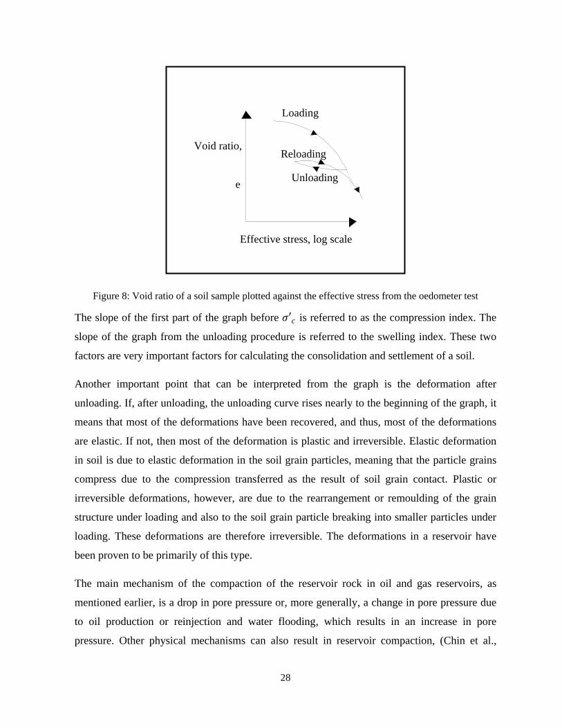
28

Figure 8: Void ratio of a soil sample plotted against the effective stress from the oedometer test

The slope of the first part of the graph before 𝜎′𝑐 is referred to as the compression index. The

slope of the graph from the unloading procedure is referred to the swelling index. These two

factors are very important factors for calculating the consolidation and settlement of a soil.

Another important point that can be interpreted from the graph is the deformation after

unloading. If, after unloading, the unloading curve rises nearly to the beginning of the graph, it

means that most of the deformations have been recovered, and thus, most of the deformations

are elastic. If not, then most of the deformation is plastic and irreversible. Elastic deformation

in soil is due to elastic deformation in the soil grain particles, meaning that the particle grains

compress due to the compression transferred as the result of soil grain contact. Plastic or

irreversible deformations, however, are due to the rearrangement or remoulding of the grain

structure under loading and also to the soil grain particle breaking into smaller particles under

loading. These deformations are therefore irreversible. The deformations in a reservoir have

been proven to be primarily of this type.

The main mechanism of the compaction of the reservoir rock in oil and gas reservoirs, as

mentioned earlier, is a drop in pore pressure or, more generally, a change in pore pressure due

to oil production or reinjection and water flooding, which results in an increase in pore

pressure. Other physical mechanisms can also result in reservoir compaction, (Chin et al.,

Effective stress, log scale

Unloading

Reloading

Loading

Void ratio,

e

29

1993) some of which relate to the reservoir rock and others to the properties and behaviour of

the overburden. The following are some of the mechanisms that result in the compaction of a

reservoir:

Pore pressure drops due to oil production.

Shear induces compaction. Of course, shear does not itself result directly in

compaction. However, the stress state due to shear concentrations causes the matrix

blocks to displace slightly with respect to one another, these non-equal movements

result in concentrated zones of stress that may produce fractures, and thus more

displacements under pore pressure changes occur due to this weaker formation (Chin et

al., 1993).

The weakening of some types of reservoir rock material, such as chalk, due to contact

with non-equilibrium cold seawater, e.g., in the Ekofisk field (Hermansen et al., 2000).

Mechanical properties of the overburden material can cause compaction.

These mechanisms cause deformations in the subsurface due to changes in fluid pressure, such

as water flooding or oil production. However, in other cases, such as waste injection, when a

material is forced into the subsurface, these mechanisms do not apply. The deformations are a

result of forcing an external material such as waste into the subsurface area, which then results

in surface deformations.

3.2.1 Parameters affecting reservoir compaction

In nature, compaction depends on the overburden load, the amount of this load that is

transferred to the reservoir, the tectonic loads applied to the formation, and the strength of the

rock. Tectonic movements, although very small, slowly break the contacts between grains in

different areas, thus resulting in the rearrangement and compaction of the grains even without

any additional load (Gurevich et al., 1993). Periodic temperature changes cause the same

damage and rearrangement of grain particles, thus creating compaction. Generally,

disregarding thermal and chemical effects such as dissolution, reservoir compaction can be

considered a function of three parameters: increases in the effective stress, the thickness of the

reservoir, and the compressibility of the reservoir rock (Nagel, 2001).

30

3.2.1.1 Increases in the effective stress

Originally, prior to the production and withdrawal of oil, the reservoir rock and the overburden

are both in equilibrium conditions. The rock has been consolidated and compacted by the

effective stress present due to the overburden material and the loads placed on it. As oil

production starts, the pore pressure drops because of fluid withdrawal. The total stress remains

constant, so the effective stress increases. As the effective stress increases, the pressure on the

reservoir rock matrix increases, causing it to compact. The reservoir rock compacts up to the

point at which the matrix re-establishes new equilibrium states (Nagel, 2001).

If the compaction of the reservoir rock is the result of an increase in the effective stress due to

fluid withdrawal, it can be controlled by controlling the pressure of the pore water (Nagel,

2001), either by managing the production rate or by reinjecting water into the reservoir to

compensate for the loss in pressure. The principle is that after fluid withdrawal has stopped, if

the pore pressure has remained constant or has increased, e.g., because of injection, then some

part of the subsidence is recoverable and even a measure of uplift on the surface can be

observed in some cases. This phenomenon is known to be due to the relaxation of the

elastically compressed overburden materials after the pore pressure has been increased and is

commonly known as elastic rebound. A good example of elastic rebound in the literature is the

extensive research on reinjection experiments carried out at the Wilmington oilfield in

California (Chen et al., 2007).

3.2.1.2 Thickness of the reservoir

Unlike changes in effective stress, reservoir thickness is an intrinsic characteristic of the

reservoir that cannot be changed (Nagel, 2001). Most well-known compacting reservoirs are

relatively thick, with measurements greater than 100 m. Generally, the greater the thickness of

a reservoir, the more compaction is expected to undergo. Thus, the thickness of a reservoir has

a direct relationship to its compaction (Nagel, 2001). In Table 1 lists the thickness and other

properties of the most common oil reservoirs.

31

Table 1: Properties of common subsiding oil reservoirs (Nagel, 2001).

3.2.1.3 Compressibilityof the reservoir rock

The compressibility of the reservoir rock is another factor that affects its compaction. Like

thickness, compressibility is an intrinsic characteristic of the reservoir, but these two

parameters work in opposition to each other, meaning that a thin but highly compressible

reservoir and a thick but less compressible reservoir may have the same amount of compaction

under the same pore pressure drop and similar conditions. Although compressibility is an

intrinsic characterization of the reservoir, unlike thickness, in some cases, it can be altered.

Thermal or geochemical effects can change compressibility, and it has been proven that

changes in water saturation also lead to significant changes in the compressibility of a reservoir

(Nagel, 2001).

Of the three parameters that affect the compaction of a reservoir, compressibility is the hardest

to measure accurately. Compressibility is itself a function of other parameters, such as the

mineral composition of the rock matrix, the degree of mineral decomposition or alteration, the

cementation and porosity of the rock, and the degree of sorting. Well sorted refers a soil

formation in which the sediment sizes are similar whereas poor sorted refers to mixed sediment

sizes. Of these factors, porosity is the critical parameter that defines the compressibility of a

rock or soil. Table 1 shows that the majority of highly compactable reservoirs have a porosity

level greater than 30 %.

According to Bruno (1990), who conducted detailed research with respect to the

compressibility of reservoir rock, rock compressibility itself depends on two important factors:

Material pore volume compressibility 𝐶𝑝

Bulk compressibility 𝐶𝑏

32

These two factors are defined as follows:

𝐶𝑝 =1

𝑉𝑝∗

∆𝑉𝑝

∆𝑃𝑝 (3.3)

𝐶𝑏 =1

𝑉𝑏∗

∆𝑉𝑝

∆𝑃𝑝 (3.4)

where 𝑉𝑝= pore volume

𝑉𝑏= bulk volume

𝑃𝑝= pore pressure

𝐶𝑝 and 𝐶𝑏 are defined as the change in pore volume and bulk volume, respectively, with

respect to pore pressure change, ∆𝑃𝑝 at a constant confining pressure. These two factors are

well defined in theory, but in some cases, such as in diatomite reservoirs, where the

deformations are inelastic at almost all stress levels, these factors can be defined only

empirically through laboratory measurements.

3.3 Methods of monitoring reservoir compaction (subsurface monitoring)

The casing collar locator log method is one of the earliest methods of monitoring reservoir

compaction. Using this method, the change in the distance between casing collars is measured

in order to determine and monitor the compaction of a reservoir. The accuracy of the data

gained from this method is 0.012−+ m per casing joint. This method is very dependent on the

coupling of the reservoir rock and the casing, and the results are therefore questionable in the

majority of cases (Nagel, 2001).

Compaction monitoring with radioactive bullets shot into the formation is another method

that is not sensitive to the interaction between the casing and the reservoir. Radioactive bullets

are shot into the formation at regular intervals. After statistically analysing the data and with

the use of accelerometer corrections to account for errors due to any irregular movements of

the tool, changes in the distance between two bullets can be measured even up to 1 cm. If the

bullets are shot into the overburden, it would be possible to obtain the ratio between the

compaction of the reservoir and the surface subsidence that results from the transfer of the

subsurface compaction.

33

This method also has limitations. If the bullet does not penetrate to the desired extent, the

results are neither accurate nor useful (Nagel, 2001).

Monitoring porosity over time is an indirect way of monitoring the compaction of a reservoir.

Since compaction results in a decrease in pore volume, compaction can be monitored by

logging the porosity. Changes in the porosity in the reservoir rock can then be linked to the

compression of the reservoir by comparing the results to the behaviour measured through

laboratory testing and changes in the porosity due, for example, to a given strain in the uniaxial

test. The results produced by this method can be inaccurate because of the heterogeneity of the

distribution of the porosity inside the entire reservoir and also because of the limitations of the

accuracy of porosity logging (Nagel, 2001).

Micro seismic surveys and the use of 4D seismic technology are other methods of monitoring

the compaction of a reservoir. These methods are limited because of the presence of gas in the

overburden material, the effects of changes in the degree of water saturation on rock velocity,

and their level of accuracy (Nagel, 2001).

Reservoir compaction monitoring is carried out in order to determine the conditions and

changes inside the reservoir. This data is needed in order to determine and predict the motion

of the ground and the surface subsidence as a result of oil production. However, as can be seen,

these procedures are time consuming, and the results can be inaccurate if the set-up is not

precise. Deformations induced in the subsurface due to injections, e.g., waste injection are not

easy to monitor, which explains why the inverse case has become of great interest to

researchers.

3.4 Overburden material and the degree to which subsurface compaction is

transferred to the surface

The degree to which the induced subsurface deformations are transferred to the surface and

thus the amount and shape of the resulting surface deformation are dependent on the following

factors: the geometry and areal extent of the reservoir, the depth of the reservoir burial, the

stiffness properties of the material surrounding the pressure-depleted zone (Bruno, 1990), and

the mechanical properties of the overburden material (Chin et al., 1993).

34

Deformations in the subsurface occur primarily in the central portion of the reservoir, usually

where the porosity is the highest. Once the reservoir deforms, the overburden on top deforms

as well. If a compaction zone is induced in the subsurface, the overburden moves downward as

well. However, it also resists the deformation and attempts to remain rigid over the reservoir,

flexing down over the crest of the reservoir but pinned on the exterior of the flanks of the

reservoir. Thus, a portion of the load which was supported by the centre of the reservoir rock is

transferred to the regions at the edges. This phenomenon is referred to as the arch effect. When

the load is transferred to the edges, less of the load is supported by the reservoir rock, which

results in less deformation. The effect of the overburden resisting deformation depends on the

mechanical properties of the overburden, and the arching effect results in the development of

shear stresses. The maximum values of these stresses are found primarily on the edges, where

transition occurs between layers of material. If the shear stresses become large enough that the

overburden loses its ability to resist deformation, the arching is no longer effective and the load

transfer characteristics become less effective as well (Chin et al., 1993).

The presence of vertical tensile strains and elongations above a compacting reservoir is

evidence of the bridging effect and indicates that all of the overburden weight has not been

fully transmitted to the reservoir. The result is that the reservoir compacts much faster than the

overlying material and layers (Gurevich et al., 1993).

3.5 Surface deformation monitoring

The deformations induced in the subsurface are transferred to the surface through the

overburden material, and the surface deforms as a result. If the reservoir is horizontal and

homogeneous, the displacement contour observed on the surface appears as displaced points

positioned around the centre of the volume change (injection or production wells) (Vasco et al.,

2002). However, in most cases, a fault zone is inside or close to the reservoir and causes

skewing of the distribution of the volume change and the resulting surface deformations. Thus,

it can be seen that observing only the pattern of the surface deformations can provide an idea of

the distribution of the changes in volume inside the reservoir, and since the distribution of the

changes in volume is related mainly to reservoir permeability and compressibility, from the

discontinuities found in the distribution of the changes in volume in the reservoir, these two

parameters can be solved for as well (Vasco et al., 2002). Surface monitoring is also an

35

effective method of checking for validation of the models used to predict future subsidence or

upheaval and can thus be used to solve the direct problem.

Monitoring surface deformations is therefore a very important part of the production operation.

The most common techniques for measuring and monitoring deformations in the petroleum

industry, steam reinjection projects, and waste reinjection are as follows:

3.5.1 Global positioning system (GPS)

Using this method, data can be collected periodically, and the elevation of each given

observation point in the field can be determined with centimetre-level accuracy. Global

positioning satellites are used to monitor the vertical and horizontal movement of receiver

stations, each of which must contain a receiver and a data collection system.

3.5.2 Interferometric synthetic aperture radar (InSAR)

This method also uses satellites that can map and document surface displacements at both a

large and small scale but with less accuracy than GPS. In this method, the changes in phase

between satellite radar images are used to determine changes in elevation. This method is used

for mapping topography, for monitoring and recording displacements induced by earthquakes

and displacements in magnetic fields, for producing images of ice dynamics, and for

monitoring subsidence induced by mining and geothermal production (Nagel, 2001; Du et al.,

2001; Vasco et al., 2002).

3.5.3 Tilt meter monitoring

Tilt meter monitoring is currently one of the most popular methods of observing and

monitoring land subsidence, especially in the oil and gas industry. This technology uses highly

precise levels placed near the surface in order to measure deformations that occur due to field

operations such as oil production, fluid withdrawal, fluid injection, and hydraulic fracturing.

Tilt meters measure what are called tilts, which are displacement gradients.

The common use of the tilt meter has resulted from its advantages over other methods: its very

high precision and ability to detect motion in the order of 10−5 m and its continuous data

collection capability that permits deformations due to production, injection, or any other type

of field operations to be closely monitored.

36

3.5.4 Levelling and distance survey data

The use of levelling and distance survey data is one of the oldest methods of monitoring

subsidence. A network of stations is established in the area, and motion in each is monitored

over time. This method is costly and time consuming and its application is usually limited to

onshore sites (Ferretti et al., 2008; Nagel, 2001).

The usual purpose of monitoring is to solve the inverse case, which requires a large number of

observation points. Obtaining data by means of one of the above methods is much less costly

and faster than having to drill deep wells into the reservoir and using pressure gauges and

sensors to record changes in pressure. It is for this reason that solving the inverse case is of

interest.

The data recorded from surface monitoring is used for the following purposes:

monitoring of hydraulic fracturing

monitoring of fluid migration in volcanic areas

steam injection

well testing

petroleum production

monitoring of waste reinjection and fracture and the resulting subsurface deformation

37

4. Mathematical Approach

4.1 Direct case

The direct case to be solved involves the calculation or prediction of surface deformations due

to subsurface movements, based on measured reservoir compaction and changes in volume in

the reservoir rock or in the subsurface, using data gathered from the methods mentioned in

section 3.3 or using the distribution of changes in volume assumed to be occurring within the

reservoir to further predict the induced surface movements. All calculations in this thesis are

based on Okada’s formulas (Okada, 1985). Okada’s solution models concentrated on the

expansion or compaction that occurs in one direction, which is certainly not an exact

representation of what is actually taking place but is a very good approximation. The approach

used in previous models for similar inverse cases was to use the nucleus of strain approach

(e.g., Bilak, 1989). Nucleus of strain is a model that describes deformation as expansion or

compaction points being deformed into the space of the subsurface in all directions. Figure 9

shows a point source representing expansion in volume in the subsurface using the nucleus of

strain approach.

Figure 9: Change in volume modeled as a point of expansion in the subsurface: nucleus of strain

approach.

Since the reservoir elements are much smaller than the geometry of the reservoir and its depth,

it is correct to assume that the volume changes that occur in each reservoir element can be

remodelled as point sources. These point sources that represent volume changes in each

38

element and are assumed to be at the centre of each cubic element are referred to as nucleus of

strain points (Figure 10).

Figure 10: Nucleus of strain points in reservoir elements.

The concept of nucleus of strain was first introduced by Geertsma (1973) in the field of

continuum mechanics. According to this concept, it is assumed that the volumetric strain at an

element caused by local reduction or a change in pore pressure can be treated as a compression

point, or, an expansion point, in the centre of an elastic half-space. This assumption would

result in deformations induced in the free space. Thus the deformation at a given point on the

surface is the result of the contribution of these compression or dilation nucleolus of strain

points in the reservoir elements using the nucleus of strain approach.

Modelling an actual deformation in all directions using Okada’s method requires the addition

of three Okada solutions in three directions. The results would of course differ slightly from

those produced by the nucleus of strain approach which represents deformations as a series of

nucleus of strains, and are integrated over the reservoir.

It is difficult to say which approach is closest to reality; however, in the reservoirs that are the

main focus of this research, the thickness is much smaller than depth or width so the majority

of deformations occur vertically. Because deformations induced in these cases are mostly one

dimensional, displacement discontinuity provides a better model for these applications.

A number of assumptions were made in modeling and solving for the direct case. The media

was assumed to be an isotropic homogenous semi-infinite medium (Okada, 1985) and the only

39

source of subsurface volumetric change was assumed to be that of the reservoir. Since the

length of a reservoir is normally much larger than its thickness, for the purposes of this thesis,

the shape of the reservoir was assumed to be a thin rectangular plate (Figure 11).

Figure 11: Shape of the reservoir assumed for modeling.

Although many factors that affect the land and surface deformations in reality were neglected,

such as the curvature of the Earth, the surface topography, crustal layering, inhomogeneity or

vertical layering, and angled layered medium, the results are still acceptable. Previous studies

have shown that the curvature of the Earth can be negligible in events happening at shallow

depths and at distances of less than 20 degrees. However, vertical layering has a significant

effect on deformations and the results of modeling (Okada, 1985). Despite this factor and the

many others that can be involved in an actual modeling of the Earth, the assumption of a

simple isotropic homogenous half-space was used for this study. The assumptions made can be

considered acceptable because the theoretical models based on these assumptions have been

proven to be good approximations of actual cases (Okada, 1985).

The subsurface source that causes induced surface deformations was modeled as a finite

rectangular source (Okada, 1985).

Finite rectangular source

The source of subsurface deformation can be described as a finite rectangular source that

causes deformations. To model the deformations, the reservoir was divided into smaller

rectangular elements. Each element was considered to undergo a change in volume due to

40

activities such as oil production, steam reinjection, and waste injection. The source resulting in

subsurface deformation was thus considered to be a finite rectangular source.

Based on Figure 12 from Okada (1985), the total force is the source of deformation. Thus the

volumetric deformations resulting from the total force can be described as the combination of

three forces or changes in dimension in three directions, as follows:

x direction: the change would be along the x axis in the Cartesian coordinate system,

y direction: the change would be along the y axis in the Cartesian coordinate system.

z direction: the change would be along the z axis in the Cartesian coordinate system.

Figure 12: A general form of reservoir plate with a dip angle of 𝛿, a length of L, a width of W, a depth

of –d, and an Azimuth of 0ᵒ (Okada, 1985).

As can be seen in Figure 12, the elastic medium occupies the area of z<=0 in the selected

coordinate system. This research was focused on the dislocations caused by the finite

rectangular source rather than on the force itself. As mentioned above, the dislocation can be

described as the combination of the dislocations in the three major directions in the Cartesian

system. 𝑈1, the vector in the x direction corresponds to strike-slip; 𝑈2, which is the vector of

dislocation parallel to the y axis, is referred to as dip-slip; and 𝑈3, which is the vector of

dislocation parallel to the z axis, is referred to as the tensile component of a general

41

dislocation. The fault, which in this case represents the reservoir, or to be more precise, a

rectangular element of the reservoir with a length L and a width W, is modeled for a general

case with an angle of rotation of 𝛿 from the XY plane (dip angle) and an azimuth (the rotation

angle of the reservoir from the X axis).

Due to the subsurface dislocations, which are assumed to be the result of a rectangular finite

force, the induced surface deformations occur on the surface in all three directions (x, y, and z).

The first two induced surface deformations are referred to as horizontal deformations, and the

third is called the vertical displacement or deformation. Based on Okada (1985), the resulting

deformations on the surface can be calculated using the following formulas:

Displacements

For strike-slip (4.2)

𝑢𝑥 = −

𝑈1

2𝜋

휁𝑞

𝑅 𝑅 + 휂 + 𝑡𝑎𝑛−1

휁휂

𝑞𝑅+ 𝐼1𝑠𝑖𝑛𝛿 ||

𝑢𝑦 = −𝑈1

2𝜋

Ϋ𝑞

𝑅 𝑅 + 휂 +

𝑞𝑐𝑜𝑠𝛿

𝑅 + 휂+ 𝐼2𝑠𝑖𝑛𝛿 ||

𝑢𝑧 = −𝑈1

2𝜋

Ϊ𝑞

𝑅 𝑅 + 휂 +

𝑞𝑠𝑖𝑛𝛿

𝑅 + 휂+ 𝐼4𝑠𝑖𝑛𝛿 ||

where

𝑢𝑥 = surface displacement in the x direction due to the strike-slip dislocation 𝑈1

𝑢𝑦 = surface displacement in the y direction due to the strike-slip dislocation 𝑈1

𝑢𝑧 = surface displacement in the z direction due to the strike-slip dislocation 𝑈1

휁 = 𝑋𝐿 − 0.5𝑓𝑙

휂 = 𝑌𝐿. cos 𝑑𝑖𝑝 + 𝑑. sin 𝑑𝑖𝑝

where

𝑋𝐿 = 𝐷𝑥. cos 𝑑𝑖𝑝 + 𝐷𝑦. sin 𝑑𝑖𝑝

42

𝑌𝐿 = −𝐷𝑥. sin 𝑑𝑖𝑝 + 𝐷𝑦. cos 𝑑𝑖𝑝

𝐷𝑥 = 𝑥0 − 𝑥𝑓

𝐷𝑦 = 𝑦0 − 𝑦𝑓

Where

𝑥0& 𝑦0 = 𝑐𝑜𝑜𝑟𝑑𝑖𝑛𝑎𝑡𝑒𝑠 𝑜𝑓 𝑡𝑕𝑒 𝑜𝑏𝑠𝑒𝑟𝑣𝑎𝑡𝑖𝑜𝑛 𝑝𝑜𝑖𝑛𝑡

𝑥𝑓& 𝑦𝑓 = 𝑐𝑜𝑜𝑟𝑑𝑖𝑛𝑎𝑡𝑒𝑠 𝑜𝑓 𝑡𝑕𝑒 𝑟𝑒𝑠𝑒𝑟𝑣𝑜𝑖𝑟 𝑒𝑙𝑒𝑚𝑒𝑛𝑡

For dip-slip (4.3)

𝑢𝑥 = −

𝑈2

2𝜋 𝑞

𝑅− 𝐼3𝑠𝑖𝑛𝛿𝑐𝑜𝑠𝛿 ||

𝑢𝑦 = −𝑈2

2𝜋

Ϋ𝑞

𝑅 𝑅 + 휁 + 𝑐𝑜𝑠𝛿𝑡𝑎𝑛−1

휁휂

𝑞𝑅− 𝐼1𝑠𝑖𝑛𝛿𝑐𝑜𝑠𝛿 ||

𝑢𝑧 = −𝑈2

2𝜋

Ϊ𝑞

𝑅 𝑅 + 휁 + 𝑠𝑖𝑛𝛿𝑡𝑎𝑛−1

휁휂

𝑞𝑅− 𝐼5𝑠𝑖𝑛𝛿𝑐𝑜𝑠𝛿 ||

where

𝑢𝑥 = surface displacement in the x direction due to the dip-slip dislocation 𝑈2

𝑢𝑦 = surface displacement in the y direction due to the dip-slip dislocation 𝑈2

𝑢𝑧 = surface displacement in the z direction due to the dip-slip dislocation 𝑈2

For tensile fault (4.4)

𝑢𝑥 = −

𝑈3

2𝜋

𝑞2

𝑅(𝑅 + 휂)− 𝐼3𝑠𝑖𝑛𝛿2 ||

𝑢𝑦 = −𝑈3

2𝜋

−Ϊ𝑞

𝑅 𝑅 + 휁 − 𝑠𝑖𝑛𝛿{

휁𝑞

𝑅 𝑅 + 휂 − 𝑡𝑎𝑛−1

휁휂

𝑞𝑅} − 𝐼1𝑠𝑖𝑛𝛿2 ||

𝑢𝑧 = −𝑈3

2𝜋

Ϋ𝑞

𝑅 𝑅 + 휁 + 𝑐𝑜𝑠𝛿{

휁𝑞

𝑅 𝑅 + 휂 − 𝑡𝑎𝑛−1

휁휂

𝑞𝑅} − 𝐼5𝑠𝑖𝑛𝛿2 ||

43

In the above formulas, (4.5)

𝐼1 =𝜇

𝜇 + 𝜆

−1

𝑐𝑜𝑠𝛿

휁

𝑅 + Ϊ −

𝑠𝑖𝑛𝛿

𝑐𝑜𝑠𝛿𝐼5

𝐼2 =𝜇

𝜇 + 𝜆 ln(𝑅 + 휂) − 𝐼3

𝐼3 =𝜇

𝜇 + 𝜆

1

𝑐𝑜𝑠𝛿

Ϋ

𝑅 + Ϊ− ln(𝑅 + 휂) +

𝑠𝑖𝑛𝛿

𝑐𝑜𝑠𝛿𝐼4

𝐼4 =𝜇

𝜇 + 𝜆

1

𝑐𝑜𝑠𝛿 ln(𝑅 + Ϊ) − 𝑠𝑖𝑛𝛿ln(𝑅 + 휂)

𝐼5 =𝜇

𝜇 + 𝜆

2

𝑐𝑜𝑠𝛿𝑡𝑎𝑛−1

휂 𝑋 + 𝑞𝑐𝑜𝑠𝛿 + 𝑋 𝑅 + 𝑋 𝑠𝑖𝑛𝛿

휁 𝑅 + 𝑋 𝑐𝑜𝑠𝛿

where

μ and λ are Lame’s constants

μ = shear modulus = ∆𝐹/𝐴

∆𝐿/𝐿 where

𝐹 = shear stress

𝐴 = area

𝛥𝐿 = distance between shearing planes

𝐿 = shear distance

λ = k-2/3*μ where

k = bulk modulus

If 𝑐𝑜𝑠𝛿 = 0, (4.6)

𝐼1 = −𝜇

2(𝜇 + 𝜆)

휁𝑞

(𝑅 + Ϊ)2

𝐼3 =𝜇

2(𝜇 + 𝜆)

휂

𝑅 + Ϊ+

Ϋ𝑞

(𝑅 + Ϊ)2− ln(𝑅 + 휂)

44

𝐼4 = −𝜇

𝜇 + 𝜆

𝑞

𝑅 + Ϊ

𝐼5 = −𝜇

𝜇 + 𝜆

휁𝑠𝑖𝑛𝛿

𝑅 + Ϊ

(4.7)

𝑝 = 𝑦. 𝑐𝑜𝑠𝛿 + 𝑑. 𝑠𝑖𝑛𝛿

𝑞 = 𝑦. 𝑠𝑖𝑛𝛿 − 𝑑. 𝑐𝑜𝑠𝛿

Ϋ = 휂. 𝑐𝑜𝑠𝛿 + 𝑞. 𝑠𝑖𝑛𝛿

Ϊ = 휂. 𝑠𝑖𝑛𝛿 − 𝑞. 𝑐𝑜𝑠𝛿

𝑅2 = 휁2 + 휂2 + 𝑞2 = 휁2 + Ϋ2 + Ϊ2

𝑋2 = 휁2 + 𝑞2

Strains


𝜕𝑢𝑥0

𝜕𝑥=

𝑈1

2𝜋 휁2𝑞𝐴휂 − 𝐽1𝑠𝑖𝑛𝛿 ||

𝜕𝑢𝑥0

𝜕𝑦=

𝑈1

2𝜋

휁3Ϊ

𝑅3(휂2 + 𝑞2)− (휁3𝐴휂 + 𝐽2)𝑠𝑖𝑛𝛿 ||

𝜕𝑢𝑦0

𝜕𝑥=

𝑈1

2𝜋 휁𝑞

𝑅3𝑐𝑜𝑠𝛿 + (휁𝑞2𝐴휂 − 𝐽2)𝑠𝑖𝑛𝛿 ||

𝜕𝑢𝑦2

𝜕𝑦=

𝑈1

2𝜋 Ϋ𝑞

𝑅3𝑐𝑜𝑠𝛿 + { 𝑞3𝐴휂 𝑠𝑖𝑛𝛿 −

2𝑞𝑠𝑖𝑛𝛿

𝑅 𝑅 + 휂 −

휁2 + 휂2

𝑅3𝑐𝑜𝑠𝛿 − 𝐽4}𝑠𝑖𝑛𝛿 ||

For dip-slip (4.9)

𝜕𝑢𝑥0

𝜕𝑥=

𝑈2

2𝜋 휁𝑞

𝑅3+ 𝐽3𝑠𝑖𝑛𝛿𝑐𝑜𝑠𝛿 ||

45

𝜕𝑢𝑥0

𝜕𝑦=

𝑈2

2𝜋 𝑞Ϋ

𝑅3−

𝑠𝑖𝑛𝛿

𝑅+ 𝐽1 𝑠𝑖𝑛𝛿𝑐𝑜𝑠𝛿 ||

𝜕𝑢𝑦0

𝜕𝑥=

𝑈2

2𝜋 Ϋ𝑞

𝑅3+


𝑅 𝑅 + 휂 + 𝐽1𝑐𝑜𝑠𝛿𝑠𝑖𝑛𝛿 ||

𝜕𝑢𝑦0

𝜕𝑦=

𝑈2

2𝜋 Ϋ2𝑞𝐴휁 −

2Ϋ

𝑅 𝑅 + 휁 +

휁𝑐𝑜𝑠𝛿

𝑅 𝑅 + 휂 𝑠𝑖𝑛𝛿 + 𝐽2𝑠𝑖𝑛𝛿𝑐𝑜𝑠𝛿 ||


𝜕𝑢𝑥

𝜕𝑥= −

𝑈3

2𝜋 𝑞2휁𝐴휂 + 𝐽3𝑠𝑖𝑛

2𝛿 ||

𝜕𝑢𝑥

𝜕𝑦= −

𝑈3

2𝜋 −

Ϊ𝑞

𝑅3− 휁2𝑞𝐴휂𝑠𝑖𝑛𝛿 + 𝐽1𝑠𝑖𝑛

2𝛿 ||

𝜕𝑢𝑦

𝜕𝑥= −

𝑈3

2𝜋 𝑞2

𝑅3𝑐𝑜𝑠𝛿 + 𝑞3𝐴휂𝑠𝑖𝑛𝛿 + 𝐽1𝑠𝑖𝑛

2𝛿 ||

𝜕𝑢𝑦

𝜕𝑦= −

𝑈3

2𝜋 Ϋ𝑐𝑜𝑠𝛿 − Ϊ𝑠𝑖𝑛𝛿 𝑞2𝐴휂 −

𝑞𝑠𝑖𝑛2𝛿

𝑅 𝑅 + 휁 − (휁𝑞2 𝐴휂 − 𝐽2)𝑠𝑖𝑛2𝛿 ||

where (4.11)

𝐽1 =𝜇

(𝜇 + 𝜆)

1

𝑐𝑜𝑠𝛿

휁2

𝑅 𝑅 + Ϊ 2−

1

𝑅 + Ϊ −

𝑠𝑖𝑛𝛿

𝑐𝑜𝑠𝛿𝐾3

𝐽2 =𝜇

(𝜇 + 𝜆)

1

𝑐𝑜𝑠𝛿

휁 ∗ Ϋ

𝑅 𝑅 + Ϊ 2 −

𝑠𝑖𝑛𝛿

𝑐𝑜𝑠𝛿𝐾1

𝐽3 =𝜇

𝜇 + 𝜆 −

휁

𝑅 𝑅 + 휂 − 𝐽2

𝐽4 =𝜇

𝜇+𝜆 −

𝑐𝑜𝑠𝛿

𝑅−

𝑞∗𝑠𝑖𝑛𝛿

𝑅 𝑅+휂 − 𝐽1

𝐾1 and 𝐾3 are given in equations (4.17) or (4.18)

If 𝑐𝑜𝑠𝛿 = 0, (4.12)

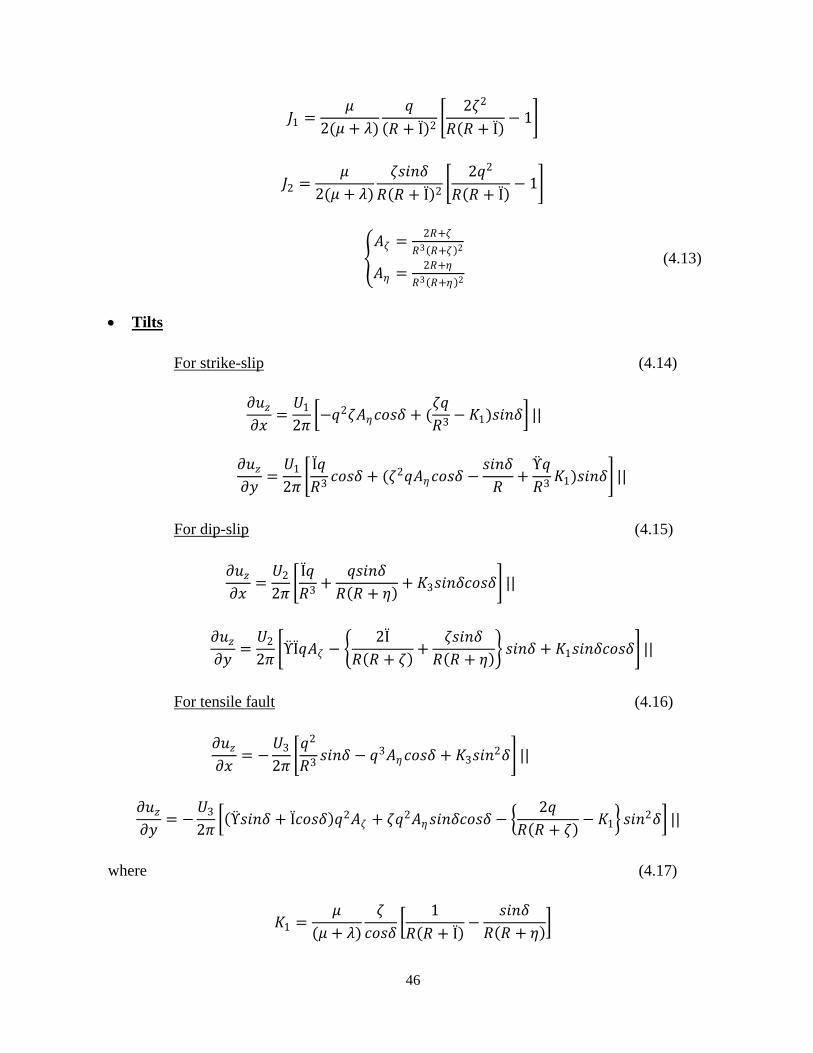
46

𝐽1 =𝜇

2(𝜇 + 𝜆)

𝑞

𝑅 + Ϊ 2

2휁2

𝑅 𝑅 + Ϊ − 1

𝐽2 =𝜇

2(𝜇 + 𝜆)

휁𝑠𝑖𝑛𝛿

𝑅 𝑅 + Ϊ 2

2𝑞2

𝑅 𝑅 + Ϊ − 1

𝐴휁 =

2𝑅+휁

𝑅3 𝑅+휁 2

𝐴휂 =2𝑅+휂

𝑅3 𝑅+휂 2

(4.13)

Tilts


𝜕𝑢𝑧

𝜕𝑥=

𝑈1

2𝜋 −𝑞2휁𝐴휂𝑐𝑜𝑠𝛿 + (

휁𝑞

𝑅3− 𝐾1)𝑠𝑖𝑛𝛿 ||

𝜕𝑢𝑧

𝜕𝑦=

𝑈1

2𝜋 Ϊ𝑞

𝑅3𝑐𝑜𝑠𝛿 + (휁2𝑞𝐴휂𝑐𝑜𝑠𝛿 −

𝑠𝑖𝑛𝛿

𝑅+

Ϋ𝑞

𝑅3𝐾1)𝑠𝑖𝑛𝛿 ||

For dip-slip (4.15)

𝜕𝑢𝑧

𝜕𝑥=

𝑈2

2𝜋 Ϊ𝑞

𝑅3+

𝑞𝑠𝑖𝑛𝛿

𝑅 𝑅 + 휂 + 𝐾3𝑠𝑖𝑛𝛿𝑐𝑜𝑠𝛿 ||

𝜕𝑢𝑧

𝜕𝑦=

𝑈2

2𝜋 ΫΪ𝑞𝐴휁 −

2Ϊ

𝑅 𝑅 + 휁 +

휁𝑠𝑖𝑛𝛿

𝑅 𝑅 + 휂 𝑠𝑖𝑛𝛿 + 𝐾1𝑠𝑖𝑛𝛿𝑐𝑜𝑠𝛿 ||


𝜕𝑢𝑧

𝜕𝑥= −

𝑈3

2𝜋 𝑞2

𝑅3𝑠𝑖𝑛𝛿 − 𝑞3𝐴휂𝑐𝑜𝑠𝛿 + 𝐾3𝑠𝑖𝑛

2𝛿 ||

𝜕𝑢𝑧

𝜕𝑦= −

𝑈3

2𝜋 Ϋ𝑠𝑖𝑛𝛿 + Ϊ𝑐𝑜𝑠𝛿 𝑞2𝐴휁 + 휁𝑞2𝐴휂𝑠𝑖𝑛𝛿𝑐𝑜𝑠𝛿 −

2𝑞

𝑅 𝑅 + 휁 − 𝐾1 𝑠𝑖𝑛2𝛿 ||

where (4.17)

𝐾1 =𝜇

(𝜇 + 𝜆)

휁

𝑐𝑜𝑠𝛿

1

𝑅 𝑅 + Ϊ −

𝑠𝑖𝑛𝛿

𝑅 𝑅 + 휂

47

𝐾2 =𝜇

(𝜇 + 𝜆) −

𝑠𝑖𝑛𝛿

𝑅+


𝑅 𝑅 + 휂 − 𝐾3

𝐾3 =𝜇

(𝜇 + 𝜆)

1

𝑐𝑜𝑠𝛿

𝑞

𝑅 𝑅 + 휂 −

Ϋ

𝑅 𝑅 + Ϊ

If 𝑐𝑜𝑠𝛿 = 0 (4.18)

𝐾1 =𝜇

(𝜇 + 𝜆)

휁𝑞

𝑅 𝑅 + Ϊ 2

𝐾3 =𝜇

(𝜇 + 𝜆)

𝑠𝑖𝑛𝛿

𝑅 + Ϊ[

휁2

𝑅 𝑅 + Ϊ − 1]

To avoid singularity in the above integrals,

if q=0, set 𝑡𝑎𝑛−1 휁휂

𝑞𝑅 to 0;

when 휁 = 0 set 𝐼5 to 0;

when R+η=0, which occurs when 𝑠𝑖𝑛𝛿 < 0 and 휁 = 𝑞 = 0 ,

set all terms containing R+η to 0

and replace ln(R+η) to -ln(R-η)

From the above integrals, surface displacements, strains, and tilts can be calculated as the result

of subsurface deformations being expressed as a combination of strike-slip, dip-slip, and

tensile fault deformations.

4.2 Inverse case

The main purpose of this research is to focus on solving the inverse case, which uses the

observation data obtained from the surface monitoring methods mentioned in section 3.5 and

reconstructs the distribution of the changes in volume that occur within the subsurface that

have resulted in the induced surface deformations. Measuring and recording surface

deformation data have become very fast and easy, with many methods available for monitoring

deformations. On the other hand, keeping track of the volume changes and the deformations

that occur within the reservoir rock, along with the changes in pressure, is very important

48

because these data help with the modeling and understanding of what is actually happening

within the reservoir and how it is responding to production. This data will also help in reservoir

management and in arranging the timing and quantity of production or water reinjection for

optimum results, in modeling deformation and fracture movements in waste injection projects,

and in studying subsurface displacements as a result of steam injection. Using surface data

observation points for back-calculating and determining reservoir compaction has therefore

become of great interest.

The approach for this thesis was to divide the reservoir into small rectangular elements. Based

on Geertsma (1973), volumetric changes inside the reservoir can be modeled as volume change

distribution in each element that occur in one direction. The surrounding medium, which is the

overburden material, is assumed to be a porous, elastic half-space, and the surface is assumed

to be stress free. Any observation point chosen on the surface thus has a deformation due to the

effect of volume changes occurring in each reservoir element. Of course this approach is

correct if the only source of deformation is the volume change in the reservoir. If not, the

deformations taking place at each observation point are the result of the effect of all sources of

deformation at different depths. In this study, as previously mentioned, it was assumed that the

changes in volume in the reservoir are the only source of deformation. Thus displacements and

tilts occurring at an observation point can be written as the summation of the effects of the

volume changes, either through expansion or compaction, that occur in each reservoir element.

Integrating these points in this way over the reservoir volume permits the calculation of the

deformations on the surface. From the equations mentioned in section 4.1 for calculating the

induced subsidence, it can be seen that the surface deformation can be described generally as

the following (Bilak, 1989):

𝑈𝑥(𝑟′) = 𝑈 𝑟, 𝑟′ .𝑣

𝐸𝑣 𝑟 . 𝑑𝑉𝑟 (4.19)

The mathematical approach used in this thesis is based on equation (4.19). 𝑈𝑥(𝑟′ ) is the

surface deformation or the induced subsidence at point 𝑟′ from the origin in a polar coordinate

system. 𝑈 𝑟, 𝑟′ represents Green’s function of the deformation (vertical deformation or tilts or

horizontal deformations, depending on the formula used) at a point 𝑟′ as a result of the

volumetric strain (𝐸𝑣)of a point source of 𝑟′ in the polar system in 𝑑𝑉𝑟 (Figure 13).

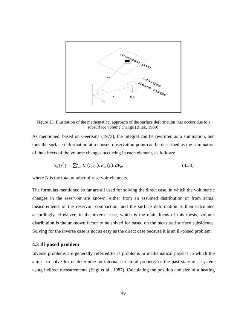
49

Figure 13: Illustration of the mathematical approach of the surface deformation that occurs due to a

subsurface volume change (Bilak, 1989).

As mentioned, based on Geertsma (1973), the integral can be rewritten as a summation, and

thus the surface deformation at a chosen observation point can be described as the summation

of the effects of the volume changes occurring in each element, as follows:

𝑈𝑥(𝑟′) = 𝑈𝑖 𝑟, 𝑟′ . 𝐸𝑣𝑖 𝑟 . 𝑑𝑉𝑟𝑖𝑁𝑖=1 (4.20)

where N is the total number of reservoir elements.

The formulas mentioned so far are all used for solving the direct case, in which the volumetric

changes in the reservoir are known, either from an assumed distribution or from actual

measurements of the reservoir compaction, and the surface deformation is then calculated

accordingly. However, in the inverse case, which is the main focus of this thesis, volume

distribution is the unknown factor to be solved for based on the measured surface subsidence.

Solving for the inverse case is not as easy as the direct case because it is an ill-posed problem.

4.3 Ill-posed problem

Inverse problems are generally referred to as problems in mathematical physics in which the

aim is to solve for or determine an internal structural property or the past state of a system

using indirect measurements (Engl et al., 1987). Calculating the position and size of a heating

50

source based on knowledge of the properties of the medium and the spatial distribution of the

surface temperature (Vasco, 2004) is an example of an ill-posed problem.

Many inverse problems can be described as a general form of

𝐴 ∗Z= 𝑢 (4.21)

where

u = the “external parameter” which is measured and known.

Z = the “internal parameter” which cannot be measured or is very hard to measure

directly.

A = in this case a given operator between u and Z.

In this thesis, u is the measured surface deformation, and Z, the internal parameter, is the

volume change occurring in the reservoir. A is the matrix relating volume changes to surface

deformations.

Equation (4.20), which is the general form for calculating surface subsidence from volume

changes is a form of Fredholm integral equation of the first kind with a kernel K(x,s)

(Tikhonov et al., 1977):

𝑢 𝑥 = 𝐾 𝑥, 𝑠 𝑍 𝑠 𝑑𝑠 𝑐 ≤ 𝑥 ≤ 𝑑𝑏

𝑎 (4.22)

Z(s) is the internal parameter or the unknown function in a space F. u(x) is the external

parameter or known function in a space U. The kernel K(x,s) is assumed to be continuous with

respect to variable x and also has a continuous partial derivative with respect to x (𝜕𝐾/𝜕𝑥).

Tikhonov and Arsenin (1977) rewrote the above integral using an operator of A:

𝐴 ∗ 𝑍 = 𝐾 𝑥, 𝑠 𝑍 𝑠 𝑑𝑠 𝑏

𝑎 (4.23)

The aim now is to solve for Z(s), the internal parameter. Assume that in an actual case of u(x)=

𝑢1 𝑥 there is a solution of 𝑍1 𝑠 in equation (4.22). This assumption means that, in this case,

a volume change of 𝑍1 𝑠 in the reservoir element has resulted in a surface deformation of

𝑢1 𝑥 :

51

𝑢1 𝑥 = 𝐾 𝑥, 𝑠 𝑍1 𝑠 𝑑𝑠 𝑏

𝑎(4.23.1)

However, in real and actual cases, the external parameter or the known factor, which is

measured and recorded experimentally by tools and engineering devices, would always contain

an error, no matter how exact and accurate the device is. This inaccuracy might be due to error

in the equipment itself, or in the set up, or in the reading of the data. Thus, rather than an exact

value or function for 𝑢1 𝑥 , only an approximation of the actual data u(x), that is slightly

different from 𝑢1 𝑥 , would be possible.

So now the approximate solution of the equation can be solved for, and the answer will be

close to 𝑍1 𝑠 and not exactly 𝑍 𝑥 . However, Tikhonov et al. (1977) showed that since

approximate data are used for 𝑢1 𝑥 , and 𝑢1 𝑥 ≠ 𝑢(𝑥), the exact function of 𝑍1 𝑠 cannot be

used for the approximate solution of equation (4.22), since the solution might not exist because

the kernel K(x, s) has a continuous derivative with respect to x, so 𝑢(𝑥) must also have a

continuous derivative with respect to x as well. If 𝑢(𝑥)does not have a continuous derivative

with respect to x, the solution to equation (4.22) will no longer exist. Furthermore, equation

(4.22) has a solution only if the approximate members of u(x) that belong to the image AF of

the set F of the function Z(s) under the mapping executed by the operator A, as mentioned, is as

follows:

𝑢 = 𝐴 ∗ 𝑍 ≡ 𝐾 𝑥, 𝑠 𝑍 𝑠 𝑑𝑠 , 𝑧(𝑠) ∈ 𝐹 𝑏

𝑎(4.24)

According to Tikhonov et al. (1977), the solution to equation (4.22) can be described in a

classic form based on equation (4.21) . The solution to the equation would thus be written as

𝑍 = 𝐴−1 ∗ 𝑢 (4.25)

In the equation (4.25), 𝐴−1 is not stable under small changes in the initial data (u in this case).

The problem is therefore referred to as ill-posed, and its solution is not straightforward, as is

usually the case for inverse cases. The known data is almost never the exact value and always

contains small error. This very small noise or slight discrepancies from the absolute exact

values in the initial observed data, which is the known data in the equation, would result in

large random variations in the solution for Z(s). In other words, small variations in the

52

observed data would result in large changes in the solution, thus making the solution unstable

even under very small changes in the input. The following example is a good illustration of the

effect of error in the known observation data on the solution (Bilak, 1989):

0.9999𝑥 + 1.0001𝑦 = 1

𝑥 − 𝑦 = 1

Thus 𝑥 = 0.5 and 𝑦 = −0.5

If an error of 𝛿 ≪ 1 is now added to the known part the result would be as follows:

0.9999𝑥 + 1.0001𝑦 = 1

𝑥 − 𝑦 = 1 + 𝛿

Thus 𝑥 = 0.5 + 5000𝛿 𝑦 = −0.5 + 4999.5𝛿

If equation 4.21 is non-singular, meaning that the determinant of A is not zero (det A≠ 0),

based on Cramer’s rule, it would have a unique solution. This result will be explained in more

detail in the following section. However, if the determinant of A is equal to zero (det A= 0)

and the equation is thus singular, a solution would be found (but would not be unique), only if

the condition for the existence of a solution is satisfied: vanishing of the relevant determinants.

The existence of the solution is then dependent only on the initial data set or the external factor

(Tikhonov et al., 1977).

As mentioned above, since exact values are not available, rather than dealing with equation

4.21, the following approximation equation would be used:

Ã ∗ 𝑍 = û (4.26)

where

𝗅𝗅Ã − 𝐴𝗅𝗅 < 𝛿 and 𝗅𝗅û − 𝑢𝗅𝗅 < 𝛿

Therefore the approximate matrix Ã must be considered rather than A, and it is thus more

difficult to determine whether the system is singular (Tikhonov et al., 1977). Since only the

approximate system Ã ∗ 𝑍 = û can be used, rather than the exact system(𝐴 ∗ 𝑍 = 𝑢), only an

53

approximate solution can be found. It should be remembered that this system must be stable

under small changes in the initial data in order for the equation to have a solution

For defining and providing a clear understanding of the concept and conditions of ill-posed

problems, describeing the conditions of a well-posed problem is helpful. In determining the

solution Z in space F from an initial observed data set of u in space U, the problem is well

posed on the pair of metric spaces (F,U) if the following conditions are satisfied (Tikhonov et

al., 1977):

For every element 𝑢 ∈ 𝑈 there exists a solution Z in the space F.

The solution is unique.

The problem is stable on the spaces (F,U).

Problems that do not satisfy these three conditions are known as ill-posed problems. It should

be pointed out that the term ill-posed is used with respect to a given pair of metric spaces

(Tikhonov et al., 1977), meaning that the same problem can be well posed in other matrixes

while being ill posed in (F, U).

With respect to the above conditions for a well-posed problem, the first two conditions

characterize the mathematical determinacy of a problem. The third condition, however, is

related to the physical determinacy of the problem and also implies the possibility of applying

numerical methods to solve it on the basis of approximate observation data (Tikhonov et al.,

1977).

The problem of solving a Fredholm integral equation of the first kind was proven by Tikhonov

et al. (1977) to be an ill-posed problem, and it was pointed out that the solution is unstable

under small changes in the observation data or in the known external parameter of u(x).

4.4 Ill-posed problems: the inverse case

Inverse cases make up a broad class of ill-posed problems in fields such as engineering,

physics, and technology. Observation data is gathered and processed as the external parameter

in the equation (4.21).The data processing is generally carried out in three steps (Tikhonov et

al., 1977):

54

Data are gathered or read from a measurement device.

The results are processed statistically with an estimate of the degree of reliability.

The results from step two are interpreted.

The goal is now to use the final data as u(x) to solve equation (4.21).

Suppose that the phenomenon has occurred and can be characterized by an element of 𝑍𝑇

belonging to a set F. The result would be 𝐴 ∗ 𝑍𝑇 = 𝑢𝑇 . Here 𝑢𝑇 ∈ 𝐴𝐹, and AF is the image of

the set F under the mapping executed by the operator A. 𝑍𝑇 can not be measured or it is hard to

measure, and thus only the resulting effect of it, 𝑢𝑇, is measured and known. It can thus be

described as an inverse case. Equation (4.21) has a solution on F only for observed data points

that belong to the set of AF. The value of 𝑢𝑇 is obtained from observation and measured data,

and thus only the approximate value is known. Thus only an approximate solution can be used

to solve for a value close to 𝑍𝑇 (Tikhonov et al., 1977).

𝐴 ∗ 𝑍 = û (4.27)

û, the approximate external parameter, does not usually belong to the set of AF. Moreover, the

operator A is usually defined in such a way that it’s inverse, 𝐴−1, is not continuous. Thus, it

might not have a solution for two reasons (Tikhonov et al., 1977):

The approximate solution might not exist on the set of F since û might not belong to the

set of AF, and the first requirement of well-posed problems is not satisfied.

Even if the solution does exist, the stability requirement is not satisfied. That is, the

solution would not be stable under small changes in the external parameter because the

inverse matrix 𝐴−1 is not continuous. The third requirement of well-posed problems is

therefore not met.

Thus, inverse problems in which the input is measured data, and therefore only an

approximation of the actual value is available, are ill-posed problems. Therefore, the inverse

case that is the focus of this thesis, which is the calculation of the changes in volume based on

surface observation data, is an ill-posed problem. To solve and model the volume changes, the

reservoir is divided into small elements. Each element represents the volume changes that

cause deformations. This assumption is correct since the depth of the reservoir is much larger

55

than the dimensions of each element (Bilak, 1989). Thus, the deformation at each observation

point is the summation of the effects of the volume changes occurring in each element:

𝑢𝑚 = 𝐾𝑚 ,𝑛 ∗ ∆𝑣𝑛𝑁𝑛=1 (4.28)

𝑢𝑚= surface observation data from the 𝑚𝑡𝑕 observation point, which in this thesis can be the

vertical displacement or tilt1 or tilt2

N = number of reservoir elements

∆𝑣𝑛= volume change in the 𝑛𝑡𝑕 reservoir element

Equation (4.28) can be written in the form of a matrix, as follows:

𝐾 𝑚∗𝑛 ∗ ∆𝑣 𝑛∗1 = 𝑢 𝑚∗1 (4.29)

To solve for the unknown matrix ∆𝑣 𝑛∗1,

∆𝑣 𝑛∗1 = 𝑢 𝑚∗1 ∗ 𝐾 𝑚∗𝑛−1

(4.30)

A straightforward solution for a well-posed inverse linear problem would be to use Cramer’s

rule to solve for ∆𝑣. The following is a general example for a reservoir with two elements and

three observation points on the surface:

A reservoir of two elements is assumed with three observation points on the surface. The

unknowns are the volume changes in each element, so two unknowns are present. The format

of the equation to be solved is as follows:

𝐾11 𝐾12

𝐾21 𝐾22

𝐾31 𝐾32

∗ ∆𝑣1

∆𝑣2 =

𝑈1

𝑈2

𝑈3

where ∆𝑣1 and ∆𝑣2 are the unknowns.

Using Cramer’s rule would result in

∆𝑣1 =det 𝐾1

det 𝐾

56

∆𝑣2 =det 𝐾2

det 𝐾

where

𝐾 = 𝐾11 𝐾12

𝐾21 𝐾22

𝐾31 𝐾32

and

𝐾1 = 𝑈1 𝐾12

𝑈2 𝐾22

𝑈3 𝐾32

and 𝐾2 = 𝐾11 𝑈1

𝐾21 𝑈2

𝐾31 𝑈3

The general form for 𝐾1 and 𝐾2 is as follows:

𝐾1 =

𝑈1 𝐾12 𝐾13

𝑈2 𝐾22 𝐾23

𝑈3 𝐾32 𝐾33

………

𝐾2 =

𝐾11 𝑈1 𝐾13

𝐾21 𝑈2 𝐾23

𝐾31 𝑈3 𝐾33

………

𝐾3 = 𝐾11 𝐾12 𝑈1

𝐾21 𝐾22 𝑈2

𝐾31 𝐾32 𝑈3

………

∆𝑣1 =det 𝐾1

det 𝐾 ∆𝑣2 =

det 𝐾2

det 𝐾 ∆𝑣3 =

det 𝐾3

det 𝐾 …∆𝑣𝑛 =

det 𝐾𝑛

det 𝐾

As can be seen for the solution of the volume changes, if the determinant of the K matrix is

zero or close to zero, the result of Δv would go to infinity and thus there would be no solution,

meaning that the problem would be ill-posed.

det 𝑘 = 𝑘

If 𝑘 → 0

∆𝑣𝑛 =|𝐾𝑛 |

|𝐾|→ ∞

57

The elements of the K matrix can be described as

𝐾(𝑥1 , 𝑆1) 𝐾(𝑥1 , 𝑆2) …𝐾(𝑥2 , 𝑆1) 𝐾(𝑥2, 𝑆2) …

… … …

As the number of reservoir elements increases, the size of the elements decreases, and the

distance between each point would become too small. As a result, the two columns in the K

matrix would be very similar, and as the number of elements increases, the columns in the K

matrix would become close to identical. Thus, in a reservoir that has a large number of

elements, 𝑘 → 0 as the number of reservoir elements increases (Rothenburg, 2009, personal

communication). Therefore, the problem is ill-posed, and in order to solve for the volume

changes the system must be changed into a well-posed system that is not singular and is stable

under small changes in the input.

4.5 Regularization technique

As mentioned in previous sections, this thesis deals with an ill-posed problem. The major

factor that causes the problem to be characterized as ill-posed is the approximate nature of the

observation data points available and the known information, which thus results in u being

outside the set of AF. Tikhonov et al. (1977) called these types of problems genuinely ill-posed

problems. A method of dealing with such problems is to construct approximate solutions for

the following equation:

𝐴 ∗ 𝑍 = 𝑢 (4.21)

Tikhonov et al. (1977) introduced the concept of the regularization as an approach for finding

an approximate solution for these types of problems. The solution being constructed must be

stable under small changes in the initial observed data. As approximate data 𝑢𝛿 , and not the

exact value 𝑢𝑇 , observation points might be outside AF. Thus 𝐴−1 would not be continuous,

and the solution would not exist. If the approximate and the exact values differ from each other

by no greater than δ, 𝑢𝛿 − 𝑢𝑇 < 𝛿, 𝛿 being the difference between the exact value and the

observed value, the data used as input would basically be the error present in the observation

point. Since 𝑢𝛿 ≠ 𝑢𝑇 , the above exact equation cannot be used to solve for the approximate

volume change of 𝑍𝛿 . That is,

58

𝑍𝛿 = 𝐴−1 ∗ 𝑢𝛿 (4.31)

Calculation of 𝑍𝛿 requires the use of an operator that is dependent on or in accordance with the

error, which means that when the error is too small and 𝛿 → 0, the approximate solution must

approach the exact solution (𝑍𝛿 → 𝑍𝑇) (Tikhonov et al., 1977).

Suppose that elements of 𝑍𝑇 ∈ 𝐹 and 𝑢𝑇 ∈ 𝑈 and that 𝑍𝑇 and 𝑢𝑇 are connected by A matrix as

𝐴 ∗ 𝑍𝑇 = 𝑢𝑇, Thus:

An operator of R(𝑢, 𝛽) is defined by Tikhonov et al. (1977) as a regularizing operator for the

general form of the above equation (A*Z=u) in the neighbourhood of 𝑢 = 𝑢𝑇 if an approximate

solution for 𝑍𝛽 = 𝑅(𝑢𝛿 , 𝛽) can be found using the approximate known data of 𝑢𝛿 and with the

aid of the regularization operator (R(𝑢, 𝛽)). Here 𝛽=𝛽(δ, 𝑢𝛿 ), which is in accordance with the

error present in the observed data(δ). The solution is referred to as the regularized solution and

the numerical parameter 𝛽 is called the regularization parameter.

There may be many operators R(u,𝛽) from U into F that are dependent on parameter 𝛽 and are

defined for every element of U and every positive value of 𝛽. However, another characteristic

of the regularizing operator is that it should be continuous with respect to u as well. Tikhonov

et al. (1977) proved the following theorem:

Theorem: Let A denote an operator from F into U, and let R(u,𝛽) denote an operator from U

into F that is defined for every element u of U and every positive value of 𝛽 and

that is continuous with respect to u. If

lim𝛽→0

𝑅 𝐴𝑍, 𝛽 = 𝑍

for every element Z of F, then the operator R(u,𝛽) is a regularizing operator for the

equation

𝐴 ∗ 𝑍 = 𝑢.

To summarize, every regularizing operator of R characterizes approximate construction of

stable solution provided that the value of 𝛽 is in accordance with and consistent with the

accuracy δ of the observed data (𝛽=(δ)). Since 𝑢𝛿 − 𝑢𝑇 < 𝛿, the regularization parameter

59

can be chosen in such a way that as the error moves toward zero (δ→ 0), meaning that the

approximate value of the input data approaches the absolute actual value, the regularized

solution of 𝑍𝛽 = 𝑅(𝑢𝛿 , 𝛽 𝛿 ) would approach the exact solution of 𝑍𝑇 , and thus,

|𝑍𝑇 − 𝑍𝛽 | → 0

Thus, to find an approximate solution for the equation (4.21) that is stable under small changes

in the initial observed data points requires the following:

1. Define a regularizing operator R.

2. Verify the regularization parameter 𝛽 using supplementary information related to the

problem, for example, pertaining to the size of the error present in the input observed

data.

As mentioned in previous sections, the problem this thesis deals with, which is calculating

reservoir deformations and volume changes using surface deformation data, is a Fredholm

integral of the first type. Due to the ill-posed nature of the integral, a solution might not exist,

and thus, to solve the problem, an approximate solution should be used. Based on Tikhonov et

al. (1977), the solution of another problem that is stable and is close to the original problem can

be used for small values of error in the observed input data. Rather than the initial equation

having to be solved, another problem is thus chosen, and the solution to that equation would be

the approximate solution of the initial ill-posed problem. The problem now to be solved would

be

𝑢 𝑥 = {𝑈 ∗𝐸𝑣 ∗ 𝑑𝑣 + 𝛽 ∗ 𝑅(𝐸𝑣)} (4.32)

The next steps would then be to find the suitable regularization operator for the Fredholm

integral and to define the regularization parameter of 𝛽.

4.5.1 Defining 𝛽

𝛽 is a number between zero and one, which is obtained through trial and error. If the value of 𝛽

used is a very small value or zero, the second term added to the initial ill-posed equation to

make it stable would be omitted, and the equation would still be the same initial ill-posed

problem, with a large amount of noise observable in the results. However, using a very large

60

value of 𝛽 would significantly affect the solution and would result in a smooth solution that is

not correct (Figure 14).

Figure 14: The effect of the value of 𝛽 on the solution of the inverse problem (Dusseault et al., 2002).

4.5.2 Construction of the regularization operator

One possible approach to the construction of a regularization operator that is suitable for the

Fredholm integral is using the least square approach. If the functional referred to as the

smoothing functional is minimized, the regularization operator can be defined. The procedure

is described in detail as follows.

If δ=0 and thus no error is present in the observed data points, the following is correct:

𝑢 𝑥 = 𝑈 ∗𝐸𝑣 ∗ 𝑑𝑣

As mentioned, the above equation can be described as a general form of the Fredholm integral:

𝑢(𝑥) = 𝑘 𝑥, 𝑠 ∗ 𝑍 𝑠 ∗ 𝑑𝑠

However, the measured observation data are not the actual exact values. If the right-hand side

of the equation is the exact solution resulting in the precise value of Z, thus different from the

observation point:

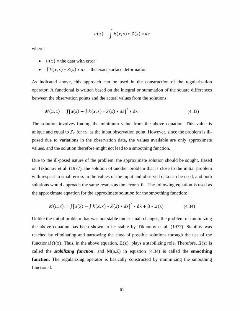
61

𝑢 𝑥 − 𝑘 𝑥, 𝑠 ∗ 𝑍 𝑠 ∗ 𝑑𝑠

where

𝑢 𝑥 = the data with error

𝑘 𝑥, 𝑠 ∗ 𝑍 𝑠 ∗ 𝑑𝑠 = the exact surface deformation

As indicated above, this approach can be used in the construction of the regularization

operator. A functional is written based on the integral or summation of the square differences

between the observation points and the actual values from the solutions:

𝑀 𝑢, 𝑧 = [u x − 𝑘 𝑥, 𝑠 ∗ 𝑍 𝑠 ∗ 𝑑𝑠]2∗ dx (4.33)

The solution involves finding the minimum value from the above equation. This value is

unique and equal to 𝑍𝑇 for 𝑢𝑇 as the input observation point. However, since the problem is ill-

posed due to variations in the observation data, the values available are only approximate

values, and the solution therefore might not lead to a smoothing function.

Due to the ill-posed nature of the problem, the approximate solution should be sought. Based

on Tikhonov et al. (1977), the solution of another problem that is close to the initial problem

with respect to small errors in the values of the input and observed data can be used, and both

solutions would approach the same results as the error→ 0. The following equation is used as

the approximate equation for the approximate solution for the smoothing function:

𝑀 𝑢, 𝑧 = [𝑢 x − 𝑘 𝑥, 𝑠 ∗ 𝑍 𝑠 ∗ 𝑑𝑠]2∗ dx + β ∗ Ω(z) (4.34)

Unlike the initial problem that was not stable under small changes, the problem of minimizing

the above equation has been shown to be stable by Tikhonov et al. (1977). Stability was

reached by eliminating and narrowing the class of possible solutions through the use of the

functional Ω(z). Thus, in the above equation, Ω(z) plays a stabilizing role. Therefore, Ω(z) is

called the stabilizing function, and M(u,Z) in equation (4.34) is called the smoothing

function. The regularizing operator is basically constructed by minimizing the smoothing

functional.

62

If F, which is a set of possible solutions of the equation A*Z=u, is assumed to be a matrix space

and Ω(z) is a stabilizing functional defined on a set 𝐹1 ⊂ 𝐹, then the following would apply

(Tikhonov et al., 1977):

Theorem: Let A denote a continuous operator from F into U for every element u of U and

every positive parameter 𝛽, there exists an element 𝑍𝛽 ∈ 𝐹1 for which the functional

𝑀 𝑢, 𝑧 = [𝑢 x − 𝑘 𝑥, 𝑠 ∗ 𝑍 𝑠 ∗ 𝑑𝑠]2

∗ dx + β ∗ Ω(z)

attains its greatest lower bound.

Tikhonov et al. (1977) introduced the following stabilizing functional:

𝛺 𝑧 = 𝑞𝑟 𝑥 ∗ (𝑑𝑟𝑧

𝑑𝑥 𝑟)2𝑑𝑥𝑝𝑟=0

𝑏

𝑎 (4.35)

They proved that it is the smoothest function up to the order of p for which |AZ-u|=δ. Thus, the

general form of the smoothing function using the above stabilizing function of the first order,

p=1, would be

𝑀 𝑢, 𝑧 = [𝑢 x − [𝑘 𝑥, 𝑠 ∗ 𝑍 𝑠 ∗ 𝑑𝑠]]𝑏

𝑎

d

c

2

∗ dx + β ∗ 𝑞𝑟 𝑥 ∗ (𝑑𝑟𝑧

𝑑𝑥𝑟)2𝑑𝑥

1

𝑟=0

𝑏

𝑎

𝑐 ≤ 𝑥 ≤ 𝑑

In the above equation, q(s) is a continuous function, is defined randomly, and can be used to

modify the solution functions of Z(s). The result would be the following:

𝑀 𝑢, 𝑧 = [𝑢 x − [𝑘 𝑥, 𝑠 ∗ 𝑍 𝑠 ∗ 𝑑𝑠]]𝑏

𝑎

d

c

2

∗ dx + β

∗ 𝑞0 𝑥 ∗ 𝑍2 𝑠 + 𝑞1 𝑥 ∗ (𝑑𝑧

𝑑𝑥)2 ∗ 𝑑𝑥

𝑏

𝑎

63

The graph in Figure 15 shows the results of the solution of an ill-posed problem along with the

actual expected values at 𝛽=0.

Figure 15: Results of the inverse calculations, showing a large number of jumps, especially at the corner

points; the solution is therefore not smooth (Rothenburg, 2009, personal communication).

The smooth curve represents the actual subsurface deformation, and the graph with noise

illustrates the result of the ill-posed solution when 𝛽=0. The goal is thus to smoothen the

solution. As can be seen, the corner points contain a greater degree of inaccuracy and therefore

more noise in the results than the middle points. A value of q must be chosen that will

smoothen the entire solution. On the other hand, outside the range of the actual values, there

will still be noise while the expected value is supposed to be zero. However, it is not desirable

to force the solution to be zero outside the range.

Therefore, q=1 and 𝑞0 = 0 were chosen for smoothening the solution (Rothenburg, 2009,

personal communication)

𝑀 𝑢, 𝑧 = [𝑢 x − [𝑘 𝑥, 𝑠 ∗ 𝑍 𝑠 ∗ 𝑑𝑠]]𝑏

𝑎

d

c

2

∗ d𝑥 + β ∗ 0 ∗ 𝑍2 𝑠 + 1 ∗ (𝑑𝑍


𝑏

𝑎

For the Fredholm integral of the first kind, Tikhonov defined the stabilizing function to be used

in the above equation as follows:

𝛺 𝑧 = 𝑞(𝑠) ∗ (𝑑𝑍(𝑠)

𝑑𝑠)2𝑑𝑠

This format is basically the general form of the function used in the previous equation.

64

As mentioned, the initial aim in solving for the ill-posed problem was to determine the

regularization operator, 𝑍𝛽 = 𝑅(𝑢𝛿 , 𝛽). The approach used is to minimize the smoothest

function. Thus, taking the first derivative of equation (4.34) with respect to x would result in

the following:

𝜕𝑀(𝑍, 𝑢)

𝜕𝑥= [𝑢 𝑥 − 𝐾 𝑥, 𝑠 ∗ 𝑍 𝑠 ∗ 𝑑𝑠]2 + 𝛽 (

𝑑𝑍

𝑑𝑠)2 ∗ 𝑑𝑠

For the minimum to exist, the derivative must be set to zero. Thus,

𝜕𝑀(𝑍, 𝑢)

𝜕𝑥= [𝑢 𝑥 − 𝐾 𝑥, 𝑠 ∗ 𝑍 𝑠 ∗ 𝑑𝑠]2 + 𝛽

𝑑𝑍

𝑑𝑠

2

∗ 𝑑𝑠 = 0

The first part of the equation, [𝑢 𝑥 − 𝐾 𝑥, 𝑠 ∗ 𝑍 𝑠 ∗ 𝑑𝑠]2, is always nonnegative. As for

the second part, 𝛽 𝑑𝑍

𝑑𝑠

2∗ 𝑑𝑠, 𝛽 being always positive and the integral a power of two, thus

always nonnegative. Therefore, for the entire derivative to be equal to zero and for a minimum

to exist, both sentences must be zero.

Since, as previously mentioned, the thickness of a reservoir is much smaller than its width and

length, it can be modeled as a thin plate. It is thus correct to assume that we are dealing with a

two dimensional. Thus, (𝑑𝑍

𝑑𝑠)2 can be written as (

𝑑2𝐸𝑣

𝑑𝑥 2 +𝑑2𝐸𝑣

𝑑𝑦 2 ), so in the problem of surface

deformation analysis, the derivative of the Fredholm integral would be defined as follows:

𝑢 𝑥 − 𝑢.𝑣

𝐸𝑣 . 𝑑𝑣 + 𝛽 𝑑2𝐸𝑣

𝑑𝑥 2 +𝑑2𝐸𝑣

𝑑𝑦 2 = 0 (4.36)

As can be seen, the parameter is a function of the two variables x and y. The regularization

operator that would result in the best approximate solution to the ill-posed problem of solving

for the reservoir’s volume changes using surface deformation data would be the Laplacian

operator:

(𝑑2𝐸𝑣

𝑑𝑥2+

𝑑2𝐸𝑣

𝑑𝑦2)

65

in which 𝐸𝑣𝛽 is the set of back-calculated volume changes with respect to the initial error in

the input observation data. For 𝐸𝑣𝛽 = 𝑅(𝑢𝛿 , 𝛽) to satisfy the existence of the solution for the

minimum of equation (4.34) to be obtainable, the following must apply:

𝑑2𝐸𝑣

𝑑𝑥2+

𝑑2𝐸𝑣

𝑑𝑦2 = 0

Tikhonov et al. (1977) showed that for the Laplacian operator, the equation (4.36) has a unique

solution for 𝐸𝑣𝛽 that is continuous for all values of 𝛽. If 𝛽=0,

𝑀 𝑢, 𝑧 = [𝑢 x − [𝑘 𝑥, 𝑠 ∗ 𝑍 𝑠 ∗ 𝑑𝑠]]𝑏

𝑎

d

c

2

∗ d𝑥 + 0 ∗ 0 ∗ 𝑍2 𝑠 + 1 ∗ (𝑑𝑍


𝑏

𝑎

and

𝑀 𝑢, 𝑧 = [𝑢 x − [𝑘 𝑥, 𝑠 ∗ 𝑍 𝑠 ∗ 𝑑𝑠]]𝑏

𝑎

d

c

2

∗ d𝑥

This equation would be the initial ill-posed problem. The solution would thus be the solution of

the original equation which might not exist. For small values of 𝛽, the solution would be an

approximate solution of the original equation.

The initial matrix form of the problem, which was

𝐾 𝑚∗𝑛 ∗ ∆𝑣 𝑛∗1 = 𝑈 𝑚∗1

is rewritten, and if the Lapacian operator and the regularization coefficient are added to the

original equation, the following would be obtained

𝐾 𝑀∗𝑁 ∗ ∆𝑣 𝑁∗1 − 𝛽 ∗ [𝐿𝑎𝑝𝑙𝑎𝑐𝑒]𝑁∗𝑁 ∗ ∆𝑣 𝑁∗1 = 𝑈 𝑚∗1 (4.37)

Thus,

( 𝐾 𝑀∗𝑁 − 𝛽 ∗ [𝐿𝑎𝑝𝑙𝑎𝑐𝑒]𝑁∗𝑁) ∗ ∆𝑣 𝑁∗1 = 𝑈 𝑚∗1 (4.37.1)

66

As mentioned previously, the reservoir can be assumed to be divided into small elements and

the changes in volume in the reservoir thus be described as the summation of the changes in

volume that occur in each element. The initial smoothing function, which was an integrated

formula, can therefore be written as a series of summations.

Ø = (𝑈𝑚 − 𝐾𝑚𝑛 ∗ ∆𝑣𝑛)𝑁𝑛=1

2𝑀𝑚=1 (4.38)

This equation therefore represents the initial problem, where

M = total number of observation points on the surface

N = total number of reservoir elements

𝐾𝑚𝑛 = matrix relating volume changes in the 𝑛𝑡𝑕 reservoir element to surface

deformations occurring in the 𝑚𝑡𝑕 point on the surface grid

∆𝑣𝑛 = volume change in the 𝑛𝑡𝑕 reservoir element

𝑈𝑚= observation data (deformation, i.e., vertical displacement, tilts) in the

𝑚𝑡𝑕observation point

However, due to the noise in the observation data, 𝑈𝑚 , the problem of minimizing the equation

and solving it would not have a solution since it is not stable under small changes. Thus, the

stabilizing function, which in the case of a Fredholm integral of the first type is a Laplacian

operator, should be added to the equation as proven above. The summation form of the

problem to be solved would thus be


2+ 𝛽 ∗ (0 − 𝐿𝑛𝑗 ∗ ∆𝑣𝑗 )𝑁

𝑗=12𝑁

𝑛=1𝑀𝑚=1 (4.39)

The goal is to find solutions that will minimize Ø.

4.6 Calculating the general matrix equation form of the problem

The inverse problem of solving for the reservoir volumetric changes using surface data was

reduced to minimizing the following equation:


2+ 𝛽 ∗ (0 − 𝐿𝑛𝑗 ∗ ∆𝑣𝑗 )𝑁

𝑗=12𝑁

𝑛=1𝑀𝑚=1 (4.39)

This equation can be written in two main parts:

67

Ø = 𝐼 + 𝐼𝐼

where

𝐼 = (𝑈𝑚 − 𝐾𝑚𝑛 ∗ ∆𝑣𝑛)

𝑁

𝑛=1

2𝑀

𝑚=1

𝐼𝐼 = 𝛽 ∗ (0 − 𝐿𝑛𝑗 ∗ ∆𝑣𝑗 )

𝑁

𝑗=1

2𝑁

𝑛=1

To minimize the equation,

𝜕Ø

𝜕𝑣𝑖=

𝜕𝐼

𝜕𝑣𝑖+

𝜕𝐼𝐼

𝜕𝑣𝑖

where 𝜕𝑣𝑖 is the volume change in the 𝑖𝑡𝑕 reservoir element. Thus, for the general case of a

reservoir with N number of elements and M, being the total number of observation points the

following would result:

Part 𝐈:

𝐼 = (𝑈𝑚 − 𝑘𝑚𝑛 ∗ ∆𝑣𝑛)

𝑁

𝑛=1

2𝑀

𝑚=1

𝐼 = (𝑈1 − 𝑘11 ∗ ∆𝑣1 + 𝑘12 ∗ ∆𝑣2 + 𝑘13 ∗ ∆𝑣3 + ⋯ + 𝑘1𝑁 ∗ ∆𝑣𝑁 )2 + (𝑈2 − 𝑘21 ∗ ∆𝑣1 + 𝑘22 ∗

∆𝑣2+𝑘23∗∆𝑣3+…+𝑘2𝑁∗∆𝑣𝑁)2+…+(𝑈𝑀−𝑘𝑀1∗∆𝑣1+𝑘𝑀2∗∆𝑣2+𝑘𝑀3∗∆𝑣3+…+𝑘𝑀𝑁∗∆𝑣𝑁)2

𝜕𝐼

𝜕𝑣1= 2 ∗ 𝑈1 − (𝑘11 ∗ ∆𝑣1 + 𝑘12 ∗ ∆𝑣2 + 𝑘13 ∗ ∆𝑣3 + ⋯ + 𝑘1𝑁 ∗ ∆𝑣𝑁 ] ∗ 𝑘11 + 2 ∗

𝑈2 − 𝑘21 ∗ ∆𝑣1 + 𝑘22 ∗ ∆𝑣2 + 𝑘23 ∗ ∆𝑣3 + ⋯ + 𝑘2𝑁 ∗ ∆𝑣𝑁 ∗ 𝑘21 + ⋯ + 2 ∗ [𝑈𝑀 −

𝑘𝑀1 ∗ ∆𝑣1 + 𝑘𝑀2 ∗ ∆𝑣2 + 𝑘𝑀3 ∗ ∆𝑣3 + ⋯ + 𝑘𝑀𝑁 ∗ ∆𝑣𝑁 ∗ 𝑘𝑀1] = 0

𝜕𝐼

𝜕𝑣2= 2 ∗ 𝑈1 − (𝐾11 ∗ ∆𝑣1 + 𝐾12 ∗ ∆𝑣2 + 𝐾13 ∗ ∆𝑣3 + ⋯ + 𝐾1𝑁 ∗ ∆𝑣𝑁 ] ∗ 𝐾12 + 2 ∗

𝑈2 − 𝐾21 ∗ ∆𝑣1 + 𝐾22 ∗ ∆𝑣2 + 𝐾23 ∗ ∆𝑣3 + ⋯ + 𝐾2𝑁 ∗ ∆𝑣𝑁 ∗ 𝐾22 + ⋯ + 2 ∗ [𝑈𝑀 −

𝐾𝑀1 ∗ ∆𝑣1 + 𝐾𝑀2 ∗ ∆𝑣2 + 𝐾𝑀3 ∗ ∆𝑣3 + ⋯ + 𝐾𝑀𝑁 ∗ ∆𝑣𝑁 ∗ 𝐾𝑀2] = 0

...

68

The general matrix form of the above equations would be

𝐾 𝑁∗𝑁 ∗ ∆𝑣 𝑜𝑟 𝑡𝑕𝑒 𝑢𝑛𝑘𝑛𝑜𝑤𝑛 𝑁∗1 = 𝑈 𝑜𝑟 𝑇𝑕𝑒 𝐴𝑛𝑠𝑤𝑒𝑟 𝑚𝑎𝑡𝑟𝑖𝑥 𝑁∗1

where

𝐾 =

𝑘𝑖1 2𝑀

𝑖=1 𝑘𝑖1 ∗ 𝑘𝑖2𝑀𝑖=1 𝑘𝑖1 ∗ 𝑘𝑖3 … 𝑀

𝑖=1

𝑘𝑖1 ∗ 𝑘𝑖2𝑀𝑖=1 𝑘𝑖2

2𝑀𝑖=1 𝑘𝑖2 ∗ 𝑘𝑖3

𝑀𝑖=1 …

𝑘𝑖1 ∗ 𝑘𝑖3𝑀𝑖=1 𝑘𝑖2 ∗ 𝑘𝑖3

𝑀𝑖=1 𝑘𝑖3

2𝑀𝑖=1 …

⋮

𝑁∗𝑁

As can be seen, K matrix is a symmetric matrix.

∆𝑣𝑖 = ∆𝑣1

…∆𝑣𝑁

U= 𝑘𝑖1 ∗ 𝑢𝑖

𝑀𝑖=1

⋮ 𝑘1𝑁 ∗ 𝑢𝑖

𝑀𝑖=1

where 𝑢𝑖 is the observation data from the 𝑖𝑡𝑕 observation point.

For the second part,

𝐼𝐼 = 𝛽 ∗ (0 − 𝐿𝑛𝑗 ∗ ∆𝑣𝑗 )

𝑁

𝑗=1

2𝑁

𝑛=1

Part II:

𝜕𝐼𝐼

𝜕𝑣1= 2𝛽 ∗ 0 − (𝐿11 ∗ ∆𝑣1 + 𝐿12 ∗ ∆𝑣2 + 𝐿13 ∗ ∆𝑣3 + ⋯ + 𝐿1𝑁 ∗ ∆𝑣𝑁 ] ∗ 𝐿11 + 2𝛽

∗ 0 − 𝐿21 ∗ ∆𝑣1 + 𝐿22 ∗ ∆𝑣2 + 𝐿23 ∗ ∆𝑣3 + ⋯ + 𝐿2𝑁 ∗ ∆𝑣𝑁 ∗ 𝐿21 + ⋯ + 2𝛽

∗ [0 − 𝐿𝑁1 ∗ ∆𝑣1 + 𝐿𝑁2 ∗ ∆𝑣2 + 𝐿𝑁3 ∗ ∆𝑣3 + ⋯ + 𝐿𝑁𝑁 ∗ ∆𝑣𝑁 ∗ 𝐿𝑁1] = 0

𝜕𝐼𝐼

𝜕𝑣2= ⋯

The general matrix of L from the above equations would thus be as follows:

69

𝐿 = 𝛽 ∗

𝐿𝑖1

2

𝑁

𝑖=1

𝐿𝑖1 ∗ 𝐿𝑖2

𝑁

𝑖=1

𝐿𝑖1 ∗ 𝐿𝑖3 …

𝑁

𝑖=1


𝑁

𝑖=1

𝐿𝑖2 2

𝑁

𝑖=1


𝑁

𝑖=1

…


𝑁

𝑖=1


𝑁

𝑖=1

𝐿𝑖3 2

𝑁

𝑖=1

…

⋮

The general form of the second part in matrix form would then be

−𝛽 ∗ 𝐿 𝑁∗𝑁 ∗ ∆𝑣 𝑜𝑟 𝑡𝑕𝑒 𝑢𝑛𝑘𝑛𝑜𝑤𝑛 𝑁∗1 = 0

To summarize, the initial problem, which was𝜕Ø

𝜕𝑣 𝑖= 0, would be written in the form of the

following matrix problem:

𝐾 𝑁∗𝑁 ∗ ∆𝑣 𝑜𝑟 𝑡𝑕𝑒 𝑢𝑛𝑘𝑛𝑜𝑤𝑛 𝑁∗1 − 𝛽 ∗ 𝐿 𝑁∗𝑁 ∗ ∆𝑣 𝑜𝑟 𝑡𝑕𝑒 𝑢𝑛𝑘𝑛𝑜𝑤𝑛 𝑁∗1

= 𝑈 𝑜𝑟 𝑇𝑕𝑒 𝐴𝑛𝑠𝑤𝑒𝑟 𝑚𝑎𝑡𝑟𝑖𝑥 𝑁∗1

𝐾 − 𝛽𝐿 𝑁∗𝑁 ∗ ∆𝑣 𝑜𝑟 𝑡𝑕𝑒 𝑢𝑛𝑘𝑛𝑜𝑤𝑛 𝑁∗1 = 𝑈 𝑜𝑟 𝑇𝑕𝑒 𝐴𝑛𝑠𝑤𝑒𝑟 𝑚𝑎𝑡𝑟𝑖𝑥 𝑁∗1 (4.40)

This would be the matrix to solve.

4.7 Solving the matrix equation

4.7.1 Singular value decomposition method

To solve the matrix equation, the singular value decomposition (SVD) method was used. This

method is used for solving or dealing with sets of equations or matrix systems that are either

singular or numerically very close to being singular. Unlike some other techniques used for

dealing with a set of equations, SVD not only diagnoses the problem but also solves it.

The SVD method is based on the theorem of linear algebra. Any A matrix of M*N that M≥N

can be written as the product of three metrics as follows:

70

𝐴 𝑀∗𝑁 = 𝑈 𝑀∗𝑁 ∗

𝑤1

0000

0𝑤2

000

00𝑤3

00

000⋱0

0000

𝑤𝑁

𝑁∗𝑁

∗ 𝑉𝑇 𝑁∗𝑁

Alternatively, each element of A matrix can be written as

𝐴𝑖𝑗 = 𝑤𝑘 ∗ 𝑈𝑖𝑘 ∗ 𝑉𝑗𝑘

𝑁

𝐾=1

where

[𝑈]𝑀∗𝑁 is a column-orthogonal matrix.

[𝑊]𝑁∗𝑁 is a diagonal matrix with positive or zero elements. These elements are the

singular values.

[𝑉𝑇]𝑁∗𝑁 is the transpose of an N*N orthogonal matrix of V.

The SVD method can also be applied for cases when M<N but the decomposition matrixes are

slightly different from what mentioned above. Details can be found in Press et al. (1988) .

As mentioned, the general form of an inverse problem would be

𝐴 ∗ 𝑍 = 𝑈

The issues with ill-posed problems are as follows:

They are not stable under small changes in the input data u due to errors caused by

measurement devices. Regularization technique was used to deal with this problem.

After the equation is stabilized, when solving for the unknown, the A matrix might be

singular or the resolution might be close to being singular. Thus, the inverse of A

might not exist. The SVD method was used in this study in order to deal with this

problem. Using SVD, matrix A is written as the product of the three following

matrixes:

𝐴 = 𝑈 ∗ [𝑤𝑖] ∗ 𝑉𝑇

71

𝑍 = 𝑢 ∗ 𝐴−1

In the case of a square matrix, which is the case in this thesis and has been represented by

([𝐴]𝑁∗𝑁) in previous sections, the inverse of the original matrix can be written as the inverse of

the product of the three matrixes. Thus, since U and V are orthogonal matrixes, their inverse

matrixes would be their transpose. As for the w matrix, since it is a diagonal matrix, the inverse

would also be a diagonal matrix, with the elements being 1/𝑤𝑖 .

𝐴−1 = 𝑉 ∗ 𝑑𝑖𝑎𝑔 1

𝑤𝑖 ∗ 𝑈𝑇

Thus, calculating the inverse would become simple and straightforward except when any

element of the w matrix is equal to zero (𝑤𝑖 = 0) or is very small, this is, so small that the

value would be dominated by the round-off error and thus be inaccurate. The more elements of

w satisfy the above condition, the more singular matrix A would be. To be more specific, a

factor named the condition number of a matrix was used by Press et al. (1988) to define the

singularity of a matrix. The condition number of a matrix is defined as the ratio of the largest

magnitude of 𝑤𝑖 to the smallest magnitude of 𝑤𝑖 .

𝐶𝑜𝑛𝑑𝑖𝑡𝑖𝑜𝑛 𝑛𝑢𝑚𝑏𝑒𝑟 =𝑤𝑚𝑎𝑥

𝑤𝑚𝑖𝑛

If the condition number of a matrix is infinite, then the matrix would be singular. If the

condition number is too large, then the matrix is referred to as ill-posed.

The decomposition of the A matrix can always be done regardless of how singular it is.

To deal with singular matrixes where 𝑤𝑖 is zero or very small, the SVD method simply

replaces the elements of the inverse diagonal matrix that are too large or are infinite with zero:

1

𝑤𝑖→ 𝑟𝑒𝑝𝑙𝑎𝑐𝑒 𝑤𝑖𝑡𝑕 0 𝑖𝑓 𝑤𝑖 ≅ 0

The details and procedures are mentioned in detail in Press et al. (1988).

72

5.0 Modeling Technique

Mathematical and numerical models are among the most powerful methods used in the

hydrocarbon industry. Although simple to use, the analytical solution that uses the formulas

presented in Chapter 4.0 has the disadvantage that the deformations can be calculated only for

the surface and not throughout an entire vertical section (Bruno et al., 1992).

The overburden material was modeled based on the assumption of its being an isotropic

homogeneous half-space. As mentioned, the reservoir is divided into assumable elements, and

a volume change is then assigned to each element in such a way that the total change in volume

in a reservoir is the result of the summation of the individual changes in volume in each

element. The source of deformation, that is, the change in volume, is treated as a finite

rectangular source, and thus a source of deformation is assigned to each element.

The programming was written in C++ coding. The steps in the procedure are described in

sequence in the following sections.

The first step, which is to solve the direct case, was to calculate the displacements in given

observation points based on an assumed volume change distribution in the reservoir, using

Okada’s formulas for a finite rectangular source.

5.1 The direct case

It was assumed that the geometry of the reservoir is measured and known and thus the general

inputs are the width, length, depth, azimuth, and dip angle of the reservoir. A grid of the

observation points relevant for calculating the displacements was generated based on the

number of observation points that extended in each direction, x and y, and also the distance

between the observation points, all given as inputs. The reservoir was next divided into

rectangular elements with given length and width as input. An assumable volume change in

either one of the directions or in all three directions, i.e., ∆𝑣𝑥 , ∆𝑣𝑦 , and ∆𝑣𝑧 , was assigned to

each reservoir element.

Three subroutines where written: Calculation, Okadadisp, and Okadatilt. Thus, displacement in

the three directions of strike-slip, dip-slip, and tensile fault; strains in three directions; and tilts

73

were all calculated for each observation grid point, based on the given input and Okada’s

formulas for a finite rectangular source.

5.2 The inverse case

With respect to solving the inverse case, for which surface deformation data points were used

to back-calculate and to solve for the change in the volume of the reservoir, the deformation

data, i.e., vertical displacement and tilts in two directions, 𝜕𝑈𝑧

𝜕𝑥 and

𝜕𝑈𝑧

𝜕𝑦, as calculated from the

previous part (the direct case) based on the assumed volume change distribution were used as

input data. Thus the back-calculated volume change distribution was then compared to the

initial volume change assumed to verify the solution. The procedure was as follows:

Data from each observation point, which are basically the vertical displacement and or tilts

calculated from the previous part, are used as input for the inverse program.

5.2.1 Using only one data set from each observation point as input

The objective of the inverse case was to solve the following equation:

𝐾 − 𝛽𝐿 𝑁∗𝑁 ∗ ∆𝑣 𝑜𝑟 𝑡𝑕𝑒 𝑢𝑛𝑘𝑛𝑜𝑤𝑛 𝑁∗1 = 𝑈 𝑜𝑟 𝑇𝑕𝑒 𝐴𝑛𝑠𝑤𝑒𝑟 𝑚𝑎𝑡𝑟𝑖𝑥 𝑁∗1

The first step is to form k matrix elements using the related Okada formulas. The k matrix is as

follows:

𝑘 = 𝑘11 𝑘12 …𝑘21 𝑘22 …… … …

𝑚∗𝑛

where

m is the total number of observation points.

n is the total number of reservoir elements.

The element of 𝑘𝑚𝑛 is the 𝑚𝑡𝑕 number of observation node and the 𝑛𝑡𝑕 number of

reservoir element.

As mentioned, the direct case could be written as

𝑢 = ∆𝑣 ∗ 𝑘

74

Therefore, if ∆𝑣 = 1, the following would result:

𝑘𝑚𝑛

𝑁

𝑛=1

= 𝑑𝑖𝑠𝑝𝑙𝑎𝑐𝑒𝑚𝑒𝑛𝑡 𝑖𝑛 𝑚𝑡𝑕 𝑛𝑜𝑑𝑒

After the k matrix is arranged, the K matrix should be formed. The K matrix is an N*N matrix

where N is the total number of reservoir elements. As shown in the previous section, the K

matrix is formed using elements of the k matrix, and the general format is as follows:

𝐾 =

𝑘𝑖1

2

𝑀

𝑖=1

𝑘𝑖1 ∗ 𝑘𝑖2

𝑀

𝑖=1

𝑘𝑖1 ∗ 𝑘𝑖3 …

𝑀

𝑖=1


𝑀

𝑖=1

𝑘𝑖2 2

𝑀

𝑖=1


𝑀

𝑖=1

…


𝑀

𝑖=1


𝑀

𝑖=1

𝑘𝑖3 2

𝑀

𝑖=1

…

⋮

𝑁∗𝑁

The next step was to calculate the answer matrix based on the observation data points, which

are calculated from the direct case and elements of the k matrix.

5.2.2 Using two or more data sets from each observation point

As mentioned, either vertical displacement or the tilts from each observation point can be used

as input to back-calculate and solve for the reservoir volume change. If only one of the

abovementioned data is used, the 𝑢𝑖 that forms the U matrix would be either the displacement

or the tilts used. More than one data thus can be used from each point in order to back-calculate

and solve for the volume change. Since the magnitude of the values of the displacements and

tilts are in totally different ranges, if all three types of data are used together, the tilt values

would fade away as noise in comparison to the displacement values. Thus for all three data sets

to be useful for back-calculations, they must be converted into the same range. Each data set

was therefore normalized, meaning that values of each set were divided by the absolute

maximum value of the related data set so that they were in the range of zero and one,

0<data<1. Maximum displacements are measured directly. As With respect to the tilts, either

75

tilt meters can be used directly and thus recording the maximum values for calculations, or, as

in this thesis, the tilts can be obtained directly from the calculations of the direct case.

Alternatively maximum tilts can be calculated using displacement graphs on the surface by

obtaining the slope of the displacement graph at the point where the bulge of the graph changes

to a concave curve. The first method is much faster and easier, and thus for this study, values

for the tilts calculated from the direct case, which represents the data from tilt meters, were

used as input for the inverse case.

In the case of all three displacement data being used, the procedure was as follows:

The objective was to minimize the following:

Ø =1

|𝑈𝑚𝑎𝑥 | (𝑢𝑚 − 𝑘𝑚𝑛 ∗ ∆𝑣𝑛)𝑁

𝑛=12

+1

|𝑇𝑖𝑙𝑡 1𝑚𝑎𝑥 | (𝑇𝑖𝑙𝑡1𝑚 − 𝑘1𝑚𝑛 ∗ ∆𝑣𝑛)𝑁

𝑛=12

+𝑀𝑚=1

𝑀𝑚=1

1|𝑇𝑖𝑙𝑡2𝑚𝑎𝑥|𝑚=1𝑀(𝑇𝑖𝑙𝑡2𝑚−𝑛=1𝑁𝑘2𝑚𝑛∗∆𝑣𝑛)2+𝛽∗𝑛=1𝑁 0−𝑗=1𝑁𝐿𝑛𝑗∗∆𝑣𝑗)2 (5.1)

where

𝑘1𝑚𝑛 is calculated based on data from tilt1,

𝑘2𝑚𝑛 is calculated based on data from tilt2,

𝑘𝑚𝑛 is calculated based on data from vertical displacement,

𝑢𝑚 is the vertical displacement at point m.

To minimize the above formula, 𝜕Ø

𝜕𝑣 𝑖= 0

As can be seen, the calculations involve four nonnegative parts with the power of two.

Therefore, for a minimum to exist, all sentences must be set to zero. The last part has not

changed, and thus, the Laplacian matrix and the resulting solution would not change compared

to the case of using only one set of data as input. With respect to the first three parts, the

solution would result in the following:

76

1

𝑢𝑚𝑎𝑥 𝑘𝑖1

2

𝑀

𝑖=1

+1

𝑇𝑖𝑙𝑡1𝑚𝑎𝑥 𝑘1𝑖1

2

𝑀

𝑖=1

+1

𝑇𝑖𝑙𝑡2𝑚𝑎𝑥 𝑘2𝑖1

2

𝑀

𝑖=1

…

1

𝑢𝑚𝑎𝑥 𝑘𝑖1 ∗ 𝑘𝑖2

𝑀

𝑖=1

+1

𝑇𝑖𝑙𝑡1𝑚𝑎𝑥 𝑘1𝑖1 ∗ 𝑘1𝑖2

𝑀

𝑖=1

+1

𝑇𝑖𝑙𝑡2𝑚𝑎𝑥 𝑘2𝑖1 ∗ 𝑘2𝑖2

𝑀

𝑖=1

…

⋮ ⋮

𝑁∗𝑁

∗ ∆𝑣1

⋮∆𝑣𝑁

=

1

𝑢𝑚𝑎𝑥 𝑘𝑖1 ∗ 𝑢𝑖 +

1

𝑇𝑖𝑙𝑡1𝑚𝑎𝑥 𝑘1𝑖1 ∗ 𝑇𝑖𝑙𝑡1𝑖

𝑀

𝑖=1

𝑀

𝑖=1

+1

𝑇𝑖𝑙𝑡2𝑚𝑎𝑥 𝑘2𝑖1 ∗ 𝑇𝑖𝑙𝑡2𝑖

𝑀

𝑖=1

⋮

1

𝑢𝑚𝑎𝑥 𝑘1𝑁 ∗ 𝑢𝑖

𝑀

𝑖=1

+1

𝑇𝑖𝑙𝑡1𝑚𝑎𝑥 𝑘1𝑖𝑁 ∗ 𝑇𝑖𝑙𝑡1𝑖

𝑀

𝑖=1

+1

𝑇𝑖𝑙𝑡2𝑚𝑎𝑥 𝑘2𝑖𝑁 ∗ 𝑇𝑖𝑙𝑡2𝑖

𝑀

𝑖=1

Only the first column is written for the K matrix, and as can be seen, the terms related to tilts

have been added to the initial matrix.

When the above matrix is compared to the same matrix equation that uses only one set of

known data, e.g., vertical displacement, it can be seen that the general format is the same and

that the K matrix is still symmetric. The only difference is that the elements of each matrix are

the summation of sentences from the displacement, tilt1, and tilt2 data (if all three data sets are

used). The final K matrix is also a symmetric N*N matrix, N being the number of reservoir

elements.

The next step was to calculate the Laplace matrix. The calculations and procedures to form this

matrix are included in Appendix I. This step required the writing of a subroutine named

laplace.

After the K matrix and Laplace matrix were formed, the next step was to form 𝐾 − 𝛽𝐿 𝑁∗𝑁. 𝛽

is a number between zero and one. Its value was assumed and chosen as the input at the

beginning of the program. A final and suitable value of 𝛽 was obtained using trial and error.

The optimum 𝛽 is the 𝛽 that would minimize equation (5.1) and thus result in back-calculated

values closest to the initial values. When the value of 𝛽 is changed, the solution for some

reservoir elements would improve; however, for other elements, the results would deteriorate

77

(Rothenburg, 2009; personal communication). Therefore to be able to get the optimum 𝛽 and

use it in the solution, parameters such as mean square error (MSE) and root of mean square

error (RMSE) were used. Plotting MSE or RMSE versus 𝛽, it was seen from previous research

that increasing 𝛽 from zero to one, would result to a decrease in MSE and RMSE up to a point

after which it will generally increase (Bilak, 1989). Thus, the minimum point is the solution.

However, finding this minimum point is not easy and in some cases there might be several

minimums between zero and one. Thus the trial and error procedure should be done many

times.

Once K and L and the initial value for 𝛽 were defined, the following could be calculated

𝐴 = 𝐾 − 𝛽𝐿 𝑁∗𝑁

where


Thus,

𝐴 𝑁∗𝑁 ∗ ∆𝑣 𝑜𝑟 𝑡𝑕𝑒 𝑢𝑛𝑘𝑛𝑜𝑤𝑛 𝑁∗1 = 𝑈 𝑜𝑟 𝑇𝑕𝑒 𝐴𝑛𝑠𝑤𝑒𝑟 𝑚𝑎𝑡𝑟𝑖𝑥 𝑁∗1

∆𝑣 𝑜𝑟 𝑡𝑕𝑒 𝑢𝑛𝑘𝑛𝑜𝑤𝑛 𝑁∗1 = 𝐴 −1𝑁∗𝑁

𝑈 𝑜𝑟 𝑇𝑕𝑒 𝐴𝑛𝑠𝑤𝑒𝑟 𝑚𝑎𝑡𝑟𝑖𝑥 𝑁∗1

To solve for ∆𝑣, the inverse of A matrix must be calculated, but due to the previously

mentioned factors inherent in an ill-posed problem, the singular value decomposition method

was used and the initial A matrix was broken up into three matrixes in such a way that the

product of the three matrixes would result in the initial A matrix:

𝐴 = 𝑈 ∗ [𝑤𝑖] ∗ 𝑉𝑇

For this step, a SVDcmp subroutine was used to generate the three products of the A matrix.

To solve the final matrix equation and to calculate∆𝑣𝑖 , a svbksb subroutine was used.

The back-calculated results were then compared to the initial assumed volume changes by

calculating three parameters as follows:

78

𝐸𝑟𝑟𝑜𝑟𝑛% = 𝛥𝑉𝑖𝑛𝑖𝑡𝑖𝑎𝑙 − 𝛥𝑉𝑏𝑎𝑐𝑘 𝑐𝑎𝑙𝑐𝑢𝑙𝑎𝑡𝑒𝑑 ∗ 100

𝛥𝑉𝑖𝑛𝑖𝑡𝑖𝑎𝑙

𝑀𝑆𝐸 = 𝛥𝑉𝑖𝑛𝑖𝑡𝑖𝑎𝑙 − 𝛥𝑉𝑏𝑎𝑐𝑘 𝑐𝑎𝑙𝑐𝑢𝑙𝑎𝑡𝑒𝑑 2𝑁

𝑛=1

𝑁

𝑅𝑀𝑆𝐸 = 𝑀𝑆𝐸

Plotting the back-calculated volume change distribution for each row of the reservoir along

with the initial assumed volume change also provided a very good understanding of the

solution. Through trial and error, different values of 𝛽 from zero to one were chosen, and the

RMSE and the shape of the volume change distribution were compared to the initial values

assumed. The result was the determination of a suitable value for 𝛽 and, thus, the solution of

the inverse ill-posed problem mentioned above.

In this thesis, an initial volume change was assumed. Based on that assumption, surface data

were calculated and back-calculations were performed in order to solve for the initial changes

in volume. This procedure was chosen in order to find an actual mean to verify the method

being applied. In actual cases, however, the volume changes are unknown. Therefore, surface

deformation data (measurements of vertical deformation and tilts) from observation points and

benchmarks, are the known set of data. Based on the assumptions made and on an assumed

value of 𝛽 between zero and one, volume change distribution can be calculated. Using this

volume change and direct formulas in order to calculate surface deformations, the surface

displacements and tilts are recalculated. The results are then compared with the initial data

available, and changing the value of 𝛽 according to trial and error, an acceptable answer is

finally determined for the volume change distribution in the reservoir, which would result in

surface deformation close to what has been observed.

The following flowchart summarizes the procedure for the numerical coding;

79

Defining Δv

distribution as a

function of X &

Y in the reservoir

(can be in all 3

directions)

Defining

number of

observation

points and their

distance in each

direction of X

& Y

Grid generation

Input for the direct case of the

program

Width, Length,

Depth, Azimuth,

Dip angle,

Number of

reservoir elements

in each direction

of X & Y

Material

property:

Poisson

ratio

Output of the direct case Input for the inverse case: Vertical

displacement, Tilt1, Tilt2

Calculation subroutine: integrates and

does the summation of deformations due

to volume changes of all elements in the

reservoir

Okadadisp subroutine:

displacement calculations

Okadatilt subroutine: tilt

calculations

Assign volume change to each

reservoir element

Calculating displacement and

tilt in both directions for each

observation point

Reservoir Overburden Observation

grid

Reservoir

volume change

1

80

0 ≤ 𝛽 ≤ 1

Choose 𝛽,

Produce random error to add to

the absolute input values

𝐷𝑖𝑠𝑝𝑙𝑎𝑐𝑒𝑚𝑒𝑛𝑡𝑖 𝑒𝑟𝑟𝑜𝑟= 𝐷𝑖𝑠𝑝𝑙𝑐𝑎𝑚𝑒𝑛𝑡𝑖 + 𝑅𝑎𝑛𝑑𝑜𝑚 𝑒𝑟𝑟𝑜𝑟

𝑇𝑖𝑙𝑡1𝑖 𝑒𝑟𝑟𝑜𝑟= 𝑇𝑖𝑙𝑡1𝑖 + 𝑅𝑎𝑛𝑑𝑜𝑚 𝑒𝑟𝑟𝑜𝑟

𝑇𝑖𝑙𝑡2𝑖 𝑒𝑟𝑟𝑜𝑟= 𝑇𝑖𝑙𝑡2𝑖 + 𝑅𝑎𝑛𝑑𝑜𝑚 𝑒𝑟𝑟𝑜𝑟

Form U matrix, from the observation

data with error

Form Okada coefficient matrix for each of

the observation data sets used as input

Get 𝑘𝑚𝑛 from the direct

calculations for each input

data

Form K matrix

Form Laplace matrix Form A matrix: 𝐴 = [𝐾 − 𝛽𝐿]

𝐴 = 𝑈 ∗ [𝑤𝑖] ∗ 𝑉𝑇

Using SVD method and

SVDcmp subroutine:

Using svbksb, solve for ∆𝑣𝑖 Comparing the back-

calculated results with the

initial assigned volume

changes:

Error%

MSE

RMSE

1

81

6.0 Cases considered and results

A variety of case scenarios were considered in order to determine the effect of different

variables on the solution to the numerical inverse ill-posed problem. The factors and variables

studied were

the effect of the depth of the reservoir on the solution of the ill-posed inverse problem,

the number of observation points chosen and the definition of the minimum number

needed in order to obtain a reasonable resolution,

the geometry and distribution of the benchmark grid chosen and its effect on the results

of the inverse solution,

the distance between observation points,

the error present in the observation data obtained from the surface and the range of the

maximum error that could be present in the data but still not significantly affect the

results.

The main focus was to assume a volume change distribution in the subsurface and then

regenerate it with the highest resolution possible from the measurable data. Until now, there

has been little attention paid to tilts as deformation data because the induced tilts observed and

recorded above oil reservoirs that have occurred due to volume change as the oil production are

very small compared to induced vertical displacements. The goal of this study was to find the

best surface deformation data, including tilts, which would provide the best resolution and

reconstruction closest to the volume changes in a reservoir.

6.1 Verifying the code

To verify the numerical calculations for the first part of the code, which is for the direct case,

one of the cases used in Okada’s checklist of numerical calculations was modeled, and the

results were compared to Okada’s checklist.

The input data used are as follows:

1. Finite rectangular source with 𝑤𝑖𝑑𝑡𝑕 = 2𝑚 and 𝑙𝑒𝑛𝑔𝑡𝑕 = 3𝑚

2. One observation point with coordinates of 𝑥 = 0, 𝑦 = 0

82

3. 𝑑𝑒𝑝𝑡𝑕 = 4𝑚, 𝛿 = 𝑑𝑖𝑝 = 90°, 𝐴𝑧𝑖𝑚 = 0°

Both the surface deformations as calculated for this study and the reference surface

deformations provided by Okada are summarized in Table 2.

Table 2: Verifying the results using Okada’s numerical checklist

Uz dz/dx dz/dy

Tensile

(E-02)

Tensile

(E-03)

Strike

(E-02)

Dip

(E-02)

Okada table -1.606 -9.146 2.289 -7.166

Results 1.60627 -9.1461 2.2885 7.1664

% Error 1.681 1.093 2.184 6.837

It can be seen that the absolute values of the results are in excellent agreement with the

numerical checklist provided by Okada. The differences in signs observed are due to the

differences between this and Okada’s study with respect to the assumed positive and negative

directions for the coordinate systems.

The second check used for verifying the code and the generated results involved the modeling

of a simple case of volume change at a very shallow depth. Thus, a single horizontal reservoir

element, 𝑑𝑖𝑝 = 0°, with volume change of 1𝑚3 at a depth=0.1 m was chosen. At very shallow

depths, the displacement field should be very similar to the subsurface deformation field in the

same range of area because the extension of the deformation field is related directly to the

depth of the reservoir. The deformation field was regenerated using the model developed, and

Figure 16 shows a plot of the results prepared with SURFER.

83

Figure 16: Surface deformation due to volume change at a very shallow depth.

As can be seen, the field is very much in agreement with the assumed volume change. The

maximum magnitude of the displacement is in accordance with the volume change which

was 1𝑚3.

6.2 Studying the effect of depth on the ill-posed nature of the problem

6.2.1 Case 1

A simple case of a 4*4 reservoir element was chosen. Observation points were chosen so that

they were above and on the midpoint of each reservoir element. An initial volume change of

∆𝑣 = −1𝑚3 was assigned to each reservoir element to be regenerated, using the induced

deformation data. The input was as follows:

Range of x: 0<x<4

Number of elements in x direction=4

Range of y: 0<y<4

Number of elements in y direction=4

Range of observation grid points: -1<x<9, -1<y<9

The results for 𝛽=0 and for different depths are listed in Table 3.

84

For 𝛽=0:

Table 3: Results of back-calculations when 𝛽=0 for various depths.

Depth (m) 0.01 5 10 15 20

Volume (𝐦𝟑)

-1 -0.999312 -1.42457 -2.23591 18.3232

-1 -1.00146 0.00315068 1.6957 98.7587

-1 -0.998346 -1.90729 -6.01317 -113.856

-1 -1.00079 -0.691937 2.54732 19.0956

-1 -1.00154 -0.580117 -0.466824 -132.531

-1 -0.996606 -1.93339 -0.876705 -26.3254

-1 -1.00397 -0.26122 5.15316 18.6178

-1 -0.998062 -1.17876 -7.80237 64.1858

-1 -0.998302 -0.73372 1.10679 114.868

-1 -1.00386 -1.74241 -7.92793 21.3669

-1 -0.995501 -0.11267 -0.475223 32.3009

-1 -1.0022 -1.45046 3.31107 -103.568

-1 -1.00089 -1.37462 -2.52585 12.6821

-1 -0.997956 -0.0443029 3.40919 -144.059

-1 -1.00235 -1.99475 -2.94857 102.042

-1 -0.998863 -0.573784 -1.95243 2.24501

It can be seen that for 𝛽=0, which would result in the initial ill-posed problem as mentioned in

the previous sections, as the depth increases, the problem becomes increasingly more ill

conditioned. Thus, for very shallow depths, the solution starts to become well posed.

The actual solution of the above problem was then generated using different non-zero 𝛽 values

in order to obtain the best resolution for this reservoir for different depths. The resulting

volume changes for the values of 𝛽 considered are summarized in Table 4 to 7.

85

Table 4: Results of back-calculations for a depth=5 m.

Depth 5m

𝛽 0.0001 0.001 0.01

Volume

(𝐦𝟑)

-0.999888 -1.00001 -1

-1.00001 -1 -1

-1.0001 -1 -1

-1.00002 -1.00001 -1

-1 -0.999998 -1

-1.00003 -0.999994 -1

-0.999977 -0.999994 -1

-0.999896 -0.999998 -1

-1.00011 -0.999999 -1

-1.00003 -0.999998 -1

-0.999968 -0.999998 -1

-0.999992 -0.999999 -1

-0.999974 -1 -1

-0.999915 -1 -0.999999

-0.99998 -1 -1

-1.00012 -0.999999 -1


Depth 10m

𝛽 0.0001 0.001 0.01 0.1

Volume

(𝐦𝟑)

-0.999911 -0.999996 -1 -1

-0.999962 -0.999999 -1 -1

-1.00005 -1 -1 -1

-1.00008 -1 -1 -0.999999

-0.999958 -0.999999 -1 -1

-0.999976 -1 -1 -1

-1.00003 -1 -1 -0.999999

-1.00005 -1 -1 -0.999999

-1.00005 -1 -0.999999 -1

-1.00002 -1 -0.999999 -1

-0.999961 -1 -0.999998 -1

-0.999955 -1 -0.999998 -1

-1.00009 -1 -0.999998 -1

-1.00005 -1 -0.999998 -1

-0.999945 -1 -0.999997 -1

-0.999923 -0.999999 -0.999997 -1

86


Depth 15m

𝛽 0 0.0001 0.001 0.01 0.1

Volume

(𝐦𝟑)

-2.23591 -0.999999 -0.999995 -0.999998 -1.00001

1.6957 -0.999999 -0.999996 -0.999999 -1.00001

-6.01317 -1 -0.999998 -1 -1

2.54732 -0.999998 -0.999998 -1 -1

-0.466824 -0.999998 -0.999998 -0.999999 -1

-0.876705 -0.999999 -0.999999 -0.999999 -1

5.15316 -1 -1 -1 -1

-7.80237 -1 -1 -1 -1

1.10679 -1 -1 -0.999999 -1

-7.92793 -1 -1 -1 -1

-0.475223 -1 -1 -1 -1

3.31107 -0.999998 -1 -1 -1

-2.52585 -1 -1 -1 -1

3.40919 -1 -1 -1 -1

-2.94857 -0.999999 -1 -1 -1

-1.95243 -0.999992 -1 -1 -1


Depth 20m

𝛽 0 0.0001 0.001 0.01 0.1

Volume

(𝐦𝟑)

18.3232 -0.999952 -1 -1 -0.999972

98.7587 -0.999959 -0.999999 -1 -0.999972

-113.856 -0.999982 -1 -0.999998 -0.999971

19.0956 -0.999993 -1 -0.999997 -0.99997

-132.531 -0.999966 -1 -1 -0.999974

-26.3254 -0.999972 -1 -0.999999 -0.999973

18.6178 -0.999995 -1 -0.999998 -0.999971

64.1858 -1.00001 -1 -0.999998 -0.999971

114.868 -0.999997 -1 -0.999999 -0.999978

21.3669 -1.00001 -1 -0.999999 -0.999978

32.3009 -1.00003 -1 -0.999998 -0.999974

-103.568 -1.00003 -1 -0.999998 -0.999973

12.6821 -1.00001 -1 -0.999998 -0.99998

-144.059 -1.00002 -1 -0.999998 -0.999979

102.042 -1.00004 -1 -0.999998 -0.999976

2.24501 -1.00004 -1 -0.999998 -0.999975

87

It is apparent from the above results that, as the depth of the reservoir increases, meaning that

the depth of the source of the changes in volume increases, the problem becomes more ill-

posed. The optimum value of 𝛽 that would result in the minimum RMSE of the volume change

distribution was observed to increase with depth as well.

In reality and in actual cases, however, an oil reservoir spans a very large underground area.

The volume changes occurring in a reservoir due to production or reinjection also vary in

different parts of the reservoir. Consequently, to model and study a case that can be considered

an actual reservoir case, the following reservoir was modeled:

Reservoir: 𝑤𝑖𝑑𝑡𝑕 = 500𝑚, 𝑙𝑒𝑛𝑔𝑡𝑕 = 500𝑚, 𝑑𝑒𝑝𝑡𝑕 = 500𝑚, 𝐴𝑧𝑖𝑚𝑢𝑡𝑕 = 0°, 𝑑𝑖𝑝 =

0°(𝑕𝑜𝑟𝑖𝑧𝑜𝑛𝑡𝑎𝑙 𝑟𝑒𝑠𝑒𝑟𝑣𝑜𝑖𝑟)

The following volume was assigned to the reservoir:

𝑉𝑜𝑙𝑢𝑚𝑒 𝑐𝑕𝑎𝑛𝑔𝑒𝑖 = −𝑒(−

𝑋𝑟𝑒𝑠𝑒𝑟𝑣𝑜𝑖𝑟 𝑖−𝑙𝑒𝑛𝑔𝑡 𝑕𝑟𝑒𝑠𝑒𝑟𝑣𝑜𝑖𝑟

2 2

+(𝑌𝑟𝑒𝑠𝑒𝑟𝑣𝑜𝑖𝑟 𝑖−𝑤𝑖𝑑𝑡 𝑕𝑟𝑒𝑠𝑒𝑟𝑣𝑜𝑖𝑟

2 )2

100∗𝐿𝑒𝑛𝑔 𝑕𝑡 𝑅𝑒𝑠𝑒𝑟𝑣𝑜𝑖𝑟 )

To simplify the procedure for modeling purposes, only volume changes in vertical direction

were assigned to each reservoir element.

A 3D plan of the reservoir compaction (volume change) assigned for modeling and studying

the cases was plotted, as shown in Figure 17.

88

Figure 17: Distribution of volume change assigned to the test reservoir.

The result of the surface deformations due to this volume change distribution in the subsurface

was plotted for the following range, as shown in Figure 18:

−500 ≤ 𝑥, 𝑦 ≤ 1000

It should be noted that only the vertical deformations were plotted since tilt values are much

smaller than vertical displacement values. To increase the accuracy, all the deformations,

including vertical displacements and tilts, should be plotted together. The maximum tilt

calculated in the deformation field in this case was 3.73 ∗ 10−4, and the maximum vertical

displacement calculated in the deformation field was 0.182285 m. As can be seen, the vertical

deformation is much larger than the tilts induced by the reservoir volume change.

89

Figure 18: Induced vertical deformations due to reservoir’s volume change

6.3 Finding the best surface deformation data as input that results in the best

resolution

6.3.1 Comparing results from displacement and tilts assuming no error present

A reservoir with the geometry specified in the previous section was assumed. It was divided

into 50*50 elements in each direction (totalling 2500 elements). Each element or volume

change source was thus defined to be 10*10 𝑚2. Consequently, for the inverse problem of

2500 unknowns, i.e., volume changes, are to be solved for. The reservoir geometry that was

applied is

0 ≤ 𝑥, 𝑦 ≤ 500

With respect to the observation points, 2704 points were chosen in a 52*52 grid with a range of

−500 ≤ 𝑥, 𝑦 ≤ 1000

The geometry of the reservoir and the resulting deformation field are shown in Figure 19.

90

Figure 19: The reservoir to be modeled and the resulting induced deformation field on the surface due

to reservoir volume change

After each ill-posed case was solved and the optimum value of 𝛽 that results in the minimum

RMSE of the solution was found, the calculated changes in volume for each element was

plotted along with the initial assigned changes in volume against the block of the reservoir for

1500

500

45° 45° 500

Surface Observation points ranging from -500 to 1000m

Reservoir's depth

Reservoir's Length

Depth=500m

500m

1500m

Deformation Field on the Surface

Reservoir's volume change in depth

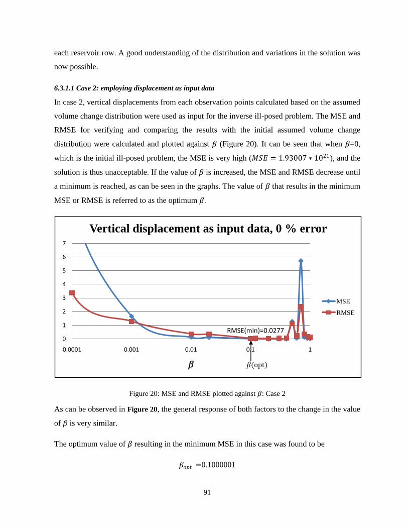
91

each reservoir row. A good understanding of the distribution and variations in the solution was

now possible.

6.3.1.1 Case 2: employing displacement as input data

In case 2, vertical displacements from each observation points calculated based on the assumed

volume change distribution were used as input for the inverse ill-posed problem. The MSE and

RMSE for verifying and comparing the results with the initial assumed volume change

distribution were calculated and plotted against 𝛽 (Figure 20). It can be seen that when 𝛽=0,

which is the initial ill-posed problem, the MSE is very high (𝑀𝑆𝐸 = 1.93007 ∗ 1021), and the

solution is thus unacceptable. If the value of 𝛽 is increased, the MSE and RMSE decrease until

a minimum is reached, as can be seen in the graphs. The value of 𝛽 that results in the minimum

MSE or RMSE is referred to as the optimum 𝛽.

Figure 20: MSE and RMSE plotted against 𝛽: Case 2

As can be observed in Figure 20, the general response of both factors to the change in the value

of 𝛽 is very similar.

The optimum value of 𝛽 resulting in the minimum MSE in this case was found to be

𝛽𝑜𝑝𝑡 =0.1000001

RMSE(min)=0.02770

1

2

3

4

5

6

7

0.0001 0.001 0.01 0.1 1

𝛽

Vertical displacement as input data, 0 % error

MSE

RMSE

𝛽(opt)

92

𝑀𝑆𝐸𝑚𝑖𝑛 = 0.000767697 & 𝑅𝑀𝑆𝐸𝑚𝑖𝑛 = 0.0277073,

For all cases, the results of the back-calculated values for the corner elements of the reservoir

had the greatest error due to the effects of boundary conditions on the calculations. However,

as for the reservoir elements close to the centre, the results had smaller errors and thus were a

better reconstruction than that for the corner elements. Consequently, in each case used for

comparison, this thesis includes the worst cases, which were the corner elements, and the best

reconstruction for each model, which was associated with the centre elements.

The back-calculated results, which were plotted along with the initial distribution of the

volume changes against the reservoir block in each row. The results, shown in Figure 21, were

plotted for the first six rows, which include the worst results, and also for the mid-rows in

Figure 22, which provided the best and closest reconstruction in each model.

93

Figure 21: Δv for the first six rows of the reservoir; Case2.

-0.4

-0.3

-0.2

-0.1

0

0 20 40 60

Val

ue

s

X-direction

Line @ Y = 1

Assumed Calculated

-0.4

-0.3

-0.2

-0.1

0

0 20 40 60

Val

ue

s

X-direction

Line @ Y = 2

Assumed Calculated

-0.4

-0.3

-0.2

-0.1

0

0 20 40 60

Val

ue

s

X-direction

Line @ Y = 3

Assumed Calculated

-0.5

-0.4

-0.3

-0.2

-0.1

0

0 20 40 60

Val

ue

s

X-direction

Line @ Y = 4

Assumed Calculated

-0.5

-0.4

-0.3

-0.2

-0.1

0

0 20 40 60

Val

ue

s

X-direction

Line @ Y = 5

Assumed Calculated

-0.5

-0.4

-0.3

-0.2

-0.1

0

0 20 40 60

Val

ue

s

X-direction

Line @ Y = 6

Assumed Calculated

94

Figure 22: Δv for the rows 25 to 30 of the reservoir; Case2.

-1.2

-1

-0.8

-0.6

-0.4

-0.2

0

0 20 40 60

Val

ue

s

X-direction

Line @ Y = 25

Assumed Calculated

-1.2

-1

-0.8

-0.6

-0.4

-0.2

0

0 20 40 60

Val

ue

s

X-direction

Line @ Y = 26

Assumed Calculated

-1.2

-1

-0.8

-0.6

-0.4

-0.2

0

0 20 40 60

Val

ue

s

X-direction

Line @ Y = 27

Assumed Calculated

-1.2

-1

-0.8

-0.6

-0.4

-0.2

0

0 20 40 60V

alu

es

X-direction

Line @ Y = 28

Assumed Calculated

-1.2

-1

-0.8

-0.6

-0.4

-0.2

0

0 20 40 60

Val

ue

s

X-direction

Line @ Y = 29

Assumed Calculated

-1.2

-1

-0.8

-0.6

-0.4

-0.2

0

0 20 40 60

Val

ue

s

X-direction

Line @ Y = 30

Assumed Calculated

95

6.3.1.2 Case 3: using tilt1 as input data

The same reservoir geometry and observation points used in case 2 were applied in case 3 as

well. The only difference was that for the inverse case, tilt1, which is 𝜕𝑈𝑧

𝜕𝑥 , was used rather than

the vertical displacements as the input data for the back-calculations and the solving of the

inverse case. The results of the MSE and RMSE plotted against 𝛽 can be seen in Figure 23.


As can be seen from a comparison of Figure 20 and Figure 23, the range of 𝛽 that results in an

acceptable resolution is wider when tilt1 is used as input.

The minimum RMSE, and thus the best result, is achieved with 𝛽𝑜𝑝𝑡 = 0.0000004. In this case,

the best result is as follows:

𝑀𝑆𝐸𝑚𝑖𝑛 = 0.000605308, 𝑅𝑀𝑆𝐸𝑚𝑖𝑛 = 0.024603

The resulting volume changes compared to the initial assumed volume changes across each

row in the reservoir for the first six rows and also for rows 25 to 30 are illustrated in Figure 24

and Figure 25.

0

0.2

0.4

0.6

0.8

1

1.2

1.4

1.6

1.8

2

2.2

2.4

1.0E-09 1.0E-07 1.0E-05 1.0E-03 1.0E-01

𝛽

Results with Tilt1 as input, 0 % error

MSE

RMSE

𝛽(opt)

96

Figure 24: Δv for the first six rows; Case 3.

-0.4

-0.3

-0.2

-0.1

0

0 20 40 60

Val

ue

s

X-direction

Line @ Y = 1

Assumed Calculated

-0.4

-0.3

-0.2

-0.1

0

0 20 40 60

Val

ue

s

X-direction

Line @ Y = 2

Assumed Calculated

-0.4

-0.3

-0.2

-0.1

0

0 20 40 60

Val

ue

s

X-direction

Line @ Y = 3

Assumed Calculated

-0.5

-0.4

-0.3

-0.2

-0.1

0

0 20 40 60

Val

ue

s

X-direction

Line @ Y = 4

Assumed Calculated

-0.5

-0.4

-0.3

-0.2

-0.1

0

0 20 40 60

Val

ue

s

X-direction

Line @ Y = 5

Assumed Calculated

-0.5

-0.4

-0.3

-0.2

-0.1

0

0 20 40 60

Val

ue

s

X-direction

Line @ Y = 6

Assumed Calculated

97

Figure 25: Δv for rows 25 to 30 of the reservoir; Case 3.

-1.2

-1

-0.8

-0.6

-0.4

-0.2

0

0 20 40 60

Val

ue

s

X-direction

Line @ Y = 25

Assumed Calculated

-1.2

-1

-0.8

-0.6

-0.4

-0.2

0

0 20 40 60

Val

ue

s

X-direction

Line @ Y = 26

Assumed Calculated

-1.2

-1

-0.8

-0.6

-0.4

-0.2

0

0 20 40 60

Val

ue

s

X-direction

Line @ Y = 27

Assumed Calculated

-1.2

-1

-0.8

-0.6

-0.4

-0.2

0

0 20 40 60

Val

ue

s

X-direction

Line @ Y = 28

Assumed Calculated

-1.2

-1

-0.8

-0.6

-0.4

-0.2

0

0 20 40 60

Val

ue

s

X-direction

Line @ Y = 29

Assumed Calculated

-1.2

-1

-0.8

-0.6

-0.4

-0.2

0

0 20 40 60

Val

ue

s

X-direction

Line @ Y = 30

Assumed Calculated

98

6.3.1.3 Case 4: using tilt2 as input data

The same reservoir geometry and distribution of volume changes and observation points used

in the previous two cases were used in this case as well. The only difference is that tilt2 at each

observation point, which is 𝜕𝑢 𝑧

𝜕𝑦, was used as input for the back-calculations. The results of the

MSE and RMSE plotted against 𝛽 were as shown in Figure 26.


From the graph in Figure 26, it can be determined that the optimum solution occurs at

𝛽𝑜𝑝𝑡 =0.0000003, 𝑀𝑆𝐸𝑚𝑖𝑛 = 0.0005932, 𝑅𝑀𝑆𝐸𝑚𝑖𝑛 = 0.0243557

The graphs of the distribution of the volume changes can be found in Appendix II.

6.3.1.4 Case 5: using tilt1+2

In case 5, a combination of tilt1+2 from each observation point was used as input for the

inverse case. The results obtained are summarized in Figure 27.

0

0.2

0.4

0.6

0.8

1

1.2

1.4

1.6

1.8

2

2.2

2.4

1E-10 1E-08 0.000001 0.0001 0.01 1

𝛽

Results from tilt2 as input, 0 % error

MSE

RMSE

𝛽(opt)

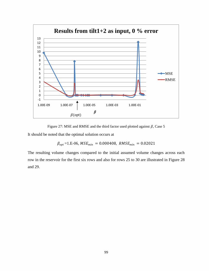
99

Figure 27: MSE and RMSE and the third factor used plotted against 𝛽, Case 5

It should be noted that the optimal solution occurs at

𝛽𝑜𝑝𝑡 =1.E-06, 𝑀𝑆𝐸𝑚𝑖𝑛 = 0.000408, 𝑅𝑀𝑆𝐸𝑚𝑖𝑛 = 0.02021



and 29.

-1

0

1

2

3

4

5

6

7

8

9

10

11

12

13

1.00E-09 1.00E-07 1.00E-05 1.00E-03 1.00E-01

𝛽

Results from tilt1+2 as input, 0 % error

MSE

RMSE

𝛽(opt)

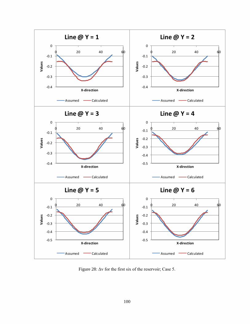
100

Figure 28: Δv for the first six of the reservoir; Case 5.

-0.4

-0.3

-0.2

-0.1

0

0 20 40 60

Val

ue

s

X-direction

Line @ Y = 1

Assumed Calculated

-0.4

-0.3

-0.2

-0.1

0

0 20 40 60

Val

ue

s

X-direction

Line @ Y = 2

Assumed Calculated

-0.4

-0.3

-0.2

-0.1

0

0 20 40 60

Val

ue

s

X-direction

Line @ Y = 3

Assumed Calculated

-0.5

-0.4

-0.3

-0.2

-0.1

0

0 20 40 60

Val

ue

s

X-direction

Line @ Y = 4

Assumed Calculated

-0.5

-0.4

-0.3

-0.2

-0.1

0

0 20 40 60

Val

ue

s

X-direction

Line @ Y = 5

Assumed Calculated

-0.5

-0.4

-0.3

-0.2

-0.1

0

0 20 40 60

Val

ue

s

X-direction

Line @ Y = 6

Assumed Calculated

101

Figure 29: Δv for the rows 25 to 30 of the reservoir; Case 5.

-1.2

-1

-0.8

-0.6

-0.4

-0.2

0

0 20 40 60

Val

ue

s

X-direction

Line @ Y = 25

Assumed Calculated

-1.2

-1

-0.8

-0.6

-0.4

-0.2

0

0 20 40 60

Val

ue

s

X-direction

Line @ Y = 26

Assumed Calculated

-1.2

-1

-0.8

-0.6

-0.4

-0.2

0

0 20 40 60

Val

ue

s

X-direction

Line @ Y = 27

Assumed Calculated

-1.2

-1

-0.8

-0.6

-0.4

-0.2

0

0 20 40 60

Val

ue

s

X-direction

Line @ Y = 28

Assumed Calculated

-1.2

-1

-0.8

-0.6

-0.4

-0.2

0

0 20 40 60

Val

ue

s

X-direction

Line @ Y = 29

Assumed Calculated

-1.2

-1

-0.8

-0.6

-0.4

-0.2

0

0 20 40 60

Val

ue

s

X-direction

Line @ Y = 30

Assumed Calculated

102

6.3.1.5 Case 6 Tilt1+2 + displacements

In case 6, all three sets of data from each observation point were used as input data for solving

the inverse case. The geometry of the reservoir, the number and arrangement of observation

points, and the initial assumed distribution of the volume changes are identical to those of the

previous four cases. The optimum 𝛽 and the minimum RMSE were found to be

𝛽𝑜𝑝𝑡 =0.38, RMSE=0.0208086



and 31.

103

Figure 30: Δv for the first six rows of the reservoir; Case 6.

-0.4

-0.3

-0.2

-0.1

0

0 20 40 60

Val

ue

s

X-direction

Line @ Y = 1

Assumed Calculated

-0.4

-0.3

-0.2

-0.1

0

0 20 40 60

Val

ue

s

X-direction

Line @ Y = 2

Assumed Calculated

-0.4

-0.3

-0.2

-0.1

0

0 20 40 60

Val

ue

s

X-direction

Line @ Y = 3

Assumed Calculated

-0.5

-0.4

-0.3

-0.2

-0.1

0

0 20 40 60V

alu

es

X-direction

Line @ Y = 4

Assumed Calculated

-0.5

-0.4

-0.3

-0.2

-0.1

0

0 20 40 60

Val

ue

s

X-direction

Line @ Y = 5

Assumed Calculated

-0.5

-0.4

-0.3

-0.2

-0.1

0

0 20 40 60

Val

ue

s

X-direction

Line @ Y = 6

Assumed Calculated

104


-1.2

-1

-0.8

-0.6

-0.4

-0.2

0

0 20 40 60

Val

ue

s

X-direction

Line @ Y = 25

Assumed Calculated

-1.2

-1

-0.8

-0.6

-0.4

-0.2

0

0 20 40 60

Val

ue

s

X-direction

Line @ Y = 26

Assumed Calculated

-1.2

-1

-0.8

-0.6

-0.4

-0.2

0

0 20 40 60

Val

ue

s

X-direction

Line @ Y = 27

Assumed Calculated

-1.2

-1

-0.8

-0.6

-0.4

-0.2

0

0 20 40 60

Val

ue

s

X-direction

Line @ Y = 28

Assumed Calculated

-1.2

-1

-0.8

-0.6

-0.4

-0.2

0

0 20 40 60

Val

ue

s

X-direction

Line @ Y = 29

Assumed Calculated

-1.2

-1

-0.8

-0.6

-0.4

-0.2

0

0 20 40 60

Val

ue

s

X-direction

Line @ Y = 30

Assumed Calculated

105

6.3.2 Results of a comparison of cases 2 -- 6

The five cases are identical with respect to the geometry of the reservoir, the distribution of the

volume changes, and the number and distribution of the observation points; the only difference

was the input used for the back-calculation. Table 8 provides a summary and comparison of the

results.

Table 8: Comparison of results from identical cases for which input deformation data varied.

Case No 𝑰𝒏𝒑𝒖𝒕 𝒅𝒂𝒕𝒂 𝒖𝒔𝒆𝒅 𝒘𝒊𝒕𝒉 𝟎 % 𝒆𝒓𝒓𝒐𝒓 𝜷𝑶𝒑𝒕 𝑴𝑺𝑬𝒎𝒊𝒏 𝑹𝑴𝑺𝑬𝒎𝒊𝒏

2 Displacements 0.1000001 0.000767697 0.027707

3 Tilt1 0.0000004 0.0006053 0.024603

4 Tilt2 0.0000003 0.000593 0.024352

5 Tilt1+Tilt2 0.000001 0.000408 0.020199

6 displacements+Tilt1+2 0.38 0.000433 0.020809

Thus, with 0 % error in the input data, which is not a realistic case but rather an ideal case,

using both tilts as input data results in the best resolution. However, it should be noted that

using all three sets of data recorded at each observation point also results in a resolution very

close to that obtained with only two tilts.

As can be seen, although unlike the results expected and contrary to those obtained with

commonly applied techniques, using vertical deformation data for the inverse solution does not

result in the best resolution. Table 8 shows that using observed tilts from each benchmark as

input data for solving the distribution of the volume changes that occur inside a reservoir

results in a much better resolution than using vertical displacements. Moreover, the optimum 𝛽

that results in the best resolution for tilt1 and for tilt 2 is almost identical, and accordingly, the

MSE from the solution of the two cases is almost identical. It can thus be concluded that using

either of the two tilts results in the same resolution with the same optimum 𝛽 and that this

resolution is a much better result than that obtained using displacements as input data as well.

Furthermore, based on Figure 20 and 23, a comparison of the variations in the MSE and RMSE

of the solutions as a function of 𝛽 reveals that the range of 𝛽 that results in an acceptable

resolution is much wider when tilt1 is used as input than when vertical displacements are used.

106

6.4 Limiting the area range for observation points using tilts

As mentioned previously, it has been shown that a volume change that occurs in the subsurface

at depth d would affect and cause displacement and surface deformations mostly in an area

with a radius of d around the centre of the subsurface deformation. Thus, to be able to back-

calculate and reconstruct the initial volume, data from all areas affected should be gathered and

employed for the back-calculation. In other words, observation points are best chosen

throughout the entire area affected by the volume change, in order to enable the reconstruction

of the actual value of the volume change. However, in actual reservoir cases, the reservoir

itself is a huge body, and the area affected by a change in volume in the subsurface is

manifested in a larger area at ground level. As well, oil reservoirs are usually located at

substantial depths, thus affecting an even wider range of area at the surface level. It might not

be convenient to choose benchmarks over the very vast area that is affected and deformed

because there might be limitations caused by the presence of structures or other natural

barriers. It is thus of interest to determine whether using tilts as input data for back-calculations

will allow the limitation of the area of measurements and the investigation of the possibility of

omitting some of the data points, while still resulting in the reconstruction of the initial volume

change with an acceptable degree of accuracy.

6.4.1 Case 7

In case 7, the geometry of the reservoir and initial distribution of the volume changes are

identical to those in the previous cases. The number of observation points is also the same:

2704. The only difference incorporated is that the points were chosen from a limited area:

−5 ≤ 𝑋𝑜𝑏𝑠𝑒𝑟 , 𝑌𝑜𝑏𝑠𝑒𝑟 ≤ 505

The area chosen for the observation grid, as shown in Figure 32 is located directly above the

area of the reservoir (the area indicated by hatch marks).

107

Figure 32: Cutting out a part of data by limiting the observation area on the surface and thus using only

data from part of the observation field

Tilt 1 and tilt2 at each observation point were used separately as input data for the back-

calculations. The results for these two cases are summarized in Table 9.

500

500

1500

Deformation Field on the Surface

108

Table 9: MSE and RMSE for different 𝛽s: tilt1 and tilt2

Results from tilt1

Results from tilt2

𝛽 MSE RMSE

𝛽 MSE RMSE

0 1.35E+21 3.67E+10

0 2.19E+21 4.68E+10

1E-09 16.5416 4.06714

1.00E-09 44.4929 6.6703

1E-08 0.794137 0.891143

1.00E-08 1.61051 1.26906

1E-08 0.874255 0.935016

1.00E-07 0.539316 0.734381

1.01E-08 0.707968 0.841408

0.000001 0.001949 0.044149

1.02E-08 1.78159 1.33476

0.00001 0.00506 0.071132

1.1E-08 0.972188 0.985996

0.0001 0.001314 0.036246

2E-08 0.750146 0.86611

0.001 0.002542 0.050415

3E-08 0.214924 0.463599

0.01 0.015098 0.122873

4E-08 0.0562546 0.237181

0.1 88.4328 9.40387

4.01E-08 0.24359 493548

0.2 0.186553 0.431918

4.1E-08 0.110251 0.332041

4.2E-08 0.714769 0.84544

5E-08 1.77428 1.33202

1E-07 1.00122 1.00061

0.000001 0.005576 0.074673

0.00001 0.0046435 0.068144

0.0001 0.0013079 0.036164

0.001 0.0027544 0.052483

0.01 0.0300482 0.173344

0.1 73.4291 8.56908

0.2 0.1891 0.434856

1 0.0758763 0.275457

It can be observed from Table 9 that the results from tilts 1 and 2 are very similar, meaning that

the optimum 𝛽 in both cases is the same, as is the minimum MSE or RMSE.

As can be seen, the RMSE is small. Plots of the volume changes calculated based on tilt2 as

input, along with the initial assumed volume changes are summarized in one graph, for the first

five rows of the reservoir (Figure 33).

109

Figure 33: Volume changes in volume in the first five rows of the reservoir, with the observation field

limited

Table 10 provides a summary and comparison of the results of case 7 and case 4, which is a

similar case but with observation points scattered over an area of −500 ≤ 𝑋, 𝑌 ≤ 1000.

Table 10: Comparison of results for a limited area of observation points

case range of observation points MSE RMSE

4 -500<X,Y<1000 0.000593 0.024351591

7 -5<X,Y<505 0.001314 0.0362455

As expected, the results from case 4 are better, and the RMSE of the calculated results is lower

because the input data used in case 4 are taken from the entire deformation field. However, an

examination of the plots of the calculated volumes and the initial assumed volume changes

(Figure 33) shows that case 7 also results in an acceptable resolution. Therefore if tilts are used

as input data, the area of observation can be limited, which would be more convenient for

obtaining experimental observation data.

-1.6-1.5-1.4-1.3-1.2-1.1

-1-0.9-0.8-0.7-0.6-0.5-0.4-0.3-0.2-0.1

0

0 20 40 60V

olu

me

cha

ng

e

Reservoir section

Limiting area of observation-tilt2 as

input

Row1-initial

Row1-calculated

Row2-initial

Row2-calculated

Row3-initial

Row3-calculated

Row4-initial

Row4-calculated

Row5-initial

Row5-calculated

110

6.5 Error in the input data

In the cases studied, it was assumed that the observation data recorded from the observation

points does not contain errors and that the values recorded are the exact actual values of

deformations caused due to the volume change occurring in the reservoir. In reality, however,

error is always present in recorded experimental data. Consequently, an engineer cannot expect

to have precise measurements of deformations. This section presents the effect of the error

present in the measurements of the displacements and tilts, which are used as input for the

inverse case, on the resolution of the ill-posed problem. A random number generator was used

to generate random errors within a given range. With respect to the maximum of the random

error generated, a percentage of the maximum observation data gathered from the entire

observation grid was used to render the results more practical and applicable for general cases.

Thus, based on a percentage of the maximum amount of observation data recorded, the

maximum error that would not affect the results to a significant extent is to be found. This

random error was then added to each observation data point used as input for the back-

calculations. For example, if vertical displacement is used as input, a random error that is 10%

of the maximum value of the vertical displacement is incorporated, as follows:

0 ≤ 𝑅𝑎𝑛𝑑𝑜𝑚 𝑒𝑟𝑟𝑜𝑟

≤ 𝑚𝑎𝑥𝑖𝑚𝑢𝑚 𝑣𝑎𝑙𝑢𝑒 𝑜𝑓 𝑑𝑖𝑠𝑝𝑙𝑎𝑐𝑒𝑚𝑒𝑛𝑡 𝑟𝑒𝑐𝑜𝑟𝑑𝑒𝑑 𝑖𝑛 𝑜𝑏𝑠𝑒𝑟𝑣𝑎𝑡𝑖𝑜𝑛 𝑝𝑜𝑖𝑛𝑡𝑠

∗ 10%

𝑑𝑠𝑖𝑝𝑙𝑎𝑐𝑒𝑚𝑒𝑛𝑡𝑒𝑟𝑟𝑜𝑟 𝑖= 𝑑𝑖𝑠𝑝𝑙𝑎𝑐𝑒𝑚𝑒𝑛𝑡𝑖 + 𝑅𝑎𝑛𝑑𝑜𝑚 𝑒𝑟𝑟𝑜𝑟

Thus, 𝑑𝑠𝑖𝑝𝑙𝑎𝑐𝑒𝑚𝑒𝑛𝑡𝑒𝑟𝑟𝑜𝑟 𝑖 is substituted as input data for the back-calculations.

6.5.1 The effect of the error present in vertical displacement measurements on the resolution of

the ill-posed problem

For these cases, the geometry of the reservoir, the distribution of volume changes and the

observation points are all identical to those of the previous cases.

6.5.1.1 Case 8: random error of 0-1 mm, which is 0.55 % of the maximum value recorded

The maximum displacement calculated due to the assumed distribution of the volume changes

was found to be

111

𝑑𝑖𝑠𝑝𝑙𝑎𝑐𝑒𝑚𝑒𝑛𝑡𝑚𝑎𝑥 = 0.182285 𝑚

Therefore, for the first case, a random error with the following range was generated:

0 ≤ 𝑟𝑎𝑛𝑑𝑜𝑚 𝑒𝑟𝑟𝑜𝑟 ≤ 1𝑚𝑚

This amount of error would be 0.5486 % of the maximum displacement value measured. This

error was added to the displacements calculated for each observation point, and the resulting

value then was used as input for the back-calculations.


The optimum 𝛽 resulting in the minimum MSE in this case was 𝛽=0.2, 𝑀𝑆𝐸𝑚𝑖𝑛 =0.141099



and 36.

-1

1

3

5

7

9

11

13

15

17

19

21

23

25

0.0001 0.001 0.01 0.1 1

𝛽

Displacement with 0<error<1 mm

MSE

RMSE

𝛽(opt)

112


-0.8

-0.6

-0.4

-0.2

0

0 20 40 60

Val

ue

s

X-direction

Line @ Y = 1

Assumed Calculated

-0.8

-0.6

-0.4

-0.2

0

0 20 40 60

Val

ue

s

X-direction

Line @ Y = 2

Assumed Calculated

-0.8

-0.6

-0.4

-0.2

0

0 20 40 60

Val

ue

s

X-direction

Line @ Y = 3

Assumed Calculated

-0.8

-0.6

-0.4

-0.2

0

0 20 40 60

Val

ue

s

X-direction

Line @ Y = 4

Assumed Calculated

-0.6

-0.5

-0.4

-0.3

-0.2

-0.1

0

0 20 40 60

Val

ue

s

X-direction

Line @ Y = 5

Assumed Calculated

-0.6

-0.5

-0.4

-0.3

-0.2

-0.1

0

0 20 40 60

Val

ue

s

X-direction

Line @ Y = 6

Assumed Calculated

113


-2.5

-2

-1.5

-1

-0.5

0

0 20 40 60

Val

ue

s

X-direction

Line @ Y = 25

Assumed Calculated

-2.5

-2

-1.5

-1

-0.5

0

0 20 40 60

Val

ue

s

X-direction

Line @ Y = 26

Assumed Calculated

-2.5

-2

-1.5

-1

-0.5

0

0 20 40 60

Val

ue

s

X-direction

Line @ Y = 27

Assumed Calculated

-2.5

-2

-1.5

-1

-0.5

0

0 20 40 60

Val

ue

s

X-direction

Line @ Y = 28

Assumed Calculated

-2

-1.5

-1

-0.5

0

0 20 40 60

Val

ue

s

X-direction

Line @ Y = 29

Assumed Calculated

-2

-1.5

-1

-0.5

0

0 20 40 60

Val

ue

s

X-direction

Line @ Y = 30

Assumed Calculated

114

As can be seen, adding only 0.5486 % of the maximum displacement value as error would

completely change the results both in the shape of the volume distribution and also the

magnitude of the values calculated. Displacements at observation points are therefore not

suitable input data for solving the inverse ill-posed problem.

6.5.2 The effect of the error present in tilt measurements on the resolution of the ill-posed

problem

6.5.2.1 Case 9: tilts1+2 with 3 % error

The geometry of the reservoir and the initial distribution of the volume changes are identical to

those in the previous cases. With respect to the observation points, the entire deformation field

considered was −500 ≤ 𝑥, 𝑦 ≤ 1000. Tilts1+2 from each observation point were used as input

data. As shown in previous sections, tilts1+2 result in the best resolution. The maximum value

of the tilt in the deformation field was calculated to be

𝑡𝑖𝑙𝑡𝑚𝑎𝑥 = 3.73 ∗ 10−4

A value for random error was introduced in the following manner:

0 ≤ 𝑒𝑟𝑟𝑜𝑟 ≤ 3% ∗ 𝑡𝑖𝑙𝑡𝑚𝑎𝑥

This random error was then added to each data set from each observation point

𝑡𝑖𝑙𝑡1𝑖 𝑒𝑟𝑟𝑜𝑟= 𝑟𝑎𝑛𝑑𝑜𝑚 𝑒𝑟𝑟𝑜𝑟 + 𝑡𝑖𝑙𝑡1𝑖

𝑡𝑖𝑙𝑡2𝑖 𝑒𝑟𝑟𝑜𝑟= 𝑟𝑎𝑛𝑑𝑜𝑚 𝑒𝑟𝑟𝑜𝑟 + 𝑡𝑖𝑙𝑡2𝑖

These data were then used as input for the back-calculations. The volume changes calculated

were plotted along with the initial assumed volume changes and are shown in Appendix III.

6.5.2.2 Case 10: tilts1+2 with 6 % error

In case 10, 6 % of the maximum value of the tilts was added as the random error. The changes

in volume calculated were plotted along with the initial assumed changes in volume and are

shown in Appendix III.

115

6.5.2.3 Case 11: Tilts1+2 with 9 % error

The volume changes calculated were plotted along with the initial assumed changes in volume

and are shown in Appendix III.

Case 12, using 10% error; case 13, using 12% error; case 14, using 15% error; case15, using

15% error, and case16, using 20% error were also modeled. The results from these cases are

summarized in Figure 37.

Figure 37: Results of RMSE from the inverse solution of different cases using tilt1+tilt2 with error

plotted against 𝛽.

As can be seen, increasing the error results in an increase in the minimum standard deviation,

and the general trend is almost identical in all cases. The solutions thus deviate farther from the

exact solution.

00.010.020.030.040.050.060.070.080.09

0.10.110.120.130.140.150.160.170.180.19

0.2

0 0.01 0.02 0.03 0.04 0.05 0.06 0.07 0.08

𝛽

RMSE versus 𝛽

RMSE-3%

RMSE-6%

RMSE-9%

RMSE-10%

RMSE-12%

RMSE-15%

RMSE-17%

RMSE-20%

116

The above chart can be summarized in Table 11.

Table 11: Minimum MSE for different error percentages used as input

Tilt1+tilt2 used as input data

Case

% error of the

maximum tilt

value added

𝑴𝑺𝑬𝒎𝒊𝒏 𝑹𝑴𝑺𝑬𝒎𝒊𝒏

9 3% 0.005156 0.071804

10 6% 0.006081 0.07798

11 9% 0.007841 0.088552

12 10% 0.008614 0.092814

13 12% 0.010438 0.102166

14 15% 0.008614 0.092814

15 17% 0.016622 0.128927

16 20% 0.021447 0.146448



and 39.

117


-1

-0.8

-0.6

-0.4

-0.2

0

0.2

0.4

0 20 40 60

Val

ue

s

X-direction

Line @ Y = 1

Assumed Calculated

-1

-0.8

-0.6

-0.4

-0.2

0

0.2

0.4

0 20 40 60

Val

ue

s

X-direction

Line @ Y = 2

Assumed Calculated

-1

-0.8

-0.6

-0.4

-0.2

0

0.2

0.4

0 20 40 60

Val

ue

s

X-direction

Line @ Y = 3

Assumed Calculated

-1

-0.8

-0.6

-0.4

-0.2

0

0.2

0.4

0 20 40 60V

alu

es

X-direction

Line @ Y = 4

Assumed Calculated

-1

-0.8

-0.6

-0.4

-0.2

0

0.2

0.4

0 20 40 60

Val

ue

s

X-direction

Line @ Y = 5

Assumed Calculated

-1

-0.8

-0.6

-0.4

-0.2

0

0.2

0.4

0 20 40 60

Val

ue

s

X-direction

Line @ Y = 6

Assumed Calculated

118


-1.2

-1

-0.8

-0.6

-0.4

-0.2

0

0 20 40 60

Val

ue

s

X-direction

Line @ Y = 25

Assumed Calculated

-1.2

-1

-0.8

-0.6

-0.4

-0.2

0

0 20 40 60

Val

ue

s

X-direction

Line @ Y = 26

Assumed Calculated

-1.2

-1

-0.8

-0.6

-0.4

-0.2

0

0 20 40 60

Val

ue

s

X-direction

Line @ Y = 27

Assumed Calculated

-1.2

-1

-0.8

-0.6

-0.4

-0.2

0

0 20 40 60

Val

ue

s

X-direction

Line @ Y = 28

Assumed Calculated

-1.2

-1

-0.8

-0.6

-0.4

-0.2

0

0 20 40 60

Val

ue

s

X-direction

Line @ Y = 29

Assumed Calculated

-1.2

-1

-0.8

-0.6

-0.4

-0.2

0

0 20 40 60

Val

ue

s

X-direction

Line @ Y = 30

Assumed Calculated

119

From the above charts, it can be seen that using tilts1+2 as input data for the back-calculations,

even when up to 20 % of the maximum value of recorded tilts is incorporated as error, would

result in a volume change distribution calculated close to what expected with a good resolution.

6.5.3 The effect of error present in vertical displacement + tilts1+2 on the resolution of the ill-

posed problem

6.5.3.1 Case 17: using vertical displacement + tilts1+2 with 1 % error present in all three sets of data

The geometry of the reservoir, volume change distribution and the total number of observation

points are the same as those in the previous cases. The observation grid is extended over the

reservoir to include the following range:

−500 ≤ 𝑋𝑜𝑏𝑠𝑒𝑟 , 𝑌𝑜𝑏𝑠𝑒𝑟 ≤ 1000

With respect to the input for the back-calculations, tilts1+2 + the vertical displacement from

each observation point were used. To enable all the data to be used together, as mentioned in

the previous section, the values were normalized and then divided by the maximum value in

the data set so that all three sets of data would be in the same range. With respect to the error,

only 1 % of the maximum value was considered as random error, and the procedure used is as

follows:

0 ≤ 𝑟𝑎𝑛𝑑𝑜𝑚 𝑒𝑟𝑟𝑜𝑟𝑡𝑖𝑙𝑡 ≤ 1% ∗ 𝑡𝑖𝑙𝑡𝑚𝑎𝑥

0 ≤ 𝑟𝑎𝑛𝑑𝑜𝑚 𝑒𝑟𝑟𝑜𝑟𝑑𝑖𝑠𝑝𝑙𝑎𝑐𝑒𝑚𝑒𝑛𝑡 ≤ 1% ∗ 𝑑𝑖𝑠𝑝𝑙𝑎𝑐𝑒𝑚𝑒𝑛𝑡𝑚𝑎𝑥

𝑇𝑖𝑙𝑡1𝑒𝑟𝑟𝑜𝑟 𝑖= 𝑅𝑎𝑛𝑑𝑜𝑚 𝑒𝑟𝑟𝑜𝑟𝑡𝑖𝑙𝑡 1 + 𝑡𝑖𝑙𝑡1𝑖

𝑇𝑖𝑙𝑡2𝑒𝑟𝑟𝑜𝑟 𝑖= 𝑅𝑎𝑛𝑑𝑜𝑚 𝑒𝑟𝑟𝑜𝑟𝑡𝑖𝑙𝑡 2 + 𝑡𝑖𝑙𝑡2𝑖

𝑑𝑖𝑠𝑝𝑙𝑎𝑐𝑒𝑚𝑒𝑛𝑡𝑒𝑟𝑟𝑜𝑟 𝑖= 𝑅𝑎𝑛𝑑𝑜𝑚 𝑒𝑟𝑟𝑜𝑟𝑑𝑖𝑠𝑝𝑙𝑎𝑐𝑒𝑚𝑒𝑛𝑡 + 𝑑𝑖𝑠𝑝𝑙𝑎𝑐𝑒𝑚𝑒𝑛𝑡𝑖

For the back-calculations, these data incorporating the error were used as the input data from

each observation point. The results are shown in Figure 40.

120


The following should be noted: βopt =0.5, MSEmin = 0.501324, RMSEmin =0.708043. The

resulting volume changes compared to the initial assumed volume changes across each row in

the reservoir for the first six rows and also for rows 25 to 30 are illustrated in Figure 41 and 42.

-1

0

1

2

3

4

5

6

0.3 0.4 0.5 0.6 0.7 0.8 0.9 1 1.1

𝛽

Displacement + tilts1+ 2, with 1% error

MSE

RMSE

𝛽(opt)

121


-1.2

-1

-0.8

-0.6

-0.4

-0.2

0

0 20 40 60

Val

ue

s

X-direction

Line @ Y = 1

Assumed Calculated

-1.2

-1

-0.8

-0.6

-0.4

-0.2

0

0 20 40 60

Val

ue

s

X-direction

Line @ Y = 2

Assumed Calculated

-1.2

-1

-0.8

-0.6

-0.4

-0.2

0

0 20 40 60

Val

ue

s

X-direction

Line @ Y = 3

Assumed Calculated

-1

-0.8

-0.6

-0.4

-0.2

0

0 20 40 60

Val

ue

s

X-direction

Line @ Y = 4

Assumed Calculated

-1

-0.8

-0.6

-0.4

-0.2

0

0 20 40 60

Val

ue

s

X-direction

Line @ Y = 5

Assumed Calculated

-0.8

-0.6

-0.4

-0.2

0

0 20 40 60

Val

ue

s

X-direction

Line @ Y = 6

Assumed Calculated

122


-4

-3

-2

-1

0

1

0 20 40 60

Val

ue

s

X-direction

Line @ Y = 25

Assumed Calculated

-4

-3

-2

-1

0

1

0 20 40 60

Val

ue

s

X-direction

Line @ Y = 26

Assumed Calculated

-4

-3

-2

-1

0

1

0 20 40 60

Val

ue

s

X-direction

Line @ Y = 27

Assumed Calculated

-4

-3

-2

-1

0

1

0 20 40 60V

alu

es

X-direction

Line @ Y = 28

Assumed Calculated

-4

-3

-2

-1

0

1

0 20 40 60

Val

ue

s

X-direction

Line @ Y = 29

Assumed Calculated

-3

-2

-1

0

1

0 20 40 60

Val

ue

s

X-direction

Line @ Y = 30

Assumed Calculated

123

As can be seen, adding only 1 % of the maximum values as error significantly affects the

solution; the volume change distribution and the associated values are not at all close to the

initial assumed distributions and values.

Table 12 summarizes the effect of error present in the observation data taken from the surface

deformation field on the solution of the inverse problem and the resulting back-calculated

volume change distributions.

Table 12: Results summarized to show the effect of error in the observation data.

Case input data %

error 𝜷𝑶𝒑𝒕 𝑴𝑺𝑬𝒎𝒊𝒏 𝑹𝑴𝑺𝑬𝒎𝒊𝒏

2 displacement 0% 0.1000001 0.000768 0.027707

8 displacement 0.55% 0.2 0.141099 0.375631

6 displacements+Tilt1+2 0% 0.38 0.000433 0.020809

5 Tilt1+Tilt2 0% 0.000001 0.000408 0.020199

9 Tilt1+Tilt2 3% 0.02 0.005156 0.071804

10 Tilt1+Tilt2 6% 0.02 0.006081 0.07798

11 Tilt1+Tilt2 9% 0.02 0.007841 0.088552

12 Tilt1+Tilt2 10% 0.02 0.008614 0.092814

13 Tilt1+Tilt2 12% 0.02 0.010438 0.102166

14 Tilt1+Tilt2 15% 0.02 0.008614 0.092814

15 Tilt1+Tilt2 17% 0.02 0.016622 0.128927

16 Tilt1+Tilt2 20% 0.02 0.021447 0.146448

17 displacements+Tilt1+2 1% 0.5 0.501324 0.708043

6.6 Effect of the number of observation points on the inverse resolution

The number of observation points is another important factor in every monitoring and

controlling project. The higher the number of observation points, the more devices must be

used for observing and recording data, which for this study is the displacement data and tilts.

Moreover, more time and energy would be required for the installation, monitoring and

maintenance of the additional devices. On the other hand, the more observation points that are

used, the more data that can be acquired from the deformation field, which would result in

better resolution. Determining the optimum number of observation points would therefore be

helpful for obtaining the desired resolution economically.

124

For the cases described so far, 2704 benchmarks were used, which is, in fact, an impractical

number of observation points and would never actually be used. The number was chosen for

the previous cases based on the number of reservoir elements. The reservoir was divided into

grids with 50*50 elements, or 2500 overall. Thus the number of unknown volume changes to

be solved for from the inverse case in this case was 2500. Based on that number, 2704

observation points were used, and the number of available data sets or known parameters was

thus 2704. To study the sensitivity of the resolution to the number of observation points, some

observation points were randomly omitted for each case. The percentage of the points omitted

was based on the number of unknowns to be solved for, or the reservoir elements: 2500. This

method was used in order to generalize the problem and so that the results would be applicable

to a variety of cases.

To determine the sensitivity of the calculations to the number of observation points, the general

model used in the previous cases with the same geometry and initial volume change

distribution was applied here as well. The following cases were studied:

6.6.1 Omitting random points using tilt1+ 2 + displacement with 0 % error as input

All three data sets from each observation point, assuming that the data contains 0 % error and

that the values are the exact actual values, were used as input for the cases presented in this

section.

6.6.1.1 Case 18: omitting 4 % of the observation points

For case 18, 96 % of the number of reservoir elements, or 2400 points, were used as

observation points. The MSE and RMSE plotted against 𝛽 for the results are shown in Figure

43.

𝛽𝑜𝑝𝑡 = 0.54, 𝑀𝑆𝐸 = 0.000547, RMSE = 0.023385

125

Figure 43: MSE and RMSE plotted against 𝛽: Case 18.

6.6.1.2 Case 19

In case 19, 90 % of the unknowns were used as the number of observation points. The results

for 2250 observation points are shown in Figure 44.

𝛽𝑜𝑝𝑡 = 0.37, 𝑀𝑆𝐸 =0.000579, RMSE = 0.024057


-0.5

0

0.5

1

1.5

2

2.5

3

0 0.2 0.4 0.6 0.8 1

𝛽

Tilts1+2 + displacement with 0%

error

MSE

RMSE

-0.5

0

0.5

1

1.5

2

2.5

3

0 0.2 0.4 0.6 0.8 1

𝛽

Tilts1+2 + displacement , with 0 %

error, omitting 10 % of the points

MSE

RMSE

𝛽(opt)

𝛽𝑜𝑝𝑡

126

6.6.1.3 Case 20

For case 20, 20% of the total number of elements were randomly omitted from the

benchmarks. Thus the calculations were performed using 2000 observation points. The results

can be seen in Figure 45.

𝛽𝑜𝑝𝑡 = 0.38, 𝑀𝑆𝐸 = 0.000601, RMSE = 0.024514


6.6.1.4 Case 21

For case 21, 40% *2500 of the observation points were randomly omitted, and the results using

1500 points, as shown in Figure 46, were calculated as follows:

𝛽𝑜𝑝𝑡 = 0.2, 𝑀𝑆𝐸 = 0.000844, RMSE = 0.029051

-0.5

0

0.5

1

1.5

2

2.5

3

0 0.2 0.4 0.6 0.8 1

𝛽

Tilts1+2 + displacement, omitting

20% of the points

MSE

RMSE

𝛽(opt)

127


6.6.1.5 Case 22

For case 22, 60%*2500 of the observation points were randomly omitted. Using 1000 points,

the results of the MSE and RMSE were plotted against 𝛽, as shown in Figure 47, were as

follows:

𝛽𝑜𝑝𝑡 = 0.22, 𝑀𝑆𝐸 = 0.000703, RMSE = 0.026517


-0.1

0

0.1

0.2

0.3

0.4

0.5

0.6

0 0.1 0.2 0.3 0.4 0.5 0.6

𝛽


40 % of the points

MSE

RMSE

𝛽(opt)

0

0.01

0.02

0.03

0.04

0.05

0.06

0 0.1 0.2 0.3 0.4 0.5 0.6

𝛽


60 % of the points

MSE

RMSE

𝛽(opt)

128

6.6.1.6 Case 23

For case 23, 80%*2500 of the data points were randomly omitted, and 500 random points were

used. The results of MSE and RMSE plotted against 𝛽 were as shown in Figure 48.

𝛽𝑜𝑝𝑡 = 0.1, 𝑀𝑆𝐸 = 0.000666, RMSE = 0.025801


6.6.1.7 Case 24

For case 24, when 90%*2500 of the observation points were omitted, 250 points were used.

The resulting MSE and RMSE were plotted against, as shown in Figure 49.

𝛽𝑜𝑝𝑡 = 0.78, 𝑀𝑆𝐸 = 0.001742, RMSE = 0.041741

-0.05

0

0.05

0.1

0.15

0 0.1 0.2 0.3 0.4 0.5 0.6

𝛽


80 % of the points

MSE

RMSE

𝛽(opt)

129


6.6.1.8 Case 25

For case 25, 96%*2500 of the observation points were randomly deleted, and 100 points were

used as observation points. The results were as shown in Figure 50.

𝛽𝑜𝑝𝑡 = 0.78, 𝑀𝑆𝐸 = 0.001742, RMSE = 0.041741

0

0.05

0.1

0.15

0.2

0 0.2 0.4 0.6 0.8 1

𝛽


90% of the points

MSE

RMSE

𝛽(opt)

130


6.6.1.9 Case 26

For case 26, about 98% of the observation points were omitted, and 50 points were used as

observation points. The results can be seen in Figure 51.

𝛽𝑜𝑝𝑡 = 0.3, 𝑀𝑆𝐸 = 0.001764, RMSE = 0.042006

0

0.01

0.02

0.03

0.04

0.05

0.06

0.07

0.08

0 0.2 0.4 0.6 0.8 1

𝛽


96% of the points

MSE

RMSE

𝛽(opt)

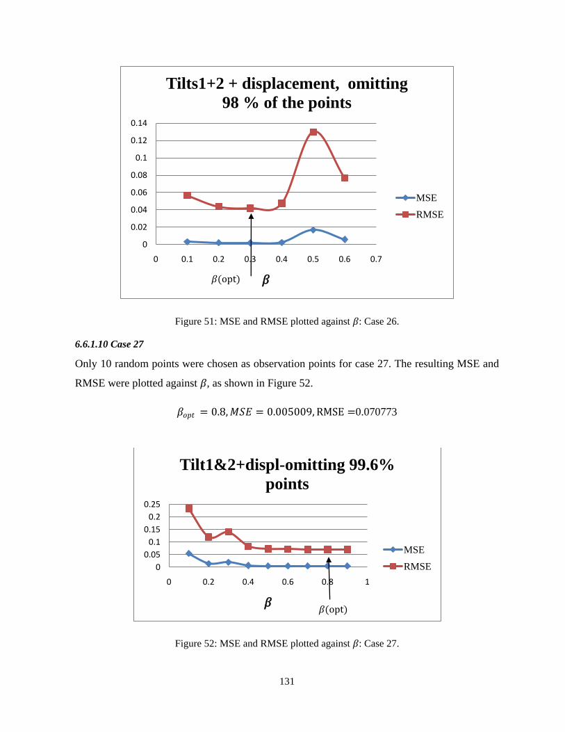
131


6.6.1.10 Case 27

Only 10 random points were chosen as observation points for case 27. The resulting MSE and

RMSE were plotted against 𝛽, as shown in Figure 52.

𝛽𝑜𝑝𝑡 = 0.8, 𝑀𝑆𝐸 = 0.005009, RMSE =0.070773


0

0.02

0.04

0.06

0.08

0.1

0.12

0.14

0 0.1 0.2 0.3 0.4 0.5 0.6 0.7

𝛽


98 % of the points

MSE

RMSE

𝛽(opt)

0

0.05

0.1

0.15

0.2

0.25

0 0.2 0.4 0.6 0.8 1

𝛽

Tilt1&2+displ-omitting 99.6%

points

MSE

RMSE

𝛽(opt)

132

Table 13 provides a summary and comparison of the results of the above cases, and Figure 53

shows the RMSE plotted against the number of observation points used.

Table 13: Comparison of results to show the effect of the number of observation points.

Case Data used for input %

error

Number of

observation

points used

% of the

initial

observation

points

randomly

omitted

𝜷 𝑶𝒑𝒕 𝑴𝑺𝑬𝒎𝒊𝒏 𝑹𝑴𝑺𝑬𝒎𝒊𝒏

6 tilt1+2+displacement 0% 2704 0% 0.38 0.000433 0.020809










27 tilt1+2+displacement 0% 10 99.60% 0.8 0.005009 0.070773

28 tilt1+2+displacement 0% 1 99.96% 0.12 0.05674 0.238201

Figure 53: RMSE plotted against the number of observation points.

0

0.1

0.2

0.3

1 10 100 1000 10000

RM

SE

Number of observation points

RMSE versus number of observation

points

133

The results of the volume change calculations in each case, along with the initial assigned

volume changes, were plotted in graphs for each block of the reservoir. The graphs are

provided in Appendix IV.

As expected, it can be seen that omitting more points and thus using a lower number of

observation benchmarks generally causes the RMSE to increase, which translates into a less

accurate solution. However, from the graphs plotted and included in Appendix IV, it can be

seen that if the error in the observation data is assumed to be 0, using only 10 points, or 99.6%

of the number of reservoir elements, and thus having only 10 known data would result in an

acceptable resolution. A closer examination of the results of the cases presented in Table 13

reveals that the RMSE does not change significantly with the omission of a large number of

observation points, and thus a large amount of data. Using 2400 points resulted in a MSE of

0.000547 whereas, when 1900 points were omitted and only 500 used, the MSE increased only

to 0.000666. Therefore, using a large number of benchmarks does not necessarily mean a much

better resolution when a combination of tilts is used as input data. Thus, the resolution is not

very sensitive to the number of observation points if the error in the observed data is

considered to be zero.

From Table 13, it can be seen that for cases 22 and 23, omitting observation points leads to a

slight decrease in the MSE. This effect could be due to the use of random points as observation

data; thus, although the number of points used in these cases is lower, the composition of the

grid of these points has a better distribution, and thus, the data gathered results in better

resolution. The following sections present an examination of the effect of the distribution of the

observation points on the resolution.

6.7 The effect of the distribution of the observation points on the resolution of the

inverse problem

In the above cases, it was seen that the number of observation points does not need to be equal

to the number of reservoir elements, which is the number of unknowns, and points can thus be

omitted. However, for the above cases the points were randomly chosen for omission. In actual

cases, however, it is practical to have a specific routine for choosing the distribution of the

benchmarks because the observation process would be more convenient and easier to install,

observe, and monitor. Moreover, the most important point is that the deformation field can be

134

reconstructed more effectively if an appropriate pattern is chosen for the distribution of the

benchmarks.

To observe the sensitivity of the inverse case resolution to the distribution of the benchmarks

chosen for collecting data on the surface above the reservoir, a number of cases scenarios were

studied, and the results are presented in this section.

6.7.1 0% error present in the observation data

Data for tilts1+2 + displacements were used as input for the following cases, meaning that all

three data sets from each observation point were used. A 0% error was assumed for the input

data, and thus the exact calculated displacements and tilts were used for the calculations. The

geometry of the reservoir and the initial volume change distribution were the same as in the

previous cases. The number of observation points used was 100.

6.7.1.1 Case 29

The 100 benchmarks for case 29 were distributed in two rows, one vertical and one horizontal,

that meet at a corner directly above the reservoir:

𝑋𝑜𝑏𝑠𝑒𝑟 = 5

5 ≤ 𝑌𝑜𝑏𝑠𝑒𝑟 ≤ 495

and 𝑌𝑜𝑏𝑠𝑒𝑟 = 5

5 ≤ 𝑋𝑜𝑏𝑠𝑒𝑟 ≤ 495

The plan of the observation points placed above the reservoir is shown in the Figure 54. As can

be seen, two rows of observation points, with 50 points in each row, are shown as crosses in

two outside reservoir element rows that meet at a corner.

135

Figure 54: Plan of reservoir with observation points distributed in two rows, one vertical and one

horizontal, which meet at the corner above the reservoir.

The resulting MSE and RMSE plotted against 𝛽 were as shown in Figure 55.

𝛽𝑜𝑝𝑡 = 0.1, 𝑀𝑆𝐸 = 0.0024587, RMSE =0.04958528

Figure 55: MSE and RMSE for different values of 𝛽s: Case 29

6.7.1.2 Case 30

For case 30, the 100 observation points were distributed in two rows, one vertical and one

horizontal, which cross above the mid-point of the reservoir:

-1

1

3

5

7

9

0.00001 0.0001 0.001 0.01 0.1 1

𝛽

Tilts1+2 + displacement, with 0 % error

MSE

RMSE

(𝛽opt)

136


5 ≤ 𝑌𝑜𝑏𝑠𝑒𝑟 ≤ 495

And 𝑌𝑜𝑏𝑠𝑒𝑟 = 250

5 ≤ 𝑋𝑜𝑏𝑠𝑒𝑟 ≤ 495

The plan of the observation points placed above the reservoir is shown in Figure 56.

Figure 56: Plan of reservoir with observation points distributed in two rows, one horizontal and one

vertical, which cross at the centre of the reservoir.

The results of MSE and RMSE plotted against 𝛽 were as shown in Figure 57.

𝛽𝑜𝑝𝑡 = 0.6, 𝑀𝑆𝐸 = 0.0017898, RMSE =0.042306028


0

0.02

0.04

0.06

0.08

0.1

0.12

0.14

0 0.2 0.4 0.6 0.8 1

𝛽

Tilts1+2 + displacement, with 0 % error

MSE

RMSE

(𝛽opt)

137

6.7.1.3 Case31:

In case 31, the 100 points extend from -500 to 1000, in two rows placed at the centre of the

reservoir:


−500 ≤ 𝑌𝑜𝑏𝑠𝑒𝑟 ≤ 1000

And 𝑌𝑜𝑏𝑠𝑒𝑟 = 250

−500 ≤ 𝑋𝑜𝑏𝑠𝑒𝑟 ≤ 1000

The results were as shown in Figure 58.

𝛽𝑜𝑝𝑡 = 0.92, 𝑀𝑆𝐸 = 0.00192145, RMSE =0.043834347


Table 14 provides a comparison of the results from the above three cases.

Table 14: Comparison of the results showing the effect of the distribution of observation points.

Case

No. Of

observation

points

Distribution of 100 points in two

rows, one vertical and one

horizontal

𝒃𝒆𝒕𝒂𝒐𝒑𝒕 𝑴𝑺𝑬𝒎𝒊𝒏 𝑹𝑴𝑺𝑬𝒎𝒊𝒏

29 100 2 rows meeting at the corner of the

reservoir 0.1 0.002459 0.049585

30 100 2 rows crossing at the centre of the

reservoir 0.6 0.00179 0.042306

31 100 2 rows extending from -500 to 1000

at the centre of the reservoir 0.92 0.001921 0.043834

-0.01

0.09

0.19

0.18 0.38 0.58 0.78 0.98

𝛽

Tilts1+2 + displacement, with 0

% error

MSE

RMSE

𝛽(opt)

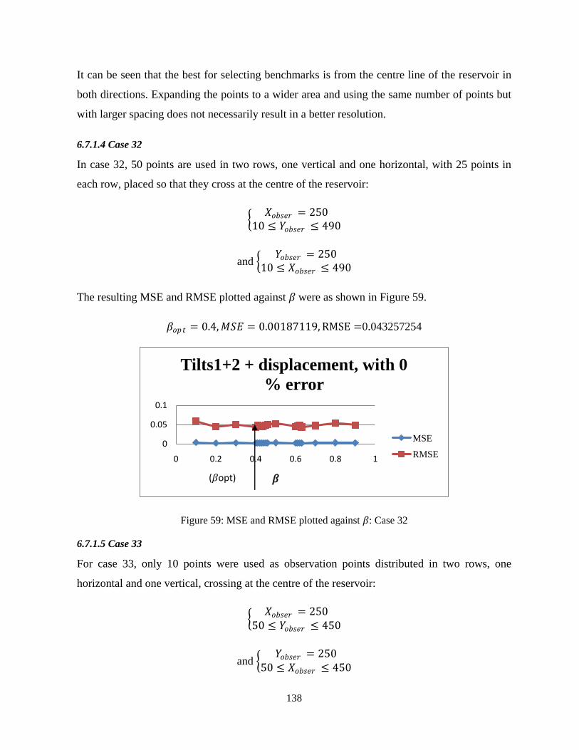
138

It can be seen that the best for selecting benchmarks is from the centre line of the reservoir in

both directions. Expanding the points to a wider area and using the same number of points but

with larger spacing does not necessarily result in a better resolution.

6.7.1.4 Case 32

In case 32, 50 points are used in two rows, one vertical and one horizontal, with 25 points in

each row, placed so that they cross at the centre of the reservoir:


10 ≤ 𝑌𝑜𝑏𝑠𝑒𝑟 ≤ 490


10 ≤ 𝑋𝑜𝑏𝑠𝑒𝑟 ≤ 490


𝛽𝑜𝑝𝑡 = 0.4, 𝑀𝑆𝐸 = 0.00187119, RMSE =0.043257254


6.7.1.5 Case 33

For case 33, only 10 points were used as observation points distributed in two rows, one

horizontal and one vertical, crossing at the centre of the reservoir:


50 ≤ 𝑌𝑜𝑏𝑠𝑒𝑟 ≤ 450


50 ≤ 𝑋𝑜𝑏𝑠𝑒𝑟 ≤ 450

0

0.05

0.1

0 0.2 0.4 0.6 0.8 1

𝛽

Tilts1+2 + displacement, with 0

% error

MSE

RMSE

(𝛽opt)

139

The resulting of MSE and RMSE plotted against 𝛽 were as shown in Figure 60.

𝛽𝑜𝑝𝑡 = 0.3, 𝑀𝑆𝐸 = 0.00224744, RMSE =0.04740717

Figure 60: MSE and RMSE for different values of 𝛽s: Case33.

Table 15 summarises the results of cases 30, 32, and 33, which have the same geometry and

benchmark distribution in 2 rows crossing at the centre of the reservoir, but differ with respect

to the number of points.

Table 15: Comparison of the results of cases 30, 32,and 33.

Case %erro

r

No. of

observati

on points

Distribution of points in two rows 𝜷𝒐𝒑𝒕 𝑴𝑺𝑬𝒎𝒊𝒏 𝑹𝑴𝑺𝑬𝒎𝒊𝒏

30 0% 100 2 rows crossing at the centre of the

reservoir 0.6 0.00179 0.042306


reservoir 0.4 0.001871 0.043257


reservoir 0.3 0.002247 0.047407

As expected, using more points would result in a better resolution.

0

0.02

0.04

0.06

0.08

0.1

0.12

0 0.2 0.4 0.6 0.8 1

𝛽

Tilts1+2 + displacement, with 0 %

error

MSE

RMSE

𝛽(opt)

140

6.8 The effect of the presence of error in the data combined with the omission of

observation points

Thus far, error and the omission of a number of observation points, which limits the input data,

have been examined separately in order to determine the separate effect of each of these factors

on the resolution. In this section the effect of the combination of error and also data limitation

is studied.

6.8.1 Error of 10 %

For the following cases, tilts1+2 from each observation point were used as input data and a

random error of 10 % of the maximum tilt value that was calculated in the observation grid

was added to each input data set for the back-calculation. The results using different

distributions of the benchmarks are also presented in this section.

6.8.1.1 Case 34:

For case 34, 1000 points were distributed in two rows crossing at the centre of the reservoir in

the following range:


−500 ≤ 𝑌𝑜𝑏𝑠𝑒𝑟 ≤ 1000


−500 ≤ 𝑋𝑜𝑏𝑠𝑒𝑟 ≤ 1000


𝛽𝑜𝑝𝑡 = 0.9, 𝑀𝑆𝐸 = 0.10127, RMSE =0.318229

141


6.8.1.2 Case 35

For case 35, 300 points were distributed in two rows crossing at the centre of the reservoir in

the following range:


−500 ≤ 𝑌𝑜𝑏𝑠𝑒𝑟 ≤ 1000

and 𝑌𝑜𝑏𝑠𝑒 𝑟 = 250

−500 ≤ 𝑋𝑜𝑏𝑠𝑒𝑟 ≤ 1000

The results of the inverse solution can be seen in Figure 62.

𝛽𝑜𝑝𝑡 = 0.8, 𝑀𝑆𝐸 = 0.108702, RMSE =0.3297

0

0.2

0.4

0.6

0.8

1

1.2

1.4

0 0.2 0.4 0.6 0.8 1

𝛽

Tilts1+2 + 10 % error

MSE

RMSE

𝛽(opt)

142

Figure 62: MSE and RMSE for different values of 𝛽s: Case 35.

6.8.1.3 Case 36

For case 36, 300 benchmark points are distributed in the area above the reservoir at


0 ≤ 𝑌𝑜𝑏𝑠𝑒𝑟 ≤ 500


0 ≤ 𝑋𝑜𝑏𝑠𝑒𝑟 ≤ 500


𝛽𝑜𝑝𝑡 = 0.2, 𝑀𝑆𝐸 =0.107622, RMSE =0.328058

-1

4

9

14

19

24

29

0 0.2 0.4 0.6 0.8 1

𝛽


MSE

RMSE

𝛽(opt)

143

Figure 63: MSE and RMSE for different values of 𝛽s: Case36.

6.8.1.4 Case 37

Thus far only one distribution geometry has been considered for the observation points. In case

37, the 300 observation points are distributed in six rows: three vertical and three horizontal,

crossing above the centre of the reservoir. Each row has 50 points, one at the centre of each

reservoir element in each row. The plan of the observation points above the reservoir elements

is shown in Figure 64. The spacing between each row of observation points is 10 metres.

Figure 64: Plan of the reservoir with observation points distributed in three vertical and three horizontal

rows crossing above the centre of the reservoir.

The resulting MSE and RMSE plotted against 𝛽 are shown in Figure 65.

𝛽𝑜𝑝𝑡 = 0.1, 𝑀𝑆𝐸 = 0.084998, RMSE =0.291543

0

0.5

1

1.5

2

0 0.2 0.4 0.6 0.8

𝛽


MSE

RMSE

𝛽(opt)

144


6.8.1.5 Case 38

The same distribution used in case 37 was used for case 38 as well, with the exception that the

distance between the rows of observation points was chosen as 100 metres. The observation

data are thus spread out further than in the previous case, as shown in Figure 66.

Figure 66: Plan of the reservoir with the observation points distributed in three vertical and three

horizontal rows above the reservoir.


𝛽𝑜𝑝𝑡 = 0.1, 𝑀𝑆𝐸 = 0.115387, RMSE =0.339687

0

0.5

1

1.5

0 0.2 0.4 0.6 0.8 1

𝛽


MSE

RMSE

𝛽(opt)

145

Figure 67: MSE and RMSE for different values of 𝛽s: Case 38

6.8.1.6 Case 39

For this case, 300 observation points were distributed in 6 vertical rows, with 50 points in each

row. The plan of the observation points is shown in Figure 68.

Figure 68: Plan of the reservoir with observation points distributed in six vertical rows above the centre

of the reservoir.

The results can be seen in Figure 69.

𝛽𝑜𝑝𝑡 = 0.2, 𝑀𝑆𝐸 = 0.04971, RMSE =0.222957

-5

0

5

10

15

20

0 0.1 0.2 0.3 0.4 0.5 0.6 0.7

𝛽

Tilt1+2 + 10 % error

MSE

RMSE

𝛽(opt)

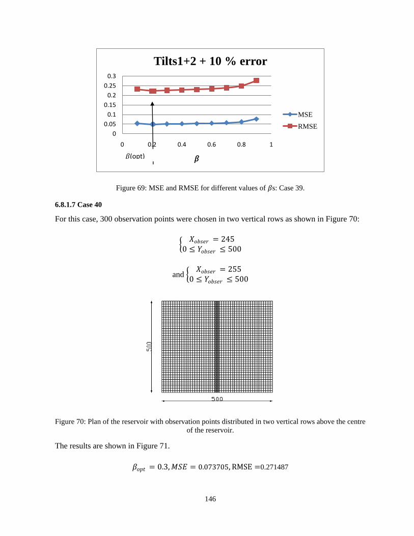
146


6.8.1.7 Case 40

For this case, 300 observation points were chosen in two vertical rows as shown in Figure 70:


0 ≤ 𝑌𝑜𝑏𝑠𝑒𝑟 ≤ 500

and 𝑋𝑜𝑏𝑠𝑒𝑟 = 255

0 ≤ 𝑌𝑜𝑏𝑠𝑒𝑟 ≤ 500

Figure 70: Plan of the reservoir with observation points distributed in two vertical rows above the centre

of the reservoir.

The results are shown in Figure 71.

𝛽𝑜𝑝𝑡 = 0.3, 𝑀𝑆𝐸 = 0.073705, RMSE =0.271487

0

0.05

0.1

0.15

0.2

0.25

0.3

0 0.2 0.4 0.6 0.8 1

𝛽


MSE

RMSE

𝛽(opt)

147


6.8.1.8 Case 41:

In case, 100 points were used as observation points in two rows, with 50 horizontal and 50

vertical points. The results can be seen in Figure 72.

𝛽𝑜𝑝𝑡 = 0.2, 𝑀𝑆𝐸 = 0.140679, RMSE =0.375072


As a basis of comparison, the results of the cases considered in this section, with 10% error, are

summarised in Table 16.

0

0.5

1

1.5

2

0 0.2 0.4 0.6 0.8

𝛽


MSE

RMSE

0

0.2

0.4

0.6

0.8

0 0.2 0.4 0.6 0.8

𝛽

Tilts1+2, with 10 % of the points

MSE

RMSE

𝛽(opt)

𝛽(opt)

148

Table 16: Summary of results with respect to the effect of the number and distribution of observation

points along with the error present in the observation data.

Tilt1+tilt2+10% error

Case

No. Of

observation

points

bench mark distribution 𝜷𝒐𝒑𝒕 𝑴𝑺𝑬𝒎𝒊𝒏 𝑹𝑴𝑺𝑬𝒎𝒊𝒏

34 1000 2 rows, 1 vertical, 1 horizontal-500,1000 0.9 0.10127 0.318229

35 300 2 rows, 1 vertical, 1 horizontal-500,1000 0.8 0.108702 0.3297

36 300 2 rows, 1 vertical, 1 horizontal - 0,500 0.2 0.107622 0.328058

37 300 6 rows, 3 vertical, 3 horizontal, 10 m

spacing between rows - 0,500 0.1 0.084998 0.291543

38 300 6 rows, 3 vertical, 3 horizontal, 100 m

spacing between rows -,0,500 0.1 0.115387 0.339687

39 300 6 vertical rows, 10 m spacing between rows

- 0,500 0.2 0.04971 0.222957

40 300 2 vertical rows, 10 m spacing between rows

-,0,500 0.3 0.073705 0.271487

41 100 2 rows, 1 vertical, 1 horizontal - 0,500 0.2 0.140679 0.375072

As can be seen, using 300 points, in case 39, results in a much better resolution than does using

1000 points in case 34. The importance of the geometry of the benchmarks chosen can be seen

by comparing the results presented in Table 16.

If cases 35 and 36 are compared, the MSE in case 35 is a bit higher than in case 36 but still

very close. However, volume change distribution graphs (Appendix V includes the complete

graphs) for the two cases show totally different results. The graphs for Case 35 are better

approximation of the initial volume (Figure 73).

The MSE or RMSE alone are not sufficient factors for evaluating the solutions. Another shape

factor thus must be developed in order to describe the differences in the graphs of the inverse

solutions.

149

Figure 73: It can be seen although MSE being very close, the distribution is totally different.

6.8.2 Case of 5% error

6.8.2.1 Case 42

As can be seen from Table 16, it can be concluded that the best distribution of observation

points is vertical placement in one direction, which in this study was the case that with 6

vertical rows of benchmarks, each row being placed above the centre of the reservoir elements,

with distances equal to the sizes of the reservoir elements. This distribution was therefore

considered for case 42 as well, and 300 observation points with the same reservoir geometry

and initial volume changes were assumed. The error considered was 5 % of the maximum

value of the calculated tilt, and this error was added to tilts. This data was then used as input

for the back-calculations. The results are as shown in Figure 74.

-7

-5

-3

-1

1

0 20 40 60

Volu

me

chan

ge

The No of reservoit element in each row

300 observation points

(-500,1000), 10 % error, (case 35)

Row1-initial

Row1-calculated

Row2-initial

Row2-calculated

Row3-initial

-8

-6

-4

-2

0

2

0 20 40 60

Volu

me

cha

ng

e

No of reservoit element in each row

300 observation points (0,500),

10 % error, case 36

Row1-initial

Row1-calculated

Row2-initial

Row2-calculated

Row3-initial

Row3-calculated

Row4-initial

150

𝛽𝑜𝑝𝑡 = 0.1, 𝑀𝑆𝐸 = 0.013457, RMSE =0.116004


6.8.3 Case of 3 % error

6.8.3.1 Case 43

All input and geometry are identical to those for case 42. Only a 3 % random error is added to

the tilts at each observation point. The results of the inverse solution can be seen in Figure 75.

𝛽𝑜𝑝𝑡 = 0.2, 𝑀𝑆𝐸 = 0.006455, RMSE =0.080343

0

0.05

0.1

0.15

0.2

0.25

0.3

0 0.2 0.4 0.6 0.8 1

𝛽


MSE

RMSE

𝛽(opt)

151


Table 17 provides a summary and comparison of the results of investigating the sensitivity of

the calculation to error with a limited number of observation points. The number of observation

points chosen was 300, which is only 12 % of the unknowns to be solved for. The results are

listed for different percentage of error.

Table 17: Comparison of results: the effect of error for the best benchmark distribution

Case Error Number of

observation points Benchmark distribution 𝜷𝒐𝒑𝒕 𝑴𝑺𝑬𝒎𝒊𝒏 𝑹𝑴𝑺𝑬𝒎𝒊𝒏

39 10% 300 6 vertical rows, distance between

rows 10 m- 0,500 0.2 0.04971 0.222957


rows 10 m- 0,500 0.1 0.013457 0.116004


rows 10 m- 0,500 0.2 0.006455 0.080343

From Table 17 and a comparison of the graphs of the cases provided in the Appendix V, it can

be seen that in the case with an error of 10 % for 300 benchmarks (12% of the number of

unknown values), the results of the calculations vary significantly relative to the actual

assigned values. In the case with an error of 5 %, however, the graphs show better calculated

values compared to those for the 10 % error. With respect to the 3 % error, the results are quite

acceptable, and the graphs show a suitable distribution of the changes in volume.

0

0.05

0.1

0.15

0.2

0 0.1 0.2 0.3 0.4 0.5 0.6

𝛽


MSE

RMSE

𝛽(opt)

152

6.8.4 20 observation points with 1 % error: case 44

In reality, using 300 points as observation points, which means using 300 tilt meters to observe

the deformations using tilts, is not practical. Therefore, in this section, 20 observation points

were chosen, placed in 4 rows of 5 with a spacing of 20 m and located in the mid-section of the

reservoir, as shown in Figure 76.

Figure 76: Observation grid of 20 points.



and 78.

153


-3

-2

-1

0

1

2

0 20 40 60

Va

lue

s

X-direction

Line @ Y = 1

Assumed Calculated

-3

-2

-1

0

1

2

0 20 40 60

Va

lue

s

X-direction

Line @ Y = 2

Assumed Calculated

-3

-2

-1

0

1

2

0 20 40 60

Va

lue

s

X-direction

Line @ Y = 3

Assumed Calculated

-3

-2

-1

0

1

2

0 20 40 60

Va

lue

s

X-direction

Line @ Y = 4

Assumed Calculated

-3

-2

-1

0

1

2

0 20 40 60

Va

lue

s

X-direction

Line @ Y = 5

Assumed Calculated

-3

-2

-1

0

1

2

0 20 40 60

Va

lue

s

X-direction

Line @ Y = 6

Assumed Calculated

154


-2

-1.5

-1

-0.5

0

0.5

1

0 20 40 60

Val

ue

s

X-direction

Line @ Y = 25

Assumed Calculated

-2

-1.5

-1

-0.5

0

0.5

1

0 20 40 60

Val

ue

s

X-direction

Line @ Y = 26

Assumed Calculated

-2.5

-2

-1.5

-1

-0.5

0

0.5

1

0 20 40 60

Val

ue

s

X-direction

Line @ Y = 27

Assumed Calculated

-2.5

-2

-1.5

-1

-0.5

0

0.5

1

0 20 40 60V

alu

es

X-direction

Line @ Y = 28

Assumed Calculated

-2.5

-2

-1.5

-1

-0.5

0

0.5

0 20 40 60

Val

ue

s

X-direction

Line @ Y = 29

Assumed Calculated

-2.5

-2

-1.5

-1

-0.5

0

0.5

0 20 40 60

Val

ue

s

X-direction

Line @ Y = 30

Assumed Calculated

155

It could be seen that using 20 points with only a 1 % error would not result in an acceptable

remodelling. Therefore, since errors are always present in data, the number of observation

points affects the results of the reconstructed values more significantly.

156

7.0 Conclusions

A numerical model for calculating surface deformations due to volumetric changes in a

reservoir has been developed as the first part of this study. However, the main focus is on the

solution of the inverse case, for which a computer code has been developed in C++ (1080

lines).

The computer codes written for the direct and the inverse cases have been verified. The direct

case was verified using a checklist of numerical calculations as presented by Okada (1985).

With respect to the inverse case, the results from the inversion of the direct solutions with 0 %

error are used for the reconstruction of volume changes.

The calculations for these models are all based on generic subsurface changes in volume; the

results can thus be applied to a variety of applications and types of reservoirs (e.g.,

hydrocarbon, underground water, geysers, waste reinjection projects, steam injection). The

following summary and conclusions from the cases investigated are valid for all types of

reservoirs:

The RMSE of back-calculated changes in volume compared to the initial assumed

values plotted for different reservoir elements shows fluctuations at some reservoir

points and not at other points. The RMSE is much higher for the corner rows than for

the middle rows. Thus, the inverse solution is poor for corner elements.

For the case of the parameter 𝛽=0 (no regularization), the greater the depth of the

reservoir, the more ill-conditioned the problem becomes Thus, for very shallow depths,

the problem tends to be well-posed.

Tilt measurements are more effective than vertical displacement measurements for

inverting reservoir volumetric changes in the reservoir that occur at different depths.

For the case of tilt measurements with no errors, the computed RMSE value is

smaller than the computed value for vertical displacements (by about 12 % in

the case studied).

The presence of small errors in the measured displacement data (<0.55 % of the

maximum surface displacement) generates significant deviations in the solution

from the actual value. However, for tilt measurements with errors of up to 20 %

157

of the maximum tilt value, a reasonable reconstruction of the original volume

changes is possible. It should be noted that an error of 10 % is considered

reasonable for tilt measurements. Therefore, it is recommended that tilt

measurements rather than vertical displacements be used as input data.

The required area of observation can be reduced if tilt measurements are used,

which would make the setup process for collecting experimental data more

convenient.

The predictions of changes in volume when tilt1(dz/dx) is used as input versus those

generated when tilt2(dz/dy) is used as input for an identical case are almost identical.

The best deformation data to be used as input were found to be Tilt1+Tilt2 together.

Based on sensitivity analysis, when used as input data, displacement data were found to

be much more sensitive to error than tilts are.

For an error of zero, when tilts are used, very good resolution is obtainable using only

0.4 % of the number of unknowns as the number of benchmarks. That is, using only 10

observation points in the case of solving for a reservoir with 2500 elements (2500

unknowns to be solved) resulted in an acceptable reconstruction.

Errors in the input data are more influential than the number of observation points for

inverse solutions.

The distribution of benchmark points significantly affects the results. The best

distribution of benchmarks was found to be a parallel set of rows. The optimal spacing

resulting in the solution with the highest resolution was found to be equal to the sizes of

the elements in the reservoir.

In some cases, although the RMSE of the results are very similar, the plots of the

changes in volume change are different. Thus, it is of great importance to analyze the

distribution of volume changes in order to provide an understanding of the behaviour of

the reservoir during reinjection or production projects.

158

8. Future work and recommendations

The consolidation of soils and the development of deformations usually takes time.

How long is required for the entire deformation to be transferred to the surface depends

on the overburden material, the history of the formation, and other factors. Thus the

induced subsidence or upheaval observed on the surface and recorded might not

represent the entire extent of the deformation. Therefore, using this data as input for the

inverse problem can result in a misleading reconstruction and modeling of the inverse

case. For future work, it is suggested that the time factor be considered and investigated

for use in the inverse modeling.

For the numerical modeling in this and most studies, one of the basic assumptions is

that the media is isotropic and homogeneous. In reality, this is not the case. For future

research, it is recommended that the effect of layering on models and the inverse ill-

posed solution be considered and examined.

Subsurface volume changes can be used to predict earthquakes. Surface deformation

data can be recorded for areas above active faults and in zones that have the potential

for earthquakes and can then be used to monitor changes in volume that occur in active

zones. These changes in volume could possibly be converted to factors that could be

helpful in predicting earthquakes.

The inverse problem in the case of the presence of more than one source of subsurface

deformation is also recommended as an area for further study.

159

References

Allis, R. G. (2000). Review of Subsidence at Wairakei Field, NewZealand. Geothermics ,

455-478.

Amyx, J. W., Bass, D. M., & Whiting, R. L. (1960). Petroleum Reservoir Engineering

Physical Properties.

Bilak, R. A. (1989). Analysis of Surface Deformation Above Hydrocarbon Producing

Reservoirs. Waterloo.

Biot, M. A. (1956). Appl. phys, 27,240 .

Bruno, M. S., & Bovberg, C. A. (1992). Reservoir Compaction and Surface Subsidence

Above the Lost Hills Field, California, The 33th U.S. Symposium on Rock Mechanics, 92-

0263.

Bruno, M. S., & Co, C. O. (1990). Subsidence-Induced Well Failure. SPE , 383-390.

Calhoun, J. (1917). Fundamentals of Reservoir Engineering. Norman, University of

Oklahoma Press c1960 .

Carnec, C., & Fabriol, H. (1999). Monitoring and Modeling Land Subsidence at the Cerro

Prieto Geothermal Field, Baja California, Mexico, Using SAR Interferometry. Geophysical

Research letters, VOL. 26, NO. 9, Pages 1211-1214, MAY 1, 1999.

Chan, A. W., & Zoback, M. D. (2007). The Role of Hydrocarbon Production on Land

Subsidence and Fault Reactivation in the Louisiana Coastal Zone. Journal of Coastal

Research , 771–786.

Chen, C.-T., Hu, J.-C., Lu, C.-Y., Lee, J.-C., & Chan, Y.-C. (2007). Thirty-Year Land

Elevation Change from Subsidence to Uplift Following the Termination of Groundwater

Pumping and its Geological Implications in the Metropolitan Taipei Basin, Northern

Taiwan. Engineering Geology , 30-47.

Chin, L., Boade, R. R., Prevost, J. H., & Landa, G. H. (1993). Numerical Simulation of

Shear-Induced Compaction in the Ekofisk Reservoir. Int. J. Rock Mech. Min. Sci. &

Geomech , 1193-1200.

Cosse, R. (1993). Oil and Gas Field Development Techniques: Basics of Reservoir

Engineering. Paris.

Das, B. M. (Sixth Edition,2006). Principles of Geotechnical Engineering. California.

160

Du, J., & Olson, J. E. (2001). A Poroelastic Reservoir Model for Predicting Subsidence and

Mapping Subsurface Pressure Fronts. Journal of Petroleum Science and Engineering ,

181–197.

Dusseault, M. B., & Rothenburg, L. (2002). Analysis of Deformation Measurements for

Reservoir Management. Oil & Gas Science and Technology , 539-554.

Dusseault, M. B., Bilak, R. A., & Rothenburg, L. (1993). Inversion of Surface

Displacements to Monitor In Situ Processes. lnL J. Rock Mech. Min. Sci, & Geomech ,

1219-1222.

Engl, H. W., & Groetsch, C. W. (1987). Inverse and Ill-posed Problems. London:

Academic Press, INC.

Ferretti, A., Novali, F., & Vasco, D. W. (2008). Reservoir Monitoring and Characterization

Using Satellite Geodetic Data: Interferometric Synthetic Aperture Radar Observations from

the Krechba field, Algeria. GEOPHYSICS,VOL. 73 , 113–122.

Galloway, D. L., Hudnut, K. W., Ingebritsen, S. E., Phillips, S. P., Peltzer, G., Rogez, F., et

al. (1998). Detection of Aquifer System Compaction and Land Subsidence Using

Interferometric Synthetic Aperture Radar, Antelope Valley, Mojave Desert, California.

Water Resources Research , 2573-2585.

Gambolati, G. (1975). Numerical Models in Land Subsidence Control. Cmputer Methods

in Applied Mechanics and Engineering, 227-237.

Geertsma, J. (1957). A Remark on the Analogy Between Thermoelasticityand the Elasticity

of Saturated Porous Media. Journal of the Mechanics and Physics of Solids , 13-16.

Geertsma, J. (1973). Land Subsidence Above Compacting Oil and Gas Reservoirs.

JOURNAL OF PETROLEUM TECHNOLOGY , 734-744.

Geertsma, J. (1957). The Effect of Fluid Pressure Decline on Volumetric Changes of

Porous Rocks. Trans. AIME, 210, 331–340.

Glowacka, E., Gonzalez, J., & Fabriol, H. (1999). Recent Vertical Deformation in Mexicali

Valley and its Relationship with Tectonics, Seismicity, and the Exploitation of the Cerro

Prieto Geothermal Field, Mexico. Pure appl. geophys , 591-614.

Gurevich, A. E., & Chilingarian, G. V. (1993). Subsidence Over Producing Oil and Gas

Fields, and Gas Leakage to the Surface. Journal of Petroleum Science and Engineering ,

239-250.

161

Hermansen, H., Landa, G. H., Sylte, J. E., & Thomas, L. K. (2000). Experiences After 10

Years of Waterflooding the Ekofisk Field,Norway. Journal of Petroleum Science and

Engineering , 11-18.

Hu, R. L., Yue, Z. Q., Wang, L. C., & Wang, S. J. (2004). Review on Current Status and

Challenging Issues of Land Subsidence in China. Engineering Geology , 65– 77.

J. Carlos Santamaria, D. F. (2005). Discrete Signals and Inverse Problems.

Kroon, I. C., Nguyen, B. L., Fokker, P. A., Muntendam-Bos, A. G., & Lange, G. d. (2008).

Disentangling Shallow and Deep Processes Causing Surface Movement. International

Association for Mathematical Geosciences .

Nagel, N. B. (2001). Compaction and Subsidence Issues Within the Petroleum Industry:

From Wilmington to Ekofisk and Beyond. Phys. Chem. Earth , Vol. 26, No. 1-2, pp. 3-14.

Okada, Y. (1985). Surface Deformation Due to Shear and Tensile Faults in a Half-Space.

Bulletin of the Seismological Society of America , Vol. 75, No. 4, pp. 1135-1154.

Press, W. H., Teukolsky, S. A., Vetterling, W. T., & Flannery, B. P. (1988). Numerical

Recipes in C. Press Syndicate of university of Cambridge.

Rothenburg, L., Dusseault, M. B., Bilak, R. A., & Bruno, M. S. (1994). Waste Disposal

Monitoring Using the Surface Displacement Field. Society of Petroleum Engineers , 29-31.

Segall, P. (1985). Stress and Subsidence Resulting from Subsurface Fluid Withdrawal in

the Epicentral Region of the 1983 Coalinga Earthquake. J. Geophys. Res., 90, 6801– 6816.

Tikhonov, A. N., & Arsenin, V. Y. (1977). Solutions of Ill-posed Problems.

Vardoulakis, I., Vairaktaris, E., & Papamicho, E. (2004). Subsidence Diffusion–

Convection: I. The Direct Problem. Comput. Methods Appl. Mech. Engrg , 2745–2760.

Vasco, D. W. (2004). Estimation of Flow Properties Using Surface Deformation and Head

Data: A Trajectory-Based Approach. Water Resources Research, VOL. 40.

Vasco, D. W., Wicks, C. J., Karasaki, K., & Marques, O. (2002). Geodetic Imaging:

Reservoir Monitoring Using Satellite Interferometry. Geophys. J. Int , 555–571.

162

Appendix

Appendix I: Calculating the L matrix

Calculating the L matrix

As mentioned in the previous section the problem of solving the ill-posed equation of

calculating reservoir volume changes based on surface deformation data came to solving the

following equation:


K matrix was described in detail in section4.6. 𝛽 also is a number chosen between zero and

one. ∆𝑣 the unknown matrix and U is the known matrix from surface deformation data as

mentioned in section4.6. In this section calculating the L matrix is of intention. The reservoir

can be assumed to be very thin, thus we can deal with the problem as two dimensional. Thus

the surface deformation can be written as:

𝑑𝑍

𝑑𝑠=

𝜕2𝐸𝑣

𝜕𝑥2+

𝜕2𝐸𝑣

𝜕𝑦2

If looking at a one dimensional case, thus the partial derivative would be as follows:

𝜕𝑢

𝜕𝑥=

𝑢𝑖+1 − 𝑢𝑖 − 𝑢𝑖 − 𝑢𝑖−1

∆𝑥=

𝑢𝑖+1 + 𝑢𝑖−1 − 2𝑢𝑖

∆𝑥

In our case, 𝑢𝑖 represents the volume change in the 𝑖𝑡𝑕 reservoir element.

The second derivative with respect to ∆𝑥 would thus be:

𝜕2𝑢

𝜕𝑥2=

𝑢𝑖+1 + 𝑢𝑖−1 − 2𝑢𝑖

∆𝑥∗

1

∆𝑥=

𝑢𝑖+1 + 𝑢𝑖−1 − 2𝑢𝑖

∆𝑥2

As for our case which is a two dimensional problem we would have:

𝜕2𝑢

𝜕𝑥2+

𝜕2𝑢

𝜕𝑦2=

𝑢𝑖+1,𝑗 + 𝑢𝑖−1,𝑗 − 2𝑢𝑖 ,𝑗

∆𝑥2+

𝑢𝑗+1,𝑖 + 𝑢𝑗−1,𝑖 − 2𝑢𝑗 ,𝑖

∆𝑦2= 0

We are looking at a reservoir grid, where ∆𝑥 𝑎𝑛𝑑 ∆𝑦 is the grid spacing is two directions. A

representative part of reservoir grid is shown as follows:

163

As for a specific case we consider∆𝑥 = ∆𝑦 = 𝑕.

For the mid reservoir elements the second derivative can be easily explained using the above

equation. For the elements on the corner of the reservoir, we assume that we do have a row of

data points outside the grid and their volume changes are assumed to be equal to that of the

inside row. See the following example:

A 4*4 reservoir element (N=16) is used to show the procedures of constructing a Laplacian

matrix to solve for the inverse ill-posed problem:

13 14 15 16

1 2 3 4

5 6 7 8

9 10 11 12

0

h

h

i+1

i

i-1

j-1 j j+1

X

Y

164

Each point represents a reservoir element’s volume change. The dotted rows all around the

reservoir grid is the imaginary row of elements with the same volume changes as the one right

across and inside. For point 0 for instance, 𝑉10 = 𝑉12 .

For 1𝑠𝑡 and 2𝑛𝑑 rows the elements for the Laplacian matrix are calculated as follows:

𝐹𝑜𝑟 𝑝𝑜𝑖𝑛𝑡 1 = −𝑣15 + 𝑣15 + 𝑣12 + 𝑣12 − 4 ∗ 𝑣11

𝑕2= −

2𝑣15 + 2𝑣12 − 4𝑣11

𝑕2

𝐹𝑜𝑟 𝑝𝑜𝑖𝑛𝑡 2 = −𝑣21 + 𝑣23 + 𝑣26 + 𝑣26 − 4 ∗ 𝑣22

𝑕2= −

𝑣21 + 𝑣23 + 2𝑣26 − 4𝑣22

𝑕2

𝐹𝑜𝑟 𝑝𝑜𝑖𝑛𝑡 3 = −𝑣32 + 𝑣34 + 𝑣37 + 𝑣37 − 4 ∗ 𝑣33

𝑕2= −

𝑣32 + 𝑣34 + 2𝑣37 − 4𝑣33

𝑕2

𝐹𝑜𝑟 𝑝𝑜𝑖𝑛𝑡 4 = −2𝑣43 + 2𝑣48 − 4𝑣44

𝑕2

𝐹𝑜𝑟 𝑝𝑜𝑖𝑛𝑡 5 = −𝑣51 + 𝑣59 + 2𝑣56 − 4 ∗ 𝑣55

𝑕2

𝐹𝑜𝑟 𝑝𝑜𝑖𝑛𝑡 6 = −𝑣65 + 𝑣67 + 𝑣610 + 𝑣62 − 4 ∗ 𝑣66

𝑕2

....

The L matrix formed for a 4*4 reservoir with 16 elements is as follows using the

abovementioned procedure. The elements with no numbers have all zero values.

165

[𝐿]16∗16 =

1 2 3 4 5 6 7 8 9 10 11 12 13 14 15 16

1 4

𝑕2 −2

𝑕2 −2

𝑕2

2 −1

𝑕2 4

𝑕2 −1

𝑕2 −2

𝑕2

3 −1

𝑕2 4

𝑕2 −1

𝑕2 −2

𝑕2

4 −2

𝑕2 4

𝑕2 −2

𝑕2

5 −1

𝑕2 4

𝑕2 −2

𝑕2 −1

𝑕2

6 −1

𝑕2 −1

𝑕2 4

𝑕2 −1

𝑕2 −1

𝑕2

7 −1

𝑕2 −1

𝑕2 4

𝑕2 −1

𝑕2 −1

𝑕2

8 −1

𝑕2 −2

𝑕2 4

𝑕2 −1

𝑕2

9 −1

𝑕2 4

𝑕2 −2

𝑕2 −1

𝑕2

10 −1

𝑕2 −1

𝑕2 4

𝑕2 −1

𝑕2 −1

𝑕2

11 −1

𝑕2 −1

𝑕2 4

𝑕2 −1

𝑕2 −1

𝑕2

12 −1

𝑕2 −2

𝑕2 4

𝑕2 −1

𝑕2

13 −2

𝑕2 4

𝑕2 −2

𝑕2

14 −2

𝑕2 −1

𝑕2 4

𝑕2 −1

𝑕2

15 −2

𝑕2 −1

𝑕2 4

𝑕2 −1

𝑕2

16 −2

𝑕2 −2

𝑕2 4

𝑕2

166

Appendix II: Graphs: limiting observation area

Case4, using tilt2, 𝛽=0.0000003, RMSE=0.02436, -500<X,Y<1000

-0.4

-0.3

-0.2

-0.1

0

0 20 40 60

Val

ue

s

X-direction

Line @ Y = 1

Assumed Calculated

-0.4

-0.3

-0.2

-0.1

0

0 20 40 60

Val

ue

s

X-direction

Line @ Y = 2

Assumed Calculated

-0.4

-0.3

-0.2

-0.1

0

0 20 40 60

Val

ue

s

X-direction

Line @ Y = 3

Assumed Calculated

-0.5

-0.4

-0.3

-0.2

-0.1

0

0 20 40 60

Val

ue

s

X-direction

Line @ Y = 4

Assumed Calculated

-0.5

-0.4

-0.3

-0.2

-0.1

0

0 20 40 60

Val

ue

s

X-direction

Line @ Y = 5

Assumed Calculated

-0.5

-0.4

-0.3

-0.2

-0.1

0

0 20 40 60

Val

ue

s

X-direction

Line @ Y = 6

Assumed Calculated

167

-1.2

-1

-0.8

-0.6

-0.4

-0.2

0

0 20 40 60

Val

ue

s

X-direction

Line @ Y = 25

Assumed Calculated

-1.2

-1

-0.8

-0.6

-0.4

-0.2

0

0 20 40 60

Val

ue

s

X-direction

Line @ Y = 26

Assumed Calculated

-1.2

-1

-0.8

-0.6

-0.4

-0.2

0

0 20 40 60

Val

ue

s

X-direction

Line @ Y = 27

Assumed Calculated

-1.2

-1

-0.8

-0.6

-0.4

-0.2

0

0 20 40 60

Val

ue

s

X-direction

Line @ Y = 28

Assumed Calculated

-1.2

-1

-0.8

-0.6

-0.4

-0.2

0

0 20 40 60

Val

ue

s

X-direction

Line @ Y = 29

Assumed Calculated

-1.2

-1

-0.8

-0.6

-0.4

-0.2

0

0 20 40 60

Val

ue

s

X-direction

Line @ Y = 30

Assumed Calculated

168

Case7: Using tilt2 as input, 0% error,−5 ≤ 𝑋𝑜𝑏𝑠𝑒𝑟 , 𝑌𝑜𝑏𝑠𝑒𝑟 ≤ 505

-0.5

-0.4

-0.3

-0.2

-0.1

0

0 20 40 60

Val

ue

s

X-direction

Line @ Y = 1

Assumed Calculated

-0.5

-0.4

-0.3

-0.2

-0.1

0

0 20 40 60

Val

ue

s

X-direction

Line @ Y = 2

Assumed Calculated

-0.5

-0.4

-0.3

-0.2

-0.1

0

0 20 40 60

Val

ue

s

X-direction

Line @ Y = 3

Assumed Calculated

-0.5

-0.4

-0.3

-0.2

-0.1

0

0 20 40 60V

alu

es

X-direction

Line @ Y = 4

Assumed Calculated

-0.5

-0.4

-0.3

-0.2

-0.1

0

0 20 40 60

Val

ue

s

X-direction

Line @ Y = 5

Assumed Calculated

-0.5

-0.4

-0.3

-0.2

-0.1

0

0 20 40 60

Val

ue

s

X-direction

Line @ Y = 6

Assumed Calculated

169

-1.2

-1

-0.8

-0.6

-0.4

-0.2

0

0 20 40 60

Val

ue

s

X-direction

Line @ Y = 25

Assumed Calculated

-1.2

-1

-0.8

-0.6

-0.4

-0.2

0

0 20 40 60

Val

ue

s

X-direction

Line @ Y = 26

Assumed Calculated

-1.2

-1

-0.8

-0.6

-0.4

-0.2

0

0 20 40 60

Val

ue

s

X-direction

Line @ Y = 27

Assumed Calculated

-1.2

-1

-0.8

-0.6

-0.4

-0.2

0

0 20 40 60V

alu

es

X-direction

Line @ Y = 28

Assumed Calculated

-1.2

-1

-0.8

-0.6

-0.4

-0.2

0

0 20 40 60

Val

ue

s

X-direction

Line @ Y = 29

Assumed Calculated

-1.2

-1

-0.8

-0.6

-0.4

-0.2

0

0 20 40 60

Val

ue

s

X-direction

Line @ Y = 30

Assumed Calculated

170

Appendix III: Graphs; error in input data

Case9:Tilt1+2 with 3% error, RMSE=0.26796

-0.6

-0.4

-0.2

0

0.2

0 20 40 60

Val

ue

s

X-direction

Line @ Y = 1

Assumed Calculated

-0.6

-0.4

-0.2

0

0.2

0 20 40 60

Val

ue

s

X-direction

Line @ Y = 2

Assumed Calculated

-0.6

-0.4

-0.2

0

0.2

0 20 40 60

Val

ue

s

X-direction

Line @ Y = 3

Assumed Calculated

-0.6

-0.4

-0.2

0

0.2

0 20 40 60

Val

ue

s

X-direction

Line @ Y = 4

Assumed Calculated

-0.6

-0.4

-0.2

0

0.2

0 20 40 60

Val

ue

s

X-direction

Line @ Y = 5

Assumed Calculated

-0.8

-0.6

-0.4

-0.2

0

0 20 40 60

Val

ue

s

X-direction

Line @ Y = 6

Assumed Calculated

171

-1.2

-1

-0.8

-0.6

-0.4

-0.2

0

0 20 40 60

Val

ue

s

X-direction

Line @ Y = 25

Assumed Calculated

-1.2

-1

-0.8

-0.6

-0.4

-0.2

0

0 20 40 60

Val

ue

s

X-direction

Line @ Y = 26

Assumed Calculated

-1.2

-1

-0.8

-0.6

-0.4

-0.2

0

0 20 40 60

Val

ue

s

X-direction

Line @ Y = 27

Assumed Calculated

-1.2

-1

-0.8

-0.6

-0.4

-0.2

0

0 20 40 60

Val

ue

s

X-direction

Line @ Y = 28

Assumed Calculated

-1.2

-1

-0.8

-0.6

-0.4

-0.2

0

0 20 40 60

Val

ue

s

X-direction

Line @ Y = 29

Assumed Calculated

-1.2

-1

-0.8

-0.6

-0.4

-0.2

0

0 20 40 60

Val

ue

s

X-direction

Line @ Y = 30

Assumed Calculated

172

Case10:

Tilt 1&2 with maximum error of 6% RMSE= 0.0779796

-0.6

-0.4

-0.2

0

0.2

0 20 40 60

Val

ue

s

X-direction

Line @ Y = 1

Assumed Calculated

-0.8

-0.6

-0.4

-0.2

0

0.2

0 20 40 60

Val

ue

s

X-direction

Line @ Y = 2

Assumed Calculated

-0.8

-0.6

-0.4

-0.2

0

0.2

0 20 40 60

Val

ue

s

X-direction

Line @ Y = 3

Assumed Calculated

-0.8

-0.6

-0.4

-0.2

0

0.2

0 20 40 60

Val

ue

s

X-direction

Line @ Y = 4

Assumed Calculated

-0.8

-0.6

-0.4

-0.2

0

0.2

0 20 40 60

Val

ue

s

X-direction

Line @ Y = 5

Assumed Calculated

-0.8

-0.6

-0.4

-0.2

0

0.2

0 20 40 60

Val

ue

s

X-direction

Line @ Y = 6

Assumed Calculated

173

-1.2

-1

-0.8

-0.6

-0.4

-0.2

0

0 20 40 60

Val

ue

s

X-direction

Line @ Y = 25

Assumed Calculated

-1.2

-1

-0.8

-0.6

-0.4

-0.2

0

0 20 40 60

Val

ue

s

X-direction

Line @ Y = 26

Assumed Calculated

-1.2

-1

-0.8

-0.6

-0.4

-0.2

0

0 20 40 60

Val

ue

s

X-direction

Line @ Y = 27

Assumed Calculated

-1.2

-1

-0.8

-0.6

-0.4

-0.2

0

0 20 40 60

Val

ue

s

X-direction

Line @ Y = 28

Assumed Calculated

-1.2

-1

-0.8

-0.6

-0.4

-0.2

0

0 20 40 60

Val

ue

s

X-direction

Line @ Y = 29

Assumed Calculated

-1.2

-1

-0.8

-0.6

-0.4

-0.2

0

0 20 40 60

Val

ue

s

X-direction

Line @ Y = 30

Assumed Calculated

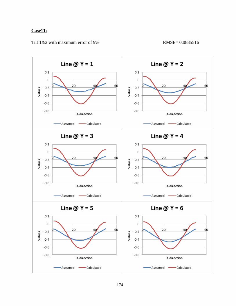
174

Case11:

Tilt 1&2 with maximum error of 9% RMSE= 0.0885516

-0.8

-0.6

-0.4

-0.2

0

0.2

0 20 40 60

Val

ue

s

X-direction

Line @ Y = 1

Assumed Calculated

-0.8

-0.6

-0.4

-0.2

0

0.2

0 20 40 60

Val

ue

s

X-direction

Line @ Y = 2

Assumed Calculated

-0.8

-0.6

-0.4

-0.2

0

0.2

0 20 40 60

Val

ue

s

X-direction

Line @ Y = 3

Assumed Calculated

-0.8

-0.6

-0.4

-0.2

0

0.2

0 20 40 60

Val

ue

s

X-direction

Line @ Y = 4

Assumed Calculated

-0.8

-0.6

-0.4

-0.2

0

0.2

0 20 40 60

Val

ue

s

X-direction

Line @ Y = 5

Assumed Calculated

-0.8

-0.6

-0.4

-0.2

0

0.2

0 20 40 60

Val

ue

s

X-direction

Line @ Y = 6

Assumed Calculated

175

-1.2

-1

-0.8

-0.6

-0.4

-0.2

0

0 20 40 60

Val

ue

s

X-direction

Line @ Y = 25

Assumed Calculated

-1.2

-1

-0.8

-0.6

-0.4

-0.2

0

0 20 40 60

Val

ue

s

X-direction

Line @ Y = 26

Assumed Calculated

-1.2

-1

-0.8

-0.6

-0.4

-0.2

0

0 20 40 60

Val

ue

s

X-direction

Line @ Y = 27

Assumed Calculated

-1.2

-1

-0.8

-0.6

-0.4

-0.2

0

0 20 40 60

Val

ue

s

X-direction

Line @ Y = 28

Assumed Calculated

-1.2

-1

-0.8

-0.6

-0.4

-0.2

0

0 20 40 60

Val

ue

s

X-direction

Line @ Y = 29

Assumed Calculated

-1.2

-1

-0.8

-0.6

-0.4

-0.2

0

0 20 40 60

Val

ue

s

X-direction

Line @ Y = 30

Assumed Calculated

176

Appendix IV: Graphs; volume change calculations; omitting points:

Case18: Tilt1+2+Displacement, 0% err omitting 4% data points (100)

RMSE=0.0233846

-0.4

-0.3

-0.2

-0.1

0

0 20 40 60

Val

ue

s

X-direction

Line @ Y = 1

Assumed Calculated

-0.4

-0.3

-0.2

-0.1

0

0 20 40 60

Val

ue

s

X-direction

Line @ Y = 2

Assumed Calculated

-0.4

-0.3

-0.2

-0.1

0

0 20 40 60

Val

ue

s

X-direction

Line @ Y = 3

Assumed Calculated

-0.5

-0.4

-0.3

-0.2

-0.1

0

0 20 40 60

Val

ue

s

X-direction

Line @ Y = 4

Assumed Calculated

-0.5

-0.4

-0.3

-0.2

-0.1

0

0 20 40 60

Val

ue

s

X-direction

Line @ Y = 5

Assumed Calculated

-0.5

-0.4

-0.3

-0.2

-0.1

0

0 20 40 60

Val

ue

s

X-direction

Line @ Y = 6

Assumed Calculated

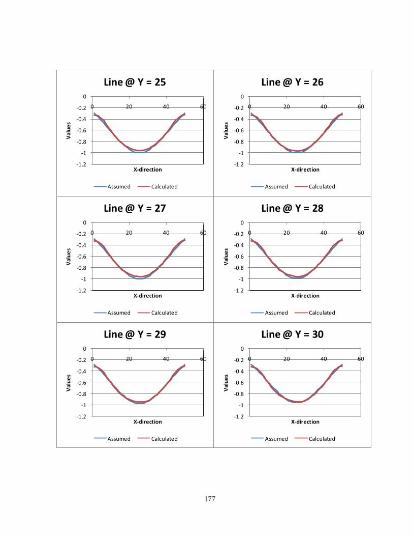
177

-1.2

-1

-0.8

-0.6

-0.4

-0.2

0

0 20 40 60

Val

ue

s

X-direction

Line @ Y = 25

Assumed Calculated

-1.2

-1

-0.8

-0.6

-0.4

-0.2

0

0 20 40 60

Val

ue

s

X-direction

Line @ Y = 26

Assumed Calculated

-1.2

-1

-0.8

-0.6

-0.4

-0.2

0

0 20 40 60

Val

ue

s

X-direction

Line @ Y = 27

Assumed Calculated

-1.2

-1

-0.8

-0.6

-0.4

-0.2

0

0 20 40 60V

alu

es

X-direction

Line @ Y = 28

Assumed Calculated

-1.2

-1

-0.8

-0.6

-0.4

-0.2

0

0 20 40 60

Val

ue

s

X-direction

Line @ Y = 29

Assumed Calculated

-1.2

-1

-0.8

-0.6

-0.4

-0.2

0

0 20 40 60

Val

ue

s

X-direction

Line @ Y = 30

Assumed Calculated

178

Cas19:

Tilt1+2+Displacement, 0%err Omitting 9.2% of points (250) RMSE=0.024057

-0.4

-0.3

-0.2

-0.1

0

0 20 40 60

Val

ue

s

X-direction

Line @ Y = 1

Assumed Calculated

-0.4

-0.3

-0.2

-0.1

0

0 20 40 60

Val

ue

s

X-direction

Line @ Y = 2

Assumed Calculated

-0.4

-0.3

-0.2

-0.1

0

0 20 40 60

Val

ue

s

X-direction

Line @ Y = 3

Assumed Calculated

-0.5

-0.4

-0.3

-0.2

-0.1

0

0 20 40 60

Val

ue

s

X-direction

Line @ Y = 4

Assumed Calculated

-0.5

-0.4

-0.3

-0.2

-0.1

0

0 20 40 60

Val

ue

s

X-direction

Line @ Y = 5

Assumed Calculated

-0.5

-0.4

-0.3

-0.2

-0.1

0

0 20 40 60

Val

ue

s

X-direction

Line @ Y = 6

Assumed Calculated

179

-1.2

-1

-0.8

-0.6

-0.4

-0.2

0

0 20 40 60

Val

ue

s

X-direction

Line @ Y = 25

Assumed Calculated

-1.2

-1

-0.8

-0.6

-0.4

-0.2

0

0 20 40 60

Val

ue

s

X-direction

Line @ Y = 26

Assumed Calculated

-1.2

-1

-0.8

-0.6

-0.4

-0.2

0

0 20 40 60

Val

ue

s

X-direction

Line @ Y = 27

Assumed Calculated

-1.2

-1

-0.8

-0.6

-0.4

-0.2

0

0 20 40 60

Val

ue

s

X-direction

Line @ Y = 28

Assumed Calculated

-1.2

-1

-0.8

-0.6

-0.4

-0.2

0

0 20 40 60

Val

ue

s

X-direction

Line @ Y = 29

Assumed Calculated

-1.2

-1

-0.8

-0.6

-0.4

-0.2

0

0 20 40 60

Val

ue

s

X-direction

Line @ Y = 30

Assumed Calculated

180

Case20:

Tilit1+2+displacement,0%err Omitting 18.5% of points(500)

RMSE=0.024514

-0.4

-0.3

-0.2

-0.1

0

0 20 40 60

Val

ue

s

X-direction

Line @ Y = 1

Assumed Calculated

-0.4

-0.3

-0.2

-0.1

0

0 20 40 60

Val

ue

s

X-direction

Line @ Y = 2

Assumed Calculated

-0.4

-0.3

-0.2

-0.1

0

0 20 40 60

Val

ue

s

X-direction

Line @ Y = 3

Assumed Calculated

-0.5

-0.4

-0.3

-0.2

-0.1

0

0 20 40 60

Val

ue

s

X-direction

Line @ Y = 4

Assumed Calculated

-0.5

-0.4

-0.3

-0.2

-0.1

0

0 20 40 60

Val

ue

s

X-direction

Line @ Y = 5

Assumed Calculated

-0.5

-0.4

-0.3

-0.2

-0.1

0

0 20 40 60

Val

ue

s

X-direction

Line @ Y = 6

Assumed Calculated

181

-1.2

-1

-0.8

-0.6

-0.4

-0.2

0

0 20 40 60

Val

ue

s

X-direction

Line @ Y = 25

Assumed Calculated

-1.2

-1

-0.8

-0.6

-0.4

-0.2

0

0 20 40 60

Val

ue

s

X-direction

Line @ Y = 26

Assumed Calculated

-1.2

-1

-0.8

-0.6

-0.4

-0.2

0

0 20 40 60

Val

ue

s

X-direction

Line @ Y = 27

Assumed Calculated

-1.2

-1

-0.8

-0.6

-0.4

-0.2

0

0 20 40 60V

alu

es

X-direction

Line @ Y = 28

Assumed Calculated

-1.2

-1

-0.8

-0.6

-0.4

-0.2

0

0 20 40 60

Val

ue

s

X-direction

Line @ Y = 29

Assumed Calculated

-1.2

-1

-0.8

-0.6

-0.4

-0.2

0

0 20 40 60

Val

ue

s

X-direction

Line @ Y = 30

Assumed Calculated

182

Case21:

Tilt1+2+displacement,0%err omitting 37% of points(1000)

RMSE=0.029051

-0.4

-0.3

-0.2

-0.1

0

0 20 40 60

Val

ue

s

X-direction

Line @ Y = 1

Assumed Calculated

-0.4

-0.3

-0.2

-0.1

0

0 20 40 60

Val

ue

s

X-direction

Line @ Y = 2

Assumed Calculated

-0.4

-0.3

-0.2

-0.1

0

0 20 40 60

Val

ue

s

X-direction

Line @ Y = 3

Assumed Calculated

-0.5

-0.4

-0.3

-0.2

-0.1

0

0 20 40 60

Val

ue

s

X-direction

Line @ Y = 4

Assumed Calculated

-0.5

-0.4

-0.3

-0.2

-0.1

0

0 20 40 60

Val

ue

s

X-direction

Line @ Y = 5

Assumed Calculated

-0.5

-0.4

-0.3

-0.2

-0.1

0

0 20 40 60

Val

ue

s

X-direction

Line @ Y = 6

Assumed Calculated

183

-1.2

-1

-0.8

-0.6

-0.4

-0.2

0

0 20 40 60

Val

ue

s

X-direction

Line @ Y = 25

Assumed Calculated

-1.2

-1

-0.8

-0.6

-0.4

-0.2

0

0 20 40 60

Val

ue

s

X-direction

Line @ Y = 26

Assumed Calculated

-1.2

-1

-0.8

-0.6

-0.4

-0.2

0

0 20 40 60

Val

ue

s

X-direction

Line @ Y = 27

Assumed Calculated

-1.2

-1

-0.8

-0.6

-0.4

-0.2

0

0 20 40 60

Val

ue

s

X-direction

Line @ Y = 28

Assumed Calculated

-1.2

-1

-0.8

-0.6

-0.4

-0.2

0

0 20 40 60

Val

ue

s

X-direction

Line @ Y = 29

Assumed Calculated

-1.2

-1

-0.8

-0.6

-0.4

-0.2

0

0 20 40 60

Val

ue

s

X-direction

Line @ Y = 30

Assumed Calculated

184

Case 22

Tilit1+2+displacement,0%err omitting 55.5% of points(1500)

RMSE=0.026517

-0.4

-0.3

-0.2

-0.1

0

0 20 40 60

Val

ue

s

X-direction

Line @ Y = 1

Assumed Calculated

-0.4

-0.3

-0.2

-0.1

0

0 20 40 60

Val

ue

s

X-direction

Line @ Y = 2

Assumed Calculated

-0.4

-0.3

-0.2

-0.1

0

0 20 40 60

Val

ue

s

X-direction

Line @ Y = 3

Assumed Calculated

-0.5

-0.4

-0.3

-0.2

-0.1

0

0 20 40 60

Val

ue

s

X-direction

Line @ Y = 4

Assumed Calculated

-0.5

-0.4

-0.3

-0.2

-0.1

0

0 20 40 60

Val

ue

s

X-direction

Line @ Y = 5

Assumed Calculated

-0.5

-0.4

-0.3

-0.2

-0.1

0

0 20 40 60

Val

ue

s

X-direction

Line @ Y = 6

Assumed Calculated

185

-1.2

-1

-0.8

-0.6

-0.4

-0.2

0

0 20 40 60

Val

ue

s

X-direction

Line @ Y = 25

Assumed Calculated

-1.2

-1

-0.8

-0.6

-0.4

-0.2

0

0 20 40 60

Val

ue

s

X-direction

Line @ Y = 26

Assumed Calculated

-1.2

-1

-0.8

-0.6

-0.4

-0.2

0

0 20 40 60

Val

ue

s

X-direction

Line @ Y = 27

Assumed Calculated

-1.2

-1

-0.8

-0.6

-0.4

-0.2

0

0 20 40 60

Val

ue

s

X-direction

Line @ Y = 28

Assumed Calculated

-1.2

-1

-0.8

-0.6

-0.4

-0.2

0

0 20 40 60

Val

ue

s

X-direction

Line @ Y = 29

Assumed Calculated

-1.2

-1

-0.8

-0.6

-0.4

-0.2

0

0 20 40 60

Val

ue

s

X-direction

Line @ Y = 30

Assumed Calculated

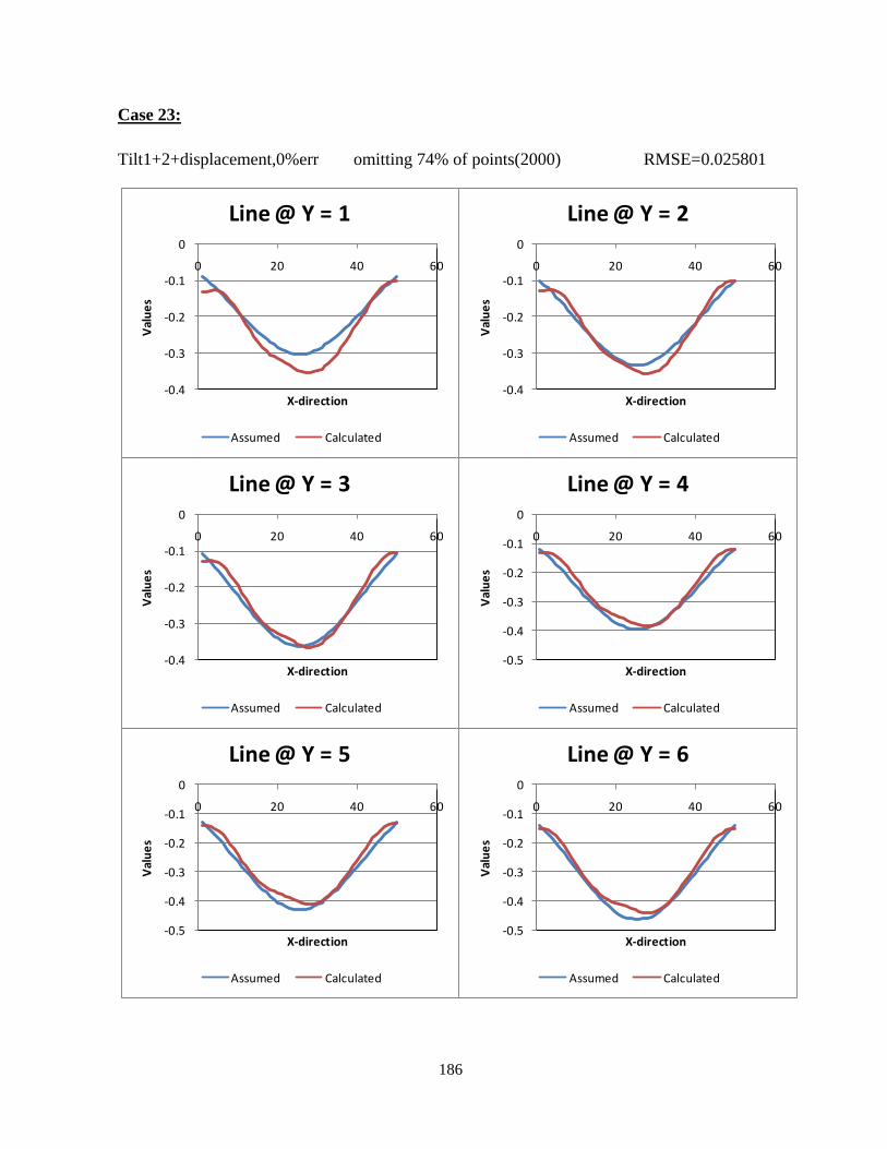
186

Case 23:

Tilt1+2+displacement,0%err omitting 74% of points(2000) RMSE=0.025801

-0.4

-0.3

-0.2

-0.1

0

0 20 40 60

Val

ue

s

X-direction

Line @ Y = 1

Assumed Calculated

-0.4

-0.3

-0.2

-0.1

0

0 20 40 60

Val

ue

s

X-direction

Line @ Y = 2

Assumed Calculated

-0.4

-0.3

-0.2

-0.1

0

0 20 40 60

Val

ue

s

X-direction

Line @ Y = 3

Assumed Calculated

-0.5

-0.4

-0.3

-0.2

-0.1

0

0 20 40 60

Val

ue

s

X-direction

Line @ Y = 4

Assumed Calculated

-0.5

-0.4

-0.3

-0.2

-0.1

0

0 20 40 60

Val

ue

s

X-direction

Line @ Y = 5

Assumed Calculated

-0.5

-0.4

-0.3

-0.2

-0.1

0

0 20 40 60

Val

ue

s

X-direction

Line @ Y = 6

Assumed Calculated

187

-1.2

-1

-0.8

-0.6

-0.4

-0.2

0

0 20 40 60

Val

ue

s

X-direction

Line @ Y = 25

Assumed Calculated

-1.2

-1

-0.8

-0.6

-0.4

-0.2

0

0 20 40 60

Val

ue

s

X-direction

Line @ Y = 26

Assumed Calculated

-1.2

-1

-0.8

-0.6

-0.4

-0.2

0

0 20 40 60

Val

ue

s

X-direction

Line @ Y = 27

Assumed Calculated

-1.2

-1

-0.8

-0.6

-0.4

-0.2

0

0 20 40 60

Val

ue

s

X-direction

Line @ Y = 28

Assumed Calculated

-1.2

-1

-0.8

-0.6

-0.4

-0.2

0

0 20 40 60

Val

ue

s

X-direction

Line @ Y = 29

Assumed Calculated

-1.2

-1

-0.8

-0.6

-0.4

-0.2

0

0 20 40 60

Val

ue

s

X-direction

Line @ Y = 30

Assumed Calculated

188

Case 24:

Tilts1+2+Displacements,0%err Omitting 83% of points(2250) RMSE=0.036212

-0.4

-0.3

-0.2

-0.1

0

0 20 40 60

Val

ue

s

X-direction

Line @ Y = 1

Assumed Calculated

-0.4

-0.3

-0.2

-0.1

0

0 20 40 60

Val

ue

s

X-direction

Line @ Y = 2

Assumed Calculated

-0.4

-0.3

-0.2

-0.1

0

0 20 40 60

Val

ue

s

X-direction

Line @ Y = 3

Assumed Calculated

-0.5

-0.4

-0.3

-0.2

-0.1

0

0 20 40 60

Val

ue

s

X-direction

Line @ Y = 4

Assumed Calculated

-0.5

-0.4

-0.3

-0.2

-0.1

0

0 20 40 60

Val

ue

s

X-direction

Line @ Y = 5

Assumed Calculated

-0.5

-0.4

-0.3

-0.2

-0.1

0

0 20 40 60

Val

ue

s

X-direction

Line @ Y = 6

Assumed Calculated

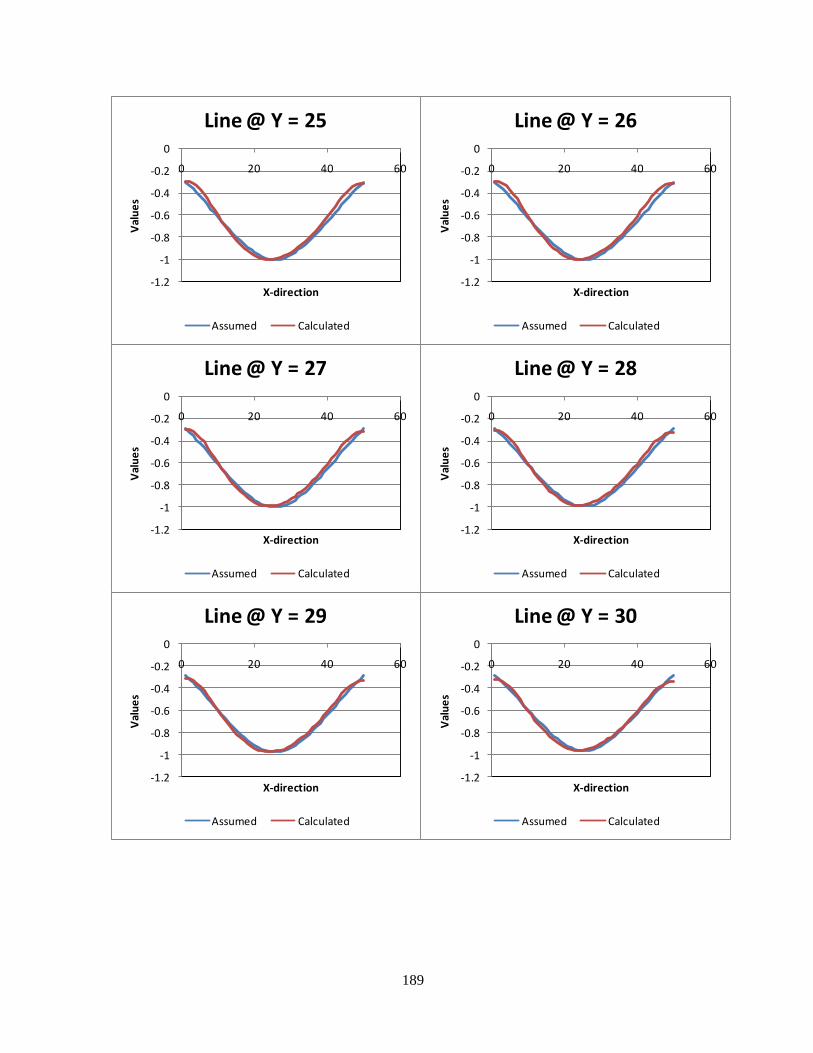
189

-1.2

-1

-0.8

-0.6

-0.4

-0.2

0

0 20 40 60

Val

ue

s

X-direction

Line @ Y = 25

Assumed Calculated

-1.2

-1

-0.8

-0.6

-0.4

-0.2

0

0 20 40 60

Val

ue

s

X-direction

Line @ Y = 26

Assumed Calculated

-1.2

-1

-0.8

-0.6

-0.4

-0.2

0

0 20 40 60

Val

ue

s

X-direction

Line @ Y = 27

Assumed Calculated

-1.2

-1

-0.8

-0.6

-0.4

-0.2

0

0 20 40 60

Val

ue

s

X-direction

Line @ Y = 28

Assumed Calculated

-1.2

-1

-0.8

-0.6

-0.4

-0.2

0

0 20 40 60

Val

ue

s

X-direction

Line @ Y = 29

Assumed Calculated

-1.2

-1

-0.8

-0.6

-0.4

-0.2

0

0 20 40 60

Val

ue

s

X-direction

Line @ Y = 30

Assumed Calculated

190

Case 25:

Tilt1+2+displacement,0%err omitting 89% of points(2400) RMSE=0.041741

-0.5

-0.4

-0.3

-0.2

-0.1

0

0 20 40 60

Val

ue

s

X-direction

Line @ Y = 1

Assumed Calculated

-0.5

-0.4

-0.3

-0.2

-0.1

0

0 20 40 60

Val

ue

s

X-direction

Line @ Y = 2

Assumed Calculated

-0.5

-0.4

-0.3

-0.2

-0.1

0

0 20 40 60

Val

ue

s

X-direction

Line @ Y = 3

Assumed Calculated

-0.5

-0.4

-0.3

-0.2

-0.1

0

0 20 40 60

Val

ue

s

X-direction

Line @ Y = 4

Assumed Calculated

-0.5

-0.4

-0.3

-0.2

-0.1

0

0 20 40 60

Val

ue

s

X-direction

Line @ Y = 5

Assumed Calculated

-0.5

-0.4

-0.3

-0.2

-0.1

0

0 20 40 60

Val

ue

s

X-direction

Line @ Y = 6

Assumed Calculated

191

-1.2

-1

-0.8

-0.6

-0.4

-0.2

0

0 20 40 60

Val

ue

s

X-direction

Line @ Y = 25

Assumed Calculated

-1.2

-1

-0.8

-0.6

-0.4

-0.2

0

0 20 40 60

Val

ue

s

X-direction

Line @ Y = 26

Assumed Calculated

-1.2

-1

-0.8

-0.6

-0.4

-0.2

0

0 20 40 60

Val

ue

s

X-direction

Line @ Y = 27

Assumed Calculated

-1.2

-1

-0.8

-0.6

-0.4

-0.2

0

0 20 40 60

Val

ue

s

X-direction

Line @ Y = 28

Assumed Calculated

-1.2

-1

-0.8

-0.6

-0.4

-0.2

0

0 20 40 60

Val

ue

s

X-direction

Line @ Y = 29

Assumed Calculated

-1.2

-1

-0.8

-0.6

-0.4

-0.2

0

0 20 40 60

Val

ue

s

X-direction

Line @ Y = 30

Assumed Calculated

192

Case 26:

Tilt1+2+Displacement, 0%err omitting 90.6% of data points (2450) RMSE=0.042006

-0.5

-0.4

-0.3

-0.2

-0.1

0

0 20 40 60

Val

ue

s

X-direction

Line @ Y = 1

Assumed Calculated

-0.5

-0.4

-0.3

-0.2

-0.1

0

0 20 40 60

Val

ue

s

X-direction

Line @ Y = 2

Assumed Calculated

-0.5

-0.4

-0.3

-0.2

-0.1

0

0 20 40 60

Val

ue

s

X-direction

Line @ Y = 3

Assumed Calculated

-0.5

-0.4

-0.3

-0.2

-0.1

0

0 20 40 60

Val

ue

s

X-direction

Line @ Y = 4

Assumed Calculated

-0.5

-0.4

-0.3

-0.2

-0.1

0

0 20 40 60

Val

ue

s

X-direction

Line @ Y = 5

Assumed Calculated

-0.5

-0.4

-0.3

-0.2

-0.1

0

0 20 40 60

Val

ue

s

X-direction

Line @ Y = 6

Assumed Calculated

193

-1.2

-1

-0.8

-0.6

-0.4

-0.2

0

0 20 40 60

Val

ue

s

X-direction

Line @ Y = 25

Assumed Calculated

-1.2

-1

-0.8

-0.6

-0.4

-0.2

0

0 20 40 60

Val

ue

s

X-direction

Line @ Y = 26

Assumed Calculated

-1.2

-1

-0.8

-0.6

-0.4

-0.2

0

0 20 40 60

Val

ue

s

X-direction

Line @ Y = 27

Assumed Calculated

-1.2

-1

-0.8

-0.6

-0.4

-0.2

0

0 20 40 60

Val

ue

s

X-direction

Line @ Y = 28

Assumed Calculated

-1.2

-1

-0.8

-0.6

-0.4

-0.2

0

0 20 40 60

Val

ue

s

X-direction

Line @ Y = 29

Assumed Calculated

-1.2

-1

-0.8

-0.6

-0.4

-0.2

0

0 20 40 60

Val

ue

s

X-direction

Line @ Y = 30

Assumed Calculated

194

Case 27:

Tilt1+2+Displacement, 0%error omitting 99.6% of data points (using only 10 random points)

RMSE=0.070773

-0.6

-0.5

-0.4

-0.3

-0.2

-0.1

0

0 20 40 60

Val

ue

s

X-direction

Line @ Y = 1

Assumed Calculated

-0.6

-0.5

-0.4

-0.3

-0.2

-0.1

0

0 20 40 60

Val

ue

s

X-direction

Line @ Y = 2

Assumed Calculated

-0.6

-0.5

-0.4

-0.3

-0.2

-0.1

0

0 20 40 60

Val

ue

s

X-direction

Line @ Y = 3

Assumed Calculated

-0.6

-0.5

-0.4

-0.3

-0.2

-0.1

0

0 20 40 60

Val

ue

s

X-direction

Line @ Y = 4

Assumed Calculated

-0.6

-0.5

-0.4

-0.3

-0.2

-0.1

0

0 20 40 60

Val

ue

s

X-direction

Line @ Y = 5

Assumed Calculated

-0.6

-0.5

-0.4

-0.3

-0.2

-0.1

0

0 20 40 60

Val

ue

s

X-direction

Line @ Y = 6

Assumed Calculated

195

-1.2

-1

-0.8

-0.6

-0.4

-0.2

0

0 20 40 60

Val

ue

s

X-direction

Line @ Y = 25

Assumed Calculated

-1.2

-1

-0.8

-0.6

-0.4

-0.2

0

0 20 40 60

Val

ue

s

X-direction

Line @ Y = 26

Assumed Calculated

-1.2

-1

-0.8

-0.6

-0.4

-0.2

0

0 20 40 60

Val

ue

s

X-direction

Line @ Y = 27

Assumed Calculated

-1.2

-1

-0.8

-0.6

-0.4

-0.2

0

0 20 40 60

Val

ue

s

X-direction

Line @ Y = 28

Assumed Calculated

-1.2

-1

-0.8

-0.6

-0.4

-0.2

0

0 20 40 60

Val

ue

s

X-direction

Line @ Y = 29

Assumed Calculated

-1.2

-1

-0.8

-0.6

-0.4

-0.2

0

0 20 40 60

Val

ue

s

X-direction

Line @ Y = 30

Assumed Calculated

196

Case28:

Tilt1+2+Displacements, 0% err Using 1 point outside the grid RMSE=0.238201

-0.8

-0.6

-0.4

-0.2

0

0 20 40 60

Val

ue

s

X-direction

Line @ Y = 1

Assumed Calculated

-0.8

-0.6

-0.4

-0.2

0

0 20 40 60

Val

ue

s

X-direction

Line @ Y = 2

Assumed Calculated

-0.8

-0.6

-0.4

-0.2

0

0 20 40 60

Val

ue

s

X-direction

Line @ Y = 3

Assumed Calculated

-0.8

-0.6

-0.4

-0.2

0

0 20 40 60

Val

ue

s

X-direction

Line @ Y = 4

Assumed Calculated

-0.8

-0.6

-0.4

-0.2

0

0 20 40 60

Val

ue

s

X-direction

Line @ Y = 5

Assumed Calculated

-0.8

-0.6

-0.4

-0.2

0

0 20 40 60

Val

ue

s

X-direction

Line @ Y = 6

Assumed Calculated

197

-1.2

-1

-0.8

-0.6

-0.4

-0.2

0

0 20 40 60

Val

ue

s

X-direction

Line @ Y = 25

Assumed Calculated

-1.2

-1

-0.8

-0.6

-0.4

-0.2

0

0 20 40 60

Val

ue

s

X-direction

Line @ Y = 26

Assumed Calculated

-1.2

-1

-0.8

-0.6

-0.4

-0.2

0

0 20 40 60

Val

ue

s

X-direction

Line @ Y = 27

Assumed Calculated

-1.2

-1

-0.8

-0.6

-0.4

-0.2

0

0 20 40 60

Val

ue

s

X-direction

Line @ Y = 28

Assumed Calculated

-1.2

-1

-0.8

-0.6

-0.4

-0.2

0

0 20 40 60

Val

ue

s

X-direction

Line @ Y = 29

Assumed Calculated

-1.2

-1

-0.8

-0.6

-0.4

-0.2

0

0 20 40 60

Val

ue

s

X-direction

Line @ Y = 30

Assumed Calculated

198

Appendix V: Graphs; studying the effect of observation distribution

Case29:Tilt1+2+Displ,0%err, using 100points at 1 vertical and 1horizontal rows at corners of

grid: X,Y=5 5<X,Y<495 RMSE=0.04958528

-0.5

-0.4

-0.3

-0.2

-0.1

0

0 20 40 60

Val

ue

s

X-direction

Line @ Y = 1

Assumed Calculated

-0.5

-0.4

-0.3

-0.2

-0.1

0

0 20 40 60

Val

ue

s

X-direction

Line @ Y = 2

Assumed Calculated

-0.5

-0.4

-0.3

-0.2

-0.1

0

0 20 40 60

Val

ue

s

X-direction

Line @ Y = 3

Assumed Calculated

-0.5

-0.4

-0.3

-0.2

-0.1

0

0 20 40 60

Val

ue

s

X-direction

Line @ Y = 4

Assumed Calculated

-0.5

-0.4

-0.3

-0.2

-0.1

0

0 20 40 60

Val

ue

s

X-direction

Line @ Y = 5

Assumed Calculated

-0.5

-0.4

-0.3

-0.2

-0.1

0

0 20 40 60

Val

ue

s

X-direction

Line @ Y = 6

Assumed Calculated

199

-1.2

-1

-0.8

-0.6

-0.4

-0.2

0

0 20 40 60

Val

ue

s

X-direction

Line @ Y = 25

Assumed Calculated

-1.2

-1

-0.8

-0.6

-0.4

-0.2

0

0 20 40 60

Val

ue

s

X-direction

Line @ Y = 26

Assumed Calculated

-1.2

-1

-0.8

-0.6

-0.4

-0.2

0

0 20 40 60

Val

ue

s

X-direction

Line @ Y = 27

Assumed Calculated

-1.2

-1

-0.8

-0.6

-0.4

-0.2

0

0 20 40 60

Val

ue

s

X-direction

Line @ Y = 28

Assumed Calculated

-1.2

-1

-0.8

-0.6

-0.4

-0.2

0

0 20 40 60

Val

ue

s

X-direction

Line @ Y = 29

Assumed Calculated

-1.2

-1

-0.8

-0.6

-0.4

-0.2

0

0 20 40 60

Val

ue

s

X-direction

Line @ Y = 30

Assumed Calculated

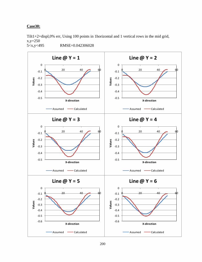
200

Case30:

Tilt1+2+displ,0% err, Using 100 points in 1horizontal and 1 vertical rows in the mid grid,

x,y=250

5<x,y<495 RMSE=0.042306028

-0.5

-0.4

-0.3

-0.2

-0.1

0

0 20 40 60

Val

ue

s

X-direction

Line @ Y = 1

Assumed Calculated

-0.5

-0.4

-0.3

-0.2

-0.1

0

0 20 40 60

Val

ue

s

X-direction

Line @ Y = 2

Assumed Calculated

-0.5

-0.4

-0.3

-0.2

-0.1

0

0 20 40 60

Val

ue

s

X-direction

Line @ Y = 3

Assumed Calculated

-0.5

-0.4

-0.3

-0.2

-0.1

0

0 20 40 60

Val

ue

s

X-direction

Line @ Y = 4

Assumed Calculated

-0.6

-0.5

-0.4

-0.3

-0.2

-0.1

0

0 20 40 60

Val

ue

s

X-direction

Line @ Y = 5

Assumed Calculated

-0.6

-0.5

-0.4

-0.3

-0.2

-0.1

0

0 20 40 60

Val

ue

s

X-direction

Line @ Y = 6

Assumed Calculated

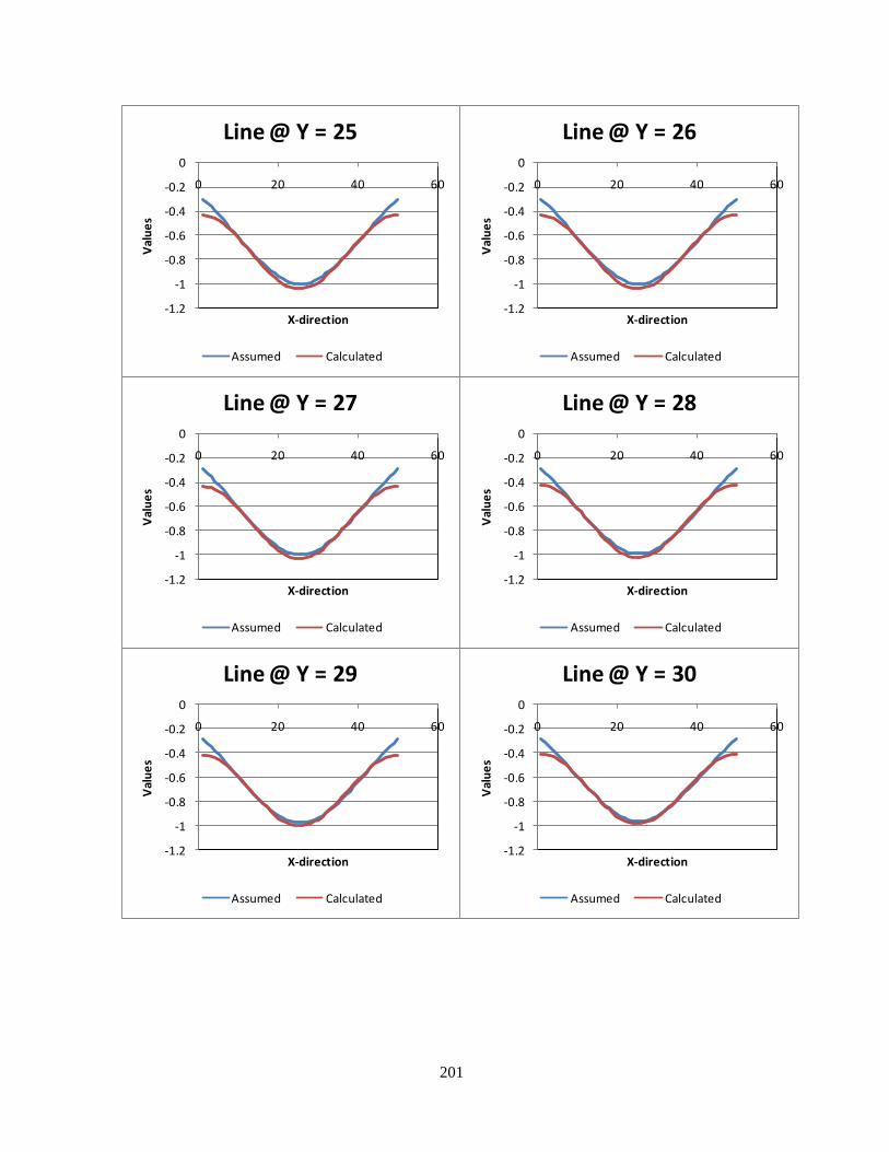
201

-1.2

-1

-0.8

-0.6

-0.4

-0.2

0

0 20 40 60

Val

ue

s

X-direction

Line @ Y = 25

Assumed Calculated

-1.2

-1

-0.8

-0.6

-0.4

-0.2

0

0 20 40 60

Val

ue

s

X-direction

Line @ Y = 26

Assumed Calculated

-1.2

-1

-0.8

-0.6

-0.4

-0.2

0

0 20 40 60

Val

ue

s

X-direction

Line @ Y = 27

Assumed Calculated

-1.2

-1

-0.8

-0.6

-0.4

-0.2

0

0 20 40 60

Val

ue

s

X-direction

Line @ Y = 28

Assumed Calculated

-1.2

-1

-0.8

-0.6

-0.4

-0.2

0

0 20 40 60

Val

ue

s

X-direction

Line @ Y = 29

Assumed Calculated

-1.2

-1

-0.8

-0.6

-0.4

-0.2

0

0 20 40 60

Val

ue

s

X-direction

Line @ Y = 30

Assumed Calculated

202

Case31:

Tilt1+2+displ,0%err,Using 100 extended points(-500<x,y<1000) in 1vertical and 1 horizontal

rows in the mid grid(X,Y=250) RMSE=0.043834347

-0.5

-0.4

-0.3

-0.2

-0.1

0

0 20 40 60

Val

ue

s

X-direction

Line @ Y = 1

Assumed Calculated

-0.5

-0.4

-0.3

-0.2

-0.1

0

0 20 40 60

Val

ue

s

X-direction

Line @ Y = 2

Assumed Calculated

-0.5

-0.4

-0.3

-0.2

-0.1

0

0 20 40 60

Val

ue

s

X-direction

Line @ Y = 3

Assumed Calculated

-0.5

-0.4

-0.3

-0.2

-0.1

0

0 20 40 60

Val

ue

s

X-direction

Line @ Y = 4

Assumed Calculated

-0.6

-0.5

-0.4

-0.3

-0.2

-0.1

0

0 20 40 60

Val

ue

s

X-direction

Line @ Y = 5

Assumed Calculated

-0.6

-0.5

-0.4

-0.3

-0.2

-0.1

0

0 20 40 60

Val

ue

s

X-direction

Line @ Y = 6

Assumed Calculated

203

-1.2

-1

-0.8

-0.6

-0.4

-0.2

0

0 20 40 60

Val

ue

s

X-direction

Line @ Y = 25

Assumed Calculated

-1.2

-1

-0.8

-0.6

-0.4

-0.2

0

0 20 40 60

Val

ue

s

X-direction

Line @ Y = 26

Assumed Calculated

-1.2

-1

-0.8

-0.6

-0.4

-0.2

0

0 20 40 60

Val

ue

s

X-direction

Line @ Y = 27

Assumed Calculated

-1.2

-1

-0.8

-0.6

-0.4

-0.2

0

0 20 40 60

Val

ue

s

X-direction

Line @ Y = 28

Assumed Calculated

-1.2

-1

-0.8

-0.6

-0.4

-0.2

0

0 20 40 60

Val

ue

s

X-direction

Line @ Y = 29

Assumed Calculated

-1.2

-1

-0.8

-0.6

-0.4

-0.2

0

0 20 40 60

Val

ue

s

X-direction

Line @ Y = 30

Assumed Calculated

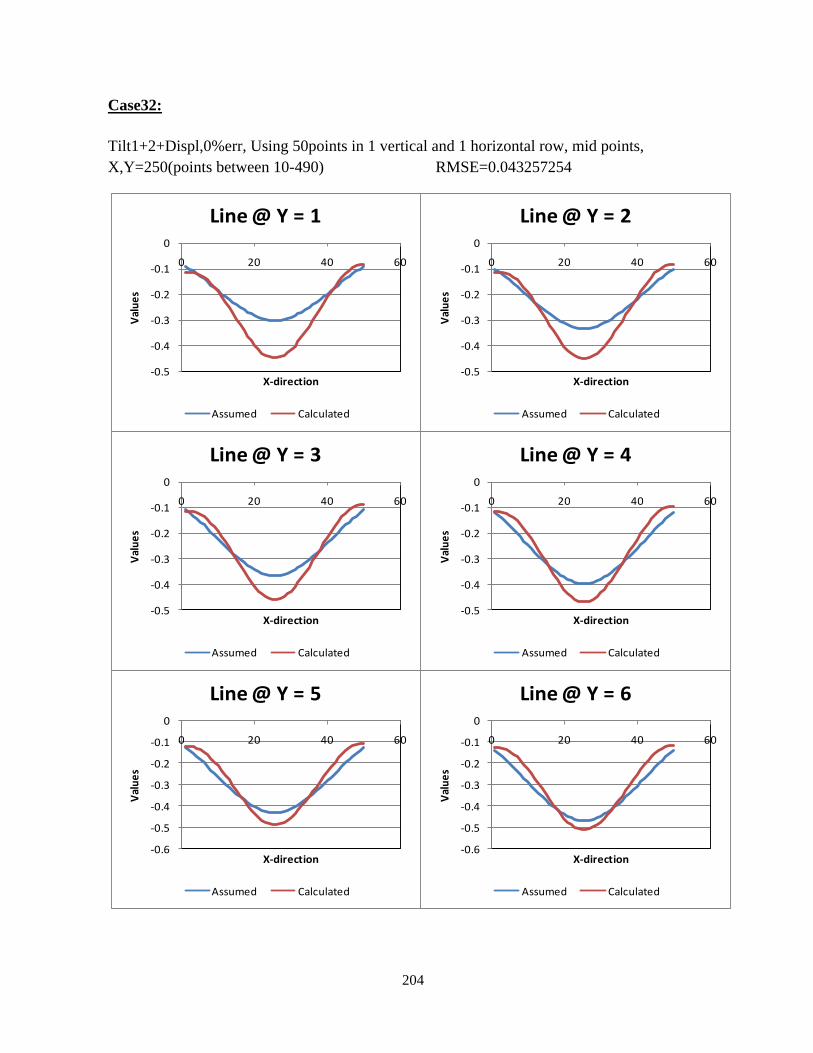
204

Case32:

Tilt1+2+Displ,0%err, Using 50points in 1 vertical and 1 horizontal row, mid points,

X,Y=250(points between 10-490) RMSE=0.043257254

-0.5

-0.4

-0.3

-0.2

-0.1

0

0 20 40 60

Val

ue

s

X-direction

Line @ Y = 1

Assumed Calculated

-0.5

-0.4

-0.3

-0.2

-0.1

0

0 20 40 60

Val

ue

s

X-direction

Line @ Y = 2

Assumed Calculated

-0.5

-0.4

-0.3

-0.2

-0.1

0

0 20 40 60

Val

ue

s

X-direction

Line @ Y = 3

Assumed Calculated

-0.5

-0.4

-0.3

-0.2

-0.1

0

0 20 40 60

Val

ue

s

X-direction

Line @ Y = 4

Assumed Calculated

-0.6

-0.5

-0.4

-0.3

-0.2

-0.1

0

0 20 40 60

Val

ue

s

X-direction

Line @ Y = 5

Assumed Calculated

-0.6

-0.5

-0.4

-0.3

-0.2

-0.1

0

0 20 40 60

Val

ue

s

X-direction

Line @ Y = 6

Assumed Calculated

205

-1.2

-1

-0.8

-0.6

-0.4

-0.2

0

0 20 40 60

Val

ue

s

X-direction

Line @ Y = 25

Assumed Calculated

-1.2

-1

-0.8

-0.6

-0.4

-0.2

0

0 20 40 60

Val

ue

s

X-direction

Line @ Y = 26

Assumed Calculated

-1.2

-1

-0.8

-0.6

-0.4

-0.2

0

0 20 40 60

Val

ue

s

X-direction

Line @ Y = 27

Assumed Calculated

-1.2

-1

-0.8

-0.6

-0.4

-0.2

0

0 20 40 60

Val

ue

s

X-direction

Line @ Y = 28

Assumed Calculated

-1.2

-1

-0.8

-0.6

-0.4

-0.2

0

0 20 40 60

Val

ue

s

X-direction

Line @ Y = 29

Assumed Calculated

-1.2

-1

-0.8

-0.6

-0.4

-0.2

0

0 20 40 60

Val

ue

s

X-direction

Line @ Y = 30

Assumed Calculated

206

Case33:

Tilt1+2+displ, 0%err Using 10points in 1 vertical and 1 horizontal points, mid points of the

grid X,Y=250

5<x,y<495 RMSE=0.047407172

-0.5

-0.4

-0.3

-0.2

-0.1

0

0 20 40 60

Val

ue

s

X-direction

Line @ Y = 1

Assumed Calculated

-0.5

-0.4

-0.3

-0.2

-0.1

0

0 20 40 60

Val

ue

s

X-direction

Line @ Y = 2

Assumed Calculated

-0.5

-0.4

-0.3

-0.2

-0.1

0

0 20 40 60

Val

ue

s

X-direction

Line @ Y = 3

Assumed Calculated

-0.5

-0.4

-0.3

-0.2

-0.1

0

0 20 40 60

Val

ue

s

X-direction

Line @ Y = 4

Assumed Calculated

-0.6

-0.5

-0.4

-0.3

-0.2

-0.1

0

0 20 40 60

Val

ue

s

X-direction

Line @ Y = 5

Assumed Calculated

-0.6

-0.5

-0.4

-0.3

-0.2

-0.1

0

0 20 40 60

Val

ue

s

X-direction

Line @ Y = 6

Assumed Calculated

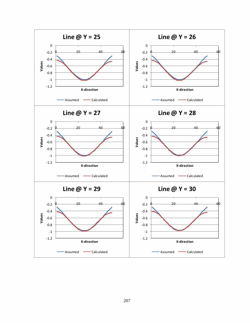
207

-1.2

-1

-0.8

-0.6

-0.4

-0.2

0

0 20 40 60

Val

ue

s

X-direction

Line @ Y = 25

Assumed Calculated

-1.2

-1

-0.8

-0.6

-0.4

-0.2

0

0 20 40 60

Val

ue

s

X-direction

Line @ Y = 26

Assumed Calculated

-1.2

-1

-0.8

-0.6

-0.4

-0.2

0

0 20 40 60

Val

ue

s

X-direction

Line @ Y = 27

Assumed Calculated

-1.2

-1

-0.8

-0.6

-0.4

-0.2

0

0 20 40 60

Val

ue

s

X-direction

Line @ Y = 28

Assumed Calculated

-1.2

-1

-0.8

-0.6

-0.4

-0.2

0

0 20 40 60

Val

ue

s

X-direction

Line @ Y = 29

Assumed Calculated

-1.2

-1

-0.8

-0.6

-0.4

-0.2

0

0 20 40 60

Val

ue

s

X-direction

Line @ Y = 30

Assumed Calculated

208

Case34:

Tilt1+2 10%err, Using1000 points in 1 vertical and 1 horizontal rows,-500<x,y<1000

RMSE=0.318229

-1

-0.5

0

0.5

1

0 20 40 60

Val

ue

s

X-direction

Line @ Y = 1

Assumed Calculated

-1

-0.5

0

0.5

1

0 20 40 60

Val

ue

s

X-direction

Line @ Y = 2

Assumed Calculated

-1

-0.5

0

0.5

1

0 20 40 60

Val

ue

s

X-direction

Line @ Y = 3

Assumed Calculated

-1

-0.5

0

0.5

1

0 20 40 60

Val

ue

s

X-direction

Line @ Y = 4

Assumed Calculated

-1

-0.5

0

0.5

1

0 20 40 60

Val

ue

s

X-direction

Line @ Y = 5

Assumed Calculated

-1.5

-1

-0.5

0

0.5

1

0 20 40 60

Val

ue

s

X-direction

Line @ Y = 6

Assumed Calculated

209

-1.5

-1

-0.5

0

0 20 40 60

Val

ue

s

X-direction

Line @ Y = 25

Assumed Calculated

-1.2

-1

-0.8

-0.6

-0.4

-0.2

0

0 20 40 60

Val

ue

s

X-direction

Line @ Y = 26

Assumed Calculated

-1.2

-1

-0.8

-0.6

-0.4

-0.2

0

0 20 40 60

Val

ue

s

X-direction

Line @ Y = 27

Assumed Calculated

-1.2

-1

-0.8

-0.6

-0.4

-0.2

0

0 20 40 60

Val

ue

s

X-direction

Line @ Y = 28

Assumed Calculated

-1.2

-1

-0.8

-0.6

-0.4

-0.2

0

0 20 40 60

Val

ue

s

X-direction

Line @ Y = 29

Assumed Calculated

-1.2

-1

-0.8

-0.6

-0.4

-0.2

0

0 20 40 60

Val

ue

s

X-direction

Line @ Y = 30

Assumed Calculated

210

Case 35:

Tilt1+2,10% err, Using300 points in 1vertical and 1horizontal rows, -500<x,y<1000

RMSE=0.3297

-1.5

-1

-0.5

0

0.5

1

0 20 40 60

Val

ue

s

X-direction

Line @ Y = 1

Assumed Calculated

-1.5

-1

-0.5

0

0.5

1

0 20 40 60

Val

ue

s

X-direction

Line @ Y = 2

Assumed Calculated

-1.5

-1

-0.5

0

0.5

1

0 20 40 60

Val

ue

s

X-direction

Line @ Y = 3

Assumed Calculated

-1.5

-1

-0.5

0

0.5

1

0 20 40 60

Val

ue

s

X-direction

Line @ Y = 4

Assumed Calculated

-1.5

-1

-0.5

0

0.5

1

0 20 40 60

Val

ue

s

X-direction

Line @ Y = 5

Assumed Calculated

-1.5

-1

-0.5

0

0.5

1

0 20 40 60

Val

ue

s

X-direction

Line @ Y = 6

Assumed Calculated

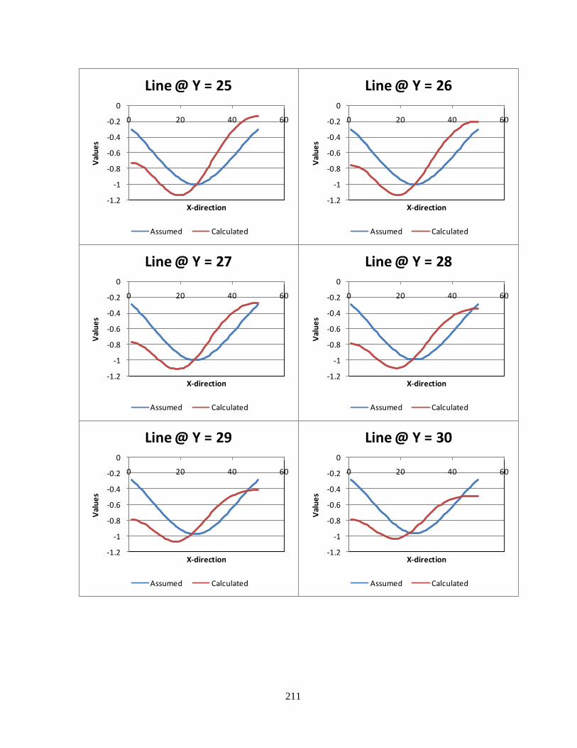
211

-1.2

-1

-0.8

-0.6

-0.4

-0.2

0

0 20 40 60

Val

ue

s

X-direction

Line @ Y = 25

Assumed Calculated

-1.2

-1

-0.8

-0.6

-0.4

-0.2

0

0 20 40 60

Val

ue

s

X-direction

Line @ Y = 26

Assumed Calculated

-1.2

-1

-0.8

-0.6

-0.4

-0.2

0

0 20 40 60

Val

ue

s

X-direction

Line @ Y = 27

Assumed Calculated

-1.2

-1

-0.8

-0.6

-0.4

-0.2

0

0 20 40 60

Val

ue

s

X-direction

Line @ Y = 28

Assumed Calculated

-1.2

-1

-0.8

-0.6

-0.4

-0.2

0

0 20 40 60

Val

ue

s

X-direction

Line @ Y = 29

Assumed Calculated

-1.2

-1

-0.8

-0.6

-0.4

-0.2

0

0 20 40 60

Val

ue

s

X-direction

Line @ Y = 30

Assumed Calculated

212

Case 36:

Tilt1+2, 10%err Using 300points in 1 horizontal & 1 vertical row 0<X,Y<500

RMSE=0.328058

-0.4

-0.2

0

0.2

0.4

0.6

0 20 40 60

Val

ue

s

X-direction

Line @ Y = 1

Assumed Calculated

-0.4

-0.2

0

0.2

0.4

0.6

0 20 40 60

Val

ue

s

X-direction

Line @ Y = 2

Assumed Calculated

-0.6

-0.4

-0.2

0

0.2

0.4

0.6

0 20 40 60

Val

ue

s

X-direction

Line @ Y = 3

Assumed Calculated

-0.6

-0.4

-0.2

0

0.2

0.4

0.6

0 20 40 60

Val

ue

s

X-direction

Line @ Y = 4

Assumed Calculated

-0.6

-0.4

-0.2

0

0.2

0.4

0.6

0 20 40 60

Val

ue

s

X-direction

Line @ Y = 5

Assumed Calculated

-0.6

-0.4

-0.2

0

0.2

0.4

0.6

0 20 40 60

Val

ue

s

X-direction

Line @ Y = 6

Assumed Calculated

213

-1.5

-1

-0.5

0

0 20 40 60

Val

ue

s

X-direction

Line @ Y = 25

Assumed Calculated

-1.5

-1

-0.5

0

0 20 40 60

Val

ue

s

X-direction

Line @ Y = 26

Assumed Calculated

-1.5

-1

-0.5

0

0 20 40 60

Val

ue

s

X-direction

Line @ Y = 27

Assumed Calculated

-1.2

-1

-0.8

-0.6

-0.4

-0.2

0

0 20 40 60

Val

ue

s

X-direction

Line @ Y = 28

Assumed Calculated

-1.2

-1

-0.8

-0.6

-0.4

-0.2

0

0 20 40 60

Val

ue

s

X-direction

Line @ Y = 29

Assumed Calculated

-1.2

-1

-0.8

-0.6

-0.4

-0.2

0

0 20 40 60

Val

ue

s

X-direction

Line @ Y = 30

Assumed Calculated

214

Case37:

Tilt1+2, 10%err Using300points in 3 horizontal,3 vertical rows

RMSE=0.291543

-0.6

-0.4

-0.2

0

0.2

0.4

0.6

0.8

0 20 40 60

Val

ue

s

X-direction

Line @ Y = 1

Assumed Calculated

-0.6

-0.4

-0.2

0

0.2

0.4

0.6

0.8

0 20 40 60

Val

ue

s

X-direction

Line @ Y = 2

Assumed Calculated

-0.5

0

0.5

1

0 20 40 60

Val

ue

s

X-direction

Line @ Y = 3

Assumed Calculated

-0.5

0

0.5

1

0 20 40 60

Val

ue

s

X-direction

Line @ Y = 4

Assumed Calculated

-1

-0.5

0

0.5

1

0 20 40 60

Val

ue

s

X-direction

Line @ Y = 5

Assumed Calculated

-1

-0.5

0

0.5

1

0 20 40 60

Val

ue

s

X-direction

Line @ Y = 6

Assumed Calculated

215

-1.5

-1

-0.5

0

0 20 40 60

Val

ue

s

X-direction

Line @ Y = 25

Assumed Calculated

-1.5

-1

-0.5

0

0 20 40 60

Val

ue

s

X-direction

Line @ Y = 26

Assumed Calculated

-1.5

-1

-0.5

0

0 20 40 60

Val

ue

s

X-direction

Line @ Y = 27

Assumed Calculated

-1.2

-1

-0.8

-0.6

-0.4

-0.2

0

0 20 40 60

Val

ue

s

X-direction

Line @ Y = 28

Assumed Calculated

-1.2

-1

-0.8

-0.6

-0.4

-0.2

0

0.2

0 20 40 60

Val

ue

s

X-direction

Line @ Y = 29

Assumed Calculated

-1.2

-1

-0.8

-0.6

-0.4

-0.2

0

0.2

0 20 40 60

Val

ue

s

X-direction

Line @ Y = 30

Assumed Calculated

216

Case38:

300points,3 vertical,3 horizontal rows,100m spacing between rows,10% err

RMSE=0.339687

-1

-0.5

0

0.5

1

0 20 40 60

Val

ue

s

X-direction

Line @ Y = 1

Assumed Calculated

-1

-0.5

0

0.5

1

0 20 40 60

Val

ue

s

X-direction

Line @ Y = 2

Assumed Calculated

-1

-0.5

0

0.5

1

0 20 40 60

Val

ue

s

X-direction

Line @ Y = 3

Assumed Calculated

-1

-0.5

0

0.5

1

0 20 40 60

Val

ue

s

X-direction

Line @ Y = 4

Assumed Calculated

-1

-0.5

0

0.5

1

0 20 40 60

Val

ue

s

X-direction

Line @ Y = 5

Assumed Calculated

-1

-0.5

0

0.5

1

0 20 40 60

Val

ue

s

X-direction

Line @ Y = 6

Assumed Calculated

217

-1.5

-1

-0.5

0

0 20 40 60

Val

ue

s

X-direction

Line @ Y = 25

Assumed Calculated

-1.5

-1

-0.5

0

0 20 40 60

Val

ue

s

X-direction

Line @ Y = 26

Assumed Calculated

-1.5

-1

-0.5

0

0 20 40 60

Val

ue

s

X-direction

Line @ Y = 27

Assumed Calculated

-1.2

-1

-0.8

-0.6

-0.4

-0.2

0

0 20 40 60

Val

ue

s

X-direction

Line @ Y = 28

Assumed Calculated

-1.2

-1

-0.8

-0.6

-0.4

-0.2

0

0 20 40 60

Val

ue

s

X-direction

Line @ Y = 29

Assumed Calculated

-1.2

-1

-0.8

-0.6

-0.4

-0.2

0

0 20 40 60

Val

ue

s

X-direction

Line @ Y = 30

Assumed Calculated

218

Case39:

300 points 6Vertical rows of 50, 10% err, Tilt1+2 RMSE=0.222957

-0.6

-0.4

-0.2

0

0.2

0.4

0.6

0 20 40 60

Val

ue

s

X-direction

Line @ Y = 1

Assumed Calculated

-0.6

-0.4

-0.2

0

0.2

0.4

0.6

0 20 40 60

Val

ue

s

X-direction

Line @ Y = 2

Assumed Calculated

-0.6

-0.4

-0.2

0

0.2

0.4

0.6

0 20 40 60

Val

ue

s

X-direction

Line @ Y = 3

Assumed Calculated

-0.6

-0.4

-0.2

0

0.2

0.4

0.6

0 20 40 60

Val

ue

s

X-direction

Line @ Y = 4

Assumed Calculated

-0.6

-0.4

-0.2

0

0.2

0.4

0.6

0 20 40 60

Val

ue

s

X-direction

Line @ Y = 5

Assumed Calculated

-0.8

-0.6

-0.4

-0.2

0

0.2

0.4

0.6

0 20 40 60Val

ue

s

X-direction

Line @ Y = 6

Assumed Calculated

219

-1.5

-1

-0.5

0

0 20 40 60

Val

ue

s

X-direction

Line @ Y = 25

Assumed Calculated

-1.5

-1

-0.5

0

0 20 40 60

Val

ue

s

X-direction

Line @ Y = 26

Assumed Calculated

-1.5

-1

-0.5

0

0 20 40 60

Val

ue

s

X-direction

Line @ Y = 27

Assumed Calculated

-1.5

-1

-0.5

0

0 20 40 60

Val

ue

s

X-direction

Line @ Y = 28

Assumed Calculated

-1.5

-1

-0.5

0

0 20 40 60

Val

ue

s

X-direction

Line @ Y = 29

Assumed Calculated

-1.5

-1

-0.5

0

0 20 40 60

Val

ue

s

X-direction

Line @ Y = 30

Assumed Calculated

220

Case 40:

Tilt1+2 , 10%err Using 300 points in 2 vertical rows 0<x,y<500 RMSE=0.271487

-1

-0.5

0

0.5

1

0 20 40 60

Val

ue

s

X-direction

Line @ Y = 1

Assumed Calculated

-1

-0.5

0

0.5

1

0 20 40 60

Val

ue

s

X-direction

Line @ Y = 2

Assumed Calculated

-1

-0.5

0

0.5

1

0 20 40 60

Val

ue

s

X-direction

Line @ Y = 3

Assumed Calculated

-1

-0.5

0

0.5

1

0 20 40 60

Val

ue

s

X-direction

Line @ Y = 4

Assumed Calculated

-1

-0.5

0

0.5

1

0 20 40 60

Val

ue

s

X-direction

Line @ Y = 5

Assumed Calculated

-0.6

-0.4

-0.2

0

0.2

0.4

0.6

0.8

0 20 40 60

Val

ue

s

X-direction

Line @ Y = 6

Assumed Calculated

221

-1.5

-1

-0.5

0

0.5

0 20 40 60

Val

ue

s

X-direction

Line @ Y = 25

Assumed Calculated

-2

-1.5

-1

-0.5

0

0.5

0 20 40 60

Val

ue

s

X-direction

Line @ Y = 26

Assumed Calculated

-2

-1.5

-1

-0.5

0

0.5

0 20 40 60

Val

ue

s

X-direction

Line @ Y = 27

Assumed Calculated

-2

-1.5

-1

-0.5

0

0.5

0 20 40 60V

alu

es

X-direction

Line @ Y = 28

Assumed Calculated

-2

-1.5

-1

-0.5

0

0.5

0 20 40 60

Val

ue

s

X-direction

Line @ Y = 29

Assumed Calculated

-2

-1.5

-1

-0.5

0

0.5

0 20 40 60

Val

ue

s

X-direction

Line @ Y = 30

Assumed Calculated

222

Case41:

Tilt1+2,10%err, Using 100 points in 1 horizontal and 1 vertical row 0<x,y<500

RMSE=0.375072

-1

-0.5

0

0.5

1

1.5

0 20 40 60

Val

ue

s

X-direction

Line @ Y = 1

Assumed Calculated

-1

-0.5

0

0.5

1

1.5

0 20 40 60

Val

ue

s

X-direction

Line @ Y = 2

Assumed Calculated

-1

-0.5

0

0.5

1

1.5

0 20 40 60

Val

ue

s

X-direction

Line @ Y = 3

Assumed Calculated

-1

-0.5

0

0.5

1

1.5

0 20 40 60

Val

ue

s

X-direction

Line @ Y = 4

Assumed Calculated

-1

-0.5

0

0.5

1

1.5

0 20 40 60

Val

ue

s

X-direction

Line @ Y = 5

Assumed Calculated

-1

-0.5

0

0.5

1

0 20 40 60

Val

ue

s

X-direction

Line @ Y = 6

Assumed Calculated

223

-1.5

-1

-0.5

0

0 20 40 60

Val

ue

s

X-direction

Line @ Y = 25

Assumed Calculated

-1.5

-1

-0.5

0

0 20 40 60

Val

ue

s

X-direction

Line @ Y = 26

Assumed Calculated

-1.5

-1

-0.5

0

0 20 40 60

Val

ue

s

X-direction

Line @ Y = 27

Assumed Calculated

-1.5

-1

-0.5

0

0 20 40 60

Val

ue

s

X-direction

Line @ Y = 28

Assumed Calculated

-1.2

-1

-0.8

-0.6

-0.4

-0.2

0

0 20 40 60

Val

ue

s

X-direction

Line @ Y = 29

Assumed Calculated

-1.2

-1

-0.8

-0.6

-0.4

-0.2

0

0 20 40 60

Val

ue

s

X-direction

Line @ Y = 30

Assumed Calculated

224

Case42:

Tilt1+2, 5%err Using300 points in 6 rows RMSE=0.116004

-0.6

-0.4

-0.2

0

0.2

0 20 40 60

Val

ue

s

X-direction

Line @ Y = 1

Assumed Calculated

-0.6

-0.4

-0.2

0

0.2

0 20 40 60

Val

ue

s

X-direction

Line @ Y = 2

Assumed Calculated

-0.6

-0.4

-0.2

0

0.2

0 20 40 60

Val

ue

s

X-direction

Line @ Y = 3

Assumed Calculated

-0.6

-0.4

-0.2

0

0.2

0 20 40 60

Val

ue

s

X-direction

Line @ Y = 4

Assumed Calculated

-0.6

-0.4

-0.2

0

0.2

0 20 40 60

Val

ue

s

X-direction

Line @ Y = 5

Assumed Calculated

-0.6

-0.4

-0.2

0

0.2

0 20 40 60

Val

ue

s

X-direction

Line @ Y = 6

Assumed Calculated

225

-1.5

-1

-0.5

0

0 20 40 60

Val

ue

s

X-direction

Line @ Y = 25

Assumed Calculated

-1.5

-1

-0.5

0

0 20 40 60

Val

ue

s

X-direction

Line @ Y = 26

Assumed Calculated

-1.5

-1

-0.5

0

0 20 40 60

Val

ue

s

X-direction

Line @ Y = 27

Assumed Calculated

-1.2

-1

-0.8

-0.6

-0.4

-0.2

0

0 20 40 60

Val

ue

s

X-direction

Line @ Y = 28

Assumed Calculated

-1.2

-1

-0.8

-0.6

-0.4

-0.2

0

0 20 40 60

Val

ue

s

X-direction

Line @ Y = 29

Assumed Calculated

-1.2

-1

-0.8

-0.6

-0.4

-0.2

0

0 20 40 60

Val

ue

s

X-direction

Line @ Y = 30

Assumed Calculated

226

Case43:

Tilt1+2-3%err Using 300points at 6 vertical rows RMSE=0.080343

-0.6

-0.4

-0.2

0

0.2

0 20 40 60

Val

ue

s

X-direction

Line @ Y = 1

Assumed Calculated

-0.6

-0.4

-0.2

0

0.2

0 20 40 60

Val

ue

s

X-direction

Line @ Y = 2

Assumed Calculated

-0.6

-0.4

-0.2

0

0.2

0 20 40 60

Val

ue

s

X-direction

Line @ Y = 3

Assumed Calculated

-0.6

-0.4

-0.2

0

0.2

0 20 40 60

Val

ue

s

X-direction

Line @ Y = 4

Assumed Calculated

-0.6

-0.4

-0.2

0

0.2

0 20 40 60

Val

ue

s

X-direction

Line @ Y = 5

Assumed Calculated

-0.6

-0.4

-0.2

0

0.2

0 20 40 60

Val

ue

s

X-direction

Line @ Y = 6

Assumed Calculated

227

-1.2

-1

-0.8

-0.6

-0.4

-0.2

0

0 20 40 60

Val

ue

s

X-direction

Line @ Y = 25

Assumed Calculated

-1.2

-1

-0.8

-0.6

-0.4

-0.2

0

0 20 40 60

Val

ue

s

X-direction

Line @ Y = 26

Assumed Calculated

-1.2

-1

-0.8

-0.6

-0.4

-0.2

0

0 20 40 60

Val

ue

s

X-direction

Line @ Y = 27

Assumed Calculated

-1.2

-1

-0.8

-0.6

-0.4

-0.2

0

0 20 40 60V

alu

es

X-direction

Line @ Y = 28

Assumed Calculated

-1.2

-1

-0.8

-0.6

-0.4

-0.2

0

0 20 40 60

Val

ue

s

X-direction

Line @ Y = 29

Assumed Calculated

-1.2

-1

-0.8

-0.6

-0.4

-0.2

0

0 20 40 60

Val

ue

s

X-direction

Line @ Y = 30

Assumed Calculated

228

Appendix VI: the numerical modeling of the inverse solution in C++

The Coding of the direct and inverse solution: #include<iostream>

#include<fstream>

#include<iomanip>

#include<cstdio>

#include<math.h>

#include<time.h>

#include <stdio.h>

using namespace std;

void okadadisp(double x,double y,double z,double e,double d,double dip,double sn,double cs,double prt, double

a[3]);

void okadatilt(double x,double y,double z,double e,double d,double dip,double sn,double cs,double prt,double

tss[5],double tds[5],double tts[5]);

void calculation(double ,double ,double ,double ,double ,double ,double ,double , double ,double ,double ,double ,

double* ,double* ,double* ,double* ,double* ,double*,double*);

void laplace(double dx,double N,int nx,int ny,double **lap,double **L);

void SVDcmp(int,int,double **KL,float **u,float **s,float **vT,float w[3600],float **v);

void svbksb(float **u,float w[3600],float **v,int m,int n,float b[3600],float x[3600]);

void main()

{

double dx,dy,FL,FW,XF4,YF4,disS[4],disD[4],disT[4],Tstrike[4],Tdip[4],Ttensile[4];

double disstrike,disdip,distensile,TStrike[4],TDip[4],TT[4];

double l,W,Dx,Dy,XO,YO,depth, dip,asim, depthr,dtr,umd4,ums4,umv4,Xmin,Xmax,Ymin,Ymax;

int i,j,nx,ny,k,m,Nx,Ny,El;

double U1[3600],U2[3600];

int obser,el,o,F;

double 𝛽;

int NX,NY;

float **u,**s,**vT,**v;

float w[3600],Answer[3600],volume[3600];

int NO;

double UMV[3600],Err[3600],std,Var;

double kk[4];

double KK[4];

double Xobser[3000],Yobser[3000];

double Aa;

double TTerror1[2],TTerror2[2];

double RR;

time_t start, stop;

clock_t ticks; long count;

time(&start);

double ** K1,**K2,**L,**lap,**A,**KL;

K1 = new double*[3600];

for (i=0;i<=3600;i++)

K1[i]=new double[3600];

K2 = new double*[3600];

for (i=0;i<=3600;i++)

K2[i]=new double[3600];

L = new double*[3600];

229

for (i=0;i<=3600;i++)

L[i]=new double[3600];

lap = new double*[3600];

for (i=0;i<=3600;i++)

lap[i]=new double[3600];

A = new double*[3600];

for (i=0;i<=3600;i++)

A[i]=new double[3600];

KL = new double*[3600];

for (i=0;i<=3600;i++)

KL[i]=new double[3600];

u = new float*[3600];

for (i=0;i<=3600;i++)

u[i]=new float[3600];

s = new float*[3600];

for (i=0;i<=3600;i++)

s[i]=new float[3600];

vT = new float*[3600];

for (i=0;i<=3600;i++)

vT[i]=new float[3600];

v = new float*[3600];

for (i=0;i<=3600;i++)

v[i]=new float[3600];

𝛽=0.0000001; ///𝛽 is the calibration factor for invers

dtr = 3.1415926/180;

umd4=0;

ums4=0;

umv4=-1;

nx=51; //No of reservior nodes

ny=51;

FL=500;

FW=500;

depth=500;

dip=0;

asim =0;

dx=FL/(nx-1);

dy=FW/(ny-1);

//reservior elements

El=(nx-1)*(ny-1);

NX=nx-1; ///No of reservior elements in X direction

NY=ny-1; ///No of reservior elements in Y direction

Nx=50; //No of observation points in x direction

Ny=50;

//Dx=10;

//Dy=10;

//Dx=(Xmax-Xmin)/(Nx-1);

//Dy=(Ymax-Ymin)/(Ny-1);

disstrike=0;

TT[1]=0;

TT[2]=0;

disdip=0;

distensile=0;

TStrike[1]=0;

230

TStrike[2]=0;

TDip[1]=0;

TDip[2]=0;

////////// OBSERVATION POINTS//////

ofstream fout;

fout.open("test.txt");

o=Nx*Ny;

obser=0;

el=0;

Aa=1+depth/(FL/2);

//////////////for observation points grid with respect to depth//////

Xobser[0]=Aa*(0-FL/2)+FL/2;

Yobser[0]=Aa*(0-FL/2)+FL/2;

Xobser[Nx+1]=Aa*(FL-FL/2)+FL/2;

Yobser[Ny+1]=Aa*(FL-FL/2)+FL/2;

for(i=1;i<=2500;++i){

XF4=(i-1)*dx+dx/2; //RESERVIOR POINTS

YF4=(i-1)*dy*cos(dip*dtr)+dy/2;

Xobser[i]=Aa*(XF4-FL/2)+FL/2;

Yobser[i]=Aa*(YF4-FL/2)+FL/2;

cout<<"OBSERVATION POINT"<<Xobser[i]<<" "<<Yobser[i]<<"\n";}

fout<<"OBSERVATION POINT: "<<"\n";

for(k=0;k<=Nx+1;++k)

{

for(m=0;m<=Ny+1;++m)

{

NO=0;

obser=obser+1;

el=0;

//XO=Xmin+(k-1)*Dx;

//YO=Ymin+(m-1)*Dy;

XO=Xobser[k];

YO=Yobser[m];

disstrike=0;

TT[1]=0;

TT[2]=0;

disdip=0;

distensile=0;

TStrike[1]=0;

TStrike[2]=0;

TDip[1]=0;

TDip[2]=0;

cout<<"OBSERVATION POINT: "<<XO<<" "<<YO<<"\n";

for (i=1;i<=nx-1;++i)

{

for (j=1;j<=(ny-1);++j)

{

NO=NO+1;

XF4=(i-1)*dx+dx/2; //RESERVIOR POINTS

YF4=(j-1)*dy*cos(dip*dtr);

231

depthr = depth - dy*(j-1)*sin(dip*dtr);

umv4=-exp(-(((XF4-FL/2)*(XF4-FL/2)+(YF4+dy/2-FW/2)*(YF4+dy/2-FW/2)))/(100*FL));

UMV[NO]=umv4; Volume change assigned to each reservoir element:

calculation(XO,YO,XF4,YF4,dy,dx,depthr,dip,asim,umd4,ums4,umv4,disS,disD,disT,Tstrike,Tdip,Ttensile,KK);

disstrike=disS[1]+disstrike;

disdip=disD[1]+disdip;

el=el+1;

K1[obser][el]=KK[1];

K2[obser][el]=KK[2];

distensile=disT[1]+distensile;

TStrike[1]=Tstrike[1]+TStrike[1];

TStrike[2]=Tstrike[2]+TStrike[2];

TDip[1]=Tdip[1]+TDip[1];

TDip[2]=Tdip[2]+TDip[2];

TT[1]=Ttensile[1]+TT[1];

TT[2]=Ttensile[2]+TT[2];

///////////For random generator to consider error

RR=rand()%(10)+1;

RR=6.341*0.00001*RR/10;

TTerror1[1]=TT[1]+RR;

TTerror2[1]=TT[2]+RR;

////for U tilt matrix: (input data with error for inverse solution)

U1[obser]=TTerror1[1];

U2[obser]=TTerror2[1];

}

}

fout<<XO<<","<<YO<<","<<distensile<<"\n";

fout<<"TILT1 of X Y with error and Tilt2= "<<TTerror1[1]<<" "<<TTerror2[1]<<"\n";

cout<<"disp strike ="<<disstrike<<"\n";

cout<<"disp dip ="<<disdip<<"\n";

cout<<"disp tilt ="<<distensile<<"\n";

cout<<"tilt S x ="<<TStrike[1]<<"\n";

cout<<"tilt s y ="<<TStrike[2]<<"\n";

cout<<"tilt D x ="<<TDip[1]<<"\n";

cout<<"tilt D y ="<<TDip[2]<<"\n";

cout<<"tilt t x ="<<TT[1]<<"\n";

cout<<"tilt t y ="<<TT[2]<<"\n";

}

}

fout.close();

fout.open("test2.txt");

for (i=1;i<=El;i++)

for (j=1;j<=El;j++)

A[i][j]=0;

for (i=1;i<=El;i++){

for (j=1;j<=El;j++){

for (F=0;F<=o-1;F++){

if (i<=j){

A[i][j]=A[i][j]+K1[1+F][i]*K1[1+F][j]+K2[1+F][i]*K2[1+F][j];}

else

A[i][j]=A[j][i];}

}

}

232

cout<<"//////////////////////////////////////////////////"<<"\n";

laplace(dx,El,NX,NY,lap,L);

for (i=1;i<=El;i++)

{

for(j=1;j<=El;j++)

{

KL[i][j]=A[i][j]-𝛽*L[i][j];}

}


Answer[i]=0;}


for (j=1;j<=o;j++){

Answer[i]+=K1[j][i]*U1[j]+K2[j][i]*U2[j];}

}

SVDcmp(El,El,KL,u,s,vT,w,v);

///for calculating volume

svbksb(u,w,v,El,El,Answer,volume);

cout<<"initial Volume="<<"\n";

fout<<"initial Volume="<<"\n";

for(i=1;i<=El;i++){

cout<<UMV[i]<<"\n";

fout<<UMV[i]<<"\n";

}

cout<<" Volume="<<"\n";

fout<<" Volume="<<"\n";

for(i=1;i<=El;i++){

cout<<volume[i]<<"\n";

fout<<volume[i]<<"\n";

}

cout<<"NO="<<NO<<"\n";

fout<<"NO="<<NO<<"\n";

////////////error calculation:

cout<<"Error%="<<"\n";

fout<<"Error%="<<"\n";

for(i=1;i<=El;i++){

Err[i]=(UMV[i]-volume[i])*100/UMV[i];

cout<<Err[i]<<"\n";

fout<<Err[i]<<"\n";

}

////calculating MSE and RMSE:

Var=0;

for(i=1;i<=El;i++)

{

Var=Var+(UMV[i]-volume[i])*(UMV[i]-volume[i]);

}

Var=Var/El;

std=sqrt(Var);

time(&stop);

cout<<"MSE"<<Var<<"\n";

cout<<"RMSE"<<std<<"\n";

fout<<"MSE"<<Var<<"\n";

233

fout<<"RMSE"<<std<<"\n";

printf("Finished in about %.0f seconds. \n", difftime(stop, start));

fout.close();

}

///////////////////////////////////////////////////////////////////////////////////////////////////////////////

void calculation(double Xo4,double Yo4,double Xf,double Yf,double fw4,double fl4,double depth4, double dip4,

double asim4,double Umd,double Ums,double Umv, double SS[4],double DS[4],double TS[4],double t[3],double

td[3],double tilt[5],double KK[4])

{

double pi,pi2,prt,dtr,asim,dip,d;

double ca,sa,sn,cs,DX,DY,XL,YL,zi,zf,ei,ef,okd1[5],okd2[5],okd3[5],okd4[5];

double ds1,ts1,ss1,disl,ss2,ss3,ss4,ds2,ds3,ds4,ts2,ts3,ts4;

double

tss1[4],tss2[4],tss3[4],tss4[4],tds1[4],tds2[4],tds3[4],tds4[4],tts1[4],tts2[4],tts3[4],tts4[4],Tilt[4],pi2i,disp4;

double kk[5];

int i;

prt=0.5;

pi=3.141592654;

pi2=pi*2;

pi2i=1/pi2;

dtr=pi2/360; //for angle trans

asim=asim4*dtr;

dip=dip4*dtr;

d=depth4;

ca=cos(asim);

sa=sin(asim);

sn=sin(dip);

cs=cos(dip);

DX=Xo4-Xf;

DY=Yo4-Yf;

XL=DX*ca+DY*sa;

YL=-DX*sa+DY*ca;

zi=XL-0.5*fl4;

zf=XL+0.5*fl4;

ei=YL*cs+d*sn;

ef=ei-fw4;

okadadisp(XL,YL,zi,ei,d,dip,sn,cs,prt,okd1);

ss1=okd1[1];

ds1=okd1[2];

ts1=okd1[3];

okadadisp(XL,YL,zi,ef,d,dip,sn,cs,prt,okd2);

ss2=okd2[1];

ds2=okd2[2];

ts2=okd2[3];

okadadisp(XL,YL,zf,ei,d,dip,sn,cs,prt,okd3);

ss3=okd3[1];

ds3=okd3[2];

234

ts3=okd3[3];

okadadisp(XL,YL,zf,ef,d,dip,sn,cs,prt,okd4);

ss4=okd4[1];

ds4=okd4[2];

ts4=okd4[3];

disl=(ss1-ss2-ss3+ss4)*Ums;

SS[1]=disl*pi2i;

disl=disl+(ds1-ds2-ds3+ds4)*Umd;

DS[1]=(ds1-ds2-ds3+ds4)*Umd*pi2i;

disl=disl+(ts1-ts2-ts3+ts4)*Umv;

TS[1]=(ts1-ts2-ts3+ts4)*Umv*pi2i;

disp4=disl*pi2i;

okadatilt(XL,YL,zi,ei,d,dip,sn,cs,prt,tss1,tds1,tts1);

okadatilt(XL,YL,zi,ef,d,dip,sn,cs,prt,tss2,tds2,tts2);

okadatilt(XL,YL,zf,ei,d,dip,sn,cs,prt,tss3,tds3,tts3);

okadatilt(XL,YL,zf,ef,d,dip,sn,cs,prt,tss4,tds4,tts4);

t[1]=(tss1[1]-tss2[1]-tss3[1]+tss4[1])*Ums/pi2;

t[2]=(tss1[2]-tss2[2]-tss3[2]+tss4[2])*Ums/pi2;

td[1]=(tds1[1]-tds2[1]-tds3[1]+tds4[1])*Umd/pi2;

td[2]=(tds1[2]-tds2[2]-tds3[2]+tds4[2])*Umd/pi2;

for(i=1;i<=2;++i){

Tilt[i]=(tss1[i]-tss2[i]-tss3[i]+tss4[i])*Ums;

Tilt[i]=Tilt[i]+(tds1[i]-tds2[i]-tds3[i]+tds4[i])*Umd;

Tilt[i]=Tilt[i]+(tts1[i]-tts2[i]-tts3[i]+tts4[i])*Umv;

kk[i]=tts1[i]-tts2[i]-tts3[i]+tts4[i];

}

KK[1]=(kk[1]*ca-kk[2]*sa)/pi2;

KK[2]=(kk[1]*sa+kk[2]*ca)/pi2;

tilt[1]=(Tilt[1]*ca-Tilt[2]*sa)/pi2;

tilt[2]=(Tilt[1]*sa+Tilt[2]*ca)/pi2;

}

void okadadisp(double x,double y,double z,double e,double d,double dip,double sn,double cs,double prt,double

a[3])

{

double q,dt,yt,rc,xc,rci,rce,rcz,tn,lgt,t4,tn5,td5,t5,tme,tmz,tmzr,tmer,ds,ts,ss;

cs=cos(dip);

sn=sin(dip);

q=y*sn-d*cs;

dt=e*sn-q*cs;

yt=e*cs+q*sn;

rc=sqrt(z*z+e*e+q*q);

xc= sqrt(z*z+q*q);

rci=1/rc;

rce=rc+e;

rcz=rc+z;

if (abs(q)> 0.00001)

tn=atan((z*e)/(q*rc));

else

tn=0;

235

if (abs(cs)>0.00001) {

if (rce>0.00001)

lgt= log(rce);

else

lgt=-log(rc-e);

t4=prt*((log(rc+dt)-sn*lgt)/cs);

if (abs(z)>0.00001)

{

tn5=e*(xc+q*cs)+xc*(rc+xc)*sn;

td5=z*(rc+xc)*cs;

t5=prt*2*atan(tn5/td5)/cs;

}

else

t5=0;

}

if (abs(cs<0.00001)){

t4=-prt*q/(rc+dt);

t5=-prt*z*sn/(rc+dt);

}

if (abs(rce)>0.00001){

tme=q/rce;}

else

tme=0;

if (rcz!=0)

tmz=q/rcz;

else

tmz=0;

tmzr=tmz*rci;

tmer=tme*rci;

ss=-dt*tmer-(tme+t4)*sn;

ds=-dt*tmzr-sn*tn+t5*sn*cs;

ts=yt*tmzr+cs*(z*tmer-tn)-t5*sn*sn;

a[1]=ss;

a[2]=ds;

a[3]=ts;

}

void okadatilt(double x,double y,double z,double e,double d,double dip,double sn,double cs,double prt,double

ss[4],double ds[4],double ts[4])

{

double q,dt,yt,rc,xc,q2,z2,sn2,sncs,r3,re,rz,rd,az,qr3,rrz,rre,ae,trm;

double tk1,tk2,tk3;

cs=cos(dip);

sn=sin(dip);

q=y*sn-d*cs;

dt=e*sn-q*cs;

yt=e*cs+q*sn;

rc=sqrt(z*z+e*e+q*q);

xc= sqrt(z*z+q*q);

236

q2=q*q;

z2=z*z;

sn2=sn*sn;

sncs=sn*cs;

r3=rc*rc*rc;

re=rc+e;

rz=rc+z;

rd=rc+dt;

az=(2*rc+z)/(r3*rz*rz);

qr3=q/r3;

rrz=rc*rz;

rre=rc*re;

if (re>0.00001){

ae=(2*rc+e)/(r3*re*re);

trm=sn/rre;

}

else{

ae=0;

trm=0;

}

if (abs(cs>0.00001)){

tk1=prt*z*(1/(rc*rd)-sn/rre)/cs;

tk3=prt*(q/rre-yt/(rc*rd))/cs;

tk2=prt*(-sn/rc+q*cs/rre)-tk3;

}

else{

tk1=prt*z*q/(rc*rd*rd);

tk3=prt*sn/rd*(z2/(rc*rd)-1);

tk2=prt*(-sn/rc)-tk3;

}

ss[1]=-z*q2*ae*cs+(z*qr3-tk1)*sn;

ss[2]=dt*cs*qr3+(z2*q*ae*cs-sn/rc+yt*qr3-tk2)*sn;

ds[1]=dt*qr3+q*trm+tk3*sncs;

ds[2]=yt*dt*q*az-(2*dt/rrz+z*trm)*sn+tk1*sncs;

ts[1]=-q2*sn/r3+q*q2*ae*cs-tk3*sn2;

ts[2]=-(yt*sn+dt*cs)*q2*az-z*q2*ae*sncs+(2*q/rrz-tk1)*sn2;

}

///for calculating Laplace operator:

void laplace(double h,double N,int nx,int ny,double **l,double **L)

{

int i,j,F;

//for array-matriz:

int k;

double hx,hy;

//N No of reservior elements

//M No of observation points

//hx=1;

for (i=1;i<=N;i++){

for(j=1;j<=N;j++){

l[i][j]=0;}

237

}

for (i=1;i<=N;i++)

{

for(j=1;j<=N;j++)

{

if(i==j)

{l[i][j]=-4/(h*h);}

else{

for (k=1;k<=ny-2;k++){ ///for mid points

if(i>(k*nx+1) && i<(k+1)*nx){

l[i][i-nx]=1/(h*h);

l[i][i-1]=1/(h*h);

l[i][i+1]=1/(h*h);

l[i][i+nx]=1/(h*h);}}

if (i==1){

l[i][i+1]=l[i][i+nx]=2/(h*h);}

if (i==nx){

l[i][i-1]=l[i][i+nx]=2/(h*h);}

if (i==nx*(ny-1)+1 ||i==N){

l[i][i+1]=l[i][i-nx]=2/(h*h);}

if (i==N){

l[i][i-1]=l[i][i-nx]=2/(h*h);

}

}

if(1<i && i<nx){

l[i][i-1]=l[i][i+1]=1/(h*h);

l[i][i+nx]=2/(h*h);}

if((ny-1)*nx+1<i && i<N){

l[i][i-1]=l[i][i+1]=1/(h*h);

l[i][i-nx]=2/(h*h);}

for(k=1;k<ny-1;k++){

if(i==(k+1)*nx){

l[i][i-1]=2/(h*h);

l[i][i+nx]=l[i][i-nx]=1/(h*h);}

else

if(i==k*nx+1){

l[i][i+1]=2/(h*h);

l[i][i+nx]=l[i][i-nx]=1/(h*h);}

}

}

}

for (i=1;i<=N;i++){

for (j=1;j<=N;j++){

L[i][j]=0;

}

}

for (i=1;i<=N;i++)

{

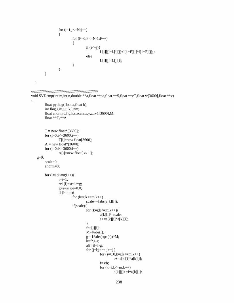
238

for (j=1;j<=N;j++)

{

for (F=0;F<=N-1;F++)

{

if (i<=j){

L[i][j]=L[i][j]+l[1+F][i]*l[1+F][j];}

else

L[i][j]=L[j][i];

}

}

}

}

///////////////////////////////////////////////////////////////

void SVDcmp(int m,int n,double **a,float **aa,float **S,float **vT,float w[3600],float **v)

{

float pythag(float a,float b);

int flag,i,its,j,jj,k,l,nm;

float anorm,c,f,g,h,s,scale,x,y,z,rv1[3600],M;

float **T,**A;

T = new float*[3600];

for (i=0;i<=3600;i++)

T[i]=new float[3600];

A = new float*[3600];

for (i=0;i<=3600;i++)

A[i]=new float[3600];

g=0;

scale=0;

anorm=0;

for (i=1;i<=n;i++){

l=i+1;

rv1[i]=scale*g;

g=s=scale=0.0;

if (i<=m){

for (k=i;k<=m;k++)

scale+=fabs(a[k][i]);

if(scale){

for (k=i;k<=m;k++){

a[k][i]/=scale;

s+=a[k][i]*a[k][i];

}

f=a[i][i];

M=f/abs(f);

g=-1*abs(sqrt(s))*M;

h=f*g-s;

a[i][i]=f-g;

for (j=l;j<=n;j++){

for (s=0.0,k=i;k<=m;k++)

s+=a[k][i]*a[k][j];

f=s/h;

for (k=i;k<=m;k++)

a[k][j]+=f*a[k][i];

239

}

for (k=i;k<=m;k++)

a[k][i]*=scale;

}

}

w[i]=scale*g;

g=s=scale=0.0;

if(i<=m && i!=n){

for (k=l;k<=n;k++)

scale+=fabs(a[i][k]);

if (scale){

for (k=l;k<=n;k++){

a[i][k]/=scale;

s+=a[i][k]*a[i][k];

}

f=a[i][l];

//Replacement for -SIGN function

M=f/abs(f);

g=-1*abs(sqrt(s))*M;

h=f*g-s;

a[i][l]=f-g;

for (k=l;k<=n;k++)

rv1[k]=a[i][k]/h;

for (j=l;j<=m;j++){

for (s=0.0,k=l;k<=n;k++)

s+=a[j][k]*a[i][k];

for (k=l;k<=n;k++)

a[j][k]+=s*rv1[k];

}

for (k=l;k<=n;k++)

a[i][k]*=scale;

}

}

anorm=max(anorm,(fabs(w[i])+fabs(rv1[i])));

}

for(i=n;i>=1;i--){

if (i<n){

if (g){

for (j=l;j<=n;j++)

v[j][i]=(a[i][j]/a[i][l])/g;

for (j=l;j<=n;j++){

for (s=0.0,k=l;k<=n;k++)

s+=a[i][k]*v[k][j];

for (k=l;k<=n;k++)

v[k][j]+=s*v[k][i];

}

}

for (j=l;j<=n;j++)

v[i][j]=v[j][i]=0.0;

}

v[i][i]=1.0;

g=rv1[i];

l=i;

}

240

//Accumulation of left-hand transformations.

for (i=min(m,n);i>=1;i--){

l=i+1;

g=w[i];

for (j=l;j<=n;j++)

a[i][j]=0.0;

if(g){

g=1/g;

for(j=l;j<=n;j++){

for(s=0.0,k=l;k<=m;k++)

s+=a[k][i]*a[k][j];

f=(s/a[i][i])*g;

for (k=i;k<=m;k++)

a[k][j]+=f*a[k][i];

}

for (j=i;j<=m;j++)

a[j][i]*=g;

}

else for (j=i;j<=m;j++)

a[j][i]=0.0;

++a[i][i];

}

//Diagonalization of the bidiagonal form:Loop over singular values,and over allowed iterations

for (k=n;k>=1;k--){

for(its=1;its<=300;its++){

flag=1;

for(l=k;l>=1;l--){

nm=l-1;

if ((float)(fabs(rv1[l])+anorm)==anorm) {

flag=0;

break;

}

if ((float)(fabs(w[nm])+anorm)==anorm)

break;

}

if (flag){ //cancellation of rv1[l],if l>1

c=0.0;

s=1.0;

for (i=l;i<=k;i++){

f=s*rv1[i];

rv1[i]=c*rv1[i];

if((float)(fabs(f)+anorm)==anorm)

break;

g=w[i];

h=pythag(f,g);

w[i]=h;

h=1/h;

c=g*h;

s=-f*h;

for (j=1;j<=m;j++){

y=a[j][nm];

z=a[j][i];

a[j][nm]=y*c+z*s;

a[j][i]=z*c-y*s;

241

}

}

}

z=w[k];

if(l==k){

if(z<0.0){

w[k]=-z;

for (j=1;j<=n;j++)

v[j][k]=-v[j][k];

}

break;

}

if(its==300){ cout<<"not conver"<<"\n";

exit(1);

}

//nrerror("no convergence on 30 svdcmp iterations");

///////shift from bottom 2-by-2 minor//////

x=w[l];

nm=k-1;

y=w[nm];

g=rv1[nm];

h=rv1[k];

f=((y-z)*(y+z)+(g-h)*(g+h))/(2*h*y);

g=pythag(f,1);

//Replacement for -SIGN function

M=f/abs(f);

g=abs(g)*M;

f=((x-z)*(x+z)+h*((y/(f+g))-h))/x;

c=s=1.0;

for (j=l;j<=nm;j++){

i=j+1;

g=rv1[i];

y=w[i];

h=s*g;

g=c*g;

z=pythag(f,h);

rv1[j]=z;

c=f/z;

s=h/z;

f=x*c+g*s;

g=g*c-x*s;

h=y*s;

y *=c;

for (jj=1;jj<=n;jj++){

x=v[jj][j];

z=v[jj][i];

v[jj][j]=x*c+z*s;

v[jj][i]=z*c-x*s;

}

z=pythag(f,h);

w[j]=z;

if (z){

z=1/z;

242

c=f*z;

s=h*z;

}

f=c*g+s*y;

x=c*y-s*g;

for (jj=1;jj<=m;jj++){

y=a[jj][j];

z=a[jj][i];

a[jj][j]=y*c+z*s;

a[jj][i]=z*c-y*s;

}

}

rv1[l]=0;

rv1[k]=f;

w[k]=x;

}

}

for(k=1;k<=m;++k)

{

for(j=1;j<=n;++j)

{

aa[k][j]=a[k][j];}

}

for (i=1;i<=n;++i)

{

for(k=1;k<=n;++k)

{

vT[i][k]=v[k][i];

}

}

cout<<"w[]="<<"\n";

for (i=1;i<=n;i++){

for(j=1;j<=n;j++){

if(i!=j)

S[i][j]=0;

else

S[i][j]=w[i];

}

}

for (i=1;i<=m;i++){

for(j=1;j<=n;j++){

T[i][j]=0;

}

}

for (i=1;i<=n;i++){

for(j=1;j<=n;j++){

for(k=1;k<=n;k++){

T[i][j]+=S[i][k]*vT[k][j];

}

}

}

for (i=1;i<=m;i++){

for(j=1;j<=n;j++){

A[i][j]=0;

}

243

}

for(i=1;i<=m;i++){

for(j=1;j<=n;j++){

for(k=1;k<=n;k++){

A[i][j]+=a[i][k]*T[k][j];

}

}

}

}

float pythag(float a,float b)

//computes (a^2+b^2)^0.5 without destructive underflow or overflow

{

float absa,absb;

absa=fabs(a);

absb=fabs(b);

if(absa>absb)

return absa*sqrt(1+(absb/absa)*(absb/absa));

else

return (absb==0?0 : absb*sqrt(1+(absa/absb)*(absa/absb)));

}

////////////////////////////////////////////////////////////////////////////void svbksb(float **u,float w[3600],float **v,int m,int n,float

b[3600],float x[3600])

{

int jj,j,i;

double s,tmp[3600];

for (j=1;j<=n;j++){ ///calculate UT B

s=0;

if(w[j]){ ///Nonzero result only if wj is nonzero

for(i=1;i<=m;i++)

s+=u[i][j]*b[i];

s/=w[j];

}

tmp[j]=s;

}

for(j=1;j<=n;j++){

s=0; ///Matrix multiply by V to get answer

for(jj=1;jj<=n;jj++)

s+=v[j][jj]*tmp[jj];

x[j]=s;

}

}

monitoring oil reservoir deformations by measuring ground

Documents