monitoring ice break-up on the mackenzie river … ice break-up on the mackenzie river using modis...
TRANSCRIPT
The Cryosphere, 10, 569–584, 2016
www.the-cryosphere.net/10/569/2016/
doi:10.5194/tc-10-569-2016
© Author(s) 2016. CC Attribution 3.0 License.
Monitoring ice break-up on the Mackenzie River using MODIS data
P. Muhammad, C. Duguay, and K.-K. Kang
Department of Geography and the Interdisciplinary Centre on Climate Change (IC3), University of Waterloo,
Waterloo, ON, Canada
Correspondence to: P. Muhammad ([email protected]) and C. Duguay ([email protected])
Received: 20 March 2015 – Published in The Cryosphere Discuss.: 20 May 2015
Revised: 23 November 2015 – Accepted: 1 December 2015 – Published: 11 March 2016
Abstract. The aim of this study was to develop an approach
for estimating ice break-up dates on the Mackenzie River
(MR) using more than a decade of MODIS Level 3 500 m
snow products (MOD/MYD10A1), complemented with
250 m Level 1B radiance products (MOD/MYD02QKM)
from the Terra and Aqua satellite platforms.
The analysis showed break-up began on average between
days of year (DOYs) 115 and 125 and ended between
DOYs 145 and 155 over 13 ice seasons (2001–2013), result-
ing in an average melt duration of ca. 30–40 days. Thermal
processes were more important in driving ice break-up south
of the MR confluence with the Liard River, while dynami-
cally driven break-up was more important north of the Liard.
A comparison of the timing of ice disappearance with
snow disappearance from surrounding land areas of the MR
with MODIS Level 3 snow products showed varying rela-
tionships along the river. Ice-off and snow-off timing were in
sync north of the MR–Liard River confluence and over sec-
tions of the MR before it enters the Mackenzie Delta, but ice
disappeared much later than snow on land in regions where
thermal ice break-up processes dominated.
MODIS observations revealed that channel morphology is
a more important control of ice break-up patterns than previ-
ously believed with ice runs on the MR strongly influenced
by channel morphology (islands and bars, confluences and
channel constriction).
Ice velocity estimates from feature tracking were able to
be made in 2008 and 2010 and yielded 3–4-day average ice
velocities of 1.21 and 1.84 ms−1 respectively, which is in
agreement with estimates from previous studies.
These preliminary results confirm the utility of daily
MODIS data for monitoring ice break-up processes along the
Mackenzie River. The addition of optical and synthetic aper-
ture radar data from recent and upcoming satellite missions
(e.g. Sentinel-1/2/3 and RADARSAT Constellation) would
improve the monitoring of ice break-up in narrower sections
of the MR.
1 Introduction
The Mackenzie River basin (MRB) is the largest in Canada
and is subject to one of the most important annual hydrologic
events. River-ice break-up on the Mackenzie River (MR) is
a process by which upstream (lower latitude) ice is pushed
downstream while intact ice resists movement downstream
(higher latitude) (Beltaos and Prowse, 2009). Ice break-up
is defined as a process with specific dates identifying key
events in space and time between the onset of melt and the
complete disappearance of ice in the river. This is the defi-
nition used in previously published literature and will be ap-
plied in this paper. Break-up is often associated with flood-
ing in north-flowing systems and is thus an important hydro-
logic event with many environmental benefits (e.g. geochem-
ical land deposition and lake and groundwater recharge) and
detriments (e.g. infrastructure damage and lost economic ac-
tivity) (Prowse, 2001; Kääb et al., 2013). Investigations of
river regimes in high-latitude countries including Canada, the
United States, Russia, Sweden and Finland have a long his-
tory related to their ice monitoring (Lenormand et al., 2002).
This is important as ice freeze-up and break-up records serve
as climate proxies responding to changing air temperature
patterns (Magnuson et al., 2000). The ice break-up process
is nonetheless under-monitored. There is therefore a gap
in knowledge when attempting to understand all associated
hydrologic parameters due to their highly dynamic nature
(Beltaos et al., 2011).
Published by Copernicus Publications on behalf of the European Geosciences Union.
570 P. Muhammad et al.: Monitoring ice break-up on the MR using MODIS data
The shortage of ice observations on the Mackenzie River
and other rivers and lakes in Canada is partly the result of
budget cuts, which have led to the closing of many opera-
tional hydrometric stations (Lenormand et al., 2002). Specif-
ically, ice freeze-up and break-up observations peaked during
the 1960–1990s and declined dramatically thereafter follow-
ing budget cuts from the federal government (Lenormand et
al., 2002). In the last decade only, the observational network
of discharge and ice measurements on the MRB has declined
from 65 to 15 stations. Satellite remote sensing is a viable
tool for filling this observational gap. For example, Pavel-
sky and Smith (2004) were able to monitor ice jam floods
and break-up events discontinuously over a 10-year period
(1992–1993, 1995–1998 and 2000–2003) on major high-
latitude north-flowing rivers at 500 m and 1 km spatial res-
olutions (the Lena, Ob, Yenisey and Mackenzie rivers) using
MODIS and Advanced Very High Resolution Radiometer
(AVHRR) imagery. Similarly, Chaouch et al. (2012) showed
the potential of MODIS (0.25 and 1 km spatial resolutions)
for monitoring ice cover on the Susquehanna River (40–
42◦ N), USA, from 2002 to 2010. Kääb and Prowse (2011)
and Kääb et al. (2013) have also shown the effectiveness
of remote sensing data acquired at 15, 2.5 and 1 m spa-
tial resolutions using Advanced Spaceborne Thermal Emis-
sion and Reflection Radiometer (ASTER), Panchromatic
Remote-sensing Instrument for Stereo Mapping (PRISM)
and IKONOS respectively for estimating river-ice velocities.
However, these previous studies have been limited to space-
borne stereographic data sets capturing a few ideal (cloud-
free) images a year and including revisit times ranging from
2 to 16 days, making detailed temporal studies difficult. De-
spite these recent advances, studies have yet to be conducted
that monitor ice freeze-up and break-up processes by satellite
remote sensing over longer periods (i.e. continuously over
several years).
The aim of the present study was therefore to develop an
approach to estimate key ice break-up dates (or events) on the
Mackenzie River over more than a decade using Moderate
Resolution Imaging Spectroradiometer (MODIS) data. The
paper first provides a description of the procedure developed
to monitor ice break-up on the MR. This is followed by a
quantification of ice-off dates (spatially and temporally) pro-
vided by MODIS data. Next, average ice-off dates are com-
pared for a 13-year period (2001–2013). Lastly, displacement
of ice runs calculated with MODIS is used to estimate aver-
age ice velocity along sections of the MR.
1.1 Methodology
1.2 Study area
The geographical area of this study focuses on the Mackenzie
River extending from the western end of Great Slave Lake
(61.36◦ N, 118.4◦ W) to the Mackenzie Delta (67.62◦ N,
134.15◦ W) (Fig. 1). The study area encompasses the main
channel and confluences of the river, including any smaller
rivers that feed the Mackenzie. Currently, only four hydro-
metric stations measure water level and ice on the main chan-
nel (1100 km long) of the Mackenzie River north of Great
Slave Lake. A fifth station located at Fort Providence was
shutdown in 2010 (Government of Canada, 2010). The MRB
forms the second largest basin in North America, extending
beyond the Northwest Territories (NWT) at 1.8 × 10⁶ km2
(Government of Canada, 2007). Approximately 75 % of the
MRB lies in the zones of continuous and discontinuous per-
mafrost with many smaller sub-basins adding to flow at dif-
ferent time periods during the break-up season (Abdul Aziz
and Burn, 2006). The MRB experiences monthly climatolog-
ical (1990–2010) averages of −20 to −23 ◦C air temperature
between the months of December and February respectively
(Dee et al., 2011). Air temperature increases to an average of
−5 ◦C in April with the initiation of ice break-up near 61◦ N.
Air temperature plays an important role on the timing
of spring freshet (Beltaos and Prowse, 2009; Goulding et
al., 2009b; Prowse and Beltaos, 2002) in the MRB. It has
therefore been associated with increased flow and the initia-
tion of ice break-up in the basin as a result of snowmelt onset
(Abdul Aziz and Burn, 2006). In thermal (over-mature) ice
break-up, there is an absence of flow from the drainage basin
earlier in the melt season, and the ice remains in place or is
entrained in flow until incoming solar radiation disintegrates
the river ice increasing water temperatures (Beltaos, 1997).
This slow melting process causes a gentle rise in discharge
on a hydrograph, with flooding found to be less frequent dur-
ing that period (Goulding et al., 2009a). In dynamic (prema-
ture) ice break-up, the accumulation of snow on the drainage
basin is higher and the stream pulse (or spring freshet) from
snowmelt is characterized by a high slope on the rising limb
of the hydrograph (Goulding et al., 2009b; Woo and Thorne,
2003). In the presence of thick ice downstream, flow can be
impeded causing a rise in backwater level and flooding up-
stream. However, when ice resistance is weak downstream,
stress applied on the ice cover can rise with increasing wa-
ter levels fracturing and dislodging ice from shorelines con-
tinuing downstream, eventually disintegrating downstream
(Hicks, 2009). This process can continue until certain ge-
ometric constraints such as channel bends, narrow sections
and islands can stop the ice run causing ice jams (Hicks,
2009). Here, the wide-channel jam is the most common of
dynamic events which develops from the flow shear stress
and the ice jams’ own weight, which is formed by the col-
lapse and shoving of ice floe accumulation and is resisted
by the internal strength of the accumulation of ice flows
(Beltaos, 2008). As the jam builds with ice rubble, the up-
stream runoff forces can increase above the downstream re-
sistance, thus releasing the jam and creating a wave down-
stream that raises water levels and amplifies flow velocities
(Beltaos et al., 2012). Observations have shown an initial in-
crease and final decrease in water levels as wave celerity and
amplitude attenuates downstream (Beltaos and Carter, 2009).
The Cryosphere, 10, 569–584, 2016 www.the-cryosphere.net/10/569/2016/

P. Muhammad et al.: Monitoring ice break-up on the MR using MODIS data 571
Figure 1. Northern reaches of the Mackenzie River basin (MRB), its sub-basins and major rivers and lakes. The MRB extends from 54 to
68◦ N flowing from the southeast to northwest. The names of sub-basins and tributaries feeding into the Mackenzie River as well as their
distances downstream (marked by arrows) from the mouth of the Mackenzie River are also shown.
In general, thermal decay and ice break-up processes con-
tinue downstream after the ice jam release (Hicks, 2009).
MODIS imagery has also shown the timing of spring flood
and location of open-water tributaries to have the most im-
pact on ice break-up processes (Pavelsky and Smith, 2004).
1.3 MODIS data and processing
A processing chain was developed in order to determine
ice presence or absence (open water) on the Mackenzie
River. As seen in Fig. 2, MOD/MYD10A1 Level 3 (pri-
mary data set, 500 m) was processed in the MODIS Repro-
jection Toolkit in order to extract specific subsets of scien-
tific data sets (snow, river ice, cloud and open water, as seen
in Table 2), perform geographic projections and write out-
put files. Here, the primary data set was resampled using
the nearest neighbour method and reprojected to the UTM
projection. In the presence of cloud-free images and im-
ages where cloud was not covering the MR, open-water ob-
servations were recorded on the Mackenzie River. Observa-
tions were manually performed along the MR by visual in-
terpretation wherever a cross-section of the river was par-
tially or entirely ice free. When cloud cover was found to
be present in the primary data set, which limited ice obser-
Figure 2. Illustration of the processing steps of ice of observations
(manually and by visual interpretation) on the Mackenzie River.
vations, MOD/MYD02QKM Level 1B (secondary data set,
consisting of bands 1 and 2 at 250 m resolution) was used.
This MODIS product was processed using the MODIS Con-
version Toolkit in the ENVI/IDL package (nearest neighbour
www.the-cryosphere.net/10/569/2016/ The Cryosphere, 10, 569–584, 2016
572 P. Muhammad et al.: Monitoring ice break-up on the MR using MODIS data
method/UTM projection). Finally, in the presence of high
cloud cover in the secondary data set no observations were
recorded.
Through visual interpretation varying land attributes dig-
ital number (DN) values (snow, river ice, cloud, open
water) in the MOD/MYD02QKM were defined from
MOD/MYD10A1 scientific data set (SDS) values of the
same land attributes. Observing and comparing the same
areas of interest and dates from MOD/MYD10A1 and
MOD/MYD02QKM images as seen in Table 2 com-
pleted this process. For example, MOD/MYD10A1 im-
ages of ice cover at a SDS reading of 100 (river ice) was
matched to a DN value ranging from 40 to 110 from the
MOD/MYD02QKM images.
1.3.1 MODIS data
MODIS images, for the period from 1 week before to 1 week
after the ice break-up period had ended over the MRB from
2001 to 2013, were downloaded from the National Aero-
nautic and Space Administration’s (NASA) Earth observ-
ing System Data and Information System (EOSDIS) (http:
//reverb.echo.nasa.gov/reverb/) for processing. This study
used MODIS data with spatial resolutions of 500 m (pri-
mary data) and 250 m (secondary data) acquired from both
the Aqua and Terra satellite platforms. More specifically,
MODIS L1B (MYD02QKM/MOD02QKM) and MODIS
Snow Product (L3) (MYD10A1/MOD10A1) data sets were
retrieved for analysis. In this paper, the MODIS will gener-
ally be referred to as L3 and L1B.
The use of the L3 data product from a single MODIS sen-
sor (Aqua or Terra) limited the potential to obtain frequent
ice break-up observations as a result of cloud cover condi-
tions. However, using L3 product from both Aqua and Terra
satellites across varying orbital tracks in combination with
the L1B product greatly increased the number of observable
events during the ice break-up period, up to more than 90 %
of available images (Table 3). MODIS acquisitions from both
the Aqua and Terra satellites doubled the number of images
available during clear-sky conditions. In addition, the avail-
ability of MODIS L1B data from Aqua and Terra further
increased the number of available images for analysis (i.e.
cases where ice could be seen under thin clouds).
1.3.2 MODIS data processing
Cloud cover presence was one of the few incidences where
image processing was limited. This has also been previously
reported (Riggs et al., 2000) where cloud cover in the Arctic
limited data acquisition from the study site. This, in combina-
tion with coarse-resolution cloud cover masks resulted in 5–
10 % of the images being omitted from analysis. Problems in
snow detection arise when spectral characteristics important
in the use of the normalised difference snow index (NDSI)
make it difficult to discriminate between snow and specific
cloud types (Hall et al., 2006). NDSI is insensitive to most
clouds except when ice-containing clouds are present, ex-
hibiting a similar spectral signature to snow. Hence, some
MOD35/MYD35_L2 cloud mask images presented conser-
vative over-masking of snow cover on cloudy and foggy days
(Hall et al., 2006).
To improve temporal coverage, ice-off observations were
also carried out at varying overpass times (Chaouch et
al., 2012) using MODIS L1B radiance products from
both Aqua and Terra satellites, which do not include the
MOD35/MYD35 cloud mask. During cloud-free conditions,
L3 images were used to sample data along sections of the
river. Furthermore, to maximise the availability of data col-
lected, MODIS L1B was used when cloud cover was present
in L3 swaths. The MODIS snow product at 500 m spatial
resolution presents a cloud mask at 1 km spatial resolution.
Using MODIS L1B enabled a higher availability of record-
able pixels at geographic locations, which were cloud cov-
ered in the L3 images. It was concluded that more data pix-
els were available to collect from MODIS L1B when cloud
cover was present in L3 images. Image sets of DOYs 100–
160 were analysed to observe patterns over the entire ice
break-up period ranging from 61 to 68◦ N. Ice-off observa-
tions were recorded at latitudes where ice was present but
subsequently absent from images the next Julian day. North-
flowing ice could generate multiple ice-on and ice-off dates
at the same geographic location. Ice-off and ice-on dates are
dynamic ice-run events during the ice break-up period. Mul-
tiple ice-off dates observed by satellite imagery were refer-
enced and compared to specific hydrometric stations from the
Water Survey of Canada (WSC) along the Mackenzie River
(Table 1).
To avoid error in the SDS data collected, mixed pixels over
the river consisting of water, ice and land were omitted. Fur-
thermore, in sections of the river where pixel mixing was
common as a result of smaller river widths, MODIS L1B was
used. MODIS L1B with a spatial resolution of 250 m enabled
to maximise data collection and minimise mixed pixel omis-
sion. The use of MODIS reflectance data at the 250 m spa-
tial resolution (bands 1 and 2) has been compared to high-
resolution Landsat for ice detection and produced a proba-
bility of detection at 91 % (Chaouch et al., 2012). Although
it would be useful to compare Landsat high-resolution im-
ages to the current MODIS sample of observations, very few
Landsat images were available with the targets dates and over
the specific region where ice break-up was progressing to
produce a comprehensive comparison. The combination of
high cloud cover, high revisit cycles and rapid ice break-up
processes (ranging from a few hours to a few days) limited
the amount usable Landsat images.
1.4 Ice velocity
In addition to determining instances of ice break-up events
with respect to location and time, this study also explored the
The Cryosphere, 10, 569–584, 2016 www.the-cryosphere.net/10/569/2016/
P. Muhammad et al.: Monitoring ice break-up on the MR using MODIS data 573
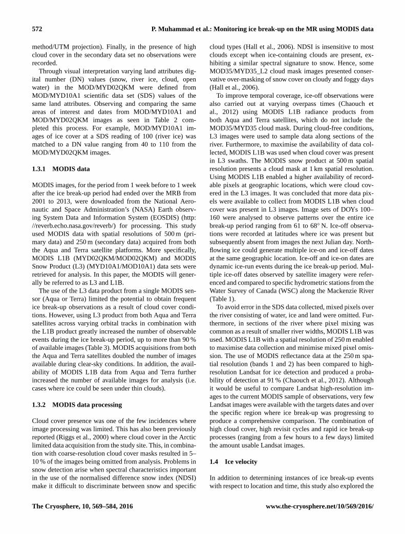
Table 1. Description of a water survey of Canada hydrometric stations on the Mackenzie River.
Station name Coordinates Distance downstream from mouth
of Mackenzie River (km)
Mackenzie River at Fort Providence 61.27◦ N, 117.54◦ W 75.8
Mackenzie River at Strong Point 61.81◦ N, 120.79◦ W 301
Mackenzie River at Fort Simpson 61.86◦ N, 121.35◦ W 330
Mackenzie River at Norman Wells 65.27◦ N, 126.84◦ W 890
Mackenzie River at Arctic Red River 67.45◦ N, 133.75◦ W 1435
Table 2. Scientific data set (SDS) and digital number (DN) values
from MODIS L1B and L3 products used for the Mackenzie River.
MOD/MYD MOD/MYD
L3 (SDS) L1B (DN)
Imag
eco
ver
Spatial resolution (500 m) (250 m)
Cloud cover 50 150<
Snow 200 111–150
Ice (snow covered) 100 40–110
Open water 37 30
Land 25 < 28
Wavelength
(nm)
Ban
ds
1 620–670
2 841–876
3 459–479
4 545–565
5 1230–1250
7 2105–2155
use of MODIS as a tool for estimating velocity of ice flows.
Ice velocity was observed and recorded on stretches of ice
debris (> 15 km) where ice and water demarcation was dis-
tinguishable. Stretches of ice were defined by the changes
in attributes on the Mackenzie River from open water to ice
(37–100) on the leading edge of ice and ice to open water
(100–37) on the trailing edge of ice. Velocity was estimated
by tracking the displacement of ice over time across multiple
MODIS L3 and L1B swaths. Displacement estimates over
time were made twice daily from Aqua and Terra satellites
image captures. It should be noted that the MODIS images
do not show displacement within each image capture; there-
fore the average velocities represent estimates between im-
ages. Average velocities were recorded until ice debris could
no longer be distinguished as a result of melt or cloud cover.
Ice velocities recorded also represent the lower limit of the
ice flows, as the ice may not be moving at all times between
image acquisitions. Therefore, the average velocities present
time periods when the ice could be at rest and, therefore, the
velocity measurements represent underestimation of the ac-
tual ice velocities. Ice debris movement was also referenced
Table 3. Time periods of observations and number of MODIS L3
and L1B images analysed during break-up on the Mackenzie River
(2001–2013).
Year Time period of MODIS L3 MODIS L1B
observations images images
(Julian day)
Aqua Terra Aqua Terra
2001 119–153 20 1 1
2002 136–150 13 2 1
2003 115–153 16 13 1 1
2004 122–151 9 6 3 2
2005 116–144 14 15 2 2
2006 123–144 12 15 1 1
2007 115–153 23 21 2 4
2008 124–154 18 23 2 4
2009 125–147 15 16 2 1
2010 115–141 17 18 1 1
2011 128–148 16 14 2 2
2012 123–149 20 16 1 2
2013 131–149 14 14 1 1
Total 174 204 21 23
to WSC station provided that an operational station was on
the route of the ice run.
1.5 Results
1.6 Thermal and dynamic ice break-up
Over the 13 years of analysis, the ice break-up period ranged
from as early as DOY 115 and lasted as late as DOY 155.
Most ice break-up over the 13-year period (2001–2013)
began between DOYs 115 and 125 and ended between
DOYs 145 and 155. River morphology acted as an important
spatial control determining the type of ice break-up process
and ice run. Ice break-up processes between years showed
different overall patterns with respect to location, and thus
temporally the beginning, end and duration of ice break-up
varied. For example, the initiation of ice break-up in 2002
(Fort Simpson, 330 km) began 10 days later than the average
date when ice would completely clear the river section. Com-
pared to 2007, the initiation of ice break-up began 13 days
www.the-cryosphere.net/10/569/2016/ The Cryosphere, 10, 569–584, 2016
574 P. Muhammad et al.: Monitoring ice break-up on the MR using MODIS data
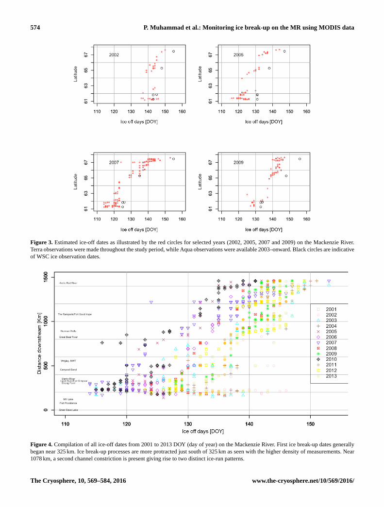
Figure 3. Estimated ice-off dates as illustrated by the red circles for selected years (2002, 2005, 2007 and 2009) on the Mackenzie River.
Terra observations were made throughout the study period, while Aqua observations were available 2003–onward. Black circles are indicative
of WSC ice observation dates.
Figure 4. Compilation of all ice-off dates from 2001 to 2013 DOY (day of year) on the Mackenzie River. First ice break-up dates generally
began near 325 km. Ice break-up processes are more protracted just south of 325 km as seen with the higher density of measurements. Near
1078 km, a second channel constriction is present giving rise to two distinct ice-run patterns.
The Cryosphere, 10, 569–584, 2016 www.the-cryosphere.net/10/569/2016/
P. Muhammad et al.: Monitoring ice break-up on the MR using MODIS data 575
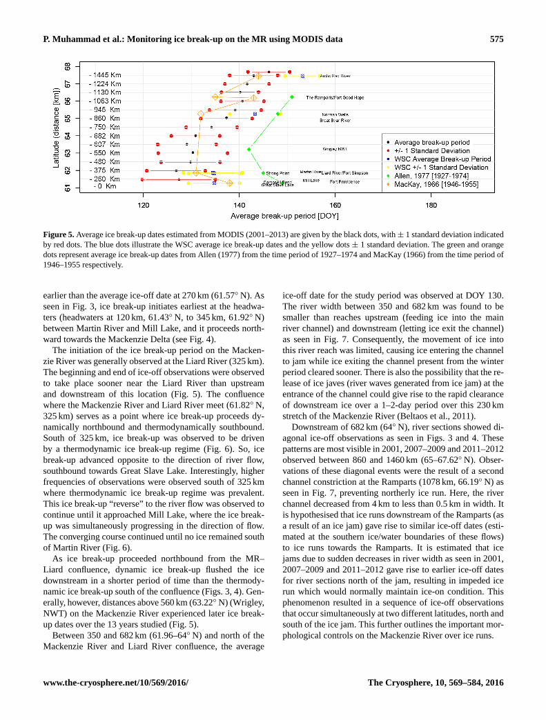
Figure 5. Average ice break-up dates estimated from MODIS (2001–2013) are given by the black dots, with ± 1 standard deviation indicated
by red dots. The blue dots illustrate the WSC average ice break-up dates and the yellow dots ± 1 standard deviation. The green and orange
dots represent average ice break-up dates from Allen (1977) from the time period of 1927–1974 and MacKay (1966) from the time period of
1946–1955 respectively.
earlier than the average ice-off date at 270 km (61.57◦ N). As
seen in Fig. 3, ice break-up initiates earliest at the headwa-
ters (headwaters at 120 km, 61.43◦ N, to 345 km, 61.92◦ N)
between Martin River and Mill Lake, and it proceeds north-
ward towards the Mackenzie Delta (see Fig. 4).
The initiation of the ice break-up period on the Macken-
zie River was generally observed at the Liard River (325 km).
The beginning and end of ice-off observations were observed
to take place sooner near the Liard River than upstream
and downstream of this location (Fig. 5). The confluence
where the Mackenzie River and Liard River meet (61.82◦ N,
325 km) serves as a point where ice break-up proceeds dy-
namically northbound and thermodynamically southbound.
South of 325 km, ice break-up was observed to be driven
by a thermodynamic ice break-up regime (Fig. 6). So, ice
break-up advanced opposite to the direction of river flow,
southbound towards Great Slave Lake. Interestingly, higher
frequencies of observations were observed south of 325 km
where thermodynamic ice break-up regime was prevalent.
This ice break-up “reverse” to the river flow was observed to
continue until it approached Mill Lake, where the ice break-
up was simultaneously progressing in the direction of flow.
The converging course continued until no ice remained south
of Martin River (Fig. 6).
As ice break-up proceeded northbound from the MR–
Liard confluence, dynamic ice break-up flushed the ice
downstream in a shorter period of time than the thermody-
namic ice break-up south of the confluence (Figs. 3, 4). Gen-
erally, however, distances above 560 km (63.22◦ N) (Wrigley,
NWT) on the Mackenzie River experienced later ice break-
up dates over the 13 years studied (Fig. 5).
Between 350 and 682 km (61.96–64◦ N) and north of the
Mackenzie River and Liard River confluence, the average
ice-off date for the study period was observed at DOY 130.
The river width between 350 and 682 km was found to be
smaller than reaches upstream (feeding ice into the main
river channel) and downstream (letting ice exit the channel)
as seen in Fig. 7. Consequently, the movement of ice into
this river reach was limited, causing ice entering the channel
to jam while ice exiting the channel present from the winter
period cleared sooner. There is also the possibility that the re-
lease of ice javes (river waves generated from ice jam) at the
entrance of the channel could give rise to the rapid clearance
of downstream ice over a 1–2-day period over this 230 km
stretch of the Mackenzie River (Beltaos et al., 2011).
Downstream of 682 km (64◦ N), river sections showed di-
agonal ice-off observations as seen in Figs. 3 and 4. These
patterns are most visible in 2001, 2007–2009 and 2011–2012
observed between 860 and 1460 km (65–67.62◦ N). Obser-
vations of these diagonal events were the result of a second
channel constriction at the Ramparts (1078 km, 66.19◦ N) as
seen in Fig. 7, preventing northerly ice run. Here, the river
channel decreased from 4 km to less than 0.5 km in width. It
is hypothesised that ice runs downstream of the Ramparts (as
a result of an ice jam) gave rise to similar ice-off dates (esti-
mated at the southern ice/water boundaries of these flows)
to ice runs towards the Ramparts. It is estimated that ice
jams due to sudden decreases in river width as seen in 2001,
2007–2009 and 2011–2012 gave rise to earlier ice-off dates
for river sections north of the jam, resulting in impeded ice
run which would normally maintain ice-on condition. This
phenomenon resulted in a sequence of ice-off observations
that occur simultaneously at two different latitudes, north and
south of the ice jam. This further outlines the important mor-
phological controls on the Mackenzie River over ice runs.
www.the-cryosphere.net/10/569/2016/ The Cryosphere, 10, 569–584, 2016

576 P. Muhammad et al.: Monitoring ice break-up on the MR using MODIS data
Figure 6. This example illustrates ice break-up at the headwaters of
the Mackenzie River system in 2005 from DOYs 120 to 125.
Based on MODIS imagery, ice break-up began on average
between DOYs 115 and 125 and ended between DOYs 145
and 155 (Fig. 5). The standard deviation of estimated ice-
off dates decreased with increasing latitude. MODIS-derived
dates showed highest deviations across river sections where
thermodynamic ice break-up was prevalent. These patterns
are similar to those seen from average break-up and stan-
dard deviations observed from the WSC. The 13-year aver-
age reveals similar ice conditions in the low, mid- and high
latitudes of the Mackenzie River from MODIS and WSC
data. There was an observed difference of 5 days between ice
break-up observed from MODIS imagery and WSC. Also,
the respective standard deviations overlap across the similar
periods. Ice break-up in general continued in a north to south
direction over the ice break-up periods. Near Forth Simpson
(330 km, 61.85◦ N), it is worth mentioning that ice break-up
was observed earlier than at more southern latitudes as il-
lustrated by MODIS observations. This pattern is likewise
visible from the WSC data.
1.7 Ice break-up and snowmelt
In order to assess the relative timing of ice disappearance
in relation to its surrounding sub-basin, the timing of river-
ice disappearance was qualitatively compared to the timing
of near complete snow disappearance from the surrounding
area. MODIS L3 imagery of different years was selected
which clearly revealed ice–snow relation with respect to lo-
cation, where cloud cover was a minimal issue.
Locations where thermodynamic ice disappearance was
hypothesised (south of 61.8◦ N, 325 km) corresponded with
patterns where ice disappeared much later than snow on
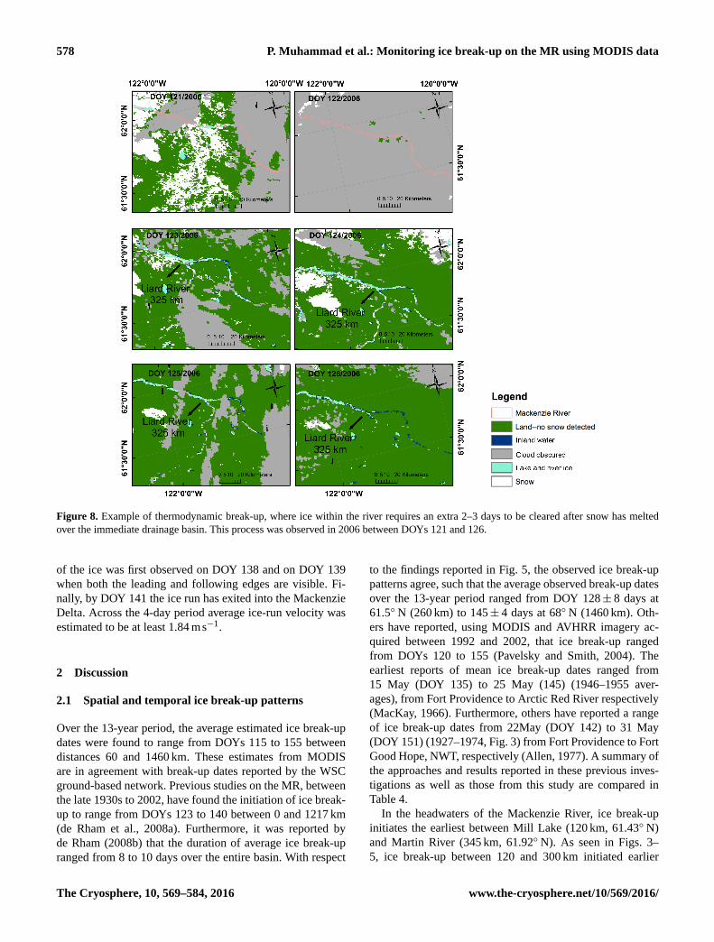
land (Fig. 6). For example, DOY 121/2006 (Fig. 8) was ob-
served to be the beginning of the snowmelt period at 290–
487 km (61.75–62.5◦ N) and this process ended when the
snow had almost completely disappeared by DOY 125. How-
ever, DOY 125 corresponded to the initiation of ice break-up.
This was not limited to 2006 so that snow generally disap-
peared sooner from surrounding sub-basins, followed by the
initiation of ice break-up.
At reaches north of the MR–Liard River confluence, ice
break-up and snowmelt were observed to initiate in sync
with one another. As seen in Fig. 9, on DOYs 136–137/2011,
ice disappearance on the southern cross-section of the fig-
ure is marked by the near simultaneous disappearance of
snow. In fact by DOY 140/2011 both ice and snow had
completely disappeared analogous to each other. On sec-
tions of the Mackenzie River before it enters the Macken-
zie Delta, estimated ice break-up and snow disappearance
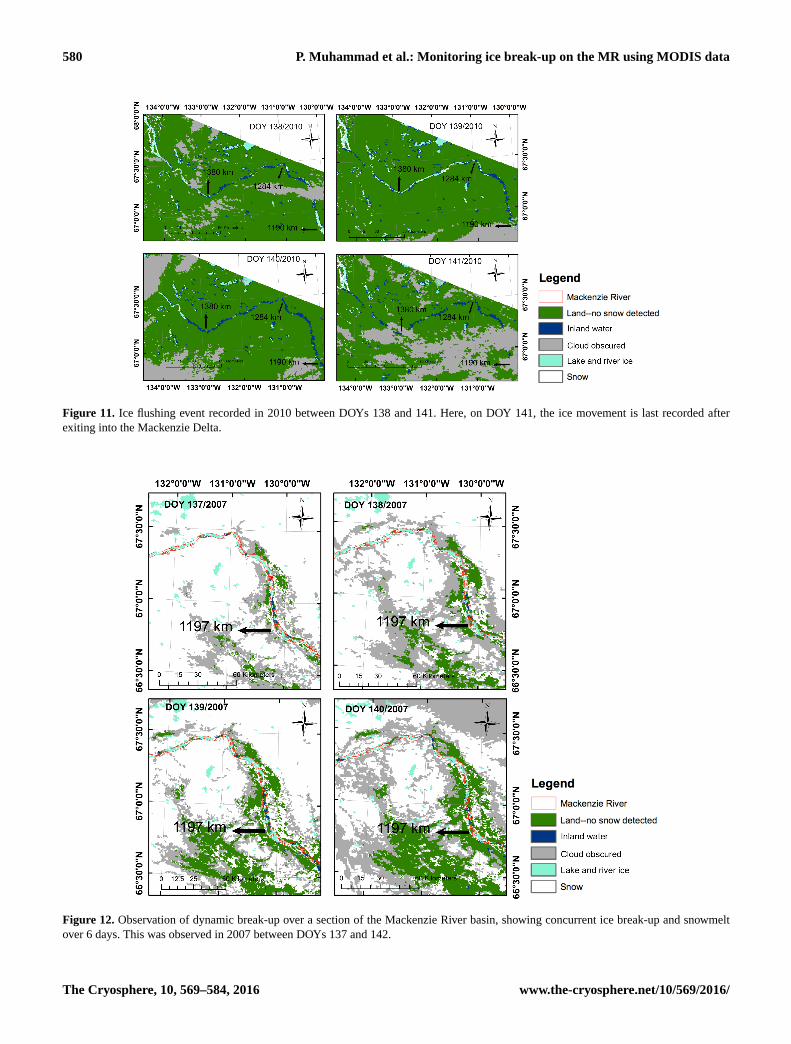
was again observed to occur almost simultaneously (Fig. 12).
Over a 6-day period (DOYs 137–142/2007) the ice break-
up process continued until ice completely disappeared from
the channel (MR). This process ensued sooner relative to
complete snowmelt over the surrounding sub-basins. By
DOY 142/2007 nearly one-third of the river was completely
The Cryosphere, 10, 569–584, 2016 www.the-cryosphere.net/10/569/2016/

P. Muhammad et al.: Monitoring ice break-up on the MR using MODIS data 577
Figure 7. Change in channel width along the Mackenzie River as observed in (a) (ca. 0–500 km), (b) (ca. 500–1000 km) and (c) (ca. 1000–
1500 km).
cleared of ice while most of the snow was still present over
the MRB.
Principally, it was concluded that on the upper Mackenzie
Basin snow cleared sooner than the initiation of ice break-up.
In the mid-Mackenzie Basin (375–860 km, 62–65◦ N), river
ice cleared in situ to snow clearance from the surrounding
basin. In fact, ice cleared sooner in the mid-basin than the up-
per Mackenzie Basin. Finally, in the lower Mackenzie Basin,
river ice cleared sooner than the snow from the surrounding
basin. This could be telling of a river continuum of the build-
up of mechanical strength used to clear river ice within the
Mackenzie River towards higher latitudes. The Liard River
tributary accounts for one-third of the total Mackenzie dis-
charge (Woo and Thorne, 2003), and so a rise in discharge in
May initiates earlier ice break-up downstream as a result of
increased stress induced on ice by a rise in river stage. Me-
chanical stress used to shove ice is continually magnified by
the addition of small and large tributaries downstream of the
Mackenzie River (Great Slave River, Arctic Red River).
1.8 River-ice velocity
Figures 10 and 11 illustrate ice movement from which ice ve-
locities could be estimated over periods of 3–4 days follow-
ing secondary channel constriction at 66◦ N. Here, ice runs
that contained over 15 km of entrained ice were chosen to es-
timate average ice velocities. Only periods with at least three
images with partial or no cloud cover were selected for ve-
locity estimates.
In 2008, the open-water/ice boundary (leading edge) was
recorded beginning on DOY 143 (Fig. 10). The open-
water/ice (northern edge of ice) and ice/open-water (fol-
lowing edge) boundaries were both visible from DOY 144.
Finally, the ice/open-water boundary was last observed on
DOY 145. The average ice-run velocity between 1063 and
1210 km (66–66.95◦ N) over the 3 days was estimated to
be at least 1.21 ms−1. Likewise, in 2010 (Fig. 11), open-
water/ice (leading end) and ice/open-water (following end)
was observed between DOYs 138 and 141. The leading edge
www.the-cryosphere.net/10/569/2016/ The Cryosphere, 10, 569–584, 2016
578 P. Muhammad et al.: Monitoring ice break-up on the MR using MODIS data
Figure 8. Example of thermodynamic break-up, where ice within the river requires an extra 2–3 days to be cleared after snow has melted
over the immediate drainage basin. This process was observed in 2006 between DOYs 121 and 126.
of the ice was first observed on DOY 138 and on DOY 139
when both the leading and following edges are visible. Fi-
nally, by DOY 141 the ice run has exited into the Mackenzie
Delta. Across the 4-day period average ice-run velocity was
estimated to be at least 1.84 ms−1.
2 Discussion
2.1 Spatial and temporal ice break-up patterns
Over the 13-year period, the average estimated ice break-up
dates were found to range from DOYs 115 to 155 between
distances 60 and 1460 km. These estimates from MODIS
are in agreement with break-up dates reported by the WSC
ground-based network. Previous studies on the MR, between
the late 1930s to 2002, have found the initiation of ice break-
up to range from DOYs 123 to 140 between 0 and 1217 km
(de Rham et al., 2008a). Furthermore, it was reported by
de Rham (2008b) that the duration of average ice break-up
ranged from 8 to 10 days over the entire basin. With respect
to the findings reported in Fig. 5, the observed ice break-up
patterns agree, such that the average observed break-up dates
over the 13-year period ranged from DOY 128 ± 8 days at
61.5◦ N (260 km) to 145 ± 4 days at 68◦ N (1460 km). Oth-
ers have reported, using MODIS and AVHRR imagery ac-
quired between 1992 and 2002, that ice break-up ranged
from DOYs 120 to 155 (Pavelsky and Smith, 2004). The
earliest reports of mean ice break-up dates ranged from
15 May (DOY 135) to 25 May (145) (1946–1955 aver-
ages), from Fort Providence to Arctic Red River respectively
(MacKay, 1966). Furthermore, others have reported a range
of ice break-up dates from 22May (DOY 142) to 31 May
(DOY 151) (1927–1974, Fig. 3) from Fort Providence to Fort
Good Hope, NWT, respectively (Allen, 1977). A summary of
the approaches and results reported in these previous inves-
tigations as well as those from this study are compared in
Table 4.
In the headwaters of the Mackenzie River, ice break-up
initiates the earliest between Mill Lake (120 km, 61.43◦ N)
and Martin River (345 km, 61.92◦ N). As seen in Figs. 3–
5, ice break-up between 120 and 300 km initiated earlier
The Cryosphere, 10, 569–584, 2016 www.the-cryosphere.net/10/569/2016/

P. Muhammad et al.: Monitoring ice break-up on the MR using MODIS data 579
Figure 9. Snowmelt and ice run over the Mackenzie River basin in 2011 between the DOYs 137 and 140. There is a 2-day lag between the
complete clearance of snow on land and the clearance of ice on the Mackenzie River.
Figure 10. Ice flushing event recorded in 2008 between DOYs 143 and 146.
www.the-cryosphere.net/10/569/2016/ The Cryosphere, 10, 569–584, 2016
580 P. Muhammad et al.: Monitoring ice break-up on the MR using MODIS data
Figure 11. Ice flushing event recorded in 2010 between DOYs 138 and 141. Here, on DOY 141, the ice movement is last recorded after
exiting into the Mackenzie Delta.
Figure 12. Observation of dynamic break-up over a section of the Mackenzie River basin, showing concurrent ice break-up and snowmelt
over 6 days. This was observed in 2007 between DOYs 137 and 142.
The Cryosphere, 10, 569–584, 2016 www.the-cryosphere.net/10/569/2016/
P. Muhammad et al.: Monitoring ice break-up on the MR using MODIS data 581
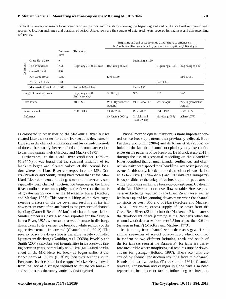
Table 4. Summary of results from previous investigations and this study showing the beginning and end of the ice break-up period with
respect to location and range and duration of period. Also shown are the sources of data used, years covered for analyses and corresponding
references.
Beginning and end of ice break-up dates relative to distance on
the Mackenzie River as reported by previous investigations (Julian days)
Distances This study
(km)
Loca
tions
Great Slave Lake 0 Beginning at 120
Fort Providence 75.8 Beginning at 128±8 days Beginning at 123 Beginning at 135 Beginning at 142
Camsell Bend 456
Fort Good Hope 1080 End at 140 End at 151
Arctic Red River 1437 End at 145
Mackenzie River End 1460 End at 145±4 days End at 155
Range of break-up dates Beginning at ±8 8–10 days N/A N/A N/A
End at ±4 days
Data source MODIS WSC Hydrometric MODIS/AVHRR Ice Surveys WSC Hydrometric
stations Stations
Years covered 2001–2013 1930s–2002 1992–2002 1946–1955 1927–1974
Reference de Rham ( 2008b) Pavelsky and MacKay (1966) Allen (1977)
Smith (2004)
as compared to other sites on the Mackenzie River, but ice
cleared later than other for other river sections downstream.
Here ice in the channel remains stagnant for extended periods
of time as ice usually freezes to bed and is most susceptible
to thermodynamic melt (MacKay and Mackay, 1973).
Furthermore, at the Liard River confluence (325 km,
61.84◦ N) it was found that the seasonal initiation of ice
break-up began and cleared earliest at this central loca-
tion where the Liard River converges into the MR. Oth-
ers (Pavelsky and Smith, 2004) have noted that at the MR–
Liard River confluence flooding is common between years,
especially near channel junction. Ice break-up at the Liard
River confluence occurs rapidly, as the flow contribution is
of greater magnitude than the Mackenzie River (MacKay
and Mackay, 1973). This causes a lifting of the river stage,
exerting pressure on the ice cover and resulting in ice jam
downstream most often attributed to the presence of channel
bending (Camsell Bend, 456 km) and channel constriction.
Similar processes have also been reported for the Susque-
hanna River, USA, where an observed increase in discharge
downstream fosters earlier ice break-up while sections of the
upper river remain ice covered (Chaouch et al., 2012). The
severity of ice break-up stage is therefore largely controlled
by upstream discharge (Goulding et al., 2009b). Pavelsky and
Smith (2004) also observed irregularities in ice break-up tim-
ing between years, particularly at 325 km (MR–Liard conflu-
ence) on the MR. Here, ice break-up began earlier at dis-
tances north of 325 km (61.8◦ N) than river sections south.
Postponed ice break-up in the upper Mackenzie can result
from the lack of discharge required to initiate ice break-up
and so the ice is thermodynamically disintegrated.
Channel morphology is, therefore, a more important con-
trol on ice break-up patterns than previously believed. Both
Pavelsky and Smith (2004) and de Rham et al. (2008a) al-
luded to the fact that channel morphology may exert influ-
ences on the patterns of ice break-up. De Munck et al. (2011),
through the use of geospatial modelling on the Chaudière
River identified that channel islands, confluences and chan-
nel sinuosity predisposed the Chaudière River to ice jamming
events. In this study, it is determined that channel constriction
at 350–682 km (61.96–64◦ N) and 1078 km (the Ramparts)
is responsible for the delay of ice break-up timings upstream
while promoting earlier ice break-up downstream. Upstream
of the Liard River junction, river flow is stable. However, ex-
cessive discharge supplied by the Liard River causes earlier
ice break-up and ice jamming downstream when the channel
constricts between 350 and 682 km (MacKay and Mackay,
1973). Furthermore, excess supply of ice cover from the
Great Bear River (821 km) into the Mackenzie River causes
the development of ice jamming at the Ramparts when the
channel width decreases from over 3.5 km to less than 0.6 km
(as seen in Fig. 7) (MacKay and Mackay, 1973).
Ice jamming from channel width decreases gave rise to
similar sequences of ice-off observations, which occurred
in tandem at two different latitudes, north and south of
the ice jam (as seen at the Ramparts). Ice jams are there-
fore favourable where morphological features impede down-
stream ice passage (Beltaos, 1997). These ice jams are
caused by channel constriction resulting from mid-channel
islands and narrow reaches (Terroux et al., 1981). Channel
braiding, constriction and changes in slope have also been
reported to be important factors influencing ice break-up
www.the-cryosphere.net/10/569/2016/ The Cryosphere, 10, 569–584, 2016
582 P. Muhammad et al.: Monitoring ice break-up on the MR using MODIS data
and flow regimes (de Rham et al., 2008a). In the context of
our study, it was found that channel constrictions and bends
represented locations where ice runs were impeded. Hicks
(2009) also reported that running ice may be stalled when ge-
ometric constraints such as tight bends, narrow sections and
islands are present in rivers. In fact, it has been shown that
ice debris flow drop to a velocity of 0 in the presence of flow
depths near channels islands and bars (Kääb et al., 2013).
Lastly, Kääb and Prowse (2011), using ALOS PRISM stereo
imagery on the Mackenzie River determined that ice veloci-
ties decrease to 0 in the presence of bars.
The estimated ice-run events illustrated in Figs. 7 and 10
may have been caused by ice jam releases (javes) initiated at
the Ramparts (1078 km, 66.19◦ N). Such processes may also
be the reason why ice was estimated to be cleared at higher
latitudes before the end of the snowmelt period. Accumulated
stress with the rise of water levels behind the jam can result
in sufficient kinetic energy to clear river ice downstream be-
fore the complete snowmelt overlying the surrounding sub-
basins.
2.2 Ice velocities
Ice-run velocities are believed to be the highest where
the ice is minimally effected by channel morphology, un-
connected from incoming tributaries, and channel splitting
which causes the formation of islands (Kääb et al., 2013).
Amongst the variety of ice runs observed over 13 years,
ice velocities could be quantified in 2008 and 2010. Over
3–4-day periods, average ice velocities were estimated to
be 1.21 ms−1 (2008) and 1.84 ms−1 (2010). More impor-
tantly, it is believed that the evolution of such velocities is
the product of javes. Our measurements of ice-run veloc-
ity in 2008 coincidently synchronise with other indepen-
dent satellite- and ground-based ice measurements. Exten-
sive measurements of ice runs in 2008 around MR–Arctic
Red River junction are believed to be generated by waves
released from released ice jams (Beltaos, 2013). This aligns
with ice jams which may form at the Ramparts (1078 km,
66.19◦ N) as a result of channel constriction. The evolu-
tion of ice runs north of the Ramparts (flowing past the
Arctic Red River) observed over DOYs 143–146/2008 (22–
25 May/1.21 ms−1) matches similar ground measurements
(1.7 ms−1) made by Beltaos et al. (2012). Across the same
cross-section of the MR, Kääb and Prowse (with imagery
acquired 1–2 days earlier in 2008) estimated a preceding
ice run ranging from 0 to 3.2 ms−1. The highest flow ve-
locities were outlined where ice debris flow was most con-
centrated on the outside turn of the river bend. Finally, in
another independent study, Beltaos and Kääb (2014) found
ice debris velocities to range between 1 and 2 ms−1 using
ALOS PRISM imagery in 2010. Again these high-resolution
(2.5 m) image measurements compare quite well with our es-
timates from relatively coarse spatial resolution (250–500 m)
MODIS imagery. Additionally, early investigations have re-
ported that ice can clear at velocities of 0.27 and 0.44 ms−1
at Fort Simpson and Fort Good Hope respectively during the
ice break-up season (Terroux et al., 1981).
MODIS is shown to be a viable tool for estimating river-
ice velocities. This study finds that in order to monitor ice
cover the river width needs to at least 0.5–1 km wide. Fur-
thermore, to quantify river-ice velocities, the river width
needs to be at least 1 km wide. With respect to the MR, ice
velocities were only quantifiable above the Ramparts. The
presence of morphological controls and therefore river width
shortening leading to impeded ice run prevented quantifying
velocities, as leading river-ice demarcations were difficult to
locate. However, it was possible to estimate the overall veloc-
ity by observing ice/open-water boundaries. Lastly, it was de-
termined that in order to measure ice-run velocities without
major disturbance with impeded flows with respect to river
morphology, estimates with MODIS should be made north
of the Ramparts. North of the Ramparts, river widths were
generally observed to be largest with respect to other parts of
the MR.
3 Conclusion
The aim of this study was to develop an approach to estimate
ice break-up dates on the Mackenzie River over more than
a decade using MODIS snow and radiance products. It was
found that the initiation of ice break-up started on average
DOYs 115–125 and ended DOYs 145–155 over the 13 years
analysed. Thermal ice break-up was an important process
driving ice break-up south of the Liard River. Conversely,
north of the Liard, ice break-up was dynamically driven. The
addition to discharge from the MR–Liard River confluence
outlined a location where initial ice break-up began. Fur-
thermore, MODIS images allowed for the identification of
important factors controlling ice runs and ice break-up, in-
cluding morphological controls such as channel bars, river
meandering and channel constriction.
MODIS is currently the most promising tool for fre-
quent monitoring of river-ice processes as ground-based sta-
tions along the Mackenzie River are continuously being
closed. Operating aboard two satellites (Aqua and Terra), the
MODIS sensor allows for multiple daily acquisitions simul-
taneously along extensive stretches of the MR. Furthermore,
MODIS is proving to be a viable sensor for the monitoring of
river ice as shown in this and other recent investigations (e.g.
Chaouch et al., 2012). In this study, monitoring of ice break-
up on the Mackenzie River with MODIS proved to be a ro-
bust approach when compared to WSC ground-based obser-
vations. MODIS observations also allowed for the analysis
of basin level processes influencing ice break-up, including
river morphology and snowmelt.
Finally, future research should focus on investigating river-
ice processes using a combination of ground-based and
satellite-based sensors, particularly for examining relations
The Cryosphere, 10, 569–584, 2016 www.the-cryosphere.net/10/569/2016/

P. Muhammad et al.: Monitoring ice break-up on the MR using MODIS data 583
between river morphology, ice strength and discharge. Data
from these complementary technologies would be valuable
in the context of an early warning system for municipalities
where river-ice break-up is an important spring event caus-
ing significant flood damage. Furthermore, a multi-sensor ap-
proach using both optical and synthetic aperture radar (SAR)
data would be advantageous in order to monitor ice river pro-
cesses and floods in near real time. Satellite data from recent
and upcoming SAR (Sentinel-1 and RADARSAT Constel-
lation) and optical (Sentinel-2 and Sentinel-3) satellite mis-
sions will make such monitoring possible in the near future.
Acknowledgements. This research was supported by a NSERC
Discovery grant number 193583-2012 to C. Duguay. We are grate-
ful for the helpful comments of Ross Brown and two anonymous
reviewers.
Edited by: R. Brown
References
Abdul Aziz, O. I. and Burn, D. H.: Trends and variability in the
hydrological regime of the Mackenzie River Basin, J. Hydrol.,
319, 282–294, doi:10.1016/j.jhydrol.2005.06.039, 2006.
Allen, W. T. R.: Freeze-up, Break-up and Ice Thickness in Canada:
Embâcle, Débâcle Et Épaisseur de la Glace Au Canada, Environ-
nement Atmosphérique, Downsview, Ontario, USA, 1977.
Beltaos, S.: Onset of river ice breakup, Cold Reg. Sci. Technol., 25,
183–196, doi:10.1016/S0165-232X(96)00011-0, 1997.
Beltaos, S.: Progress in the study and management of river ice jams,
Cold Reg. Sci. Technol., 51, 2–19, 2008.
Beltaos, S.: Hydrodynamic characteristics and effects of river waves
caused by ice jam releases, Cold Reg. Sci. Technol., 85, 42–55,
doi:10.1016/j.coldregions.2012.08.003, 2013.
Beltaos, S. and Carter, T.: Field studies of ice breakup and jamming
in lower Peace River, Canada, Cold Reg. Sci. Technol., 56, 102–
114, doi:10.1016/j.coldregions.2008.11.002, 2009.
Beltaos, S. and Kääb, A.: Estimating river discharge during ice
breakup from near-simultaneous satellite imagery, Cold Reg. Sci.
Technol., 98, 35–46, 2014.
Beltaos, S. and Prowse, T.: River-ice hydrology in
a shrinking cryosphere, Hydrol. Process., 23, 122–144,
doi:10.1002/hyp.7165, 2009.
Beltaos, S., Rowsell, R., and Tang, P.: Remote data collection on ice
breakup dynamics: Saint John River case study, Cold Reg. Sci.
Technol., 67, 135–145, doi:10.1016/j.coldregions.2011.03.005,
2011.
Beltaos, S., Carter, T., and Rowsell, R.: Measurements and analy-
sis of ice breakup and jamming characteristics in the Mackenzie
Delta, Canada, Cold Reg. Sci. Technol., 82, 110–123, 2012.
Chaouch, N., Temimi, M., Romanov, P., Cabrera, R., McKillop, G.,
and Khanbilvardi, R.: An automated algorithm for river ice mon-
itoring over the Susquehanna River using the MODIS data, Hy-
drol. Process., 28, 62–73, doi:10.1002/hyp.9548, 2012.
Dee, D. P., Uppala, S. M., Simmons, A. J., Berrisford, P., Poli,
P., Kobayashi, S., Andrae, U., Balmaseda, M. A., Balsamo, G.,
Bauer, P., Bechtold, P., Beljaars, A. C. M., van de Berg, L., Bid-
lot, J., Bormann, N., Delsol, C., Dragani, R., Fuentes, M., Geer,
A. J., Haimberger, L., Healy, S. B., Hersbach, H., Hólm, E. V.,
Isaksen, L., Kållberg, P., Köhler, M., Matricardi, M., McNally,
A. P., Monge-Sanz, B. M., Morcrette, J.-J., Park, B.-K., Peubey,
C., de Rosnay, P., Tavolato, C., Thépaut, J.-N., and Vitart, F.: The
ERA-Interim reanalysis: configuration and performance of the
data assimilation system, Q. J. Roy. Meteor. Soc., 137, 553–597,
doi:10.1002/qj.828, 2011.
De Munck, S., Gauthier, Y., Bernier, M., Poulin, J., and Chokmani,
K.: Preliminary development of a geospatial model to estimate
a river channel’s predisposition to ice jams, in: 16th Workshop
on Hydraulics of Ice Covered Rivers, Winnipeg, Manitoba, 18–
22 September 2011, CGU HS Committee on River Ice Processes
and the Environment (CRIPE), 2011.
de Rham, L. P., Prowse, T. D., Beltaos, S., and Lacroix, M. P.:
Assessment of annual high-water events for the Macken-
zie River basin, Canada, Hydrol. Process., 22, 3864–3880,
doi:10.1002/hyp.7016, 2008a.
de Rham, L. P., Prowse, T. D., and Bonsal, B. R.: Tem-
poral variations in river-ice break-up over the Macken-
zie River Basin, Canada, J. Hydrol., 349, 441–454,
doi:10.1016/j.jhydrol.2007.11.018, 2008b.
Goulding, H. L., Prowse, T. D., and Beltaos, S.: Spatial and
temporal patterns of break-up and ice-jam flooding in the
Mackenzie Delta, NWT, Hydrol. Process., 23, 2654–2670,
doi:10.1002/hyp.7251, 2009a.
Goulding, H. L., Prowse, T. D., and Bonsal, B.: Hydroclimatic
controls on the occurrence of break-up and ice-jam flooding in
the Mackenzie Delta, NWT, Canada, J. Hydrol., 379, 251–267,
doi:10.1016/j.jhydrol.2009.10.006, 2009b.
Government of Canada, E. C.: Environment Canada – Water –
Rivers, available at: http://www.ec.gc.ca/eau-water/default.asp?
lang=En&n=45BBB7B8-1, last access: 7 June 2014, 2007.
Government of Canada, E. C.: Environment Canada – Water –
Environment Canada Data Explorer, available at: http://www.
ec.gc.ca/rhc-wsc/default.asp?lang=En&n=0A47D72F-1, last ac-
cess: 27 March 2013, 2010.
Hall, D. D. K., Riggs, D. G. A., and Salomonson, D. V. V.: MODIS
snow and sea ice products, in: Earth Science Satellite Remote
Sensing, edited by: Qu, P. J. J., Gao, D. W., Kafatos, P. M., Mur-
phy, D. R. E., and Salomonson, D. V. V., Springer, Berlin, Hei-
delberg, 154–181, 2006.
Hicks, F.: An overview of river ice problems: CRIPE07 guest edito-
rial, Cold Reg. Sci. Technol., 55, 175–185, 2009.
Kääb, A. and Prowse, T.: Cold-regions river flow ob-
served from space, Geophys. Res. Lett., 38, L08403,
doi:10.1029/2011GL047022, 2011.
Kääb, A., Lamare, M., and Abrams, M.: River ice flux and wa-
ter velocities along a 600 km-long reach of Lena River, Siberia,
from satellite stereo, Hydrol. Earth Syst. Sci., 17, 4671–4683,
doi:10.5194/hess-17-4671-2013, 2013.
Lenormand, F., Duguay, C. R., and Gauthier, R.: Development
of a historical ice database for the study of climate change in
Canada, Hydrol. Process., 16, 3707–3722, 2002.
MacKay, D. K.: Mackenzie River and Delta ice survey, 1965, Geogr.
Bull., 8, 270–278, 1966.
MacKay, D. K. and Mackay, J. R.: Locations of Spring Ice Jamming
on the Mackenzie River, N. W. T. Environ.-Soc. Com. North.
www.the-cryosphere.net/10/569/2016/ The Cryosphere, 10, 569–584, 2016

584 P. Muhammad et al.: Monitoring ice break-up on the MR using MODIS data
Pipelines Task Force North. Oil Dev. Rep. No. 73-3 Technical
Report 8, North Pipelines Task Force North, Ottawa, 1973.
Magnuson, J. J., Robertson, D. M., Benson, B. J., Wynne, R. H.,
Livingstone, D. M., Arai, T., Assel, R. A., Barry, R. G., Card,
V., Kuusisto, E., Granin, N. G., Prowse, T. D., Stewart, K. M.,
and Vuglinski, V. S.: Historical trends in lake and river Ice
cover in the Northern Hemisphere, Science, 289, 1743–1746,
doi:10.1126/science.289.5485.1743, 2000.
Pavelsky, T. M. and Smith, L. C.: Spatial and temporal pat-
terns in Arctic river ice breakup observed with MODIS and
AVHRR time series, Remote Sens. Environ., 93, 328–338,
doi:10.1016/j.rse.2004.07.018, 2004.
Prowse, T. D.: River-ice ecology. I: Hydrologic, geomorphic,
and water-quality aspects, J. Cold Reg. Eng., 15, 1–16,
doi:10.1061/(ASCE)0887-381X(2001)15:1(1), 2001.
Prowse, T. D. and Beltaos, S.: Climatic control of river-
ice hydrology: a review, Hydrol. Process., 16, 805–822,
doi:10.1002/hyp.369, 2002.
Riggs, G. A., Barton, J. S., Casey, K. A., Hall, D. K., and Salomon-
son, V. V.: MODIS Snow Products Users’ Guide, NASA GSFC,
Greenbelt, MD, USA, 2000.
Terroux, A. C. D., Sherstone, D. A., Kent, T. D., Anderson, J. C.,
Bigras, S. C., and Kriwoken, L. A.: Ice regime of the lower
Mackenzie River and Mackenzie Delta, Environ. Can. Natl. Hy-
drol. Res. Inst., Hull, Quebec, 1981.
Woo, M.-K. and Thorne, R.: Streamflow in the Mackenzie Basin,
Canada, Arctic, 56, 328–340, 2003.
The Cryosphere, 10, 569–584, 2016 www.the-cryosphere.net/10/569/2016/