1

To be presented at the ASHRAE 2006 Summer Meeting, Quebec City, Canada, June 24-28, 2006, and published in ASHRAE Transactions. LBNL-58912.

Monitored Energy Performance of Electrochromic Windows Controlled for Daylight and Visual Comfort Eleanor S. Lee*, Dennis L. DiBartolomeo, Joseph H. Klems, Mehry

Yazdanian, Stephen E. Selkowitz Building Technologies Program, Environmental Energy Technologies Division, Lawrence Berkeley

National Laboratory, Mailstop 90-3111, 1 Cyclotron Road, Berkeley, CA 94720, USA Abstract

A 20-month field study was conducted to measure the energy performance of south-facing large-area

tungsten-oxide absorptive electrochromic (EC) windows with a broad switching range in a private office setting. The EC windows were controlled by a variety of means to bring in daylight while minimizing window glare. For some cases, a Venetian blind was coupled with the EC window to block direct sun. Some tests also involved dividing the EC window wall into zones where the upper EC zone was controlled to admit daylight while the lower zone was controlled to prevent glare yet permit view. If visual comfort requirements are addressed by EC control and Venetian blinds, a 2-zone EC window configuration provided average daily lighting energy savings of 10±15% compared to the reference case with fully lowered Venetian blinds. Cooling load reductions were 0±3%. If the reference case assumes no daylighting controls, lighting energy savings would be 44±11%. Peak demand reductions due to window cooling load, given a critical demand-response mode, were 19-26% maximum on clear sunny days. Peak demand reductions in lighting energy use were 0% or 72-100% compared to a reference case with and without daylighting controls, respectively. Lighting energy use was found to be very sensitive to how glare and sun is controlled. Additional research should be conducted to fine-tune EC control for visual comfort based on solar conditions so as to increase lighting energy savings.

Keywords: Building envelope, building automation and controls, commercial buildings

1. Introduction

Past simulation studies have indicated that electrochromic façade systems have the technical potential to significantly reduce energy use and peak demand in residential and nonresidential buildings. Electrochromic windows can vary their tint reversibly with the application of a small applied dc voltage (gasochromic are of the same basic composition but switch with the insertion of an inert gas into the between-pane gap of an insulating glass unit (IGU)). Some of these studies (primarily conducted in the 1980s to early 1990s) estimated that EC windows with daylighting controls can reduce annual energy use by 20-30% in commercial office buildings situated in moderate to hot climates if the EC window is controlled to manage daylight compared to conventional windows with daylighting controls (e.g., Sullivan et al. 1994). Simulation studies have also been conducted to identify control algorithms that best minimize energy use in various climates (Karlsson 2001, Gugliermetti and Bisegna 2003). These studies spurred early R&D investment in this new emerging technology with the hopes that deployment of such technologies would significantly improve the energy efficiency of future building stock. * Contact: E.S. Lee, Lawrence Berkeley National Laboratory, Mailstop 90-3111, 1 Cyclotron Road, Berkeley, CA 94720, (510) 486-4997, (510) 486-4089 fax, eslee@lbl.gov.

2

As the material science R&D on chromogenic coatings matured, moving from the laboratory producing small-area (0.075 m, 0.25 ft square) samples to pilot production facilities producing large-area (1-2 m2, 11-22 ft2) windows in the late 1990s, the focus of the applications side of R&D shifted from simulations to full-scale testing of pre-market devices in real-world applications in order to identify and address unforeseen engineering issues, gauge user acceptance, and measure actual energy-savings under realistic weather conditions. This activity has been particularly important for the electrochromic technology because accurate solar-optical characterization of this glazing material has been challenging. Simulation tools do not yet adequately describe the various control systems and response characteristics of the technologies involved. Furthermore, automating control of switchable windows with other building control systems to achieve energy efficient and comfortable conditions is yet unproven and presents very relevant challenges.

To date, several field studies have been conducted over the past few years employing large-area electrochromic windows that were deemed sufficiently mature for market introduction. “Maturity” was defined by devices that had acceptable appearance (e.g., uniformity of tint), good potential durability, and the potential to be manufactured at low cost. In 1999, a four-month study was conducted by the Lawrence Berkeley National Laboratory (LBNL) in two private offices involving continuously modulated large-area EC windows integrated with daylighting controls (Lee and DiBartolomeo 2002). The study mapped basic characteristics of EC windows (switching range, switching speed) to monitored performance variables and presented lighting energy use savings and visual comfort data for daylight- and glare-controlled EC windows. No thermal data were monitored and the length of the study was short, providing limited information on annual performance. Within the three-year EU Switchable Facade Technology (SWIFT) program (completed in 2003), several field studies were undertaken, one for a residential application and several for typical private offices that are common to commercial buildings (Platzer 2003). These studies were undertaken to gain real-world experience with electrochromic (the same type used for the 1999 LBNL study) and gasochromic facades, evaluate user reactions to switchable facades, and monitor various environmental variables interior air and operative temperatures, illuminance, luminance distributions over a 2-week period) compared to conventional windows. These field studies were limited and did not provide sufficient monitored data to confirm year-round energy use savings and comfort.

In these prior field studies, the tungsten-oxide-based (WO3) absorptive electrochromic and gasochromic windows tested did not possess a broad switching range: i.e., the center-of-glass visible transmittance (Tv) range was Tv=0.50-15. Earlier simulations studies identified a key drawback: tinted glass cannot block direct sun. This poses two problems: (1) occupants will experience glare discomfort if the orb of the sun is within view – unless the glass tint is almost opaque (Tv< 0.001) and (2) if the entire window is switched to control this direct source glare, interior daylight and lighting energy savings will be significantly reduced. The material science community has since responded by developing near-instant switchable reflective chromogenic materials that not only provide more efficient heat gain rejection but can also block direct sun by switching to a completely mirrored state. For the near-term absorptive electrochromic windows, prior energy simulation studies are likely to have provided overestimates of its energy-savings potential because the simulations were conducted with the EC window controlled for daylight optimization and not direct sun control and glare. The most relevant question of today is: “by how much?”

Several studies have been conducted since to ameliorate this situation. Under the SWIFT program, Fraunhofer Institute for Solar Energy Systems (ISE) conducted a user assessment study in two private offices with gasochromic windows installed (Wienold 2003). Twenty-seven subjects (23-35 years old) were asked to do reading, typing and letter search tasks involving a flat-screen visual display terminal (VDT). The tests conditions subjected occupants only to indirect glare (diffuse sky or indirect sunlight) within their peripheral view. Subjects rated the discomfort glare resulting from the bleached state (Tv=0.60) as “just acceptable” glare while the colored state (Tv=0.16) was rated better with “just perceptible” glare. For this view, the maximum acceptable average window luminance was found to be 5000 cd/m2. These tests established that the EC transmittance range was adequate for controlling indirect glare. U.S. climates tend to be much sunnier than the northern European climates, so these results, while relevant, advanced us one step closer towards answering the above question.

Wienold then went on to conduct a Radiance-ESP-r simulation study to estimate lighting and cooling energy use savings for electrochromic and gasochromic systems combined with a Venetian blind where the windows were controlled to block solar radiation during the summer and admit it during the winter, while the Venetian blind was modeled to emulate “manual” control – the blind was lowered and the slat angle

3

was tilted to block direct sun incident on the occupant’s eye and desk surface and to maintain the window luminance level below 5000 cd/m2. Energy savings were found to be highly dependent (factors of 2-4) on the maximum acceptable window luminance threshold. And this threshold unfortunately varies amongst various standards, occupant views, and applications: e.g., 400 cd/m2 for old cathode ray tube computer monitors versus 4000-5000 cd/m2 for the modern day flat-screen low-reflectance monitors.

This field study comes to the same basic conclusion as Wienold’s simulation study using control strategies tailored for the U.S. climate and based on field data using actual EC windows and daylighting control systems: energy savings are highly dependent on how the façade system manages visual discomfort. This study presents the measured energy performance resulting from various control algorithms and façade configurations designed to mitigate direct sun and glare while providing daylight. It relies on user assessment work conducted in the same field test facility. The WO3-based absorptive electrochromic (EC) windows tested were market-ready prototypes coupled with an immature “alpha” window controller designed to switch the EC windows to intermediate states. These EC windows have a broader switching range than those tested in previous field studies (Tv=0.60-0.05, center-of-glass solar heat gain coefficient (SHGC)=0.42-0.09). Fifteen EC windows have been controlled in each of two test rooms and their control has been integrated with a dimmable daylighting control system. Daily lighting energy use, cooling loads, and peak cooling loads were monitored over a 20-month period in a moderate sunny climate.

Figure 1. Floor plan (left) and cross-section (right) of test facility.

2. Method

2.1. Facility Description

A new 88.4 m2 (952 ft2) window systems testbed facility was built at LBNL, Berkeley, California (latitude 37°4'N, longitude 122°1'W) in Summer 2003. The facility was designed to evaluate the difference in thermal, daylighting, and control system performance between various façade, lighting, and some mechanical systems, as well as to conduct human factor studies under realistic weather conditions. The facility consists of three identical side-by-side test rooms built with nearly identical building materials to imitate a commercial office environment (Figure 1).

Each test room is 3.05 m wide by 4.57 m deep by 3.35 m high (10x15x11 ft) and has a 3.05 m wide by 3.35 m tall (10x11 ft) reconfigurable window wall facing due south. The windows in each test room are simultaneously exposed to approximately the same interior and exterior environment so that measurements between the three rooms can be compared. Direct sun is minimally obstructed by exterior obstructions: the altitude of exterior obstructions is less than 20° for azimuth angles between 90-140° (0°=north) and less

4

than 8° for azimuth angles between 240-270°. Interior surface reflectances of the floor, walls, and ceiling, are 0.18, 0.85, and 0.86, respectively, as measured by a Minolta CM-2002 spectroreflectometer. Interior furnishings include an L-shaped desk, flat-screen LCD monitor, and two chairs. The rooms were designated as Rooms A, B, and C, with Room A to the east, Room B in the center, and Room C to the west.

Each test room is surrounded by a secondary conditioned air space that serves as a thermal guard. This guard space is designed to provide near isothermal conditions surrounding each test rooms. Conditioned 0.38-m- (1.25-ft-) wide gaps occur between the exterior shell and test room side walls and between the side walls of adjacent test room. The back wall of the test rooms faces a conditioned 2.29 m (7.5 ft) wide corridor. Conditioned space occurs between the ceiling of the test room and the roof of the building. The crawl space adjacent to the test room floors was not conditioned, but the test floor is well insulated. All exterior surfaces were heavily insulated and designed to minimize radiative and conductive heat transfer to the interior and test rooms. A packaged air-conditioning (heat pump) unit provides space conditioning to the thermal guard space. Fans are used to mix air in the gaps between the test rooms and between the test rooms and exterior shell.

Figure 2. Schematic of HVAC system serving each test room.

Dedicated fan coil units provide space conditioning to each individual test room. The design peak cooling load per test room was 2800 W (9560 Btu/h). The basic design of the HVAC system for each test room is as follows (Figure 2). Return air from the chamber was split into separately ducted air streams, one of which was heated (heating duct) and the other cooled (cooling duct); these were then combined prior to re-entry to the chamber via the supply duct. The supply air flow was measured and controlled to produce an air change rate of 8-10 ACH. Total chiller capacity was sized at 10,000 W (34.1 kBtu/h chiller). Temperature-regulated chilled water was supplied by a lab chiller with a reservoir variation of less than

5

±0.5˚C. This water flowed at a constant rate of about 1.26 10-4 m3/s (2 gpm) through a heat exchanger in the cooling duct and was monitored by a turbine flowmeter (Hoffer 3/8 in., linear flow range 0.75-7.5 gpm). Inlet and outlet temperatures were determined with high stability thermistors (YSI 46016, <0.01°C drift at 70°C for 100 months). Air flow through this exchanger was controlled by a variable speed inline fan in the cooling duct. An electric heater and an identical fan were mounted in the adjacent heating duct. The room PID temperature controller's cooling output directly controlled the cooling duct's fan and was adjusted so that the minimum fan speed did not result in back airflow. The heating output directly controlled the power delivered to the heating coil, but not the heating duct fan. Instead, a separate proportional controller monitored the combined heating and cooling airflow in each room's supply duct. The controller maintained constant combined airflow by adjusting the heating fan to complement the cooling fan's output. Mechanically, the heating and cooling ducts were combined into the supply duct shortly after air was passed through the heater and cooling coils. Air then traveled a considerable distance above the room before being delivered through a 2.74 m (9 ft) linear diffuser near the window. Constant chilled water flow improved the accuracy of the cooling measurement. Since the chilled water flow is constant, the transit time through the heat exchanger coil is constant, which simplified the determination of cooling. Note that the chilled water flow rate was held constant on a daily basis but seasonal adjustments could be made to optimize summer and winter measurements.

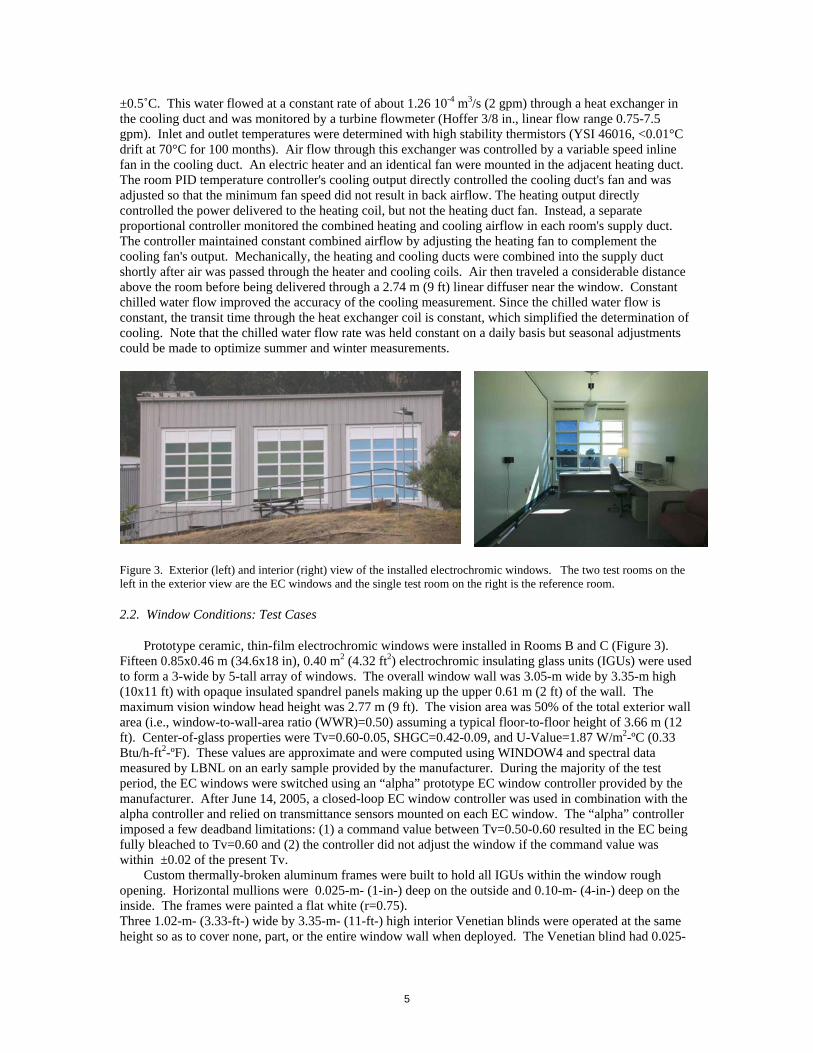
Figure 3. Exterior (left) and interior (right) view of the installed electrochromic windows. The two test rooms on the left in the exterior view are the EC windows and the single test room on the right is the reference room.

2.2. Window Conditions: Test Cases

Prototype ceramic, thin-film electrochromic windows were installed in Rooms B and C (Figure 3). Fifteen 0.85x0.46 m (34.6x18 in), 0.40 m2 (4.32 ft2) electrochromic insulating glass units (IGUs) were used to form a 3-wide by 5-tall array of windows. The overall window wall was 3.05-m wide by 3.35-m high (10x11 ft) with opaque insulated spandrel panels making up the upper 0.61 m (2 ft) of the wall. The maximum vision window head height was 2.77 m (9 ft). The vision area was 50% of the total exterior wall area (i.e., window-to-wall-area ratio (WWR)=0.50) assuming a typical floor-to-floor height of 3.66 m (12 ft). Center-of-glass properties were Tv=0.60-0.05, SHGC=0.42-0.09, and U-Value=1.87 W/m2-ºC (0.33 Btu/h-ft2-ºF). These values are approximate and were computed using WINDOW4 and spectral data measured by LBNL on an early sample provided by the manufacturer. During the majority of the test period, the EC windows were switched using an “alpha” prototype EC window controller provided by the manufacturer. After June 14, 2005, a closed-loop EC window controller was used in combination with the alpha controller and relied on transmittance sensors mounted on each EC window. The “alpha” controller imposed a few deadband limitations: (1) a command value between Tv=0.50-0.60 resulted in the EC being fully bleached to Tv=0.60 and (2) the controller did not adjust the window if the command value was within ±0.02 of the present Tv.

Custom thermally-broken aluminum frames were built to hold all IGUs within the window rough opening. Horizontal mullions were 0.025-m- (1-in-) deep on the outside and 0.10-m- (4-in-) deep on the inside. The frames were painted a flat white (r=0.75). Three 1.02-m- (3.33-ft-) wide by 3.35-m- (11-ft-) high interior Venetian blinds were operated at the same height so as to cover none, part, or the entire window wall when deployed. The Venetian blind had 0.025-

6

m- (1-in-) wide, curved, matte white, horizontal slats. When deployed, the slat angle was set to just block direct sun: ~45º from horizontal so that the lower edge of the slat was toward the exterior.

2.3. Window Conditions: Reference Case

Reference case windows were double-pane spectrally selective low-E windows. Center-of-glass properties were Tv=0.42, SHGC=0.219, U-Value=1.408 W/m2-ºC (0.25 Btu/h-ft2-ºF). The insulating glass units (IGU) were fabricated with the same dimensions and spacers as the test electrochromic IGUs. These reference windows were installed in Room A with the same framing and interior Venetian blind configuration as the test cases.

Figure 4. Plan view of a test room showing position of the lighting fixtures, photosensor, and interior work plane illuminance sensors (+ symbol).

2.4. Lighting Condition

Two 0.61x1.22-m (2x4 ft) pendant, indirect-direct (~95%, 5%) fixtures with four T8 (25-mm) 32-W fluorescent lamps and one continuous dimmable electronic ballast per fixture were used in each room. The two fixtures were placed along the centerline of the window with the south ends of the first and second fixture located 0.60 m and 2.74 m (2 and 9 ft) from the window wall, respectively (Figure 4). The fixtures were suspended 0.76 m (2.5 ft) from the ceiling. At full power, the lighting power density (LPD) was 18.7 W/m2 (1.73 W/ft2) and the maximum work plane illuminance was 715 lux (66 fc). For the setpoint work plane illuminance of 540 lux (50 fc), the LPD was 14.9 W/m2 (1.39 W/ft2). The range of dimming for these ballasts were 10-100% of full light output and 28-100% of full power.

Two shielded photosensors (Perkin Elmer VT5051B, 0.02% per °C) were placed at the south end of the second light fixture, 2.73 m (9 ft) from the window wall and flush with the bottom of the fixture, 2.54 m (8.3 ft) above the finished floor. One photosensor had a 60° cone of view and was pointed downward, normal to the floor. Its view was defined by a circular area on the floor with a radius of 1.47 m (4.8 ft). The second shielded photosensor was directed at the mid- to upper portion of the back wall to avoid influence of low-angle direct sun that occurred between the fall and spring equinox. The photosensors’ unconditioned voltage signals were processed via software and used to control the dimming ballast. If the two readings differed by more than 5%, then the rear wall photosensor was used for control. Dimming levels were determined using closed-loop proportional control.

2.5. Tested Configurations: Reference Cases

Two reference cases were defined: (1) static glazing with no interior shades and (2) static glazing with interior Venetian blinds covering the full height of the window. The dimmable electric lighting system was automatically controlled every 30 s to supplement available daylight so as to maintain a minimum horizontal work plane illuminance of 510 lux (47 fc) within the rear zone of the test space.

7

2.6. Tested Configurations: Test Cases

The test case configuration in Rooms B and C was defined with a dynamic electrochromic window and the same dimmable daylighting control as the reference case. Several window configurations were tested: (1) all 15 EC windows were controlled using the same algorithm (1-zone), (2) the upper row of EC windows were controlled as one zone and the lower four rows of EC windows were controlled as a second zone (“2-zone 1-4”), and (3) the upper two rows of EC windows were controlled as one zone and the lower three rows were controlled as a second zone (“2-zone 2-3”). Venetian blinds were either fully drawn up or were lowered to cover the full window wall (1-zone case), the upper row of EC windows (2-zone 1-4 case), or the upper two rows of EC windows (2-zone 2-3 case).

Two control algorithms were used to switch the EC windows. For the “daylight (d)” mode, the transmittance of the EC window was automatically adjusted every 1 min to provide an average work plane daylight illuminance of 540-600 lux (50-56 fc) within the rear zone of the test space. The supervisory control system was implemented using National Instruments LabView software and interfaced with the manufacturer's EC window controller or window-mounted transmittance sensors. Proper switching of the window was accomplished using closed-loop proportional control via the same ceiling-mounted photosensors used for the electric lighting. For the “glare (dg5)” mode, the EC windows were switched to the maximum colored state (Tv=0.05) when the incident south vertical illuminance exceeded 30,000 lux and for all other times, the daylight mode was used. A value of 20,000 lux was found to correlate to a near 100% probability that the occupants would draw the blinds over the EC windows in a companion user assessment field study (Clear et al. 2005) and a window luminance of 3000 cd/m2 was found to correlate to a 75% probability of drawing the blinds. A less conservative threshold value was used in combination with partially-lowered Venetian blinds. After May 21, 2005, a provision was added to the glare mode where if the solar profile angle was greater than 75º, then the control system would switch to the daylight mode (“dg5:75”). This increased interior daylight levels during summer midday hours. The daylight mode was used with and without interior shades in the 1-zone window configuration, and in the upper window zones in the 2-zone configurations. The glare mode was used with and without interior shades in the 1-zone window configuration, and in the lower window zones in the 2-zone configurations. Table 1 provides a list of the reference versus test configurations. Table 1Comparative Test Conditions

Case Reference case Test case Test caseAlgorithm Shading condition

1 no blind d no blind2 no blind dg5 no blind3 VB1.45 d no blind4 VB1.45 d VB1.455 VB1.45 dg5 no blind6 VB1.45 1d.4dg5:75 VB020.457 VB1.45 2d.3dg5:75 VB040.45 VB020.45: blind lowered over top row of EC windows, VB040.45: blind lowered over top two rows of EC

windows, VB1.45: blind lowered over full window. All positions with slat angle set to 45°. EC control modes: d: daylight, dg5: daylight + glare (Tv=0.05), dg5:75 same as dg5 but switches to the glare

mode when solar profile angle is less than 75°. 1d.4dg5: 2 zones with one row of EC windows in upper zone and four rows of EC windows in lower zone. 2d.3dg5: 2 zones with two rows of EC windows in upper zone and three rows of EC windows in lower zone.

2.7. Monitored Data and Analysis

Data were collected over 20 months from May 1, 2004 to December 15, 2005 over a 24-h period using the LabView National Instruments data acquisition software. All data were recorded in Standard Local Time. Each test room contained over 100 sensors measuring horizontal work plane illuminance, vertical

8

illuminance, power consumption of all plug loads and mechanical equipment, cooling load, interior air temperature, window transmittance and other information pertaining to the status of the dynamic window and lighting system. Exterior conditions were also measured. Horizontal and vertical radiation and illuminance were monitored on the roof and south façade, respectively. Outdoor dry-bulb temperature was measured high on the north façade, using a shielded thermistor (±0.2°C YSI 44016). Lighting energy and cooling load data were sampled every one second then averaged and recorded every one minute. All other data were sampled and recorded every one minute. Detailed descriptions of the daylighting and EC window monitoring instrumentation are given in Lee et al. (2006).

Data were filtered prior to inclusion in the dataset. Data were eliminated if the room was occupied or special tests were being conducted, if any of the instrumentation or HVAC systems were not operating properly, or if the EC window or lighting system was not operating as intended. If the daylighting control system did not maintain the average rear zone work plane illuminance above 90% of the setpoint level (459 lux, 43 fc) for greater than 90% of the day, then data were not included (97% of the data were retained). To eliminate days when poor EC operations occurred, the percentage of day that the monitored EC transmittance was within 0.10 of the desired Tv command value was tallied for each of the 15 windows. If 13 of the 15 EC windows maintained proper EC control for greater than 80% of the day, then the day was included in the analysis.

2.8. Lighting Energy Use

Electric lighting power consumption was measured in each test room with watt transducers (Ohio Semitronics GW5) that were accurate to 0.2% of reading. Daily lighting energy use was the sum of 1-min data over the 12-h period from 6:00-18:00. Note that the lighting energy use would be approximately the same for a smaller window area (WWR=0.40), since a desk blocked the lower row of windows.

2.9. Heating and Cooling Heat Flow

The cooling or heating demand due to the window was measured for each test room. Measurements were corrected for thermal and room-to-room variations using a static thermal model. The resulting “dynamic net heat flow”, or standardized cooling demand, is expected to represent, on average, only the effects of solar gain (including internal solar storage) on a standardized room.

To compare the thermal loads resulting from different fenestrations and/or control strategies, it is necessary to account for heat flows that result from differences among the test rooms that are irrelevant to the fenestration comparisons. Since the rooms were built with standard construction techniques, some differences in thermal properties are expected. In addition, each room is separately controlled by control systems that are less than perfect, and conditioned air is supplied to each by separate duct systems. This means that there are likely to be differences in the internal air temperatures of the rooms, even when they are nominally set to the same temperature. In addition, duct losses between the point where applied heating or cooling is measured and the entrance to the test room could differ from room to room, and there could be miscalibrations of the measurement apparatus.

Nighttime calibration tests, conducted with the mechanical system off, were used to ascertain the comparability between the two rooms given instrumental error, differences in construction, the rooms’ relative position to the exterior and interior environment, and the mechanical systems' operation. Static nighttime tests (where in some tests, the entire window was covered with insulation in all three rooms) were conducted to determine cooling and heating system efficiencies, floor, exterior wall, and window UA values, ceiling and interior wall UA values, and sensitivity to changes in static condition. Dynamic nighttime tests were also conducted. Dynamic tests were intended to measure the effect of heat storage in the building envelope but also provided considerable information about the performance of the control system. These included a control system response test, a radiant heater pulse test, a lighting pulse test and a test to determine radiant and light losses through the window. While these tests gave information about the time response of the test chambers, and in particular did not yield any evidence of significant differences between the time responses of the two chambers, it was not possible to determine empirically the thermal mass or solar response factors of the chambers. Hence, the data presented here are the power demands, including the response of the two nominally identical chambers. Solar tests were conducted during the day to do an equal glazing transmittance comparison, an equal weighted transmittance comparison, and to

9

determine floor absorption, floor reflectance, and sill/frame absorption and reflection. The results of these calibration tests have been given in a separate report (Klems 2004).

The cooling load due to the window was then calculated as DPµ = Pµ

M − PµP (1)

where µ = a,b,c is a subscript identifying the particular room, PM is the measured room power,

and PP is the room power predicted from the static model. The measured power is calculated as

Pµ = εµCµ -ηµHµ - Lµ - Fµ -Pµ (2)

In this equation, H , L, F and P are measured heat added by the heating system, lighting power, fan power, and in-room electric power respectively. These were directly measured with watt transducers. The quantities ε and η are constants determined in the calibration (and correct for effects such as duct losses and small miscalibrations of the heating or cooling measurement systems) and C is determined from the equation

C=ρcP ⋅ f ⋅ Tex − Ten( ) (3)

and the measured coolant flow rate ( f ), entering temperature (Ten ) and exit temperature (Tex ). The predicted power is determined as

P = P0 +UAW ⋅ (TE − TI ) +UAF ⋅ (TU − TI ) +UAG ⋅ (TG − TI ) (4) in which the measured quantities are the temperatures (E=outdoor, I=indoor, U=underfloor plenum,

and G=guard) and all other quantities are constants determined from the calibration tests. To determine the net heat flow due to the lighting and solar gain, the lighting power was added to the result from equation (2) above since the pendant lighting fixtures used in these tests contribute 100% of their heat to the room interior.

2.10. Load Definitions

Although the measurements were sampled every 1 s then averaged over 1 min, the net heat flow was always determined over longer periods. Due to thermal storage in the HVAC elements, etc., the measurements probably do not represent the room net heat flow reliably for period shorter than approximately 10 min. If we consider C to be a measured quantity rather than one derived from two measurements, then since all of the other equations are linear, averaging the dynamic net heat flow over different periods is the same as averaging the underlying measured quantities over the same periods. (In fact, although a measured quantity, the fluid flow rate is effectively constant on the time scale over which the other quantities vary significantly, and therefore the time average of C is effectively the time average of the fluid temperature difference.)

The average hourly cooling load was determined for each room by averaging the 1-min data over an hour then computing the hourly net heat flow or cooling load. The daily cooling load due to the window, Qw, and the daily cooling load due to the window and the lights, Qw+l, were then computed over the 12-h period defined by 6:00-18:00. Peak cooling load due to the window was defined as the measured load that occurred two hours after the hour when the vertical solar irradiance level was at its peak. The peak daily cooling load did occur at different times in each room, but the mechanism driving peak loads was solar irradiance and this analysis focuses on the difference in coincident peak solar loads produced by the EC window (EC windows modulate only solar heat gains, not U-value). Differences in maximum daily peak load and coincident peak load were small, with the latter method producing less scatter.

As should be apparent from the above discussion, the terms “instantaneous heat flow”, “peak load” and “average load” refer to averages taken over time periods of different lengths, and to this extent are matters of definition (as of course they are in the discussion of energy usage in an actual or simulated building). A true instantantaneous chamber heat flow is not measurable by this (or any other calorimetric) facility, because the systems which make the measurement have their own intrinsic thermal mass which cannot be made completely negligible. As stated above, in this facility measurements made over sufficiently short time periods to be termed instantaneous (or, pseudo-instantaneous) do not reliably characterize the chamber behavior, because of transient errors that cancel out over larger averaging periods. When the dynamic net heat flow is averaged it might be termed the dynamic demand (e.g., averaging over an hour would give a

10

dynamic demand, the maximum value of which would be termed the dynamic peak demand; similarly, a long-period average would yield the average dynamic demand, or average dynamic load).

The static model of Equation 4 was developed with pseudostatic measurements, in which the variations in conditions were sufficiently slow so that heat storage effects became negligible. Subtracting off this (calculated) static power to produce the dynamic net heat flow is simply an accounting device that enables measurements made under different average conditions (indoor-outdoor temperature difference, difference between chamber temperature and guard temperature, etc.) to be compared on the same footing. In the process, the average thermal heat flow through the window is also subtracted off. However, rapid changes during the daytime, due most directly to solar radiation, but also including consequent heating of the glazings and coincident rapid outdoor temperature changes, appear, modified by the chamber time response, in the dynamic net heat flow (averaged over the appropriate period). This is why it is important that comparisons are made between different glazing conditions applied simultaneously to the three chambers, and why the chambers were made as representative of a realistic office environment as possible

Error estimates, described in more detail below, are derived by considering the probable variances of the (average) measured quantities (random errors) or parameters (systematic errors) in the above equations and determining the resultant probable variance of the dynamic net power.

2.11. Error in Lighting Power Use Between Test Rooms

Nighttime fluorescent calibrations were performed where the lighting levels were stepped over the full dimming range in order to quantify the relationship between light output and power consumption. Differences in lighting power consumption between all test rooms were no greater than 1.1 W if the average work plane illuminance was between 100-550 lux. Differences were more difficult to characterize for light levels less than 100 lux but these differences were still small (<1 W). This was within the measurement accuracy of the watt transducers (0.2% of reading). Between-room error in daily lighting energy use due to test room position was less than 1%, as documented in Lee et al. 2006.

2.12. Estimated Error or Uncertainty in Thermal Load

All measurements are imperfect representations of reality; the difference between a measurement result and the “true” value (which is unknowable) is the error of the measurement. By statistical techniques, one can estimate how close the measured value should be to the true value. This is the uncertainty of the measurement, usually called the error estimate. The data gathered during the calibration measurements were used to make models of the measurement processes for generating error estimates.

There are two types of error that need to be considered: errors resulting directly from measurement and errors introduced by the standardization. These are termed “random” and “systematic” errors respectively and behave differently as one averages over longer times. Generally, the uncertainty from random errors decreases as one averages over longer times, while that from systematic errors is relatively unaffected.

The random error estimate for heating power is proportional to the heating power. The error estimate for the cooling power has two parts: a constant error at low cooling powers and an error proportional to the cooling power, which dominates at high cooling powers. These two error estimates are combined to give the random measurement uncertainty for the cooling demand. Since both the heating and cooling powers vary with, for instance, time of day, this uncertainty also varies.

The systematic error estimate covers two types of problems with the standardization formula. First, the parameters used in the formula were determined by the calibration experiments, and therefore they have uncertainties arising from the measurement errors in those experiments. This results in a systematic error estimate that can be calculated by a rather complicated but perfectly definite formula involving the measured heating and cooling powers; the systematic error therefore varies with time, but for reasons completely different from the random errors—here, different times do not represent independent events.

Second, the static model used in the standardization can fail to represent the situation adequately for a variety of reasons. A second systematic error estimate is used to estimate the effect of this. It was determined by examining the behavior of the rooms late at night for a month following the calibration. Late at night the standardized cooling demand should be zero, so the measured values during this period should be consistent with zero given the estimates of random and systematic error. This proved not to be quite true (due to errors of unknown origin), so an additional systematic error estimate was necessary. This

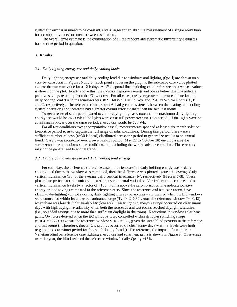
11

systematic error is assumed to be constant, and is larger for an absolute measurement of a single room than for a comparative measurement between two rooms.

The overall error estimate is the combination of all the random and systematic uncertainty estimates for the time period in question.

3. Results

3.1. Daily lighting energy use and daily cooling loads

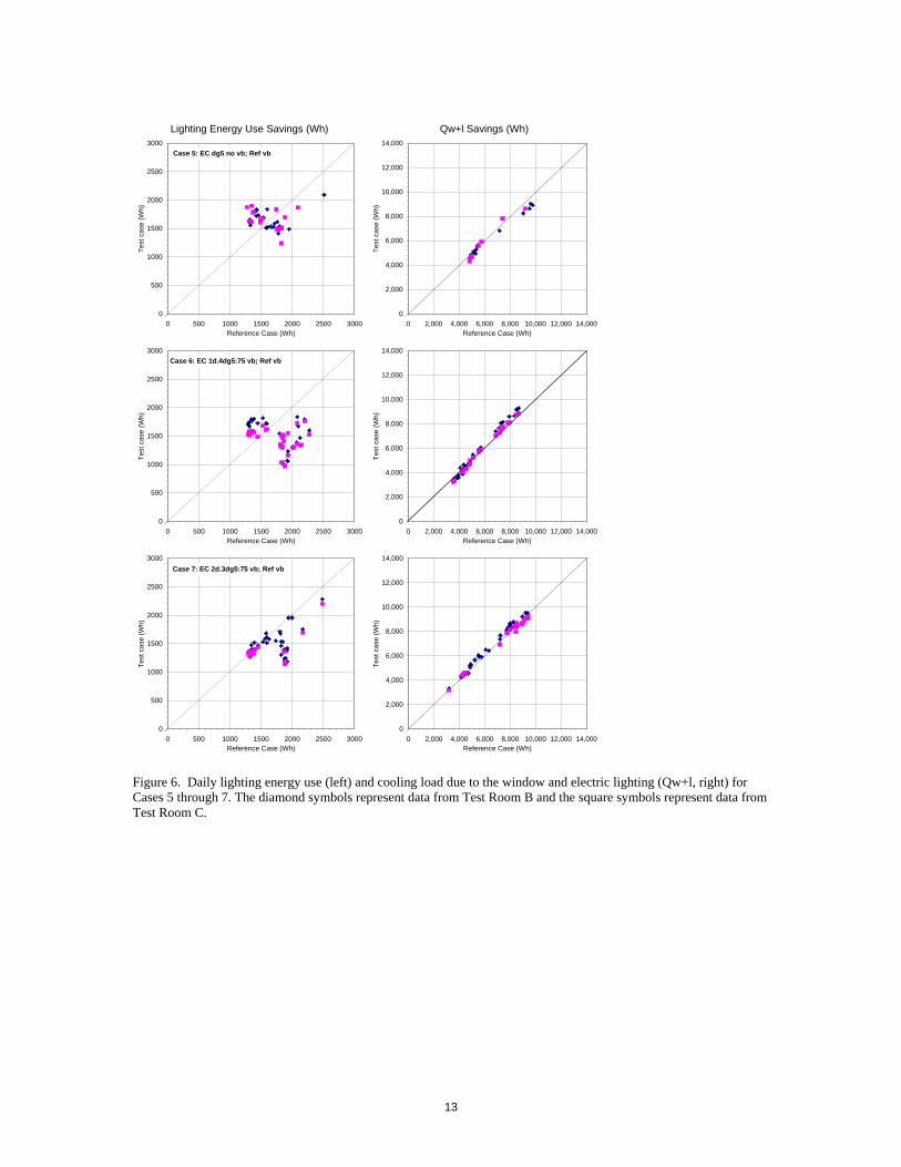
Daily lighting energy use and daily cooling load due to windows and lighting (Qw+l) are shown on a case-by-case basis in Figures 5 and 6. Each point shown on the graph is the reference case value plotted against the test case value for a 12-h day. A 45º diagonal line depicting equal reference and test case values is shown on the plot. Points above this line indicate negative savings and points below this line indicate positive savings resulting from the EC window. For all cases, the average overall error estimate for the daily cooling load due to the windows was 382±160 Wh, 170±35 Wh, and 194±39 Wh for Rooms A, B, and C, respectively. The reference room, Room A, had greater hysteresis between the heating and cooling system operations and therefore had a greater overall error estimate than the two test rooms.

To get a sense of savings compared to a non-daylighting case, note that the maximum daily lighting energy use would be 2630 Wh if the lights were on at full power over the 12-h period. If the lights were on at minimum power over the same period, energy use would be 720 Wh.

For all test conditions except comparative case 6, measurements spanned at least a six-month solstice-to-solstice period so as to capture the full range of solar conditions. During this period, there were a sufficient number of days (n=30 is ideal) distributed across the period to generalize results to an annual trend. Case 6 was monitored over a seven-month period (May 22 to October 18) encompassing the summer solstice-to-equinox solar conditions, but excluding the winter solstice condition. These results may not be generalized to annual trends.

3.2. Daily lighting energy use and daily cooling load savings

For each day, the difference (reference case minus test case) in daily lighting energy use or daily cooling load due to the window was computed, then this difference was plotted against the average daily vertical illuminance (Ev) or the average daily vertical irradiance (Iv), respectively (Figures 7-8). These plots relate performance quantities to exterior environmental variables. Vertical irradiance correlated to vertical illuminance levels by a factor of ~100. Points above the zero horizontal line indicate positive energy or load savings compared to the reference case. Since the reference and test case rooms have identical daylighting control systems, daily lighting energy use savings were derived when the EC windows were controlled within its upper transmittance range (Tv=0.42-0.60 versus the reference window Tv=0.42) when there was less daylight availability (low Ev). Lesser lighting energy savings occurred on clear sunny days with high daylight availability when both the reference and test rooms reached daylight saturation (i.e., no added savings due to more than sufficient daylight in the room). Reductions in window solar heat gains, Qw, were derived when the EC windows were controlled within its lower switching range (SHGC=0.22-0.09 versus the reference window SHGC=0.22, given the same blind position in the reference and test rooms). Therefore, greater Qw savings occurred on clear sunny days when Iv levels were high (e.g., equinox to winter period for this south-facing facade). For reference, the impact of the interior Venetian blind on reference case lighting energy use and solar heat gains is shown in Figure 9. On average over the year, the blind reduced the reference window’s daily Qw by ~13%.

12

Lighting Energy Use Savings (Wh) Qw+l Savings (Wh)

Case 1: EC d no vb; Ref no vb

0

500

1000

1500

2000

2500

3000

0 500 1000 1500 2000 2500 3000Reference Case (Wh)

Test

cas

e (W

h)

0

2,000

4,000

6,000

8,000

10,000

12,000

14,000

0 2,000 4,000 6,000 8,000 10,000 12,000 14,000Reference Case (Wh)

Test

cas

e (W

h)

Case 2: EC dg5 no vb; Ref no vb

0

500

1000

1500

2000

2500

3000

0 500 1000 1500 2000 2500 3000Reference Case (Wh)

Test

cas

e (W

h)

0

2,000

4,000

6,000

8,000

10,000

12,000

14,000

0 2,000 4,000 6,000 8,000 10,000 12,000 14,000Reference Case (Wh)

Test

cas

e (W

h)

Case 3: EC d no vb; Ref vb

0

500

1000

1500

2000

2500

3000

0 500 1000 1500 2000 2500 3000Reference Case (Wh)

Test

cas

e (W

h)

0

2,000

4,000

6,000

8,000

10,000

12,000

14,000

0 2,000 4,000 6,000 8,000 10,000 12,000 14,000Reference Case (Wh)

Test

cas

e (W

h)

Case 4: EC d vb; Ref vb

0

500

1000

1500

2000

2500

3000

0 500 1000 1500 2000 2500 3000Reference Case (Wh)

Test

cas

e (W

h)

0

2,000

4,000

6,000

8,000

10,000

12,000

14,000

0 2,000 4,000 6,000 8,000 10,000 12,000 14,000Reference Case (Wh)

Test

cas

e (W

h)

Figure 5. Daily lighting energy use (left) and cooling load due to the window and electric lighting (Qw+l, right) for Cases 1 through 4. The diamond symbols represent data from Test Room B and the square symbols represent data from Test Room C.

13

Lighting Energy Use Savings (Wh) Qw+l Savings (Wh) Case 5: EC dg5 no vb; Ref vb

0

500

1000

1500

2000

2500

3000

0 500 1000 1500 2000 2500 3000Reference Case (Wh)

Test

cas

e (W

h)

0

2,000

4,000

6,000

8,000

10,000

12,000

14,000

0 2,000 4,000 6,000 8,000 10,000 12,000 14,000Reference Case (Wh)

Test

cas

e (W

h)

Case 6: EC 1d.4dg5:75 vb; Ref vb

0

500

1000

1500

2000

2500

3000

0 500 1000 1500 2000 2500 3000Reference Case (Wh)

Test

cas

e (W

h)

0

2,000

4,000

6,000

8,000

10,000

12,000

14,000

0 2,000 4,000 6,000 8,000 10,000 12,000 14,000Reference Case (Wh)

Test

cas

e (W

h)

Case 7: EC 2d.3dg5:75 vb; Ref vb

0

500

1000

1500

2000

2500

3000

0 500 1000 1500 2000 2500 3000Reference Case (Wh)

Test

cas

e (W

h)

0

2,000

4,000

6,000

8,000

10,000

12,000

14,000

0 2,000 4,000 6,000 8,000 10,000 12,000 14,000Reference Case (Wh)

Test

cas

e (W

h)

Figure 6. Daily lighting energy use (left) and cooling load due to the window and electric lighting (Qw+l, right) for Cases 5 through 7. The diamond symbols represent data from Test Room B and the square symbols represent data from Test Room C.

14

Lighting energy savings (Wh) Qw+l savings (Wh) Lighting + Qw+l/COP savings (Wh) 1

-1000

-800

-600

-400

-200

0

200

400

600

800

1000

0 30,000 60,000

Avg daily exterior vertical illuminance (lux)

Dai

ly li

ghtin

g en

ergy

use

sav

ings

(Wh)

-3000

-2400

-1800

-1200

-600

0

600

1200

1800

2400

3000

0 300 600

Avg daily vertical irradiance (W/m2)

Dai

ly Q

w+l

sav

ings

(Wh)

-1000

-800

-600

-400

-200

0

200

400

600

800

1000

0 30,000 60,000

Avg daily exterior vertical illuminance (lux)

Dai

ly c

oolin

g +

light

ene

rgy

savi

ngs

(Wh)

2

-1000

-800

-600

-400

-200

0

200

400

600

800

1000

0 30,000 60,000

Avg daily exterior vertical illuminance (lux)

Dai

ly li

ghtin

g en

ergy

use

sav

ings

(Wh)

-3000

-2400

-1800

-1200

-600

0

600

1200

1800

2400

3000

0 300 600

Avg daily vertical irradiance (W/m2)

Dai

ly Q

w+l

sav

ings

(Wh)

-1000

-800

-600

-400

-200

0

200

400

600

800

1000

0 30,000 60,000

Avg daily exterior vertical illuminance (lux)

Dai

ly c

oolin

g +

light

ene

rgy

savi

ngs

(Wh)

3

-1000

-800

-600

-400

-200

0

200

400

600

800

1000

0 30,000 60,000

Avg daily exterior vertical illuminance (lux)

Dai

ly li

ghtin

g en

ergy

use

sav

ings

(Wh)

-3000

-2400

-1800

-1200

-600

0

600

1200

1800

2400

3000

0 300 600

Avg daily vertical irradiance (W/m2)

Dai

ly Q

w+l

sav

ings

(Wh)

-1000

-800

-600

-400

-200

0

200

400

600

800

1000

0 30,000 60,000

Avg daily exterior vertical illuminance (lux)

Dai

ly c

oolin

g +

light

ene

rgy

savi

ngs

(Wh)

4

-1000

-800

-600

-400

-200

0

200

400

600

800

1000

0 30,000 60,000

Avg daily exterior vertical illuminance (lux)

Dai

ly li

ghtin

g en

ergy

use

sav

ings

(Wh)

-3000

-2400

-1800

-1200

-600

0

600

1200

1800

2400

3000

0 300 600

Avg daily vertical irradiance (W/m2)

Dai

ly Q

w+l

sav

ings

(Wh)

-1000

-800

-600

-400

-200

0

200

400

600

800

1000

0 30,000 60,000

Avg daily exterior vertical illuminance (lux)

Dai

ly c

oolin

g +

light

ene

rgy

savi

ngs

(Wh)

Figure 7. Average daily vertical illuminance or irradiance versus daily lighting energy savings (left), daily cooling load savings due to solar heat gains and lighting (middle), and net daily energy savings (right) for Cases 1 (top) through 4 (bottom). diamonds: Room B; pink squares: Room C.

15

Lighting energy savings (Wh) Qw+l savings (Wh) Lighting + Qw+l/COP savings (Wh)

5

-1000

-800

-600

-400

-200

0

200

400

600

800

1000

0 30,000 60,000

Avg daily exterior vertical illuminance (lux)

Dai

ly li

ghtin

g en

ergy

use

sav

ings

(Wh)

-3000

-2400

-1800

-1200

-600

0

600

1200

1800

2400

3000

0 300 600

Avg daily vertical irradiance (W/m2)

Dai

ly Q

w+l

sav

ings

(Wh)

-1000

-800

-600

-400

-200

0

200

400

600

800

1000

0 30,000 60,000

Avg daily exterior vertical illuminance (lux)

Dai

ly c

oolin

g +

light

ene

rgy

savi

ngs

(Wh)

6

-1000

-800

-600

-400

-200

0

200

400

600

800

1000

0 30,000 60,000

Avg daily exterior vertical illuminance (lux)

Dai

ly li

ghtin

g en

ergy

use

sav

ings

(Wh)

-3000

-2400

-1800

-1200

-600

0

600

1200

1800

2400

3000

0 300 600

Avg daily vertical irradiance (W/m2)

Dai

ly Q

w+l

sav

ings

(Wh)

-1000

-800

-600

-400

-200

0

200

400

600

800

1000

0 30,000 60,000

Avg daily exterior vertical illuminance (lux)

Dai

ly c

oolin

g +

light

ene

rgy

savi

ngs

(Wh)

7

-1000

-800

-600

-400

-200

0

200

400

600

800

1000

0 30,000 60,000

Avg daily exterior vertical illuminance (lux)

Dai

ly li

ghtin

g en

ergy

use

sav

ings

(Wh)

-3000

-2400

-1800

-1200

-600

0

600

1200

1800

2400

3000

0 300 600

Avg daily vertical irradiance (W/m2)

Dai

ly Q

w+l

sav

ings

(Wh)

-1000

-800

-600

-400

-200

0

200

400

600

800

1000

0 30,000 60,000

Avg daily exterior vertical illuminance (lux)

Dai

ly c

oolin

g +

light

ene

rgy

savi

ngs

(Wh)

Figure 8. Average daily vertical illuminance or irradiance versus daily lighting energy saving (left), daily cooling load savings due to solar heat gains and lighting (middle), and net daily energy savings (right) for Cases 5 (top) through 7 (bottom). Blue diamonds: Room B; pink squares: Room C

Note that when the two energy quantities are considered simultaneously, the net effect can be positive overall savings. For example, in Figure 7 Case 1, on a clear sunny winter day (Iv>300 W/m2, Ev>30,000 lux), daily lighting energy use savings were low while cooling load reductions were high. The net savings will depend on the efficacy of the HVAC system – if a simple loads to HVAC plant coefficient-of-performance (COP) value of 3 is assumed, for example, the net energy savings for Cases 1 and 3 (1-zone daylight control of EC windows) are positive across the entire range of solar conditions. One can also determine roughly when such savings occur based on the incident solar radiation levels (e.g., see Figure 10, 380-500 W/m2 correspond to equinox to winter solstice clear sky conditions; less than 150 W/m2 corresponds to cloudy conditions). The y-axes in Figures 7 and 8 have been scaled so that the lighting energy savings can be compared to the cooling load savings (assuming a COP=3). Savings are given for a 13.86 m2 (150 ft2) office space. Daily savings of 180 Wh over the 12-h period are equivalent to an average reduction in site energy use of 0.1 W/ft2-floor for this south-facing 4.6-m (15-ft) deep perimeter zone.

16

This particular type of EC window requires a small trickle charge to switch and maintain the window transmittance at a steady state. Other types of EC windows require power only to switch the EC to a different transmittance level, and when unpowered, will maintain the current level of transmittance with minimal change over several days. The daily power consumption used to maintain the EC windows at a steady state and switch the windows was not included in this net savings. EC average daily power consumption levels for this prototype solution will erode the above savings by ~55-120 Wh or 0.03-0.07 W/ft2-floor (includes steady-state power use and peak power use when switching to different transmittance levels). These consumption levels can be reduced to 25-30% of current levels, if the control circuitry and power source are designed more efficiently.

0

500

1,000

1,500

2,000

2,500

3,000

3,500

0 10,000 20,000 30,000 40,000 50,000 60,000

Exterior vertical illuminance (lux)

Dai

ly li

ghtin

g en

ergy

use

(Wh)

no blind fully lowered blind

fully lowered blindy = 15.108xR2 = 0.9536

no blindy = 17.431xR2 = 0.9755

0

1,000

2,000

3,000

4,000

5,000

6,000

7,000

8,000

9,000

10,000

0 100 200 300 400 500 600

Exterior vertical irradiance (W/m2)

Coo

ling

load

due

to w

indo

w s

olar

hea

t gai

ns (W

h)

Figure 9. Effect of interior Venetian blind on window performance. Daily lighting energy use and cooling load due to solar heat gains, Qw, for the reference spectrally-selective window (SHGC=0.22) with and without a fully-lowered matte-white Venetian blind with 2.54-cm (1-inch) slats tilted to 45° (view of ground from inside). Data were computed for 6:00-18:00 and are given for the full 20-month monitored period. Minimum daily lighting energy use is 720 Wh.

0

10,000

20,000

30,000

40,000

50,000

60,000

03/21/04 06/21/04 09/21/04 12/22/04 03/24/05 06/24/05 09/24/05 12/25/05Date (month/day/year)

Ext

erio

r ver

tical

illu

min

ance

(lux

)

Figure 10. Average daily exterior vertical illuminance levels monitored on a south-facing façade. The upper points forming the sinusoidal shape are the clear sunny days with lowest levels (~20,000 lux) occurring around the summer solstice and highest levels occurring around the winter solstice (54,000 lux).

17

3.3. Peak demand reductions in lighting and cooling loads

A control system of this type is likely to be connected to the central building management control system (BMCS), in which case the facility manager can be provided with several peak demand reduction options: (1) allow the EC window-daylighting control system to operate as specified, (2) curtail peak loads according to cost criteria (e.g., time-of-use rate schedules) without significantly affecting occupant comfort, or (3) implement a demand-response mode, which may inconvenience the occupants. To quantify peak load reduction potential, one must define which of the above control scenarios is being considered. For a 111 km2 (1.2 Mft2) commercial office building that we are currently involved with, for example, the owner is willing to turn off the electric lights in the perimeter zone using the BMCS, have occupants use their 7-W light-emitting diode (LED) task lights if needed, and control the automated interior shades to minimize window heat gains during critical demand-response periods when black-outs are impending. Applying such a scenario to this dataset (option 3), lighting peak demand reductions would be 0%, assuming that the reference case has the same ability to turn off the lights, and cooling peak load reductions due to window solar heat gains (EC at its maximum colored state, Cases 2 and 5) would be 19-26% maximum (clear sunny days) or 10-17% on average, where the range in savings is dependent on whether the reference case shades are up or down. For BMCS control options (1) and (2), one must determine the likely reference case shade position during peak load conditions, then select the EC control algorithm that balances peak load reductions in lighting versus cooling due to window heat gains for the given solar condition. While the single-zone glare control mode (Cases 2 and 5) yields the greatest reduction in peak cooling load, trade-offs with lighting energy use must be considered. For this large-area window, the EC glare mode (Tv at minimum) may still admit sufficient daylight to enable the electric lighting to be turned off.

3.4. Sources of error

The scatter in the data may be due to a number of factors: day-to-day variations in sky condition, seasonal differences in solar conditions, etc. Outlier data were investigated to determine if there were underlying malfunctions in the window or lighting control systems or in the sensors, HVAC, or data acquisition system. Another cause of scatter in the data is likely the variation in EC operations from the intended control objective. As described in the Method section above, we established criteria for determining whether the EC windows were operating largely as intended. This criteria was established to eliminate days when there were problems with EC control but also to retain data. In an earlier field study assessment of these EC windows (Lee et al. 2006), we found that the EC devices had good within-pane and between-pane (side-by-side EC windows) uniformity, responded consistently when prompted to switch, and switched generally within 1-5 min over a 5-month test period following initial installation. These same windows have now been tested over a total 2.75-year installed period. During this period, the accuracy and speed of switching to intermediate and end states declined for some of the EC windows. For a few windows, the transmittance of the end states changed by 0.05-0.15 – e.g., the bleached or colored end state transmittance became lower or higher. For a few windows, the EC window took longer to reach its requested state (20 min or longer). The manufacturer attributed these problems to the early development stage of their alpha intermediate-state control design and potentially to unanticipated frequent minute-to-minute switching of the EC windows to meet control system objectives. We speculate that the initial electrical characterization (e.g., correlation of the EC window’s current-to-voltage waveform to a given transmittance level) may also have drifted causing under- or overdrive of the EC windows. Our evaluation of the EC window operations relied on a transmittance sensor mounted on each EC window and on visual inspection. These sensors were designed for the purpose of providing approximate relative, not absolute transmittance data. Degradation of these sensors due to dirt or other factors may also partially explain the shifts in the end state transmittance range. After the switch to closed-loop control June 14, 2005, the accuracy and speed of switching returned to its initial installed performance, confirming the manufacturer’s rationale.

The end state transmittances for a few of the windows shifted, contributing to differences in performance between Rooms B and C, most notably during approximately the last six months of the test period. This affected the data for Cases 6 and 7. In Room B, two of the 15 lower EC windows fully bleached but did not color as deeply (Tv≅0.10 minimum). In Room C, two of the 15 mid-height EC windows fully colored but did not fully bleach (Tv≅0.45-0.55 maximum). When controlled using the same algorithm, the daily cooling loads Qw and Qw+l of Room B were 2±3% and 3±2% (n=43) greater than

18

Room C on average, respectively, during this period. The peak cooling load of Room B was 3±2% greater than Room C. Between-room differences in cooling load can be seen on the plots in Figure 8 for Cases 6 and 7 (most obviously for points where the vertical irradiance levels were greater than 400 W/m2). Between-room differences in daily lighting energy use varied due to differences in daylight distribution from the EC window wall and cannot be easily characterized. On average, daily lighting energy use in Room B was 5±4% (n=59) greater than Room C. Average percentage savings data for each comparative case are summarized in Table 2. Data with Qw values less than 2000 Wh and Qw peak values less than 500 Wh (typically cloudy days) were not included, since these data were less accurate and tended to skew the average erroneously. Note that the data given for Case 6 are not representative of annual trends. The average savings presented in Table 2 are given for each test room for Cases 6 and 7 because of the differences in EC operations. An assessment of the change for each of the total 30 EC windows cannot be made with absolute certainty without removal of the EC windows and detailed characterization in a laboratory. Not knowing the exact characteristics of the EC window prototypes does have unknown implications on these results. Further field tests will need to be conducted with more mature EC technologies to confirm the findings presented in this paper. Table 2Percentage savings in daily lighting energy use, cooling due to window (Qw), cooling due to window and lighting (Qw+l),and peak cooling load due to windows (Qw peak)

Daylight control Daylight+glare, 1 zone Daylight+glare, 2 zonesCase No. 1 3 4 2 5 6* 6* 7 7

Reference no blind VB1.45 VB1.45 no blind VB1.45 VB1.45 VB1.45 VB1.45 VB1.45

EC algorithm d d d dg5 dg5 1d.4dg5:75 1d.4dg5:75 2d.3dg5:75 2d.3dg5:75Shade? no blind no blind VB1.45 Shade0 Shade0 VB020.45 VB020.45 VB040.45 VB040.45Test room data B,C B,C B,C B,C B,C B C B C

Daily lighting energy use ndays 37 48 73 46 40 30 30 44 23avg 6% 26% 5% -22% -6% 7% 12% 10% 10%stdev 7% 15% 5% 22% 20% 30% 22% 15% 15%

Daily cooling load due to window (Qw)ndays 26 21 45 25 22 19 23 38 20avg 2% -9% -12% 8% 3% -8% -6% -11% -6%stdev 11% 10% 10% 9% 8% 12% 10% 12% 18%

Daily cooling load due to window and lighting (Qw+l)ndays 26 21 45 25 22 19 23 38 20avg 3% 7% -6% -3% 4% -5% 0% -4% 0%stdev 8% 4% 5% 10% 4% 6% 3% 3% 3%

Peak cooling load due to window (Qw peak)ndays 13 12 31 8 10 13 12 23 16max 22% 14% 8% 26% 19% 5% 8% 7% 15%avg 11% -1% -2% 17% 10% 1% 4% -3% 6%stdev 9% 9% 7% 7% 6% 2% 2% 8% 4%

* Case 6 was monitored from may 22 to October 18. Data are not representative of annual trends.

19

4. Discussion

The field test data serves two purposes: (1) confirms whether energy trends identified using computer simulations are indeed borne out in reality and (2) quantifies energy impacts of alternate EC configurations and strategies designed to meet occupant comfort requirements.

Results from Cases 1 and 3 (1-zone, daylight control) confirmed that significant lighting energy use savings and cooling load reductions can be obtained with the use of EC windows as determined in prior DOE-2 simulations (Sullivan et al. 1994) using a similar strategy. Average daily lighting energy savings over the year were 6±7% and 26±15% compared to the reference case without and with fully lowered Venetian blinds (slat angle ~45°), respectively (Table 2). Since the window was large (WWR=0.50), lighting energy use reductions were also proportionally large. Daily net energy savings (assuming a COP of 3) ranged from 600-800 Wh or 0.33-0.44 W/ft2-floor on days when the average daily incident vertical illuminance (Ev) level was less than 30,000 lux (cloudy days year-round to clear sunny summer days) and ranged from 200-500 Wh or 0.11-0.28 W/ft2-floor on days when the Ev level was greater than 30,000 lux (partly cloudy to clear equinox to winter solstice days). Significant average daily lighting energy use savings are obtained with the EC’s effective management of daylight on a minute-to-minute basis. If the reference room relied on manual switching strategies, lighting energy use savings may be greater or less depending on the conscientiousness of the occupant. Savings will be greater with the more efficient digitally-addressable ballasts and if the lights are switched off (i.e., standby power of 25 W per room) when there is adequate daylight, instead of dimmed to minimum power (28% of full power or 60 W).

To control direct sun and glare, the simplest approach is to switch the entire EC façade to its minimum transmittance (Tv=0.05) when direct sun is incident on the façade and avoid use of an interior blind. This control mode (Cases 2 and 5) significantly increased lighting energy use on all but the cloudiest days. Even with the large-area window wall (window-to-wall-area ratio of 0.50), average daily lighting energy savings were –6±20% compared to the shaded reference window because the low-transmittance EC window (Tv=0.05) reduced available daylight. Only on the sunniest winter solstice days, does the net energy use savings become positive due to significant reductions in window solar heat gains and profuse daylight availability. This unshaded EC control mode assumes that the bright orb of the sun is not within the field of view of the occupant and that the contrast between sunlit and shadowed task areas is not visually disturbing. A subjective study with this mode of control (Clear et al. 2005) indicates that such assumptions are poor: the interior Venetian blinds were used by occupants on clear sunny winter days, even with EC windows that switched down to Tv=0.02-0.03.

Using a fully-lowered interior Venetian blind to control direct sun and window glare then controlling the EC window for daylight improved lighting energy use savings (Case 4), but the average net energy compared to the reference window with blinds was negative across the range of solar conditions. Dividing the EC window wall into separately controlled upper and lower apertures with blinds on the upper aperture as with Cases 6 and 7 significantly improved lighting energy use performance on days where the average daily Ev level was less than 30,000 lux. However, lighting energy use savings decreased when the EC glare control mode kicked in on sunnier days. Lighting energy use savings were negative when Ev levels were greater than 30,000 lux. Case 6 with one upper row of EC windows (WWR=0.10) did not provide sufficient daylight when the lower windows switched to fully colored to control glare. Case 7 with a WWR of 0.20 sized the upper aperture more adequately: the net energy savings were only slightly negative to neutral (depending on whether it was Room B or C) for Ev levels greater than 30,000 lux. Still, average daily lighting energy savings were 10±15% compared to the reference case with fully lowered Venetian blinds. Daily cooling loads, Qw+l, were decreased on average over the year by 0±3%. Further cooling reductions can be obtained if the EC windows are controlled by occupancy (switch to minimum SHGC if unoccupied for a certain period – but switching speeds would need to be taken into account). A well-tuned daylighting control system is assumed for the reference case in order to isolate savings to the EC technology alone. This is atypical of practice in the US (1-2% market penetration). Daily lighting energy savings will be substantially greater if the reference case has no lighting controls; e.g., average daily lighting energy use savings would be 44±11% for Case 7.

Implementation of direct sun and glare control could have been tuned more closely to solar conditions and requires further study. While the daily cooling load savings due to the window are relatively insensitive to EC control modes (±10%), lighting energy use savings are significantly affected by the visual comfort control mode. Daily lighting energy use savings varied between –50% to +50% depending on control mode, threshold values, and solar conditions (Cases 2, 5, and 6, Figures 5-6). The avoidance of

20

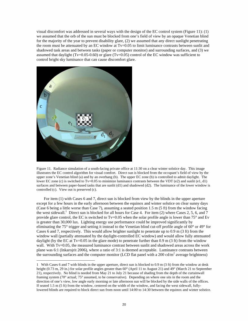
visual discomfort was addressed in several ways with the design of the EC control system (Figure 11): (1) we assumed that the orb of the sun must be blocked from one’s field of view by an opaque Venetian blind for the majority of the year to prevent disability glare, (2) we assumed that any direct sunlight penetrating the room must be attenuated by an EC window at Tv=0.05 to limit luminance contrasts between sunlit and shadowed task areas and between tasks (paper or computer monitor) and surrounding surfaces, and (3) we assumed that daylight (Tv=0.05-0.60) or glare (Tv=0.05) control of the EC window was sufficient to control bright sky luminance that can cause discomfort glare.

Figure 11. Radiance simulation of a south-facing private office at 11:30 on a clear winter solstice day. This image illustrates the EC control algorithm for visual comfort. Direct sun is blocked from the occupant’s field of view by the upper zone’s Venetian blind (a) and by an overhang (b). The upper EC zone (b) is controlled to admit daylight. The lower EC zone (c) is switched to Tv=0.05 to minimize luminance contrasts between the VDT (e2) and sunlit (e1, d1) surfaces and between paper-based tasks that are sunlit (d1) and shadowed (d2). The luminance of the lower window is controlled (c). View out is preserved (c).

For item (1) with Cases 6 and 7, direct sun is blocked from view by the blinds in the upper aperture

except for a few hours in the early afternoon between the equinox and winter solstice on clear sunny days (Case 6 being a little worse than Case 7), assuming a seated position 1.5 m (5 ft) from the window facing the west sidewall.1 Direct sun is blocked for all hours for Case 4. For item (2) where Cases 2, 5, 6, and 7 provide glare control, the EC is switched to Tv=0.05 when the solar profile angle is lower than 75° and Ev is greater than 30,000 lux. Lighting energy use performance could be improved significantly by eliminating the 75° trigger and setting it instead to the Venetian blind cut-off profile angle of 60° or 49° for Cases 6 and 7, respectively. This would allow brighter sunlight to penetrate up to 0.9 m (3 ft) from the window wall (partially attenuated by the daylight-controlled EC window) and would allow fully attenuated daylight (by the EC at Tv=0.05 in the glare mode) to penetrate further than 0.9 m (3 ft) from the window wall. With Tv=0.05, the measured luminance contrast between sunlit and shadowed areas across the work plane was 6:1 (Inkarojrit 2006), where a ratio of 3:1 is deemed acceptable. Luminance contrasts between the surrounding surfaces and the computer monitor (LCD flat panel with a 200 cd/m2 average brightness) 1 With Cases 6 and 7 with blinds in the upper aperture, direct sun is blocked to 0.9 m (3 ft) from the window at desk height (0.73 m, 29 in.) for solar profile angles greater than 60° (April 11 to August 21) and 49° (March 21 to September 21), respectively. No blind is needed from May 21 to July 21 because of shading from the depth of the curtainwall framing system (70° actual; 75° assumed, to be conservative). Depending on where one sits in the room and the direction of one’s view, low angle early morning or late afternoon sun will be blocked by the side walls of the offices. If seated 1.5 m (5 ft) from the window, centered on the width of the window, and facing the west sidewall, fully-lowered blinds are required to block direct sun from noon until 14:00 to 14:30 between the equinox and winter solstice.

a

b

c

d1d2

e1e2

a

b

c

d1d2

e1e2

21

were also found to be within acceptable ratios if Tv=0.05. For item (3), monitored average window luminance data for Cases 4, 6, and 7 over the year indicated that the EC window luminance exceeded 3000 cd/m2 for a maximum of 7 min per day (Clear 2006). The unshaded 1-zone glare mode (Cases 2 and 5) performed worse, exceeding 3000 cd/m2 for a maximum of 35 min per day for no more than 0.5% of the time. A window luminance exceeding 2000-5000 cd/m2 may cause discomfort glare depending on the task and view position (see Introduction regarding these thresholds). Modulating the EC transmittance proportionally to window luminance may also increase lighting energy use savings.

Due to the early stage of development of the integrated EC-lighting control system, visual comfort was not treated as a constraining requirement for the control of the reference and test cases in this field study. The resultant monitored visual comfort performance is documented in a separate report (Clear 2006). However, meeting visual comfort should be a requirement of the control algorithm; it must be addressed irrespective of energy-efficiency goals. One might conclude that meeting such criteria will result in insignificant energy savings, given the monitored results from this field study. Therefore, a Radiance-Mathematica daylight optimization study was performed where a 2-zone EC window system was first controlled to meet visual comfort requirements, then controlled to optimize for daylight (Fernandes et al. 2006). An interior Venetian blind was adjusted manually once per day based on visual comfort criteria for both the reference (Tv=0.60) and test cases. Annual lighting energy use savings were 48% (for the same room configuration as this monitored field study, given TMY climate data for Oakland, California) with significantly more hours of access to unobstructed view (view available for 98% versus 38% of the year). These optimized savings need to be verified in the field given the limitations of realistic sensor locations and controls.

5. Conclusions

A 20-month field study was conducted to measure the energy performance of south-facing large-area electrochromic (EC) windows with a broad switching range (Tv=0.60-0.05, SHGC=0.42-0.09) in a private office setting. Its performance was compared to a reference spectrally-selective low-e window (Tv=0.42, SHGC=0.22) with a fully retracted or lowered white Venetian blind. Both the reference and test cases had the same daylighting control system so as to isolate the energy savings to the EC window technology alone. Several EC window configurations were combined with different control algorithms and evaluated against the reference cases. Daily lighting energy use, daily cooling load due to solar heat gains, daily cooling load due to the window and lighting system, and peak cooling load due to solar heat gains were compared. These measured quantities were also related to exterior environmental variables. A net energy savings value was computed that combined the daily lighting energy use and cooling load data (assuming a COP of 3) to evaluate total energy savings impacts. Six of the seven test conditions evaluated spanned at least a six-month solstice-to-solstice period showing trends indicative of annual performance.

Monitored savings of an EC window controlled to maintain daylight work plane illuminance levels within a given range confirmed positive findings from earlier DOE-2 simulation studies. If the EC window is controlled to maximize daylight and energy-efficiency (Cases 1 and 3), average lighting energy savings were 6±7% and 26±15% compared to the reference case without and with fully lowered Venetian blinds (slat angle ~45°), respectively. Cooling load reductions in solar and lighting heat gains were 3±8% and 7±4%, respectively. For Case 3, daily net energy savings were 0.33-0.44 W/ft2-floor on days when the average incident vertical illuminance level (Ev) was less than 30,000 lux and 0.11-0.28 W/ft2-floor on days when Ev levels were greater than 30,000 lux. For this type of EC device, power used to switch and maintain the EC window at a steady-state can erode savings, but with a revised control circuit design and efficient power supply, EC power consumption levels are expected to be small.

If visual comfort requirements are addressed, a 2-zone EC window configuration (Case 7) with a shaded upper aperture (WWR=0.20) controlled for daylight and an unshaded lower aperture controlled for daylight and glare (WWR=0.30) provided mixed savings depending on solar conditions. Daily net energy savings of 0.11-0.56 W/ft2 were obtained for Ev levels less than 30,000 lux, but net energy use was increased by 0.11-0.39 W/ft2 for Ev levels greater than 30,000 lux. Average daily lighting energy savings over the year were 10±15% compared to the reference case with fully lowered Venetian blinds. Cooling load reductions were 0±3%. If the reference case had no daylighting controls, lighting energy savings would be 44±11%.

22

The field test data indicate that the average daily net energy savings resulting from EC windows are negligible if visual comfort requirements are met. However, the monitored results were dependent on the selected thresholds for glare and direct sun control. Lighting energy use savings varied by –50% to 50% depending on the control mode, threshold values, and solar conditions. Better tuned glare and direct sun control algorithms could be designed that would improve lighting energy performance. Further research is required to better understand how best to satisfy visual comfort criteria. We referenced a related simulation study to illustrate potential performance if visual comfort requirements are satisfied directly. This Radiance-Mathematica optimization study was performed for the same EC and room configuration as the field test where the visual comfort requirements were met and daylight illuminance was optimized. Annual lighting energy savings were estimated at 48% compared to a reference case with manually-operated Venetian blinds, indicating that glare control implemented for this field study may have been too severe. Separately, the field test and simulation results were also very dependent on how occupants operated the Venetian blind. Field studies indicate that shades are often operated infrequently (e.g., Rubins et al. 1978 found that blinds were adjusted more than once per day in only 50 out of 700 windows observed). More research is needed in both of these areas in order to obtain more realistic energy savings estimates for this emerging technology.

Peak demand reductions can be significant depending on how far the facility manager is willing to curtail load while inconveniencing the occupant. For a demand-response mode when blackouts are impending, the facility manager could shut the perimeter zone electric lights off (automated through the BMCS system) and set the EC windows to its maximum colored state. This would result in a reduction in peak cooling load due to the window of 19-26% maximum (clear sunny days) and 10-17% on average. Lighting peak reduction would depend on the lighting control system – if the reference case has the same dimming control system, then peak reductions would be zero. If the reference case has no occupancy sensors and no manual switches, then peak lighting demand reductions could be 100%. The occupant could turn on a 7-W LED task light, if needed, but with a 4.6-m- (15-ft) deep perimeter zone office and the likelihood that peak conditions will occur on a sunny day, daylight levels will probably be more than sufficient even with the Venetian blinds down.

Other observations were made when studying the data, confirming trends identified with simulation studies. If incident solar radiation levels are high and glare control is implemented (EC switches to its most colored state), lighting energy use savings decrease, while cooling load savings increase. If incident solar levels are low, lighting energy use savings increase, while cooling load savings decrease. For the former case, the EC uses its lower SHGC range (compared to the static reference case) to reduce window solar heat gains and garner cooling load savings. For the latter case, the EC uses its higher Tv range to garner lighting energy use savings over the static reference case. A broader EC switching range would therefore yield greater total energy savings across the range of solar conditions.

Finally, scatter in the data is explained in part by the inaccuracy of the EC window controller and the switching performance of the EC windows. Additional work is required to improve the accuracy of the EC intermediate switching controller so as to achieve more reliable and accurate results.

Non-energy benefits were not examined in this write-up. Results from the human factors subjective field study, visual comfort assessment, and Radiance-Mathematica study (performed as part of this project) indicate that EC windows provide significantly greater access to unobstructed views and are preferred over conventional static windows with an interior Venetian blind. These studies can be found on the project website: http://windows.lbl.gov/comm_perf/electroSys-cec.htm.

Acknowledgments

We would like to thank and acknowledge our LBNL colleagues for their contributions to this field test research: Duo Wang, Robert Clear, Howdy Goudey, Christian Kohler, Daniel Fuller, Steve Marsh, and Chuck Hambelton. We would also like to acknowledge in-kind contributions from Sage Electrochromics, Inc., Tom Mifflin at Wausau Window and Wall Systems and from LiteControl, Inc.

This work was supported by the California Energy Commission through its Public Interest Energy Research Program and by the Assistant Secretary for Energy Efficiency and Renewable Energy, Office of Building Technology, State and Community Programs, Office of Building Research and Standards of the U.S. Department of Energy under Contract No. DE-AC02-05CH11231.

23

References

Clear, R.D., V. Inkarojrit, E.S. Lee. 2005. Subject responses to electrochromic windows. Submitted to Energy and Buildings, February 23, 2005. LBNL-57125, Lawrence Berkeley National Laboratory, Berkeley, CA.

Clear, R.D. 2005. Assessment of visual comfort study in a full-scale electrochromic window testbed. Technical report. http://windows.lbl.gov/comm_perf/electroSys-cec.htm

Fernandes, L., G. Ward, E.S. Lee. 2005. Radiance-Mathematica optimization of electrochromic operations for occupant comfort and non-energy provisions. Technical report, http://windows.lbl.gov/comm_perf/electroSys-cec.htm.

Gugliermetti, F. and F. Bisegna. 2003. Visual and energy management of electrochromic windows in Mediterranean climates. Building and Environment 38(3):479-492.

Inkarojrit, V. 2004. Analysis of visual comfort using high-dynamic-range luminance images. Poster report. http://windows.lbl.gov/comm_perf/electroSys-cec.htm.

Karlsson, J. 2001. Control system and energy savings potential for switchable windows. Proceedings of the seventh International IBPSA Conference, Rio de Janeiro, Brazil, August 13-15, 2001.

Klems, J. 2004. Thermal calibration of the windows testbed facility. Technical report. http://windows.lbl.gov/comm_perf/electroSys-cec.htm

Lee, E.S., D. L. DiBartolomeo. 2002. "Application issues for large-area electrochromic windows in commercial buildings." Solar Energy Materials & Solar Cells 71 (2002) 465–491. LBNL Report 45841, Lawrence Berkeley National Laboratory, Berkeley, CA.

Lee, E.S., D.L. DiBartolomeo, S.E. Selkowitz. 2006. Daylighting control performance of a thin-film ceramic electrochromic window: field study results. Energy and Buildings 38 (2006): 30-44. LBNL-54924.

Platzer, W.J. 2003. Switchable façade technology – Energy efficient offices with smart facades. Proceedings of the ISES Solar World Congress 2003, Göteborg, Sweden, June 14-19, 2003. http://www.eu-swift.de/

Rubins, A.I., B.L. Collins, R.L. Tibbott. 1978. Window blinds as a potential energy saver - A case study (NBS Building Science Series 112). Washington, DC: U.S. Department of Commerce, National Bureau of Standards.

Sullivan, R., E.S. Lee, K. Papamichael, M. Rubin, S. Selkowitz. 1994. The effect of switching control strategies on the energy performance of electrochromic windows. Proceedings SPIE International Symposium on Optical Materials Technology for Energy Efficiency and Solar Energy Conversion XIII, April 18-22, 1994, Freiburg, Germany.

Wienold, J. 2003. Switchable façade technology: Building integration – Final report. Report number: swift-wp3-ise-jw-030616, Fraunhofer Institute for Solar Energy Systems, Heidenhofstr. 2, D-79110 Freiburg.