money and banking lecture notes lecture 1: introduction
TRANSCRIPT

MONEY AND BANKING LECTURE NOTES
Lecture 1: Introduction
➢ Key Initial Concepts:
➢ Nominal GDP; Real GDP; GDP Deflator (i.e. Nominal/Real); Calculating Growth
➢ Financial System Includes:
➢ Markets and Instruments traded in them
➢ Individuals and institutions trading in the markets
➢ Regulators and supervisors
➢ Main Function: Channeling funds from those who have excess to those who have deficit
➢ Market Participants:
➢ Borrowers: Firms (main); Households; Government; Foreigner (see Current Acc)
➢ Borrow for consumption & investment
➢ Lenders: Households (main); government; firms; foreigners
➢ What Do Lenders Worry About?
➢ The return they can receive
➢ Risk: default; income; inflation
➢ Liquidity
➢ What Do Borrowers Worry About?
➢ Returns they must pay
➢ Terms of the return: fixed interest debt is not state-contingent, while equity is!
➢ Length and flexibility of the borrowing (want to maximize maturity!)
➢ What is the Financial Account?
➢ One of the two main components of the balance of payments (along with current acc)
➢ Accounts for changes in the ownership of financial assets
➢ Usually, you look at the financial accounts of different sectors/countries over time
➢ Surplus in the Financial account money flowing into the country for financing a
current account deficit effectively represents borrowing
➢ Of course, all borrowing (deficit) must have an offsetting lending (surplus)
➢ How do matches between borrowers and lenders occur?
➢ Completely Direct
➢ Direct lending through an organized market (e.g. corporate bonds, equities)
➢ Through intermediation – no direct link between lenders & borrowers
➢ There are different ways of thinking about the organized markets
➢ Primary vs. Secondary markets
➢ OTC (negotiable terms) vs. Exchange markets
➢ Dealers (traders in particular assets) vs. brokers (match buyers and lenders)
➢ Money markets (SR) vs. Capital markets (LR)
➢ What is financial intermediation?
➢ Institutions which borrow funds from people who have saved in in turn make loans to
others (e.g. banks, pension funds, insurance companies); lots of benefits
➢ Reduced transaction costs
➢ Risk diversification
➢ Maturity transformation
➢ Reduces Asymmetric Information: Adverse Selection; Moral Hazard

➢ Two Main Types of Instruments
➢ Equity: ordinary shares; dividends; voting rights; price depends on S&D
➢ Bonds: fixed return; preferential debtor; no voting rights
➢ There is NO Single Interest Rate!
➢ Other Types of Instruments:
➢ Money Market: Treasury Bills; CDs; Commercial Paper; Repos; Eurodollars
➢ Capital Market: Stock; Mortgages; Corporate Bonds; Gov’t Bonds; Consumer Loans
➢ Financial services are highly regulated. Why?
➢ Need confidence of the public! The system NEEDS to be liquid
➢ Contagion
➢ Consumer protection…not caveat emptor
➢ But, there are problems due to regulation:
➢ Moral hazard
➢ Compliance costs
➢ Costs of entry & exit are high more monopoly power
➢ Bank Balance Sheets
Assets Liabilities
Reserves (@CB; fully liquid) Checkable Deposits (checking accounts)
Securities (varying liquidity) Time Deposits (savings accounts)
Loans Borrowings
Other Assets (physical capital) Bank Capital
➢ If the return earned on assets is more than what you pay on your liabilities profit!
➢ Bank capital is the residual that makes sure the Assets = Liabilities
➢ Reserves is made up of two components Required Reserved; Excess Reserves
➢ A T-Account Shows the Change in the Balance Sheet
➢ Suppose someone opens a bank account and $100 are deposited
➢ 10% RR ratio Bank has $90 of excess reserves. What does it do with them?
➢ One option is to create a new loan worth $90
➢ It has $90 of loans and $90 of new deposits.
➢ If the deposits stay in the bank, $81 of those are excess reserves!
➢ If the money leaves, deposits and reserves both decrease
➢ Alternatively, the bank could have bought securities worth $90 size of balance
sheet does not change here!
➢ Bank Management Includes the Following Concepts:
➢ Liquidity and reserve management
➢ Asset and liability management
➢ Capital adequacy – trade-off
➢ Capital prevents failures
➢ Capital lowers return to shareholders
➢ Credit risk and Interest rate management

➢ If the bank is low on liquid reserves, what can it do?
➢ Borrow from other banks (assets & liabilities increase)
➢ Borrow at the discount rate from the CB
➢ Try to recall loans and put the money into reserves
➢ Sell securities or physical capital to try and raise reserves
➢ Why might the financial system have macroeconomic effects?
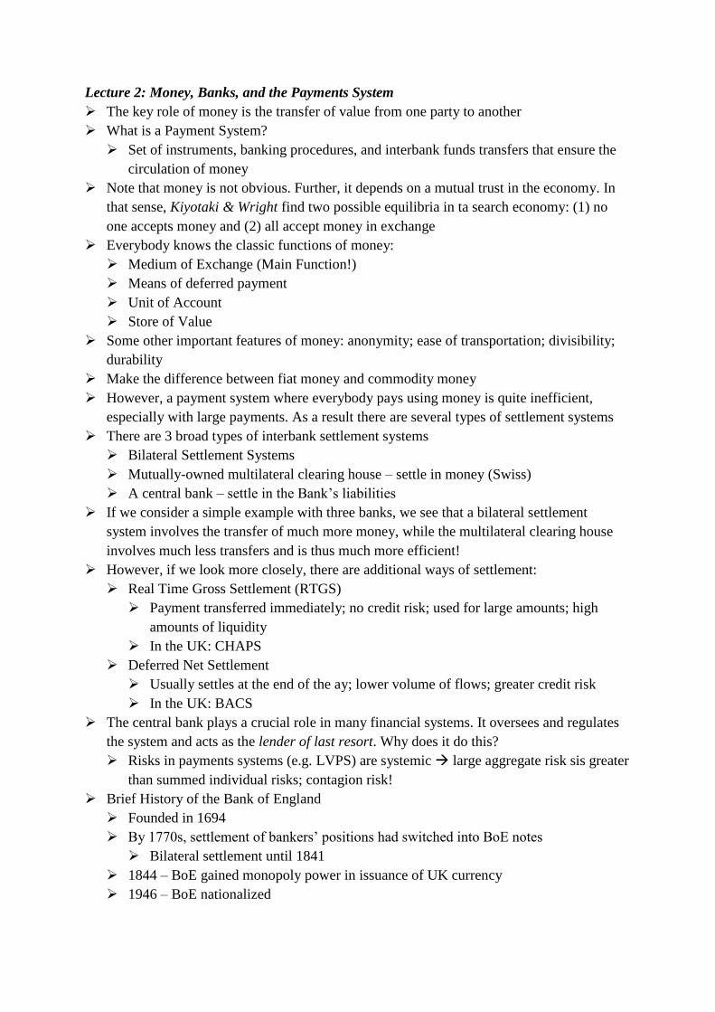
Lecture 2: Money, Banks, and the Payments System
➢ The key role of money is the transfer of value from one party to another
➢ What is a Payment System?
➢ Set of instruments, banking procedures, and interbank funds transfers that ensure the
circulation of money
➢ Note that money is not obvious. Further, it depends on a mutual trust in the economy. In
that sense, Kiyotaki & Wright find two possible equilibria in ta search economy: (1) no
one accepts money and (2) all accept money in exchange
➢ Everybody knows the classic functions of money:
➢ Medium of Exchange (Main Function!)
➢ Means of deferred payment
➢ Unit of Account
➢ Store of Value
➢ Some other important features of money: anonymity; ease of transportation; divisibility;
durability
➢ Make the difference between fiat money and commodity money
➢ However, a payment system where everybody pays using money is quite inefficient,
especially with large payments. As a result there are several types of settlement systems
➢ There are 3 broad types of interbank settlement systems
➢ Bilateral Settlement Systems
➢ Mutually-owned multilateral clearing house – settle in money (Swiss)
➢ A central bank – settle in the Bank’s liabilities
➢ If we consider a simple example with three banks, we see that a bilateral settlement
system involves the transfer of much more money, while the multilateral clearing house
involves much less transfers and is thus much more efficient!
➢ However, if we look more closely, there are additional ways of settlement:
➢ Real Time Gross Settlement (RTGS)
➢ Payment transferred immediately; no credit risk; used for large amounts; high
amounts of liquidity
➢ In the UK: CHAPS
➢ Deferred Net Settlement
➢ Usually settles at the end of the ay; lower volume of flows; greater credit risk
➢ In the UK: BACS
➢ The central bank plays a crucial role in many financial systems. It oversees and regulates
the system and acts as the lender of last resort. Why does it do this?
➢ Risks in payments systems (e.g. LVPS) are systemic large aggregate risk sis greater
than summed individual risks; contagion risk!
➢ Brief History of the Bank of England
➢ Founded in 1694
➢ By 1770s, settlement of bankers’ positions had switched into BoE notes
➢ Bilateral settlement until 1841
➢ 1844 – BoE gained monopoly power in issuance of UK currency
➢ 1946 – BoE nationalized

➢ Recent (non-crisis) Policy Issues
➢ How and on what terms should a CB supply money to financial institutions?
➢ What is the future for money? BitCoin?
Measuring Money
➢ Money is very difficult to measure; there is infrequent reporting, different definitions
(broad/narrow) and seasonal adjustments
➢ Generally speaking, the money supply is the total quantity of money available
➢ In the US, the two measures are:
➢ M1: Currency in circulation + checking accounts (currency)
➢ M2: M1 + Savings Accounts + Small Time Deposits (broad money)
➢ How does money enter the system?
➢ The CB prints money, buys securities, or lends it to commercial banks.
➢ In the UK, there are two main measures of money:
➢ M0: Sterling notes and coin outside BoE + Banks’ operational deposits in BoE
➢ This is the Monetary Base (i.e. Reserves + Cash)
➢ Since 2006, this has been discontinued and narrow money = “Notes and Coins”
➢ M4: The M4 private sector’s holdings of:
➢ Notes & coin; sterling deposits; CDs; CP; claims on UK MFIs; estimated holdings
of sterling bank bills;
➢ M4PS refers to the UK private sector other than MFIs
➢ Don’t treat each of the different assets as perfect substitutes!
➢ As we saw previously, a typical bank balance sheet looks like this:
Assets Liabilities
Reserves (@CB; fully liquid) 4% Checkable Deposits (checking accounts) 7%
Securities (varying liquidity) 23% Time Deposits (savings accounts) 59%
Loans 66% Borrowings 26%
Other Assets (physical capital) 7% Bank Capital 8%
➢ The key idea is to make more money on assets than you pay on liabilities!
➢ On the other hand, the Central Bank Balance sheet looks like this:
Assets Liabilities
Gov’t Securities (varying liquidity) Currency in Circulation
Discount Loans to Banks Reserves (from Banks)
Other Assets
➢ The liabilities of the CB is known as the Monetary Base (MB)
➢ The CB can engage in OMOs to change the monetary base!
➢ By changing the monetary base, the central bank can create money!

➢ The CB can use a relatively small OMO to create a large increase in the money supply.
This process works through multiple deposit creation across banks!
➢ In effect, if each Bank leverages up on the basis of only 10% of new deposits being
kept as required reserves, the overall effect will be:
Re ( )( )
Re Re
serves InitialDeposits D
serve quirement
➢ An OMO of $100 can increase deposits by $1000!
➢ A more formal way to see this is by examining the Money Multiplier Model:
( )
Re
Re
; ;
Re
1
11
s
S
S
M Cash Deposits D
MB Cash serves
serves RR ER
ER RR Cashe r c
D D D
MB Cash serves Cash ER RR
MBc e r
D
MB c e r D
M Cash D c D D c D
MB cM c MB m MB
c e r c e r
➢ As long as 𝑟 + 𝑒 < 1, an increase in MB that goes into currency is not multiplies, and
therefore higher c means lower multiplier
➢ Similarly, higher e and higher r lower the multiplier
➢ Some approximate values are: 𝑒 ≈ 0.001 − 0.003; 𝑟 ≈ 0.1; 𝑐 ≈ 0.5
➢ Although this is a simple and intuitive approach to understanding how money creation
works, it is unrealistic and nobody really follows it! Why?
➢ Quantity controls excessive volatility in prices
➢ Predicting CB liabilities no always accurate
➢ Bank assets are non-marketable
➢ Banks are more likely to be constrained by equity rather than by reserve requirements
➢ Central banks can influence the total amount of money by controlling IRs!
The Subprime and Financial Crisis
➢ A big takeaway from looking at the crisis is that bank losses due to bad mortgages were
relatively small (around 3% of stock market).
➢ We need to understand how the shock from the subprime housing crisis got transmitted to
become the large scale, global crisis that we have seen in the last years!
➢ A key idea to understanding this is leverage:
AssetsLeverage
Capital

➢ If we hold debt constant, leverage is inversely proportional to asset values
➢ Asset value falls leverage increases leverage is counter-cyclical!
➢ This is what we see with households
➢ HOWEVER, when we look at banks we see pro-cyclical leverage
➢ As asset prices go up, banks increase leverage by buying even more assets using debt
➢ Buying more assets pushes up the value of assets virtuous (or vicious) cycle
➢ When prices start to fall, we get a firesale of assets!
➢ Alternatively, banks could raise capital and use the proceeds to buy assets in order to
decrease their leverage….but, who is going to buy?
➢ In the beginning of the crisis, banks tried to cover the declines in the values of their assets
by raising new capital
➢ However, from September 2008, banks were unable to raise new capital, so the
government stepped in to recapitalize the banks and stop the firesales
➢ Huge jump in the interbank market rate!!!
➢ Confidence was gone!
➢ How was this different from the Northern Rock crisis? What were the primary
failings of the bank? What was the policymakers’ response?

Lecture 3: Risk, Bonds, and the Determination of Interest Rates
➢ This comes up every year in the exam!
➢ The basic idea is that there is some “price” for time:
➢ Money today is worth more than money tomorrow because, if nothing else, you could
put it in a bank and earn interest.
➢ Present Value:
➢ The present value of a stream of money is the amount that they are worth today
1 2
0 2...
1 1 1
N
N
xx xPV x
r r r
➢ In the above, r is the discount factor (e.g. interest rate)
➢ This concept is used for the pricing of most assets, such as bonds and equities
➢ Bond Market:
➢ A financial market where participants buy and sell debt securities in the form of bonds
➢ Also known as debt, credit, fixed income market
➢ It is large and important in modern economies!
➢ Basic characteristics of bonds:
➢ Fixed Return: Per period interest; Principal at maturity date
➢ Preferential debtor; no voting rights
➢ Coupon bonds vs. Discount bonds (no coupon); Perpetuity/Consols
➢ The closest measure of the interest rate for bonds is the yield to maturity:
➢ The interest rate that equates the present value of cash flow payments from a debt
instrument with its value today
➢ Prices and yields are inversely related
➢ The yield is conceptually different from the “return”, which takes into account the
selling price as a % of the purchase price!
➢ A fixed interest bond with coupons, c, and a final payment, M has a valuation of:
0
1 1 1
Nt
t Nt
c MP
i i
➢ Where t is the period between coupon payments and i is the YTM
➢ The inverse relationship is obvious. Every time S&D forces change the price of the
bond, the YTM must adjust
➢ There is a number of other pricings we need to consider:
1. Valuing the coupon part separately:
0
11
1N
annuityi
P ci
2. Valuing a zero-coupon bond
0
1
zero coupon
N
MP
i
3. Aside the final price of the annuity can be worked out from:
0 1N
NP P i

4. Dirrrty price – adds in the value of accrued interest
0
1
#days since last coupon
# days in each coupon period1 1
Nt
t Nt
c MP c
i i
5. Ex-Dividend Price more complicated to calculate dirty price
6. A pure annuity 𝑁 = ∞
0
pure annuity cP
i
7. Effective annual rate takes into account compounding
1 1F
r i
➢ F – number of coupon payments per year
➢ i – periodic interest rate is the annual interest rate, R, divided by F
➢ On top of this there are some further complications in the calculating of bond prices:
➢ Simple Yield to Maturity
➢ Holding Period Yield Assumes you don’t hold the bon to maturity and that the
coupons are reinvested at different rates
➢ Real vs. Nominal Interest Rates Fisher Equation ei r
➢ However we usually allow from some risk and liquidity premia: ei r risk liquidity
➢ In terms of pricing, bonds are traded in organized markets and so their prices (and yields)
depend on supply and demand factors:
➢ Demand: Wealth (+); Coupons (+); Expected inflation (-); Risk (-); Liquidity (+)
➢ Supply: Expected profitability (+); Expected inflation (+); Government budget deficit
increase (+)
➢ What happens to yields as a result of the business cycle? It is ambiguous!
➢ A Simple Representative Investor Model can shed light on IR Determination
➢ The premise is a two-period consumption optimization in which the investor has some
exogenous endowment in each period and bond holdings (yielding interest) provide
the link between the two periods
0 1
0 1 1 2
1 2 1 0
0 2 1 0
1 0
0
1 1 0 0
1 0
max , exp
subject to: 1
1
exp exp 1
10 1 exp
In equilibrium: C and
1exp 1
u C u C u C C
C y b C y r b
C y r y C
U C C y r y C
U Cr C C
C
y C y
r y y
➢ Higher future endowment lower demand for savings higher IR
➢ Higher patience more demand for savings lower IR, higher 𝜌

➢ We have seen two theories of IR determination so far: the Loanable funds (with S&D) and
the Representative Investor Model.
➢ Another theory of IR determination is the Liquidity Preference Approach KEYNES
➢ Combines thinking about money and bond markets
➢ Starts with the assumption that Money and Bond Supply = Money and Bond Demand
MS BS MD BD
MS MD BD BS
➢ Keynes claimed that thinking about money equilibrium is equivalent to thinking about
bond market equilibrium!
➢ If there is excess supply in the money market, there must be an excess of demand in
the bond market money IRs will fall, bond IRs will rise
➢ Keynes’ Idea: Interest rate is the reward for giving up liquidity. Liquidity Effect:
Higher MS lower IRs
➢ This is good, as long as we hold inflation constant! When we add (expected) inflation to
the mix, the overall effect of MS changes become very ambiguous indeed!
➢ In reality, the CB announces the short term interest rate and then engineers it in the
Bank lending market
➢ Although the CB controls 1 very short rate, it is usually LR rates that matter more for
economic decisions the relation between SR and LR is crucial!
➢ With that, we go into the discussion of the Term Structure of Interest Rates!
➢ Term Structure of Interest Rates:
➢ Refers to the patter of interest rates available on assets differentiated solely on their
term of maturity.
➢ Several Key facts about the term structure are:
1. Interest rates of different maturities tend to move together!
2. Yield curve slopes up if IRs are historically low, or vice versa
3. LR yields to be higher than SR yields key point we need to examine!
➢ There are several sub-theories here:
1. (Pure) Expectations Theory
➢ The idea is that we should be indifferent between taking out a two year bond and
taking a 1 year bond, and reinvesting it after one year at the future IRs
2
01 12 021 1 1i i i
➢ Here, 𝑖12 is the forward rate – implied future spot rate!
➢ In general, we can approximate. We can say that the LR yield should be
approximately the average of the short term yields
01 12 ( 1)
0
... T T
T
i i ii
T
➢ This theory can explain facts 1 and 2, but not fact 3. Also, Mankiw & Miron
(1986) show that there is little evidence that term structure predicts future interest
rates!
2. Segmented Markets Theory
➢ Markets for SR and LR securities are separate and there is no relationship
➢ However, this violates point 3 directly overall, it is a little rubbish

3. Liquidity Premium Theory
01 12 ( 1)
0
... T T T
T L
i i ii
T
➢ This is basically the Expectations theory plus a liquidity premium (or risk
premium) for a security of maturity T
➢ Digression: Bonds are Risky and there are different types of risk involved. These
naturally affect the premium required on long-term securities
➢ Default Risk; Liquidity Risk; Reinvestment & Capital Risk; Inflation Risk; Tax
Consideration
➢ For example, credit agencies exist which assess the credit worthiness of bond-
issuers; higher rating higher bond price lower yield required
4. Preferred Habitat Theory
➢ This is similar to the liquidity premium theory
➢ Investors have a preferred maturity (habitat)
➢ Other bonds must offer a sufficient premium to induce these investors away from
their preferred maturities
➢ NB: Interpreting the Yield Curve will depend on which theory of IR determination you
subscribe to!

Lecture 4: Equities
➢ Basic features of the equity market:
➢ Shares, stocks, and equities are commonly used to describe “ordinary shares”
➢ Shareholders may get an annual share of profits (earnings) as dividend; own part of the
company; have voting rights;
➢ Price of shares varies based on supply and demand
➢ This is all related to the equity part of the balance sheet
➢ In the UK, the face value of shares may be £1, 50p, or down to 1p. But, this does not
matter. The share price depends on the supply and demand!
➢ Some companies are privately owned – no shares
➢ But, if a company goes public and decides to “float”, its shares become traded in an
organized exchange market (e.g. London Stock Exchange)
➢ Initial Public Offering (IPO)
➢ Increases sources of eternal finance; may improve image; increases extent of
regulatory disclosure; increases liquidity of assets!
➢ Some IPO facts:
➢ Usually underwritten by an investment bank
➢ IPO shares are generally underpriced and often jump when trading begins
➢ The public is general excluded from this initial process
➢ Apart from these “ordinary shares” other types of shares also exist:
➢ Deferred ordinary shared
➢ Preference Shares
➢ Dual class stock
➢ Golden shares
➢ Of course, the extent of equity investment differs across countries. Two general trends can
be seen however:
➢ Growth of stock market capitalization as a % of GDP from 1990-2008
➢ Huge fall in capitalization as a result of the crisis!
➢ It is difficult to follow trends in equities when there are so many of them. For that reason,
there are overall share indices relating to firms on an exchange:
➢ FTSE 100, FTSE250, FTSE350; Dow Jones; S&P 500; DAX; CAC 40
t it it
i
Index w price
➢ These indices can be:
➢ Price weighted (Dow Jones)
➢ Market capitalization weighted (FTSE)
➢ Now, we turn to the most interesting and most difficult part of equities: pricing
➢ The returns we get from an equity can simply be discounted over time, as we have
seen with bond pricing:
1 2
0 2...
1 1 1 1
N N
N N
e e e e
D PD DP
k k k k
➢ 𝑘𝑒 is the required return on capital; D are the dividends; 𝑃𝑁 is the price when sold
➢ The reason shares trade so much is varying beliefs about D, k, 𝑃𝑁
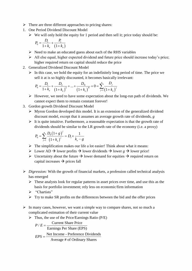
➢ There are three different approaches to pricing shares:
1. One Period Dividend Discount Model
➢ We will only hold the equity for 1 period and then sell it; price today should be:
1 1
01 1e e
D PP
k k
➢ Need to make an educated guess about each of the RHS variables
➢ All else equal, higher expected dividend and future price should increase today’s price;
higher required return on capital should reduce the price
2. Generalized Dividend Discount Model
➢ In this case, we hold the equity for an indefinitely long period of time. The price we
sell it at is so highly discounted, it becomes basically irrelevant:
1 2
0 21
... 01 1 1 1
njN
N jje e e e
DDD DP
k k k k
➢ However, we need to have some expectation about the long-run path of dividends. We
cannot expect them to remain constant forever!
3. Gordon growth Dividend Discount Model
➢ Myron Gordon developed this model. It is an extension of the generalized dividend
discount model, except that it assumes an average growth rate of dividends, g
➢ It is quite intuitive. Furthermore, a reasonable expectation is that the growth rate of
dividends should be similar to the LR growth rate of the economy (i.e. a proxy)
0
0 1
1
1 1
1
jn
jj ee
D gP D
k gk
➢ The simplification makes our life a lot easier! Think about what it means:
➢ Lower AD lower profits lower dividends lower g lower price!
➢ Uncertainty about the future lower demand for equities required return on
capital increases prices fall
➢ Digression: With the growth of financial markets, a profession called technical analysis
has emerged
➢ These analysts look for regular patterns in asset prices over time, and use this as the
basis for portfolio investment; rely less on economic/firm information
➢ “Chartists”
➢ Try to make SR profits on the differences between the bid and the offer prices
➢ In many cases, however, we want a simple way to compare shares, not so much a
complicated estimation of their current value
➢ Thus, the use of the Price/Earnings Ratio (P/E)
Current Share Price/
Earnings Per Share (EPS)
Net Income - Preference Dividends
Average # of Ordinary Shares
P E
EPS

➢ High P/E Market must be expecting higher earnings in the future relative to now!
➢ Higher earnings growth relative to lower P/E companies
➢ Be Careful: P/E is an accounting measure and can be manipulated
➢ Furthermore, you cannot reasonable compare P/E ratios across industries
Rational Expectations and Efficient Markets Hypothesis
➢ Rational Expectations:
➢ Forecasts made by agents use all available current information and are ex-ante
correct! It does not mean they will be ex-post correct!
OPE X X
➢ Any forecast errors should on average be zero!
➢ This hypothesis is very useful in economics and has had a profound impact on the
field, but it does have limitations:
➢ It is costly to process all available information!
➢ Some information is hard to find so forecasts may not be optimal!
➢ The Efficient markets Hypothesis (see Fama) is that:
➢ Current price of a financial asset should reflect all available information & optimal
forecast
➢ There should be no exploitable profit-making opportunities
➢ If you outperform the market, your strategy was mostly luck!
➢ Evidence in Favor of EMH:
➢ Investment analysts rarely do consistently well from year to year
➢ Best guess of future price is today’s price (unit root; Random Walk)
➢ Technical analysts don’t outperform the market on average!
➢ Some evidence against EMH:
➢ Relies on rationality of at least a few large investors
➢ News events are often slow to be reflected in price information
➢ Is the implication that bubbles are also rational?
➢ On average, share prices tend to be more volatile than dividends ex-post (Shiller)
➢ There is a field called Behavioral Finance which studies the influence of psychology on
the behavior of financial practitioners and the subsequent effect on markets
➢ Helps explain why and how markets might be inefficient
➢ Consider Keynes’ Beauty Contest
➢ Some relevant concepts: Loss aversion; Social contagion; over-confidence!

Lecture 5: Financial Derivatives
➢ Difference between a long position (net assets) and a short position (net liabilities)
➢ If you are long, then you would profit (lose) if asset prices increase (decrease)
➢ If you are short, you would profit (lose) if asset prices decrease (increase)
➢ Hedging Risk:
➢ Involves engaging in a financial transaction which offsets you current long (short)
position by taking a equivalent short (long) position!
➢ Four similar but distinct instruments to hedge are:
➢ Forwards
➢ Futures
➢ Options
➢ Swaps
➢ Forward:
➢ A contract between parties to carry out a predetermined financial transaction as some
predetermined (forward) time
➢ Advantage: flexibility;
➢ Issues: need to find a suitable counterparty (liquidity risk); default risk
➢ Financial Futures:
➢ A contract to buy or sell a standardized amount (per contract) of a particular defined
asset at a predefined point in the future
➢ Large futures market for US Treasury bonds at the Chicago Board of Trade (CBOT)
➢ Example: A $100K Treasury bond’s futures price is 118 point (meaning $118)
➢ Price at expiration is 110 if you are selling the contract 8 point profit
➢ If you have to take delivery (buy) the asset you are making a 8 point loss!
➢ Example: Bank holds Treasury bonds (it is long in bonds)
➢ It is worried it might lose if the value of these bonds fell (IRs increased)
➢ It could hedge by selling futures contracts at today’s futures price (becomes short)
➢ This way, if the asset value does fall the futures contract will make money!
➢ Losses or gains are linear in settlement price
➢ You can settle by taking an offsetting position with another futures contract. The
underlying asset rarely changes hands
➢ Options
➢ Financial contracts to allow one party to decide whether or not to engage in a
transaction (buy or sell) at a predetermined strike price on (or up to) a specified date
➢ Usually on futures contracts rather than actual assets
➢ Two Types: Call Option; Put Option
➢ Also, distinguish between European options and American options
➢ Pricing is very complicated Black-Scholes pricing
➢ Market makers take the other side of options for a premium (fee)
➢ Example: You pay $4K for a call option at a strike price of 118 in 1 month you
have the right to buy the bond for 118
➢ If the price is 110 (out of money), you don’t buy; if the price is 120 (in the money)
you buy but have a net loss of 2; if it is 118 (at the money), loss of 4
➢ The opposite is true for put options!

➢ Swaps:
➢ Swaps involve an agreement to exchange the payments from an asset (leg) between
two parties (rather than the assets themselves)
➢ E.g. Interest rate swaps can be used to hedge interest rate risks
➢ Problems: a lack of liquidity and default risk!
➢ There are many different kinds of credit derivatives:
➢ Credit options buy an option on the spread between Libor and Baa bonds which, for
a premium, protects against adverse movements in the rates
➢ Credit Default Swaps – a form of insurance you pay a premium that means that if
the company gets downgraded, goes bankrupt or defaults on its debt, you get a certain
payment

Lecture 6: Inflation and Business Cycles
➢ Inflation: a sustained general rise in the price level in the economy
➢ Measured using: CPI; PPI; Deflators
➢ If prices and wages are rising, what are the disadvantages of this?
➢ Makes it difficult to detect relative price changes
➢ High inflation volatile inflation Uncertainty!
➢ Very high inflation undermines the role of money as a store of value!
➢ Shoe leather costs; menu costs
➢ Interaction with tax system (usually in nominal terms)
➢ (Arbitrary) redistribution effects!
➢ Nominal contracts break down; long-term contracts avoided
➢ Overall, high inflation can create very big problems for the economy
➢ Some historical trends in inflation:
➢ Pre 1900s: commodity money cannot really have very rapid inflation
➢ Post 1900s: switch to “fiat” money” Gov’t involves in some very sketchy activities,
printing money, hyperinflations, etc.
➢ Post 1980s: Government abuse of fiat money leads to independent central banks!
A Quantity Theory of Money
➢ Friedman: “Inflation is always and everywhere a monetary phenomenon”
➢ The Quantity Theory is very closely related to the equation of exchange:
M V P Y
➢ If we assume the V is relatively constant, the quantity theory tell us that increases in
money supply will increase nominal GDP
➢ But, will it increase real GDP or will it increase the price level?
➢ The gist of the Quantity Theory is that monetary expansion may have real effects in the
short-run, but in the long run, it only affects inflation (money neutrality)
➢ LR data provide substantial support for the quantity theory. However, the same cannot be
said for SR data low correlation between money supply growth and inflation!
➢ Conclusion:
➢ MP needs to take a more sophisticated approach to controlling inflation than simply
controlling the money supply, particularly in the SR and medium-run
The Romer (IS-MP) Model
➢ IS Curve is the same as in the IS-LM Model derived from Keynesian Cross
➢ MP Curve is an upward sloping curve in (Y;r) space reflects the fact that when output
rises or inflation rises, the CB will increase the real interest rate
➢ Monetary policy affects RIRs via the equilibrium of the real money supply and real money
demand:
,e
M Y YL i Y
P V i V r
➢ If prices are fully flexible, money is neutral; if prices are fully fixed or adjust slowly,
an increase in M must be matched by higher Y and lower RIR (i.e. higher V)

The Romer (AD-IA) Model
➢ With the AD-IA Model, we can think about the process for inflation and how monetary
authorities will respond
➢ NB: At any point in time, inflation is given! IA Curve must be HORIZONTAL
➢ When output is above the natural rate, inflation rises. When it is below, inflation falls.
When output equals the natural rate, inflation is constant
➢ And AD shock increases inflationary pressures leads to inflation rising
➢ Inflation shock lowers output since it will lead to higher RIRs
➢ Analyze both effects of Fiscal Policy and Monetary Policy within the IS-MP and AD-IA
frameworks! These both influence aggregate demand!
➢ On the other hand, there are two aggregate supply shocks in this model:
➢ Inflation shocks disturbance to the usual inflation rate that shifts the IA line
➢ Supply Shocks changes in the natural rate of output
Inflation and Government Deficit
=
Deficit G T
B M
➢ If the government does not increase taxation or borrow from the private sector (B), then
deficit spending must be paid for by either:
➢ New Money Printed
➢ New bonds that the public will not hold CB conducts OMOs Increases M
➢ A potential disastrous result is hyperinflation. This results from very rapid increases in the
money supply…always result from the printing of money to finance a budget deficit
➢ Hyperinflation dynamics lead to a vicious cycle:
➢ Government deficit financed by printing money
➢ Increase in case increases prices directly
➢ Value of money declines increases inflation further
➢ Lax in tax collection mean that real gov’t revenue falls
➢ Increases the deficit back to step 1
➢ How do you stop a hyperinflation:
➢ Gov’t needs to reinstate the public’s belief in the value of money. Credibility!
➢ Money supply growth needs to be lowered!
➢ Government budget deficit stabilization FISCAL REFORM!
Business Cycles
➢ These are short term phenomena made up of expansions and contractions. During the
expansions, economic indicators increase. During contractions, they fall
➢ Key terms here are: expansion; peak; contraction (recession); trough
➢ What exactly is a recession:
➢ 2 quarters of falling GDP? Very poor definition.
➢ NBER Business Cycle Dating Committee – evaluate a range of indicators to determine
beginnings and ends of contractions
➢ Statistical tools can “identify” business cycles as deviations from trend

➢ The Hodrick-Prescott filter is one filter for extracting the cyclical component from raw
macroeconomic time series
➢ An appropriate smoothness parameter for quarterly data is 1600; for annual data is
100, and for monthly data is 14,400
➢ Some general features of business cycles
➢ NOT Regular do not behave in some consistent manner do not rely on some
underlying component
➢ Expansions tend to be long and mild
➢ Recessions tend to be short but more dramatic
➢ Business cycles usually have a duration of 4-10 years
➢ A similar, but distinct concept is the output gap
➢ This measures the difference between actual activity and potential activity
➢ Although it is more useful, it is much harder to estimate. One way is through the
production function technique
➢ Finally, a key concept in the study of business cycles is making a distinction between the
initial shock to the economy (impulse) and the mechanism that transmits shocks over time
(propagation mechanism)
➢ It is this latter effect which makes business cycles powerful and persistent
Monetary Policy
➢ Monetary policy is very powerful in the SR because IRs have substantial impacts on
aggregate demand, though affecting decisions of consumers and firms
➢ However, Monetary Policy is very difficult. Some of the complications are:
➢ “Long and variable lags” faced by MP actions
➢ Very hard to tell if whether the MP stance is too loose, too tight, or just right
➢ Not always clear if the BC is driven by demand or supply shocks!
➢ Getting it wrong could have bad effects (e.g. stagflation)
➢ The Monetary Transmission Mechanism refers to how MP changes on SR IRs affect
real variables and ultimately inflation!
➢ Starting at the end, we define the CPI as:
,
0
% %N
t i i t
i
CPI w p
➢ Where w refers to the weight of the ith good in the basket and %change in p refers to
the change in prices of the said good
➢ Inflationary Pressures are Intimately Related to the output gap
➢ Positive output gap demand is greater than potential output upward pressure on
prices
➢ However, determining the level of demand relative to potential supply is not as easy as
it sounds! Need to care about economic growth, because that determines inflation
➢ How does monetary policy affect AD?
( )AD C I G X M
➢ In general, MP does not have big effects on G

➢ As for the other three components of AD, the effect of MP will depend on how the
change in SR IRs will affect:
➢ Market Interest Rates
➢ Asset Prices
➢ The exchange rate
➢ The expectations for the future development of each of these!
➢ When there is a shock in int’l markets, how does the CB respond?
➢ It can do nothing about the 1st round effects
➢ However, the CBs can deal with the second round effects!
➢ Finally, since the 1990s, monetary policy in developed countries has become anchored by
the actions and credibility of independent central banks
➢ Inflation has been low and under control
➢ Inflation expectations have been under control
➢ As a result, temporary changes in inflation do not translate into wage and price
decisions of workers and firms! Stability is ensured!
➢ This development followed from the research of Kydland & Prescott, and Barro &
Gordon developed the time inconsistency problem of discretionary policymakers
➢ The 1980s are iconic for Paul Volcker’s disinflationary policies which, although they
generated a severe recession in the SR, managed to reduce inflation, and the economy
recovered afterwards!

Lecture 7: Monetary Policy Frameworks
➢ There are two possible ways to achieve central bank credibility
➢ Central bank independence constrained discretion; remove the incentive for time
inconsistency; this is most modern monetary institutions
➢ Removes inflation bias inherent in democratic politics!
➢ Conduct policy through an explicit framework
➢ How do we define independency? Not so simple.
➢ Goal independence
➢ Operational independence
➢ No deficit finance; communication without constraint; independence from political
bodies in general, etc.
➢ The famous “Alesina & Summers” Chart negative correlation between average
inflation and index of CB independence
➢ In order to make MP more transparent, independent CBs will generally try to achieve a
certain objective:
➢ Exchange rate targeting
➢ Monetary targets
➢ Inflation Targets
Inflation Targeting
➢ Independent CB announces a policy of keeping the inflation close to some LR target
➢ E.g. New Zealand; Canada; UK; Sweden; Finland; Australia
➢ Benefits:
➢ Simple and easily understood
➢ Removes some uncertainty about direction of policy
➢ Does not imply CBs will care only about inflation! They consider all indicators
➢ Ok, an inflation target. So what should this target rate be?
➢ Zero? Perfect price stability.
➢ Negative? Friedman
➢ Reality: low and stable positive inflation
➢ It is important to note the difference between inflation targeting and price level targeting
➢ With the latter, we cannot ignore past deviations
➢ If the price level was below the target for some time, this will have to be met by a
period of above target inflation
➢ Over the long run, the two should not be too different!
Conduct of Monetary Policy
➢ We cannot go far in the context of CB operation without getting to the Taylor Rule:
* *1.5 0.5t tNIR R y y
➢ The weights assigned to inflation and output deviations, of course, depend on the
particular CB mandate
➢ Although this rule does a good job at summarizing CB functions, it is imperative to
understand that no central bank follows an explicit Taylor rule!

➢ The Bank of England is one example of an inflation targeter
➢ The target, of course is (2%±1%)
➢ However, in line with its mandate, the BoE must also support the gov’t objectives for
growth and employment! It must be sensible
➢ Furthermore, the Bank has operational independence, but not goal independence!
➢ Key components of the BoE’s monetary policy determination:
➢ 9-member Monetary Policy Committee
➢ IR decisions made on a monthly base with a majority vote
➢ Of course, the BoE really tries to target the inflation in 1.5-2 years’ time, by
considering both inflation and output outlooks
➢ See article on the conduct of monetary policy in the United Kingdom
➢ Every quarter, the MPC agrees on a forecast for inflation and produce “fancharts” for
GDP growth and inflation
➢ A good summary of Monetary policy at the ECB, Fed, BoE
Quantitative Easing
➢ Since March 2009, the BoE has left NIRs at 0.5% (essentially ZLB) and now does QE
➢ The weak money means that too little money will circulate
➢ BoE directly buys assets from the market!
➢ Asset sellers have more money to spend or buy other assets
➢ Should lower yields cost of borrowing for businesses lowered
➢ Banks have more reserves so they start to lend more (bank lending channel)
➢ NB: At the ZLB, falling rates of expected inflation increase the real interest rate!
➢ The theory is that of the Zero Lower Bound by Romer!
➢ IS curve has a kink inwards below the optimal output level!
➢ IA can no longer adjust in order to bring output back to natural level
➢ How do you avoid a liquidity trap?
➢ Huge fiscal policy action needed! Shift the IS curve back out!
➢ Generate inflation expectations (e.g. using QE)?

➢ “It’s like we’ve used Super Glue on inflation expectations and now we want to raise them,
and we don’t know how!”
➢ On top of this, the BoE also cannot let inflation get out of control. Consequently, it needs
a good exit strategy for when the markets and the economy has recovered
➢ For a while, this exit strategy was called Forward Guidance
➢ MPC intended to keep the Bank rate fixed until unemployment fell below 5%
➢ However, this is now outdated
➢ Now, there is no explicit exit strategy!
➢ An important question is: Is QE Inflationary? Well, what happened to monetary
aggregates?
➢ The monetary base M0 increased dramatically with QE1 and the QE2
➢ However, M1 has only increased slightly over time! Why?
➢ The money multiplier collapsed with the start of QE. Although banks had a lot more
reserves, their reserve ratio increased dramatically
➢ Banks had the reserves, but were not lending them!
➢ As for the C/D ratio, it did not change much. Contrast this with the case of the Great
Depression!
➢ In these circumstances, there is only so much a central bank can do.
Financial Stability
➢ What does a stable financial system need to insure?
➢ Consumer/Firm confidence
➢ Provide critical services
➢ Prevent contagion of idiosyncratic problems
➢ The BoE has the objective to “contribute to protecting and enhancing the stability of the
financial systems of the United Kingdom”
➢ Risk assessment, market intelligence, payments systems oversight, banking and
market operations, lender of last resort, dealing with distressed banks
➢ Bank of England of 1998 was amended in 2012 sets out the objectives of the Financial
Policy Committee
➢ Contributing to the achievement of the Financial Stability Objective
➢ Support the government’s objectives of growth and employment

Lecture 8: Exchange Rates, Monetary Policy and EMU
➢ The Forex market is where currencies are traded; very large and liquid
➢ 90% of all transactions are denominated in USD
➢ Forex trades are about 8.6 times world GDP; 31 times world trade! WOW
➢ Margins in official Forex markets are very tight
➢ Vehicle Currency – using a foreign currency for trades in imports/exports; USD!
➢ How do you measure the exchange rate?
➢ Direct quotation: how much £ do you need for $1?
➢ Indirect quotation: how much $ can you buy for £1?
➢ A currency depreciation higher direct quotation; lower indirect quotation
➢ Since the ER is just the price of currency, we can use S&D to analyze!
➢ Demand for a currency is driven from outside the country; supply of a currency is
influenced by domestic agents
➢ The Impossible Trinity:
➢ Can only have two of Free Capital Flows; Fixed ER and Independent Monetary Policy
➢ Within euro area has 1st and second; UK has first and third; China has second and 3rd
➢ Uncovered Interest Rate Parity
➢ Purchasing Power Parity (PPP)
Adjustment Following a Monetary Expansion
➢ We have several things going on here:
➢ IR parity predicts that countries with higher IRs will see currencies depreciating
➢ However, there is a SR belief that higher IRs will lead to currency appreciation
➢ Also, IR parity has a prediction about ERs, and so does PPP
➢ How do we reconcile all of these prediction? Consider a permanent increase in MS:
➢ Initially, you have lower IRs. When prices adjust, IRs return to original levels

A Brief History of Exchange Rates
➢ The Gold Standard – up to WWII
➢ Bretton Woods – 1944-1970s
➢ Coordinated system of ERs with capital controls; USD was the anchor
➢ Collapsed as dollar continually required devaluation (as a result of inflation after gov’t
deficits and Vietnam)
➢ Floating Systems
➢ Fixed Exchange Rates; Dollarization; ERM
Government Intervention in Exchange Rate Markets
➢ US gov’t could try to make the $ worth more
➢ Increase demand for it by buying dollars and selling foreign currency
➢ Removes dollars from the US system (i.e. monetary contraction)
➢ This is an unsterilized intervention
➢ If the gov’t did not want to affect the money supply:
➢ It would do as before but undertake an offsetting MP operation
➢ E.g. buy government securities
➢ This is a sterilized intervention
➢ In practice however, the effect of interventions is small, due to the great size of Forex
markets! (It would be easier to depreciate your currency, though!)
Fixed Exchange Rates
➢ With a fixed ER, the CB is committed to buy and sell at the fixed rate through monetary
expansions or selling of foreign reserves
➢ A country can be forced out of a fixed ER regime through a speculative attack!
➢ This is what happened with George Soros, the UK, and the ERM
➢ By borrowing and selling £ continuously, Soros put downward pressure on the fixed
ER with the Deutschmark. UK eventually ran out of reserves
➢ UK forced to break the peg ER falls Soros converts DM back to £ for a profit
➢ Of course, if the peg is not broken, Soros needs to pay interest on loans!
➢ NB: The CB can always beat a speculative attack by raising IRs enough
Common Currency
➢ Main Benefits:
➢ Lower transaction costs; essentially no ER risk; lower risk premiums in raising of
capital; increased price transparency; MP credibility gains for some
➢ Main Costs:
➢ Difficulty in dealing with shocks with no independent MP and no ER movements
within the area
➢ Constrained fiscal policy
➢ How to get in the “club”?
➢ Price Stability; Exchange Rate Stability (be in ERM II); Interest Rate convergence;
Public Finance Discipline

Implications of the Common Currency
➢ Implications for Financial Markets:
➢ Eliminates ER risk; more unified financial market
➢ Financial institutions should grow bigger and fewer
➢ Implications for Banks
➢ In principle, banks should compete throughout the Euro are
➢ However, this has not happened in reality
➢ Banks tend to stay localized, or at least in the same country; there had not been many
bank mergers across countries
➢ Implications for Stock Markets
➢ These have remained surprisingly nation – home bias, due to information asymmetries
and currency risk
➢ There has been some increase in euro stocks in world portfolios but nothing dramatic
➢ Implications for Bond Markets
➢ Bond rates converged both LR and SR, due to removal currency risk, and the fact there
is only one CB, the ECB
Sustainable Deficits
➢ Primary Deficit: 𝑃 = 𝐺 − 𝑇
➢ Total Deficit: 𝐷 = 𝑃 + 𝑖𝐵 (includes interest payments on the debt level)
➢ Express everything as a % of GDP (Y): 𝑑 = 𝑝 + 𝑖𝑏
➢ Assume new debt cannot be financed by printing new money:
B D L
➢ The debt-GDP ratio is 𝐵 = 𝑏𝑌; if we do a total differentiation:
B b Y b Y
➢ Divide across by Y, and assume nominal GDP growth, g;
Bb g b
Y
➢ Combing the first and third equations, we get:
d I b g b
b p i b I b g
➢ Ignore one-off bank bailouts (I=0) and assume 𝑏 = 𝑏0 + 𝐼
➢ The primary deficit required to sustain the post-bailout debt-GDP ratio is (∆𝑏 = 0):
p g i b
➢ A one-off bailout affects the necessary primary deficit to keep debt at its new higher level:
0p g i b g i I
