monetary policy and sovereign debt: does the ecb take the eurozone’s fiscal risks into account?

ORI GIN AL PA PER

Monetary policy and sovereign debt: Does the ECB takethe eurozone’s fiscal risks into account?

Andrew Hughes Hallett • John Lewis

� Springer Science+Business Media New York 2014

Abstract In the standard Taylor rule, fiscal variables are absent and the central

bank is assumed to respond in the same way to a given inflation-output gap outlook

regardless of the stance of fiscal policy or the outlook for government debt. This

paper puts that assumption to the test. Estimating Taylor rules for the ECB using

real time data, we find that there is no direct response to the usual instrument of

fiscal policy, the cyclical adjusted primary balance. But there is a clear response to

the level of debt. Monetary policy tightens by 25 basis points for every 2.5 pp rise in

the expected debt to GDP ratio. With ex-post data, we see the opposite: the ECB

appears, unfairly since they didn’t have the data, to have acted as if it loosened in

periods with a forecasted debt build-up (i.e. in recessions), but tightened in response

to past fiscal excesses.

Keywords Policy co-ordination � Fiscal policy � Monetary policy �Real time data

JEL Classification E63 � E61

A. Hughes Hallett (&)

School of Public Policy, George Mason University, George Mason School of Public Policy,

3350 N. Fairfax Drive, MS 3B1, Arlington, VA 22201, USA

e-mail: [email protected]

A. Hughes Hallett

University of St Andrews, St Andrews, Scotland, UK

J. Lewis

Economics and Research Department, De Nederlandsche Bank, PO Box 98,

1000AB Amsterdam, The Netherlands

e-mail: [email protected]

123

Empirica

DOI 10.1007/s10663-014-9260-4

1 Introduction

The European Central Bank, as one of the few European level policy institutions,

acted throughout the 2010–12 sovereign debt crisis to ease the financing of

government debt by supplying liquidity to banks that found themselves overexposed

to that debt, and by intervening directly in the markets for the debt of governments

in difficulty. This may have been a strategy undertaken in extremis. Nevertheless, it

sparked off a debate over the extent to which a central bank can or should be

expected to involve itself in any government’s fiscal affairs. This debate is

important because it has the potential to paralyse decision making if, as in this case,

the main paymasters of the rescue effort oppose the idea. That raises the intriguing

question of whether central banks, the ECB in particular, also respond to the fiscal

outlook in more normal times when those interventions are less noticeable.

The behaviour of monetary policymakers is often characterised in terms of a

simple Taylor rule, expressing interest rate decisions as a function of the rate of

inflation and the output gap. In the standard specification, there is no direct response

to fiscal policy actions or fiscal imbalances. Any reaction to fiscal policy takes place

via its effects on the output gap and inflation, and hence fiscal variables do not enter

the Taylor rule in their own right.1

Such an approach is unsatisfactory because it assumes that the central bank will

always respond identically to a given output gap and inflation position regardless of

the fiscal stance or the level of public debt, and recalls the debate over whether asset

prices should be included in monetary control rules (Bernanke and Gertler 2001). In

view of the financial crisis, prudential policies that respond to the asset markets in

general, and the accumulation of fiscal debt in particular, could be an important and

useful component in monetary policy decisions (Hughes Hallett et al. 2011).

In this paper we put this ‘‘fiscal neutrality’’ assumption to the test. We estimate a

Taylor rule for the ECB with fiscal variables included, and test for any policy

response. The key finding is that, in real time, interest rates are set independently of

the cyclically adjusted primary balance—the usual test of fiscal-monetary reactions.

But they do react to the stock of government debt out-standing (a stock variable

instead of a flow, implying an integral rather than a proportional control rule which

is better suited to removing past ‘‘excesses’’). However, this effect fades in the ex-

post data when there has been a need to reflate the economy. Traditional studies,

relying on ex-post data, cannot be expected to pick up a central bank’s reactions to

fiscal risk therefore.

Why might we include fiscal variables in the ECB’s policy reaction function? Up

to now there has been little empirical work on monetary and fiscal interactions

1 To add fiscal terms to this standard specification might also be open to legal challenge since the ECB’s

statutes are defined strictly in terms of price stability (‘‘pillar 1’’), although when inflation is not seen as a

problem ‘‘pillar 2’’ allows other targets to be added. Moreover, and more important perhaps, Svensson

(1997) has shown that flexible inflation targeting based on forecasted price stability is strictly equivalent

to a Taylor type rule with the drivers of potential inflation (output gap, fiscal balances)added in, even if

the policymakers‘ sole objective is price stability, with no weight placed on these other variables: see

Mishkin (2002). This is the interpretation we rely on in this paper; it reconciles the economic necessities

of a successful anti-inflation policy rule with the legal statutes that face the ECB.

Empirica

123

within EMU. This is unfortunate since the architecture of EMU has been profoundly

influenced by concerns about the interplay between fiscal and monetary policy. The

ECB’s strict independence, its focus on price stability, the Stability and Growth

Pact, and the adoption of fiscal entry criteria for EMU can all be at least partly

explained by concerns about, and a fear of, the potentially destructive effects of

fiscal-monetary interactions or financing risks on economic performance.2 These

concerns have been given a special prominence in the light of the current financial/

sovereign debt crisis which has seen a sharp deterioration in the public finances of

many countries and a de facto abrogation of traditional monetary policies as central

banks have struggled to reflate their economies.

So there are good practical reasons for including fiscal terms in our monetary

reaction functions; and the reality is that the ECB talks frequently of the importance

fiscal policy, and makes considerable efforts to monitor the eurozone’s fiscal

position. On the other hand, it can only act using indicators of fiscal pressure in the

eurozone, even if monitoring starts at the national level, since the ECB’s mandate

and statutes are for the Eurozone alone; it cannot intervene to reduce large national

deviations in fiscal policy since fiscal policy is not centralised.

There are also at least four theoretical reasons for including fiscal variables:

One argument is based on the idea that higher levels of government debt may

create pressure to reduce the real debt burden via inflation—particularly in the

context of a monetary union (Chari and Kehoe 2003; Beetsma and Uhlig 2000; Dixit

& Lambertini 2003; Euspei and Preston 2010). If monetary policy did accommodate

loose fiscal policy in this way, then debt should enter the Taylor rule with a negative

coefficient. On the other hand, if the ECB was able to assert its independence and

maintain the primacy of price stability, its reaction to debt would be insignificant or

positive (positive if the ECB was trying to offset the effects of excessive fiscal

expansions or contractions). We find evidence of a positive effect in the ECB’s

reaction to past debt levels.

More generally, strategic interactions between fiscal and monetary policymakers

could take the form of a Nash (non-cooperative) game where both policymakers

react positively to the instrument of the other (to reduce the influence of the other on

that policymaker’s principal target); or a Stackelberg game, where the leader does

not react or reacts negatively to the other player, but the follower reacts positively

(i.e. the leader tries either to reach his own targets, or to help the follower—already

a step towards coordination); or a cooperative game where both fail to react, or react

negatively (or with reduced positive coefficients) to the other player as both try to

help the other by exploiting their own comparative policy advantages: Hughes

Hallett (1986, 2008a).

The second argument is that central banks’ reaction functions may still include

variables which are absent from their loss function. Svensson (2003) makes the

point that a central bank whose sole objective is low inflation should nevertheless

react to any variable which contains information about future inflation. Put

differently, time horizons are important; current inflation captures inflation

2 For an ECB view on the role of these issues in shaping EMU: see Bini Smaghi (2007), Duisenburg

(2001), Issing (2004).

Empirica

123

pressures now or anticipated in the near future, but may miss longer term threats to

price stability. In the context of asset prices for example, some have advocated

central banks should ‘‘lean against the wind’’ because uncorrected asset price

imbalances may store up future problems for output and inflation (Cecchetti et al.

2002; Bordo and Jeanne 2002). In the same way, a loose fiscal stance might be

interpreted as a sign of inflationary pressure further down the line.3 In that case, the

central bank would raise interest rates in response to looser fiscal policies.

Thirdly, the debt ratio is an indicator of the potential for financial instability

when public finances become unsustainable (Hughes Hallett et al. 2011). So the

central bank watches that indicator and takes action to head off any further build-up

of debt that might become unsustain-able. Specifically the fiscal theory of the price

level suggests that once debt is too high, prices will start to jump. But by then it is

too late. So the central bank acts now as a defensive measure.

Fourth, even if central bank is not concerned with fiscal unsustainability as such,

it has to act before the bond market collapses because otherwise it has lost its only

real policy instrument. Goodfriend (2009) and Cochrane (2009) argue that monetary

policy has fiscal consequences and may actually merge into fiscal policy in cases of

deflation. Meanwhile, Leeper (2009) has noted that fiscal policies are not always

credible; and non-credible fiscal policies may lead to inflation, especially when

forecasts of debt deviate from what actually happens. Thus, in order not to

undermine their own policies, monetary policymakers may have to adjust their

monetary policies to eliminate those fiscal effects. In short, central banks will need

to coordinate with fiscal policy and will have to take the stance of their rival policies

into account.

These four rationales are all normative—in that they relate to what the ECB

‘‘should’’ do under given circumstances. The focus of this paper, however, is on the

positive: how does the ECB actually behave, or try to behave, in reality? In recent

years, there has been a growing understanding that any analysis of policymakers

behaviour need to consider the data the policymaker had at the time (real time data),

as opposed to the revised data available several years hence (ex post data). As

Orphanides (2001) points out, any policy rule based on ex post data cannot be said

to be a description of what policymakers intended to happen since it relies on

information that the policymaker did not have at the time. At best it can reveal what

actually ended up happening, whether intentional or not. In the same way, empirical

estimates of policymakers’ reaction functions need to be formulated in terms of the

real time data that the policymaker could have reacted to. We respect this principle

by including real time data for all variables, including fiscal variables, which earlier

work had shown to be subject to sizeable revisions over time (Hughes Hallett et al.

2012).

A second reason to work with real time data is given by Cimadomo’s (2011)

extensive survey of the real time fiscal policy literature: Estimated fiscal reaction

functions using real time variables as either explanatory or dependent variables can

3 This tallies with remarks by Wim Duisenburg (2001) about the role of fiscal policy in ECB thinking:

‘‘The ECB closely monitors fiscal policy since this is one of the main areas where significant shocks to

price stability…can originate’’. He also spoke of the ECB’s attention to ‘‘all economic, financial and

monetary factors which could threaten the maintenance of price stability over the medium term’’.

Empirica

123

yield a distinctly different picture compared to when ex post data is used, which

suggests that real time data give the correct picture of fiscal conditions as

policymakers saw it at the time.

A number of papers have attempted to estimate reaction functions for the ECB,4

and most of them follow Orphanides’s recommendation of using real time data

(Gerdesmeier and Roffia 2004; Sauer and Sturm 2007; Gerlach 2007; Gorter et al.

2008: Castelnuovo 2007).

There are, however, no papers that evaluate the response of the ECB to fiscal

variables. But there are two important papers which analyse fiscal-monetary

interactions before EMU. Melitz (2002) estimates reaction functions for monetary

and fiscal authorities including terms in the other policy maker’s instrument for a

panel of OECD countries. He finds monetary policymakers do respond to fiscal

policy—they tighten when fiscal policy is looser; and the fiscal policymakers have a

similar counter-reaction.5 Hence the central banks of that time appear to have been

in conflict with the fiscal policymakers. Is this true for the ECB? And is it still true

in real time? Those are the questions we investigate in this paper in terms of what

the policymakers intended to happen when their decisions were made, as opposed to

what actually transpired after all shocks, control errors and implementation errors

are accounted for.

This paper contributes to the literature in three ways. First, it tests for a

monetary policy reaction to fiscal imbalances, and hence checks whether results in

the existing literature are robust to inclusion of the fiscal variables. Second, in

contrast to the existing literature on ECB Taylor Rules, it uses forward looking

real time data for both inflation and the output gap. Third, it updates the older

literature on pre-EMU fiscal monetary interactions by looking at what happened

after EMU.

2 Dataset

There is no single eurozone dataset available for all our relevant variables. The Euro

Area Real Time Database is the most complete dataset, but the vintages only begin

in 2001 and some only run up to 2006. For that reason, to obtain data for a longer

sample period it was necessary to compile our dataset independently, using data

from several sources. In all cases our data is at a quarterly frequency.

The fiscal and output gap data are taken from successive issues of the OECD’s

Economic Outlook from December 1994 (No 56) onwards to June 2008.6 This data

is published twice per year- one edition in June and one in edition December. The

4 Studies using only ex post data include: Gerlach-Kristen (2003), Surico (2003), Carstensen and

Colavecchio (2004), Fourcans and Vranceanu (2004).5 Similarly, Wyploz (1999) finds a significant negative coefficient on the primary balance (fiscal surplus)

in the monetary policy reaction function: confirming that fiscal policy appears to have been engaged in

some kind of strategic policy game.6 We stop our sample in 2008 in order to avoid distortions from the introduction of ‘‘unconventional’’

monetary policy measures; the sample period being too short to identify the effect of those measures

separately (Gerlach and Lewis, 2010).

Empirica

123

published values of the variables are all on a yearly basis.7 To derive quarterly data,

we take the latest available vintage at the start of a given quarter and then use the

Lisman method8 to interpolate quarterly values for the whole time series. This

procedure supplies our national data.

Economic Outlook does not report eurozone figures for the whole period. We

therefore construct our own eurozone data, based on a weighted average of national

data. Weights are determined by the nominal GDP share (in millions of euro) of

each country. In each case, we use a vintage of GDP which matches the vintage of

the variable being measured—e.g. real time budget deficits are weighted according

to real time GDP, ex post budget deficits are weighted using ex post GDP and so on.

Economic Outlook does not report figures for the whole period for Luxembourg,

Slovenia, Malta and Cyprus, and these countries are effectively left out (assigned a

weight of zero) in our analysis. However, the bias from excluding these countries

from the construction of our eurozone data is extremely small, since they account

for less than 1 % of Eurozone GDP (and for most of the sample, Luxembourg was

the only EMU member amongst them).

The interest rate measure is the 3-month Euribor9 rate, at end of quarter, taken

from Eurostat. There is no distinction between real time and ex post data here, since

the observation of the discount rate in real time is not subject to measurement error.

Inflation expectations data is taken from Consensus Forecasts. This is a monthly

survey of over 200 forecasters, who report inflation expectations for around 20

countries. Participants are asked to forecast year end inflation for the current year

and the next year—i.e. in December of each year. To generate a forecast for

inflation in the intermediate months, we follow a number of other authors10 in using

linear interpolation. This of course only provides a proxy for the true expectations,

but nevertheless preserves the ‘‘real-time principle’’ of restricting our information

set to information that could have been known to policymakers at the time. The

corresponding eurozone figure is obtained by taking a weighted average of the

national figures using Eurostat’s yearly HICP country weights.11 Consensus

Forecasts do not collect data on Luxembourg, Slovenia, Malta or Cyprus, and we

exclude them from our analysis. Again, since they have a weight of less than 1 % in

the HICP, our measure is very close to the full euro-area figure.

Data on inflation itself was taken from Eurostat, using year on year changes in the

HICP. Given that initial releases are seldom revised (Coenen et al. 2003), the real

7 Interestingly, the December 2000 and December 2004 issues of Economic Outlook (68 and 74) do not

report figures for the Greek primary balance. The missing data was filled in using figures reported in

previous editions (67 and 73 resp.). In fact, Greece is assigned a weight of zero prior to 2001.8 See Lisman and Sandee (1967).9 Belke and Klose (2011) suggest that the policy rate would be the Main Refinancing Rate (MFO).

However, Euribor and the MFO developed in parallel over our sample period and tests of serial

correlation indicate no misspecification when using the former. Euribor also has the advantage of

allowing us to use a larger real time data set, hence more precise estimates.10 Gorter et al. (2008), Sauer and Sturm (2007), Gerlach (2007), Begg et al (1998) and Alesina et al

(2001).11 These weights are determined at the beginning of each year, and are not subsequently revised.

Therefore ‘‘real time’’ and ‘‘ex post’’ HICP weights are identical.

Empirica

123

time data and ex post data for current inflation are largely the same,12 although there

is typically a lag of around 2 months in the reporting of inflation figures. In any

case, our analysis is forward looking and hence the inflation variable which enters

the Taylor rule is a forecast. Actual inflation is used only as an estimation

instrument.

Figure 1 compares ex post data with the current and forecast values available in

real time. In each panel, the forecast variable is lagged by 1 year so that the figure

reported for year X quarter Q is the forecast, made in X-1:Q, for the variable at time

X:Q. Similarly, the current variable denotes to the X:Q estimate of the variable

made at time X:Q.

Looking at the output gap (upper left panel) it is evident that, compared to ex post

data, the real time figures (and the 1 year forecast figures) underestimated the extent

of the boom in the first half of the sample, and were overly pessimistic during the

recovery in the latter years. Similarly, the real time CAPB figures (upper right

panel) failed to pick up the substantial fiscal loosening in the early part of the

sample, and were sluggish in picking up the improvement in public finances later

on. Lastly, the debt figures (lower panel) show the ex post debt ratio was higher than

its real time counterpart for most of the sample period. The 1 year forecasts follow

similar dynamics, but show a more pronounced fall in the early part of the sample

and a markedly larger rise in the latter half.

Thus the real time output gap appears to be too pessimistic and lag the ex-post

(actual) figures by one or two quarters. The CAPB figures are less reliable; they are

alternately optimistic and pessimistic, but lag the actual outcomes. The debt figures

meanwhile are mostly too optimistic, and too pessimistic about any improvements.

3 Empirical estimates of reaction functions

To capture the behaviour of the ECB, we start by estimating a standard Taylor rule

of the form

it ¼ qit�1 þ ð1� qÞ½b0 þ bpptþk þ byytþk þ kztþk� ð1Þ

where it is the policy rate, pt is the rate of inflation13’14 y is the output gap and z is a

vector of additional variables. The index k captures the policy horizon of the central

bank: k = 0 means the authorities respond to contemporaneous data, k [ 0 implies

forward looking behaviour. The parameter q captures the degree of persistence,

gradualism or inertia in monetary policy.

12 ‘‘In contrast, the consumer price data are typically not revised at all’’, (Coenen et al. 2003, p. 980).13 In many representations, the inflation term is written as a deviation from some target value p*.

However, if that target value, p*, remains constant over the sample period, estimating such a reaction

function would yield identical results apart from a difference in the constant to accommodate p*. For a

detailed justification of the inertia term: Castelnuovo (2007).14 It is strict ECB policy to use Eurozone aggregates, not national variables, in its decision making.

Empirica

123

3.1 Econometric considerations

Theory suggests that the output gap should be stationary, and if expectations are

well anchored, then inflation should also be stationary. A KPSS test on both

variables fails to reject the null of stationarity at the 5 % level (‘‘Appendix 1’’).

Accordingly, we proceed on the basis that our variables are stationary, in keeping

with most of the related literature.

To overcome the problem of simultaneity, our reaction functions were estimated

using a two stage Generalised Method of Moments estimator with a variable

bandwidth. We report Newey–West (1994) heteroscedasticity and autocorrelation

corrected (HAC) standard errors for the results.

In the generic Taylor rule regression we use the following instruments for output

and inflation 1 year ahead: one to four lags of the (real time) inflation and output

gap series, plus the real time and 1 year ahead forecasts of the US output gap, and

the annual percentage change in the price of oil. The J-statistic is reported for each

regression, and in each case exogeneity is not rejected for the instruments.

Favourable results for tests of exogeneity in the instruments are a necessary

condition for the choice of instruments in our final regression. But it is also

important that the instruments should be ‘‘relevant’’—i.e. well correlated with the

Output Gap

-3

-2

-1

0

1

2

3

4

1999Q1 2001Q1 2003Q1 2005Q1 2007Q1

Current

1year Forecast

Ex Post

Cyclically Adjusted Balance

-3.5

-3

-2.5

-2

-1.5

-1

-0.5

0

0.5

1999Q1 2001Q1 2003Q1 2005Q1 2007Q1

Current

1year Forecast

Ex Post

Debt:GDP Ratio

50

55

60

65

70

75

1999Q1 2001Q1 2003Q1 2005Q1 2007Q1

Current

1 Year Forecast

Ex Post

Fig. 1 Data across vintages (in percentage points)

Empirica

123

explanatory variables that they replace. In fact an optimal choice of instruments

requires exogeneity with respect to the error term, and a maximised correlation with

the variable being instrumented. Stock and Yogo (2005) point out that many

applications of GMM and IV suffer from a problem of weak but nonetheless

exogenous instruments. If instruments are of low relevance, then not only do

standard asymptotic results fail to hold, but the asymptotic standard errors are

increased and the power of the hypothesis tests is reduced (see ‘‘Appendix 2’’).

Staiger and Stock (1997) propose the rule of thumb that, for one endogenous

regressor, the first stage F-statistic should be more than ten. Subsequently Stock and

Yogo (2005) computed critical values for cases with more than one endogenous

regressor. For sixteen instruments and two endogenous regressors (our case) the

critical value is 10.96.15 In our estimates, the first stage regression of the inflation

forecast yielded a test statistic of 18.39, and the forecast of the output gap yields

14.19, in both cases implying well chosen and strong instruments.

Exogeneity of instruments is tested for using the J-statistic. The reported value

needs to be multiplied by the number of observations in order to generate a test

statistic which follows the Chi squared distribution. Generally speaking, to exceed

the critical value the J-statistic needs to exceed 0.5. Our results make it plain that,

for all our specifications, the J-statistic is in fact well under this level which implies

our instruments are valid.

3.2 Results: Taylor rule estimates for the ECB

Table 1 shows the results of our estimation of the ECB’s Taylor rule. In each case

k is set at 4,16 which implies monetary policy is set with horizon of 1 year ahead.

The coefficients on the explanatory variables are the long run reactions. The

immediate reaction (impact effect) is given by (1-q) times the reported coefficients.

Regression I is the canonical Taylor rule with terms in the output gap, and gives

results that are in line with studies elsewhere. The ECB reacts to both inflation and

the output gap, but more strongly to inflation than to output. The coefficient on

inflation is greater than one, and the ‘‘Taylor Principle’’ is satisfied (albeit with weak

significance in the sense of bp being significantly greater than 1. That test is

marginal at the 5 % significance level, but accepted at the 10 % level). Note this is

an ex-ante rule, before policy is enacted. Ex-post bp may fall if inflation is

successfully controlled (see Table 2).

Regression II adds a forward looking debt term (a 1 year real time forecast of the

debt to GDP ratio). The responses to inflation and the output gap look rather similar,

and the response to debt is significant. Specifically, for every percentage point rise

in the debt to GDP ratio, interest rates will rise by about 3 basis points immediately;

and by about 10 or 11 basis points in the long run. This form of the Taylor rule is in

fact robust to different specifications of the debt term, and the debt coefficient is

15 Stock and Yogo (2005) report critical values for different TSLS biases: 10.96 corresponds to the

hypothesis that the TSLS bias is 10 % or less. That is the criterion used in the ‘‘F stat less than 10 %’’ rule

of thumb.16 Obtained by search: to minimise residual sum of squares subject to satisfactory diagnostic tests.

Empirica

123

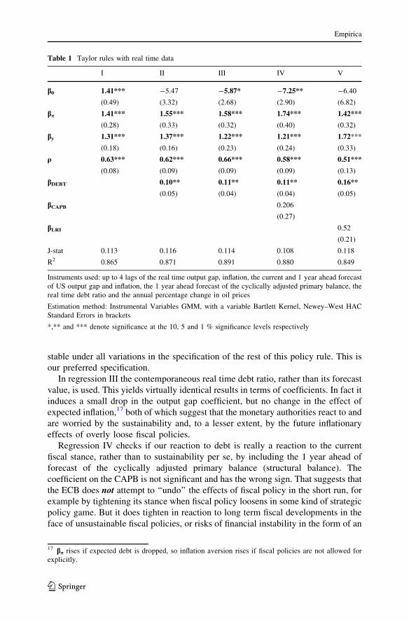
stable under all variations in the specification of the rest of this policy rule. This is

our preferred specification.

In regression III the contemporaneous real time debt ratio, rather than its forecast

value, is used. This yields virtually identical results in terms of coefficients. In fact it

induces a small drop in the output gap coefficient, but no change in the effect of

expected inflation,17 both of which suggest that the monetary authorities react to and

are worried by the sustainability and, to a lesser extent, by the future inflationary

effects of overly loose fiscal policies.

Regression IV checks if our reaction to debt is really a reaction to the current

fiscal stance, rather than to sustainability per se, by including the 1 year ahead of

forecast of the cyclically adjusted primary balance (structural balance). The

coefficient on the CAPB is not significant and has the wrong sign. That suggests that

the ECB does not attempt to ‘‘undo’’ the effects of fiscal policy in the short run, for

example by tightening its stance when fiscal policy loosens in some kind of strategic

policy game. But it does tighten in reaction to long term fiscal developments in the

face of unsustainable fiscal policies, or risks of financial instability in the form of an

Table 1 Taylor rules with real time data

I II III IV V

b0 1.41***

(0.49)

-5.47

(3.32)

-5.87*

(2.68)

-7.25**

(2.90)

-6.40

(6.82)

bp 1.41***

(0.28)

1.55***

(0.33)

1.58***

(0.32)

1.74***

(0.40)

1.42***

(0.32)

by 1.31***

(0.18)

1.37***

(0.16)

1.22***

(0.23)

1.21***

(0.24)

1.72***

(0.33)

q 0.63***

(0.08)

0.62***

(0.09)

0.66***

(0.09)

0.58***

(0.09)

0.51***

(0.13)

bDEBT 0.10**

(0.05)

0.11**

(0.04)

0.11**

(0.04)

0.16**

(0.05)

bCAPB 0.206

(0.27)

bLRI 0.52

(0.21)

J-stat 0.113 0.116 0.114 0.108 0.118

R2 0.865 0.871 0.891 0.880 0.849

Instruments used: up to 4 lags of the real time output gap, inflation, the current and 1 year ahead forecast

of US output gap and inflation, the 1 year ahead forecast of the cyclically adjusted primary balance, the

real time debt ratio and the annual percentage change in oil prices

Estimation method: Instrumental Variables GMM, with a variable Bartlett Kernel, Newey–West HAC

Standard Errors in brackets

*,** and *** denote significance at the 10, 5 and 1 % significance levels respectively

17 bp rises if expected debt is dropped, so inflation aversion rises if fiscal policies are not allowed for

explicitly.

Empirica

123

excessive build-up of debt.18 We have extended this regression to test for the

possibility of an asymmetry or threshold effect in the ECB’s responses to large fiscal

deficits. However, replacing CAPB by its squared value did not produce a

significant coefficient.

Finally Regression V includes long term interest rates (the rate on 10 year

government bonds) among the explanatory variables. Long rates are, in the

traditional view of the yield curve, partly influenced by inflationary pressures to be

expected in the future. However the ECB appears not to respond to such indicators.

Again this suggests that the ECB is more concerned to ensure fiscal sustainability

directly, there being sufficient terms representing future inflation pressures

elsewhere in their policy rule. The implication is they react to debt directly because

there is little advantage in trying to supplement market discipline (influence the

yield curve) through short rates since they cannot rely on long rates being increased

that way.

One concern with these results is that the reaction of interest rates to debt could

be an artefact of reverse causality—i.e. higher policy rates lead to higher rates at the

long end of the yield curve which push up debt service costs and hence the debt ratio

itself. Three pieces of evidence allay this fear. First, when the long run interest rate

Table 2 Taylor rules with ex post data

I II III

b0 0.758***

(0.03)

0.604***

(0.03)

-10.31**

(5.03)

bp 1.14***

(0.12)

0.49***

(0.05)

1.75***

(0.33)

by 0.85***

(0.08)

0.90***

(0.05)

1.08***

(0.103)

q 0.758***

(0.03)

0.604***

(0.03)

0.743***

(0.04)

bDEBT -0.118***

(0.012)

0.147**

(0.07)

J-stat 0.208 0.164 0.159

R2 0.884 0.820 0.808

Instruments used: up to 4 lags each of the ex post output gap, inflation, the ex-post US output gap and

inflation, ex post cyclically adjusted budget, ex-post debt ratio and the annual percentage change in oil

prices

Estimation method: Instrumental Variables GMM, with a variable Bartlett Kernel, Newey–West HAC

Standard Errors in brackets

*,** and *** denote significance at the 10, 5 and 1 % significance levels respectively

18 This result suggests a competitive debt game, not the deficit-interest rate game traditionally described

in the literature. The presence of debt in the ECB’s reaction implies some kind of debt target in which the

ECB aims to clear up past fiscal excesses. See Hughes Hallett (2008b). But without the corresponding

fiscal reaction functions, we cannot tell the form of the implicit policy game (Nash non-cooperative, or

Stackelberg with fiscal or monetary leadership).

Empirica

123

is included in the Taylor rule in its own right, it is not significant. If the reverse

causality story were true, then it would show up in a long-term interest rate term as

well as (or even instead of) the debt ratio. Second, when the 1 year ahead forecast of

debt is instrumented to take account of the simultaneity that would underlie any

possible reverse causality, the coefficient on debt remains significant and of a very

similar size. Indeed the coefficient on debt remains significant even when more

distant lags are used as instruments. Third, our coefficient implies a 25 basis point

rise in the policy rate is associated with a 250 basis point rise in the debt to GDP

ratio under reverse causality. It is implausible that such a small rise in the policy rate

could cause such a large change in the debt ratio.19

3.3 Results with ex-post data

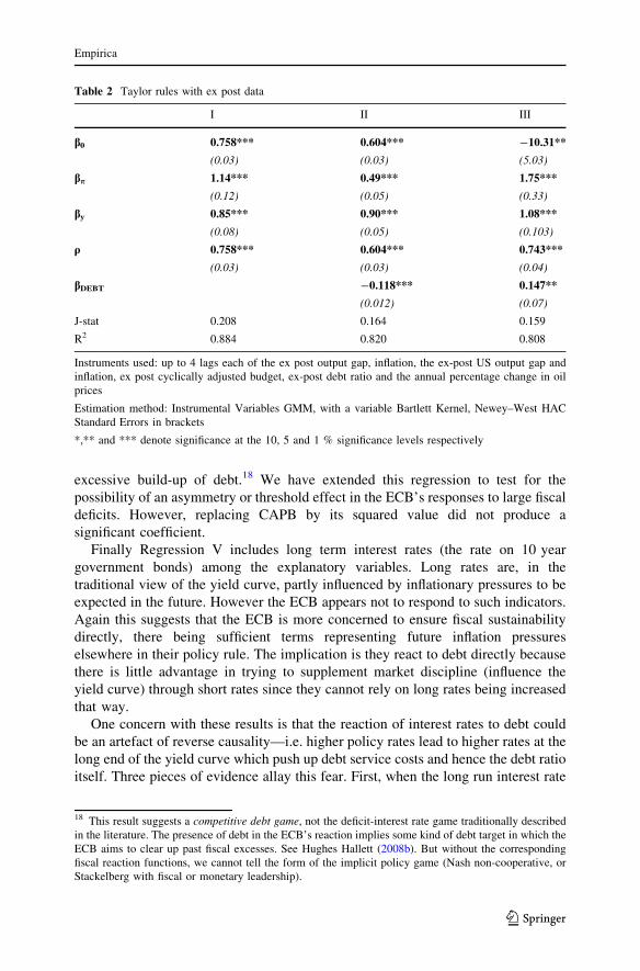
By way of contrast, Table 2 presents the corresponding Taylor rules estimated with

ex-post data.

We use the same variables as instruments, but take the ex-post observations to do

so. In keeping with our rational expectations formulation, we do not include forward

looking ex-post variables as instruments.

These ex-post regressions show that the outcomes of the ECB’s behaviour, as it

turns out, have been rather different from what the ECB originally intended—but

not with respect to loose fiscal policies that lead to high debt. Regression I, the

canonical Taylor rule, implies that the ECB, when it comes to ex-post results,

appears to pay a lot less attention to inflation than originally intended and only just

respects the Taylor principle. It also appears to pay less attention to the output gap.

What has taken the place of those two determinants of monetary policy is a 50 %

increase in policy persistence. Inertia is an important facet of implementation.

This group of results require further explanation. The action in going from real

time to ex-post data is predominantly in the output gap variable. In fact, as nearly

always in studies of this kind, the data actually shows a significant increase in the

variability in the output gap figures (relative to target) in ex-post as compared to real

time figures—mostly because of the revisions to the official estimates of trend or

potential output. So the softening of the ECB’s apparent reactions to inflation and

output is exactly what we should expect as we move from real time to ex post: the

variance of the explanatory variable has increased in ex-post data, while that of the

dependent variable has not.

But when we come on to the reactions to debt and fiscal policy we find a second,

and possibly more interesting set of results. If we take the case of future debt ratios,

as forecasted 1 year ahead (regression II), we find that the ECB lowers interest rates

when there is a projected build-up of debt. This might appear to be the wrong

reaction (wrong sign). But since this is based on ex post data, this does not reflect a

genuine reaction.

19 Suppose there was a one for one pass-through of interest rate changes; a 25 basis point rise in the

policy rate would lead to a 25 basis point rise in the long term rate. If debt was initially 60 % of GDP,

then this would lead to a 15 basis point rise in the debt to GDP ratio. Yet under reverse causality, the

coefficient from our regression would imply a 250 basis point rise in the debt to GDP ratio. That is not a

plausible result for the Euro-zone as a whole.

Empirica

123

By contrast, Regression III shows that the story is quite different when it comes

to the current level of debt. If past policies have led to too high a level of public

sector debt then, for a given level of inflation and output gap, monetary policy will

tighten. In fact all the characteristics from the standard Taylor rule return, but in

stronger form. The Taylor principle with respect to inflation is stronger for the same

degree of concern for the output gap; and policy persistence is again 50 % larger

than in the real time results. The implication of this pair of results (II and III) is that

the ECB compromises when current conditions indicate reflation is needed, but

continues to try to offset the effects of fiscal excesses that have happened in the past.

This explains why the ECB tried to raise interest rates under austerity policies in

2011, but lowered them again 4 months later.

4 Conclusions

Estimating a reaction function for the central bank or fiscal authority using real time

data yields different characterisations of policymaker behaviour compared to when

ex post data is used. In our application, we get a different interpretation of ECB

behaviour if we use ex-post data in place of real time data, and would then miss

being able to uncover what the ECB really intended to do. In fact, using real time

data, we find evidence that the ECB does take fiscal imbalances into account when

setting monetary policy. While they do not respond to the current fiscal stance, as

represented by the cyclically adjusted primary balance, they do respond to debt. A

100 basis point (1 percentage point) rise in the debt to GDP ratio is associated with a

10 basis point rise in interest rates.

Thus, in real time, monetary and fiscal policies do appear to conflict. The form of

the policy game is not yet clear. It could be non-cooperative. But our results suggest

that it is likely to be a leadership game with monetary dominance since the ECB

appears to be reacting to problems of long run fiscal sustainability, rather than trying

to undo large deficits when fiscal policy responds with an expansion. But we need to

uncover the corresponding fiscal reactions to confirm this asymmetry. To do that

properly would be problematic since there are 17 different reaction functions to take

into account. One might operate with an average euro-fiscal reaction function. But,

if the sovereign debt crisis has taught us anything, it is that fiscal imbalances in

smaller economies are quite sufficient to upset the fiscal stance and monetary

reactions for the Euro-zone as a whole. So averaging the fiscal responses or using an

average euro-function is not likely to reveal anything robust. As it is, one can always

estimate one equation out of a simultaneous model if an appropriate IV estimator,

such as our GMM technique, is used. We leave a solution to the fiscal side of the

problem to a separate paper.

Finally, we have pointed out that the form of the implicit policy game, if there is

one, can be determined from the signs of the coefficients on the rival’s instrument in

each reaction function. In this case our results suggest a non-cooperative game with

monetary leadership. Thus the ECB’s monetary policy is active in the sense of

Leeper (1991). In addition it appears to be stabilising; and as such contrasts with

Cochrane’s (2011) claim that Taylor rules lead to instability. The reason for the

Empirica

123

difference is that Cochrane’s analysis asks a policy rule without forward-looking

elements to control a model with forward-looking behaviour, while the standard

stabilisability property under rational expectations requires a forward-looking rule

for such cases.20 The forward-looking element in our estimates is supplied by the

1 year ahead debt forecast. This explains why the debt term is crucial to our results

and to the ECB’s decisions. The need for such a term is clearer in the sovereign debt

crisis, than it was before that crisis.

If we then go on to ex-post data, it starts to appear (unfairly as the policymakers

could not have used ex-post data) as if they were accommodating fiscal policy. This

explains why many studies have concluded that central banks have been weak,

permissive or accommodating in the past. However that can be a misleading

conclusion, as this paper shows in its real time estimates.

Our results in fact reject the hypothesis that monetary policy passively

accommodates looser fiscal policies. If anything, worsening public finances prompt

a tightening in monetary policy via the debt to GDP ratio. Then, in the ex-post data,

we find the ECB supports expansionary fiscal policies if a need to reflate the

economy is foreseen, but also reacts more aggressively to correct past excesses that

have led to high debt ratios. In that sense, the ECB has been acting responsibly—by

which we mean real time decisions respond to fiscal policy to remove expected

excesses and to preserve sustainable finances; and as a good citizen (by which we

mean the outcomes appear to suggest a degree of coordination, coupled with

increasingly active policy measures to clear up past excesses). This is a more subtle

and more nuanced view of the ECB’s policy role than that traditionally understood.

Going forward, the obvious topics for further study are therefore: (a) To develop

matching fiscal reaction functions; (b) To determine the form of game which

underlies the strategic behaviour identified in this paper; and (c) To determine

whether the variability in output gap figures is the result of shocks or fiscal policy.

Acknowledgments Work on the paper has benefited from John Lewis’ visit to the Robert Schuman

Centre for Advanced Studies at the European University Institute under the Pierre Warner Chair

programme and Andrew Hughes Hallett’s visit to De Nederlandsche Bank under the Visiting Scholar

Programme. The authors thank Fritz Breuss, Kerstin Bernoth, Steven Poelhekke, Efrem Castelnuovo,

Jacopo Cimadomo and Massimo Giuliodori for comments on earlier drafts.

Appendix 1: Stationarity and nonstationarity tests

The most widely used test of stationarity is the Kwiatkowski et al. (1992) test.

Conventional alternatives, which test for nonstationary behaviour with stationarity

as the alternative, are the Augmented Dickey Fuller and Phillips-Perron tests.21 We

20 See Acocella et al (2012), chapter 12, for a detailed discussion of stabilisability under forward looking

expectations.21 A modification of the last, the Ng-Perron test, is also possible. But this produces multiple test statistics

and inconclusive results in our case. The results also depend on detrending the data, implying that the

conclusions may be sensitive to the detrending techniques chosen. We did not pursue the Ng-Perron tests

further therefore.

Empirica

123

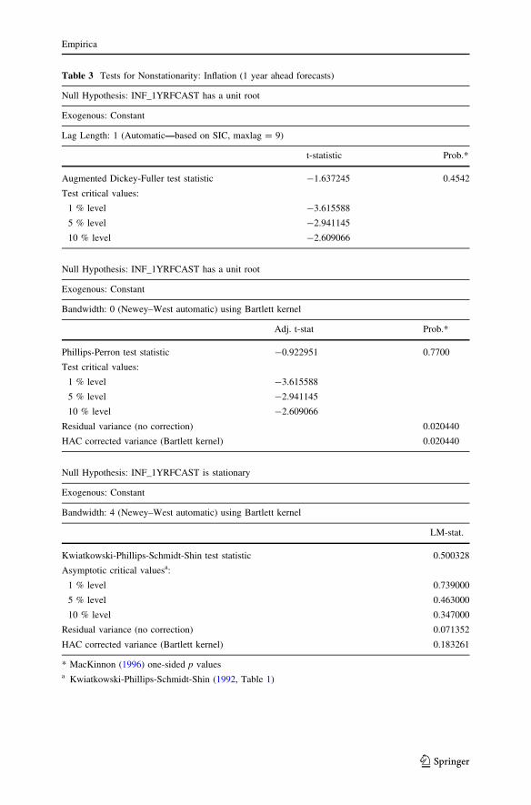
Table 3 Tests for Nonstationarity: Inflation (1 year ahead forecasts)

Null Hypothesis: INF_1YRFCAST has a unit root

Exogenous: Constant

Lag Length: 1 (Automatic—based on SIC, maxlag = 9)

t-statistic Prob.*

Augmented Dickey-Fuller test statistic -1.637245 0.4542

Test critical values:

1 % level -3.615588

5 % level -2.941145

10 % level -2.609066

Null Hypothesis: INF_1YRFCAST has a unit root

Exogenous: Constant

Bandwidth: 0 (Newey–West automatic) using Bartlett kernel

Adj. t-stat Prob.*

Phillips-Perron test statistic -0.922951 0.7700


1 % level -3.615588

5 % level -2.941145

10 % level -2.609066

Residual variance (no correction) 0.020440

HAC corrected variance (Bartlett kernel) 0.020440

Null Hypothesis: INF_1YRFCAST is stationary

Exogenous: Constant


LM-stat.

Kwiatkowski-Phillips-Schmidt-Shin test statistic 0.500328

Asymptotic critical valuesa:

1 % level 0.739000

5 % level 0.463000

10 % level 0.347000



* MacKinnon (1996) one-sided p valuesa Kwiatkowski-Phillips-Schmidt-Shin (1992, Table 1)

Empirica

123

subjected our independent variables to all three tests, with results presented in

Tables 3, 4 and 5 below.

On the face of it, the ADF and PP tests in Tables 3, 4 and 5 might suggest

accepting (at least not rejecting) the null of nonstationarity. However these tests

have always been criticised for being unreliable: that is, of very low power against

Table 4 Tests for Nonstationarity: Output gap (1 year ahead forecasts)

Null Hypothesis: GAP_1YRFCAST has a unit root

Exogenous: Constant


t-statistic Prob.*



1 % level -3.615588

5 % level -2.941145

10 % level -2.609066

Null Hypothesis: GAP_1YRFCAST has a unit root

Exogenous: Constant


Adj. t-stat Prob.*



1 % level -3.615588

5 % level -2.941145

10 % level -2.609066



Null Hypothesis: GAP_1YRFCAST is stationary

Exogenous: Constant


LM-stat.


Asymptotic critical values*

1 % level 0.739000

5 % level 0.463000

10 % level 0.347000

* MacKinnon (1996) one-sided p values

Empirica

123

Table 5 Tests for nonstationarity: Debt to GDP ratio (1 year ahead forecasts)

Null Hypothesis: DEBT_1YRFCAST has a unit root

Exogenous: Constant


t-statistic Prob.*



1 % level -3.621023

5 % level -2.943427

10 % level -2.610263

Null Hypothesis: DEBT_1YRFCAST has a unit root

Exogenous: Constant


Adj. t-stat Prob.*



1 % level -3.621023

5 % level -2.943427

10 % level -2.610263



Null Hypothesis: DEBT_1YRFCAST is stationary

Exogenous: Constant


LM-stat.


Asymptotic critical valuesa:

1 % level 0.739000

5 % level 0.463000

10 % level 0.347000



* MacKinnon (1996) one-sided p valuesa Kwiatkowski-Phillips-Schmidt-Shin (1992, Table 1)

Empirica

123

near nonstationary alternatives22 and as poor asymptotic approximations to the true

test when the number of degrees of freedom is small. And that is the case here. We

only need roots in the data generating process to be just less than one for the

regressions in Tables 1 and 2 to be valid. This makes the test distributions under the

null and alternative hypotheses almost the same. As a result, Tables 3, 4 and 5

shows that the probability of making an inference error if you accept the null

(nonstationarity) is actually higher than the probability of an error if you accept the

alternative (stationarity)—by factors of 1.04–1.4 (except the ADF and PP tests for

inflation). So we can drop these tests as showing more than reasonable doubt about

nonstationarity.

So that leaves us with the KPSS tests, whose type I and type II error probabilities

are in the right proportions to go with stationarity. The probability of an error if we

accept stationarity for debt and the output gap being smaller, by factors of 5 or 6,

than if we accept nonstationarity. Only the 1 year ahead inflation forecasts showed

any tendency to nonstationary behaviour, but even that is marginal at conventional

5 % significance levels. We conclude we have no clear evidence to reject

stationarity.

There are also first principles arguments that support stationarity. (1) If a variable

is bounded above and below in practice (like unemployment) it cannot be

nonstationary, although it might still show ‘‘local’’ nonstationary behaviour in

particular samples of data. Both the output gap and the debt-to-GDP ratio are cases

in point: the former because, by definition, it has a long run value of zero; the latter

because it cannot be negative or exceed a sustainable level without a collapse,

default or an austerity programme imposed: see Ghosh et al. (2011). (2) Given that

all three variables are weighted averages over the Eurozone up to 2008, there is

nothing in the data to suggest nonstationarity (whether forecast, current or expost

values): see Fig. 1. In fact, debt and the output gap were declining as euro averages

over that period; debt from 72 % in 1999 to 66 % of GDP in 2008, the output gap

from -0.2 % to 1 % of GDP. Inflation is less clear, as the stationarity tests imply. It

was 1.7 % in 1999, 2.4 % in 2001, 2.1 % in 2007 and 3.7 % in 2008.

Appendix 2: Alternative specifications for Table 1

The tables below display alternative estimates for Table 1 to underline the

robustness of our preferred regression. For convenience, panel A reproduces

Regression II to aid comparison with the two following cases: OLS estimates of the

same regression, and the same omitting the debt ratio variable. The argument for

introducing OLS estimates is that GMM estimates are some-times sensitive to small

variations in specification or the set of instrument variables employed. And so it is

here, except that it is the OLS estimates that are sensitive to ignoring simultaneity

biases. The OLS estimates themselves are uniformly insignificant which makes no

sense since it implies that monetary policy is simply a predetermined AR process

with zero interest rates on average (the constant is insignificant). In other words, the

22 Dufour and King (1991).

Empirica

123

Table 6 Alternative estimates of the ECB’s policy reaction function

Panel (A): Regression II, Dependent Variable: IE

Method: Generalized Method of Moments

Included observations: 37 after adjustments

Kernel: Bartlett, Bandwidth: Variable Newey–West (4), No prewhitening

Convergence achieved after: 103 weight matrices, 104 coefficient iterations

IE = C(1)*IE(-1) ? (1-C(1))*(C(2) ? C(3)*INF_1YRFCAST ? C(4)

*GAP_1YRFCAST ? C(5)*DEBT_1YRFCAST)

Instrument specification: IE(-1) C GAP_RT(-1 TO -4) INF_OWN(-1 TO -4)

USGAP_RT USINF_RT USGAP_1YRFCAST USINF_1YRFCAST

CAPB_1YRFCAST DEBT_RT OIL

Coefficient Std. Error t-statistic Prob.

C(1) 0.616318 0.082951 7.429923 0.0000

C(2) -5.478022 3.324053 -1.647995 0.1091

C(3) 1.554901 0.331299 4.693343 0.0000

C(4) 1.379767 0.158065 8.729133 0.0000

C(5) 0.103819 0.046745 2.220960 0.0336

R-squared 0.870599 Mean dependent var 3.262432

Panel (B): Regression II, Dependent Variable: IE

Method: Least Squares

Included observations: 37 after adjustments

Convergence achieved after 16 iterations

IE = C(1)*IE(-1) ? (1-C(1))*(C(2) ? C(3)*INF_1YRFCAST ? C(4)

*GAP_1YRFCAST ? C(5)*DEBT_1YRFCAST)


C(1) 0.924610 0.125585 7.362436 0.0000

C(2) -60.93883 120.3130 -0.506502 0.6160

C(3) 5.853011 9.098876 0.643267 0.5246

C(4) 2.851259 4.122870 0.691571 0.4942

C(5) 0.891433 1.733183 0.514333 0.6106

R-squared 0.909754

Adjusted R-squared 0.898473

S.E. of regression 0.311241

Sum squared resid 3.099878

Log likelihood -6.628955

Durbin-Watson stat 1.232496

Mean dependent var 3.262432

S.D. dependent var 0.976804

Akaike info criterion 0.628592

Schwarz criterion 0.846284

Hannan-Quinn criter. 0.705339

Empirica

123

ECB is totally passive and takes no decisions. Since we know that not to be true, we

can dismiss this variation (Table 6).

Panel C, dropping the debt variable, produces an inferior outcome for both

inflation and the output gap without a measurable improvement in fit or other

diagnostics. The implication is that real or structural indicators of economic

performance are important to ECB monetary policy.

References

Acocella N, Di Bartolomeo G, Hughes Hallett A (2012) The theory of economic policy in a strategic

context. Cambridge University Press, Cambridge and New York

Alesina A, Blanchard O, Galı J, Giavazzi F, Uhlig H (2001) Defining a macroeconomic framework for the

Euro area, monitoring the European Central Bank 3. Centre for Economic Policy Research, London

Beetsma R, Uhlig H (2000) An analysis of the stability and growth pact. Economic Journal 109:546–571

Begg D, De Grauwe P, Giavazzi F, Uhlig H, Wyplosz C (1998) The ECB: safe at any speed? Monitoring

the European Central Bank. Centre for Economic Policy Research, London

Belke A, Klose J (2011) Does the ECB rely on a Taylor rule during the financial crisis? Comparing ex-

post and real time data with real time forecasts. Econ Anal Policy 41:147–171

Bernanke B, Gertler M (2001) Should Central banks respond to movements in asset prices? Am Econ Rev

91:253–257

Table 6 continued

Panel (C): No debt, Dependent Variable: IE

Method: Least Squares

Included observations: 38

Convergence achieved after 21 iterations

IE = C(1)*IE(-1) ? (1 - C(1))*(C(2) ? C(3)*INF_1YRFCAST ? C(4)

*GAP_1YRFCAST)


C(1) 0.815523 0.114830 7.102023 0.0000

C(2) -0.459695 2.271633 -0.202363 0.8408

C(3) 2.204948 1.205258 1.829441 0.0761

C(4) 0.772179 0.298156 2.589846 0.0140

R-squared 0.903780

Adjusted R-squared 0.895290

S.E. of regression 0.323980

Sum squared resid 3.568748

Log likelihood -8.977609

Durbin-Watson stat 0.833838

Mean dependent var 3.306579

S.D. dependent var 1.001208

Akaike info criterion 0.683032

Schwarz criterion 0.855410

Hannan-Quinn criter. 0.744363

Empirica

123

Bini Smaghi L (2007) Central bank independence: from theory to practice, speech given to Hungarian

National Assembly, http://www.ecb.int/press/key/date/2007/html/sp070419.en.html

Bordo M, Jeanne O (2002) Monetary policy and asset prices: does benign neglect make sense? Int Financ

5:139–164

Carstensen K, Colavecchio R (2004) Did the revision of the ECB monetary policy strategy affect the

reaction function? Kiel Working Paper No. 1221

Castelnuovo E (2007) Taylor rules and interest rate smoothing in the euro area. Manch School 75:1–16

Cecchetti S, Genberg H, Wadhwani S (2002) Asset prices in a flexible inflation targeting framework. In:

Hunter WC, Kaufman GG, Pomerleano M (eds) Asset price bubbles: implications for monetary,

regulatory and international policies. MIT Press, Cambridge, MA

Chari V, Kehoe P (2003) On the need for fiscal constraints in a monetary union. J Monet Econ

54:2399–2408

Cimadomo J (2011) Real time data and fiscal policy analysis: a survey of the literature. WP 11-25 Federal

Reserve Bank of Philadelphia, Philadelphia

Cochrane J (2009) ‘‘Fiscal Theory, and Fiscal and Monetary Policy in the Financial Crisis’’ paper

presented to the conference ‘‘Monetary-Fiscal Interactions, Expectations and Dynamics in the

Current Economic Crisis’’, Princeton University, Princeton NJ (22–23 May, 2009)

Cochrane J (2011) Determinancy and identification with Taylor rules. J Polit Econ 119:565–615

Coenen G, Levin A, Wieland V (2003) Data uncertainty and the role of money as an information variable

for monetary policy. Eur Econ Rev 49:975–1006

Dixit A, Lambertini L (2003) Symbiosis of monetary and fiscal policies in a monetary union. J Int Econ

60:235–247

Dufour J-M, King M (1991) Optimal Invariant tests for the autocorrelation coefficient in linear

regressions with stationary and nonstationary AR(1) errors. J Econom 47:115–143

Duisenburg W (2001) Current fiscal and monetary policy issues in the Euro area, speech given to the

Taxpayers Association of Europe, 12 December http://www.ecb.int/press/key/date/2001/html/

sp011207.en.html

Euspei S, Preston B (2010) Central bank communications and expectations stabilisation. Am Econ J

Macro 2:235–271

Fourcans A, Vranceanu R (2004) The ECB interest rate under the duisenburg presidency. Eur J Polit Econ

20:579–595

Gerdesmeier D, Roffia B (2004) Taylor rules for the euro area: the issue of real time data. Deutsche

Bundesbank, Discussion Paper No 37/2004

Gerlach S (2007) Interest rate setting by the ECB, 1999–2006: words and deeds. Int J Central Bank

3:1–45

Gerlach S, Lewis J (2010) The zero lower bound, ECB interest rate policy and the financial crisis. DNB

Working Paper 254, Netherlands Central Bank, Amsterdam

Gerlach-Kristen P (2003) Interest rate reaction functions and the Taylor rule in the Euro area. ECB

Working Paper 258, European Central Bank, Frankfurt

Ghosh AR, Kim J, Mendoza E, Ostry JD, Qureshi M (2011) Fiscal Fatigue, Fiscal Space and Debt

Sustainability in Advanced Economies, NBER WP 16782. National Bureau of Economic Research,

Cambridge

Goodfriend M (2009) Central banking in the credit turmoil: an assessment of Federal Reserve practice In:

Paper presented to the conference ‘‘monetary-fiscal interactions, expectations and dynamics in the

current economic crisis’’. Princeton University, Princeton NJ (22–23 May, 2009)

Gorter J, Jacobs J, De Haan J (2008) Taylor rules for the ECB using expectations data. Scand J Econ

110(3):473–488

Hughes Hallett A (1986) Autonomy and the choice of policy in asymmetrically dependent economies.

Oxf Econ Pap 38:516–544

Hughes Hallett A (2008a) Post-Thatcher fiscal policies in the United Kingdom. In: Neck R, Sturm J-E

(eds) Sustainability of Public Debt. MIT Press, Cambridge MA

Hughes Hallett A (2008b) Debt targets and fiscal sustainability in an era of monetary independence. IEEP

5:165–187

Hughes Hallett A, Libich J, Stehlik P (2011) Macro-prudential Policies and Financial Stability. Econ

Record 87:318–334

Hughes Hallett A, Kattai R, Lewis J (2012) How reliable are cyclically adjusted budget balances in real

time? Contemp Econ Policy 30:75–92

Empirica

123

http://www.ecb.int/press/key/date/2007/html/sp070419.en.html



Issing O (2004) ‘‘A framework for Stability in Europe’’, speech given at the University of London, 19

November: http://www.bis.org/review/r041130h.pdf

Kwiatkowski D, Phillips P, Schmidt P, Shin Y-C (1992) Testing the null hypothesis of stationarity against

the alternative of a unit root: how sure are we that economic time-series have a unit root? J Monet

Econ 54:159–178

Leeper E (1991) Equilibria under active and passive monetary and fiscal policies. J Monet Econ

27:129–147

Leeper E (2009) Anchoring fiscal expectations, Reserve Bank of New Zealand Bulletin 72:7–32; and

NBER working paper 15629, NBER, Cambridge, MA

Lisman J, Sandee J (1967) Interpolation of quarterly figures from annual data. Appl Stat 13:87–90

MacKinnon JG (1996) Numerical distribution functions for unit root and cointegration tests. J Appl

Econom 11:601–618

Melitz J (2002) Debt, Deficits and the behaviour of monetary and fiscal policies. In: Buti M, Martinez-

Mongay C, von Hagen J (eds) The behaviour of fiscal authorities: stabilisation, growth and

institutions. Palgrave-MacMillan, Basingstoke

Mishkin F (2002) The role of output stabilisation in the conduct of monetary policy. Int Financ 5:2–13

Newey W, West K (1994) Automatic lag selection in covariance matrix estimation. Rev Econ Stud

61:631–654

Orphanides A (2001) Monetary policy rules based on real-time data. Am Econ Rev 91:964–985

Sauer J, Sturm J (2007) Using Taylor rules to understand european central bank monetary policy. German

Econ Rev 8:375–398

Staiger DO, Stock J (1997) Instrumental variables regression with weak instruments. Econometrica

65:557–586

Stock J, Yogo M (2005) Testing for Weak Instruments in Linear IV Regression. In: Andrews D, Stock J

(eds) Identification and inference for econometric models: essays in honor of thomas rothenberg.

Cambridge University Press, Cambridge and New York

Surico P (2003) Asymmetric reaction functions for the euro area. Oxf Rev Econ Policy 19(1):44–57

Svensson L (1997) Inflation forecast targeting: implementing and monitoring inflation targets. Eur Econ

Rev 41:1111–1146

Svensson L (2003) What is wrong with Taylor rules? Using judgment in monetary policy through

targeting. J Econ Lit 41:426–477

Wyploz C (1999) Towards a More Perfect EMU, Discussion Paper 2252. Centre for Economic Policy

Research, London

Empirica

123

http://www.bis.org/review/r041130h.pdf

monetary policy and sovereign debt: does the ecb take the eurozone’s fiscal risks into account?

Documents