mohammad hossein manshaei manshaei@gmail

Mohammad Hossein Manshaei [email protected]

Chapter 11: (secowinet.epfl.ch) Multi-domain sensor networks, Border games in cellular networks

2

11.1 Multi-domain sensor networks 11.2 Border games in cellular networks

3

Ø Typical cooperation: help in packet forwarding Ø Can cooperation emerge spontaneously in

multi-domain sensor networks based solely on the self-interest of the sensor operators?

4

•  C: Cooperation D: Defection

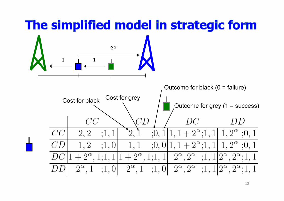
•  4 possible moves: •  CC – the sensor asks for help (cost 1) and helps if asked (cost 1) •  CD – the sensor asks for help (cost 1) and does not help (cost 0) •  DC – the sensor sends directly (cost 2α) and helps if asked (cost 1) •  DD – the sensor sends directly (cost 2α) and does not help (cost 0)

2α

1 1

1 1 1

5

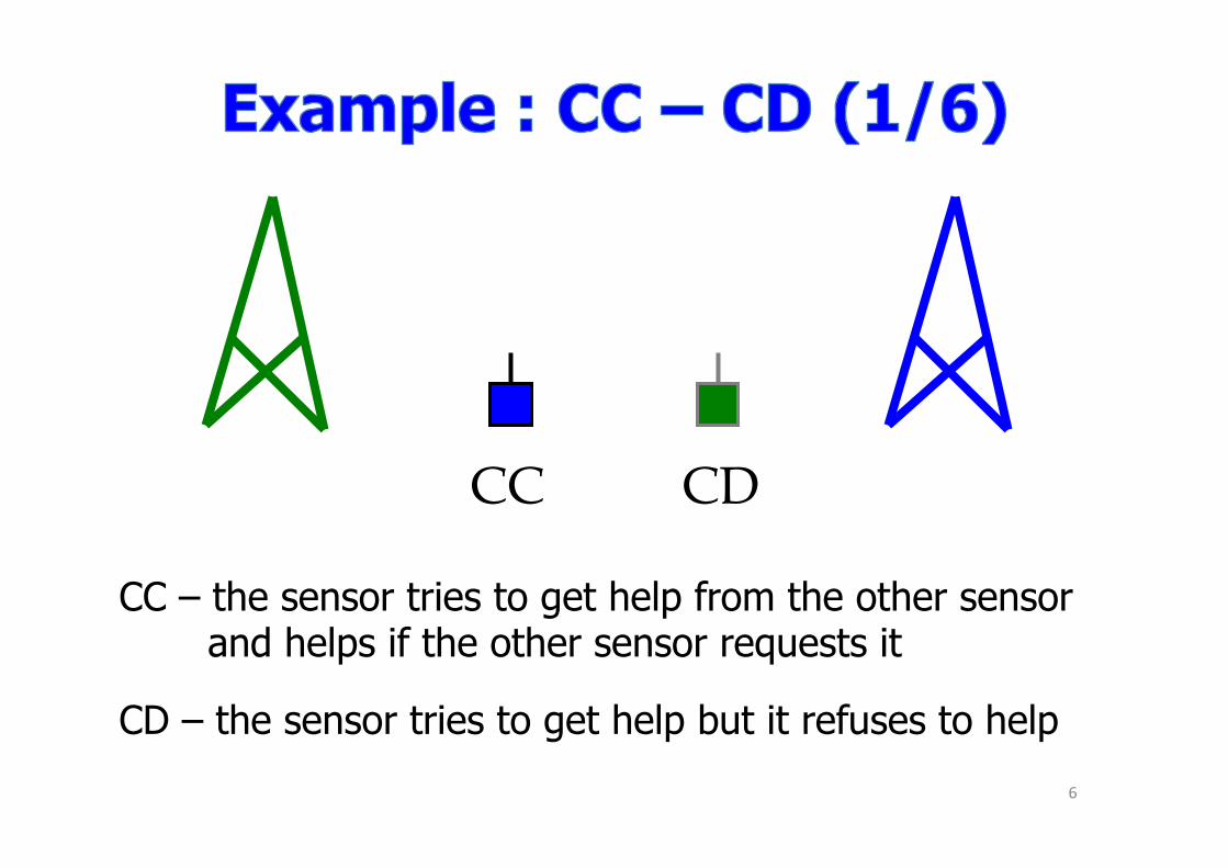
CC – the sensor tries to get help from the other sensor and helps if the other sensor requests it

CD – the sensor tries to get help but it refuses to help

CC CD

6



CC CD

7

CC failure

CD



8

CC CD



9

CC CD success

10

CC CD

Black player

Cost: 2

•  1 for asking

•  1 for helping

Benefit: 0

(packet dropped)

Gray player

Cost: 1

•  1 for asking

Benefit: 1

(packet arrived)

11

2α

1 1

Cost for black Cost for grey

Outcome for black (0 = failure)

Outcome for grey (1 = success)

12

time

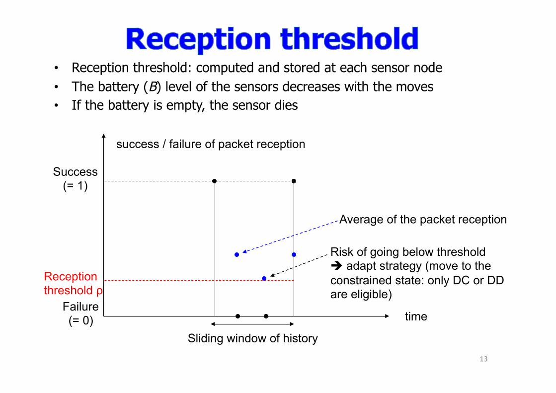
success / failure of packet reception

Sliding window of history

Success (= 1)

Failure (= 0)

Reception threshold ρ

Average of the packet reception

Risk of going below threshold è adapt strategy (move to the constrained state: only DC or DD are eligible)

•  Reception threshold: computed and stored at each sensor node •  The battery (B) level of the sensors decreases with the moves •  If the battery is empty, the sensor dies

13

•  The mentioned concepts describe a game •  Players: network operators •  Moves (unconstrained state): CC, CD, DC, DD •  Moves (constrained state): DC, DD •  Information sets: histories •  Strategy: function that assigns a move to every

possible history considering the weight threshold •  Payoff = lifetime •  We are searching for Nash equilibria with the

highest lifetimes

14

B – initial battery

ρ – reception threshold

α – path loss exponent (≥2)

ε1,2 – payoff of transient states

Cooperative Nash equilibrium

Non-cooperative Nash equilibrium

If ρ > 1/3, then (CC/DD, CC/DD) is more desirable

15/33

Simplified model with the following extensions: –  many sensors, random placing –  minimum energy path routing –  common sink / separate sink scenarios –  classification of equilibria

•  Class 0: no cooperation (no packet is relayed) •  Class 1: semi cooperation (some packets are relayed) •  Class 2: full cooperation (all packets are relayed)

16

Parameter Value

Number of sensors per domain 20

Area size 100 x 100 m

Reception threshold ρ 0.6

History length 5

Path loss exponent 2–3–4 (3)

17/33

Perc

enta

ge o

f si

mul

atio

ns

Equilibrium classes ( 0 – no cooperation, 1 – semi cooperation, 2 – full cooperation)

Value of the path loss exponent

– 2

– 3

– 4

18

•  We examined whether cooperation is possible without the usage of incentives in multi-domain sensor networks

•  In the simplified model, the best Nash equilibria consist of cooperative strategies

•  In the generalized model, the best Nash equilibria belong to the cooperative classes in most of the cases

19

11.1 Multi-domain sensor networks 11.2 Border games in cellular networks

20

•  spectrum licenses do not regulate access over national borders

•  adjust pilot power to attract more users

Is there an incentive for operators to apply competitive pilot power control?

22

Network: •  cellular networks using CDMA

–  channels defined by orthogonal codes

•  two operators: A and B •  one base station each •  pilot signal power control

Users: •  roaming users •  users uniformly distributed •  select the best quality BS •  selection based signal-to-

interference-plus-noise ratio (SINR)

23

0

pilotp i ivpilot

iv pilot pilotown other

G P gSINR

N I I⋅ ⋅

=⋅ + +W

i

pilotown iv iw

wI g Tς

∈

⎛ ⎞= ⋅ ⋅⎜ ⎟⎜ ⎟

⎝ ⎠∑M

i

pilotother jv j iw

j i wI g P Tη

≠ ∈

⎛ ⎞= ⋅ ⋅ +⎜ ⎟⎜ ⎟

⎝ ⎠∑ ∑

M

A B v

PA PB

TAv

TBw TAw

0

trp iv ivtr

iv tr trown other

G T gSINR

N I I⋅ ⋅

=⋅ + +W

, i

pilotown iv i iw

w v wI g P Tς

≠ ∈

⎛ ⎞= ⋅ ⋅ +⎜ ⎟⎜ ⎟

⎝ ⎠∑

Mtr pilotother otherI I=

pilot signal SINR:

traffic signal SINR:

Pi – pilot power of i

– processing gain for the pilot signal pilotpG

ivg

0N – noise energy per symbol

W

ς

ivT

η

pilotownI

– channel gain between BS i and user v

– available bandwidth

– own-cell interference affecting the pilot signal

– own-cell interference factor

– traffic power between BS i and user v

– other-to-own-cell interference factor

iM – set of users attached to BS i

24

•  Power Control Game, GPC

– players → networks operators (BSs), A and B – strategy → pilot signal power, 0W < Pi < 10W,

i = {A, B} – standard power, PS = 2W – payoff → profit, where is the

expected income serving user v – normalized payoff difference:

i

i vv

u θ∈

= ∑M vθ

( ) ( )( )( )

max , ,

,i

S S Si i is

i S Si

u s P u P P

u P P

−Δ =

25

•  only A is strategic (B uses PB = PS) •  10 data users •  path loss exponent, α = 2

Δi

27

•  10 data users •  path loss exponent, α = 4

28

10 data users 100 data users

29

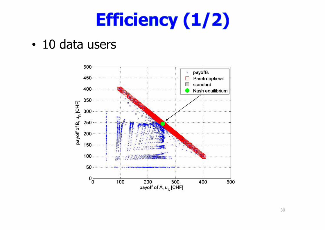
•  10 data users

30

•  100 data users

31

•  convergence based on better-response dynamics •  convergence step: 2 W

PA = 6.5 W

32

•  convergence step: 0.1 W

33

•  not only individual nodes may exhibit selfish behavior, but operators can be selfish too

•  example: adjusting pilot power to attract more users at national borders

•  the problem can be modeled as a game between the operators –  the game has an efficient Nash equilibrium –  there’s a simple convergence algorithm that

drives the system into the Nash equilibrium

34

mohammad hossein manshaei manshaei@gmail

Documents