modified bar gauges - core.ac.uk between the front disk and the sensing ... film was glued around...
TRANSCRIPT

Modified Bar Gauges
H. H. Sam Chiu and David J. Mee
Centre for HypersonicsDivision of Mechanical Engineering
The University of Queensland. Australia.
The University of QueenslandDivision of Mechanical EngineeringResearch Report Number 2003/22

Abstract
This report presents the results of a study into the development of bar gauges for the
measurement of Pitot pressures in low density expansion tube flows. The bar gauges
developed here are modified from the conventional designs for bar gauges. A steel
disc of 9 mm diameter and 1 mm thickness is attached to the front of a shielded
sensing bar. Semiconductor strain gauges are used as the strain sensing elements. A
PCB impact hammer was used to calibrate the bar gauges. Experiments in flows at 9
km/s, with Pitot pressures close to 750 kPa, were done in the X1 expansion tube at
The University of Queensland. Tests were also performed by changing the operation
mode of the X1 facility to run it as a non-reflected shock tunnel. For those tests the
flow speed was around 1.3 km/s and the Pitot pressure was close to 650 kPa. This test
flow was used to check the calibration of the bar gauges. The results indicate that the
bar gauges developed here can be used to measure Pitot pressures in flows with a test
period of up to 100 µs. The quality of the signals can be enhanced by ensuring good
contact between the front disk and the sensing bar. Moreover, by isolating the sensing
bar electrically from the tunnel the effects of ionisation on noise levels on the strain
signal is reduced. In order to obtain the true Pitot pressure measurements, the average
disc pressures measured using the presented bar gauges have to be multiplied by a
factor of 1.08 (1/0.93). The overall uncertainty of the Pitot pressure measured is
estimated to be ± 7%, for Pitot pressures of order 600 kPa.

TABLE OF CONTENTS
Abstract
Table of contents
List of Tables and Figures
1. Introduction / History 1
2. New Bar Gauge 4
2.1 Principle of operation of the new bar gauge 4
2.2 Strain sensing elements 5
2.3 Calibration 6
2.3.1 Hammer test 6
2.3.2 Shock tube test 6
3. Comparison between four different pressure measurement devices 9
4. Noise on bar gauge signals 14
4.1 Identification of the sources of the spikes on strain sensors 16
4.2 Minimising the effects of noise on the strain gauge signals 20
4.2.1 Position of strain gauges 20
4.2.2 Use of semiconductor strain gauges 21
4.2.3 Electrically isolation of the sensing bar 22
4.2.4 Contact between the disc and the sensing bar 23
4.3 Summary 25
5. Uncertainties for bar gauges 26
5.1 Sensitivity to the dimensions of the disc 26
5.2 Uncertainties between average disc pressure and true Pitot pressure 26
5.3 Uncertainty in strain signal variation 27
5.4 Uncertainty in the Pitot pressure measurements using the bar gauges 27

6. Conclusion 28
7. Reference 29
Appendix A Manufacture and Instrumentation of the Bar Gauges 31
A.1. Electrical circuit 32
A.2. Semi-conductor Strain Gauge information 33
A.3. Installation for gauges 34
Appendix B Experimental data by shots 39

LIST OF TABLES AND FIGURES
Tables
Table 1 Nominal shock tube flow conditions at the exit of the tube 8
Table 2 Locations of strain sensors on each probe 12
Figures
Figure 1 Shield PCB piezoelectric pressure transducer Pitot probe 1
Figure 2 Original stress wave bar 2
Figure 3 Sutcli ffe’s re-designed stress wave bar gauge 2
Figure 4 Present modified stress wave bar gauge 4
Figure 5 Schematic of the X1 expansion tube 7
Figure 6 Modified shock tube arrangement 7
Figure 7 Pressure measurements 9
Figure 8 Comparison between different Pitot probes with flow
arriving times correction 11
Figure 9 Comparison between different types of Pitot probes
with signals normalised by the static pressure at location at8
and with time correction 12
Figure 10 Ideal time history trace when a constant force acts on a bar 14
Figure 11 Sample traces of measured pressure from bar gauges 15
Figure 12 Typical signals from the shock tunnel test 17
Figure 13 Pressure measurement results from bar gauges (from s8_39) 19
Figure 14 Pressure measurement results from bar gauges (from s10_16) 22
Figure 15 Improvement on bar gauges 24

1
1. Introduction/History
Typical test times in expansion tubes are in the order of 50 µs. Because of these short
test times, it has been difficult to measure the Pitot pressures. A suitable instrument
for measuring Pitot pressures should be able to respond quickly and have a high signal
to noise ratio. The most frequently applied methods for measuring Pitot pressures in
these test flows use shielded pressure transducers or stress wave bar gauges.
Pitot pressures are conventionally measured in hypersonic impulse facilities using a
shielded pressure transducer Pitot probe. A standard PCB piezoelectric pressure
transducer shielded inside a pitot probe was used by Neely [1] and Wendt et al. [2] to
measure the Pitot pressure levels in the short duration test flows in the X1 expansion
tube at The University of Queensland.
Figure 1. Shield PCB piezoelectric pressure transducer Pitot probe, taken from [1].
The shielding arrangement was applied to protect the PCB pressure transducer from
damage that might be caused by fragments of the ruptured metallic primary
diaphragm that are convected in the high velocity flow. The cavity between the
transducer and the cover cap in this configuration (see Fig. 1) leads to response times
of the probe of the order of 10 µs. Recent research shows that the time taken to fill
the cavity increases as the level of the density of the flow decreases (refer to [1] and
[4]). This has significant implication for experiments in which rarefied flows are
generated in expansion tubes.
In the late 1970s, bar gauge measurements were first introduced by Mudford et al. [3].
The bar gauges were used for radial pitot surveys of a nozzle in the T3 free-piston
driven shock tunnel. The sensors consisted of a piezo-ceramic element sandwiched

2
between a duralumin bar and a backing bar of lead. They were enclosed in a co-axial
cylindrical shield. The stress signals were transmitted through small wires connecting
the piezo-ceramic element to a mini-plug at the closed end of the bar (refer to Fig. 2).
The response time of these bar gauges was estimated to be less than 2 µs.
Figure 2. Original stress wave bar, taken from [1].
Sutcli ffe [5] redesigned the bar gauges of Neely et al [1] in 1993. The new design (see
Fig. 3) was an improvement on previous designs [3] in terms of reduced response
times and noise levels. The front end of the bar was covered by a piece of brass shim
to protect the instrumentation inside the shielding. A strip of piezoelectric polymer
film was glued around the circumference of the sensing bar. A conductive epoxy was
also used to ensure electrical contact between the sensing bar and the bottom surface
of the film. This forms one output to the transient data recorder with the other being
formed by the top surface of the film. The charge generated when a stress load is
applied to the film is then ampli fied and recorded. Chiu et al [4] reported that this
arrangement can produce large levels of noise if the inner sensing bar comes into
contact with the outer shielding. This can be hard to identify before a test because of
the presence of the front shielding. Also, this type of bar gauge has to be calibrated
individually and is used once only. It would be a time consuming process using this
type of bar gauges to complete a comprehensive Pitot pressure survey of the
flowfield.
Figure 3. Sutcli ffe’s re-designed stress wave bar gauge (not to scale), taken from [5].

3
Therefore, a more reliable and less time consuming process for manufacturing bar
gauges is required so that Pitot pressures surveys can be made in the low-density short
duration test flows in expansion tubes. In order to meet this goal, a newly designed
bar gauge becomes essential. This report presents the results of a study into the
development of bar gauges for the measurement of Pitot pressures in low density
expansion tube flows.
In section 2, the strain sensors and the associated instrumentation of the bar gauges is
described. Then the principle of operating the new bar gauges is given. In addition,
the methods used to calibrate the bar gauges are presented. The calibration results and
the uncertainties are also discussed.
A comparison of results from different Pitot pressure measurement devices is given in
section 3. The performances of these devices are addressed.
Section 4 contains a discussion of noise induced in the strain signals when using the
bar gauges to measure Pitot pressures. This section starts by identifying noise spikes
that occurred regularly on signals from the bar gauges. Then the influence of these
spikes on the results from the gauges is addressed. Lastly, some techniques are
described to minimise the effects of spikes due to the noise.
The uncertainties for bar gauges are discussed and presented in section 5.
In section 6, the conclusions drawn from the study of the new developed bar gauges
are given.
Appendix A presents the manufacture and instrumentation of the bar gauges.

4
2. New Bar Gauge
The bar gauges designed for the present study (Fig. 4) are slightly modified from the
arrangements shown in Figs. 2 and 3. A steel disc of 9 mm diameter and 1 mm
thickness is attached to the front of the bar. This is done to improve the aerodynamic
shielding of the bar and to improve the survivabilit y of the gauge. Although the
addition of a disc will slow the response of the bar gauge, with the present
arrangement the 10% - 90% rise time of the gauge is still only 5 µs. This has been
confirmed by Robinson [9] using Finite Element simulations using NASTRAN (refer
to Fig. 8 in [4]).
Figure 4. Present modified stress wave bar gauge (not to scale).
Two different types of strain sensors were used in the bar gauge – a piezoelectric film
gauge [7] and a semiconductor strain gauge (refer to section 2.2 for details).
Note that the pressure measured using the present bar gauge is the average pressure
acting on the disc. A pressure close to the Pitot pressure would be expected near the
centre of the disc and lower pressures toward the edges of the disc. Therefore, the
average pressure is expected to be lower than the actual Pitot pressure. Bourque [10]
used Direct Simulation Monte Carlo (DSMC) methods and Mee et al. [15] used a
Navier-Stokes code to study the relationship between the average pressure on the disc
and the Pitot pressure. The results show that the average pressure measured using the
present bar gauge will be about 93% of the true Pitot pressure. Therefore, the pressure
indicated by the bar gauge should be multiplied by a factor of 1.08 to determine the
actual Pitot pressure.
2.1 Principle of operation of the new bar gauge
When the flow arrives at the front of the bar, the aerodynamic force on the front disc
generates stress waves that propagate down the bar. These waves travel at the sound

5
speed in the material of which the bar is made. Since the bar is uniform in diameter
and the length to diameter ratio is large the stress wave propagation is approximately
planar and the strain measured at the gauge location can be used to infer the average
pressure acting on the disc attached to the bar. Because it takes a finite time for the
stress waves to propagate from the front of the bar to the location of the gauge, the
output from the gauge indicates the average pressure acting on the front of the bar
with a time delay. This time delay can be calculated using the sound speed in the bar
material and the distance of the strain gauge from the front of the bar. The bar is made
long enough such that the stress waves reflected from the downstream end of the bar
do not reach the gauge until after the end of the test time. For the present arrangement,
brass bars of 4.5 mm diameter and 230 mm length were used and strain gauges were
located approximately 40 mm from the front end of the bar. For this arrangement, the
time available for measurements is approximately 100 µs.
2.2 Strain sensing elements
Piezoelectric film and semiconductor strain gauges were used as the strain sensors to
measure the stress waves propagating down the sensing bars. The strain gauges sense
the strain changes due to the stress waves propagating along the sensing bar. The
strain changes can be converted into voltage changes through charge ampli fiers for
the piezoelectric film gauges and strain gauge ampli fiers for the semiconductor
gauges.
The piezoelectric film, of 10 mm length in the axial direction, was wrapped around
the brass bar with the most sensitive axis of the film being aligned with the axis of the
bar. Two semiconductor strain gauges (Kulite type ACP-120-300) were mounted on
opposite sides of the bar in a bending compensation arrangement (refer to the
Appendix for the step-by-step procedure) so that axial strain in the bar was measured.
These gauges have an active length of 8 mm.
The signals from the piezoelectric film gauges were conditioned using PCB charge
ampli fiers (Model 462A). These were set at 10 pC/unit and 2k units/V. These
ampli fiers responds to frequencies between 0.3 Hz – 180 k Hz with – 3 dB
breakpoints at these end frequencies. Fast (1 µs rise time) and slow (10 µs rise time)
response strain gauge ampli fiers (designed and manufactured in-house) were used to

6
amplify the strain signals from the semiconductor strain gauges. These amplifiers
were set to a gain of 500 with a 5V excitation voltage.
2.3 Calibration
In order to perform the pressure measurements in the impulsive facilities, the bar
gauges have to be calibrated to obtain the sensitivities in V/kPa. Two types of
methods have been applied to calibrate the modified bar gauges. This section
describes both techniques and addresses the results.
2.3.1 Hammer test
Two PCB impact hammers (models 086-C04 and 086-D80) were used to apply
impact forces to the discs of the bar gauges. The hammers indicate the force applied
during the impact. For the model 086-C04 hammer, the duration of the impact was
approximately 500 µs. For the model 086-D80 hammer, the duration was
approximately 70 µs. The time history of force indicated by the hammer was
normalised by the voltage indicated by the strain gauge on the stress bar with an
appropriate time delay (to account for the time taken for the stress wave to pass from
the disc to the gauge location). During the first 100 µs after initial hammer impact a
constant ratio of strain gauge output voltage to applied force was obtained and a
calibration factor (voltage per unit force) was determined. By knowing the area of the
front disc, the calibration factor can then be converted into a sensitivity in V/kPa. (For
more details, refer to [4].) Result from 25 hammer tests on the same bar gauge
indicated that the sensitivity inferred from individual tests has a standard deviation of
1.7%. A 95% confidence interval precision error for the sensitivity obtained from
such a calibration is estimated to be +/- 3.5%.
2.3.2 Shock tunnel test
A check on the calibration of the bar gauge can also be made by running the X1 tube
(see Fig. 5) as a straight through shock tunnel. The modified arrangement is shown
schematically in Fig. 6. The free piston driver was not used. It was blanked off by
placing a 1 mm thick steel diaphragm at the primary diaphragm location. The shock
tube of X1 (referred to as tube 1) was used as the driver and the acceleration tube

7
(referred to as tube 2) was used as the shock tube in the modified arrangement (see
Fig. 6). The bar gauge was placed at the end of tube 2. Tube 2 and the dump tank
were filled with air to a pressure of 10 kPa. Two sheets of 0.254 mm thick poly-
carbonate were installed at the secondary diaphragm location to separate the gas in
tube 1 from that in tube 2. Tube 1 was then filled with Helium until the diaphragms
ruptured. This occurred at a driver pressure of approximately 2.5 MPa. After
diaphragms rupture a shock wave propagated down tube 2.
Figure 5. Schematic of the X1 expansion tube. (taken from Smith [6])
Figure 6. Modified shock tube arrangement (not to scale).
A 1 ms steady flow was obtained at the exit of tube 2. The conditions of the resulting
flow over the bar gauge at the end of tube 2 could be predicted using a simple shock
tube relations given the initial pressure and temperature of the gas in tube 2 and the
measured speed of the shock wave in tube 2. EQSTATE [6] was used to do the
calculations and to determine the stagnation pressure behind a normal shock wave for
equilibrium chemistry. Typical flow conditions obtained are shown in Table 1. The
sensitivity of the bar gauge could be obtained using the predicted Pitot pressure from
EQSTATE and the voltage level output from the gauge during the steady flow period.
(For more detains, refer to [4].) The predictions of the Pitot pressure from EQSTATE
were checked with some tests in which a conventional Pitot probe (with pressures
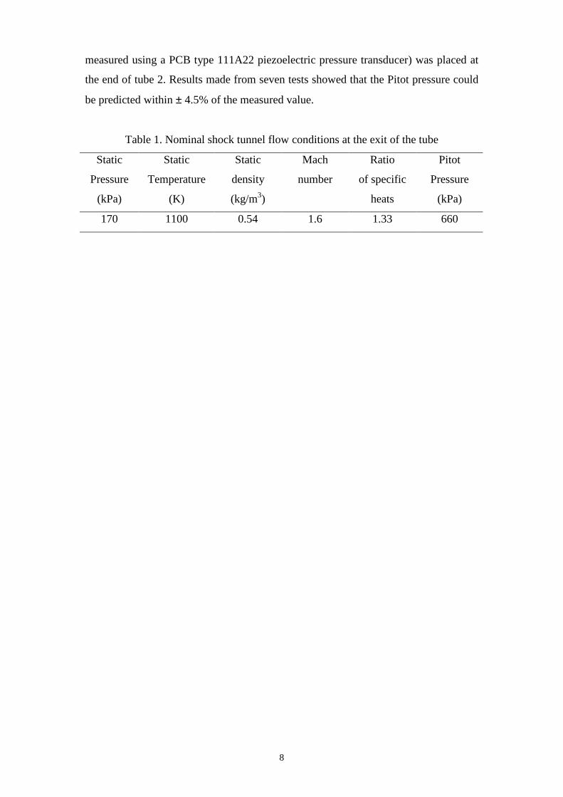
8
measured using a PCB type 111A22 piezoelectric pressure transducer) was placed at
the end of tube 2. Results made from seven tests showed that the Pitot pressure could
be predicted within ± 4.5% of the measured value.
Table 1. Nominal shock tunnel flow conditions at the exit of the tube
Static
Pressure
(kPa)
Static
Temperature
(K)
Static
density
(kg/m3)
Mach
number
Ratio
of specific
heats
Pitot
Pressure
(kPa)
170 1100 0.54 1.6 1.33 660
9
3. Comparison of results between different Pitot pressure measurement devices
Three different types of probes for measuring Pitot pressure have been used in the
present study. These include a Pitot probe with a piezoelectric pressure sensor as
detailed in Fig. 2, referred to as the X1 Pitot probe, a bar gauge of the design
presented by Sutcliffe [5] as detailed in Fig. 3, referred to as the Sutcliffe bar gauge,
and the new bar gauge of the present work shown in Fig. 4, referred to as the Chiu bar
gauge. For the tests presented in this section, the Chiu bar gauge had both a
semiconductor strain gauge and a piezoelectric film strain gauge installed on the
sensing bar. The details of these gauges are given in section 2.2. The test conditions
for the shots presented in this section are summarised in Appendix B.
In order to compare the performance of the different Pitot pressure probes, each was
tested in the X1 expansion tube. Due to the small size of the tunnel, it was not
possible to place more than one Pitot probe in the test flow for any one test. In
separate tests, each probe was placed at the same position, right at the exit plane of the
tunnel. The static pressure time history from the last pressure transducer mounted in
the wall of the acceleration tube, designated transducer at8, was recorded for each test
and was used to gauge the shot-to-shot variations in conditions. This pressure
transducer is 119 mm upstream of the exit of the tunnel. After each test, an averaged
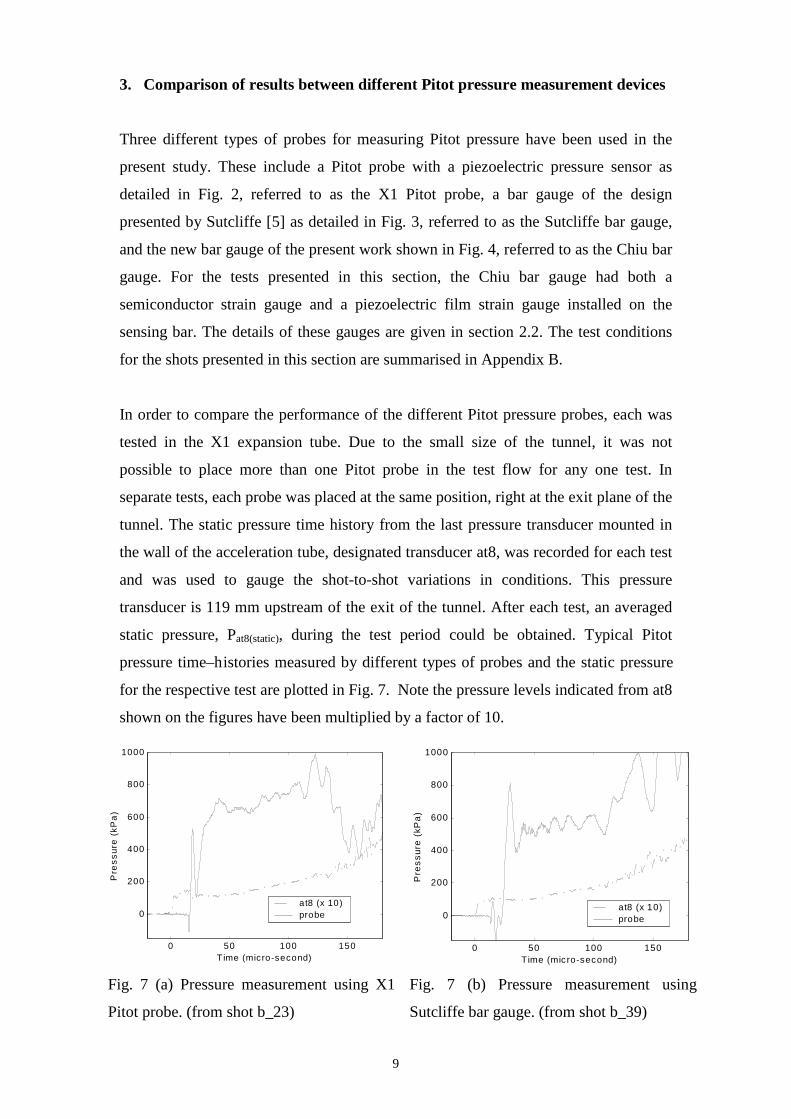
static pressure, Pat8(static), during the test period could be obtained. Typical Pitot
pressure time–histories measured by different types of probes and the static pressure
for the respective test are plotted in Fig. 7. Note the pressure levels indicated from at8
shown on the figures have been multiplied by a factor of 10.
000 505050 100100100 150150150
000
200200200
400400400
600600600
800800800
100010001000
Time (micro-second)Time (micro-second)Time (micro-second)
Pre
ss
ure
(kP
a)
Pre
ss
ure
(kP
a)
Pre
ss
ure
(kP
a)
at8 (x 10)at8 (x 10)at8 (x 10)probe probe probe
000 505050 100100100 150150150
000
200200200
400400400
600600600
800800800
100010001000
Time (micro-second)Time (micro-second)Time (micro-second)
Pre
ss
ure
(kP
a)
Pre
ss
ure
(kP
a)
Pre
ss
ure
(kP
a)
at8 (x 10)at8 (x 10)at8 (x 10)probe probe probe
Fig. 7 (a) Pressure measurement using X1
Pitot probe. (from shot b_23)
Fig. 7 (b) Pressure measurement using
Sutcliffe bar gauge. (from shot b_39)

10
0 50 100 150
-200
0
200
400
600
800
1000
Time (mic ro -second)
Pre
ss
ure
(k
Pa
)
at8 (x 10 ) semi-conduc to rfilm
Fig. 7 (c) Pressure measurement using Chiu bar gauge. (from shot s10_14)
By knowing the flow arriving time at at8, the distance between the location of at8 and
the exit plane of the tunnel (119 mm), the tunnel-recoil distance (25 mm) and the
respective flow speed for each shot, the time when the flow arrives at the tip of the
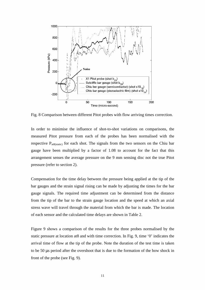
probe could be predicted. Figure 8 shows a comparison of results from the different
types of Pitot probes. For all tests, time ‘0’ indicates the time at which the flow arrives
at the tip of the probe.
From Fig. 8, two points are noted:
1) There are small shot-to-shot variations which result in different Pitot pressures for
the three shots.
2) The signals from the bar gauges do not rise immediately when the flow arrives at
the tip of the probe. This is because it takes some time for stress waves to
propagate from the tip of the probe to the location of the strain sensor. Note that
for the results from the Chiu bar gauge, the different distances from the tip of the
probe of the semiconductor strain gauge and the piezoelectric film gauge (15 mm
and 65 mm respectively) result in the rises in indicated pressure occurring at
different times.
11
Fig. 8 Comparison between different Pitot probes with flow arriving times correction.
In order to minimise the influence of shot-to-shot variations on comparisons, the
measured Pitot pressure from each of the probes has been normalised with the
respective Pat8(static) for each shot. The signals from the two sensors on the Chiu bar
gauge have been multiplied by a factor of 1.08 to account for the fact that this
arrangement senses the average pressure on the 9 mm sensing disc not the true Pitot
pressure (refer to section 2).
Compensation for the time delay between the pressure being applied at the tip of the
bar gauges and the strain signal rising can be made by adjusting the times for the bar
gauge signals. The required time adjustment can be determined from the distance
from the tip of the bar to the strain gauge location and the speed at which an axial
stress wave will t ravel through the material from which the bar is made. The location
of each sensor and the calculated time delays are shown in Table 2.
Figure 9 shows a comparison of the results for the three probes normalised by the
static pressure at location at8 and with time correction. In Fig. 9, time ‘0’ indicates the
arrival time of f low at the tip of the probe. Note the duration of the test time is taken
to be 50 µs period after the overshoot that is due to the formation of the bow shock in
front of the probe (see Fig. 9).

12
Table 2. Locations of strain sensors on each probe
Sensor Piezoelectric film
on Sutcli ffe bar gauge
Semiconductor
on Chiu bar gauge
Piezoelectric film
on Chiu bar gauge
Distance + (mm)
Time delay (µs)
15
4.5
15
4.5
65
19
+ Distance is measured from the tip of the probe.
Figure 9. Comparison between different types of Pitot probes with signals normalised
by the static pressure at location at8 and with time correction.
Several important points are drawn from the results shown in Fig. 7, Fig. 8 and Fig. 9.
It is apparent that all sensors are affected by noise at the start of the test. Note that all
gauges are affected by electrical interference that occurs when the flow arrives at the
tip of the probes (see the circle labelled ‘Noise’ in Fig. 8). This is attributed to
ionisation of the flow when the flow reaches high temperature in stagnation region
and has been observed in other high-enthalpy faciliti es [11]. The effect is different on
different types of sensors but always starts when the flow arrives at the tip of the
probe. It is apparent from the fact that the noise spike occurs at the same time on the
two sensors on the Chiu bar gauge that it is due to electrical interference and not a true
strain change. The source of this noise is addressed further in section 4.

13
Figure 9 shows that when the Pitot pressure signals are normalised by the average
pressure at at8, good agreement is obtained between the measurements from the X1
Pitot probe, the Sutliffe bar gauge and the semiconductor strain gauge on the Chiu bar
gauge. During the test time the results agree to within +/- 5%. Note however that the
signal from the piezoelectric film on the Chiu bar gauge indicates a significantly
lower level. It can be seen that the signal from this sensor does not return to zero after
the initial spike when the flow reaches the tip of the probe. Note that the amount of
this offset before and after the initial spike is close to 10 (PPitot / Pat8(static)) (see Fig. 9).
When the amount of the offset is added to the level indicated by the piezoelectric film
gauge, the signal level from the sensor becomes approximately equal to the level
indicated by the semiconductor strain gauge. Thus, in order to obtain an accurate
measurement using the piezoelectric film gauge, the amount of the offset due to the
initial spike must be taken into account. The semiconductor strain gauge signal does
not suffer from this offset effect. It is recommended that they be used in preference to
piezoelectric film sensors.
These results also show that that the influence of the noise spike can be reduced by
locating the semiconductor strain gauge further from the tip of the probe. Then by the
time the stress wave initiated by the arrival of flow at the probe tip reaches the strain
sensor, the noise spike will have already passed. Subsequent to these tests, Chiu bar
gauges were instrumented with only semiconductor strain gauges that were located 40
mm from the tip of the probes. (Note that the gauges were only 15 mm from the tip
for the probe used in test s10_14.) An example of a signal from one of the probes of
the final design is shown in Fig. 11(b).
Note that the result from the Sutcliffe bar gauge is nosier than those from the other
instruments during the test period. This suggests the sensing bar might have touched
the outer shielding cover during the test. (Refer to [4] for more details.)

14
4. Noise on bar gauge signals
This section addresses the source and effects of noise spikes that occurred regularly
on signals from the bar gauge measurements. Techniques to minimise the effects of
these noise spikes are also described. Note that the bar gauges used for measurements
in this section are detailed in section 2 and the test conditions for the shots presented
are summarised in Appendix B.
In order to investigate the noise on a bar gauge signal, consider an idealised response
of a gauge with a long bar in a pulsed flow (see Fig. 10). The plot shows the expected
ideal time history signal from a dynamic strain sensor due to a short period of a
constant force (due to a pulse of flow) acting on the front face of a uniform cylindrical
bar of infinite length. There should be no stress waves propagating down the bar
before the flow arrives (period 1). When the flow arrives (point 1), there would be a
step change in axial stress at the location of the strain gauge in response to the sudden
increase in force acting on the bar. The level of stress can be determined from the area
of the cross section of the bar and the level of the dynamic force applied to the front
face of the bar. This is then the average pressure on the front end of the bar. Then
there would be a period of constant strain (period 2) associated with the constant level
of force applied to the bar. When the force drops (point 2), the level of the strain
signal drops back to zero. (period 3)
Figure 10. Ideal time history trace when a constant force acts on a bar.

15
Now consider the flow produced in an impulse hypersonic facility. When a bar gauge
is placed in such a gas flow, the strain sensor would ideally produce a trace of the
form shown in Fig. 10. In the present experiments, there were some deviations from
this idealised form of signal. In particular some spikes occurred regularly on the strain
signals. Example signals from the present experiments are shown in Fig. 11. Signals
are shown for a piezoelectric film strain sensor (Fig. 11(a)) and for a semiconductor
strain sensor (Fig. 11(b)). The signals are presented in the form of average pressure
acting on the disc of the bar gauge, determined from the strain signal and the
calibration. Several features in the signals, not present in the ideal trace in Fig. 10, are
indicated.
Figure 11 (a). Sample trace of measured pressure from a bar with a piezoelectric film
gauge. Shot s8_30, bar gauge located 200 mm downstream from the exit of the tunnel.

16
Figure 11 (b). Sample trace of measured pressure from a bar with a semiconductor
strain gauge. Shot s13_21 bar gauge located 200 mm downstream from the exit of the
tunnel. 1 µs rise time DC strain amplifier used.
4.1 Identification of the sources of the spikes on strain sensors
In order to identify and study the causes of the spikes seen in the signals from the
strain sensors, a series of non-reflected shock tunnel tests (flows with supersonic
speeds, see section 2.1.2) and expansion tube tests (flows with hypervelocities) have
been performed. The non-reflected shock tunnel tests were performed so that effects
due to high enthalpy flows could be avoided. The total enthalpy of the test flows from
the shock tunnel tests (approximately 1.8 MJ/kg) would not be high enough to cause
ionisation of the flow in the bow shock formed in front of the bar gauges. In contrast,
because of the high enthalpy within the test flows from the expansion tube tests
(approximately 50 MJ/kg), ionisation effects could interfere with the strain signals.
A typical measured pressure time history from a shock tunnel test is illustrated in Fig.
12. In this test, both a piezoelectric film gauge and a semiconductor gauge were
placed on the same sensing bar. A 10 µs rise time strain gauge amplifier was used for
the semiconductor strain gauge. The first overshoot in the indicated pressure at the

17
start of the tests attributed to the formation of the bow shock in front of the bar gauge
(see circle 1). The second rise (at approximately 115 µs) is caused by the stress waves
reflected from the downstream end of the bar gauge (see circle 2). This time can be
calculated from the speed at which an axial wave travels along the bar, the length of
the bar and the location of the gauge. Note that the film gauge on the bar used in Fig.
12 was located downstream of the semiconductor gauge. It can be seen that the strain
increase due to the arrival of f low at the probe is detected earlier on the semiconductor
gauge and that the reflected pulse (circle 2) occurs last for this gauge. Thus, the useful
measuring test time for a bar gauge depends on the distance between the location of
the strain gauge and the end of the sensing bar. A longer distance gives a longer
measuring test time. The available measuring period is then defined as the time
between the stress wave’s first arrive at the strain gauge location and when the stress
waves reflected from the end of the bar return to the gauge location.
Figure 12. Typical signals from the shock tunnel test. (Shot ser10 S1)
The results from the shock tunnel tests can be used to identify that the spikes labelled
‘spike 2’ , in Fig. 11a and 11b are associated with the formation of the bow shock over
the bar. Also the increase in signal level at about 100 µs in Fig. 11b labelled ‘spike 4’ ,
is due to the stress waves reflected from the end of the sensing bar.

18
Note that the increase in signal level labelled ‘spikes 2’ and ‘spike 4’ in Fig. 11 and
12 are due to the aerodynamic forces acting on the sensing bars. Both spikes occurred
throughout the shock tunnel tests and the expansion tube tests. However the spikes
labelled ‘spike 1’ and ‘spike 3’ in Fig. 11 only occurred in the high enthalpy
expansion tube tests. This implies that spikes 1 and 3 are due to high temperature
effects.
As mentioned in section 2.1, the bar gauges are used to sense the stress waves
propagating down the sensing bar. The stress waves are generated by the aerodynamic
force acting on the front disc of the bar. Thus, before the flow hits the front disc, there
should be no stress waves propagating down the sensing bar. In the other words, the
level of the signals from the gauges should be zero. However, this is not the case
when following the traces of the signals in Fig. 11. There is a spike, labelled ‘spike 1’
in Figs. 11(a) and 11(b), that occurs before the flow arrives. In order to examine if
these spikes are due to noise caused by some form of electrical interference or a real
strain signal due to a force acting on the bar, a ‘dummy’ bar gauge was placed inside
the dump tank of the tunnel. The front disc of the dummy bar was removed and the
open end of the bar was sealed with a piece of brass shim. With such an arrangement,
the bar gauge will see no aerodynamic load and there should be no strain induced in
the bar and therefore no signal.
For shot s8_39, two probes were located a distance of 50 mm downstream of exit
plane of the acceleration tube. One probe was an active bar gauge with two
piezoelectric film strain sensors and the second probe was a dummy bar gauge as
described above. The dummy bar was instrumented with a single piezoelectric film.
The active probe was located 14 mm below the central-line of the test flow and the
dummy probe was located 56 mm above that probe. Figure 13 plots the signals
indicated by the three sensors on the two bars. The delay time between the signals
from the 1st gauge and the 2nd gauge is due to them being located at different distances
from the front disc (40 mm and 65 mm respectively). The dummy bar gauge does not
produce a null signal and it is clearly apparent that the phenomena labelled spikes 1
and 3 in Fig. 11(a) are also observed on this dummy bar gauge. It is shown in Fig. 13,
that spikes 1 and 3 were still observed on the dummy bar at the same time and of the
same magnitude. This confirmed that the spikes were noise caused by electrical
interference. Further, these spikes are also detected by both sensors on the active bar

19
gauge. Note that they occur at the same time on both these sensors. This provides
further evidence that the spikes are due to electrical interference.
Figure 13. Results from bar gauges (taken from s8_39)
It is proposed that both these noise spikes are caused by high temperature effects.
When a high speed gas flow is brought to rest (stagnated), the high temperatures that
result can cause the gas molecules to ionise [12]. This can lead to noise on signals
from instrumentation in expansion tubes and shock tunnels. If the noise occurs during
the test period, inaccurate readings can result.
For the present expansion tube experiments, the temperature of the stagnated N2 test
flow is estimated to be more than 20000 K (using EQSTATE [6]). Since N2 begins to
ionise above a temperature of 9000 K [12], ionisation is expected to occur when the
test flows of the present experiments are brought to rest. The time at which the flow
arrives at the front disc on the bar gauge coincides with the time of the spike
identified by circle 1 in Fig. 13. This occurs before the stress waves reach the
locations of the strain gauges. The time at which the noise identified by circle 2 in
Fig. 13 occurs coincides with the time when the slug of test gas reaches the end wall
of the dump tank. This will also cause the flow to stagnate. It is apparent from the
dummy bar in Fig. 13 that this leads to a large charge in the output signal from the

20
piezoelectric film strain gauge. Note here that the time between the flow reaching the
tip of the probe and the end of the dump tank decreases as the probe is moved further
downstream (see Fig. 20 (b) in [4]).
The effects of this noise are summarised as follows.
• For the piezoelectric film gauges, the level of the signal did not return to the
undisturbed level after the noise spike associated with the flow stagnating at the
tip of the probe. (Refer to Figs. 11, 13 and 14.) This results an offset in the zero
level of the signal before and after the spike. In order to obtain an accurate level of
the signal during the test window, this offset level has to be taken into account.
Note that the offset amount
• The noise spike associated with the flow stagnating at the end of the dump tank
had a much larger influence on the signal than did the noise spike associated with
the flow stagnating at the tip of the probe. (refer to Figs. 11, 13 and 14)
• The useful duration for pressure measurement was reduced as the bar was placed
further downstream from the exit plane. (refer to Fig. 20(b) in [4])
• Note that the noise associated with flow stagnating at the end of the dump tank
was not detected by the semiconductor gauges.
4.2 Minimising the effects of noise on the strain gauge signals
This section describes the improvements made to minimise the effects of noise due to
stagnation of the flow at the tip of the probe and at the end of the dump tank.
4.2.1. Position of strain gauges
The noise on the signal associated with the flow stagnating at the tip of the probe
could be separated from the signal due to a change in strain in the bar by placing the
gauge further from the front of the bar gauge. Because of the finite time taken for the
stress waves to travel from the front of the bar to the gauge location, moving the
21
gauge further down the bar allows the first spike to be separated in time from the
strain signal. Experimental results indicates that by placing the strain gauge 40 mm
from the front of the bar the effects of the first noise spike can be avoided and a 100
µs pressure measurement period can be obtained (Fig. 11(b)).
Note that for the piezoelectric film gauges, locating the gauge further down the bar
does not remove the effect of an offset in the zero level before and after the spike. The
second noise could not be decoupled from the true strain signal and the signal could
only be used for pressure measurement for times prior to arrival of this noise. This
occurred typically 100 µs after the flow exited from the end of the tunnel and
expanded into the dump tank (refer to Figure 20(b) in [4]). Thus, as the probe is
moved further downstream of the exit of the tunnel, the useful measurement period
decreases.
4.2.2. Use of semiconductor strain gauges
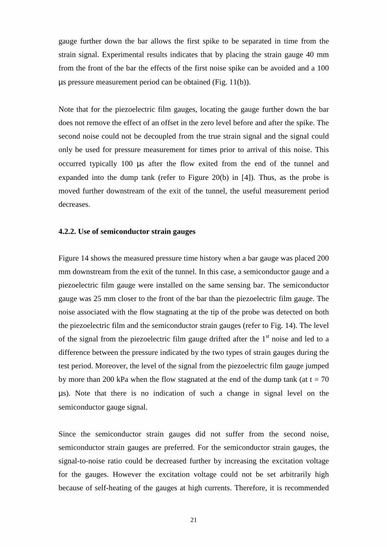
Figure 14 shows the measured pressure time history when a bar gauge was placed 200
mm downstream from the exit of the tunnel. In this case, a semiconductor gauge and a
piezoelectric film gauge were installed on the same sensing bar. The semiconductor
gauge was 25 mm closer to the front of the bar than the piezoelectric film gauge. The
noise associated with the flow stagnating at the tip of the probe was detected on both
the piezoelectric film and the semiconductor strain gauges (refer to Fig. 14). The level
of the signal from the piezoelectric film gauge drifted after the 1st noise and led to a
difference between the pressure indicated by the two types of strain gauges during the
test period. Moreover, the level of the signal from the piezoelectric film gauge jumped
by more than 200 kPa when the flow stagnated at the end of the dump tank (at t = 70
µs). Note that there is no indication of such a change in signal level on the
semiconductor gauge signal.
Since the semiconductor strain gauges did not suffer from the second noise,
semiconductor strain gauges are preferred. For the semiconductor strain gauges, the
signal-to-noise ratio could be decreased further by increasing the excitation voltage
for the gauges. However the excitation voltage could not be set arbitrarily high
because of self-heating of the gauges at high currents. Therefore, it is recommended

22
that the excitation voltage is set at 5 V while operating the tests and 0.2 V (the lowest
available voltage) after tests.
Figure 14. Pressure measurement results. (Shot s10_16. 1 µs strain gauge amplifier
used for semiconductor strain gauge)
4.2.3. Electrical isolation of the sensing bar
In order to minimise the effects of ionisation of the flow on the signal from the strain
gauges, the following steps were taken.
1. The sensing bar was electrically insulated from the outer shielding, by wrapping
the end of the sensing bar with electrical insulation tape before assembly.
2. A thin layer of paint was applied on the front disc.
This reduced, but did not eliminate, the first noise on the piezoelectric film strain
gauge signals. The improvement can be noticed by comparing the traces of the signals
obtained from the semiconductor strain gauges in Fig. 11 and Fig. 12. The noise level
of the 1st noise is reduced.

23
4.2.4. Contact between the disc and the sensing bar
A study by Chiu [13] showed that the propagation of stress waves can be affected by
the quality of joints between elements. Thus, the quality of signals from the Chiu bar
gauges will depend on the quality of the joint between the front disc and the sensing
bar. This subsection illustrates the signals obtained for bars with different qualities of
joints between the front disc and the sensing bar. The improvement that can be
achieved by attaching the disc to the sensing bar with LocTite (401) is then shown.
A series of experiments was completed to show the importance of the quality of the
contact surface between the front disc and the inner sensing bar of the Chiu bar gauge.
Experiments were performed using the straight-through non-reflected shock tunnel
method described in the section 2.3.2. Semiconductor strain gauges connected to 10
µs strain gauge amplifiers were used. The quality of the joint between the front disc
and the sensing bar is defined as follows.
• Tight – the front disc is screwed into the sensing bar by hand as tightly as possible
(finger-tight).
• Slightly tight – The disc is tightly attached to the sensing bar and then is
unscrewed by 45°.
• Loose – As for ‘slightly tight’ by the disc is unscrewed by 180°.
Figure 15 (a) shows the effects due to the different degrees of tightness. It can be seen
that a loose connection between the front disc and the sensing bar results a slow rise
time and large variations in the measurement signal during the 100 µs test window.
The result for the ‘slightly tight’ test also has a slow rise time but the variations during
the test window are not as large. A clear signal is obtained for the ‘tight’ disc. It is
recommended to ensure a ‘tight’ contact between the front disc and the sensing bar for
every test.
Tests were also performed with O-ring grease and Loctite (401) glue between the disc
and the sensing bar to see if this would improve the stress wave transmission. Three
tests were performed as follows.
• s11_30 – the front disc was finger tightened to the sensing bar.

24
• s11_31 – O-ring grease was applied onto the thread between the disc and the
sensing bar and the contact surfaces. Then the joint was tightened finger-tight.
• s11_39 – O-right grease was applied onto the thread between the disc and the
sensing bar and LocTite was applied onto the contact surfaces. The joint was then
tightened finger-tight.
The improvement from this application can be seen in the circled parts on Fig. 15(b).
The signal shown in Fig. 15(b)(a) indicates that a ‘bump’ occurs during the test
window even though the disc was tightened to the sensing bar. This is attributed to the
quality of the contact between the disc and the sensing bar. When this joint is not ideal
(eg. the surface of the disc is not exactly square to the surface of the sensing bar), it
leads to poor transmission of stress waves through the joint. By applying grease onto
the thread between the disc and the sensing bar and the contact surfaces, the quality of
signal transmission is improved (see Fig. 15(b)(b)). It can be seen that the method of
applying O-ring grease onto the thread between the disc and applying LocTite (401)
between the contact surfaces results a cleaner signal during the test window (see Fig.
15(b)(c)). It is recommended that O-ring grease be applied onto the thread between
the disc and the sensing bar and that LocTite (401) glue be applied to the contact
surfaces and then to tighten the joint finger tight when preparing a bar gauge.
Figure 15 (a). The effects on the pressure measurements due to the tightness between
the front disc and the sensing bar. (taken from s11_27, s11_28 and s11_29)

25
Figure 15 (b). Use LotTite to improve the stress waves transmission.
(taken from (a) s11_30, (b) s11_31 and (c) s11_39)
4.3. Summary
This section has demonstrated the methods used to identify noise on signals that
occurred in measurements with bar gauges. The formation of the bow shock in front
of the bar gauge results in an overshot in Pitot pressure before the test time. The finite
length of the sensing bar leads to a limitation of the period of time for which the bar
gauge can be used to indicate Pitot pressure. A noise spike was induced on the strain
signals when the high speed flow first stagnates at the front disc. The effects of this
noise can be minimised by locating the strain gauge further down the sensing bar (40
mm from the front end of the sensing bar was found to be suitable). Further noise was
generated when the slug of test gas stagnated at the back wall of the dump tank. The
effects of this could be eliminated by using semiconductor strain gauges. Thus,
semiconductor strain gauges are recommended as the strain sensors for measurements.
Electrically isolating the sensing bar from the tunnel leads to reduced noise. In
addition, by applying LocTite (401) to the contact surfaces between the front disc and
the sensing bar results an improvement in the signal transmission through the joint
and signals with reduced noise are achieved.

26
5. Uncertainties for Bar gauges
This section addresses the uncertainties in measurement of Pitot pressure using the
Chiu bar gauges. Since the accuracy of the measurements is affected by the
calibrations of the bar gauges, the uncertainties estimated in this section are based on
the results from the hammer and the shock tunnel calibrations described in section 2.
To analyse these errors, several uncertainties are considered. They are uncertainties in
disc dimensions, hammer calibrations, the relationship between average disc pressure
and Pitot pressure and steadiness of strain signals within the test window. The
methods used for the uncertainty analysis are based on those used in reference [14].
5.1 Sensitivity to the dimensions of the disc
As mentioned in the calibration section (section 2.3.1), the Chiu bar gauges are
calibrated by normalising the voltage output (V) indicated by the strain gauge with the
impact force (N) indicated by the impact hammer. In order to convert the sensitivity
of the bar gauge into V/kPa, the surface area of the disc attached to the bar gauge is
required. Thus, the accuracy of the calibration of the bar gauge is related to the disc
diameter (D). The discs are manufactured to a diameter of 9.0 mm within a tolerance
of ± 0.05 mm. After some shots the disc may abrade and it is estimated that the
diameter remains at 9.0 mm with an uncertainty of ± 0.1 mm. This leads to a ± 2.2%
in the uncertainty of the disc area (with a 95% confidence interval).
5.2 Uncertainties between average disc pressure and true Pitot pressure
A recent study of the relationship between the average disc pressure and the true Pitot
pressure has been completed by Mee et al. [15]. The report presents the results of a
computational fluid dynamic investigation into the average pressure on the end of a
flat-faced circular cylinder and how this varies in high speed flows. The MB_CNS
(multi-block, compressible flow, Navier-Stokes) code [16] was used to simulate the
flow conditions around a flat-faced cylinder. The results indicated that the ratio of
average pressure to the true Pitot pressure is approximately 0.93 ± 2% at the present
test conditions. This factor is similar to that obtained by Bourque [10] using Direct
Simulation Monte Carlo (DSMC) methods.

27
5.3 Uncertainty in strain signal variation
The uncertainty in strain signals from the bar gauge measurements during the
available test period is estimated using the results of 40 shock tunnel tests described in
section 2.3.2. A mean output voltage from the strain gauge is obtained during the test
period for each test, however, there are some variations in the signal about the mean
level during the test period. A standard deviation of these variations about the mean
was calculated for each test. With a 95% confidence interval, the uncertainty in the
strain signals over the test period due to noise and flow unsteadiness is ± 5.6% for the
conditions of the shock tunnel tests.
5.4 Uncertainty in the Pitot pressure measurements using the bar gauges
From the uncertainties described in sections 5.1, 5.2 and 5.3, the overall uncertainty in
measurement of Pitot pressure using the Chiu bar gauges is expressed as,
2222
2)(
∂∂+
∂∂+
∂∂+
∂∂= SSV
SSV
barADP
ADP
barDDV
DDV
barHC
HC
barbar X
X
XX
X
XX
X
XX
X
XX
where Xbar is the relative uncertainty in measurement of Pitot pressure using the bar
gauge, XHC is the relative uncertainty in hammer calibration (refer to section 2.3.1) of
the bar gauge, XDDV is the relative uncertainty in disc dimension variation, XADP is the
relative uncertainty in relationship between average disc pressure and true Pitot
pressure and XSSV is the relative uncertainty in steadiness of strain signal during the
test period. In this case, all partial derivations are equal to 1.0 so that,
2222 )()()()( SSVADPDDVHCbar XXXXX +++=
Using this, the uncertainty in measurement of Pitot pressures will be ± 7%.

28
6. Conclusion
This report has demonstrated the ability of the newly-designed bar gauges to measure
the Pitot pressures in impulsive flows. The modified bar gauges are re-useable and
can be used to measure Pitot pressures in low density flows. The response time is in
the order of 5 µs.
Experiments have be done to investigate the performance of the modified bar gauges
used for Pitot pressure measurements in impulsive flows. The overall uncertainty in
the measurement of disc average pressure is estimated to be ± 7% for flows with Pitot
pressures of order 600 kPa.
Two types of calibration methods for the bar gauges have been used. The accuracy of
the calibration using an impact hammer is estimated to be ± 3.5%. The uncertainty of
the calibration using the shock tube tests is related to the accuracy of the predicted
Pitot pressures. Results showed that the Pitot pressure could be predicted to within ±
4.5%.
A series of tests has been performed to investigate minimising the noise level on the
bar gauges. The effects from ionisation when the high enthalpy flow is stagnated at
the front disc can be avoided by locating the strain gauges 40 mm from the front end
of the bar. Semiconductor strain gauges are recommended in order to minimise the
effects of this noise. It is also recommended that vacuum grease be applied to the
thread on which the disc attaches to the stress bar and that LocTite (type 401) be used
to attach the front disc to the sensing bar. This improves the quality on the stress
wave transmission between the sensing disc and the stress bar.

29
7. Reference
1. Neely, A. J., Investigation of high enthalpy, Hypervelocity flows of ionisingArgon in an expansion tube’, The University of Queensland, Master thesis, 1991.
2. Wendt, M. N., Macrossan, M., Mee, D. and Jacobs, P. A., ‘Rarefied Gas DynamicFacility Experiments and Simulations’, Department of Mechanical Engineering,Departmental report 98/15, The University of Queensland, 1998.
3. Mudford, N. R., Stalker, R. J. and Shields, I., ‘Hypersonic nozzles for highenthalpy nonequilibrium flow’, Aeronautical Quarterly, May, 1980, pp 113-131.
4. Chiu, H. S., Mee, D. J. and Macrossan, M., ‘Development of a test facility forHigh speed Rarefied Flow’, Department of Mechanical Engineering,Departmental report 09/2000, The University of Queensland, 2000.
5. Sutcliffe, M., ‘The Use Of An Expansion Tube To Generate Carbone DioxideFlows Applicable To Martian Atmospheric Entry Simulation’, PhD thesis, TheUniversity of Queensland, 2000.
6. Neely, A. and Morgan, R., ‘The superorbital expansion tube concept, experimentand analysis’, Aero. Journal, March 1994, pp. 97-105.
7. Smith, A. L. and Mee D. J., ‘Dynamic strain measurement using piezoelectricpolymer film’, Journal of Strain Analysis, Vol. 31, No 6, 1996, pp. 463-465.
8. Anonymous, ‘Kulite semiconductor strain gauge manual’, Kulite SemiconductorProducts Inc. pp. 30-32, 1993.
9. Robinson, M., personal communication, 1999.
10. Bourque, B., ‘Development of a hypervelocity wind tunnel for rarefied flow’, B.E. thesis, The University of Queensland, 1999.
11. McIntyre, T. J., Lourel, I., Eichmann, T. N., Morgan, R. G., Jacobs, P. A., Bishop,A. I., ‘An experimental expansion tube study of the flow over a toroidal ballute’,Department of Mechanical Engineering, Departmental research report 2001/06,The University of Queensland, 2001.
12. Anderson, J. D., ‘Hypersonic and high temperature gas dynamics’, McGraw-Hill,1989.
13. Chiu, S., ‘Propagation of stress waves through screw joints’, B. E. thesis, TheUniversity of Queensland, 1996.
14. Mee, D. J., ‘Uncertainty analysis of conditions in the test section of the T4 shocktunnel’, Research Report 4/93, Department of Mechanical Engineering,Departmental research report 4/93, The University of Queensland, 1993.

30
15. Mee, D. J., Chiu, H. S. and Jacobs, P. A., ‘The average pressure on a flat-facedcircular cylinder in supersonic and hypersonic flows’, Department of MechanicalEngineering, Departmental research report 2004/01, The University ofQueensland, 2004.
16. Jacobs, P. A., ‘MB_CNS: A computer program for the simulation of transientcompressible flows; 1998 Update’, Department of Mechanical Engineering,Departmental Report 7/98, The University of Queensland, June 1998.

31
Appendix A
Manufacture and Instrumentation
of
the Bar Gauges

32
This section describes the manufacture of the components and the application of theinstrumentation for the new bar gauges. The workshop drawings for the componentsand an assembly drawing are shown in Fig. A1. Figure A1.b shows photographs ofthe manufactured components.
Figure A1.a The actual drawing for each component of a strain gauge bar (not to scale)
Figure A1.b Manufactured components A: Φ9 mm disc B: front outer shielding C: outer shielding D: connecting tube E: end cap F: sensing bar
A.1. Electrical circuit
The semiconductor strain gauges are installed by cementing them to the surface of thesensing bar. The cement used to apply the strain gauges is Micromeasurements M-Bond 200. The strain gauges are wired-up into a Wheatstone Bridge circuit in abending compensation arrangement (see Fig. A2). The Bridge is made using twosemiconductor strain gauges and two 120 Ω miniature resistors.
Figure A2 also shows the connections required for the Wheatsonte Bridge circuit for a25-pin connector used for the X1 instrumentation feed-through plate and a 9-pinconnector used for the strain gauge amplifier. The excitation voltage generated from a

33
strain gauge amplifier should be connected pins 11 and 5 on the 25-pin connector andbetween pins 1 and 5 on the 9-pin connector. A 1 m length of 4-core screened signalcable (eg. RS Components No. 367-347 cable) should be used to connect the bargauge to the connector. The 56 Ω resistor on the excitation line is installed tocompensate for loss of strain sensitivity with increasing temperature (see [8]).
Figure A2. Schematic of the Wheatsonte Bridge circuit and the connectors.
A 25-pin socket connector should be used for the bar gauges in X1 because theinstrumentation feed-through plate for X1 has only 25 pin connectors. If the resistanceof a particular semiconductor strain gauge is greater than 120 Ω, a suitable resistorshould be connected in parallel with that strain gauge to bring the resistance close to120 Ω. The earth screening on the 4-core cable should not be connected to any part ofthe bar to minimise the effects of electrical noise on the strain signals. After allconnections have been made, the cavity inside the 25-pin socket cover should be filledwith silastic to insulate and protect the connections.
A.2. Semi-conductor Strain Gauge information
Detailed information about Kulite semiconductor strain gauges is given in the manualprovided by Kulite [8]. Some important points are extracted and addressed below.
Gauge Code : ACP-120-300
' A' refers to gauges that are straight, with a bare silicon element, welded gold alloyleads (for higher temperature operation) and oriented axially to the gauge.
' C' : Gauge resistivity, controlled by dopant level
' P' : Gauge Factor Polarity, Positive
' 120' : Gauge resistance, 120 ohms
' 300' : Gauge length, 0.3"

34
In reference [8], the following is recommended:
“Cleaning of the specimen area before the installation is extremely important. Thesurface must be meticulously free of grease, oil , or wax. A grease or oil solvent suchas toluol should be used first, followed by MEK, acetone or trichlorethylene. Thesolvent must be clean. Although the gauges have been carefully cleaned beforepackaging, it is desirable to clean them again before mounting. Dip them in a cleansolvent and allow them to dry before bonding. Avoid touching or otherwisecontaminating the cementing surfaces before the gauge is installed.”
A.3. Installation for gauges
The step-by-step procedure used to install the gauges is as follows.
Step 1: Set the sensing bar in a small vice. See Fig. A3.Step 2: Measure the distance to where the strain gauge is to be located, and mark with
in pencil (about 40 mm from cap end is recommended). See Fig. A4.
Fig. A3. Step 1 Fig. A4. Step 2
Step 3: Spread Micromeasurements Catalyst-B on the area where the strain gauge is tobe attached. Wait for 1 minute until the Catalyst dries. See Fig. A5.
Step 4: Spread the Micromeasurements M-Bond 200 adhesive on the marked area.See Fig. A6.
Fig. A5. Step 3 Fig. A6. Step 4
35
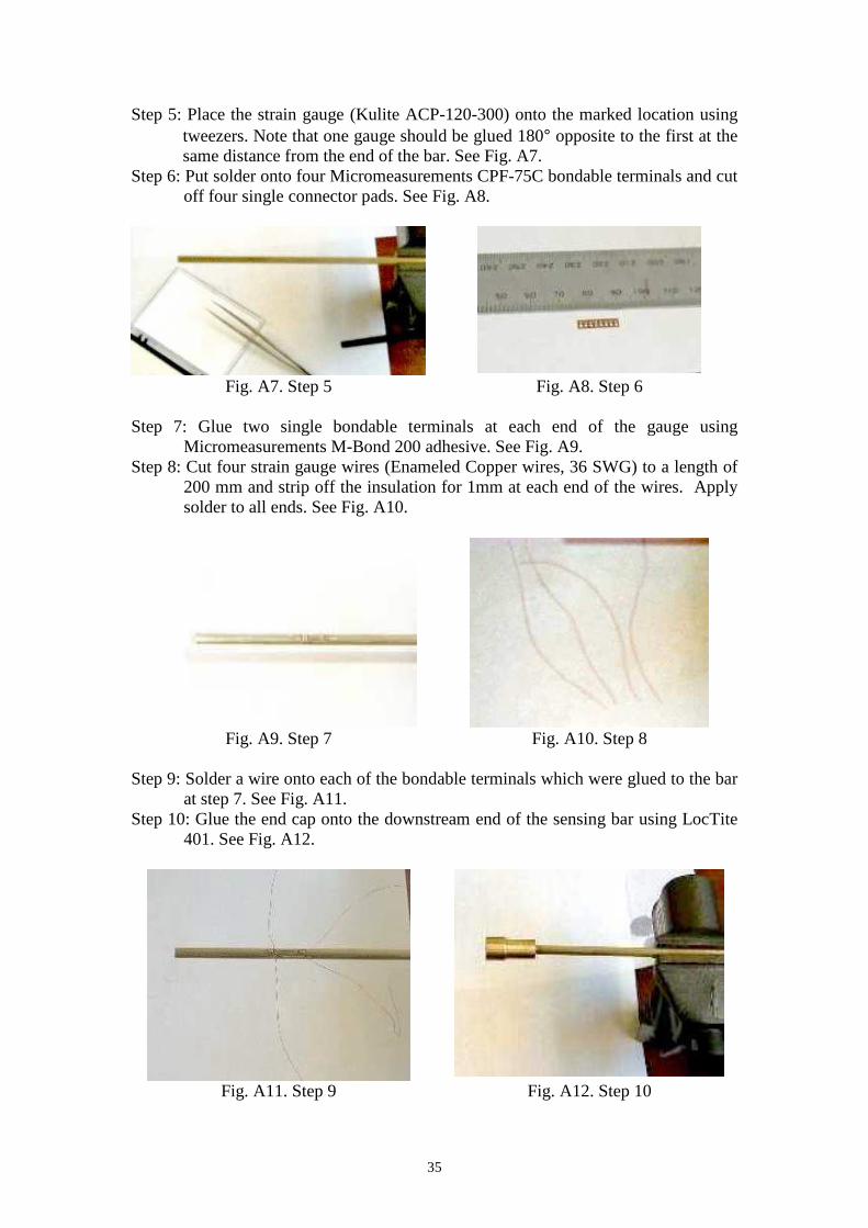
Step 5: Place the strain gauge (Kulite ACP-120-300) onto the marked location usingtweezers. Note that one gauge should be glued 180° opposite to the first at thesame distance from the end of the bar. See Fig. A7.
Step 6: Put solder onto four Micromeasurements CPF-75C bondable terminals and cutoff four single connector pads. See Fig. A8.
Fig. A7. Step 5 Fig. A8. Step 6
Step 7: Glue two single bondable terminals at each end of the gauge usingMicromeasurements M-Bond 200 adhesive. See Fig. A9.
Step 8: Cut four strain gauge wires (Enameled Copper wires, 36 SWG) to a length of200 mm and strip off the insulation for 1mm at each end of the wires. Applysolder to all ends. See Fig. A10.
Fig. A9. Step 7 Fig. A10. Step 8
Step 9: Solder a wire onto each of the bondable terminals which were glued to the barat step 7. See Fig. A11.
Step 10: Glue the end cap onto the downstream end of the sensing bar using LocTite401. See Fig. A12.
Fig. A11. Step 9 Fig. A12. Step 10

36
Step 11: Glue two single bondable terminals close to the end cap on the sensing bar.See Fig. A13.
Step 12: Solder a 120 Ω miniature resistor between the terminals attached at step 11(refer to A.1). See Fig. A14.
Fig. A13. Step 11 Fig. A14. Step 12
Step 13: Repeat steps 11 and 12 to attach another 120 Ω resistor 180° opposite to thefirst. See Fig. A15.
Step 14: Cut a 1 m length of 4-core screening cable (type RS Components, No. 367-347 cable). See Fig. A16.
Fig. A15. Step 13 Fig. A16. Step 14
Step 15: Strip off the outer shielding cover, 20mm in length, on one end of the 4-corecable. See Fig. A17.
Step 16: Separate the 4-core wires and the earth lead at the stripped end.See Fig. A18.
Fig. A17. Step 15 Fig. A18. Step 16

37
Step 17: Stripe off 5 mm of the insulation from the four wires. See Fig. A19.Step 18: Place solder on the appropriate pins of the connector (refer to Fig. A2).
See Fig. A20.
Fig. A19. Step 17 Fig. A20. Step 18
Step 19: Connect the four wires and the earth lead onto the connector prepared in step18. Refer to A2 for connection. See Fig. A21.
Step 20: Fill the cover for the connector with Silastic (silicone rubber). See Fig. A22.
Fig. 21. Step 19 Fig. A22. Step 20
Step 21: Place the connector prepared in step 19 into the cover. See Fig. A23.Step 22: Clip both covers together. See Fig. A24.
Fig. 23. Step 21 Fig. 24. Step 22

38
Step 23: Repeat steps 15 to 17 for the other end of the 4-core screening cable.However, on this end, strip off 50mm of the insulation and cut off the earthled. See Fig. A25.
Step 24: Connect these four wires to the bondable terminals prepared in step 12. Referto Fig. A2 for connections. See Fig. A26.
Fig. A25. Step 23 Fig. A26. Step 24
Step 25: Connect the four wires prepared in step 9 to the bondable terminals tocomplete the Wheatstone Bridge. See Fig. A27.
Step 26: Use Micromeasurements M-coat C (air-dry silicone rubber) to cover thestrain gauges, and the connector pads for the resistors. See Fig. A27.
Fig. A27. Step 27

39
Appendix BExperimental data by shots
This section summarises the test flow conditions for shots presented in this report.
Table B1. Results from the expansion tube tests
Shot StaticPressure
(kPa)
ShockSpeed(m/s)
Pitot +
Pressure(kPa)
Static +
Temperature(K)
Mach +
Number
b_23 11.7 8650 750 5800 5.3b_39 9.9 9800 555 5700 6.0s8_30 9.4 9750 540 5850 5.8s8_39 10.2 9650 820 6000 5.6s10_14 14.5 9400 740 5900 5.6s10_16 12.0 8700 680 5700 5.4s13_21 12.8 8750 500 5400 5.7
+ These are calculated results using TUBE [1].
Table B2 Results from the shock tunnel tests
Shot StaticPressure
(kPa)
ShockSpeed(m/s)
Pitot *
Pressure(kPa)
Static *
Temperature(K)
Mach *
Number
ser10 S1 173 1320 655 1060 1.6s11_27 173 1340 660 1090 1.6s11_28 173 1340 660 1090 1.6s11_29 174 1340 665 1095 1.6s11_30 172 1335 655 1090 1.6s11_31 171 1330 650 1080 1.6s11_39 174 1340 665 1095 1.6
* These are calculated results using EQSTATE [6].