1

Modelling Tourism Demand: A Dynamic

Linear AIDS Approach

GANG LI a, HAIYAN SONG

b, STEPHEN F. WITT b

a School of Management, University of Surrey, Guildford GU2 7XH, United Kingdom b School of Hotel and Tourism Management, The Hong Kong Polytechnic University,

Hung Hom, Kowloon, Hong Kong

INTRODUCTION

Tourism is one of the world’s largest industries and has experienced rapid growth

in many developed and developing nations over the last three decades. Decision-

makers in tourist destinations, especially those destinations where tourism is one of

the major sources of foreign exchange, have put much effort into trying to understand

the key determinants of demand for their tourism products and services in the hope of

formulating and implementing appropriate tourism policies and strategies. Many

empirical studies on tourism demand modelling and forecasting have been published

over the period, and these studies have undoubtedly proved useful for tourism

decision-makers. Detailed reviews of such studies can be found in Witt and Witt

(1995), Lim (1997) and Song and Witt (2000). Most of the empirical studies are based

on the single-equation approach, which suffers from specific limitations. Eadington

and Redman (1991) have noted that this approach is incapable of analysing the

interdependence of budget allocations to different consumer goods/services. For

example, in the tourism context, the decision-making involves making a choice

The linear almost ideal demand system (LAIDS), in both static and dynamic forms, is

examined in the context of international tourism demand. The superiority of the

dynamic error correction LAIDS compared to its static counterpart is demonstrated

in terms of both the acceptability of theoretical restrictions and forecasting accuracy,

using a data set on the expenditure of United Kingdom tourists in twenty-two Western

European countries. Both long-run and short-run demand elasticites are calculated.

The expenditure elasticities show that travelling to most major destinations in

Western Europe appears to be a luxury for UK tourists in the long run. The demand

for travel to these destinations by UK tourists is also likely to be more price elastic in

the long run than in the short run. The calculated cross-price elasticites suggest that

the substitution/complementarity effects vary from destination to destination.

Keywords: Tourism demand, linear almost ideal demand system (LAIDS), error

correction, demand elasticity, forecasting

2

among a group of alternative destinations. A price change in one destination may

influence tourists’ decisions on travelling to a number of alternative destinations, as

well as their expenditure in those destinations. However, lacking an explicit basis in

consumer demand theory, the single-equation methodology cannot adequately model

the influence of a change in tourism prices in a particular destination on the demand

for other destinations. Another limitation of the single-equation approach is that it

cannot be used to test the symmetry and adding-up hypotheses associated with

existing demand theories.

The system of equations approach initiated by Stone (1954) overcomes these

limitations. By including a group of equations (one for each consumer good) in the

system and estimating them simultaneously, this approach allows one to examine how

consumers choose bundles of goods in order to maximise their preference or utility

with budget constraints. In the tourism context, the system of equations approach can

help to analyse the impacts of relative prices in different destinations on tourists’

budget allocation, i.e., which destination to visit amongst a group of alternatives.

Moreover, since the cross-price elasticities associated with the estimated equations

within the system have a strong theoretical base, the interrelationships between

alternative destinations can be effectively evaluated. Hence it provides more reliable

information for policy evaluation than the single-equation alternatives.

Although there are a number of system modelling approaches available, the almost

ideal demand system (AIDS), introduced by Deaton and Muellbauer (1980), has been

the most commonly used method for analysing consumer behaviour as it has

considerable advantages over the others. For example, it gives an arbitrary first-order

approximation to any demand system; it has a flexible functional form and does not

impose any a priori restrictions on elasticities; it is easy to estimate and largely avoids

the need for non-linear estimation; the restrictions of homogeneity and symmetry can

be tested through linear restrictions on the parameters in the model; it is derived from

the consumer cost function corresponding to price-independent generalised

logarithmic (PIGLOG) consumer preferences, which permits an exact aggregation

over consumers without imposing identical preferences. As far as aggregate data are

concerned, a rational representative consumer is assumed to make the budgeting

allocation. Therefore, although the AIDS model is developed on the basis of

microeconomic theory, it can readily be generalised to the aggregate level (Edgerton

et al 1996).

Although the AIDS model has received considerable attention in food demand

analysis, the application of this approach to tourism demand studies is still relatively

rare. A thorough literature search has identified the following publications. O’Hagan

and Harrison (1984) examined American tourists’ expenditure in each of 16

individual destinations, while White (1985) divided the 16 destinations into 7 regions

and added a transportation equation into the demand system. Syriopoulos and Sinclair

(1993) and Papatheodorou (1999) studied the demand for Mediterranean tourism by

tourists from the US and various European countries. De Mello et al (2002)

introduced a three-equation system to examine the expenditure allocations of UK

tourists in France, Portugal and Spain. Divisekera (2003) applied AIDS models to

Japan, New Zealand, UK and US demands for tourism to Australia and chosen

alternative destinations. Lyssiotou (2001) specified a non-linear AIDS model to study

UK demand for tourism to US, Canada and 16 European countries. The lagged

dependent variable was included in the AIDS specification to capture the habit

persistence effect. However, a few neighbouring destinations were aggregated in this

3

study, thus the substitution and complementary effects between these individual

countries were not available. All of the above studies focus on tourists’ expenditure

allocation to different destinations, whereas Fujii et al (1985) investigated tourists’

expenditure on different consumer goods in a particular destination. Apart from

Lyssiotou (2001), the specifications of AIDS models in all the other studies are static

and can only give estimates of long-run demand elasticities. Although Lyssiotou

(2001) incorporated the lagged dependent variable into the model specification,

neither the long-run equilibrium relationship nor the short-term adjustment

mechanism has been examined. Unlike all the above studies, Durbarry and Sinclair

(2003) estimated an error correction AIDS in analysing the demand for tourism to

Italy, Spain and the UK by French residents. This is the first attempt to use the error

correction AIDS approach in tourism demand modelling and forecasting. However,

the error correction AIDS models in their study omitted all the short-run explanatory

variables due to their statistical insignificance. Thus, the tourists’ short-run behaviour

was not analysed in the study. Moreover, the forecasting performance of the dynamic

AIDS was not examined in their study. The present study uses the cointegration and

error correction approaches in the specification of the AIDS models, which allow a

full analysis of tourists’ dynamic behaviour. In other words, the responses of tourists

to price and expenditure changes in the long run and short run are examined

simultaneously. Furthermore, this dynamic AIDS model is expected to generate more

accurate forecasts than the conventional static AIDS model, especially in the short

run. This hypothesis is tested in Section 4.

THE MODELS

Static LAIDS

The static AIDS can be viewed as an extension of the Working-Leser model

(Working 1943; Leser 1963) in which the budget share for good i is related to the

logarithms of prices and total real expenditure in the following manner:

∑ ++=j

ijijii Pxbpaw )/log(logγ (1)

where wi is the budget share of the ith good, pj is the price of the jth good, x is total

expenditure on all goods in the system, P is the aggregate price index, x/P is real total

expenditure, and ia , ib and ijγ are the parameters that need to be estimated.

The aggregate price index P is defined as:

∑ ∑∑++=i i j

jiijii pppaP loglog2

1loglog 0 γα (2)

where 0a and iα are the parameters that need to be estimated.

Equation (2) shows that the relationship between the price index P and the prices

of individual goods is non-linear, which results in a complicated non-linear estimation

of the system. To linearise the relationship, Deaton and Muellbauer (1980) suggested

to replace the price index P with Stone’s price index (P*) which takes the form

4

∑=i

ii pwP log*log . The linear approximation of the AIDS model using this Stone’s

price index is termed the LAIDS. Deaton and Muellbauer (1980) found that such a

linear approximation works well when the individual prices in the system are

collinear.1 In tourism demand studies, the commonly used price variables are

consumer price indices (CPIs), which tend to be highly corelated especially amongst

the destinations in the same region such as Western Europe (see, for example,

O’Hagan and Harrison 1984). Therefore, the linear approximation of AIDS should be

more relevant to tourism demand.

To comply with the theoretical properties of demand theory, i.e. the budget

constraint and utility maximisation, the following restrictions are imposed on the

parameters in the AIDS model:

Adding-up restrictions: ∑=

=n

i

ia1

1, ∑=

=n

i

ij

1

0γ , and ∑=

=n

i

ib1

0 , which allows for all

budget shares to sum to unity;

Homogeneity: ∑ =j

ij 0γ , which is based on the assumption that a proportional

change in all prices and expenditure does not affect the quantities purchased. In other

words, the consumer does not exhibit money illusion;

Symmetry: jiij γγ = , which takes consistency of consumers’ choices into account;

Negativity: this requires the matrix of substitution effects to be negative

semidefinite. One subset of the negativity restriction implies that all the compensated

own price elasticities must be negative (Fujii et al 1985).

Researchers are very much interested in the demand elasticities. Due to the flexible

functional form of the LAIDS model, the elasticity analysis can be easily carried out.

The demand elasticities are calculated as functions of the estimated parameters, and

they have standard implications. The expenditure elasticity ( ixε ), which measures the

sensitivity of demand in response to changes in expenditure, is calculated

using iiix wb /1+=ε . The uncompensated own-price elasticity ( iiε ) and cross-price

elasticity ( ijε ) measure how a change in the price of one product affects the demand

for this product and other products with the total expenditure and other prices held

constant. They are given by 1/ −−= iiiiii bwλε and ijiiijij wwbw // −= λε ,

respectively. In the same way, the compensated price elasticities ( *

iiε and *

ijε ), which

measure the price effects on the demand assuming the real expenditure ( Px / ) is

constant (Pyo et al 1991), are calculated as 1/* −+= iiiiii wwγε and jiijij ww += /* γε .

In particular, the sign of the calculated *

ijε indicates the substitutability or

complementarity between the destinations under consideration (Edgerton et al 1996).

1 If prices are not collinear, the use of this linear approximation may cause inconsistencies in parameter

estimates. However, these inconsistencies are more serious in micro rather than aggregate data

(Pashardes 1993).

5

Error correction LAIDS

In the static LAIDS, which is also known as the long-run LAIDS model, it is

implicitly assumed that there is no difference between consumers’ short-run and long-

run behaviour, i.e. the consumers’ behaviour is always in “equilibrium”. However, in

reality, habit persistence, adjustment costs, imperfect information, incorrect

expectations and misinterpreted real price changes often prevent consumers from

adjusting their expenditure instantly to price and income changes (Anderson and

Blundell 1983). Therefore, until full adjustment takes place consumers are “out of

equilibrium”. This is one of the reasons why most static LAIDS models cannot satisfy

the theoretical restrictions (Duffy 2002). It is therefore necessary to augment the long-

run equilibrium relationship with a short-run adjustment mechanism. Moreover, the

static LAIDS pays no attention to the statistical properties of the data and the dynamic

specification arising from time series analysis. It is well known that most economic

data are non-stationary, and the presence of unit roots may invalidate the asymptotic

distribution of the estimators. Therefore traditional statistics such as t, F and R2 are

unreliable, and least squares estimation of the static LAIDS tends to be spurious

(Granger and Newbold 1974; Chambers 1993). Furthermore, the static LAIDS is

unlikely to generate accurate short-run forecasts (Chambers and Nowman 1997).

The concepts of CI and the ECM were first proposed by Engle and Granger (1987),

and have been widely used by researchers and practitioners in modelling and

forecasting macroeconomic activities over the last decade. The CI/ECM technique is

useful for the following reasons. First, policy makers and planners are often interested

in the long-run equilibrium relationship between economic variables, while marketers

are mainly concerned with the short-run disequilibrium behaviour of markets and

consumers. Engle and Granger (1987) showed that the long-run equilibrium

relationship can be conveniently examined using the CI technique, and the ECM

describes the short-run dynamic characteristics of economic activities. By

transforming the CI regression into an ECM, both the long-run equilibrium

relationship and short-run dynamics can be examined. Secondly, the spurious

regression problem will not occur if the variables in the regression are cointegrated.

Thirdly, the regressors in an ECM are almost orthogonal and this avoids the

occurrence of multicollinearity, which may otherwise be a serious problem in

econometric analysis (Syriopoulos 1995).

Before examining the CI relationship, all variables concerned need to be tested for

unit roots (or orders of integration). The Augmented Dickey-Fuller (ADF) (Dickey

and Fuller 1981) and Phillips-Perron (PP) (Phillips and Perron 1988) statistics can be

employed for this purpose. Once the orders of integration of the variables have been

identified, either the Engle and Granger (1987) two-stage approach or the Johansen

(1988) maximum likelihood approach can be used to test for the CI relationship

among the variables in the models (Song and Witt 2000).

Once the CI relationship between the dependent variables and the linear

combination of independent variables in the long-run LAIDS is confirmed, an ECM

of the LAIDS can be established and econometrically estimated with appropriate

algorithms. The ECM of the LAIDS (EC-LAIDS) used in this paper follows Ray

(1985) and Blanciforti et al (1986) and is given by:

11 *)/log(log −− +∆+∆+∆=∆ ∑ iti

j

ijijitii Pxbpww µλγδ (3)

6

where ∆ refers to the difference operator, and 1−itµ is the ECM term, which measures

the feedback effects, and is estimated from the corresponding CI equation. iδ and iλ

are the parameters that need to be estimated. The restrictions in the static LAIDS are

also applicable here.

Applications of the EC-LAIDS can be seen in the studies of demand for non-

durable goods, food and meat products, such as Balcombe and Davis (1996), Attfield

(1997), Karagiannis and Velentzas (1997), Karagiannis et al (2000) and Karagiannis

and Mergos (2002). Durbarry and Sinclair (2003) introduced this approach to tourism

demand analysis. However, due to insignificant coefficients, all of the short-run

independent variables were deleted from their EC-LAIDS model. With such a

restricted model, the different behaviours of tourists in the long-run and short-run

could not be investigated. Moreover, the forecasting performance of the EC-LAIDS

was ignored in their study. The current paper, therefore, fills in these gaps in the

tourism literature.

Model estimation and restriction tests

Since the sum of all expenditure shares in the LAIDS model is equal to unity, the

residuals variance-covariance matrix is singular. The usual solution is to delete an

equation from the system and estimate the remaining equations, and then calculate the

parameters in the deleted equation in accordance with the adding-up restrictions. The

LAIDS model is commonly estimated using Zellner’s (1962) iterative approach for

seemingly unrelated regressions (SUR) in most empirical demand studies and this

method is also employed in this paper.

With regard to restriction tests for homogeneity, symmetry and the joint test for

both homogeneity and symmetry, the conventional methods include the Wald test,

likelihood ratio test and Lagrange multiplier test. However, simulation experiments

have shown that these tests have considerable bias towards rejection of the null

hypothesis, especially when they are applied to large demand systems with relatively

few observations (Laitinen 1978; Meinser 1979; Bera et al 1981; Balcombe and Davis

1996). Therefore, this study applies two sample-size-corrected statistics (see

Appendix 1) developed by Court (1968) and Deaton (1974) to avoid the over-

rejection of the null hypotheses.

EMPIRICAL RESULTS

The data

Both the static and EC-LAIDS models are estimated using data on the demand for

tourism to Western Europe by United Kingdom residents. There are twenty-two

destinations involved: Austria, Belgium, Cyprus, Denmark, Finland, France,

Germany, Gibraltar, Greece, Iceland, Irish Republic, Italy, Luxembourg, Malta,

Netherlands, Norway, Portugal, Spain, Sweden, Switzerland, Turkey and former

Yugoslavia. Western Europe is the most popular destination area for UK residents,

with tourist spending in this region accounting for 14.8 billion pounds in 2000, which

is 61.1% of the total demand. Within this area, France, Spain, Italy, Greece and

Portugal are the major destinations, and tourist spending in these five countries

7

accounts for more than 50% of the total in the twenty-two Western European

destinations (68.6% in 2000) (see Figure 1). Therefore, this study focuses on these

five destinations, with the other seventeen aggregated to a single group as Others.

FIGURE 1

SHARES OF UK TOURIST SPENDING IN WESTERN EUROPEAN COUNTRIES

(2000)

France

21.6%

Greece

7.3%

Italy

7.8%

Portugal

4.0%

Spain

27.9%Others

31.4%

The prices employed here are relative (or effective) prices, calculated by dividing

the price2 of each destination by that of the UK, adjusted by the appropriate exchange

rates. The aggregated price for the Others group takes the form of Stone’s price index.

All the prices are normalised to unity at the point of the base year (1995). Although

the expenditure data relate to all travelling purposes, they are highly correlated with

the expenditure data on holidays, as pleasure travel has been dominating the tourism

in the key destinations within the whole region concerned (see Table 1). Therefore,

the results of the estimated LAIDS model can reflect the characteristics of the

pleasure travel. The per capita expenditure is calculated and used in the model

estimation in order to account for the effect of population size changes over time. In

this empirical study, a three-stage budgeting process is followed. It is assumed that

tourists first allocate their consumption expenditure between total tourism

consumption and consumption of other goods and services. In the second stage,

tourists allocate their expenditure between tourism in Western Europe and in other

regions. In the last stage, tourists make their decisions among the alternative

destinations in Western Europe. The LAIDS models are applied to the last stage of

tourism expenditure allocation.

TABLE 1

RELATIONSHIPS BETWEEN TOURIST EXPENDITURE FOR HOLIDAYS AND

FOR ALL PURPOSES (1995-2001)

France Greece Italy Portugal Spain

Western

Europe

2 Most empirical studies on tourism demand use CPI as a proxy for the tourism price. Econometric

evidence has shown that the use of this proxy does not cause major conceptual or econometric

distortions (Witt and Witt 1992).

8

Correlation

Coefficient 0.97 1.00 0.96 0.99 1.00 0.99

Average

proportion (%) 64.3 91.8 67.3 88.3 90.4 70.6

The data on prices, exchange rates and population are collected from the

International Financial Statistical Yearbook (International Monetary Fund, various

issues), and the expenditure data are collected from Travel Trends (Office for

National Statistics, UK, various issues). The data set covers the period 1972-2000.

Model estimation

The ADF test for unit roots suggests that all the variables in the long-run LAIDS

are I(1), and the long-run equilibrium relationships cannot be rejected by the Engle-

Granger approach at the 5% significance level in any case.3 Therefore, the

unrestricted long-run static LAIDS models are estimated using the iterative SUR

method. With regard to the dynamic LAIDS, the Engle and Granger two-step

approach is employed for estimating CI regressions. The residuals from these

regressions are calculated and incorporated into Equation (3), and then the

unrestricted EC-LAIDS is estimated. The estimates are shown in Tables 2 and 3.

The estimated parameters iδ in the EC-LAIDS are all significantly different from

zero except in the Italian equation, which indicates that habit persistence plays an

important role in UK tourists’ decision-making process. In other words, the previous

distribution of tourism expenditure in different destinations influences UK tourists’

current decision on destination choice. The coefficients of error correction terms are

all statistically significant at the 1% level and correctly signed, suggesting that any

deviations of tourist spending from the long-run equilibrium are dynamically

corrected, and hence the specification of a dynamic LAIDS is appropriate.

3 The results are not presented due to space constraints, but are available from the authors upon request.

9

TABLE 2

ESTIMATES OF THE UNRESTRICTED STATIC LAIDS

France Greece Italy Portugal Spain

ia 0.176

(10.887) 0.024

(1.884) 0.116 (13.889)

-0.001

(-0.148) 0.142 (5.669)

1iγ -0.068

(-1.143) 0.057

(1.190) 0.038

(1.249) -0.007

(-0.291) 0.132

(1.429)

2iγ -0.111

(-2.104) -0.129 (-3.032)

0.068 (2.496)

0.008

(0.360) 0.064

(0.774)

3iγ -0.140 (-4.624)

-0.047 (-1.926)

-0.021

(-1.314) 0.050 (4.001)

0.094 (1.995)

4iγ 0.128 (3.176)

-0.039

(-1.196) -0.047 (-2.260)

-0.032

(-1.963) -0.108

(-1.727)

5iγ 0.181 (5.305)

0.074 (2.693)

-0.024

(-1.340) 0.020

(1.463) -0.270

(-5.101)

6iγ -0.096

(-1.414) 0.047

(0.862) -0.058

(-1.661) -0.019

(-0.678) 0.225 (2.128)

ib 0.007 (1.974)

0.009 (3.270)

-0.009 (-4.934)

0.008 (5.686)

0.027

(4.899)

2R 0.895 0.792 0.826 0.849 0.561

DW 2.24 1.31 1.66 1.80 2.21

Notes: the estimates in bold type are significant at the 5% significance level. Values in parentheses are

asymptotic t-statistics.

10

TABLE 3

ESTIMATES OF THE UNRESTRICTED EC-LAIDS

France Greece Italy Portugal Spain

iδ 0.156 (2.330)

0.177 (2.048)

0.125 (1.631)

0.342 (2.293)

0.331 (4.905)

1iγ -0.028 (-0.832)

0.101 (4.042)

0.049 (2.250)

-0.001 (-0.041)

0.108 (1.724)

2iγ -0.065 (-1.725)

-0.007 (-0.236)

0.024 (1.010)

0.054 (2.457)

-0.036 (-0.506)

3iγ -0.073 (-2.514)

-0.033 (-1.246)

-0.005 (-0.293)

0.061 (3.255)

0.063 (1.156)

4iγ 0.093 (2.687)

-0.058 (-1.800)

-0.059 (-2.685)

-0.035 (-1.738)

-0.064 (-0.996)

5iγ 0.029 (0.910)

0.021 (0.691)

-0.006 (-0.300)

-0.008 (-0.442)

-0.101 (-1.712)

6iγ -0.050 (-1.106)

-0.009 (-1.029)

-0.072 (-2.516)

-0.027 (-1.143)

0.211 (2.615)

ib 0.007 (0.633)

0.011 (1.103)

-0.015 (-2.200)

0.009 (1.501)

0.043 (2.251)

iλ -1.227 (-12.278)

-1.053 (-9.465)

-1.144 (-9.563)

-1.512 (-6.924)

-1.493 (-14.660)

2R 0.792 0.619 0.560 0.503 0.725

DW 1.74 1.68 1.79 1.88 1.79

Notes: same as Table 2.

With regard to the restriction tests, the EC-LAIDS passes all the tests at the 5% level,

while the static LAIDS fails the symmetry test and the joint tests for both

homogeneity and symmetry. It indicates that ignoring the dynamic adjustment is

likely to result in mis-specification of the functional form and violation of demand

theory. Since the imposition of these restrictions helps to reduce the number of

parameters to be estimated and increase the degrees of freedom, the homogeneity and

symmetry restricted static LAIDS and EC-LAIDS are both estimated and used for

elasticity analysis. The results are presented in Tables 5 and 6.

11

TABLE 4

RESTRICTION TESTS

Homogeneity Symmetry Homogeneity and symmetry

T1 T2 T1 T2 T1 T2

Static LAIDS 2.300** 11.512* 3.342 33.421 3.166 47.483

EC-LAIDS 1.685** 8.428** 1.617** 16.174** 1.634** 24.517**

Note: * and ** denote acceptance at the 1% and 5% significance levels, respectively.

TABLE 5

ESTIMATES OF THE HOMOGENEITY AND SYMMETRY RESTRICTED

STATIC LAIDS

France Greece Italy Portugal Spain

ia 0.230

(1.598)

-0.001

(-0.076) 0.133 (10.551)

-0.002

(-0.350) 0.210 (8.640)

1iγ -0.057

(-1.088)

0.017

(0.730) -0.038

(-1.660)

-0.003

(-0.188) 0.155 (3.767)

2iγ 0.017

(0.730)

-0.149

(-6.780)

-0.016

(-1.065)

-0.023

(-1.920)

0.002

(0.097)

3iγ -0.038

(-1.660)

-0.016

(-1.065)

0.003

(0.138)

0.030

(0.138) -0.043 (-1.720)

4iγ -0.003

(-0.188) -0.023

(-1.920)

0.030

(0.138)

-0.013

(-1.250)

-0.001

(-0.039)

5iγ 0.155

(3.767)

0.002

(0.097) -0.043

(-1.720)

-0.001

(-0.039) -0.201 (-3.247)

ib 0.016 (4.374)

0.014 (6.334)

-0.008 (-6.994)

0.008 (2.794)

0.014 (2.795)

2R 0.812 0.716 0.542 0.810 0.272

DW 1.347 1.303 0.849 1.484 1.344

Notes: same as Table 2.

12

TABLE 6

ESTIMATES OF THE HOMOGENEITY AND SYMMETRY RESTRICTED EC-

LAIDS

France Greece Italy Portugal Spain

iδ 0.114

(1.349)

0.060

(0.060)

0.156

(1.018)

0.319

(2.043) 0.262

(2.841)

1iγ 0.052

(1.591)

0.034

(1.555)

-0.013

(-0.727)

-0.021

(-1.359) 0.091

(2.535)

2iγ 0.034

(1.555) -0.071

(-2.726) -0.043

(-2.516)

0.018

(1.201)

-0.026

(-0.089)

3iγ -0.013

(-0.727) -0.043

(-2.516)

0.022

(0.994) 0.024

(2.000)

-0.008

(-0.288)

4iγ -0.021

(-1.359)

0.018

(1.201) 0.024

(2.000)

-0.003

(-0.231)

-0.030

(-1.652)

5iγ 0.091

(2.535)

-0.026

(-0.089)

-0.008

(-0.288)

-0.030

(-1.652) -0.160

(-2.410)

ib 0.022

(1.784)

0.014

(1.600)

-0.000

(-0.030)

0.002

(0.346)

0.010

(0.505)

iλ -1.048

(-8.169) -1.036

(-8.310) -1.012

(-4.583) -1.331

(-6.182) -1.241

(-8.565)

2R 0.539 0.472 0.105 0.292 0.569

DW 1.87 1.37 1.62 1.42 2.15

Notes: same as Table 2.

Demand elasticities

The long-run and short-run expenditure and price elasticities are calculated in

terms of the homogeneity and symmetry restricted systems, with iw and jw being

replaced by the average budget shares iw and jw , respectively. The calculated

elasticites are given in Tables 7 and 8 and they are also compared with those

published in previous studies.4

With respect to expenditure elasticities, the values are greater than unity no matter

whether the long run or short term is concerned, the only exception being Italy, where

the long-run elasticity is slightly lower than one. This suggests that travelling to the

major Western European countries is generally regarded as a luxury by UK tourists.

Compared with previous studies, the closest results can be found in expenditure

elasticities for Spain, with three out of four cases being aligned with our conclusion.

4 Since the deleted equation does not refer to any specific destination, the analysis of its elasticities is

meaningless and therefore is excluded from this study.

13

TABLE 7

EXPENDITURE ELASTICITIES: CALCULATED AND PREVIOUS

LITERATURE

Long-run Short-run L1 L2 L3_1 L3_2

France 1.09 1.12 0.63 0.81

Greece 1.20 1.20 1.05 0.80

Italy 0.90 1.00 0.88 1.05

Portugal 1.24 1.05 1.58 0.04 0.82 0.95

Spain 1.06 1.04 0.90 1.15 1.20 1.15

Notes: L1 denotes the study by Syriopoulos and Sinclair (1993), L2 by Papatheodorou (1999) and L3

by De Mello et al (2002). The whole sample is separated into 2 periods in L3, denoted as L3_1

and L3_2, respectively.

With regard to the own-price elasticities, all of the values are negative, in line with

demand theory. Since there is no significant difference between the uncompensated

and compensated price elasticities, only the compensated elasticities are reported.

TABLE 8

COMPENSATED OWN-PRICE ELASTICITIES: CALCULATED AND

PREVIOUS LITERATURE

Long-run Short-run L1 L2 L3_1 L3_2

France -1.17 -0.53 -1.76 -1.54

Greece -2.75 -1.91 -2.54 -0.93

Italy -0.93 -0.65 -1.24 -0.77

Portugal -1.16 -1.05 -2.69 -2.85 -2.16 -1.71

Spain -1.52 -1.32 -0.72 -0.65 -1.26 -1.40

Notes: same as Table 7.

Comparing the long-run elasticities with the short-run elasticities, it can be seen

that the long-run elasticites are generally greater than the short-run counterparts in

terms of the absolute magnitude, and it is the most evident in the cases of Greece and

France. This implies that in the long run tourists are more flexible in response to price

changes. In the short run, due to various reasons such as information asymmetry and

bounded rationality, tourists cannot fully adjust their behaviours when the price

change occurs. This conclusion is consistent with demand theory. Comparing the

magnitude of elasticities across destinations, UK tourists seem to be the most sensitive

to price variations in Greece, while the demand for tourism to Italy appears to be the

least price elastic. These results hold regardless of whether the long run or short run is

considered.

As far as the cross-price elasticities are concerned, the calculated results in both the

long run and short run are reported in Table 9, along with the corresponding results

14

from previous studies. In order to provide robust results, two criteria are followed to

select elasticities for examination, that is, the statistical significance in at least one of

the long-run and short-run elasticities and consistency of signs between long-run and

short-run elasticities. Compared with the previous literature, consistent substitution

effects can be found in the following pairs of destinations: France and Spain (same as

the results obtained by De Mello et al 2002 and Papatheodorou 1999), and Italy and

Portugal (same as Papatheodorou 1999). The substitutability between the pairs of

destinations is associated with their similar geographic features and cultural

backgrounds. Therefore, if tourism prices in one destination (e.g. France) increase,

tourists are likely to choose to go to the competing destination (e.g. Spain). However,

the results show that the degree of substitution between the two destinations is

different. For example, in the long run, if the prices in Spain increase by 1%, the

demand for France will increase by 1.15%. On the other hand, if the prices in France

increase by 1%, the demand for Spain will increase by only 0.77%. This indicates that

France has gained more competitiveness over Spain in attracting UK tourists’

expenditure. In addition to the substitution effect, the complementary effect is also

identified between Greece and Italy, which is in line with the results of Papatheodorou

(1999) and Syriopoulos and Sinclair (1993). The complementary effect occurs when

UK tourists take multiple-destination trips, i.e. the voyage effect holds (see

Papatheodorou 1999). A new outcome that has not been explored before refers to the

substitutability between France and Greece, especially in the short run. With respect

to the magnitudes of the elasticities, the values are lower than unity in terms of

absolute values with only one exception. Comparing with the own-price elasticities,

the cross-price elasticities show that the demand for tourism in a destination by UK

residents is much less sensitive to price changes in the alternative destinations. For

example, in terms of UK’s long-run demand for Spanish tourism, a 1% increase in

Spanish prices would lead to a 1.52% decrease in demand for Spanish tourism, while

the price changes in Greece, Italy and Portugal would not result in significant changes

in the demand for Spain. It implies that other factors beyond prices may play more

important roles in the competition between tourism products of different destinations.

Comparing various demand elasticities in this study with those in the previous

literature, it is common to see discrepancies, which possibly result from differences in

the groupings of destination countries (White 1985), estimation methods, sample

periods, definitions of the variables, budget shares ( ini ww / ) used for estimating

elasticities, and so on.

15

TABLE 9

COMPENSATED CROSS-PRICE ELASTICITIES: CALCULATED AND

PREVIOUS LITERATURE

France Greece Italy Portugal Spain

L1

L2

France 0.09 1.45 L3_2

0.19 -0.16 0.08 1.15 Static LAIDS

0.26 0.01 -0.08 0.78 EC-LAIDS

-0.23 0.56 1.22 L1

-0.98 1.06 1.16 L2

Greece L3_2

0.48 -0.03 -0.43 0.23 Static LAIDS

0.65 -0.51 0.29 -0.09 EC-LAIDS

-0.04 -0.83 0.41 L1

0.25 1.09 L2

Italy L3_2

-0.35 -0.03 0.33 -0.11 Static LAIDS

0.01 -0.46 0.34 0.18 EC-LAIDS

0.53 -4.40 4.08 L1

L2

Portugal 0.44 1.27 L3_2

0.35 -0.80 0.69 -0.05 Static LAIDS

-0.35 0.53 0.71 -0.50 EC-LAIDS

0.20 0.37 0.70 L1

L2

Spain 1.73 0.23 L3_2

0.77 0.06 -0.03 -0.01 Static LAIDS

0.52 -0.02 0.05 -0.07 EC-LAIDS

Notes: same as Tables 2, 7 and 8.

FORECASTING PERFORMANCE

Forecasting ability is an important aspect of evaluating the performance of an

econometric model. Forecasting tourism market shares and their relative changes

amongst the competing destinations is very important for destination management.

Many published studies on tourism forecasting show that the demand for tourism has

always been growing over time. But in a demand system, when some destinations are

predicted to gain more market shares, the others must suffer from the loss of their

relative competitiveness. Therefore, accurate market share predictions should provide

the destination government and tourism organisations with useful information for

competitiveness analysis and strategy formulation. This is an additional advantage of

16

the system of equations models, in particular the AIDS model, over the single-

equation approach. On account of the importance of market share forecasting, it is

necessary to evaluate the forecasting performance of the static and dynamic LAIDS.

Since the static LAIDS does not include any lagged variables, only one-year ahead

forecasts are comparable with those generated by the EC-LAIDS. Due to the failure to

pass the symmetry restriction test, the static symmetry-restricted LAIDS suffers from

misspecification, hence we use the unrestricted LAIDS to illustrate the difference in

forecast performance between the static and dynamic systems.

Before conducting forecasting tests, it is necessary to examine parameter stability

between the estimating period (1972-1996) and forecasting period (1997-2000). In

this study, the statistic proposed by Anderson and Mizon (1983) (see Appendix 2) is

utilised. The calculated statistics for both the static and EC-LAIDS models are less

than the critical value at the 5% significance level, indicating that there is no evidence

of parameter changes over the forecasting period, so the models concerned are

suitable for generating forecasts.

Both the static and dynamic unrestricted systems are re-estimated, first using the

observations from 1972 up to 1996, and then one more observation being added each

time, until the observations up to 1999 are used. Hence 4 one-year-ahead forecasts are

obtained for each destination, and 20 for the whole system. The forecasts generated by

the EC-LAIDS refer to differenced variables, which are then transformed into levels

variables in order to compare the results with those from the static LAIDS. The

comparisons are based on both individual equations (destinations) and the whole

system (region). The mean absolute percentage error (MAPE) and the root mean

square percentage error (RMSPE) are considered for both destination-specific and

system-specific comparisons of forecasting accuracy (Witt and Witt, 1992). The

results presented in Table 10 show that the EC-LAIDS always outperforms the static

LAIDS, no matter which destination is concerned, and, moreover, the EC-LAIDS is

41.5% and 48.4% more accurate than the static LAIDS in general, judged by the

MAPE and RMSPE, respectively. This result is not surprising, as the EC-LAIDS

incorporates the dynamic correction mechanism, and therefore tends to capture the

short-term variations more precisely. The similar result can also be found in

Chambers and Nowman (1997).

TABLE 10

FORECASTING ACCURACY COMPARISON BETWEEN STATIC AND

DYNAMIC UNRESTRICTED LAIDS

Static LAIDS EC-LAIDS Destination

MAPE RMSPE MAPE RMSPE

France 0.032 0.051 0.020 0.022

Greece 0.261 0.333 0.130 0.159

Italy 0.105 0.116 0.063 0.072

Portugal 0.153 0.171 0.098 0.099

Spain 0.023 0.026 0.024 0.033

Whole system 0.115 0.177 0.067 0.091

17

CONCLUDING REMARKS

In this study, the UK demand for tourism in Western Europe has been examined

using both the long-run static and the short-run EC-LAIDS models. Five destinations

are considered in this study: France, Greece, Italy, Portugal and Spain. The tests for

homogeneity and symmetry suggest that the dynamic version of the LAIDS satisfies

demand theory well, and that the short-run adjustment should not be ignored when

examining the demand for Western European tourism by UK residents. Various

elasticities have been calculated and the results provide a basis for tourism

policymaking in these destinations.

The calculated expenditure elasticities show that travel to most major destinations

in Western Europe appears to be a luxury for UK tourists in the long run. However, a

change in total tourist expenditure tends to have different influences on the demand

for alternative destinations. This indicates different positions of these destinations in

attracting the demand their tourism by UK residents (measured by per capita

expenditure). Portugal and Greece appear to benefit more from the increase in UK

tourists’ expenditure in the booming period while they may suffer more from the

economic recession in the UK. Hence it is important for Portugal and Greece to

closely monitor the economic cycles in the UK.

As far as the own-price elasticities are concerned, UK tourists are more sensitive to

price changes in the destinations in the long run than in the short term. The demand

for outbound UK tourism is most sensitive to price changes in Greece and least

sensitive to price changes in Italy. For the relatively price-elastic destinations, a

careful control in tourism prices relative to those in neighbouring counties would

benefit the growth of the tourism industry, which in turn would bring more foreign

exchange earnings to the destinations. With regard to the private sectors, it should be

noted that reducing prices is not necessarily the appropriate strategy to gain the

competitiveness against the rivals, because it may cause retaliatory measures.

The cross-price elasticities indicate that France and Spain are likely to be

substitutes in the minds of UK tourists, and also Italy and Portugal, and France and

Greece. Having been aware of their strongest competitors, these destinations should

keep a keen eye on their competitors’ actions in tourism product promotion, and carry

out quick counteracting strategies in response. To some extent, the complementary

effect occurs between Italy and Greece for UK tourists. This implies that the joint

promotion campaigns by both destinations can be considered in order to maximise

their gains from the growing tourism flows from the UK. Comparing with other

demand elasticities, the values of the cross-price elasticites are relatively small. This

indicates that reducing prices does not have significant influences on attracting more

tourist expenditure from the competitors. The implication for tourism businesses is

that the strategies of developing new products, improving product qualities and

focusing on differentiated market segments seem to be more appropriate in sustaining

or enhancing their competitiveness.

With respect to forecasting tourism market shares, the dynamic LAIDS generates

considerably more accurate results than the static LAIDS suggesting that the dynamic

LAIDS should be used in predicting the changes in destination competitiveness.

18

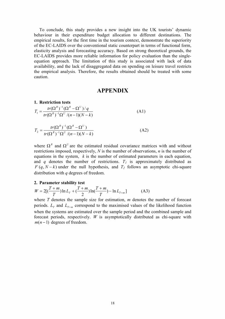
To conclude, this study provides a new insight into the UK tourists’ dynamic

behaviour in their expenditure budget allocation to different destinations. The

empirical results, for the first time in the tourism context, demonstrate the superiority

of the EC-LAIDS over the conventional static counterpart in terms of functional form,

elasticity analysis and forecasting accuracy. Based on strong theoretical grounds, the

EC-LAIDS provides more reliable information for policy evaluation than the single-

equation approach. The limitation of this study is associated with lack of data

availability, and the lack of disaggregated data on spending on leisure travel restricts

the empirical analysis. Therefore, the results obtained should be treated with some

caution.

APPENDIX

1. Restriction tests

))(1/()(

/)()(1

1

1kNntr

qtrT

UR

URR

−−ΩΩ

Ω−ΩΩ=

−

−

(A1)

))(1/()(

)()(1

1

2kNntr

trT

UR

URR

−−ΩΩ

Ω−ΩΩ=

−

−

(A2)

where RΩ and UΩ are the estimated residual covariance matrices with and without

restrictions imposed, respectively, N is the number of observations, n is the number of

equations in the system, k is the number of estimated parameters in each equation,

and q denotes the number of restrictions. T1 is approximately distributed as

) ,( kNqF − under the null hypothesis, and T2 follows an asymptotic chi-square

distribution with q degrees of freedom.

2. Parameter stability test

]ln)ln()2

(ln)[(2 mTT LT

mTmTL

T

mTW +−

+++

+= (A3)

where T denotes the sample size for estimation, m denotes the number of forecast

periods. TL and mTL + correspond to the maximised values of the likelihood function

when the systems are estimated over the sample period and the combined sample and

forecast periods, respectively. W is asymptotically distributed as chi-square with

)1( −nm degrees of freedom.

19

REFERENCES Anderson, G. and G. Mizon (1983). “Parameter Constancy Tests: Old and New.”

Southampton University Discussion Paper, no. 8325.

Attfield, C.L.F. (1997). “Estimating A Cointegrating Demand System,” European Economic

Review, 41: 61-73.

Balcombe, K. G. and J. R. Davis (1996). “An Application of Cointegration Theory in the

Estimation of the Almost Ideal Demand System for Food Consumption in Bulgaria.”

Agricultural Economics, 15: 47-60.

Bera, A. K., R. P. Byron and C. M. Jarque (1981). “Further Evidence on Asymptotic Tests for

Homogeneity and Symmetry in Large Demand Systems.” Economics Letters, 8: 101-

105.

Blanciforti, L., R. Green and G. King (1986). U.S. Consumer Behaviour over the Post-war

Period: An Almost Ideal Demand System Analysis. Monograph 40 (Giannini

Foundation of Agricultural Economics, University of California).

Chambers, M. J. (1993). “Consumers’ Demand in the Long Run: Some Evidence from UK

Data.” Applied Economics, 25: 727-733.

Chambers, M. J. and K. B. Nowman (1997). “Forecasting with the Almost Ideal Demand

System: Evidence from Some Alternative Dynamic Specifications.” Applied

Economics, 29: 935-943.

Court, R. H. (1968). “An Application of Demand Theory to Projecting New Zealand Retail

Consumption.” The Economic Review, 3: 401-411.

De Mello, M., A. Pack and M. T. Sinclair (2002). “A System of Equations Model of UK

Tourism Demand in Neighbouring Countries.” Applied Economics, 34: 509-521.

Deaton, A. and J. Muellbauer (1980). “An Almost Ideal Demand System.” American

Economic Review, 70: 312-326.

Deaton, A. (1974). “The Analysis of Consumer Demand in the United Kingdom, 1900-1970.”

Econometrica, 42: 341-361.

Dickey, D. A. and W. A. Fuller (1981). “Likelihood Ratio Statistics for Autoregressive Time

Series with Unit Roots.” Journal of the American Statistical Association, 79: 427-431.

Divisekera, S. (2003). “A Model of Demand for International Tourism.” Annals of Tourism

Research, 30: 31-49.

Duffy, M. (2002). “Advertising and Food, Drink and Tobacco Consumption in the United

Kingdom: A Dynamic Demand System.” Agricultural Economics, 1637: 1-20.

Durbarry, R. and M. T. Sinclair (2003). “Market Shares Analysis: The Case of French

Tourism Demand.” Annals of Tourism Research, 30: 927-941.

Eadington, W. R. and M. Redman (1991). “Economics and Tourism.” Annals of Tourism

Research, 18: 41-56.

Edgerton, D. L., B. Assarsson, A. Hummelmose, I. P. Laurila, K. Rickertsen and P. H. Vale

(1996). The Econometrics of Demand Systems with Applications to Food Demand in

the Nordic Countries. London: Kluwer Academic Publishers.

Engle, R. F. and C. W. J. Granger (1987). “Cointegration and Error Correction:

Representation, Estimation and Testing.” Econometrica, 55: 251-276.

Fujii, E., M. Khaled and J. Mark (1985). “An Almost Ideal Demand System for Visitor

Expenditures.” Journal of Transport Economics and Policy. 19: 161-171.

Granger, C. W. J. and P. Newbold (1974). “Spurious Regressions in Econometrics.” Journal

of Econometrics, 2: 111-120.

20

Johansen, S. (1988). “A Statistical Analysis of Cointegration Vectors.” Journal of Economic

Dynamics and Control, 12: 231-254.

Karagiannis, G. and K. Velentzas (1997). “Explaining Food Consumption Patterns in

Greece.” Journal of Agricultural Economics, 48: 83-92.

Karagiannis, G., S. Katranidis and K. Velentzas (2000). “An Error Correction Almost Ideal

Demand System for Meat in Greece.” Agricultural Economics, 22: 29-35.

Karagiannis, G. and G. J. Mergos (2002). “Estimating Theoretically Consistent Demand

Systems Using Cointegration Techniques with Application to Greek Food Data.”

Economics Letters, 74: 137-143.

Laitinen, K. (1978). “Why is Demand Homogeneity so often Rejected?” Economics Letters,

1: 187-191.

Leser, C. E. V. (1963). “Forms of Engel Functions.” Econometrica, 31: 694-703.

Lim, C. (1997). “An Econometric Classification and Review of International Tourism

Demand Models.” Tourism Economics,3: 69-81.

Lyssiotou, P. (2001). “Dynamic Analysis of British Demand for Tourism Abroad.” Empirical

Economics, 15: 421-436.

Meinser, J. F. (1979). “The Sad Fate of the Asymptotic Slutsky Test for Large Systems.”

Economics Letters, 2: 231-233.

O’Hagan, J. W. and M. J. Harrison (1984). “Market Shares of US Tourism Expenditure in

Europe: An Econometric Analysis.” Applied Economics, 16: 919-931.

Papatheodorou, A. (1999). “The Demand for International Tourism in the Mediterranean

Region.” Applied Economics, 31: 619-630.

Pashardes, P. (1993). “Bias in Estimation of the Almost Ideal Demand System with the Stone

Index Approximation.” Economic Journal, 103: 908-916.

Phillips, P. C. B. and P. Perron (1988). “Testing for A Unit Root in Time Series Regression.”

Biometrica, 75: 335-346.

Pyo, S., M. Uysal and R. McLellan (1991). “A Linear Expenditure Model for Tourism

Demand.” Annals of Tourism Research, 31: 619-630.

Ray, R. (1985). “Specification and Time Series Estimation of Dynamic Gorman Polar Form

Demand Systems.” European Economic Review, 27: 357-374.

Rickertsen, K. (1998). “The Demand for Food and Beverages in Norway.” Agricultural

Economics, 18: 89-100.

Song, H. and S. F. Witt (2000). Tourism Demand Modelling and Forecasting: Modern

Econometric Approaches. Oxford: Pergamon.

Stone, J. R. N. (1954). “Linear Expenditure Systems and Demand Analysis: An Application

to the Pattern of British Demand.” Economic Journal, 64: 511-527.

Syripopoulos, T. and T. Sinclair (1993). “A Dynamic Model of Demand for Mediterranean

Countries.” Applied Economics, 25: 1541-1552.

Syriopoulos, T. (1995). “A Dynamic Model of Demand for Mediterranean Tourism.”

International Review of Applied Economics, 9: 318-336.

White, K. (1985). “An International Travel Demand Model: US Travel to Western Europe.”

Annals of Tourism Research, 12: 529-545.

Witt, S. F. and C. A. Witt (1992). Modelling and Forecasting Demand in Tourism. London:

Academic Press.

Witt, S. F. (1995). “Forecasting Tourism Demand: A Review of Empirical Research.”

International Journal of Forecasting, 11: 447-475.

21

Working, H. (1943). “Statistical Laws of Family Expenditure.” Journal of the American

Statistical Association, 38: 43-56.

Zellner, A. (1962). “An Efficient Method of Estimating Seemingly Unrelated Regressions

and Test for Aggregation Bias.” Journal of the American Statistical Association, 57:

348-368.