modelling economic interdependencies of international ...epubs.surrey.ac.uk/810483/3/modelling...
TRANSCRIPT

Modelling Economic Interdependencies of
International Tourism Demand:
The Global Vector Autoregressive Approach
by
Zheng Cao
Submitted for the degree of
Doctor of Philosophy
School of Hospitality and Tourism Management
Faculty of Arts and Social Sciences
University of Surrey
April 2016
© Zheng Cao 2016

I
Declaration of Originality
This thesis and the work to which it refers are the results of my own efforts. Any
ideas, data, images or text resulting from the work of others (whether published or
unpublished) are fully identified as such within the work and attributed to their
originator in the text, bibliography or in footnotes. This thesis has not been submitted
in whole or in part for any other academic degree or professional qualification. I agree
that the University has the right to submit my work to the plagiarism detection service
TurnitinUK for originality checks. Whether or not drafts have been so-assessed, the
University reserves the right to require an electronic version of the final document (as
submitted) for assessment as above.
Signature:
Date: 22/12/2015

II
Abstract
Tourism demand is one of the major areas of tourism economics research. The current
research studies the interdependencies of international tourism demand across 24
major countries around the world. To this end, it proposes to develop a tourism
demand model using an innovative approach, called the global vector autoregressive
(GVAR) model.
While existing tourism demand models are successful in measuring the causal effects
of economic variables on tourism demand for a single origin-destination pair, they
tend to miss the spillover effects onto other countries. In the era of globalisation,
tourism destinations become interdependent on each other. Impacts of a distant event
can be transmitted across borders and be felt globally. Hence, modelling international
tourism demand requires one to go beyond a particular origin-destination pair, and
take into account the interdependencies across multiple countries. The proposed
approach overcomes the ‘curse of dimensionality’ when modelling a large set of
endogenous variables.
The empirical results show that, to different extents, co-movements of international
tourism demand and of macroeconomic variables are observed across all the 24
countries. In the event of a negative shock to China’s real income level and that to
China’s own price level, it is found that in the short run, almost all countries will face
fluctuations in their international tourism demand and their own price. But in the long
run the shocks will impact on developing countries and China’s neighbouring
countries more deeply than on developed countries in the West.
The current research contributes to the knowledge on tourism demand. It models
tourism demand in the setting of globalisation and quantifies the interdependencies
across major countries. On the practical front, tourism policy makers and business
practitioners can make use of the model and the results to gauge the scale of impacts
of unexpected events on the international tourism demand of their native markets.

III
Acknowledgement
Finishing the thesis is like seeing the light at the end of the tunnel. PhD is never an
easy journey. I sincerely thank every one who has offered help and care to me over
the years of my PhD study.
My sincerest gratitude goes to my supervisors, Prof Gang Li and Prof John Tribe, for
their invaluable advice and kind help throughout my research. I owe an enormous
debt of gratitude to Prof Gang Li for his extra support in my life, without which I
would not be able to settle into the new environment quickly and conduct my research
smoothly.
My thanks go to the School of Hospitality and Tourism Management, especially to
Prof Graham Miller, for the continuous and generous financial support. I appreciate
the assistance I have had from both the academic and the administrative staff within
the Faculty of Arts and Social Sciences. I am also grateful to my friends and fellow
researchers for their friendship and care.
Besides, I would like to extend my profound gratitude to Prof Haiyan Song in the
Hong Kong Polytechnic University, who has stimulated my interests in tourism
research and has been inspiring me since the very start of my academic career.
Last, but by no means the least, my deepest gratitude goes to my parents. They have
given me the unconditional support and love in my life. I dedicate this thesis to them.
Zheng Cao
22nd December 2015
Guildford, UK

IV
Table of Contents
DECLARATION OF ORIGINALITY ................................................................................................. I
ABSTRACT ........................................................................................................................................... II
ACKNOWLEDGEMENT .................................................................................................................. III
LIST OF TABLES .............................................................................................................................. VII
LIST OF FIGURES ............................................................................................................................. IX
LIST OF ABBREVIATIONS ............................................................................................................. XI
CHAPTER 1. INTRODUCTION ................................................................................................... 1
1.1 TOURISM IN A GLOBAL ENVIRONMENT.................................................................................... 1
1.2 CHALLENGES FOR TOURISM ECONOMICS RESEARCH ............................................................... 4
1.3 RESEARCH AIMS AND OBJECTIVES .......................................................................................... 5
1.4 STRUCTURE OF THIS RESEARCH .............................................................................................. 6
CHAPTER 2. TOURISM DEMAND AND ITS INFLUENCING FACTORS ........................... 8
2.1 INTRODUCTION ........................................................................................................................ 8
2.2 CONCEPTS AND DEFINITIONS ................................................................................................... 8
2.3 MEASUREMENT OF TOURISM DEMAND .................................................................................. 12
2.3.1 Tourism Expenditure ........................................................................................................ 15
2.3.2 Tourist Arrivals................................................................................................................. 16
2.3.3 Length of Stay ................................................................................................................... 17
2.4 INFLUENCING FACTORS OF TOURISM DEMAND...................................................................... 18
2.4.1 Economic Framework and Socio-Psychological Framework ........................................... 18
2.4.2 Microeconomic Foundations ............................................................................................ 24
2.4.3 Income .............................................................................................................................. 30
2.4.4 Prices ................................................................................................................................ 31
2.4.5 Travel Costs ...................................................................................................................... 34
2.4.6 Other Factors ................................................................................................................... 35
2.5 CONCLUSION ......................................................................................................................... 38
CHAPTER 3. TOURISM DEMAND MODELLING ................................................................. 39
3.1 INTRODUCTION ...................................................................................................................... 39
3.2 ECONOMETRIC MODELS ........................................................................................................ 39
3.2.1 The Single-Equation Approach ......................................................................................... 40
3.2.2 The System-of-Equations Approach .................................................................................. 53
3.2.3 Other Econometric Model ................................................................................................ 79
3.3 TIME SERIES MODELS ............................................................................................................ 81
3.3.1 Autoregressive Integrated Moving Average (ARIMA) Models ......................................... 82
3.3.2 Generalised Autoregressive Conditional Heteroskedasticity (GARCH) Models .............. 83
V
3.3.3 Other Time Series Models ................................................................................................ 85
3.3.4 Time Series Models Augmented With Explanatory Variables .......................................... 88
3.4 OTHER QUANTITATIVE METHODS ......................................................................................... 90
3.5 CONCLUSION ......................................................................................................................... 93
CHAPTER 4. INTERDEPENDENCIES OF TOURISM DEMAND ........................................ 94
4.1 INTRODUCTION ...................................................................................................................... 94
4.2 UNDERSTANDING GLOBALISATION ........................................................................................ 94
4.2.1 Globalisation, Globalism and Interdependence ............................................................... 94
4.2.2 The Globalisation Debate: Three Theses ......................................................................... 97
4.2.3 Spatio-Temporal Dimensions of Globalisation ................................................................ 99
4.3 ECONOMIC GLOBALISATION ................................................................................................ 103
4.3.1 The Driving Forces ......................................................................................................... 104
4.3.2 Manifestation of Economic Globalisation ...................................................................... 108
4.4 GLOBALISATION AND THE TOURISM SECTOR ....................................................................... 111
4.5 ECONOMIC INTERDEPENDENCIES OF INTERNATIONAL TOURISM DEMAND .......................... 115
4.5.1 Impacts of Inbound Tourism ........................................................................................... 116
4.5.2 Spillovers via Outbound Tourism ................................................................................... 121
4.5.3 Complementary and Substitutive Relations between Tourism Demand .......................... 124
4.6 EMPIRICAL AND THEORETICAL IMPLICATIONS .................................................................... 127
4.6.1 Business Cycle Synchronisation ..................................................................................... 127
4.6.2 China as an Emerging Economy .................................................................................... 136
4.6.3 Endogeneity Issue in Tourism Demand Modelling ......................................................... 137
4.7 CONCLUSION ....................................................................................................................... 140
CHAPTER 5. RESEARCH METHOD ...................................................................................... 141
5.1 INTRODUCTION .................................................................................................................... 141
5.2 THE GLOBAL VECTOR AUTOREGRESSIVE (GVAR) APPROACH ........................................... 141
5.2.1 Model Inference .............................................................................................................. 142
5.2.2 Model Specification ........................................................................................................ 146
5.2.3 Impulse Response Analysis ............................................................................................. 154
5.3 DATA DESCRIPTIONS ........................................................................................................... 157
5.3.1 Data Sources................................................................................................................... 157
5.3.2 Data Processing ............................................................................................................. 163
5.3.3 Setup of GVAR ................................................................................................................ 166
5.4 CONCLUSION ....................................................................................................................... 168
CHAPTER 6. EMPIRICAL RESULTS AND ANALYSIS ...................................................... 169
6.1 INTRODUCTION .................................................................................................................... 169
6.2 DESCRIPTIVE STATISTICS ..................................................................................................... 169
6.2.1 Basic Statistics ................................................................................................................ 169
VI
6.2.2 Unit Root Tests ............................................................................................................... 195
6.3 MODEL ESTIMATION RESULTS ............................................................................................. 195
6.3.1 Model Specification Parameters ..................................................................................... 198
6.3.2 Contemporaneous Impact Elasticities ............................................................................ 198
6.3.3 Persistence Profiles ........................................................................................................ 203
6.3.4 Diagnostic Tests ............................................................................................................. 210
6.4 IMPULSE RESPONSES............................................................................................................ 211
6.4.1 One Negative Shock to China’s Real Income ................................................................. 212
6.4.2 One Negative Shock to China’s Own Price .................................................................... 216
6.5 FURTHER DISCUSSIONS ........................................................................................................ 220
6.6 PRACTICAL IMPLICATIONS ................................................................................................... 223
6.6.1 Use of the Results ........................................................................................................... 223
6.6.2 Implications for the Major Countries ............................................................................. 225
6.7 CONCLUSION ....................................................................................................................... 228
CHAPTER 7. CONCLUSIONS .................................................................................................. 229
7.1 INTRODUCTION .................................................................................................................... 229
7.2 SUMMARY OF THE FINDINGS ................................................................................................ 229
7.3 LIMITATIONS OF THE CURRENT RESEARCH.......................................................................... 230
7.4 RECOMMENDATIONS FOR FUTURE RESEARCH ..................................................................... 232
APPENDICES .................................................................................................................................... 234
BIBLIOGRAPHY .............................................................................................................................. 275

VII
List of Tables
Table 1.1 - Tourism in the World: Key Figures in 2014 ........................................................... 1
Table 1.2 - Top destinations in terms of international tourist arrivals ....................................... 2
Table 1.3 - Top destinations in terms of international tourism receipts .................................... 2
Table 1.4 - Top spenders in terms of international tourism expenditure ................................... 3
Table 2.1 - Summary of Trade in Travel Services, UK ........................................................... 11
Table 2.2 - Tourism demand measures identified in previous review studies ......................... 13
Table 3.1 - Variations of the autoregressive distributed lag model ......................................... 45
Table 4.1 - Definitions of globalisation ................................................................................... 95
Table 4.2 - Top source countries for China’s inbound tourism ............................................. 133
Table 4.3 - Top destination countries for China’s outbound tourism .................................... 133
Table 5.1 - Summary of variables ......................................................................................... 147
Table 5.2 - Geographic coverage ........................................................................................... 159
Table 5.3 - Summary of data sources .................................................................................... 160
Table 5.4 - International tourist arrivals of selected countries .............................................. 161
Table 5.5 - International tourism receipts of selected countries ............................................ 162
Table 5.6 - Country level bilateral trade ................................................................................ 165
Table 5.7 - Country level trade shares ................................................................................... 165
Table 5.8 - Setting of model in GVAR Toolbox 2.0 ............................................................. 167
Table 6.1 - Correlations of nominal tourism imports between major countries .................... 179
Table 6.2 - Correlations of nominal tourism exports between major countries .................... 181
Table 6.3 - Descriptive statistics of country-specific domestic variables ............................. 183
Table 6.4 - Descriptive statistics of country-specific foreign variables ................................ 187
Table 6.5 - Descriptive statistics of global common variable ............................................... 191
Table 6.6 - Order of integration of each variable .................................................................. 193
Table 6.7 - Lag orders of country-specific VECMX models ................................................ 196
Table 6.8 - Number of cointegrations of country-specific VECMX models ........................ 197

VIII
Table 6.9 - Contemporaneous effects of foreign variables on domestic variables ................ 202
Table 6.10 - F-statistics for the serial correlation test of the VECMX residuals ................... 206
Table 6.11 - Test for weak exogeneity at the 5% significance level ..................................... 207
Table 6.12 - Average pairwise cross-section correlations: variables and residuals............... 208
Table 6.13 - Brief summary of the findings .......................................................................... 216
Table 6.14 - Brief summary of the findings .......................................................................... 220
Table A1 - Cointegrating vectors of the country-specific VECMX models ......................... 234
Table A2 - Estimates of individual VECMX models ............................................................ 239

IX
List of Figures
Figure 2.1 - Comparison between concepts ............................................................................ 14
Figure 2.2 - The economic and the socio-psychological framework ....................................... 21
Figure 2.3 - Trade-off between paid work and unpaid time .................................................... 27
Figure 2.4 - Consumption of toursim and other products ........................................................ 28
Figure 4.1 - Four potential forms of globalisation................................................................. 102
Figure 4.2 - Impacts on local economy by inbound tourism ................................................. 118
Figure 4.3 - Spillover effects of outbound tourism demand .................................................. 121
Figure 4.4 - Correlation between outbound demand and inbound demand ........................... 124
Figure 4.5 - China’s GDP growth rates ................................................................................. 134
Figure 4.6 - Trends of China’s inflation and exchange rate .................................................. 135
Figure 6.1 - Nominal tourism imports of selected countries (Million US$) ......................... 171
Figure 6.2 - Nominal tourism imports of selected Countries (Million US$) ......................... 172
Figure 6.3 - Nominal tourism imports of selected countries (Million US$) ......................... 173
Figure 6.4 - Nominal tourism imports of selected countries (Million US$) ......................... 174
Figure 6.5 - Nominal tourism exports of selected countries (Million US$) .......................... 175
Figure 6.6 - Nominal tourism exports of selected countries (Million US$) .......................... 176
Figure 6.7 - Nominal tourism exports of selected countries (Million US$) .......................... 177
Figure 6.8 - Nominal tourism exports of selected countries (Million US$) .......................... 178
Figure 6.9 - Persistence profile of the effect of system-wide shocks to the cointegrating
relations ................................................................................................................................. 205
Figure A1 - Generalised impulse responses of a negative shock to China’s real income on real
income across countries/regions ............................................................................................ 251
Figure A2 - Generalised impulse responses of a negative shock to China’s real income on
own price across countries/regions ........................................................................................ 254

X
Figure A3 - Generalised impulse responses of a negative shock to China’s real income on real
tourism imports across countries/regions .............................................................................. 257
Figure A4 - Generalised impulse responses of a negative shock to China’s real income on real
tourism exports across countries/regions ............................................................................... 260
Figure A5 - Generalised impulse responses of a negative shock to China’s own price on real
income across countries/regions ............................................................................................ 263
Figure A6 - Generalised impulse responses of a negative shock to China’s own price on own
price across countries/regions................................................................................................ 266
Figure A7 - Generalised impulse responses of a negative shock to China’s own price on real
tourism imports across countries/regions .............................................................................. 269
Figure A8 - Generalised impulse responses of a negative shock to China’s own price on real
tourism exports across countries/regions ............................................................................... 272

XI
List of Abbreviations
ADF Augmented Dickey-Fuller
ADLM Autoregressive Distributed Lag Model
AGARCH Asymmetric Generalised Autoregressive Conditional Heteroskedasticity
AGO Accumulated Generation Operation
AI Artificial Intelligence
AIC Akaike Information Criterion
AIDS Almost Ideal Demand System
ANN Artificial Neural Network
APD Air Passenger Duty
AR Autoregressive
ARFIMA Fractional Autoregressive Integrated Moving Average
ARIMA Autoregressive Integrated Moving Average
ARIMAX Autoregressive Integrated Moving Average model with explanatory
variables
ARMA Autoregressive Moving Average
BPM Balance of Payments and International Investment Position Manual
BOP Balance of Payments
BRICS Brazil, Russia, India, China and South Africa
BSM Basic Structural Model
CCC Constant Conditional Correlation
CI Co-Integration
CLSDV Corrected Least Squares Dummy Variable
CPI Consumer Price Index
CRS Computerised Reservations Systems
DF Dickey-Fuller test
DGP Data Generating Process

XII
DMO Destination Marketing Organisation
EC Error Correction
ECM Error Correction Model
ECT Error Correction Term
EGARCH Exponential Generalised Autoregressive Conditional Heteroskedasticity
ES Exponential Smoothing
FE Fixed Effects
GA Genetic Algorithms
GARCH Generalised Autoregressive Conditional Heteroskedasticity
GATS General Agreement on Trade in Services
GATT General Agreement on Trade and Tariffs
GDP Gross Domestic Product
GIR Generalised Impulse Response
GMM Generalised Method of Moments
GNP Gross National Product
GVAR Global Vector Autoregressive
HKTB Hong Kong Tourism Board
H-O Heckshcer-Olin
IATA International Air Transport Association
ICP International Comparison Programme
ILO International Labour Organisation
IMF International Monetary Fund
IOM International Organisation of Migration
IPS Im, Pesaran, and Shin
IV Instrument Variable
JML Johansen Maximum Likelihood
KF Kalman Filter
KPSS Kwiatkowski, Phillips, Schmidt, and Shin

XIII
LAIDS Linear Almost Ideal Demand System
LCC Latent Cycle Component
LES Linear Expenditure System
LLC Levin, Lin, and Chu test
LR Long-Run
LSDV Least Squares Dummy Variable
MA Moving Average
MAE Mean Absolute Error
MAPE Mean Absolute Percentage Error
MGARCH Multivariate Generalised Autoregressive Conditional Heteroskedasticity
ML Maximum Likelihood
MLP Multi-Layer Perceptron
NIE Newly Industrialising Economies
NTB Non-Tariff Barriers
OECD Organisation for Economic Co-operation and Development
OIR Orthogonalised Impulse Response
OLI Ownership-Location-Internationalisation
OLS Ordinary Least Square
ONS Office for National Statistics
PP Phillips-Perron
PPs Persistence Profiles
RBF Radial Basis Function
RMB Renminbi (Chinese currency)
RMSE Root Mean Square Error
ROW Rest of the World
SARIMA Seasonal Autoregressive Integrated Moving Average
SARS Severe Acute Respiratory Syndrome
SBC Schwarz Bayesian Criterion

XIV
SDR Special Drawing Right
SME Small and Medium-sized Enterprises
STSM Structural Time Series Model
SURE Seemingly Unrelated Regression Estimator
SVM Support Vector Machine
SVR Support Vector Regression
TGARCH Threshold Generalised Autoregressive Conditional Heteroskedasticity
TKIG Tourism exports-Capital goods imports-Growth
TLG Tourism-Led-Growth
TNC Transnational Corporations
TPI Toruist Price Indices
TSLS Two-Stage Least Squares
TVP Time-Varying-Parameter
TVP-LRM Time-Varying-Parameter Long-Run Model
UNWTO United Nations World Tourism Organisation
VAR Vector Autoregressive
VECM Vector Error Correction Model
VECMX Vector Error Correction Model with exogenous variables
VISTS Vector Innovations Structural Time-Series
VMA Vector Moving Average
WB Wickens-Breusch approach
WS-ADF Weighted Symmetric Augmented Dickey-Fuller
WTO World Trade Organisation
WTTC World Travel & Tourism Council
XCV Structural time series model with explanatory variables
3SLS Three-Stage Least Square

1
Chapter 1. Introduction
1.1 Tourism in a Global Environment
Internatioanl tourism is one of the most important sectors for an open economy. It is a
sector that is able to earn substantial foreign exchange, generate continuous
employment to local residents, and boost the national economy. That is why the
United Nations World Tourism Organisation (UNWTO) constantly describes tourism
as a ‘key to development, prosperity and well-being’ (UNWTO, 2013, 2014a, 2015).
Despite occasional shocks, tourism has shown almost uninterrupted growth over the
past few decades. International tourist arrivals have increased from 25 million
globally in 1950, to 278 million in 1980, 527 million in 1995, and 1,133 million in
2014. Correspondingly, international tourism receipts earned by destinations
worldwide have surged from US$ 2 billion in 1950 to US$ 104 billion in 1980,
US$ 415 billion in 1995 and US$ 1,245 billion in 2014 (UNWTO, 2015). Table 1.1
summarises some key figures of tourism in the world.
Table 1.1 - Tourism in the World: Key Figures in 2014
Economic output 9% of GDP - direct, indirect and induced impact
Employment 1 in 11 jobs
International Trade US$ 1.5 trillion in exports
6% of the world's exports
Movement of people from 25 million international tourists in 1950 to
1,133 million in 2014
1.8 billion international tourists forecast for 2030
Source: Adapted from UNWTO (2015)
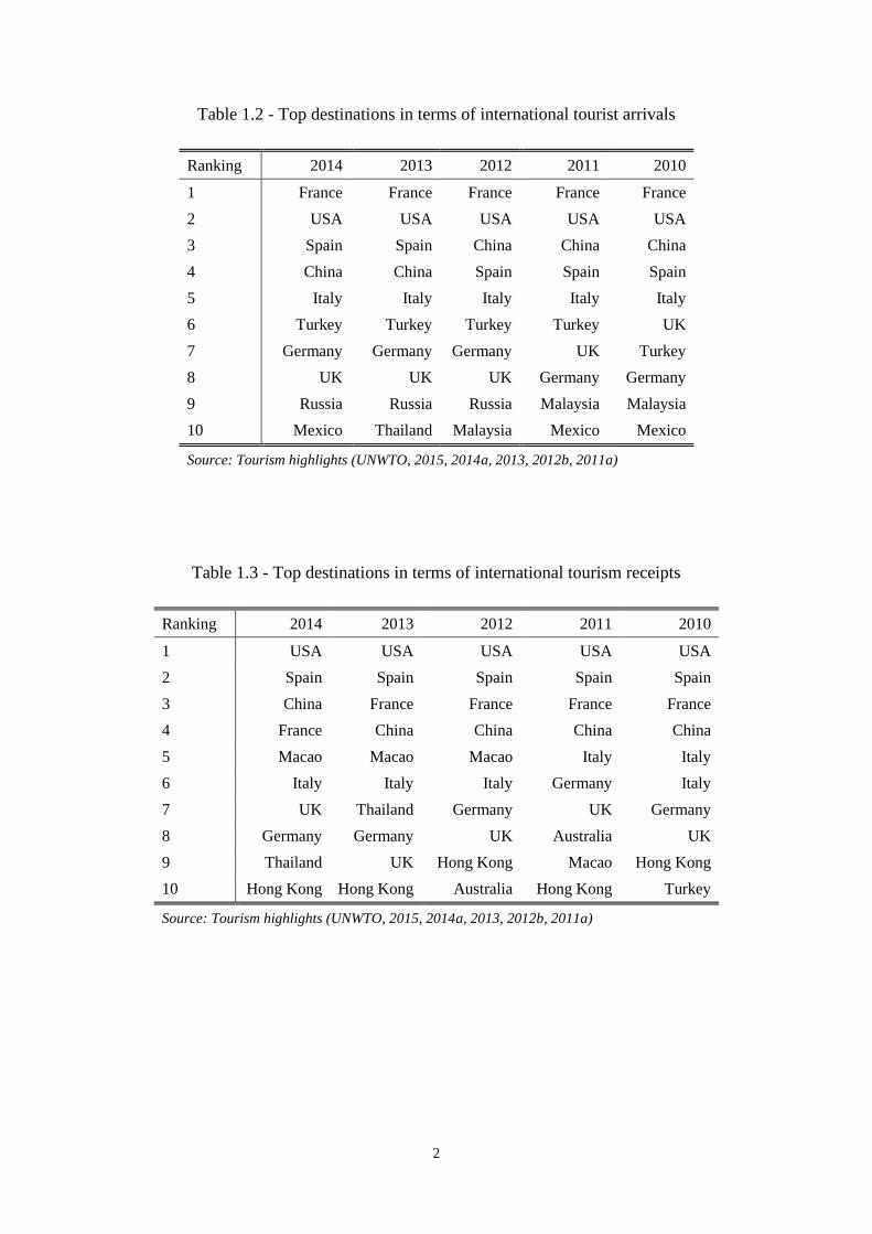
Major countries around the globe tend to actively engage in international tourism.
They are usually top destinations receiving thousands of millions of tourists every
year, while at the same time they are among the top spenders in overseas travel. Table
1.2, Table 1.3 and Table 1.4 show the major players in international tourism over the
recent five years.
2
Table 1.2 - Top destinations in terms of international tourist arrivals
Ranking 2014 2013 2012 2011 2010
1 France France France France France
2 USA USA USA USA USA
3 Spain Spain China China China
4 China China Spain Spain Spain
5 Italy Italy Italy Italy Italy
6 Turkey Turkey Turkey Turkey UK
7 Germany Germany Germany UK Turkey
8 UK UK UK Germany Germany
9 Russia Russia Russia Malaysia Malaysia
10 Mexico Thailand Malaysia Mexico Mexico
Source: Tourism highlights (UNWTO, 2015, 2014a, 2013, 2012b, 2011a)
Table 1.3 - Top destinations in terms of international tourism receipts
Ranking 2014 2013 2012 2011 2010
1 USA USA USA USA USA
2 Spain Spain Spain Spain Spain
3 China France France France France
4 France China China China China
5 Macao Macao Macao Italy Italy
6 Italy Italy Italy Germany Italy
7 UK Thailand Germany UK Germany
8 Germany Germany UK Australia UK
9 Thailand UK Hong Kong Macao Hong Kong
10 Hong Kong Hong Kong Australia Hong Kong Turkey
Source: Tourism highlights (UNWTO, 2015, 2014a, 2013, 2012b, 2011a)

3
Table 1.4 - Top spenders in terms of international tourism expenditure
Ranking 2014 2013 2012 2011 2010
1 China China China Germany Germany
2 USA USA Germany USA USA
3 Germany Germany USA China China
4 UK Russia UK UK UK
5 Russia UK Russia France France
6 France France France Canada Canada
7 Canada Canada Canada Russia Japan
8 Italy Australia Japan Italy Italy
9 Australia Italy Australia Japan Russia
10 Brazil Brazil Italy Australia Australia
Source: Tourism highlights (UNWTO, 2015, 2014a, 2013, 2012b, 2011a)
From the above tables, it is obvious that the major tourism origin and destination
countries are also major economies in the world. This is a suggestion of a close
relationship between international tourism and local economic development. It is also
observed that the top ten players in international tourism widely spread across
continents, even though many of them are in Europe. International tourism, as a part
of the world economy, involves an extensive area of countries.
As a sector that immensely engages with trade in goods and services, flows of foreign
exchange and movement of people, international tourism entails all the main aspects
of economic globalisation. It is through these three channels that the ties between
tourism destinations are strengthened. With growing interconnections, countries are
becoming more and more interdependent, especially economically.
As such, tourism businesses in a country are now operating in an increasingly global
environment. Not only are the incoming tourists strikingly diverse, but also the choice
of overseas destiantions for outgoing residents is becoming abundant. Moreover, more
and more businesses (for example, hotel groups and airlines) are extending their
geographical presence by forming multi-national corporations to reach out beyond
their native market. Consequently, tourism businesses are inevitably facing a broad
range of uncertainties at home and abroad. Uncertainties of macroeconomic

4
environment will ultimately reflect on the performance of local tourism businesses, in
terms of their revenues, costs, and profits.
On the one hand, tourism demand for a destination is greatly influenced by the
economic situation in the tourist-generating countries. The economic performance of
the destination is thus impacted on by the fluctuations in the origin countries. On the
other hand, as the residents of the destination travel to other overseas countries, they
further spillover the impacts. Hence, events in even a remote country can easily travel
across borders and cause global implications. Turmoils, or shocks, such as the
financial crisis in the USA, the great earthquakes in Japan and the political unrests in
the Arabic countries, are no longer confined to a single region. They exert influences
on other parts of the world as well.
Therefore, given the importance of tourism to economic development and the global
nature of business environment, it is of particular interests to tourism policy makers as
well as business practitioners to measure their interdependencies on other countries
and gauge the impacts of events on their tourism demand.
1.2 Challenges for Tourism Economics Research
Tourism demand is one of the most researched areas in tourism economics. Relevant
topics span from tourist behaviours at the micro level to tourist flows at the macro
level. Quantitative methods are widely used to model the destination choices of
tourists, to forecast the future levels of tourist flows and to assess the effects of
specific factors/events.
At the macro level, tourism demand analysis is particularly relevant to both policy
makers and business practitioners to monitor the trends of tourism demand. Tourism
businesses form their decisions of procurement, investment and employment based on
the expected values of future tourism demand and the expected effects of a change in
tourism demand determinants. Hence, tourism demand studies have extensive
practical significance.
Ever since the very early tourism demand studies in the 1960s, researchers have
developed and adopted various econometric models to account for the causal effects
of economic factors (in an origin country) on tourism demand (in a destination).
While the models are able to generate accurate forecasts, the results are usually
5
limited to a single origin-destination pair only. Aspects such as the effects on a
destination’s local economy and the spillovers to other destinations are thus not
modelled. From a theoretical point of view, this limitation arises because most of the
existing models only allow for a unidirectional causal relationship in one model.
Although attempts have been made to include multiple origin-destination pairs (hence
multiple causal relationships) in certain models, they tend to be hampered by the
relatively large number of parameters against limited observations of data.
As a result, within the existing tourism demand modelling frameworks, it is difficult
to properly quantify the interdependencies across countries in the world. In a
globalising setting, tourism destintions are increasingly reliant on each other
especially economically. Modelling tourist flows and gauging the impacts of a distant
event require one to go beyond a particular origin-destination pair, and take into
consideration the global interdependencies across countries.
Summing up the above points, a research gap is very clear that no existing studies
have modelled and analysed the economic interdependencies of tourism demand
across a number of countries on a global level. This can be further elaborated as
follows:
1. There are no tourism studies that discuss in great details why and how
international tourism sectors across different countries become interdependent
on each other, from the demand perspective;
2. There are no tourism studies that scientifically quantify the magnitude of
interdependencies across major countries in the world;
3. There are no tourism studies that simulate the impacts of a country-specific
shock on the major countries in the world.
The current research is set out to develop a tourism demand model using an
innovative modelling approach, which is able to overcome the limitations of existing
models.
1.3 Research Aims and Objectives
By filling the research gaps identified above, the current research aims to extend the
knowledge on international tourism demand. Specifically, the following questions are
to be answered:

6
1. To what extent will a country’s international tourism demand and its local
economy be affected by changes in its external world?
2. In the event of a shock to China, how much will the shock impact on other
countries’ international tourism demand and their local economies?
Answering the first question provides a measure of the degree to which a country is
integrated with the other parts of the world. The second question tests how deeply the
events in China can impact on other countries. Answers to the second question not
only indicates how closely the countries around the world are linked to each other, but
are also a reminder of the increasingly important roles played by emerging
economies.
To this end, an advanced modelling approach called global vector autoregressive
(GVAR) model is proposed to be used. The approach was developed by Pesaran,
Schuermann, and Weiner (2004) and further extended by Dee, Mauro, Pesaran, and
Smith (2007). It was initially applied to macroeconomic studies on global economic
linkages, and is appropriate for tourism demand studies in a global setting as well.
In view of the research gap and the research questions, the current research is
intended to achieve the following objetives:
1. To quantify the interdependencies of international tourism demand across
major countries;
2. To develop a tourism demand model using the GVAR approach;
3. To carry out simulations of China’s impacts on other countries’ international
tourism demand in the event of shocks to the Chinese economy;
4. To draw policy implications for major countries.
1.4 Structure of This Research
The current research is organised into seven full chapters, with the first being the
introduction and the last being the conclusions.
Chapter 2 to Chapter 4 are the literature reviews. Three main blocks of literature are
of particular relevance. Chapter 2 presents the basic concepts of tourism demand,
including the definitions and the measurement. Then much of the focus is placed on
the influencing factors of tourism demand, especially those that have been evidenced
by empirical models to play significant roles. In particular, the economic foundation

7
to reason the importance of those influencing factors is discussed in great details.
Chapter 3 then reviews the existing empirical models that feature in various tourism
demand studies. The chapter follows the usual divide of models into two major
groups. The first is econometric models, which account for the causal relationship
between economic factors and tourism demand. The other is time series models,
which only utilise information about the temporal characteristics of tourism demand
itself. In addition to the two major groups, an alternative group of models is briefly
introduced, which relies on artificial-intelligence (AI) techniques. Through
introducing the different groups of models, their limitations are reflected as well.
Chapter 4 focuses on the realistic background of the current research. Globalisation is
regarded as a backdrop that governs cross-country relationships in contemporary
times. As such, driving forces of globalisation and contesting scholarly views on the
development of globalisation are presented at length. However, much of the emphasis
is placed on the economic aspects and the interdependent nature of cross-country
relationship. That is because the specifications of econometric model in the current
research are informed in line with the reality of economic interdependencies across
countries. To resonate with one of the research objectives, some basic facts of the
Chinese economy will be presented. At the end of Chapter 4, the research gaps will be
further elaborated to justify the significance of the current research.
Chapter 5 and Chapter 6 are the empirical parts. Chapter 5 illustrates the modelling
process of GVAR approach and describes the data. Among the chapter’s sub-sections,
the model inference part is particularly important to understand the novelty of the
GVAR approach. Chapter 6 reports the main empirical results, discusses the findings
and draws the practical implications. The core results intended from the current
research are the contemporaneous impact elasticities and the impulse responses,
which answer the research questions.
In Chapter 7, the conclusions will be made with regard to the major findings,
contributions and limitations of the current research. The chapter, as well as the whole
research, will be concluded with some recommendations for future directions. It is
intended that, the current research will generate both theoretical and practical
contributions, and become a valuable addition to tourism economics literature.

8
Chapter 2. Tourism Demand and Its Influencing Factors
2.1 Introduction
Tourism demand has been one of the most researched areas in tourism economics. It
directly links to the economic performance of the tourism sector in a destination.
From a more practical point of view, modelling tourism demand constitutes a good
starting point for policy analysis and business strategy, as decisions are often formed
in an attempt to elicit or adjust to changes in tourism demand.
This chapter serves to understand the basic concepts of tourism demand, explore the
logic behind the formation of tourism demand and identify its influencing factors,
from both the theoretical and the empirical points of view. Section 2.2 highlights that
international tourism is first and foremost an integrated part of international trade. The
definition of tourism demand is thus delineated and contrasted based on the
terminology used by international organisations such as the International Monetary
Fund (IMF) and the United Nations World Tourism Organisation (UNWTO). Then
Section 2.3 proceeds to discuss the measurements of tourism demand, with a view to
revealing the implications behind each measure. Section 2.4 concerns tourists’
decision-making process and identifies the influencing factors. Specifically, consumer
demand theory is used to reason how consumers reach their travel decisions and what
factors they consider. Two broad sets of factors, i.e., economic and socio-
psychological, will be discussed accordingly. However, emphasis and elaboration will
be placed on the economic factors. After all, the goal here is not to provide an
exhaustive identification of the influencing factors, as this will tend to be
inconclusive. Instead, the link to economic theory is stressed. Given their high
relevance to the current research and certain pragmatic considerations in constructing
statistical models, the economic factors that have been suggested by theory and that
have recurrently been supported by empirical evidence will receive the major
attention.
2.2 Concepts and Definitions
The notion of tourism is associated with the activities of visitors. A visitor is someone
who takes a trip to a main destination outside his/her usual environment, for less than
a year, and for any main purpose (business, leisure or other personal purpose) other
than to be employed by a resident entity in the place visited (United Nations, 2010a,

9
p.10). These trips taken by visitors qualify as tourism trips. Synonymously, the IMF
uses the term travel to refer to tourism activities1 (IMF, 2005, p.64). Since the
literature from both the UNWTO and the IMF will be surveyed, the terms travel and
tourism will be referred to interchangeably henceforth.
An international visitor is a traveller who is a non-resident travelling in the country of
reference or a resident travelling outside of it on a tourism trip (United Nations,
2010a, p.16). Based on their length of stay, international visitors are disaggregated
into two categories, i.e., tourists (or overnight visitors) and same-day visitors (or
excursionists). Such a classification, as noted by United Nations (2010b), is helpful to
identify their significantly different structures of consumption.
As a major category of international trade, tourism activities are normally recorded
under the current account of the balance of payments (BOP), alongside other
components such as the trade in goods, financial services and other business services.
By nature, tourism is distinguishable from other trading activities in that it is a
demand-oriented activity. A visitor moves to the location of the provider
(organisations and residents of the economy visited) for the goods and services
desired by the visitor (IMF, 2005, p.64). In this sense, tourism is not a specific type of
service but an assortment of services consumed by visitors.
Broadly speaking, in relation to the country of reference, international tourism
consists of inbound tourism and outbound tourism. Inbound tourism corresponds to
the activities of a non-resident visitor within the country concerned on an incoming
tourism trip, whereas outbound tourism consists of the activities of a resident visitor
outside the country concerned either as part of an outward tourism trip or as part of a
domestic tourism trip (United Nations, 2010a, p.15). In the latter case, i.e., part of a
domestic trip, an example suggested by UNWTO (2014b, p.38) is that a person may
have to travel to a domestic city for his/her flight departure before travelling abroad.
While in that city he/she may stay there for a few days. This component of the whole
trip would be measured as a domestic visit.
1 It should be noted that conceptually there should be a distinction between travel and tourism. Travel
usually covers trips for any purpose and for any duration, which indicates tourism should be a subset of
travel. This is in accordance with UNWTO’s (United Nations, 2010a) recommendation. But in IMF’s
manual of balance of payments (IMF, 2005), a narrow definition of travel is adopted, and no such
distinction between travel and tourism is made.
10
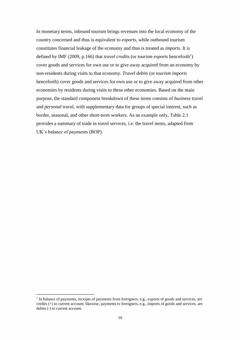
In monetary terms, inbound tourism brings revenues into the local economy of the
country concerned and thus is equivalent to exports, while outbound tourism
constitutes financial leakage of the economy and thus is treated as imports. It is
defined by IMF (2009, p.166) that travel credits (or tourism exports henceforth1)
cover goods and services for own use or to give away acquired from an economy by
non-residents during visits to that economy. Travel debits (or tourism imports
henceforth) cover goods and services for own use or to give away acquired from other
economies by residents during visits to these other economies. Based on the main
purpose, the standard component breakdown of these items consists of business travel
and personal travel, with supplementary data for groups of special interest, such as
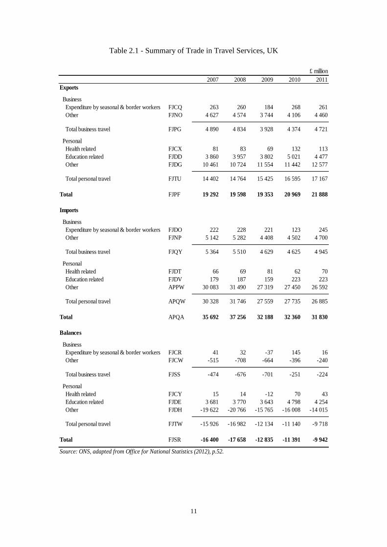
border, seasonal, and other short-term workers. As an example only, Table 2.1
provides a summary of trade in travel services, i.e. the travel items, adapted from
UK’s balance of payments (BOP).
1 In balance of payments, receipts of payments from foreigners, e.g., exports of goods and services, are
credits (+) to current account; likewise, payments to foreigners, e.g., imports of goods and services, are
debits (-) to current account.
11
Table 2.1 - Summary of Trade in Travel Services, UK
£ million
2007 2008 2009 2010 2011
Exports
Business
Expenditure by seasonal & border workers FJCQ 263 260 184 268 261
Other FJNO 4 627 4 574 3 744 4 106 4 460
Total business travel FJPG 4 890 4 834 3 928 4 374 4 721
Personal
Health related FJCX 81 83 69 132 113
Education related FJDD 3 860 3 957 3 802 5 021 4 477
Other FJDG 10 461 10 724 11 554 11 442 12 577
Total personal travel FJTU 14 402 14 764 15 425 16 595 17 167
Total FJPF 19 292 19 598 19 353 20 969 21 888
Imports
Business
Expenditure by seasonal & border workers FJDO 222 228 221 123 245
Other FJNP 5 142 5 282 4 408 4 502 4 700
Total business travel FJQY 5 364 5 510 4 629 4 625 4 945
Personal
Health related FJDT 66 69 81 62 70
Education related FJDV 179 187 159 223 223
Other APPW 30 083 31 490 27 319 27 450 26 592
Total personal travel APQW 30 328 31 746 27 559 27 735 26 885
Total APQA 35 692 37 256 32 188 32 360 31 830
Balances
Business
Expenditure by seasonal & border workers FJCR 41 32 -37 145 16
Other FJCW -515 -708 -664 -396 -240
Total business travel FJSS -474 -676 -701 -251 -224
Personal
Health related FJCY 15 14 -12 70 43
Education related FJDE 3 681 3 770 3 643 4 798 4 254
Other FJDH -19 622 -20 766 -15 765 -16 008 -14 015
Total personal travel FJTW -15 926 -16 982 -12 134 -11 140 -9 718
Total FJSR -16 400 -17 658 -12 835 -11 391 -9 942
Source: ONS, adapted from Office for National Statistics (2012), p.52.
12
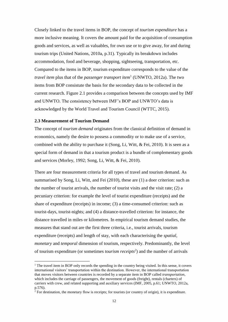
Closely linked to the travel items in BOP, the concept of tourism expenditure has a
more inclusive meaning. It covers the amount paid for the acquisition of consumption
goods and services, as well as valuables, for own use or to give away, for and during
tourism trips (United Nations, 2010a, p.31). Typically its breakdown includes
accommodation, food and beverage, shopping, sightseeing, transportation, etc.
Compared to the items in BOP, tourism expenditure corresponds to the value of the
travel item plus that of the passenger transport item1 (UNWTO, 2012a). The two
items from BOP consistute the basis for the secondary data to be collected in the
current research. Figure 2.1 provides a comparison between the concepts used by IMF
and UNWTO. The consistency between IMF’s BOP and UNWTO’s data is
acknowledged by the World Travel and Tourism Council (WTTC, 2015).
2.3 Measurement of Tourism Demand
The concept of tourism demand originates from the classical definition of demand in
economics, namely the desire to possess a commodity or to make use of a service,
combined with the ability to purchase it (Song, Li, Witt, & Fei, 2010). It is seen as a
special form of demand in that a tourism product is a bundle of complementary goods
and services (Morley, 1992; Song, Li, Witt, & Fei, 2010).
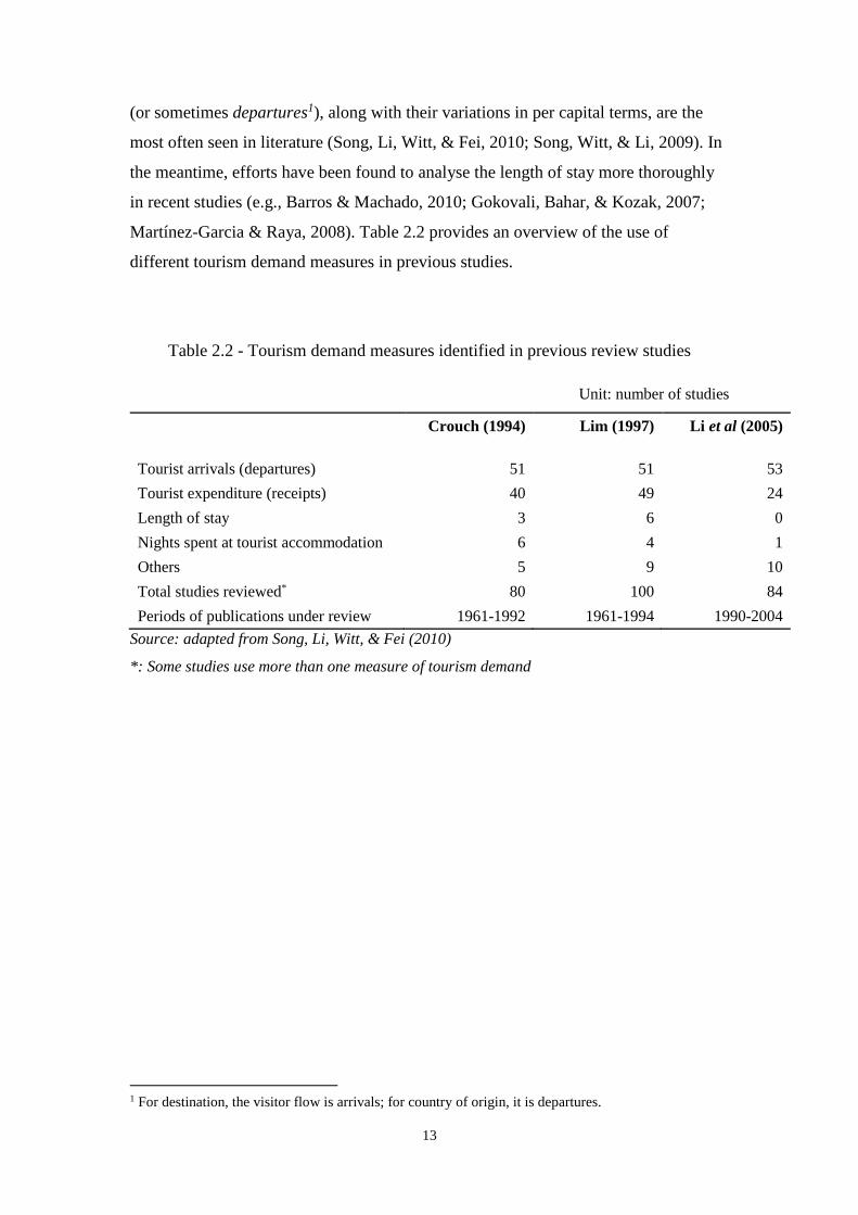
There are four measurement criteria for all types of travel and tourism demand. As
summarised by Song, Li, Witt, and Fei (2010), these are (1) a doer criterion: such as
the number of tourist arrivals, the number of tourist visits and the visit rate; (2) a
pecuniary criterion: for example the level of tourist expenditure (receipts) and the
share of expenditure (receipts) in income; (3) a time-consumed criterion: such as
tourist-days, tourist-nights; and (4) a distance-travelled criterion: for instance, the
distance travelled in miles or kilometres. In empirical tourism demand studies, the
measures that stand out are the first three criteria, i.e., tourist arrivals, tourism
expenditure (receipts) and length of stay, with each characterising the spatial,
monetary and temporal dimension of tourism, respectively. Predominantly, the level
of tourism expenditure (or sometimes tourism receipts2) and the number of arrivals
1 The travel item in BOP only records the spending in the country being visited. In this sense, it covers
international visitors’ transportation within the destination. However, the international transportation
that moves visitors between countries is recorded by a separate item in BOP called transportation,
which includes the carriage of passengers, the movement of goods (freight), rentals (charters) of
carriers with crew, and related supporting and auxiliary services (IMF, 2005, p.61; UNWTO, 2012a,
p.576). 2 For destination, the monetary flow is receipts; for tourists (or country of origin), it is expenditure.
13
(or sometimes departures1), along with their variations in per capital terms, are the
most often seen in literature (Song, Li, Witt, & Fei, 2010; Song, Witt, & Li, 2009). In
the meantime, efforts have been found to analyse the length of stay more thoroughly
in recent studies (e.g., Barros & Machado, 2010; Gokovali, Bahar, & Kozak, 2007;
Martínez-Garcia & Raya, 2008). Table 2.2 provides an overview of the use of
different tourism demand measures in previous studies.
Table 2.2 - Tourism demand measures identified in previous review studies
Unit: number of studies
Crouch (1994) Lim (1997) Li et al (2005)
Tourist arrivals (departures) 51 51 53
Tourist expenditure (receipts) 40 49 24
Length of stay 3 6 0
Nights spent at tourist accommodation 6 4 1
Others 5 9 10
Total studies reviewed* 80 100 84
Periods of publications under review 1961-1992 1961-1994 1990-2004
Source: adapted from Song, Li, Witt, & Fei (2010)
*: Some studies use more than one measure of tourism demand
1 For destination, the visitor flow is arrivals; for country of origin, it is departures.

14
Figure 2.1 - Comparison between concepts
Source: Summariesd by the author
Tourism receiptsInbound tourism
Outbound tourism
Tourism exports
Tourism imports Tourism
expenditure
• Travel items• Passenger transport items
Internationaltourism
Balance of Payments (BOP), IMF UNWTO

15
2.3.1 Tourism Expenditure
As defined by the United Nations (2010a, p.31), tourism expenditure covers all the
consumption of goods and services, as well as valuables, for and during tourism trips
by visitors. The concept therefore includes potentially all individual items deemed as
consumption goods and services by National Accounts. The use of tourism
expenditure measure, as noted by Song, Witt and Li (2009, p.27), is often associated
with system demand models, such as the linear expenditure system (LES) and the
almost ideal demand system (AIDS). On the practical front, tourism expenditure is a
straightforward measure of a destination’s economic performance, which is highly
relevant to destination competitiveness assessments (Li, Song, Cao, & Wu, 2013).
The primary data on tourism expenditure are usually surveyed at the border. Tourism
expenditure is often disaggregated into a variety of product categories. For example,
the United Nations (2010b, p.51) recommends a breakdown that encompasses
accommodation, food and beverage, transport, travel agency services, cultural
services, and etc. Once the questionnaire is set up, border surveys could be carried out
on a periodic basis. However, as with many other surveys, the data collected
inevitably suffer from certain biases, such as recall bias and memory effects
(Frechtling, 2006). This poses a question mark on how accurate the data of tourism
expenditure can be. Examples of empirical studies that employ surveyed expenditure
data are Li, Song, Cao, and Wu (2013) and Wu, Li, and Song (2012), both of which
used the annual tourism expenditure data reported by the Hong Kong Tourism Board
(HKTB).
An alternative estimation method would probably be using central bank data, by
borrowing trade in services figures from the balance of payments (BOP). Gray (1966)
and Artus (1972) are among the earliest and the few which analyse travel exports and
imports. Continuous efforts can be found in the studies by Smeral (2004), Smeral and
Weber (2000), and Smeral and Witt (1996), where tourism demand was defined as
real tourism exports and/or real tourism imports at base year (1985) price in US
dollar terms. The current research follows the same practice of using trade figures of
tourism as raw data.
One merit of trade figures is their high relevance to policy making. The balance
between exports and imports is often a government’s policy target, given that it will

16
have implications on other key indicators such as exchange rates, consumer price
index (CPI) and interest rates. Indeed, seeing international tourism as a form of
service trade also puts the sector into a bigger perspective. The trade figures of
tourism from the BOP can be directly compared to other figures such as exports and
imports of goods, commodities, and other services. This comparison helps
macroeconomic policy makers to gauge the developments across different sectors and
each sector’s competitiveness in a global environment.
In spite of the rich implications, the use of tourism exports and tourism imports
statistics is not without problem. As discussed by Frechtling (2006) and Stabler,
Papatheodorou and Sinclair (2010, pp.49-50), the validity of central bank data in
measuring tourism demand depends on how accurately and properly the foreign
exchange transactions related to tourist consumptions are recorded. For example,
tourists may pre-pay for an all-inclusive package in the origin, therefore spending
recorded at the destination may not fully reflect the tourists’ actual expenditures. The
problem will be more apparent in the case of a monetary union, where the boundary
of a nation remains but the different denominations of currency are removed.
2.3.2 Tourist Arrivals
As shown in Table 2.2, the tourist arrivals measure enjoys slightly more popularity
than the tourism expenditure measure. International visitor arrivals are usually
recorded at the border controls. Visa requirements, which although may impede
international tourism, could facilitate the collection of accurate statistics (Stabler,
Papatheodorou, & Sinclair, 2010, p.49). Such a measure of international travel is
often complemented with surveys of visitors at the border (or in its vicinity),
especially in the cases where no visa restrictions exist or the border controls have
disappeared (for example, movements within the Schengen area in Europe). Where
surveys of visitors at the border cannot be implemented, these could instead be
conducted at places of accommodation, as recommended by the United Nations
(2010a, p.18). Researchers can extract citizenship details from the registration form
filled by tourists when checking in, and also the number of nights spent in the
accommodation. However the accuracy of this method is often challenged, due to the
17
exclusion of day-trippers1 and the existence of tourists staying with friends or
relatives and illegal (or unregistered) lodgings (Song, Witt, & Li, 2009, p.3; Stabler,
Papatheodorou, & Sinclair, 2010, p.49).
As opposed to tourism expenditure, the visitor arrivals measure usually enjoys more
immediate availability as well as higher frequency (such as quarterly and monthly).
But as pointed out by Song, Li, Witt and Fei (2010), when the economic impact of
tourism is of concern, the tourist arrivals statistics cannot meet policy makers’ needs.
2.3.3 Length of Stay
The temporal definition of tourism demand, as shown in Table 2.2, has long been
underrepresented in the literature. It is seen as an alternative measure of tourism
demand (Song, Witt, & Li, 2009, p.2). Of all the studies surveyed by different
researchers at different periods, those that use the length of stay or nights spent as a
measure of tourism demand account for only around 10%, whereas the rest 90% were
shared between tourist expenditure and tourist arrivals measures (see Table 2.2).
In fact, the number of nights spent in tourist accommodation can directly measure the
demand for the hospitality sector, and thus has huge business implications. But the
exclusion of stays with friends or relatives often undermines the completeness of the
tourist nights spent statistics. A more inclusive measure, the length of stay, which
reflects the number of nights in the destinations and visitor days, is an alternative. It is
proposed that the length of stay has a crucial role in deciding total tourist spending.
The longer a tourist stays in a destination, the more money he/she is likely to spend
there. However, according to Gokovali, Bahar and Kozak’s (2007) survey of
literature, such a relationship between the length of stay and the money spent has not
been well established by empirical evidence. Hence, whether the length of stay can be
a robust measure of tourism demand is still debatable.
Nevertheless, more and more attention has recently been paid to accounting for the
determinants of length of stay (e.g., Barros, Butler, & Correia, 2010; Gokovali, Bahar,
& Kozak, 2007; Martínez-Garcia & Raya, 2008). Quantitative models such as
duration models (or survival models) are designed to investigate the roles of tourists’
socio-demographic profiles, holiday characteristics as well as economic factors in
1 It is worth reiterating that, as introducted in Section 2.2, an international visitor is categorised as
either a tourist (or overnight visitor) or a same-day visitor (or excursionist).

18
determining tourists’ length of stay. A number of factors with positive and/or negative
effects have been identified from those models. It is expected that those studies will
help better understand tourists’ behaviour, and hence the temporal dimension of
tourism demand.
2.4 Influencing Factors of Tourism Demand
The influencing factors of tourism demand are, in the first instance, identified in
relation to tourists’ decision-making process. Without discussing this process, it is not
possible to form a solid ground to suggest what factors and how they encourage or
deter tourism participation. By and large, two sets of factors, i.e., economic and socio-
psychological, are considered by theories. It is because of their utmost relevance that
economic factors will become the main focus of the current research.
2.4.1 Economic Framework and Socio-Psychological Framework
Tourism demand has predominantly been analysed on the basis of conventional
economic theory (Goh, 2012). Specifically, the backbone is consumer demand theory,
which interprets consumers’ decision-making process as solving utility maximisation
problems. On the one hand, in deciding how much to consume, the consumer demand
theory assumes a consumer will face a budget constraint, which is determined by the
income/budget available to him/her, and the prices of alternative products. Hence, the
budget constraint is directly related to objective (economic) factors. On the other
hand, the consumer is also influenced by his/her own preferences and tastes, which
are represented by a set of parallel indifference curves, with each of them denoting a
specific level of utility for the consumer. Apparently, the shaping of indifference
curve(s) is influenced by personal level subjective (non-economic) factors such as
socio-psychological factors and by perceptions of external attributes related to
destinations. The utility maximisation is then derived by finding the point where
graphically an indifference curve is tangent to the budget constraint (which will be
discussed in details in Section 2.4.2), which means the consumer gains the maximal
level of utility within his/her attainable financial means. The tangent point hence
denotes the consumption decision for alternative products.
2.4.1.1 Economic Framework: the Omission of Non-Economic Factors
Although the consumer demand theory does not rule out the influences of consumer’s
preferences, it is observed that econometric analysis of tourism demand

19
predominantly focuses on objective factors only, such as income and consumer prices
(e.g., Artus, 1972; Lim, 1997; Li, Song, & Witt, 2005; Morley, 1998; Song, Witt, &
Li, 2009). Thereafter, the economic framework is narrowly defined as one that only
concerns economic factors and the associated budget constraints. On the one hand, the
narrower framework examines tourism demand principally at the aggregate level.
Even if the income and the consumption patterns are rather heterogeneous at the
individual level, it is observable that aggregate demand exhibits coherent responses
towards economic fluctuations. From a practical point of view, comparable cross-
country data are regularly available at the macroeconomic level. This convenience
undoubtedly enables in-depth analyses of tourism demand from an macroeconomic
perspective. On the other hand, a major reason for omitting the non-economic factors
is the lack of available data and the difficulty in obtaining exact measures for these
factors (Goh, 2012). Goh (2012, p.1863) further argues that, ‘perhaps the true reason
for the omission of more determining factors lies in the expense incurred in
developing increasingly complex models in exchange for their inclusion’. Indeed,
compared to human behaviour, statistical models are rather restrictive and sometimes
too simple. The accuracy of statistical estimation largely depends on the degrees of
freedom, which are proportional to the number of observations in the sample and
inversely related to the number of parameters to be estimated. To accommodate an
extensive range of factors, a statistical model will easily exhaust the degrees of
freedom, making the estimation problematic. Besides, all statistical models follow
certain assumptions, the breach of which will result in biases. For example, most
models require explanatory variables to be exogenous to the dependent variable and
no multicollinearity among the explanatory variables. In other words, there should not
be any feedback influences from the dependent variable to the explanatory variables,
and the explanatory variables themselves should not be interrelated. Such assumptions
can be too rigid when socio-psychological factors are considered, as they tend to be
interactive. Moreover, the influence of certain non-economic factors may have
already been well captured by the economic factors indirectly. For example, a nation’s
income level is associated with the age structure as well as the average education level
of the society. If income, age and education are included in one model, it is likely to
create multicollinearity problem and yield biased results.

20
2.4.1.2 Socio-Psychological Framework
Despite the difficulties in incorporating non-economic factors into tourism demand
models, efforts have been made to develop a socio-psychological framework that
deals with the shaping of a consumer’s preferences and tastes. It states that people
have unlimited wants and that these wants are turned into motives by certain stimuli,
which in turn become demand when backed by buying power (Goh, 2012).
Following Um and Crompton (1990), destination choice is influenced by internal
inputs and external inputs. Internal inputs are the socio-psychological set of a
traveller’s personal characteristics (socio-demographics, life-style, personality, and
situational factors), motives, values, and attitudes. For example, a classic idea by
Stanley Plog, as reviewed by Stabler, Papatheodorou, and Sinclair (2010, p.40), is that
tourists can be categorised on a spectrum ranging from ‘allocentric’ to
‘psychocentric’, with the former referring to those who are more adventurous and
self-confident whereas the latter referring to those who prefer familiar and reassuring
locations and social interactions. External inputs can be viewed as the sum of social
interactions and marketing communications to which a potential traveller is exposed.
Furthermore, the external inputs can be classified into significative stimuli (which
emanate from actually visiting the destination), symbolic stimuli (which are the words
and images in promotional material by the travel industry), and social stimuli (which
emanate from other people in face-to-face interactions) (Um & Crompton, 1990). An
important conceptual framework which is based on the destination attributes
(equivalent to the significative stimuli) is the Lancaster’s characteristics framework,
which was proposed by Lancaster (1966) and Gorman (1980). The idea is that
products themselves do not give utility to the consumer; they possess certain
characteristics; it is the consumption of these characteristics that gives utility (Goh,
2012; Stabler, Papatheodorou, & Sinclair, 2010, pp.36-39). In tourism research, the
characteristics that are often under consideration are generally related to destination
attractions (natural and built) and facilities (e.g., hotels, airports, and ancillary
services) (Stabler, Papatheodorou, & Sinclair, 2010, pp.36-39).

21
Figure 2.2 - The economic and the socio-psychological framework
Source: Adapted from Goh (2012) and Um and Crompton (1990)
External Inputs Internal Inputs
Economic Framework Socio-Psychological Framework
Budget Constraint Indifference Curve / Utility Function
• Incomes
• Price Level of Destination
• Price Level of Alternative Destinations
• Exchange Rates
Stimuli Display:
• Significative
• Symbolic
• Social
Socio-Psychological Set:
• PersonalCharacteristics
• Motives
• Values
• Attitudes
Consumer Demand
budget constraint tangent to indifference curve

22
2.4.1.3 Which Framework to Follow: Methodological Considerations
Admittedly, a comprehensive study of tourism demand should involve both the
economic and the socio-psychological aspects. Figure 2.2 summarises the building
blocks of the economic and socio-psychological frameworks, based on Goh (2012)
and Um and Crompton (1990). The economic framework is often criticised for
ignoring demographic differences (Morley, 1995) and for its limited success in
explaining human behaviour (Goh, 2012). In an ideal world, when studying tourism
demand, non-economic factors should take the same weightings as their economic
counterparts (Goh, 2012). In reviewing the theoretical studies of people’s motivation
for travelling, Stabler, Papatheodorou, and Sinclair (2010, p.40) comment, the studies
of motivation ‘seek to explain the reasons for behaviour which economists observe
only from preferences which are revealed in terms of expenditure on goods and
services in the market. In this respect, the study of motivation assists in making more
accurate explanations and forecasts of the level and pattern of tourism demand’.
However, such a combination of both frameworks has to be taken very cautiously. On
the one hand, while the economic framework allows for analysis at both the aggregate
and the individual level (as long as the relevant data are available at that level1), the
socio-psychological framework stimulates studies mainly from the perspective of
individuals (e.g., Crouch, Devinney, Louviere, & Islam, 2009; Lyons, Mayor, & Tol,
2009; Wu, Zhang, & Fujiwara, 2013). On the other hand, the economic factors
indicated by the economic framework are generally well justified by economic theory,
whereas the interpretation of non-economic factors tends to be less theory-based. For
example, in the log-log form of demand models, the coefficients on economic factors
(such as income and prices) can be easily interpreted as demand elasticities, while the
interpretation of the coefficients on non-economic factors is usually not that
straightforward. Hence, the inclusion of non-economic factors into an econometric
(causal) model tends to be challenged for lack of a firm theoretical underpinning.
From a more pragmatic perspective, the feasibility of constructing a robust stastistical
model has also to be taken into consideration. As discussed earlier on, the omission of
non-economic factors in some studies is often associated with statistical
1 This can usually be met, as specialised databases for micro- and/or macro-economic data are
generally accessible to academics.

23
considerations, such as the degrees of freedom, the exogeneity assumption and the
multicollinearity problem. To follow a combined framework, the potential statistical
issues have to be carefully considered beforehand. Simply gathering a large set of
socio-psychological factors does not guarantee valid and meaningful statistical results.
Perhaps the last but not the least consideration is the data structure. This can be briefly
described as an issue of temporal versus spatial. Economic data are generally
available in the form of time series, i.e., observations over a period of time, and also
in the form of cross-sectional series, e.g., cross countries/industries. This flexibility
allows economic data to be analysed by different types of models, such as time series
models and panel data regression models. On the contrary, socio-psychological data
are in general arranged cross-sectionally, because these factors are relatively time-
invariant or it would be difficult to obtain observations over a long time span. For
example, social surveys to measure non-economic factors (e.g., the disability rates of
the population, for accessible tourism) are not necessarily conducted continuously
over a long period of time, and no time series of non-economic factors are available.
Hence, it would be more realistic to apply only certain types of models to socio-
psychological data, such as simple regression and cross sectional data regression. In
other words, when the temporal dimension of variables (say, the fluctuations of
tourism demand over time) is of concern, it would be more appropriate to follow the
economic framework. In that case, leaving out socio-psychological factors will not
cause much loss of information, because these factors and their effects will remain
stable.
Admittedly, the data to be gathered and the model to be used should be dictated by the
theoretical framework, rather than the other way round. The discussions above only
intends to show that, successful modelling will involve certain statistical restrictions,
which in turn act as constraints onto the choice of theoretical framework.
The setting of the current research is a global environment, where from year to year
tourism markets face economic turbulences. Tourism itself, as a principal part of
international trading activities, intertwines with the globalisation process extensively.
As such, interdependencies between tourism demand across different destinations are
observable in the form of co-movements. Hence, to address the interdependent
relations of tourism demand, economic variables are in the pivotal position to explain

24
the linkages between destinations. Logically, the current research and the following
review will thus be largely based on the economic framework.
2.4.2 Microeconomic Foundations
Tourism demand is usually studied at the aggregate level (for example, the number of
tourist arrivals to a certain country). A tendancy in macroeconomics is to seek
microeconomic foundations, which facilitates better understanding of the mechanism
underpinning macroeconomic phenomena. Likewise, the economic analysis of
aggregate tourism demand also needs to be built on rigorous micro-groundings. As
Backhouse (2010, p.121) remarks,
“macroeconomic relationships are the outcome of decisions by millions of
individuals, which means that if the subject (macroeconomics) is to be rigorous, it
must be based on a theory of how individuals behave.”
To understand the determinants of tourist flows, it is crucial to take account of the
factors that a tourist needs to weigh up when he/she makes travel decisions. Having
said that, on the one hand, it does not imply all the idiosyncratic factors surrounding
individuals must appear in a tourism demand model. Indeed, only a small number of
the factors, which influence people universally, will be of concern. The search for
microeconomic foundations (or micro-foundations), in the context of tourism
research, is to tackle the logic behind the influences of those ‘universal’ factors on
tourism demand. On the other hand, it does not imply that the parameters estimated
from a tourism demand model perfectly match every individual’s behaviour. The
models can only be meaningful in the aggregate sense, depicting the behaviour of
people as a group rather than as individuals. This relationship between the aggregate
level and the individual level is referred to as aggregation bias.
2.4.2.1 The Multi-Stage Budgeting Process
Following the consumer demand theory, the demand for tourism is determined by
people’s preferences and their budget constraints. The microeconomic foundations of
tourism demand first and foremost concern an individual’s decision making process.

25
To arrive at his/her travel decision, a tourist is assumed to undergo a multi-stage
process. He/she firstly trades off paid time1 against unpaid time. Paid work results in
income for consumption, hence decides the budget that can be spent in unpaid time.
Then he/she compares the prices of tourism products and those of other
goods/services, and decides the optimal combination of tourism products and other
goods/services. Once the budget on tourism products is allocated, the next step for
him/her is to decide which destination(s) to go, by comparing the prices of a number
of alternative destinations. It stands out that this multi-stage process is largely
constrained by economic factors such as income and prices. Nevertheless it should not
be overlooked that the exact combination that the tourist ends up with (for example,
how much paid work to take, how many nights of holiday to go) is down to his/her
personal preferences.
To elaborate the multi-stage process, certain simplifying and restrictive assumptions
are made, which are the composite commodity theorem2 and the separability of
preferences (Candela & Figini, 2012, p.142; Smeral & Weber, 2000; Stabler,
Papatheodorou, & Sinclair, 2010, p.27). The composite commodity theorem states that
various products can be aggregated into broad bundles of products. Each bundle can
be treated as if it were a single product, provided that prices within the bundle move
in parallel (i.e., the relative prices of products within it remain unchanged). Indeed, it
is reasonable to assume that a consumer perceives a broad group of relevant products
as a unity, since it is unlikely for him/her to be fully aware of the difference of price
changes in each individual product. The other assumption, the separability of
preferences, states that preferences within one bundle are independent of those in
another. For example, a consumer’s choice of food can arguably be determined in
isolation from his/her consumption of clothes. In multi-stage budgeting, this implies
that the budget allocation at the former stage will not affect the latter. A total utility
can be achieved by summing up all the values of sub-utilities from each stage.
Though restrictive, both the composite commodity theorem and the separability of
preferences are devised to simplify the simulation of the real decision-making
process, so that only the most relevant elements of the process are dealt with.
1 This could result from paid work. Employees may be entitled paid holiday, which is associated with
their paid work. 2 It is called the aggregation theorem in some references (e.g., Candela & Figini, 2012, p.142)

26
With the above in mind, the multi-stage budgeting process can be elaborated using the
budget constraint and the indifference curve(s) as an analytical tool. The first stage is
about how much leisure time to take. Apparently, the more time for leisure, the less is
for work. The less time spent at work, the less income made available to the tourist,
which ultimately limits his/her affordability of leisure activities. Just as Stabler,
Papatheodorou and Sinclair (2010, p.24) comment,
“there is, however, a tension as income is often required to undertake leisure
pursuits (including tourism) so that the latter have an imputed ‘price’ or
opportunity cost.”
The situation is often associated with the so-called ‘leisure paradox’ (Cooper,
Fletcher, Gilbert, Fyal, & Wanhill, 2005, p.117), which depicts the negative
relationship between time and discretionary income in an individual’s life cycle.
Figure 2.3 illustrates the different combinations of consumption and unpaid time that
a tourist may have. Line CB is the budget constraint facing the individual, as it
represents all the maximal combinations that are affordable. Point C (perhaps a
workaholic) means all his/her time is devoted to work and thus he/she earns the
highest level of income, among all his/her options on line CB. Point B means all
his/her time is devoted to unpaid activities, thus there is no income from work but
only the unemployment benefits at level C*. Any other combinations of consumption
and unpaid time, such as point E and D, are financially feasible and ultimately depend
on the position of the individual’s indifference curve (e.g., I1, I2 for two different
individuals), which is entirely associated with his/her personal preferences. The
indifference curves are actually a set of parallel curves unique to each individual,
denoting different levels of utility for the individual. The farther away it is from point
O, the higher the utility is. Therefore, the intersection of the budget constraint line CB
and the indifference curve I1 (or I2) represents the optimal level of consumption
combination, because point E (or D) is the highest level of utility that Individual 1 (or
2) can achieve and still within his/her budget. In Figure 2.3, point E is achieved by
someone who values work highly, and point D by someone who enjoys free time
more in spite of lower consumption level attained.

27
Figure 2.3 - Trade-off between paid work and unpaid time
Source: Adapted from Stabler, Papatheodorou, & Sinclair (2010, p.25)
Here, the slope of line CB (i.e., how steep the line is) is apparently down to the wage
rate. With total time (line OU) being fixed (24 hours at maximum, and do not forget
one needs time for sleep), and the unemployment benefits being relatively stable (i.e.,
C* and B are fixed), the higher the wage rate, the higher point C will be, and hence the
steeper the line. Therefore, the wage rate, hence the disposable income, and the
possible unemployment benefits, are crucial factors in the tourist’s budgeting process.
The second stage is about the allocation of income (resulting from the previous stage)
to tourism and other goods/services. As illustrated in Figure 2.4, line TDG contains all
affordable combinations, with point T representing the maximum quantity of tourism
products to be consumed, and point G the maximum of other products. Here, all
products other than tourism are aggregated as if they were one product, which follows
the composite commodity theorem.
B
O U2 U1 U
C*
C1
C2
CE
I2
I2
D
I1
I1
Unpaid TimePaid Time
Con
sum
ptio
n,In
com
e
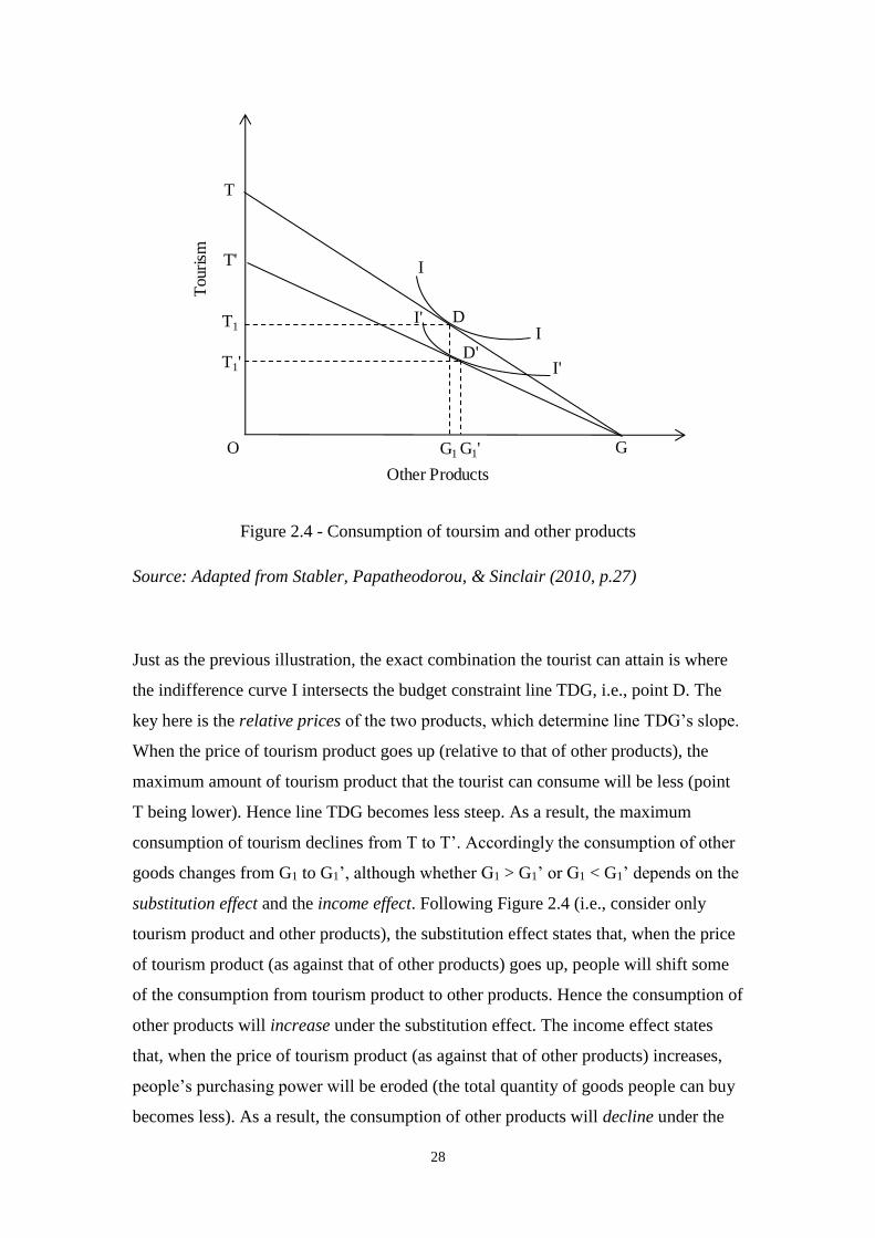
28
Figure 2.4 - Consumption of toursim and other products
Source: Adapted from Stabler, Papatheodorou, & Sinclair (2010, p.27)
Just as the previous illustration, the exact combination the tourist can attain is where
the indifference curve I intersects the budget constraint line TDG, i.e., point D. The
key here is the relative prices of the two products, which determine line TDG’s slope.
When the price of tourism product goes up (relative to that of other products), the
maximum amount of tourism product that the tourist can consume will be less (point
T being lower). Hence line TDG becomes less steep. As a result, the maximum
consumption of tourism declines from T to T’. Accordingly the consumption of other
goods changes from G1 to G1’, although whether G1 > G1’ or G1 < G1’ depends on the
substitution effect and the income effect. Following Figure 2.4 (i.e., consider only
tourism product and other products), the substitution effect states that, when the price
of tourism product (as against that of other products) goes up, people will shift some
of the consumption from tourism product to other products. Hence the consumption of
other products will increase under the substitution effect. The income effect states
that, when the price of tourism product (as against that of other products) increases,
people’s purchasing power will be eroded (the total quantity of goods people can buy
becomes less). As a result, the consumption of other products will decline under the
I'
I'D'
D
I
I
O G1 G
Other Products
T1
TT
ouri
sm
G1'
T1'
T'

29
income effect. In sum, as long as price change takes place on either of the two
products, both the substitution effect and the income effect will be present, although
the magnitude of either effect may vary from case to case.
The third stage of the multi-budgeting process is to choose the combination of tourism
products, such as different destinations, different types of tourism (cultural, adventure,
medical, etc.). The process is exactly the same as the illustration in Figure 2.4, with
the vertical and the horizontal axes respectively denoting different tourism products.
Again, the relative prices of destinations or tourism types play a pivotal role in
deciding the optimal combination of consumption. Based on the separability of
preferences, once the budget to be spent on tourism is allocated at the second stage,
the choice of a specific tourism product is an entirely independent decision,
irrespective of how much to be spent on other products. The budgeting process can
continue through subsequent stages with regard to the consumption of sub-products at
the destination, such as sightseeing, food and beverage, accommodation, and
transport.
2.4.2.2 The Aggregation Problem
Since the microeconomic foundations mainly concern the influencing factors at the
individual level, a link between the individual demand and the aggregate demand
needs to be addressed. This helps to justify why the factors recognised at the micro
level are appropriate for aggregate tourism demand models.
Traditionally in macroeconomics, the aggregation problem is understood using the
notion of ‘representative agent’, which is a typical decision-maker of a certain group
of identical agents. More broadly, the ‘representative agent’ concept is also deemed
appropriate even if the agents are heterogeneous, as long as they act in such a way
that the sum of their choices is mathematically equivalent to the decision of one
individual or many identical individuals. Though restrictive, the notion places
emphasis on the similarity of people’s decision-making. So ‘representative’ factors
are appropriate for aggregate models. Empirically, Blundell and Stoker (2005) survey
a number of econometric models that involve treatments of heterogeneity and
nonlinearlity at the individual level, in the areas of consumer demand analysis,
consumption growth and wealth, and labour participation and wages.

30
Mathematically, the aggregation problem can be addressed given certain assumptions.
Consider an economy with N consumers, each has a unique demand function
𝑞𝑖(𝑝, 𝑤𝑖), where p denotes a vector of prices for L goods and everyone faces the same
prices, 𝑤𝑖 is the income level of individual i (𝑤𝑖 can also denote the wealth level,
which is the accumulation of income over time). The relationship between aggregate
demand and individual demand follows:
𝑞(𝑝, 𝑤1,⋯ , 𝑤𝑁) = ∑ 𝑞𝑖(𝑝, 𝑤𝑖)𝑁𝑖=1 (1.1)
If individual i’s income, 𝑤𝑖, is generated by a process that is only related to prices (p)
and aggregate income (alternatively, aggregate wealth, denoted by w), then 𝑤𝑖 =
𝑤𝑖(𝑝, 𝑤). This can be justified by the fact that people’s income is mainly determined
by wage rate (or ‘price’ of leisure) and by taxes and/or government transfers (which
may entirely depend on aggregate income level). Then
∑ 𝒒𝒊(𝒑,𝒘𝒊)𝑵𝒊=𝟏 = ∑ 𝒒𝒊(𝒑,𝒘𝒊(𝒑,𝒘))
𝑵𝒊=𝟏 = ∑ 𝒒𝒊(𝒑,𝒘)
𝑵𝒊=𝟏 = 𝒒(𝒑,𝒘) (1.2)
Hence, if a certain distribution rule 𝑤𝑖 = 𝑤𝑖(𝑝, 𝑤) exists, it is appropriate to model
aggregate demand as a function of prices and aggregate income.
Morley (1995) discusses the aggregation problem in the context of tourism. He
proposes an alternative approach, which was based on a random utility model. The
central idea is to assume that the utilities are not fully determined but have a random
element, which results from errors in the individual’s perceived values of relevant
variables, the impact of variables other than those explicitly incorporated into the
utility function and/or the effect of random events. Assuming that the individual
demand is mutually independent and that the Central Limit Theorem applies, the
aggregate demand (i.e., the add-up of individual demand) is shown to be a function of
individual level factors. Hence, it justifies the applicability of variables at the micro
level for aggregate analysis.
2.4.3 Income
Based on the microeconomic foundations of tourism demand, it is not surprising that
income enters a tourism demand model as a key variable. Of the 100 studies reviewed
by Lim (1997), 84 studies employ income as one of the explanatory variables, topping
the list of all variables used. The measures (or proxies) of income can vary.

31
Disposable income, GDP and GNP, in nominal or real terms and in their per capita
form, can all be considered. As a rule of thumb, if holiday visits or visits to friends
and relatives are being studied, the appropriate form of variable is private
consumption or personal disposable income; if the focus is on business visits, a more
general income variable such as national income should be used (Witt & Witt, 1995).
It is acknowledged that tourism demand is not only influenced by the current income
level, but also by its lagged level (i.e., its past value), since it takes time for changes in
income to affect tourism demand (Lim, 1997). This brings up an issue whether
consumer behaviour is backward-looking or forward-looking. If tourists are
backward-looking (i.e., they care about how much they have earned), lagged values of
income would be relevant to their decision making; if they are forward-looking (i.e.,
they base their consumption decision on the expectation of future income), the present
value of their future income would affect their current demand (Stabler,
Papatheodorou, & Sinclair, 2010, p.52). In practice it is, however, more common that
lagged income variables are included, which is in line with the backward-looking
perspective. The forward-looking aspect of tourist behaviour is much less explored,
which could be due to the additional information required such as the prediction of
future income and the appropriate interest rate to discount future income.
2.4.4 Prices
Prices of products are crucial factors in forming tourists’ budget constraint, for any
changes in prices can result in rotation of the budget constraint and hence changes in
the optimal combination of consumptions (see Figure 2.4). In empirical studies, the
price variable should basically contain two elements: the cost of travel to the
destination and the cost of living once at the destination (Witt & Witt, 1995). It is
often on the grounds of potential multicollinearity problems and lack of available data
that researchers choose to omit the travel cost variable (Witt & Witt, 1995).
Discussions on the travel cost variable will be conducted in next section.
Cost of Living at a Destination
The tricky part about the price variable (precisely, the cost of living at a destination) is
that the data of ideal measure are in most cases unavailable. It is desirable to have
indices (for example, tourist price indices, TPI) constructed using a basket of
goods/services purchased by tourists (Lim, 1997). However, such indices are only

32
published for certain countries and major towns (Witt & Witt, 1995). Dwyer, Forsyth,
& Rao (2000), in estimating Australia’s price competitiveness, develop a basket for
tourist price index based on 14 expenditure categories of goods/services from
Australia’s International Visitor Survey, and further compute the index with the price
data from World Bank’s International Comparison Programme (ICP). The problem is,
though it is feasible to construct tourist price indices, it is largely done on an ad hoc
basis. Continuous and consistent figures of TPI are still lacking. As a result, a typical
practice is to use the general consumer prices in the destination (consumer price
index, CPI) as proxies. An inevitable limitation is that it implicitly assumes the
spending structure of tourists will be the same as that of a representative household in
that destination. Nevertheless, literature review conducted by Witt and Witt (1995)
suggests that consumer price index, adjusted by relevant exchange rate, is a
reasonable proxy for the cost of tourism.
Exchange Rates
Another important dimension of the price variable is the exchange rates between the
origin country and alternative destinations. The inclusion of exchange rates into
demand models is justified by the fact that tourists are more aware of exchange rate
movements than destination costs of living (Lim, 1997; Witt & Witt, 1995). However,
it is not a common practice to use exchange rate on its own, for even though the
exchange rate of a destination becomes more favourable, this advantage could be
offset by a relatively high inflation in the destination (Witt & Witt, 1995). The use of
exchange rates is hence usually in combination of CPI variables, to generate
exchange-rate-adjusted consumer price indices.
Own Price Variable
Following the microeconomic foundations of tourism demand, the prices of a
destination and its competing destinations are key factors affecting tourist’s decision-
making process. In empirical studies (e.g., Mangion, Durbarry, & Sinclair, 2005;
Song, Wong, & Chon, 2003), the price of the destination concerned is defined by the
relative price variable, which is constructed from the destination’s exchange-rate-
adjusted CPI relative to that of the source market. Using the relative price, the impacts
of inflation and exchange rate movements can be measured through one variable.
Since it denotes the price level in the destination, the relative price variable is also

33
called own price variable (from the perspective of the destination concerned).
Empirically, the most often used form of the own price variable is constructed as
follows (e.g., Choyakh, 2008; Halicioglu, 2010; Seetaram, 2010; Song, Wong, &
Chon, 2003):
ln𝑃𝑖 = 𝑙𝑛(𝐶𝑃𝐼𝑑𝑒𝑠𝑡. 𝐸𝑋𝑑𝑒𝑠𝑡.⁄
𝐶𝑃𝐼𝑖 𝐸𝑋𝑖⁄) (1.3)
where ln means the natural logarithm; 𝐶𝑃𝐼𝑑𝑒𝑠𝑡. is the CPI index of the destination
concerned; 𝐶𝑃𝐼𝑖 is the CPI index of the origin country i; 𝐸𝑋𝑑𝑒𝑠𝑡. and 𝐸𝑋𝑖 are the
exchange rates against US dollar for the destination and the origin i. It is common that
these elements are in the form of indices which take a value of 100 for the specified
base year.
Substitute Price Variable
Similarly, the prices of alternative destinations, i.e., substitute prices, are also
constructed by using the exchange-rate-adjusted CPIs. Where there is more than one
alternative destination in consideration, to save the degrees of freedom, a weighted
average index of the adjusted CPIs across different destinations is specified. A
disadvantage of the weighted average index is its inefficiency in distinguishing the
different strengths of effects among alternative destinations (Song, Witt, & Li, 2009,
p.29). Based on Li, Wong, Song, and Witt (2006) and Song, Wong, and Chon (2003),
the substitute price variable for origin country i can be written as:
ln𝑃𝑠,𝑖 = ∑ 𝑤𝑗 ∙ ln(𝐶𝑃𝐼𝑗 𝐸𝑋𝑗⁄
𝐶𝑃𝐼𝑖 𝐸𝑋𝑖⁄)𝑘
𝑗=1 (1.4)
where ln means the natural logarithm; k is the number of alternative destinations; 𝐶𝑃𝐼𝑗
is the CPI index for a particular alternative destination j; 𝐶𝑃𝐼𝑖 is the CPI index for the
origin country, i; 𝐸𝑋𝑗 is the exchange rate against US dollar for destination j; 𝐸𝑋𝑖 is
the exchange rate against US dollar for origin country i; 𝑤𝑗 is defined as the share of
tourism demand for destination j, among all the k alternative destinations. As with the
construction of own price variable 𝑃𝑖, CPI and exchange rates can also be in the form
of indices.
34
2.4.5 Travel Costs
As part of the tourism prices, travel costs are also often considered as a determinant of
tourism demand. This is due to the fact that tourists have to be transported to the
destination in order to consume tourism products, rather than in the reverse direction.
Hence the demand for transportation is a type of derived demand (Lim, 1997). The
measure of travel costs is usually approximated by the economy airfares between
main cities in the origin country and the destination country and/or the private
gasoline costs (Lim, 1997; Song, Witt, & Li, 2009, p.29).
However, the inclusion of travel costs variable is not prevalent in the literature. Of the
100 empirical studies reviewed by Lim (1997), only 55 include the travel costs as
explanatory variable. This observation is further confirmed by Li, Song and Witt
(2005), who find that only 24 of 84 post-1990 publications used this variable. As
argued by Stabler, Papatheodorou and Sinclair (2010, p.57), the inclusion or exclusion
of the travel costs variable is complicated. On the one hand, the price variables
constructed from exchange-rate-adjusted CPIs only focus on the tourism costs once at
the destination(s), with the transport costs between the origin and the destination(s)
left out. Hence, there is a reason for including the travel costs variable. On the other
hand, there are other justifications for omitting this variable. These include potential
multicollinearity between travel costs and real income, and the relative travel costs
being approximately constant as they are largely determined by oil price movements,
which affect all transport costs in a similar manner (Crouch, 1994; Smeral & Witt,
1996).
A convincing evidence to conclude the issue would be to test the significance of this
variable in empirical models. As summarised by Sinclair (1998) and Song, Witt and
Li (2009, p.29), empirical results however do not always support the significant
effects of travel costs on tourism demand. One explanation is that the precise
measurement of travel costs is lacking at the aggregate level (Li, Song, & Witt, 2005).
The structure of airfares is complex due to the existence of different fare levels
according to the pre-booking time, length of stay and the class (Lim, 1997; Song,
Witt, & Li, 2009, p.29; Stabler, Papatheodorou, & Sinclair, 2010, p.58) and air travel
is not necessarily the only means of travel. Hence, before concluding whether it is
useful to add a travel costs variable to the model, it should be firstly addressed what is
the appropriate measurement.
35
As a much less used proxy, the gasoline price or the oil price occasionally features in
studies (e.g., Di Matteo & Di Matteo, 1993; Garín-Munoz, 2006; Kulendran & Wong,
2011; Ledesma-Rodriguez, Navarro-Ibanez, & Perez-Rodriguez, 2001, and Wang,
2009). It is seen as a convenient and practical proxy, considering the complex
structure of transport fares and the unavailability of data on fares (Garín-Munoz,
2006; Onafowora & Owoye, 2012; Wang, 2009). While tourism demand is in some
cases detected to be influenced by the gasoline price variable, it is generally inelastic
(Garín-Munoz, 2006; Ledesma-Rodriguez, Navarro-Ibanez, & Perez-Rodriguez,
2001; Onafowora & Owoye, 2012; Wang, 2009). The inelasticity of gasoline price
may reflect the fact that gas is not always highly correlated with real travel cost.
People are less sensitive to the gasoline price if they pay a lumpsum for transport
tickets (railway, air, cruise, etc.). Gasoline price is generally more volatile than the
price of transport tickets. Hence there is also uncertainty in terms of the lag effects of
gasoline price on real travel cost.
2.4.6 Other Factors
As discussed in Section 2.4.1, apart from the economic factors discussed above, there
are a number of non-economic factors that influence tourism demand. Even though
the majority of studies follow the economic framework, non-economic factors can be
presented in the modelling exercises.
Deterministic Trend, Seasonality and Dummy Variables
A widely used set of non-economic factors are special events, deterministic trends and
seasonality (Lim, 1997; Song, Witt, & Li, 2009, pp.30, 79-81). They are intended to
capture the qualitative information.
Deterministic trend is often used to represent a steady change in the popularity of a
destination due to changing tastes and/or to capture the time-dependent effects of all
other explanatory variables not included in the model (Goh, 2012). It has been argued,
though, that the use of deterministic trend is indeed ambiguous and inadequate to
capture the changing consumer preferences since detailed aspects are not explicitly
accounted for (Goh, 2012). There are also concerns about multicollinearity with other
variables, as trends are also present in variables such as income and prices.

36
Dummy variables can be used to capture the seasonality (in the form of seasonal
dummies) and the impacts of special events. They are basically included into the
tourism demand models along with the economic variables. The idea is that after
controlling for the economic factors such as income and prices, which are supposed to
explain the variation of tourism demand under ‘normal’ situations, the leftover or the
‘abnormal’ part of tourism demand is explained by dummy variables. In general, the
special events that have been considered are associated with major political changes,
economic changes, natural disasters, or mega events (sports, exhibitions, etc.). These
include, for example, the oil crises in 1973 and 1979, the global economic recession
in the mid-1980s, the Gulf War in the early 1990s, the Asian financial crisis in 1997,
the terrorist attacks in New York on 11 September 2001, and the SARS epidemic in
Asia in 2003 (Li, Song, & Witt, 2005; Song, Witt, & Li, 2009, p.30). In terms of
geographical distribution, while some events tend to have global or regional
influence, others, such as the Olympic Games and the world EXPO, are mainly
limited to certain countries only (e.g., Sydney Olympics in Athanasopoulos &
Hyndman, 2008; Beijing Olympics in Song, Gartner, & Tasci, 2012).
Non-Economic Factor: Distance
Compared to the factors such as income and prices, the distance between the origin
and the destination is much less used in tourism demand models. It mainly features in
spatial models, or more specifically gravity models. These models are based on the
gravity law of spatial interaction, which states that the degree of interaction between
two countries varies directly with the populations in the two places and inversely with
the distance between them (Witt & Witt, 1995). The idea is rooted at the belief by
early social physicists that social phenomena could be explained by physical laws and
analogy with Newton’s gravitational law was appropriate. Examples using gravity
models are Deng and Athanasopoulos (2011), Eryigit, Kotil, and Eryigit (2010),
Khadaroo and Seetanah (2008), Massidda and Etzo (2012), and Seetanah, Durbarry,
and Ragodoo (2010). One problem with gravity models, as remarked by Witt and Witt
(1995), is the lack of a firm theoretical foundation (perhaps the theory is drawn from
physics, rather than social science).
The omission of the distance variable, as with many socio-psychological factors,
perhaps lies in the fact that it is constant over time. If a model aims to explore the

37
reasons behind the variations of tourism demand, as in many tourism demand studies
(which employ time series data), the inclusion of distance variable indeed does not
help to add explanatory power. If a model aims to explain the difference of tourism
demand for various destinations, it will be appropriate to include the distance variable
and use cross-sectional or panel data set.
Other Non-Economic Factors
Other non-economic factors include socio-psychological attributes of tourists (e.g.,
gender, age and education) and the characteristics of destination (e.g., climate, culture
and history) (Lim, 1997). As summarised in the socio-psychological framework, these
are the internal and external inputs in shaping people’s travel decision.
A notable conceptual framework that is based on the destination attributes, as
introduced in Section 2.4.1, is the Lancaster’s characteristics framework. This
framework, although as illustrated by Papatheodorou (2001) could be used to study
the choice among different destinations, often leads to the investigation of the pricing
of tourism products such as tour packages and hotel rooms. The idea is that the
observed price of a product is the sum of unobserved prices of the attributes
associated with it, and the objective is to obtain the implicit prices for the individual
attributes (Chen & Rothschild, 2010). This research strategy is termed as ‘hedonic
price analysis’. It is found that the choices of tour operators, resorts, hotel star rating
and hotel facilities are important attributes in the pricing of holiday packages
(Sinclair, Clewer, & Pack, 1990). With respect to hotel prices, attributes such as
location, facilities and amenities, service quality, star rating, atmosphere and
seasonality are found to be of importance (Chen & Rothschild, 2010). Research has
also been extended to consider the role of public good components such as cultural
legacy, public safety and public infrastructure (e.g., Rigall-I-Torrent & Fluvia, 2007,
2011). Another approach closely associated with the socio-psychological (as well as
the Lancaster’s characteristics) framework is choice modelling (Stabler,
Papatheodorou, & Sinclair, 2010, p.73). This type of models intends to imitate
individual’s decision making based on a set of economic and non-economic factors
(for example, socio-demographic factors, destination attributes, and facilities, see
Albaladejo-Pina, & Díaz-Delfa, 2009; Crouch, Devinney, Louviere, & Islam, 2009;
Eugenio-Martin, & Campos-Soria, 2010; Figini, & Vici, 2012; Nicolau, & Más, 2008;

38
Lacher, Oh, Jodice, & Norman, 2013; Lyons, Mayor, & Tol, 2009; Wu, Zhang, &
Fujiwara, 2013), and see how they determine the probability of an individual choosing
to participate in tourism.
The problems facing the characteristics framework are the selection of appropriate
explanatory variables and potential multicollinearity among variables (Song, Dwyer,
Li, & Cao, 2012). On the one hand, there are a rich variety of attributes that can be
considered, but the guidelines for selecting appropriate attributes are lacking
(Andersson, 2000; Chen & Rothschild, 2010). On the other hand, the attributes tend to
be highly correlated (for example, hotel star rating and hotel facilities), which creates
multicollinearity in the model and leads to biased estimation (Sinclair, Clewer, &
Pack, 1990; Thrane, 2005).
2.5 Conclusion
Tourism demand can generally be measured by tourism expenditure (receipts), tourist
arrivals and length of stay, with each of them describing its monetary, spatial and
temporal dimension, respectively. In empirical studies, tourism expenditure and
tourist arrivals are the most commonly used measures. To explain the formation of
tourism demand, two lines of thinking have been developed, namely the economic
framework and the socio-psychological framework. But in empirical quantitative
studies, economic factors such as tourists’ income and prices of a destination as well
as its competing destinations, rather than socio-psychological factors, are primarily
considered. Even though such practice is often criticised for limiting the scope of
analysis, there are pragmatic justifications behind it. First, the inclusion of economic
factors is appropriate for models at both the aggregate level and the individual level,
whereas the non-economic factors can mainly apply to individual level investigation.
Second, the temporal nature of economic data also allows for the use of dynamic
models. Hence the fluctuations of tourism demand can be modelled. Meanwhile, the
time-invariant nature of many non-economic factors implies that only cross-sectional
analysis is appropriate when using these factors. There are also less availabilities of
time series data for non-economic factors. More pragmatically, the multicollinearity
problem that often exists among socio-psychological factors inevitably creates biased
estimates and sometimes even unfeasible modelling. Last but not the least, while the
roles of economic factors in deciding tourism demand are well grounded, the
inclusion of specific non-economic factors tends to be less theory-based.
39
Chapter 3. Tourism Demand Modelling
3.1 Introduction
One of the most exciting developments with regard to tourism demand analysis has
been the advancement in tourism demand models. It is generally accepted that the
models can broadly be divided into two sub-categories: the causal econometric models
and the non-causal time series models (Goh & Law, 2011; Song & Li, 2008; Witt &
Witt, 1995). In recognizing the recent adoption of artificial intelligence (AI)-based
techniques, Goh and Law (2011) further extend the review of tourism demand models
to include a new sub-category called AI-based methods.
This chapter goes over various modelling approaches that appear in the existing
literature. While it is not possible to cover all the models, emphasis will be placed on
the major types in order to reflect the depth and breadth of tourism demand model
development. In accordance with the categories identified in previous review papers,
this chapter will be segmented in three major sections, namely econometric models
(Section 3.2), time series models (Section 3.3) and other quantitative models (Section
3.4). Among all the sub-categories, econometric models will be placed in the centre,
as they are able to capture the causal effects of various explanatory variables on
tourism demand and thus are the most insightful. On the contrary, time series models
do not aim to account for the roles of explanatory variables, but rather aim to capture
the intrinsic evolution of tourism demand series. Hence, they are suitable for demand
forecasting exercises. An emerging modelling approach, the AI-based methods are
derived from computer science. The use of them is also mainly in forecasting.
Through revisiting the different models, focus is placed on identifying the limitations
of each approach. After all, it is these limitations that create a research gap to be
filled. By overcoming the limitations, the scope of tourism demand analysis can be
broadened, allowing for new insights into the tourism sector and stimulating informed
policy and business decisions.
3.2 Econometric Models
The econometric models are a type of models which quantify the causal relationship
between tourism demand (the dependent variable) and certain influencing factors
(explanatory variables) by using an equation or multiple equations. They basically
follow two approaches, i.e., single-equation and system-of-equations (Sinclair, Blake,

40
& Sugiyarto, 2003). With different choices of variables and different numbers of
equations in the model, the econometric models offer a variety of sophisticated model
specifications that are able to accommodate different theories and to test against their
validity.
As Clements and Hendry (1998, p.16) comment, the advantage of econometric
analysis is that it “fulfils many useful roles other than just being a device for
generating forecasts; for example, such models consolidate existing empirical and
theoretical knowledge of how economies function, provide a framework for a
progressive research strategy, and help explain their own failures”.
3.2.1 The Single-Equation Approach
As a starting point to illustrate tourism demand modelling, the single-equation
approach involves, first, theorising the determinants of tourism demand, and then
using the multivariate regression technique to estimate the relationship between
tourism demand and each of the determinants. A basic tourism demand model is
typically described as follows (Lim, 1997; Stabler, Papatheodorou, & Sinclair, 2010,
p.48):
𝑄𝑖𝑗 = 𝑓(𝑌𝑖, 𝑃𝑖𝑗/𝑠, 𝐸𝑖𝑗/𝑠, 𝑇𝑖𝑗/𝑠, 𝑄𝐹) (3.1)
where 𝑄𝑖𝑗 is the tourism demand for destination j by origin i, 𝑌𝑖 is the income level of
origin i, 𝑃𝑖𝑗/𝑠 is the prices origin i relative to destination j and competing destinations
s1, 𝐸𝑖𝑗/𝑠 is the exchange rates between origin i and destination j and competing
destinations s, 𝑇𝑖𝑗/𝑠 is the cost of transport between origin i and destination j and
competing destinations s, QF is any qualitative (non-economic) factor that may affect
the demand flow. These are the factors that have been discussed in Section 2.4. The f
in front of the brackets means the factors inside the brackets, i.e,
𝑌𝑖, 𝑃𝑖𝑗/𝑠, 𝐸𝑖𝑗/𝑠, 𝑇𝑖𝑗/𝑠, 𝑄𝐹, follow a certain functional relationship, or model
specification.
1 The number of competing destinations can be determined arbitrarily. It depends on the study context.
When multiple competing destinations are chosen, a common practice is to take weighted average of all
the prices of the competing destinations to construct an average substitute price variable. So in the
model specification, it looks as if there were only one competing destination. As explained in Section
2.4.4, this treatment is to save degrees of freedom when running regression. An illustration can be
found in the study by Song, Wong, & Chon (2003).
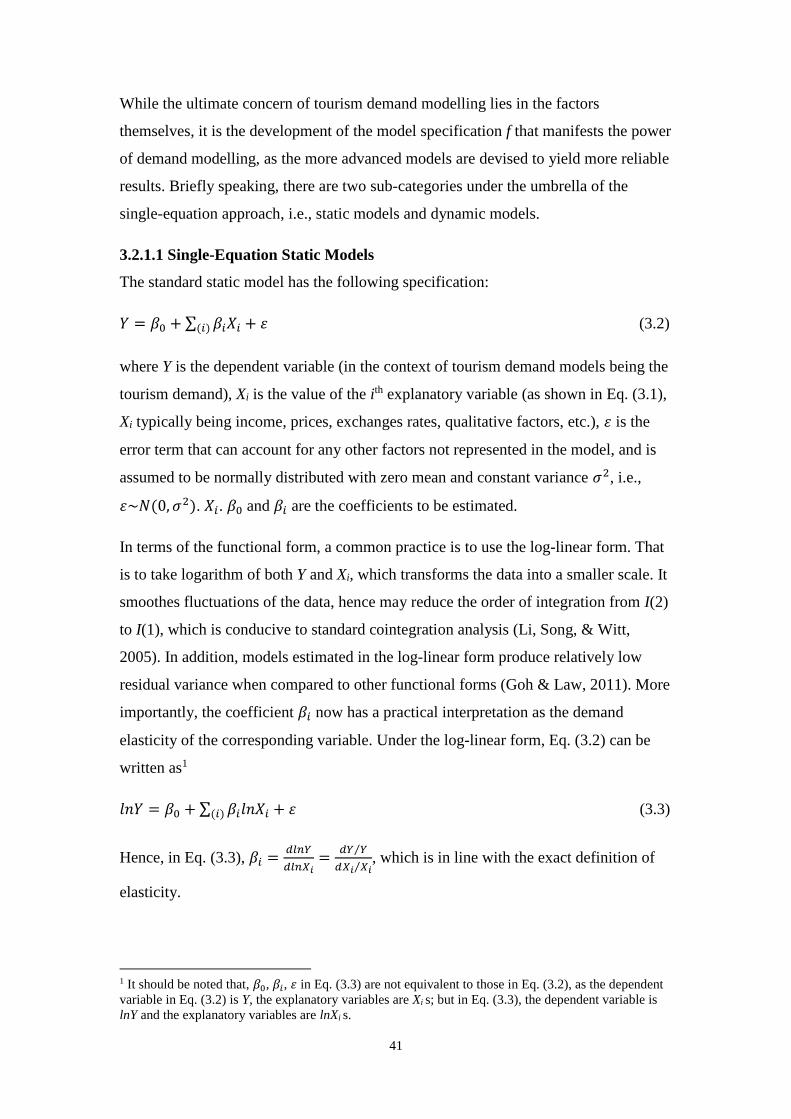
41
While the ultimate concern of tourism demand modelling lies in the factors
themselves, it is the development of the model specification f that manifests the power
of demand modelling, as the more advanced models are devised to yield more reliable
results. Briefly speaking, there are two sub-categories under the umbrella of the
single-equation approach, i.e., static models and dynamic models.
3.2.1.1 Single-Equation Static Models
The standard static model has the following specification:
𝑌 = 𝛽0 +∑ 𝛽𝑖𝑋𝑖(𝑖) + 휀 (3.2)
where Y is the dependent variable (in the context of tourism demand models being the
tourism demand), Xi is the value of the ith explanatory variable (as shown in Eq. (3.1),
Xi typically being income, prices, exchanges rates, qualitative factors, etc.), 휀 is the
error term that can account for any other factors not represented in the model, and is
assumed to be normally distributed with zero mean and constant variance 𝜎2, i.e.,
휀~𝑁(0, 𝜎2). 𝑋𝑖. 𝛽0 and 𝛽𝑖 are the coefficients to be estimated.
In terms of the functional form, a common practice is to use the log-linear form. That
is to take logarithm of both Y and Xi, which transforms the data into a smaller scale. It
smoothes fluctuations of the data, hence may reduce the order of integration from I(2)
to I(1), which is conducive to standard cointegration analysis (Li, Song, & Witt,
2005). In addition, models estimated in the log-linear form produce relatively low
residual variance when compared to other functional forms (Goh & Law, 2011). More
importantly, the coefficient 𝛽𝑖 now has a practical interpretation as the demand
elasticity of the corresponding variable. Under the log-linear form, Eq. (3.2) can be
written as1
𝑙𝑛𝑌 = 𝛽0 +∑ 𝛽𝑖𝑙𝑛𝑋𝑖(𝑖) + 휀 (3.3)
Hence, in Eq. (3.3), 𝛽𝑖 =𝑑𝑙𝑛𝑌
𝑑𝑙𝑛𝑋𝑖=
𝑑𝑌 𝑌⁄
𝑑𝑋𝑖 𝑋𝑖⁄, which is in line with the exact definition of
elasticity.
1 It should be noted that, 𝛽0, 𝛽𝑖, 휀 in Eq. (3.3) are not equivalent to those in Eq. (3.2), as the dependent
variable in Eq. (3.2) is Y, the explanatory variables are Xi s; but in Eq. (3.3), the dependent variable is
lnY and the explanatory variables are lnXi s.

42
Given the advantages, the predominance of log-linear models in tourism demand
studies has been observed over the last few decades (Goh & Law, 2011; Li, Song, &
Witt, 2005; Sinclair, Black, & Sugiyarto, 2003).
The ease of implementation of the static model renders the model a handy tool for
modelling purposes. Many early tourism demand models, such as Gray (1966) and
Artus (1972), were static ones in which the current value of tourism demand is related
only to the current values of explanatory variables (Song, Witt, & Li, 2009, p.48).
Even in the most recent literature, the static model is still being adopted, such as Mao,
Ding, and Lee (2010) and Schiff and Becken (2011).
However, the static models often face criticism for their inherent limitations. In
tourism demand modelling, time series data1 of tourism demand and economic
variables are commonly used. It is assumed that ideally both the dependent variable
(Y) and the explanatory variables (Xi) are stationary, which implies that the mean and
variance of the series do not change over time, so that the linear relationship modelled
is valid for the sample period. A practice based on this assumption is the Engle and
Granger two-stage cointegration analysis, in which the first stage requires estimation
of a static model to capture the long-run equilibrium relationship between variables
(Song & Witt, 2003; Song, Witt, & Li, 2009, pp.90-91). But this assumption can be
restrictive, especially when the data cover a long period of time, as structural change
is possible at some point. Moreover, the error term (휀) in static tourism demand
models has generally been found to be highly autocorrelated (Song, Witt, & Li, p.48).
Autocorrelation indicates that there is correlation between values of the same series at
different times. As a result of autocorrelation, the standard deviation of the estimated
coefficients will be biased, which leads to bias in t-statistics as well as other crucial
statistical indictors (Stock & Watson, 2012, pp.368-369). Another concern indicated
by the high autocorrelation is spurious regression (Goh & Law, 2011; Song, Witt, &
Li, 2009, p.48), which describes that high R-square may wrongly indicate a causal
relationship while in fact Y and Xi are independent of each other. This can often
happen when both the dependent variable and the explanatory variables are integrated,
1 Time series is a sequence of data points observed within a certain period at particular time intervals.
For example, a country’s GDP data over a ten-year period at annual or quarterly frequency.

43
or plainly speaking follow some other underlying trends; but the dependent variable
and explanatory variables themselves do not have any relationship.
In an attempt to solve the problems with static models, dynamic effects, such as the
lagged value of the dependent and explanatory variables, were introduced into tourism
demand models (Song, Witt, & Li, 2009, p.48). This leads to the development of
dynamic models.
3.2.1.2 Single-Equation Dynamic Models
It is believed that dynamic models are more realistic, because they take account of the
lagged effect of explanatory variables, rather than simply the instantaneous effect
(Goh & Law, 2011). The inclusion of lagged variables as regressors, while in the first
place has to do with solving the problems inherent in static models, has also strong
economic justifications. As summarised by Morley (2009), these are:
lags in implementing a decision to travel (for example, making travel
decisions in advance)
information lags (for example, using historical prices to anticipate the costs of
living at destination)
as a way of recognising supply rigidities
to account for long-term adjustment dynamics
word-of-mouth recommendations (for example, influenced by a previous
visitor) and
repeat visitors.
In practice, the above justifications suggest that both the lagged values of the
dependent variable and those of the explanatory variables appear in a dynamic model.
Autoregressive Distributed Lag Model (ADLM)
The Model
By including the lagged dependent and explanatory variables, the standard static
model Eq. (3.2) can be extended into the following specification, which is the general
form of an autoregressive distributed lag model (ADLM)
𝑌𝑡 = 𝛽0 + ∑ ∑ 𝛽𝑖𝑗𝑋𝑖,𝑡−𝑗𝑝𝑗=0
𝑘𝑖=1 + ∑ 𝜆𝑗𝑌𝑡−𝑗
𝑞𝑗=1 + 휀𝑡 (3.4)

44
where t denotes the time or period of data; j indices time lags, and up to p and q lags;
k is the number of explanatory variables 𝑋𝑖; 𝜆𝑗 is the coefficient on 𝑌𝑡−𝑗 and needs to
be estimated (Morley, 2009; Song, Witt, & Li, 2009, p.47). The rest of the notation
has the same meaning as that of Eq. (3.2). The model can also be more specifically
called ADLM (p, q). To determine the lag length p (or q), a general guide is that p=1
for annual data, p=4 for quarterly data, p=6 for bimonthly data, and p=12 for monthly
data. A more scientific determination can be based on the Akaike information
criterion (AIC) or Schwarz information criterion (SBC) (Song, Witt, & Li, 2009,
p.42).
Model Estimation: General-to-Specific Approach
The estimation of Eq. (3.4) can follow one of the two strategies: simple-to-general
approach and general-to-specific approach. The simple-to-general approach starts
with a relatively simple specification (usually a low lag length p), then the model is
re-specified by introducing new explanatory variables or higher order of lags if the
residuals of the simple specification exhibit heteroscedasticity, autocorrelation or lack
of normality. The final model may be achieved until the re-specified model is
theoretically sound and statistically acceptable (Song, Witt, & Li, 2009, p.47). The
simple-to-general approach is often criticised for its excessive data mining, as
different researchers may obtain different model specifications based on the same data
set (Song & Witt, 2003).
Alternatively, the general-to-specific approach can be followed, which is a ‘top-
down’ modelling strategy. It starts with a general model which contains as many
variables suggested by economic theory as possible. The general model is then
estimated to see whether all the variables included are statistically significant or not.
The next step is to eliminate the least significant variable according to the t-statistics.
With one less variable now, the model is re-estimated and the elimination process is
carried out until a statistically acceptable specification with ‘correct’ signs of
coefficients predicted by economic theory is reached (Song, Wong, & Chon, 2003). It
should be noted that, sign changes of coefficients and varying estimation of
coefficients can be observed during the course of variable elimination. This may
indicate that the estimates are not very robust. It may be related to the suppression
effect where the correlationship between variables is changed by suppressor. Hence,
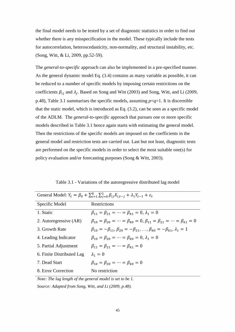
45
the final model needs to be tested by a set of diagnostic statistics in order to find out
whether there is any misspecification in the model. These typically include the tests
for autocorrelation, heteroscedasticity, non-normality, and structural instability, etc.
(Song, Witt, & Li, 2009, pp.52-59).
The general-to-specific approach can also be implemented in a pre-specified manner.
As the general dynamic model Eq. (3.4) contains as many variable as possible, it can
be reduced to a number of specific models by imposing certain restrictions on the
coefficients 𝛽𝑖𝑗 and 𝜆𝑗. Based on Song and Witt (2003) and Song, Witt, and Li (2009,
p.48), Table 3.1 summarises the specific models, assuming p=q=1. It is discernible
that the static model, which is introduced as Eq. (3.2), can be seen as a specific model
of the ADLM. The general-to-specific approach that pursues one or more specific
models described in Table 3.1 hence again starts with estimating the general model.
Then the restrictions of the specific models are imposed on the coefficients in the
general model and restriction tests are carried out. Last but not least, diagnostic tests
are performed on the specific models in order to select the most suitable one(s) for
policy evaluation and/or forecasting purposes (Song & Witt, 2003).
Table 3.1 - Variations of the autoregressive distributed lag model
General Model: 𝑌𝑡 = 𝛽0 + ∑ ∑ 𝛽𝑖𝑗𝑋𝑖,𝑡−𝑗1𝑗=0
𝑘𝑖=1 + 𝜆1𝑌𝑡−1 + 휀𝑡
Specific Model Restrictions
1. Static 𝛽11 = 𝛽21 = ⋯ = 𝛽𝑘1 = 0, 𝜆1 = 0
2. Autoregressive (AR) 𝛽10 = 𝛽20 = ⋯ = 𝛽𝑘0 = 0, 𝛽11 = 𝛽21 = ⋯ = 𝛽𝑘1 = 0
3. Growth Rate 𝛽10 = −𝛽11, 𝛽20 = −𝛽21, …, 𝛽𝑘0 = −𝛽𝑘1, 𝜆1 = 1
4. Leading Indicator 𝛽10 = 𝛽20 = ⋯ = 𝛽𝑘0 = 0, 𝜆1 = 0
5. Partial Adjustment 𝛽11 = 𝛽21 = ⋯ = 𝛽𝑘1 = 0
6. Finite Distributed Lag 𝜆1 = 0
7. Dead Start 𝛽10 = 𝛽20 = ⋯ = 𝛽𝑘0 = 0
8. Error Correction No restriction
Note: The lag length of the general model is set to be 1.
Source: Adapted from Song, Witt, and Li (2009, p.48).
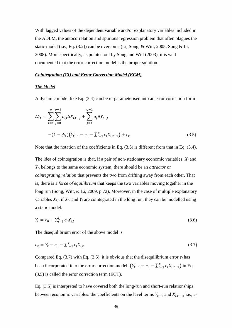
46
With lagged values of the dependent variable and/or explanatory variables included in
the ADLM, the autocorrelation and spurious regression problem that often plagues the
static model (i.e., Eq. (3.2)) can be overcome (Li, Song, & Witt, 2005; Song & Li,
2008). More specifically, as pointed out by Song and Witt (2003), it is well
documented that the error correction model is the proper solution.
Cointegration (CI) and Error Correction Model (ECM)
The Model
A dynamic model like Eq. (3.4) can be re-parameterised into an error correction form
∆𝑌𝑡 =∑∑𝑏𝑖𝑗∆𝑋𝑖,𝑡−𝑗
𝑝−1
𝑗=0
𝑘
𝑖=1
+∑𝑎𝑗∆𝑌𝑡−𝑗
𝑞−1
𝑗=1
−(1 − 𝜙1)(𝑌𝑡−1 − 𝑐0 − ∑ 𝑐𝑖𝑋𝑖,𝑡−1𝑘𝑖=1 ) + 휀𝑡 (3.5)
Note that the notation of the coefficients in Eq. (3.5) is different from that in Eq. (3.4).
The idea of cointegration is that, if a pair of non-stationary economic variables, Xt and
Yt, belongs to the same economic system, there should be an attractor or
cointegrating relation that prevents the two from drifting away from each other. That
is, there is a force of equilibrium that keeps the two variables moving together in the
long run (Song, Witt, & Li, 2009, p.72). Moreover, in the case of multiple explanatory
variables Xi,t, if Xi,t and Yt are cointegrated in the long run, they can be modelled using
a static model:
𝑌𝑡 = 𝑐0 + ∑ 𝑐𝑖𝑋𝑖,𝑡𝑘𝑖=1 (3.6)
The disequilibrium error of the above model is
𝑒𝑡 = 𝑌𝑡 − 𝑐0 − ∑ 𝑐𝑖𝑋𝑖,𝑡𝑘𝑖=1 (3.7)
Compared Eq. (3.7) with Eq. (3.5), it is obvious that the disequilibrium error et has
been incorporated into the error correction model. (𝑌𝑡−1 − 𝑐0 − ∑ 𝑐𝑖𝑋𝑖,𝑡−1𝑘𝑖=1 ) in Eq.
(3.5) is called the error correction term (ECT).
Eq. (3.5) is interpreted to have covered both the long-run and short-run relationships
between economic variables: the coefficients on the level terms 𝑌𝑡−1 and 𝑋𝑖,𝑡−1, i.e., c0

47
and ci, are related to the long-run demand elasticities whereas the coefficients on the
first differenced terms ∆𝑌𝑡−𝑗 and ∆𝑋𝑖,𝑡−𝑗, i.e., aj and bij, reflect the short-run
dynamics. The term −(1 − 𝜙1)(𝑌𝑡−1 − 𝑐0 − ∑ 𝑐𝑖𝑋𝑖,𝑡−1𝑘𝑖=1 ) represents the error
correction mechanism. 𝜙1 is a positive number between 0 and 1. Therefore the
coefficient −(1 − 𝜙1) is between -1 and 0, which means the system will adjust itself
towards equilibrium by removing (1 − 𝜙1) of a unit from the error made in the
previous period (Smeral, 2010; Song, Witt, & Li, 2009, p.89). The larger the
(1 − 𝜙1), the faster the adjustment is.
Model Estimation
The estimation of an ECM typically starts with deciding the order of integration of the
variables, using the unit root tests such as Augmented Dickey-Fuller (ADF) tests,
Phillips-Perron (PP) tests and Kwiatkowski, Phillips, Schmidt, and Shin (KPSS) tests.
The order of integration of a time series reports the minimum number of differences
required to obtain a stationary series. For example, if no difference is needed and the
series is stationary itself, the order of integration is zero, or the series follows an I(0)
process. If the series is differenced once to become stationary, then it follows an I(1)
process, and it is said the series contains a unit root. For a cointegrating relation to be
detected, all the variables concerned should be integrated of order one, i.e., I(1) (Song,
Witt, & Li, 2009, p.84). Therefore, unit root tests are essential to decide whether an
ECM can be implemented for modelling purposes.
After the unit root tests, the coefficients of the ECM can be estimated following
different procedures. Briefly speaking, these include the Engle-Granger two-stage
approach, the Wickens-Breusch (WB) one-stage approach, the Pesaran, Shin, and
Smith ADLM bounds testing approach and the Johansen maximum likelihood (JML)
approach (Halicioglu, 2010; Song & Lin, 2010; Song, Witt, & Li, 2003; Song, Witt,
& Li, 2009, pp.90-93).
The Engle-Granger approach involves first testing for a cointegrating relation based
on the static long-run equilibrium regression, i.e., Eq. (3.6). If the estimated residual
term (or error correction term) Eq. (3.7) is stationary, then the cointegrating relation is
accepted. In the second stage the ECM is estimated, with the error correction term
coming from the first stage included. As opposed to the Engle-Granger approach,

48
which may be biased in small samples (Song, Witt, & Li, 2009, p.91), the Wickens-
Breusch (WB) approach directly estimates the ECM in one step, without explicitly
accounting for the cointegrating relation:
∆𝑌𝑡 = 𝑏0 + ∑ ∑ 𝑏𝑖𝑗∆𝑋𝑖,𝑡−𝑗𝑝−1𝑗=0
𝑘𝑖=1 + ∑ 𝑎𝑗∆𝑌𝑡−𝑗
𝑞−1𝑗=1 + 𝜆0𝑌𝑡−1 + ∑ 𝜆𝑖𝑋𝑖,𝑡−1
𝑘𝑖=1 + 휀𝑡 (3.8)
A more recent development in the ECM estimation field is the Pesaran, Shin, and
Smith ADLM bounds testing approach (Pesaran, Shin, & Smith, 2001). It has been
extensively used in most of the recent studies that adopted the ECM, for example
Halicioglu (2010), Onafowora and Owoye (2012), Song, Gartner, and Tasci (2012),
Song, Lin, Witt, and Zhang (2011), and Wang (2009). The advantage of this approach
is its ability to detect cointegrating relation and solve the small sample problem
irrespective of whether the dependent and independent variables are purely I(1),
purely I(0), or a mixture of both (Song, Gartner, & Tasci, 2012; Wang, 2009). Rather
than using a new specification, the bounds testing approach basically follows Eq.
(3.8), and finishes the estimation in one step. The bounds testing is based on an F-test
performed on the level terms in Eq. (3.8). Specifically, the null hypothesis (H0: 𝜆0 =
𝜆1 = ⋯ = 𝜆𝑘 = 0) states that there is no cointegration among the variables, whereas
the alternative hypothesis (at least one of 𝜆𝑖 is non zero) suggests there exists
cointegration. The F-statistic is then compared with two sets of critical values
reported in Pesaran, Shin, and Smith (2001). If the F-statistic exceeds the upper
critical bounds value, then H0 is rejected, indicating there is a cointegrating relation. If
the F-statistic falls below the lower critical bounds value, then H0 is accepted and no
integration is found. If the F-statistic lies between the upper and lower bounds value,
then it is inclusive regarding the existence of cointegration (Halicioglu, 2010;
Onafowora & Owoye, 2012). Moreover, if H0 (𝜆0 = 𝜆1 = ⋯ = 𝜆𝑘 = 0) is rejected, a
further t-test is often used to confirm the existence of cointegration (Seetaram, Song,
& Page, 2013; Song, Gartner, & Tasci, 2012; Song & Lin, 2010). This t-test is
performed on the coefficient on the lagged level term of the dependent variable 𝑌𝑡−1,
i.e., 𝜆0. Again, the t-test assumes the null hypothesis of no cointegration (H0: 𝜆0 = 0)
with respect to the tourism demand. Pesaran, Shin, and Smith (2001) generated the
upper bounds and lower bounds values for this t-test, and the interpretation is similar
to that for the F-test.

49
Another popular estimation procedure of ECM is the Johansen maximum likelihood
(JML) approach. It is, however, based on a different modelling framework, i.e.,
system-of-equations. For the Engle-Granger approach, the WB approach and the
bounds testing approach, the detection of cointegration is based on a single equation,
which implicitly assumes that there is only one cointegrating relation among all the
variables. In contrast, the JML approach allows for multiple cointegrating relations,
and subsequently multiple ECMs can be obtained (Song, Witt, & Li, 2003).
Discussions on the JML approach will be followed in Section 3.2.2.1.
3.2.1.3 Applications and Limitations
Elasticity Analysis: Point Estimates versus Intervals
Based on the coefficients estimated from the single-equation models (static models,
dynamic models such as ADLM and ECM), it is a common practice to derive both the
long-run and short-run demand elasticities, which measure the responsiveness of
tourism demand towards one unit change in specified influencing factors, i.e., 𝑑𝑌 𝑌⁄
𝑑𝑋𝑖 𝑋𝑖⁄.
As there is one set of coefficients yielded from the estimation, only point estimates of
elasticities can be derived accordingly. This poses two limitations that concern the
researchers. The first is that the elasticities are assumed to be time-invariant. That is,
over the whole sample period tourism demand will increase/decrease in response to
say, one unit change in tourists’ income, by the same percentage. This assumption is
very rigid. As argued by Song, Witt, and Li (2009, p.138), the parameters of the
demand model may vary over time, due to structural instability in the underlying data
generating process. Such structural change is mainly related to important social,
political and economic policy changes. To relax the constancy restriction on the
parameters to be estimated in a traditional fixed-parameter econometric model, an
advance called the time-varying-parameter (TVP) model has been adopted (Li, Wong,
Song, & Witt, 2006; Song, Witt, & Li, 2009, pp.138-148). Discussions will follow in
Section 3.2.3. The second limitation of point estimates is that the single value of
elasticity is not informative enough to assess whether it is statistically significant and
whether it truly represents elastic demand. The reasons are that there is no information
about the degree of variability; elasticity is often a non-linear function of other
parameters; the sampling distribution of a point elasticity estimator is likely to follow
a non-normal distribution, which renders conventional statistical inference based on

50
normal approximation problematic (Song, Kim, & Yang, 2010). To overcome the
second limitation, it is argued that a confidence interval of the elasticity will be more
useful, and some recent studies, such as Otero-Giráldez, Álvarez-Díaz, and González-
Gómez (2012), Song, Kim, and Yang (2010) and Song and Lin (2010), have followed
this practice.
Applications
As noted at the beginning of Section 3.2, the econometric tourism demand models aim
to build a causal link between tourism demand and its influencing factors. That is,
trying to account for the variations of tourism demand1 with a range of factors. To this
end, the single-equation approach (both the static models and the dynamic models)
offers a tractable solution, as variables are arranged in a clear-cut manner and the
implementation of estimation is straightforward. Therefore, the single-equation
approach of modelling has been extensively applied in the tourism demand studies
since the very earliest days (e.g., Artus, 1972; Gray, 1966), and this trend can still be
observed.
Given its tractability, the applications of the single-equation approach (static and
dynamic) are versatile. A major strand of studies is centred on identifying the
influencing factors and quantifying their effects on tourism demand. Much of the
attention has been paid to economic factors, such as income, prices and exchange
rates (e.g., Smeral, 1988; Song, Witt, & Li, 2003; Song, Wong, & Chon, 2003). A less
often considered but recurrent factor is marketing expenditures (Crouch, Schultz, &
Valerio, 1992; Lim, 1997; Song, Witt, & Li, 2009, p.30), which appeared in the
literature as early as 1980s (Stabler, Papatheodorou, & Sinclair, 2010, p.58).
Accompanying the modelling exercise, demand elasticities are generally derived for
analysis purposes. For example, the marketing expenditure elasticity can be used as an
indication of how successful the marketing campaigns of a destination are (Kulendran
& Dwyer, 2009; Zhang, Kulendran, & Song, 2010). More recently, research has been
extended to quantifying the effect of non-economic factors, such as meteorological
1 Tourism demand is often observed within a certain time frame, and the data on tourism demand are
mostly time series. Hence the focus of tourism demand modelling is mainly on the variation of demand
over time. Nevertheless, the spatial dimension of tourism demand attracts sufficient attention too.
Spatial models are developed to account for the difference of tourism demand between destinations.

51
factors (e.g., Goh, 2012; Otero-Giráldez, Álvarez-Díaz, & González-Gómez, 2012)
and media messages (Stepchenkova & Eales, 2011).
Apart from identifying the influencing factors, another strand of studies places the
emphasis on the impact of special events or policies. Some of the analyses rely on
dummy variables in the model. The logic is that the coefficients on dummy variables
represent the difference of tourism demand between the scenario where no special
event/policy takes place and the scenario where the event/policy occurs. Examples
following this logic are Song, Gartner and Tasci (2012), which estimated the loss of
China’s tourism industry due to visa restrictions imposed on international visitors, and
Wang (2009), which calculated the impacts of a series of natural and economic crises
on Taiwan’s inbound tourism. Some other studies based the analysis on generic
economic variables. One way is to include new variable(s). For example, Seetaram,
Song, and Page (2013) included a tax variable in an ADLM and estimated the demand
elasticity on Air Passenger Duty (APD), in order to analyse the sensitivity of UK’s
outbound tourism towards policy changes in tourism taxes. Another way is to use
third-party forecasts of economic variables (such as IMF, UNWTO) to generate
forecasts of tourism demand. As the third-party forecasts have already incorporated
information about the special event/policy, the forecasts of tourism demand would
thus be able to reflect the influence of the event/policy. Examples are the studies by
Smeral (2010), Song and Lin (2010), Song, Lin, Witt, and Zhang (2011), which aimed
to gauge the impacts of the worldwide economic crisis since 2008.
Limitations: the Assumption of Exogeneity
Despite their versatile capabilities, the single-equation econometric models are not
without problem. Fundamental limitations of the single-equation approach are often
the target of criticism.
As pointed out by Stabler, Papatheodorou and Sinclair (2010, p.59), one problem that
the approach faces is that explanatory variables are often selected on a fairly ad hoc
basis. This will result in misspecification of the equation and biased estimation. In a
tourism demand model, apart from the factors that have been justified by relevant
economic theory (i.e., tourists’ income level, relative prices in the destination
concerned and in substitute destinations, exchange rates), there are often other specific
factors being considered, such as marketing expenditure, monetary supply, and even

52
immigration crime rate (Li, Song, & Witt, 2005). Although the general-to-specific
procedure (Song, Witt, & Li, 2009, pp.46-69) can help to exclude those that are
irrelevant, the question still remains that how well justified it is to include certain
variables. After all, the inclusion is largely dictated by the theme of the research rather
than by rigorous theory. The model itself does not judge the appropriateness of the
variables appearing in it.
A more fundamental concern of the single-equation approach is about its assumption
of exogeneity, which requires all the explanatory variables to be decided by factors
outside the model. As such, any randomness in the data generating process (DGP) of
the explanatory variables is independent of the error term in the DGP for the
dependent variable (Davidson & Mackinnon, 2003, p.89). Take the simplest
univariate static regression as an example,
𝑌𝑖 = 𝛽0 + 𝛽1𝑋𝑖 + 𝑢𝑖 , 𝑖 = 1,… , 𝑛 (3.9)
the exogeneity means
𝐸(𝑢𝑖|𝑋𝑖) = 0 (3.10)
Correspondingly, if the explanatory variables and the error term are not independent,
i.e., 𝑐𝑜𝑣(𝑋𝑖, 𝑢𝑖) ≠ 0,then the explanatory variables are said to be endogenous.
The exogeneity assumption is of utmost importance to the single-equation approach,
because the breach of Eq. (3.10) will result in biased ordinary-least-square (OLS)
estimation (Davidson & Mackinnon, 2003, pp.88-90).
As discussed by Stock and Watson (2012, p.462), the breach of Eq. (3.10) (i.e.,
existence of correlation between 𝑋𝑖 and 𝑢𝑖) can stem from omitted variables,
measurement errors in the regressors, and simultaneous causality. While the former
two sources cannot be completely avoided even with other modelling approaches, the
latter one tends to plague the single-equation approach more. Simultaneous causality
is a situation where the causality runs not only from the explanatory variables to the
dependent variable (i.e., 𝑋𝑖 causes 𝑌𝑖), but also in the reverse direction (i.e., 𝑌𝑖 causes
𝑋𝑖). Put it in the context of tourism demand modelling, simultaneous causality implies
that not only the tourism demand for destination j is influenced by the prices in
destination j and the origin country i’s income level, but also the tourism demand can
53
have feedback impact on j’s local prices and even country i’s income level. In reality,
it is not uncommon to see the influx of tourists has caused demand pressure on
destination’s local economy. For example, using the data for 45 European cities,
Albalate and Bel (2010) find that the additional demand for public transport by
tourists imposed external costs on local residents due to the congestion caused by a
supply constraint, even though the tourism receipts could provide some additional
funding for the transport services. In the same vein, the demand pressure can be
extended to affect generic goods/services and result in inflation (i.e., price increase) in
a local economy, especially when the supplies are not perfectly elastic to meet the
demand. Therefore, the feedback impact of tourism demand on its economic
determinants is an important dimension of tourism demand modelling, which in fact
has often been overlooked. Few studies using the single-equation approach to
modelling have tried to account for the simultaneous causality between tourism
demand and its influencing factors, or even mention the limitations of the single-
equation approach.
3.2.2 The System-of-Equations Approach
In view of the limitations of the single-equation approach, mainly the ad hoc model
specification and the exogeneity assumption, systems of equations have been put
forward and adopted in tourism demand modelling.
There are three major types of models, which are the vector autoregressive (VAR)
model, the almost ideal demand system (AIDS), and the panel data analysis model.
Just like the single-equation approach, all the three types of systems of equations can
also accommodate the dynamic features of tourism demand. Although the
specifications of the three types of systems can be distinctly different, the backbone of
them (that is the individual equation in it) is just similar to Eq. (3.2) for a static
specification, and Eq. (3.4) and Eq. (3.5) for a dynamic form.
3.2.2.1 Vector Autoregressive (VAR) Model
The Model
The development of the vector autoregressive (VAR) model mainly aims to relax the
assumption of exogeneity that is implicitly imposed on the single-equation models. To
allow for endogeneity in the model, it was popular to use the simultaneous-equation
approaches within the context of structural macroeconomic modelling, which dated

54
back to the 1950s and 1960s (Song & Witt, 2006). These approaches often required a
priori restrictions to be imposed on the parameters of the equations. Many of the
restrictions, as argued by Sims (1980), were ‘incredible’. In order to bypass the need
of structural modelling (i.e., one that depends on the imposition of incorrect prior
information), Sims developed a VAR model that treated all variables as endogenous,
except for the deterministic variables such as trend, intercept and dummy variables
(Song & Witt, 2006). A general VAR(p) model, where p is the lag length, can be
written as
𝒀𝑡 = ∑ 𝑨𝑙𝒀𝑡−𝑙𝑝𝑙=1 + 𝑪0 + 𝑪1𝑡 + 𝑼𝑡 (3.11)
𝑼𝑡~𝐼𝐼𝐷(𝟎, 𝚺) (3.12)
where 𝒀𝑡 is a 𝑘 × 1 vector of endogenous variables, 𝑨𝑙 is a 𝑘 × 𝑘 matrix of
coefficients to be estimated, 𝑪0 is a 𝑘 × 1 vector of intercepts, 𝑪1 is a 𝑘 × 1 vector of
coefficients on the trend, 𝑼𝑡 is a 𝑘 × 1 vector of innovations or shocks. In addition,
dummy variables can also be added to Eq. (3.11) in the same manner as the trend
terms. Hence, there are in total k equations to be estimated. Assuming 𝑼𝑡 to be
contemporaneously correlated but not autocorrelated, each equation in the system can
be individually estimated with OLS estimator or the seemingly unrelated regression
estimator (SURE) (Song & Witt, 2006).
The variables in 𝒀𝑡 are endogenous variables (either justified by theory, or simply due
to lack of evidence of exogeneity) in a system, which implies that one variable can
correlate with one or some of the rest of the variables. The idea of VAR model is that
each variable in 𝒀𝑡 is regressed on its lags and all other endogenous variables. Hence,
for each variable, there is a unique equation capturing the causal relationship running
from the rest of the endogenous variables to the variable itself. In the context of
tourism demand modelling, the vector 𝒀𝑡 typically include, as in Eq. (3.1), the tourism
demand variable, the price variables of the destination concerned as well as those of
the competing destinations, the exchange rate variables and the travel cost variables1.
More generally, the VAR model can be extended to include exogenous variables
1 The inclusion of non-economic factors as endogenous variables is rare and has to be taken with
caution. Deterministic variables such as trend, seasonality and dummy variables typically enter a VAR
system as exogenous variables.
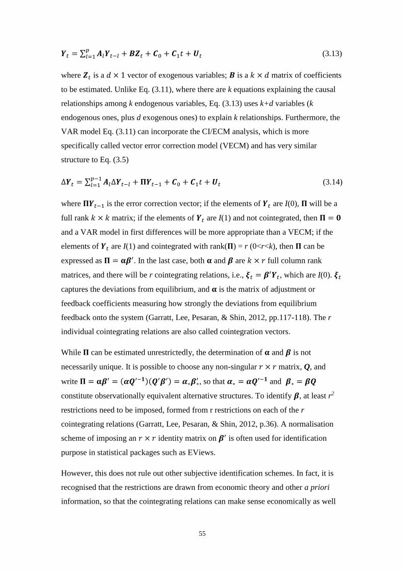
55
𝒀𝑡 = ∑ 𝑨𝑙𝒀𝑡−𝑙𝑝𝑙=1 + 𝑩𝒁𝑡 + 𝑪0 + 𝑪1𝑡 + 𝑼𝑡 (3.13)
where 𝒁𝑡 is a 𝑑 × 1 vector of exogenous variables; 𝑩 is a 𝑘 × 𝑑 matrix of coefficients
to be estimated. Unlike Eq. (3.11), where there are k equations explaining the causal
relationships among k endogenous variables, Eq. (3.13) uses k+d variables (k
endogenous ones, plus d exogenous ones) to explain k relationships. Furthermore, the
VAR model Eq. (3.11) can incorporate the CI/ECM analysis, which is more
specifically called vector error correction model (VECM) and has very similar
structure to Eq. (3.5)
∆𝒀𝑡 = ∑ 𝑨𝑙∆𝒀𝑡−𝑙𝑝−1𝑙=1 + 𝚷𝒀𝑡−1 + 𝑪0 + 𝑪1𝑡 + 𝑼𝑡 (3.14)
where 𝚷𝒀𝑡−1 is the error correction vector; if the elements of 𝒀𝑡 are I(0), 𝚷 will be a
full rank 𝑘 × 𝑘 matrix; if the elements of 𝒀𝑡 are I(1) and not cointegrated, then 𝚷 = 𝟎
and a VAR model in first differences will be more appropriate than a VECM; if the
elements of 𝒀𝑡 are I(1) and cointegrated with rank(𝚷) = r (0<r<k), then 𝚷 can be
expressed as 𝚷 = 𝛂𝜷′. In the last case, both 𝛂 and 𝜷 are 𝑘 × 𝑟 full column rank
matrices, and there will be r cointegrating relations, i.e., 𝝃𝑡 = 𝜷′𝒀𝑡, which are I(0). 𝝃𝑡
captures the deviations from equilibrium, and 𝛂 is the matrix of adjustment or
feedback coefficients measuring how strongly the deviations from equilibrium
feedback onto the system (Garratt, Lee, Pesaran, & Shin, 2012, pp.117-118). The r
individual cointegrating relations are also called cointegration vectors.
While 𝚷 can be estimated unrestrictedly, the determination of 𝛂 and 𝜷 is not
necessarily unique. It is possible to choose any non-singular 𝑟 × 𝑟 matrix, Q, and
write 𝚷 = 𝛂𝜷′ = (𝜶𝑸′−𝟏)(𝑸′𝜷′) = 𝜶∗𝜷∗′ , so that 𝜶∗ = 𝜶𝑸′−𝟏 and 𝜷∗ = 𝜷𝑸
constitute observationally equivalent alternative structures. To identify 𝜷, at least r2
restrictions need to be imposed, formed from r restrictions on each of the r
cointegrating relations (Garratt, Lee, Pesaran, & Shin, 2012, p.36). A normalisation
scheme of imposing an 𝑟 × 𝑟 identity matrix on 𝜷′ is often used for identification
purpose in statistical packages such as EViews.
However, this does not rule out other subjective identification schemes. In fact, it is
recognised that the restrictions are drawn from economic theory and other a priori
information, so that the cointegrating relations can make sense economically as well
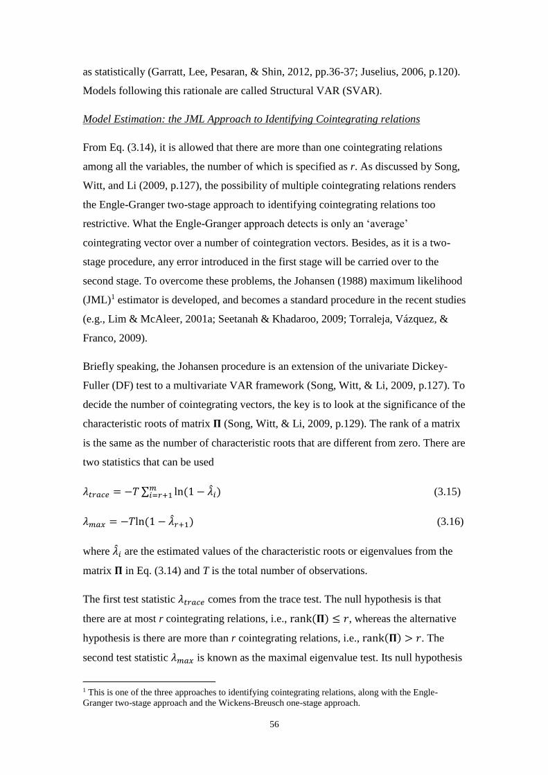
56
as statistically (Garratt, Lee, Pesaran, & Shin, 2012, pp.36-37; Juselius, 2006, p.120).
Models following this rationale are called Structural VAR (SVAR).
Model Estimation: the JML Approach to Identifying Cointegrating relations
From Eq. (3.14), it is allowed that there are more than one cointegrating relations
among all the variables, the number of which is specified as r. As discussed by Song,
Witt, and Li (2009, p.127), the possibility of multiple cointegrating relations renders
the Engle-Granger two-stage approach to identifying cointegrating relations too
restrictive. What the Engle-Granger approach detects is only an ‘average’
cointegrating vector over a number of cointegration vectors. Besides, as it is a two-
stage procedure, any error introduced in the first stage will be carried over to the
second stage. To overcome these problems, the Johansen (1988) maximum likelihood
(JML)1 estimator is developed, and becomes a standard procedure in the recent studies
(e.g., Lim & McAleer, 2001a; Seetanah & Khadaroo, 2009; Torraleja, Vázquez, &
Franco, 2009).
Briefly speaking, the Johansen procedure is an extension of the univariate Dickey-
Fuller (DF) test to a multivariate VAR framework (Song, Witt, & Li, 2009, p.127). To
decide the number of cointegrating vectors, the key is to look at the significance of the
characteristic roots of matrix 𝚷 (Song, Witt, & Li, 2009, p.129). The rank of a matrix
is the same as the number of characteristic roots that are different from zero. There are
two statistics that can be used
𝜆𝑡𝑟𝑎𝑐𝑒 = −𝑇∑ ln(1 − �̂�𝑖)𝑚𝑖=𝑟+1 (3.15)
𝜆𝑚𝑎𝑥 = −𝑇ln(1 − �̂�𝑟+1) (3.16)
where �̂�𝑖 are the estimated values of the characteristic roots or eigenvalues from the
matrix 𝚷 in Eq. (3.14) and T is the total number of observations.
The first test statistic 𝜆𝑡𝑟𝑎𝑐𝑒 comes from the trace test. The null hypothesis is that
there are at most r cointegrating relations, i.e., rank(𝚷) ≤ 𝑟, whereas the alternative
hypothesis is there are more than r cointegrating relations, i.e., rank(𝚷) > 𝑟. The
second test statistic 𝜆𝑚𝑎𝑥 is known as the maximal eigenvalue test. Its null hypothesis
1 This is one of the three approaches to identifying cointegrating relations, along with the Engle-
Granger two-stage approach and the Wickens-Breusch one-stage approach.
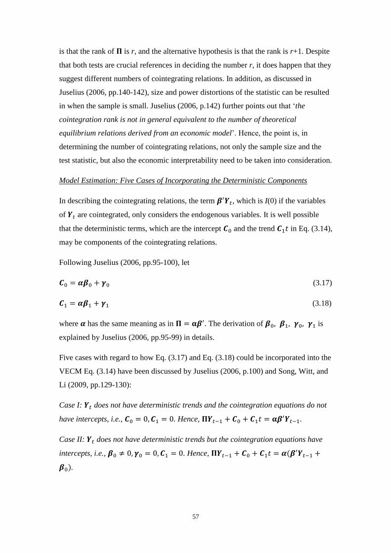
57
is that the rank of 𝚷 is r, and the alternative hypothesis is that the rank is r+1. Despite
that both tests are crucial references in deciding the number r, it does happen that they
suggest different numbers of cointegrating relations. In addition, as discussed in
Juselius (2006, pp.140-142), size and power distortions of the statistic can be resulted
in when the sample is small. Juselius (2006, p.142) further points out that ‘the
cointegration rank is not in general equivalent to the number of theoretical
equilibrium relations derived from an economic model’. Hence, the point is, in
determining the number of cointegrating relations, not only the sample size and the
test statistic, but also the economic interpretability need to be taken into consideration.
Model Estimation: Five Cases of Incorporating the Deterministic Components
In describing the cointegrating relations, the term 𝜷′𝒀𝑡, which is I(0) if the variables
of 𝒀𝑡 are cointegrated, only considers the endogenous variables. It is well possible
that the deterministic terms, which are the intercept 𝑪0 and the trend 𝑪1𝑡 in Eq. (3.14),
may be components of the cointegrating relations.
Following Juselius (2006, pp.95-100), let
𝑪0 = 𝜶𝜷0 + 𝜸0 (3.17)
𝑪1 = 𝜶𝜷1 + 𝜸1 (3.18)
where 𝜶 has the same meaning as in 𝚷 = 𝛂𝜷′. The derivation of 𝜷0, 𝜷1, 𝜸0, 𝜸1 is
explained by Juselius (2006, pp.95-99) in details.
Five cases with regard to how Eq. (3.17) and Eq. (3.18) could be incorporated into the
VECM Eq. (3.14) have been discussed by Juselius (2006, p.100) and Song, Witt, and
Li (2009, pp.129-130):
Case I: 𝒀𝑡 does not have deterministic trends and the cointegration equations do not
have intercepts, i.e., 𝑪0 = 0, 𝑪1 = 0. Hence, 𝚷𝒀𝑡−1 + 𝑪0 + 𝑪1𝑡 = 𝛂𝜷′𝒀𝑡−1.
Case II: 𝒀𝑡 does not have deterministic trends but the cointegration equations have
intercepts, i.e., 𝜷0 ≠ 0, 𝜸0 = 0, 𝑪1 = 0. Hence, 𝚷𝒀𝑡−1 + 𝑪0 + 𝑪1𝑡 = 𝜶(𝜷′𝒀𝑡−1 +
𝜷0).
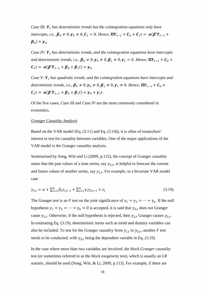
58
Case III: 𝒀𝑡 has deterministic trends but the cointegration equations only have
intercepts, i.e., 𝜷0 ≠ 0, 𝜸0 ≠ 0, 𝑪1 = 0. Hence, 𝚷𝒀𝑡−1 + 𝑪0 + 𝑪1𝑡 = 𝜶(𝜷′𝒀𝑡−1 +
𝜷0) + 𝜸0.
Case IV: 𝒀𝑡 has deterministic trends, and the cointegration equations have intercepts
and deterministic trends, i.e., 𝜷0 ≠ 0, 𝜸0 ≠ 0,𝜷1 ≠ 0, 𝜸1 = 0. Hence, 𝚷𝒀𝑡−1 + 𝑪0 +
𝑪1𝑡 = 𝜶(𝜷′𝒀𝑡−1 + 𝜷0 + 𝜷1𝑡) + 𝜸0.
Case V: 𝒀𝑡 has quadratic trends, and the cointegration equations have intercepts and
deterministic trends, i.e., 𝜷0 ≠ 0, 𝜸0 ≠ 0,𝜷1 ≠ 0, 𝜸1 ≠ 0. Hence, 𝚷𝒀𝑡−1 + 𝑪0 +
𝑪1𝑡 = 𝜶(𝜷′𝒀𝑡−1 + 𝜷0 + 𝜷1𝑡) + 𝜸0 + 𝜸1𝑡.
Of the five cases, Case III and Case IV are the most commonly considered in
economics.
Granger Causality Analysis
Based on the VAR model (Eq. (3.11) and Eq. (3.14)), it is often of researchers’
interest to test for causality between variables. One of the major applications of the
VAR model is the Granger causality analysis.
Summarised by Song, Witt and Li (2009, p.112), the concept of Granger causality
states that the past values of a time series, say 𝑦2,𝑡, is helpful to forecast the current
and future values of another series, say 𝑦1,𝑡. For example, in a bivariate VAR model
case
𝑦1,𝑡 = 𝛼 + ∑ 𝛽𝑖𝑦1,𝑡−𝑖𝑛𝑖=1 + ∑ 𝛾𝑖𝑦2,𝑡−𝑖
𝑛𝑖=1 + 휀𝑡 (3.19)
The Granger test is an F test on the joint significance of 𝛾1 = 𝛾2 = ⋯ = 𝛾𝑛. If the null
hypothesis 𝛾1 = 𝛾2 = ⋯ = 𝛾𝑛 = 0 is accepted, it is said that 𝑦2,𝑡 does not Granger
cause 𝑦1,𝑡. Otherwise, if the null hypothesis is rejected, then 𝑦2,𝑡 Granger causes 𝑦1,𝑡.
In estimating Eq. (3.19), deterministic terms such as trend and dummy variables can
also be included. To test for the Granger causality from 𝑦1,𝑡 to 𝑦2,𝑡, another F test
needs to be conducted, with 𝑦2,𝑡 being the dependent variable in Eq. (3.19).
In the case where more than two variables are involved, the block Granger causality
test (or sometimes referred to as the block exogeneity test), which is usually an LR
statistic, should be used (Song, Witt, & Li, 2009, p.113). For example, if there are

59
three variables, 𝑦1,𝑡, 𝑦2,𝑡 and 𝑦3,𝑡, and the concern is whether 𝑦3,𝑡 Granger causes 𝑦1,𝑡
and/or 𝑦2,𝑡. The test is thus to impose the restrictions that all of the coefficients of the
lagged 𝑦3,𝑡 in the system are zero.
From the explanation above, it is often argued that the concept of the Granger
causality is very different from the ‘causality’ in everyday life, where one factor/event
has impact on another factor/event (Song, Witt, & Li, 2009, p.112; Stock & Watson,
2012, p.580). The rationale behind the Granger causality is that, if an event, say 𝑦2,𝑡 is
the cause of another event, say 𝑦1,𝑡, then the former should precede the latter. Hence,
what the Granger causality test does is to only gauge the predictability of a time series
and see if 𝑦2,𝑡 precedes 𝑦1,𝑡, without touching the underlying mechanism of the
causation. This is one of the limitations of Granger causality analysis.
Impulse Response Analysis
One advantage of VAR modelling is that it is well suited to policy simulation through
impulse response analysis (Song, Witt, & Li, 2009, p.108). The idea is that, a shock to
the ith variable not only directly affects the ith variable but is also transmitted to all
other endogenous variables via the dynamic structure of the VAR model. In the
context of tourism, impulse response analysis can be used to answer questions such as
how ‘shocks’ to the price level in a destination and/or ‘shocks’ to the income level in
the origin country would affect tourism demand for the destination.
Consider a VAR(1) model
𝒀𝑡 = 𝑨1𝒀𝑡−1 +𝑼𝑡 (3.20)
By iterative substitution for n times, Eq. (3.20) can be rearranged as follows
𝒀𝑡 = ∑ 𝑨1𝑖𝑼𝑡−𝑖
𝑛𝑖=0 + 𝑨1
𝑛+1𝒀𝑡−𝑛+1 (3.21)
If the time series data are stationary, i.e., 0 < |𝑨1| < 1, then lim𝑛→∞
𝑨1𝑛 = 0, and Eq.
(3.21) can be written as
𝒀𝑡 = ∑ 𝑨1𝑖𝑼𝑡−𝑖
∞𝑖=0 (3.22)
Eq. (3.22) is called a vector moving average (VMA) form, where the vector of
dependent variables is represented by an infinite sum of lagged random errors

60
weighted by an exponentially diminishing coefficient. Hence the endogenous
variables of 𝒀𝑡 can be expressed by sequences of ‘shocks’ to the system. As a result,
the formula captures the impacts of unitary changes in the error terms (‘shocks’) on
the dependent variables, which are often of policy makers’ concern.
Applications
An important feature of the VAR model is its ability to account for the endogeneity
between dependent and explanatory variables. Hence simultaneous causality, as
explained in Section 3.2.1.3, or bidirectional causation, can be properly modelled
within the VAR framework. As a result, the aspects of tourism demand that can be
explored have been substantially extended. Briefly speaking, the applications of the
VAR model centre on two areas: the first is the interactions/interdependencies of
tourism demand between destinations, and the second is the interactions/bidirectional
causation between tourism demand and its influencing factors.
The interdependencies between tourism demand for different destinations are one of
the latest topics that receive continuous attention from researchers. Studies are found
published basically after 2009. As noted by Song, Dwyer, Li, and Cao (2012, p.1658),
the idea is that ‘tourism demand in one destination tends to be affected by demand for
alternative destinations due not only to cultural and environmental similarities and
geographic proximity, but also to similarity in the economic determinants that
underpin destination choice’. Torraleja, Vázquez and Franco (2009) conduct one of
the earliest studies that look into the interrelations between tourism markets. They
used monthly data on visitors to hotels in five major coastal regions in Spain to
construct a VECM. Granger causality analysis and impulse response analysis were
performed to find out whether the tourist flow to one destination was Granger caused
by that to another destination, and the extent to which the tourism demand for one
destination would be affected by one unit shock that happened to other destinations.
Following similar approaches, but taking the perspective of a country’s outbound
tourism, Seo, Park and Boo (2010) investigate the Granger causal relations between
Korea’s demand for seven major overseas destinations by using a standard VAR(p)
model. One of the objectives that both Torraleja, Vázquez and Franco (2009) and Seo,
Park and Boo (2010) aim to achieve is to reveal one (or more) leading tourism
flow(s), if any, that could act as an indicator of general tourism trends. It is, however,

61
problematically interpreted by Seo, Park and Boo (2010) that the Granger causality
can be identified as causal relationship. Moreover, both studies only include tourism
demand variables in the VAR model, leaving out the influencing factors such as
income, consumer prices, and exchange rates. It is argued by Seo, Park and Boo
(2010) that the causal relationship between tourism demand and economic variables
had already been well accounted for in many other studies, and in addition the
influence of economic variables had already been reflected in the outbound demand
patterns, so their focus was on the potential causal relationship between tourism
demand variables. However, based on Granger causality analysis, while it is
reasonable to claim that changes in tourism demand for one destination can be a
signal of changes in demand for other destinations, it is by no means appropriate to
conclude that changes in tourism demand for one destination are the reason for
changes in the demand for another destination. As discussed earlier on, the concept of
Granger causality only concerns the sequence of occurrence of events, rather than the
underpinning of causation. Therefore, without including the economic variables in the
VAR model, it is not possible to properly model the causal relationship that underlies
the interdependencies between tourism demand. Critical information has been left out
regarding how the linkages between tourism destinations are affected by the economic
climate.
In addition to exploring the interdependencies between destinations, the VAR model
has been applied to explaining the interactions between tourism demand and its
influencing factors, for example Halicioglu (2010) and Song and Witt (2006). In this
case, each VAR model is specified for one destination and a set of relevant
explanatory variables. One topic that has undergone continuous debates is the
tourism-led-growth (TLG) hypothesis. It states that the international tourism can
generate employment, spur local investments and diffuse technical knowledge, and
thus promote wealth (Schubert, Brida, & Risso, 2011). A number of studies since
early-2000s have been conducted to test for the validity of the hypothesis. Again, the
Granger causality test was carried out to confirm whether tourism receipts (or
arrivals) cause GDP growth in a local economy (e.g., Akinboade & Braimoh, 2010;
Balaguer & Cantavella-Jorda, 2002; Belloumi, 2010; Dritsakis, 2004; Durbarry, 2004;
Kim, Chen, & Jang, 2006; Oh, 2005; Schubert, Brida, & Risso, 2011). However, the
mechanism by which the tourism sector improves the aggregate welfare was not well

62
reflected in the model specifications. In view of this inadequacy, Nowak, Sahli and
Cortes-Jimenez (2007) propose the TKIG hypothesis (tourism exports → capital
goods imports → growth), which recognises that tourism receipts can help to finance
capital goods imports and thus increase domestic output level. Empirically, the
hypothesis has been tested in a way which resembles that for the TLG, with the
variable of imports of industrial machinery included in the VAR model (e.g., Cortes-
Jimenez, Nowak, & Sahli, 2011; Nowak, Sahli, & Cortes-Jimenez, 2007).
Apart from economic growth, the VAR model has also been widely used to study the
relationship between tourism and other aspects of an economy, such as international
trade (e.g., Khan, Toh, & Chua, 2005; Shan & Wilson, 2001), foreign direct
investment (e.g., Tang, Selvanathan, & Selvanathan, 2007), and transportation capital
(e.g., Seetanah & Khadaroo, 2009).
One interesting finding from the literature is that few studies proceeded to conduct the
impulse response analysis, which is designed to quantify the effects of shocks.
Exceptions are Chen (2007), Schubert, Brida, and Risso (2011), Song and Witt
(2006), and Torraleja, Vázquez and Franco (2009). This may well reflect researchers’
tendency to concentrate on the longer horizon and long-run equilibrium, rather than
short-run fluctuations. It may also be associated with the fact that international
tourism has witnessed a steady expansion over the past few decades, despite some
disturbances such as the September 11 terrorist attacks and the SARS epidemic.
However, the ongoing economic downturn unequivocally calls for more efforts to
reveal the implications of short-run economic fluctuations for the international
tourism sector.
Limitations: Curse of Dimensionality
With each endogenous variable explained by the rest of the endogenous variables in
an individual equation, the VAR model brilliantly handles the endogeneity problem
among variables. However, one serious limitation facing the model is the number of
endogenous variables that can be accommodated in one VAR model. Briefly
speaking, with more variables included in the model, the number of parameters to be
estimated will grow exponentially. Given that the observations for each variable over
a certain span of time will be limited, the more parameters in the model, the less the
degrees of freedom will be available for estimation. The power of cointegration tests

63
will thus be affected. This situation is called ‘overfitting’ in statistical terms. It is
often referred to as ‘curse of dimensionality’, a term coined by Richard Bellman
(Bussière, Chudik, & Sestieri, 2009).
Consider a standard VAR(p) model, (for simplicity) excluding the intercepts,
deterministic trends as well as exogenous variables:
𝒀𝑡 = ∑ 𝑨𝑙𝒀𝑡−𝑙𝑝𝑙=1 (3.23)
where the vector 𝒀𝑡 contains k endogenous variables, and the lag length is p.
For each equation in the model, the number of parameters to be estimated is k
(variables) × p (lags) = kp. The number of parameters in the model is thus k
(equations) × k (variables) × p (lags) = k2p. If the number of endogenous variables
increases from k to k+1, the number of parameters will rise up to (k+1)2p = k2p +
(2k+1)p. The degrees of freedom are related to the number of observations (in the case
of time series data, the number of periods, T), and the number of parameters to be
estimated. Although it is desirable to use high frequency data (monthly, weekly, or
daily) in order to obtain a large number of observations, the appropriate lag length p
will accordingly increase, which in return results in more parameters.
For estimations that involve only one particular origin-destination pair, the VAR
model can accommodate both the tourism demand variable and a small number of
economic variables. For example, in modelling the international tourist flows to
Macao, Song and Witt (2006) include four endogenous variables, i.e., the tourism
demand, the relative tourism prices in Macao, the relative tourism prices in substitute
destinations and the income level of the origin country. In other applications which
involve one particular country, a similar number of endogenous variables are
contained in the model, about three variables (e.g., Durbarry, 2004; Nowak, Sahli, &
Cortes-Jimenez, 2007; Oh, 2005; Schubert, Brida, & Risso, 2011).
However, in the case where there are multiple origin-destination pairs, it is almost
impossible to include both tourism demand and economic variables. Suppose there are
five countries, and each country has three endogenous variables. Let the lag length p
be two. Then the number of endogenous variables k will be 3 (variables) × 5
(countries) = 15. Accordingly, in each equation of the VAR model, there at least will
be 15 (variables) × 2 (lags) = 30 parameters to be estimated, which requires a huge
64
amount of observations to ensure enough degrees of freedom. For all the individual
equations, the number of parameters in the model will be at least 15 (equations) × 30
(parameters per equation) = 450. Hence, it does not look surprising that, in modelling
the interdependencies between tourism demand, Seo, Park and Boo (2010) and
Torraleja, Vázquez and Franco (2009) choose to include only the tourism demand
variables of seven and five destinations, respectively (even though they indicated
some other justifications for the choice of destinations).
One way of reducing the number of parameters is to impose certain restrictions on the
variables in the VAR model, based on economic theories and other a priori
information. This is the Structural VAR (SVAR) approach. For example, zero
(exclusion) restrictions on the elements of 𝜷; linear restrictions between the elements
of 𝜷. However, there have to be relevant theories out there, which are able to assign a
definitive value to each restriction. Besides, restrictions are not always met
statistically. Tests on restrictions have to be carried out. Thus, the usefulness of
SVAR in handling the curse of dimensionality deeply hinges on the availability of
theories underpinning the restricions.
Consequently, the curse of dimensionality poses a dilemma in front of the researchers
who are keen to properly model the interdependencies between tourism demand for
different destinations. On the one hand, as remarked earlier on, to examine how
tourism demand is interrelated between markets, Granger causality analysis is only
able to predict the sequence or direction of influence, rather than the real cause-effect
relationship. To thoroughly understand the interrelations between destinations,
economic variables are indispensable in the model. On the other hand, the VAR
model will easily get over-parameterised if both the tourism demand and economic
variables for multiple countries are included.
Given the limitations, it is no wonder that applications of VAR model are often
limited to a relatively small system, with one origin-destination pair or a few countries
dealt with. From a globalisation point of view, the interrelations should take place on
a global scale. To this end, a global system that contains as many countries as possible
would be more appropriate and insightful.
3.2.2.2 Almost Ideal Demand System (AIDS)
The Model

65
As discussed in Section 3.2.1.3, the single-equation approach often faces criticism for
lacking a strong underpinning of economic theory. As a result, the variables included
in a single-equation model tend to be selected on an ad hoc basis. Instead, the
development of the almost ideal demand system (AIDS), originated by Deaton and
Muellbauer (1980), aims to incorporate the consumer demand theory into the model in
an explicit manner.
According to the microeconomic foundations laid in Section 2.4.2, consumers (or
tourists) are assumed to undergo a multi-stage budgeting process to make
consumption decisions. The process involves a choice among a group of products,
based on the relative prices of each product and constrained by consumers’ budget.
There exists a certain degree of interdependence between the consumption of one
product and another. An increase in the price of one product may well result in less
consumption of it and more consumption of its substitutes. Apparently, the single-
equation approach cannot adequately model the influence of a change in the price of
one product on the demand for other products.
In addition to the multi-stage budgeting process, there are certain ‘axioms of
consumer choice’ that consumers are assumed to follow (Stabler, Papatheodorou, &
Sinclair, 2010, p.61). Specifically, these state that an increase in price will result in
decreased demand (negativity); that the budget is completely used so the sum of
expenditures on individual categories is equal to total expenditure (the adding-up
condition); that consumers do not exhibit money illusion so a proportional change in
all prices and expenditure has no effect on demand (homogeneity), and the
consumer’s choices are consistent (symmetry) (Song, Witt, & Li, 2009, pp.169-170;
Stabler, Papatheodorou, & Sinclair, 2010, p.61). Furthermore, if the axioms are valid
reflections of behaviour at the individual level, generalisations to the aggregate level
are more likely to be appropriate (Stabler, Papatheodorou, & Sinclair, 2010, p.61).
Incorporating the multi-stage budgeting process and the axioms of consumer choice,
the AIDS model is commonly used to estimate the allocation of expenditure between
a range of products, or in the context of tourism, a number of destinations. Suppose
there are n products (or destinations) to which the budget needs to be allocated, the
AIDS model is generally specified as follows (Li, Song, & Witt, 2005), which is the
equation about the expenditure on the ith product/destination

66
𝑤𝑖 = 𝛼𝑖 + ∑ 𝛾𝑖𝑗 log 𝑝𝑗𝑛𝑗=1 + 𝛽𝑖 log(𝑥 𝑃∗⁄ ) + 𝑢𝑖 (3.24)
where 𝑤𝑖 is the budget share for the ith product/destination; 𝑝𝑗 is the price of the jth
product/destination; price for each product/destination, from 1 through n, should be
added up; x is the total budget (or total expenditure) on all products/destinations in the
system; P* is the aggregate price index for all products/destinations in the system, and
is often defined as the Stone’s price index in the form of log𝑃∗ = ∑ 𝑤𝑖 log 𝑝𝑗𝑛𝑖=1 ; 𝑢𝑖 is
the error term; 𝛼𝑖 , 𝛽𝑖 and 𝛾𝑖𝑗 are the coefficients to be estimated. With the aggregate
price index specified as Stone’s price index, the AIDS model has a linearly
approximated specification, and Eq. (3.24) is termed as linear AIDS (LAIDS). As
there are n products/destinations in total, the whole AIDS system should consist of n
equations.
As with the models presented in the previous sections, the AIDS model can also be
extended to consider the error correction mechanism (Li, Song, & Witt, 2004)
∆𝑤𝑖 = 𝛼𝑖 + ∑ 𝛾𝑖𝑗 log 𝑝𝑗𝑛𝑗=1 + 𝛽𝑖∆ log(𝑥 𝑃∗⁄ ) + 𝜆𝑖𝐸𝐶𝑇𝑖,𝑡−1 + 𝑢𝑖 (3.25)
where 𝐸𝐶𝑇𝑖,𝑡−1 is the error correction term that is estimated from the corresponding
cointegrating relation; 𝜆𝑖 is the coefficient to be estimated, in addition to 𝛼𝑖, 𝛽𝑖 and
𝛾𝑖𝑗. The model Eq. (3.25) is also denoted as EC-LAIDS.
Model Estimation
Since the sum of all budget shares in the LAIDS model is equal to unity, the residual
variance-covariance matrix will be singular. It is a common practice to delete one
equation from the system and estimate the remaining equations. The coefficients in
the deleted equation can be calculated in accordance with the adding-up restrictions.
The estimation of LAIDS model can use the ordinary least square (OLS) estimator,
the maximum likelihood (ML) estimator, or the seemingly unrelated regression
estimator (SURE). The SURE method is used most often, because it performs more
efficiently than OLS in the system with the symmetry restriction, and it will converge
to the ML estimator if the residuals are distributed normally (Li, Song, & Witt, 2005).
To comply with the axioms of consumer choice, restrictions can be imposed on the
estimated coefficients. It is desirable that with the restrictions imposed, the model will
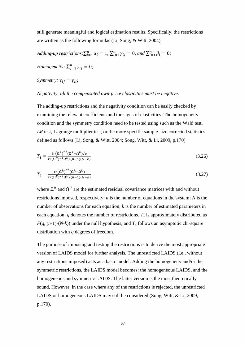
67
still generate meaningful and logical estimation results. Specifically, the restrictions
are written as the following formulas (Li, Song, & Witt, 2004)
Adding-up restrictions:∑ 𝛼𝑖𝑛𝑖=1 = 1, ∑ 𝛾𝑖𝑗
𝑛𝑖=1 = 0, and ∑ 𝛽𝑖
𝑛𝑖=1 = 0;
Homogeneity: ∑ 𝛾𝑖𝑗𝑛𝑗=1 = 0;
Symmetry: 𝛾𝑖𝑗 = 𝛾𝑗𝑖;
Negativity: all the compensated own-price elasticities must be negative.
The adding-up restrictions and the negativity condition can be easily checked by
examining the relevant coefficients and the signs of elasticities. The homogeneity
condition and the symmetry condition need to be tested using such as the Wald test,
LR test, Lagrange multiplier test, or the more specific sample-size corrected statistics
defined as follows (Li, Song, & Witt, 2004; Song, Witt, & Li, 2009, p.170)
𝑇1 =𝑡𝑟(Ω𝑅)
−1(Ω𝑅−Ω𝑈) 𝑞⁄
𝑡𝑟(Ω𝑅)−1Ω𝑈 (𝑛−1)(𝑁−𝑘)⁄ (3.26)
𝑇2 =𝑡𝑟(Ω𝑅)
−1(Ω𝑅−Ω𝑈)
𝑡𝑟(Ω𝑅)−1Ω𝑈 (𝑛−1)(𝑁−𝑘)⁄ (3.27)
where Ω𝑅 and Ω𝑈 are the estimated residual covariance matrices with and without
restrictions imposed, respectively; n is the number of equations in the system; N is the
number of observations for each equation; k is the number of estimated parameters in
each equation; q denotes the number of restrictions. T1 is approximately distributed as
F(q, (n-1)·(N-k)) under the null hypothesis, and T2 follows an asymptotic chi-square
distribution with q degrees of freedom.
The purpose of imposing and testing the restrictions is to derive the most appropriate
version of LAIDS model for further analysis. The unrestricted LAIDS (i.e., without
any restrictions imposed) acts as a basic model. Adding the homogeneity and/or the
symmetric restrictions, the LAIDS model becomes: the homogeneous LAIDS, and the
homogeneous and symmetric LAIDS. The latter version is the most theoretically
sound. However, in the case where any of the restrictions is rejected, the unrestricted
LAIDS or homogeneous LAIDS may still be considered (Song, Witt, & Li, 2009,
p.170).

68
From the estimated LAIDS model, the demand elasticities that have standard
interpretations can be calculated as follows (Song, Witt, & Li, 2009, pp.171-172).
Expenditure elasticity: it measures the sensitivity of demand for product/destination i
in response to changes in expenditure
휀𝑖𝑥 = 1 +𝛽𝑖
𝑤𝑖 (3.28)
Uncompensated price elasticities: they measure how a change in the price of one
product affects the demand for this product and for other products, with the total
expenditure and other prices held constant
휀𝑖𝑖 =𝜆𝑖𝑖
𝑤𝑖− 𝛽𝑖 − 1 (3.29)
and 휀𝑖𝑗 =𝜆𝑖𝑗
𝑤𝑖− 𝛽𝑖
𝑤𝑗
𝑤𝑖 (3.30)
Compensated price elasticities: they measure the price effects on the demand
assuming the real expenditure 𝑥 𝑃∗⁄ is constant
휀𝑖𝑖∗ =
𝛾𝑖𝑖
𝑤𝑖+ 𝑤𝑖 − 1 (3.31)
and 휀𝑖𝑗∗ =
𝛾𝑖𝑗
𝑤𝑖+ 𝑤𝑗 (3.32)
Applications
Although the AIDS model was introduced to tourism demand studies in as early as the
1980s, it has not attracted much attention until late 1990s (Li, Song, & Witt, 2005;
Sinclair, Black, & Sugiyarto, 2003). Built on strong economic underpinnings, the
AIDS model is often applied to model a specific stage of the budgeting process.
Many of the studies using AIDS model focus on the relatively early stage of
budgeting, where the tourists face with the allocations of expenditure within a group
of destinations. For example, De Mello, Pack, and Sinclair (2002) use a static AIDS
model to examine the UK demand for three neighbouring destinations, namely
France, Spain and Portugal. Similar approach is taken by Divisekera (2003), who, in
an attempt to generate a broad picture of international tourism, applies four individual
systems to model the tourism demand for Australia and selected international

69
destinations by residents from the UK, the USA, New Zealand and Japan. Dynamic
AIDS model, such as EC-LAIDS, gained popularity from mid-2000s. Examples are
Cortés-Jiménez, Durbarry, and Pulina (2009), Durbarry and Sinclair (2003), and Li,
Song, and Witt (2004), which model the outbound demand from Italy, France and the
UK, respectively.
Since the tourists are assumed to allocate their budget over a specified set of
destinations, tourism demand for the destinations in the system exhibits certain level
of interdependence. Specifically, the cross-price elasticities can denote whether
destinations are substitutes (positive elasticities) or complements (negative
elasticities). As remarked by Sinclair, Blake, and Sugiyarto (2003), the cross-price
elasticities are useful in indicating the degree of competitiveness or complementary
between different destinations. Studies that exploited the AIDS model’s capability of
gauging destination competitiveness are found sporadically after mid-2000s, such as
Li, Song, Cao, and Wu (2013), Mangion, Cooper, Cortés-Jimenez, and Durbarry
(2012), and Mangion, Durbarry, and Sinclair (2005).
Apart from modelling the allocations of budget over different destinations, the AIDS
model can also be used to analyse tourists’ consumptions of a range of products in a
particular destination, which correspond to a later stage of budgeting process. Tourism
expenditures are usually classified into five broad categories, namely,
accommodation, sightseeing/entertainment, food & beverage, shopping, and transport.
The AIDS model is used to reveal tourists’ sensitivities towards prices. Studies
emerged in the more recent literature include Wu, Li, and Song (2011), which specify
eight demand systems for eight major source markets to Hong Kong and compared
the elasticities of tourists from different markets. Other examples are Divisekera
(2009), Divisekera (2010b), and Wu, Li, and Song (2012).
Limitations
Although AIDS model is recognised for its rigorous economic underpinning and is
believed to generate more accurate estimates (especially regarding demand
elasticities), it faces criticism for not being able to account for endogeneity between
variables (Sinclair, Blake, & Sugiyarto, 2003). In an AIDS model, the dependent
variable in each equation is the share of expenditure on a particular
destination/product, whereas the explanatory variables are the price of each

70
destination/product and tourist’s total budget. Although interdependence between the
expenditures on different destinations/products is allowed, in the sense that a price
change in one destination/product will result in a change in the demand for that
particular destination/product as well as that for other destinations/products in the
same system, provided there exist substitution or complement relationships between
destinations/products. However, as with the single-equation models, the AIDS model
only allows for a one-way causal relationship running from prices and total budget to
expenditure share. The underlying assumption for the explanatory variables is still
that they are exogenous to the system. Such issues, as suggested by Sinclair, Blake,
and Sugiyarto (2003), can be resolved by using the VAR model to test if the AIDS
specification is appropriate, in that if both models yielded similar results, then with
confidence the AIDS model is not spurious.
Another issue with AIDS model is the over-parameterisation problem, which arises
when more destinations/products are added into the system. This is similar to the
curse of dimensionality that plagues VAR model, although the explosion of
parameters in AIDS model is not as serious as that of VAR model. From the standard
static model Eq. (3.24), adding one more destination/product will result in an
additional equation, and an additional price term for that destination/product in each
equation for other destinations/products in the same system. For example, if the
number of destinations/products increases from n to n+1, the additional parameters to
be estimated are 𝛼𝑛+1, 𝛽𝑛+1, 𝜆𝑛+1 and 𝛾𝑛+1,𝑗(𝑗 = 1, 2, … , 𝑛) in the (n+1)th equation,
and 𝛾𝑖,𝑛+1(𝑖 = 1, 2, … , 𝑛) in the other equations (the 1th to nth equation). Such an
increase of parameters can exhaust the degrees of freedom easily, given that the
observations (especially tourist expenditure data) typically cover a short time span.
Besides, an implication of the over-parameterisation is that the restriction tests are
more likely to be rejected, since the pattern of consumption (or the tourists’
behaviour) may not strictly follow the axioms of consumer choice if there are too
many destinations/products in question. Hampered by the over-parameterisation
problem, the AIDS model is only suitable for modelling a small demand system, just
as the VAR model.
A further limitation concerning the AIDS model is its relatively rigid specification.
Due to its rigorous economic underpinning, the choice of explanatory variables has

71
been well reasoned. As a result, the regressors in the model are constructed
exclusively from price variables and total budget variable, together with deterministic
terms such as intercepts, trend and/or dummies. Hence, as mentioned, although the
AIDS model allows for interdependence between destinations/products, such relations
can only be interpreted as results of the substitution effect and income effect
associated with price changes. Consequently, the connotation of ‘interdependencies’
under the AIDS framework is narrowly defined, leaving out the aspects such as the
feedback impact of tourism demand on local economy and the spillover effect on
foreign economies. It is also impossible to include new explanatory variables, apart
from the price and budget variables, since it would be deemed as lack of justification
under the neoclassical consumer theoretical framework, where the AIDS model draws
its theoretical grounding. In a word, the rigid specification of AIDS model limits the
scope of implications that can be drawn.
3.2.2.3 Panel Data Analysis
The Model
The panel data analysis is an advanced modelling approach which can be seen as an
extension of the single-equation models, and is able to accommodate the cross-
sectional dimension of data. Briefly speaking, there are three types of data structure.
The most often used in tourism demand modelling is time series data, as noted at the
beginning of Section 3.2.1. Time series data are continuous observations of variables
for a particular entity over a period of time (for example, a series of the UK’s GDP
figures from 2001 to 2013). The concern of using time series data is often about the
intrinsic characteristics of the entity’s evolution, or its dynamics. Another type of
structure is cross-sectional data, which are observations of variables for different
entities at a particular point of time (for example, a set of GDP figures of each of the
European Union member states in 2013). The concern of using cross-sectional data is
usually about the difference between the entities. A combination of the temporal
dimension and the cross-sectional dimension of data results in the third type of data
structure, i.e., the panel data (for example, a panel of GDP figures of each of the
European Union member states from 2001 to 2013).
Apparently, one of the advantages of panel data analysis is its relatively large number
of observations and the consequent increase in degrees of freedom (Song, Witt, & Li,
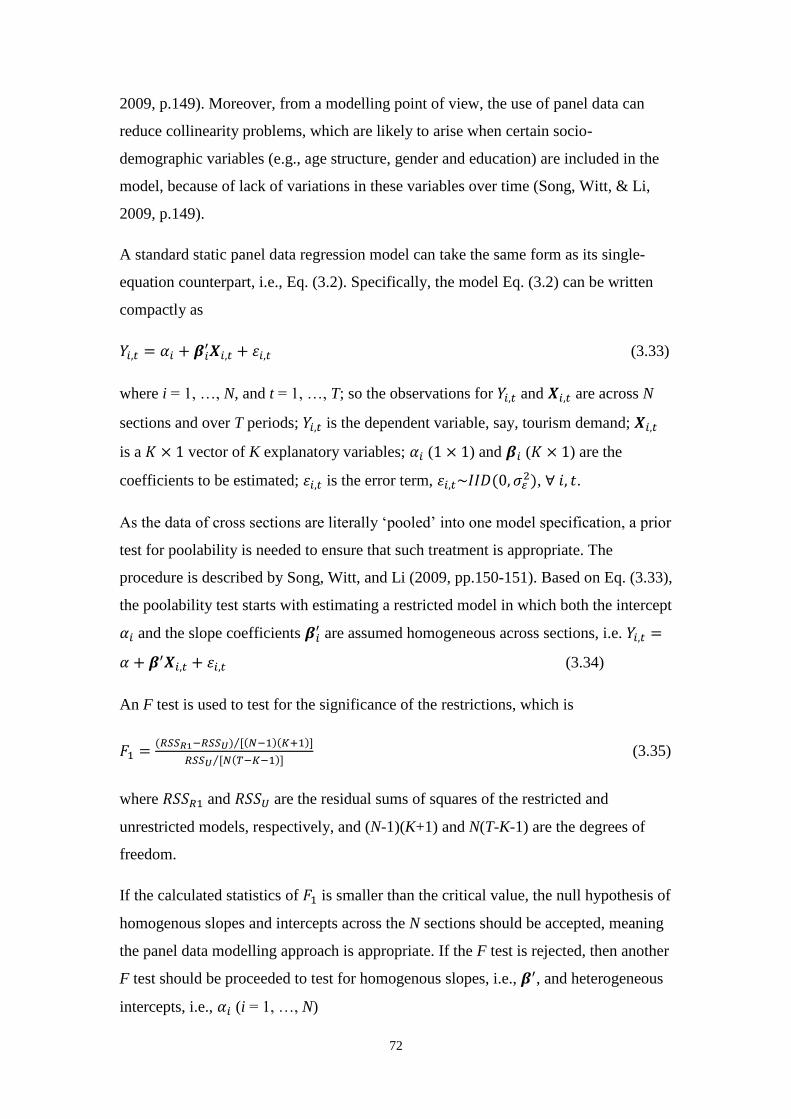
72
2009, p.149). Moreover, from a modelling point of view, the use of panel data can
reduce collinearity problems, which are likely to arise when certain socio-
demographic variables (e.g., age structure, gender and education) are included in the
model, because of lack of variations in these variables over time (Song, Witt, & Li,
2009, p.149).
A standard static panel data regression model can take the same form as its single-
equation counterpart, i.e., Eq. (3.2). Specifically, the model Eq. (3.2) can be written
compactly as
𝑌𝑖,𝑡 = 𝛼𝑖 + 𝜷𝑖′𝑿𝑖,𝑡 + 휀𝑖,𝑡 (3.33)
where i = 1, …, N, and t = 1, …, T; so the observations for 𝑌𝑖,𝑡 and 𝑿𝑖,𝑡 are across N
sections and over T periods; 𝑌𝑖,𝑡 is the dependent variable, say, tourism demand; 𝑿𝑖,𝑡
is a 𝐾 × 1 vector of K explanatory variables; 𝛼𝑖 (1 × 1) and 𝜷𝑖 (𝐾 × 1) are the
coefficients to be estimated; 휀𝑖,𝑡 is the error term, 휀𝑖,𝑡~𝐼𝐼𝐷(0, 𝜎𝜀2), ∀𝑖, 𝑡.
As the data of cross sections are literally ‘pooled’ into one model specification, a prior
test for poolability is needed to ensure that such treatment is appropriate. The
procedure is described by Song, Witt, and Li (2009, pp.150-151). Based on Eq. (3.33),
the poolability test starts with estimating a restricted model in which both the intercept
𝛼𝑖 and the slope coefficients 𝜷𝑖′ are assumed homogeneous across sections, i.e. 𝑌𝑖,𝑡 =
𝛼 + 𝜷′𝑿𝑖,𝑡 + 휀𝑖,𝑡 (3.34)
An F test is used to test for the significance of the restrictions, which is
𝐹1 =(𝑅𝑆𝑆𝑅1−𝑅𝑆𝑆𝑈) [(𝑁−1)(𝐾+1)]⁄
𝑅𝑆𝑆𝑈 [𝑁(𝑇−𝐾−1)]⁄ (3.35)
where 𝑅𝑆𝑆𝑅1 and 𝑅𝑆𝑆𝑈 are the residual sums of squares of the restricted and
unrestricted models, respectively, and (N-1)(K+1) and N(T-K-1) are the degrees of
freedom.
If the calculated statistics of 𝐹1 is smaller than the critical value, the null hypothesis of
homogenous slopes and intercepts across the N sections should be accepted, meaning
the panel data modelling approach is appropriate. If the F test is rejected, then another
F test should be proceeded to test for homogenous slopes, i.e., 𝜷′, and heterogeneous
intercepts, i.e., 𝛼𝑖 (i = 1, …, N)

73
𝐹2 =(𝑅𝑆𝑆𝑅2−𝑅𝑆𝑆𝑈) [(𝑁−1)𝐾]⁄
𝑅𝑆𝑆𝑈 [𝑁(𝑇−𝐾−1)]⁄ (3.36)
where 𝑅𝑆𝑆𝑅2 is the residual sum of squares for the restricted model where the
intercepts are allowed to vary across sections but the slope coefficients are equal.
If the calculated value of 𝐹2 is smaller than the critical value, the null hypothesis of
homogeneous slopes 𝜷 and heterogeneous intercepts 𝛼𝑖 will be accepted. In that case,
the use of panel data for modelling is appropriate.
Further to the 𝐹2 test, it is possible to test the null hypothesis of homogeneous
intercepts conditional on homogeneous slopes by a third F test, which is
𝐹3 =(𝑅𝑆𝑆𝑅1−𝑅𝑆𝑆𝑅2) (𝑁−1)⁄
𝑅𝑆𝑆𝑅2 (𝑁𝑇−𝑁−𝐾)⁄ (3.37)
If the intercept term, 𝛼𝑖, is assumed to be heterogeneous (according to the results of
the F tests), appropriate dummy variables will be needed to account for the section-
specific difference. There are two models that can be considered, which are the fixed
effects (FE) model and the random effects (RE) model.
Specifically, the error term in Eq. (3.33) can be re-specified as
휀𝑖,𝑡 = 𝑢𝑖 + 𝑒𝑖,𝑡 (3.38)
where 𝑢𝑖 denotes the unobservable section-specific effects and 𝑒𝑖,𝑡 is the usual
disturbance term, which varies across sections and period (Song, Witt, & Li, 2009,
p.152).
The difference between the fixed effects (FE) model and the random effects (RE)
model lies in the assumptions made about 𝑢𝑖. The FE model assumes that 𝑢𝑖 is
correlated with explanatory variables 𝑿𝑖,𝑡, whereas the RE model assumes that 𝑢𝑖 is
uncorrelated with 𝑿𝑖,𝑡. A priori considerations suggest that the FE model is one from
which inferences can be made conditional on the observed sample. Hence, if the focus
is on the sample itself, the FE model is appropriate. But if the concern is about
drawing inferences with regard to the population based on the sample, then the RE
model is more appropriate (Song, Witt, & Li, 2009, p.152).
74
As with the single-equation approach, dynamics of the data can also be incorporated
into panel data analysis through inclusion of lagged dependent variable, which is often
interpreted as a measure of habit persistence and/or word-of-mouth effect of tourism
demand1 (Garín-Munoz, 2006; Naude & Saayman, 2005; Seetaram, 2010). Following
Eq. (3.34) and Eq. (3.38), a dynamic panel data regression model can be written as
𝑌𝑖,𝑡 = 𝛼 + 𝛾𝑌𝑖,𝑡−1 + 𝜷′𝑿𝑖,𝑡 + 𝑢𝑖 + 𝑒𝑖,𝑡 (3.39)
where 𝛾 is the coefficient to be estimated, in addition to 𝜷.
Model Estimation
The procedure of panel data regression is very similar to that of the single-equation
models. It starts with the tests for cointegrating relation, which involve both the unit
root tests and the cointegration tests. As noted by Seetanah, Durbarry, and Ragodoo
(2010), the commonly used unit root tests, such as the augmented Dickey-Fuller
(ADF) and Phillips-Perron (PP), have low power in distinguishing the unit root null
from the stationary alternatives in the context of panel data. Special panel unit root
tests have thus been devised.
The development of panel unit root tests basically centres on two issues:
heterogeneity and cross-sectional dependencies (Hurlin & Mignon, 2007).
Specifically, the panel unit root tests proposed in early literature assumed cross-
sectional independence, which means there is no potential correlation across residuals
of panel units. These tests are generally termed as the first generation panel unit root
tests, for instance, Levin, Lin, and Chu (2002), Im, Pesaran, and Shin (2003), Maddala
and Wu (1999), Choi (2001) and Hadri (2000). The first generation tests are divided
with regard to whether the panel is homogeneous or heterogeneous across sections. In
other words, the question is if the same model can be used to test the unit root
hypothesis on various individual sections. A positive answer means that the panel is
homogeneous. For instance, the Levin, Lin, and Chu (LLC) and the Hadri tests
assume that there is a common unit root process, so the autoregressive parameter in
the test model is identical across sections. On the contrary, if each section is
1 As cited in Section 3.2.1.2, Morley (2009) pointed out a few justifications for including lagged terms
of variables in a model. Hence, the lagged terms have rich underpinning and the interpretation should
not be limited to habit persistence only.

75
characterised by its unique dynamics, the panel is then heterogeneous and the unit
root tests have to account for the heterogeneity. The Im, Pesaran, and Shin (IPS),
Fisher-type ADF and PP tests (Maddala & Wu, 1999; Choi, 2001) allow for
individual unit root processes, so the autoregressive parameter may vary across
sections. The tests are characterised by the combining of individual unit root tests to
derive a panel-specific result. In the tourism demand studies that adopted dynamic
panel data analysis, the latter category of panel unit root tests, which take the
heterogeneity into consideration, is often chosen (e.g., Ledesma-Rodriguez, Navarro-
Ibanez, & Perez-Rodriguez, 2001; Seetanah, Durbarry, & Ragodoo, 2010; Seetaram,
2010).
As opposed to the first generation panel unit root tests, the second generation tests
relax the cross-sectional independence assumption. It is argued that the cross-sectional
independency hypothesis is rather restrictive and somewhat unrealistic in the majority
of macroeconomic applications where co-movements of economies are often observed
(Hurlin & Mignon, 2007). In attempting to exploit the co-movements across sections
in order to define new test statistics, two main approaches have been followed. The
first one specifies the cross-sectional dependencies as a common factor model, for
example, the Bai and Ng (2004), Phillips and Sul (2003), Moon and Perron (2004),
Choi (2006), and Pesaran (2007) tests. The second approach imposes few or none
restrictions on the covariance matrix of residuals, for example, Chang (2002).
After the panel unit root tests, panel cointegration tests are performed to confirm the
long-run relationship among variables. Commonly used methods are residual-based
panel cointegration tests such as those proposed by Kao (1999) and Pedroni (1999,
2004). Examples using these methods are Falk (2010), Seetanah, Durbarry, and
Ragodoo (2010), and Seetaram (2010). The Pedroni’s tests rely on four panel statistics
(equivalent to the unit root statistics against homogeneous alternatives) and three
group mean panel statistics (analogous to the panel unit root tests against
heterogeneous alternatives) to test the null hypothesis of no cointegration against the
alternative of cointegration (Breitung & Pesaran, 2005; Seetanah, Durbarry, &
Ragodoo, 2010).
Once the panel cointegration tests have been conducted, an appropriate estimator has
to be chosen to estimate the panel data regression model. As widely acknowledged,

76
the traditional ordinary linear squares (OLS) estimator will generate biased and
inconsistent estimates when applied to a dynamic panel data model specification
(Ledesma-Rodriguez, Navarro-Ibanez, & Perez-Rodriguez, 2001; Naude & Saayman,
2005; Seetaram, 2010). Another standard estimator for panel data, least squares
dummy variable (LSDV), is also problematic in the presence of lagged dependent
variables (Deng & Athanasopoulos, 2011). The problem occurs because of the
correlation between the lagged dependent variable and the error term of the regression
model; that is the regressors are not exogenous. It is only when there is a large number
of observations in the temporal dimension that the problem of biased and inconsistent
estimates will be alleviated (Deng & Athanasopoulos, 2011; Garín-Muñoz &
Montero-Martín, 2007; Seetaram, 2010).
To properly estimate the dynamic panel, early literature (e.g., Ledesma-Rodriguez,
Navarro-Ibanez, & Perez-Rodriguez, 2001) used the instrument variable (IV) type of
estimators, such as the two-stage least squares (TSLS) and the three-stage least
squares (3SLS), where two period lagged values of the dependent variable are used as
the IV. However, this approach leads to consistent but not efficient estimates, because
it does not make use of all the variable moment conditions (Garín-Muñoz & Montero-
Martín, 2007). More efficient estimators have been developed under the generalised
method of moments (GMM) framework based on the studies by Arellano and Bond
(1991) and Arellano and Bover (1995), who used high order of lagged dependent
variables as IV, and this approach has become the most popular (Deng &
Athanasopoulos, 2011). Examples using the GMM type estimators include Balli,
Balli, and Cebeci (2013), Garín-Muñoz and Montero-Martín (2007), Khadaroo and
Seetanah (2008), Massidda and Etzo (2012), Naude and Saayman (2005), Rodríguez,
Martínez-Roget, and Pawlowska (2012). However, as noted by Seetaram (2010), if
the time span of the data is small, the bias persists even if the GMM estimator is
applied. It is argued that the corrected LSDV (CLSDV) estimator proposed by Kiviet
(1995) will be more efficient when T is small, although it is only applicable to
balanced panel data.
Applications
As introduced, panel data analysis can accommodate both the temporal and spatial (or
cross-sectional) dimensions of tourism demand data. Therefore, it is suitable for
77
models of which the data cover a shorter time span and have different cross sections.
Despite the advantages of panel data, their applications were rarely seen when Song
and Li (2008) conduct a thorough survey in the mid-2000s. It is until more recently
(the late-2000s) that this modelling approach has been more frequently exploited and
become a favoured choice for certain research topics.
A primary application is modelling tourism demand and measuring the
effects/elasticities of relevant determinants. This has appeared in studies majorly since
the early 2000s. For example, Ledesma-Rodriguez, Navarro-Ibanez, and Perez-
Rodriguez (2001) estimate both short-run and long-run elasticities of demand for
Tenerife tourism, based on a panel of arrival figures to thirteen source countries.
Other examples are Falk (2010), Garín-Muñoz and Montero-Martín (2007), Naude
and Saayman (2005), and Seetaram (2010). The ability of panel data to handle the
collinearity problems associated with the relatively time-invariant socio-demographic
data allows studies to include these variables and extend the scope of research (e.g.,
Nerg, Uusivuori, Mikkola, Neuvonen, & Sievanen, 2012).
One time-invariant factor that especially attracts researchers’ attention is distance. A
range of studies have been based on the gravity models to analyse tourism flows. The
idea of gravity models was originally derived by analogy with Newton’s gravitational
law. It states (in the tourism context) that the degree of interaction between two
geographic areas varies directly with the degrees of concentration of persons in two
areas and inversely with the distance separating them (Witt & Witt, 1995). The basic
form of gravity models is
𝑇𝑖𝑗 = 𝑎(𝑃𝑖𝑏1𝑃𝑗
𝑏2 𝑑𝑖𝑗𝑏3⁄ ) (3.40)
where 𝑇𝑖𝑗 denotes the number of trips taking between node i and node j; Pi and Pj are
the population at node i and node j; dij is the distance between node i and node j; and
a, b1, b2 and b3 are constants.
When used in empirical studies, the model specifications often include explanatory
variables such as income, prices as well as other socio-economic factors, thus closely
resembling usual consumer theory-based demand function. Despite that the gravity
model was recognised to be well suited to studying international trade (Khadaroo &
Seetanah, 2008), its applications in tourism demand research were not widely

78
observed, nor was it surveyed systematically in review papers, except for Witt and
Witt (1995). Nevertheless, it emerges that gravity models have become an often
choice in recent literature using panel data, for example, Deng and Athanasopoulos
(2011), Eryigit, Kotil, and Eryigit (2010), Khadaroo and Seetanah (2008), Massidda
and Etzo (2012), and Seetanah, Durbarry, and Ragodoo (2010).
Limitations
The primary issue with panel data analysis is on the poolability assumption, which
needs to be tested before modelling exercise is carried out. As remarked by Song,
Witt, and Li (2009, p.149), ‘the choice of an appropriate model depends inter alia on
the degree of homogeneity of the intercept and slope coefficients and the extent to
which any individual cross-section affects are correlated with the explanatory
variables’. Although it is allowed that the intercepts to be heterogeneous by
employing the fixed effect or random effect models, the slope coefficients are
generally set to be identical in the setting of panel data analysis. An observation about
the studies since the early 2000s shows that, however, the poolability tests are
generally left out. The model specifications (e.g., fixed effect or random effect
models) are often determined on a priori basis. This will inevitably cause concerns
about the rigor underlying the models.
Based on the existing literature, it is found that another issue which limits the
applications of panel data analysis is exactly the one that troubles the models
introduced in previous sections – exogeneity. The specifications of panel data
regression models, i.e., Eq. (3.33) and Eq. (3.39), resemble those of the single-
equation models. Following Eq. (3.39), which considers the fixed effect or random
effect, several assumptions about the error terms 𝑒𝑖,𝑡 and the unobserved
heterogeneity terms 𝑢𝑖 are made. As summarised by Seetaram (2010), these state that
(i) the error terms are not correlated to one another over the sample period and across
sections; (ii) the unobserved heterogeneity is random; (iii) the unobserved
heterogeneity is uncorrelated within the sections and with the error terms; (iv) the
explanatory variables are strictly exogenous, i.e., not correlated with the error terms;
and (v) the unobserved heterogeneity may be correlated with predetermined variables.
Therefore, bidirectional causation is not allowed under the panel data setting.

79
Endogeneity among dependent and explanatory variables cannot be modelled under
the existing panel data analytical framework.
3.2.3 Other Econometric Model
Time Varying Parameters (TVP) Model
As raised in Section 3.2.1.3, the single-equation approach rigidly assumes that the
coefficients to be estimated are constant over the whole sample period. The
consequence is that the demand elasticities calculated accordingly will be constant as
well. It would be unrealistic to assume that people’s consumption behaviour remains
the same consistently, especially if tourism market and local economy have
undergone radical changes during the sample period.
One of the recurrent features of the econometric models has been predictive failure,
which is normally associated with model structure instability, i.e., the parameters of
the demand model vary over time (Song, Witt, & Li, 2009, p.138). There are
generally two reasons for structural instability. The first is that our knowledge about
the structure of model is limited. Hence, when a predictive failure occurs, new
information should be added to the knowledge base, which is used to produce a better
model that encompasses both the new and earlier information (Song, Witt, & Li,
2009, p.138). This leads to the use of recursive-OLS, which is to re-specify the model
every time a new observation from the sample is added. The second reason for
structural instability is that it is a reflection of underlying structural change in the data
generating process (DGP). This may be related to important social, political and
economic changes (Song, Witt, & Li, 2009, p.138). To account for the underlying
changes embedded in the data, time varying parameter (TVP) model has been
proposed and also applied to tourism demand studies.
The TVP model can be specified in the following state space form
𝑦𝑡 = 𝑥𝑡𝛼𝑡 + 휀𝑡 (3.41)
𝛼𝑡+1 = 𝑇𝑡𝛼𝑡 + 𝑅𝑡𝜂𝑡 (3.42)
where 𝑦𝑡 is the dependent variable; 𝑥𝑡 is a row vector of k explanatory variables; 𝛼𝑡 is
a column vector of k state variables known as the state vector; 𝑇𝑡 is a k × k matrix; 𝑅𝑡
is a k × g matrix; 휀𝑡 refers to the temporary disturbance, 휀𝑡~𝑁(0,𝐻𝑡); 𝜂𝑡 is g × 1

80
vector of permanent disturbance, 𝜂𝑡 ~𝑁(0, 𝑄𝑡); both 휀𝑡 and 𝜂𝑡 are Gaussian
disturbances, which are serially uncorrelated and independent of each other at all time
points (Li, Wong, Song, & Witt, 2006). Eq. (3.41) is called the system equation or
observation equation, while Eq. (3.42) is called the transition equation or state
equation (Li, Wong, Song, & Witt, 2006; Song, Witt, & Li, 2009, pp.142-143). The
equations can easily be extended to accommodate a vector of dependent variables, and
in that case, both𝑦𝑡 and 휀𝑡 become a vector accordingly.
The components of the matrix 𝑇𝑡 in Eq. (3.42) can equal unity. The transition equation
then becomes a random walk:
𝛼𝑡+1 = 𝛼𝑡 + 𝑅𝑡𝜂𝑡 (3.43)
In most of the economic applications, it is assumed that 𝛼𝑡 follows a random walk
process (Li, Wong, Song, & Witt, 2006). Other specifications of the transition
equation can be determined by experimentation. The criteria are the goodness of fit
and the predictive power of the model (Song, Witt, & Li, 2009, p.143). Once the
model (both the system equation and the transition equation) is formulated, it can be
estimated with the Kalman filter (KF), which is a recursive procedure for calculating
the optimal estimator of the state vector given all the information available at time t.
Despite the advantages of TVP model, its applications in tourism research is still
relatively limited. Song and Wong (2003) applied the model to examine the demand
for Hong Kong tourism from six major countries of origins. In their assessment of the
impacts of the global economic crisis and swine flu on the demand for UK tourism,
Page, Song, and Wu (2012) construct a TVP model to yield ex post forecasts of
demand under the no-impact and economic-impact scenario, and estimated the events’
impacts by comparing the two scenarios. It was justified by the fact that the external
shocks, such as economic crisis and global pandemic, would cause structural change
to tourists’ behaviour.
TVP model is also used in combination with other models, in order to achieve
superior performance. Li, Wong, Song, and Witt (2006) is the first study in the
context of tourism demand forecasting to apply the TVP-LRM and TVP-ECM to
modelling the demand for European destinations by UK residents. The models were
then compared with a number of fixed-parameter models, including naïve, ARIMA,

81
ADLM, VAR, ECM. It was found that the TVP-ECM consistently outperformed the
fixed-parameter econometric models and time series models. The combination of TVP
model and other models is not limited to single-equation models only. Li, Song, and
Witt (2006) develop the TVP-LAIDS models in both long-run (LR) form, i.e., TVP-
LR-LAIDS, and error correction (EC) form, i.e., TVP-EC-LAIDS. Based on the
figures of UK’s outbound tourists to Western Europe, both the TVP versions and their
fixed-parameter counterparts were estimated and compared. The results suggested that
the unrestricted TVP-LR-LAIDS and TVP-EC-LAIDS outperformed their fixed-
parameter counterparts in the overall evaluation of demand level forecasts. Wu, Li,
and Song (2012) apply the TVP-EC-LAIDS model to analyse the consumption
behaviour of tourists to Hong Kong.
3.3 Time Series Models
In contrast to the econometric models, time series models require standalone series of
the variable only. For example, to model tourism demand, a series of demand figures
(e.g., tourist arrivals or tourism expenditure) covering a certain time span will be the
only input. Explanatory variables can be entirely omitted in the model. Particular
attention is thus paid to exploring the historic trends and patterns (such as cycle and
seasonality) of the series and to predicting the future values of the series based on the
properties identified1 (Song & Li, 2008), rather than pursuing the underlying causal
relations. As a result, the use of time series models is closely associated with
forecasting exercise, and the models under this category often become contenders for
forecasting competition.
As less inputs are required in time series models, the data collection process can thus
be greatly shortened, provided sufficient number of observations is available.
Although it is desirable to obtain high frequency data2 (e.g., monthly, weekly, and
daily) as the number of observations will be larger, the associated sophistication of
patterns will increase the difficulty of modelling.
A critical limitation of time series models, in comparison with the econometric
models, is that no causal relationship can be modelled. Hence, it is not possible to
1 It is assumed that past trends and/or features of a time series will repeat in the future. Hence, the
model that identifies the intrinsic properties of historic data can be used for forecasting exercise. 2 Apparently, ‘high frequency’ in the context of tourism demand modelling is not comparable to that
used in the field of finance, where data be generated every day, hour, minute, or second.
82
incorporate economic theory and/or tourism theory into the model. It will also be
difficult to attach a practical meaning to the parameters estimated, except that they
reveal certain intrinsic attributes of the data. Nevertheless, time series models are still
popular with tourism researchers, due to its relatively easy implementation process
and potential use as benchmarks for forecast competition. Given that the current
research will be conducted under the framework of econometric models, time series
models are less relevant. Hence the following review will be conducted in a succinct
manner.
3.3.1 Autoregressive Integrated Moving Average (ARIMA) Models
Time series models have been widely used for tourism demand modelling. Among
others, the autoregressive integrated moving average (ARIMA) model, which was
proposed by Box and Jenkins in the 1970s, is the most popular (Goh & Law, 2011;
Song & Li, 2008). This is because, as remarked by Lim and McAleer (2002), it can
handle any stationary or non-stationary time series, both with and without seasonal
elements.
The ARIMA model accommodates both autoregressive (AR) process and moving
average (MA) process. Briefly speaking, the AR process specifies that the dependent
variable depends linearly on its own past values, whereas the MA process suggests
that the current value of dependent variable is a linear combination of current and
previous white noise error terms. A general representation of an ARIMA (p, q, d)
model is
(1 − ∑ 𝜙𝑖𝐿𝑖𝑝
𝑖=1 )(1 − 𝐿)𝑑𝑋𝑡 = (1 + ∑ 𝜃𝑖𝐿𝑖𝑞
𝑖=1 )휀𝑡 (3.44)
where L is the lag operator; 𝑋𝑡 is the variable under study; 휀𝑡 is the error term; 𝜙𝑖 (i =
1, 2, …, p) are the parameters of the AR part of the model; 𝜃𝑖 (i = 1, 2, …, p) are the
parameters of the MA part of the model; correspondently, p is the order of the AR
process and q the MA process; i is the order of integration of the time series; d
denotes the order of differencing applied to the series. If d=0, the model is equivalent
to an ARMA model.
In addition to the ‘simple’ ARIMA outlined above, variations and extensions of the
ARIMA model have also been introduced. They are sometimes categorised as
‘ARMA-based’ models (Chu, 2009) or ‘ARIMA-based’ models (Tsui, Balli, Gilbey,
83
& Gow, 2014). One of the most often seen variations is the seasonal ARIMA
(SARIMA) model, which is applied when seasonal data are used and seasonal effects
are suspected. Seasonal differencing is performed up to order D. Seasonal parameters
of the AR part and the MA part are incorporated into the model. Another variation
that regularly features in the recent tourism demand literature is the fractional ARIMA
(ARFIMA) model. It is a generalisation of the ARIMA that incorporates long-range
dependence. In an ARFIMA model, the differencing parameter d is allowed to be a
non-integer, denoting the fractional order of integration (Chu, 2009). A further
variation of ARIMA model is the ARAR model. The idea is that a time series is
transformed from a long-memory AR filter to a short-memory filter. It explicitly
questions the practice of differencing to achieve stationary and has an advantage of
utilizing information contained in the data, normally lost when differencing (Chu,
2009).
Given the range of variations, it is seldom that an ARIMA model will be employed as
a standalone model. Comparison is often involved between alternative models. In
modelling and forecasting the international tourism demand for Australia, Lim and
McAleer (2002) compared the forecast performance of both ARIMA and SARIMA
model. Chu (2009) compared the forecast performance of SARIMA, ARAR and
ARFIMA model, based on the international arrival figures to nine major destination
countries in Asia-Pacific region. It is found that the ARFIMA model in general
outperformed the other two. Shen, Li, and Song (2009) extend the scope of
comparison, to include econometric models (e.g., ECM) as alternatives. The results
showed that no single model could consistently outperform the others on all
occasions, though. Some other examples are Chu (1998), Chu (2008a), Chu (2008b),
Goh and Law (2002), and Nowman and Van Dellen (2012).
3.3.2 Generalised Autoregressive Conditional Heteroskedasticity (GARCH)
Models
Volatility models have been very popular with empirical research in finance and
econometrics since the early 1990s (Coshall, 2009). The models are based on the
influential papers by Engle (1982) and Bollerslev (1986). At the root of volatility
modelling is the distinction between conditional (stochastic) and unconditional
(constant) errors. The models contain a ‘mean equation’, which is commonly a
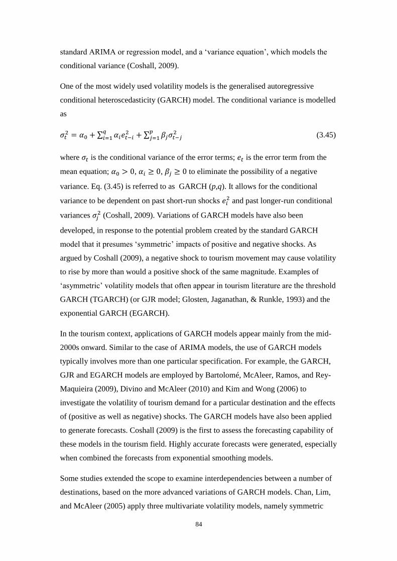
84
standard ARIMA or regression model, and a ‘variance equation’, which models the
conditional variance (Coshall, 2009).
One of the most widely used volatility models is the generalised autoregressive
conditional heteroscedasticity (GARCH) model. The conditional variance is modelled
as
𝜎𝑡2 = 𝛼0 + ∑ 𝛼𝑖𝑒𝑡−𝑖
2𝑞𝑖=1 + ∑ 𝛽𝑗𝜎𝑡−𝑗
2𝑝𝑗=1 (3.45)
where 𝜎𝑡 is the conditional variance of the error terms; 𝑒𝑡 is the error term from the
mean equation; 𝛼0 > 0, 𝛼𝑖 ≥ 0, 𝛽𝑗 ≥ 0 to eliminate the possibility of a negative
variance. Eq. (3.45) is referred to as GARCH (p,q). It allows for the conditional
variance to be dependent on past short-run shocks 𝑒𝑖2 and past longer-run conditional
variances 𝜎𝑗2 (Coshall, 2009). Variations of GARCH models have also been
developed, in response to the potential problem created by the standard GARCH
model that it presumes ‘symmetric’ impacts of positive and negative shocks. As
argued by Coshall (2009), a negative shock to tourism movement may cause volatility
to rise by more than would a positive shock of the same magnitude. Examples of
‘asymmetric’ volatility models that often appear in tourism literature are the threshold
GARCH (TGARCH) (or GJR model; Glosten, Jaganathan, & Runkle, 1993) and the
exponential GARCH (EGARCH).
In the tourism context, applications of GARCH models appear mainly from the mid-
2000s onward. Similar to the case of ARIMA models, the use of GARCH models
typically involves more than one particular specification. For example, the GARCH,
GJR and EGARCH models are employed by Bartolomé, McAleer, Ramos, and Rey-
Maquieira (2009), Divino and McAleer (2010) and Kim and Wong (2006) to
investigate the volatility of tourism demand for a particular destination and the effects
of (positive as well as negative) shocks. The GARCH models have also been applied
to generate forecasts. Coshall (2009) is the first to assess the forecasting capability of
these models in the tourism field. Highly accurate forecasts were generated, especially
when combined the forecasts from exponential smoothing models.
Some studies extended the scope to examine interdependencies between a number of
destinations, based on the more advanced variations of GARCH models. Chan, Lim,
and McAleer (2005) apply three multivariate volatility models, namely symmetric

85
CCC-MGARCH, symmetric vector ARMA-GARCH and asymmetric vector ARMA-
AGARCH model, to investigate the volatility of demand for Australian tourism by
four leading source markets. Presence of cross-country dependence was detected
among the four markets, in the sense that the conditional variance of a particular
country was affected by previous short- and long-run shocks from other countries.
Other similar applications include Chang, Khamkaew, Tansuchat, and McAleer
(2011) and Seo, Park, and Yu (2009).
It is, however, argued that the interdependencies detected (or defined) under the
GARCH model framework are rather narrow, because essentially only the spillover
effect of shocks to tourism demand is modelled. As with the other time series models,
causal relationships between tourism demand and economic factors are missed in the
GARCH model. Hence, the effect of shocks to the underlying economic variables
cannot be studied using the GARCH model, let alone the feedback impact of tourism
demand on the economic factors.
Another criticism for the GARCH models comes from Morley (2012), who
challenged that ‘it is indeed difficult to conceive of a theoretical justification for
models like ARCH in tourism’. No reason was provided why tourism time series
would be likely to have volatility issues similar to financial time series, or why these
specific models would be relevant to tourism data. In its absence, researchers simply
announced that the models will be used, as if the technique’s existence were sufficient
justification and rationale in itself (Morley, 2012).
3.3.3 Other Time Series Models
The Naïve Model
The naïve model represents a rather simple way of understanding historic trend. It
assumes data evolve based on certain static growth rate. Hence, future is only a simple
repeat of history. The model is often used for forecasting purposes and acts as a
benchmark against more sophisticated models.
Generally there are two naïve models used in the tourism demand literature. The naïve
1 model is a no-change model, which states that the future value will be equal to the
latest available value, i.e., �̂�𝑡 = 𝑦𝑡−1. In the case where seasonal data are used, the

86
naïve 1 model can become �̂�𝑡 = 𝑦𝑡−4. So the forecast value for a certain quarter is
exactly the value of the corresponding quarter in the previous year.
The naïve 2 model is a constant growth rate model, which suggests that the value of a
variable will grow at constant rate, hence the future values can be deduced based on
the growth rate, i.e., �̂�𝑡 = 𝑦𝑡−1[1 + (𝑦𝑡−1 − 𝑦𝑡−2) 𝑦𝑡−2⁄ ]. Again, if seasonal data are
used, the model becomes �̂�𝑡 = 𝑦𝑡−4[1 + (𝑦𝑡−4 − 𝑦𝑡−8) 𝑦𝑡−8⁄ ].
The naïve models widely feature in demand forecasting studies. They often offer
baseline forecasts for comparison (e.g., Chu, 2008; Shen, Li, & Song, 2009); or they
constitute one of the components of combined forecasts (e.g., Cang, 2011; Shen, Li, &
Song, 2008; and Shen, Li, & Song, 2011).
Exponential Smoothing (ES) Model
Exponential smoothing (ES) is a commonly used technique to produce smoothed data
for presentation, or to make forecasts. It essentially follows the moving average
method. Forecasts of future values are based on the weighted averages of the past
values, with the highest weight assigned to the most recent observation and the
weights decreasing exponentially for more distant observations (Lim & McAleer,
2001b).
In its simple (or single) form of the ES model, the forecast in period t is based on
weighting the observation in period t by a smoothing factor 𝛼, and the most recent
forecast by (1 − 𝛼). The single exponential smoothing method is appropriate only for
stationary and non-seasonal time series with no structural change. More advanced
algorithms, such as double exponential smoothing, Holt’s method and Holt-Winter’s
method, have been developed and applied in the tourism literature. The forecast
performance of the various exponential smoothing methods has often been discussed.
For example, based on the quarterly figures of arrivals to Australia over the last 25
years of the 20th century, Lim and McAleer (2001b) find that the Holt-Winters
addictive and multiplicative seasonal models outperformed the single, double, and the
Holt-Winters non-seasonal ES models in forecasting. Cho (2003) compares the
Winters multiplicative ES model with an ARIMA and an artificial neural networks
(ANN) model, in order to predict the travel demand for Hong Kong. The results from
the ANN model were more favourable, though. However, using data on tourism
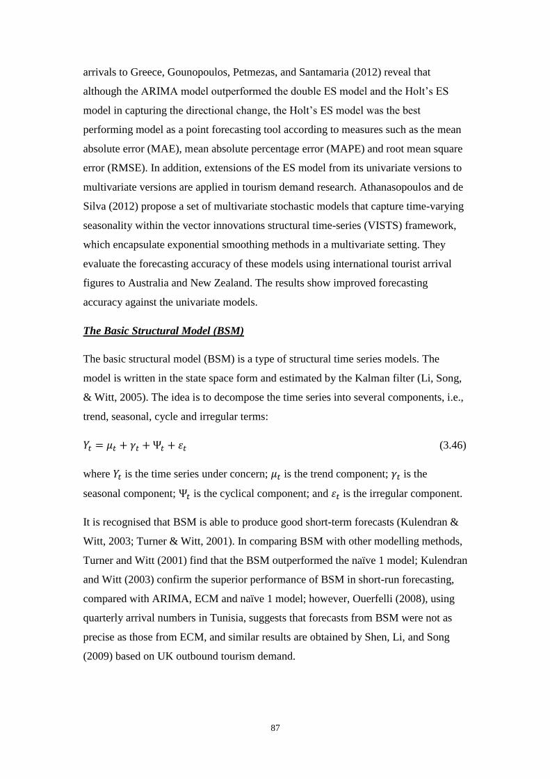
87
arrivals to Greece, Gounopoulos, Petmezas, and Santamaria (2012) reveal that
although the ARIMA model outperformed the double ES model and the Holt’s ES
model in capturing the directional change, the Holt’s ES model was the best
performing model as a point forecasting tool according to measures such as the mean
absolute error (MAE), mean absolute percentage error (MAPE) and root mean square
error (RMSE). In addition, extensions of the ES model from its univariate versions to
multivariate versions are applied in tourism demand research. Athanasopoulos and de
Silva (2012) propose a set of multivariate stochastic models that capture time-varying
seasonality within the vector innovations structural time-series (VISTS) framework,
which encapsulate exponential smoothing methods in a multivariate setting. They
evaluate the forecasting accuracy of these models using international tourist arrival
figures to Australia and New Zealand. The results show improved forecasting
accuracy against the univariate models.
The Basic Structural Model (BSM)
The basic structural model (BSM) is a type of structural time series models. The
model is written in the state space form and estimated by the Kalman filter (Li, Song,
& Witt, 2005). The idea is to decompose the time series into several components, i.e.,
trend, seasonal, cycle and irregular terms:
𝑌𝑡 = 𝜇𝑡 + 𝛾𝑡 +Ψ𝑡 + 휀𝑡 (3.46)
where 𝑌𝑡 is the time series under concern; 𝜇𝑡 is the trend component; 𝛾𝑡 is the
seasonal component; Ψ𝑡 is the cyclical component; and 휀𝑡 is the irregular component.
It is recognised that BSM is able to produce good short-term forecasts (Kulendran &
Witt, 2003; Turner & Witt, 2001). In comparing BSM with other modelling methods,
Turner and Witt (2001) find that the BSM outperformed the naïve 1 model; Kulendran
and Witt (2003) confirm the superior performance of BSM in short-run forecasting,
compared with ARIMA, ECM and naïve 1 model; however, Ouerfelli (2008), using
quarterly arrival numbers in Tunisia, suggests that forecasts from BSM were not as
precise as those from ECM, and similar results are obtained by Shen, Li, and Song
(2009) based on UK outbound tourism demand.

88
3.3.4 Time Series Models Augmented With Explanatory Variables
An emerging trend of tourism demand research has been the introduction of the
advanced time series techniques into the econometric (or causal) regression
framework (Li, Song, & Witt, 2005). By integrating both methods, the merits of
econometric models and time series models are combined. Two notable examples of
this category are the autoregressive integrated moving average model with
explanatory variables (ARIMAX) and the structural time series model (STSM).
ARIMAX Model
The AR(I)MAX model is an extension of the pure time series model AR(I)MA, by
including additional exogenous independent variables. Given the favourable
performance of time series in tourism demand forecasting, it has been recommended
that including causal variables in a time series formulation will improve the model. It
can also be taken that adding time series terms to a causal model is likely to yield
better performance (Morley, 2009).
The general ARIMAX model can be written as
(1 − ∑ 𝛼𝑖𝐿𝑖𝑝
𝑖=1 )(1 − 𝐿)𝑑𝑌𝑡 = ∑ 𝜷𝑖′𝐿𝑖𝑿𝑡
𝑟𝑖=0 + (1 + ∑ 𝛾𝑖𝐿
𝑖𝑞𝑖=1 )휀𝑡 (3.47)
where L is the lag operator; 𝑌𝑡 is the dependent variable; 𝑿𝑡 is a 𝑘 × 1 vector of
explanatory variables;휀𝑡 is the white noise error term; 𝛼𝑖 , 𝛽𝑖 and 𝛾𝑖 are the parameters
to be estimated; p, q and r are the lag length of the AR part, MA part and the
explanatory variables, respectively; d is the differencing parameter. It is advised that
the ARIMA model that doesn’t include explanatory variables needs to be identified
before constructing the ARIMAX model (Kuo, Chen, Tseng, Ju, & Huang, 2008).
Several applications of the AR(I)MAX model have emerged since the mid-2000s.
Akal (2004) specifies an ARMAX model to forecast Turkey’s tourism revenues
between 2002 and 2007. The number of international arrivals was used as an
explanatory variable for the tourism revenue figures, although it is questionable
whether such choice of explanatory variable is appropriate because essentially both
the arrival figures and the revenue figures are indicators of the same thing and they
are endogenous to each other. Other applications are, for example, Lim, Min, and
McAleer (2008), who model the effects of income on Japan’s outbound tourism

89
demand; Kuo, Chen, Tseng, Ju, and Huang (2008), who assess the impacts of SARS
and avian flu on the international tourism demand to Asia; Yang, Pan, and Song
(2013), who predict the hotel demand based on the web traffic volume of a destination
marketing organisation (DMO). Morley (2009) compares the ARIMAX model with a
range of dynamic tourism demand models such as ADLM, ECM, and found the
specification of ARIMAX was better than other dynamic models based on the adjust
R-squared.
Structural Time Series Model (STSM)
Similar to the AR(I)MAX model, explanatory variables can also be added to the basic
structural model (BSM), which then yields the structural time series models (STSM).
It has been shown to generate relatively accurate forecasts compared with ECM.
Furthermore, it does not suffer from spurious regression problem (Turner & Witt,
2001). As with the BSM, the STSM is also specified in the state space form and
estimated by the Kalman filter. The general form of a STSM is
𝑌𝑡 = 𝜇𝑡 + 𝛾𝑡 +Ψ𝑡 + 𝜆1𝑋1,𝑡 + 𝜆2𝑋2,𝑡 +⋯+ 𝜆𝑘𝑋𝑘,𝑡 + 휀𝑡 (3.48)
where 𝜇𝑡 is the trend component; 𝛾𝑡 is the seasonal component; Ψ𝑡 is the cyclical
component; 𝑋1,𝑡, … , 𝑋𝑘,𝑡 are k explanatory variables; 𝜆1, … , 𝜆𝑘 are the parameters to
be estimated; 휀𝑡 is the irregular component which is normally distributed with zero
mean and constant variance.
As pointed out by Cortés-Jiménez and Blake (2011), STSM has the advantages of
being able to estimate relationships between the dependent and independent variables
that change over time and be able to consider different seasonality, cycle, and dummy
variables each with values that change over time.
STSM has been applied to tourism demand studies since the early 2000s. For
modelling purposes, Cortés-Jiménez and Blake (2011) employ the model to yield a
range of demand elasticities according to the purpose of visit and the country of
origin. Turner and Witt (2001) are among the earliest to explore the forecast
performance of the model. They perform forecasts using univariate and multivariate
STSM based on inbound tourism figures of New Zealand. Their results show that
STSM, compared with BSM, did not generate more accurate forecasts. Jackman and

90
Greenidge (2010) apply both univariate and multivariate STSM using inbound tourist
flows data of Barbados. They find that STSM outperforms the seasonal naïve model.
A broader comparison, with both time series models as well as econometric models, is
conducted by Shen, Li, and Song (2009). They find that the inclusion of explanatory
variables in a STSM did not seem to greatly improve the forecast accuracy.
Lately, extensions of the STSM have appeared in tourism literature. In modelling the
relationship and the delay between tourism cycle and macroeconomic (overall)
business cycle, Guizzardi and Mazzocchi (2010) base their analysis on two STSMs,
one combined with a latent cycle component (LCC) and another with weakly
exogenous explanatory variables replacing the cyclical component (XCV). To model
the changing seasonal patterns of tourism demand, Song, Li, Witt, and
Athanasopoulos (2011) combine the TVP model and the STSM. The resulting TVP-
STSM was shown to outperform other models such as ADLM, basic and causal
STSMs, and TVP model. A more recent development is the vector innovations
structural time series (VISTS) framework by De Silva, Hyndman, and Snyder (2010).
It is able to encapsulate multivariate exponential smoothing models and provide better
forecasting performance than other conventional structural time series models
(STSMs).
3.4 Other Quantitative Methods
An emerging trend of tourism demand studies, especially demand forecasting studies,
has been the use of alternative quantitative methods, predominantly the artificial
intelligence (AI)-based techniques (Goh & Law, 2011; Song & Li, 2008). According
to the review by Song and Li (2008), the AI-based techniques were derived from rule-
based and logic programming systems, while the current interest has been focused on
less precise heuristic methods, notably the artificial neural networks, the fuzzy logic,
the genetic algorithms, and the support vector machines. The main advantage of AI-
based techniques is that it does not require any preliminary or additional information
about data such as distribution and probability.
Among the AI-based methods that appeared in tourism demand studies, the artificial
neural network (ANN) is the most often used. A neural network is a computational
technique that models the learning properties of a human brain (Law, 2000). The
model consists of a set of nodes (i.e., neurons) for processing input data and a set of

91
connections for ‘memorising’ information. Thus a neural network model learns from
examples and provides desired results by generating new information (Uysal & El
Roubi, 1999). The ANN models are basically derived from two learning methods,
supervised (multi-layer perceptron or MLP, radial basis function or RBF, and
Bayesian or BAYN) and unsupervised (Kohonen network), and two architectures,
feed-forward and feedback recall (Kon & Turner, 2005; Uysal & El Roubi, 1999). The
MLP (also known as a feed-forward neural network) is the most widely used in
applied work (Palmer, José Montaño, & Sesé, 2006). In the tourism context, the ANN
models have attracted certain attention since the mid-1990s. Examples are Law
(2000), Alvarez-Diaz and Rossello-Nadal (2010), Cang (2011), Kon and Turner
(2005), Law and Au (1999), Palmer, José Montaño, and Sesé (2006), Tsaur, Chiu, and
Huang (2002), and Uysal and El Roubi (1999). A more recent attempt is Claveria,
Monte, and Torra (2015), who compare the forecasting performance of three ANN
techniques on tourist arrivals to Catalonia, and find that MLP and RBF models
outperform Elman networks.
Another commonly used AI-based method is the rough set approach, which is a
decision rule induction method to model the relations that exist among a set of hybrid
data – a data set that contains both quantitative and qualitative variables (Goh, Law,
& Mok, 2008; Song and Li, 2008). Specifically, this approach can handle vague and
imprecise data. As described by Goh, Law, and Mok (2008), using this approach, a
vague or imprecise concept is replaced by a pair of precise concepts called the lower
and upper approximation. The lower approximation consists of all objects that with
certainty belong to the concept, while the upper approximation consists of all objects
that have a possibility of belonging to the concept. The difference between the upper
and lower approximation constitutes the boundary region of an imprecise concept,
which is called a rough set (Au & Law, 2000; Goh, Law, & Mok, 2008). One of the
most important features of the approach is the generation of decision rules, or
induction, that can identify data patterns hidden in an IT that link the value of specific
condition attributes (independent attributes) with an outcome (decision attribute) (Au
& Law, 2002). Applications of the rough set approach can be found in, for example,
Au and Law (2000), Au and Law (2002), Goh and Law (2003), Goh, Law, and Mok
(2008), Law and Au (2000).

92
Other AI-based methods include the fuzzy time-series, the grey theory and the genetic
algorithms. As described by Yu and Schwartz (2006), the fuzzy time-series model was
originally designed to forecast processes with linguistic value observations. It deals
with the first-order difference of the time series. Plainly speaking, that is the variation
between this year (t) and the previous year (t-1). It is assumed that the variation of the
current year follows the trend of recent years and especially that of the previous year.
In addition, the predicted variation is within a certain range that is determined by the
historical variations. Building a fuzzy time-series model involves human judgement
when a decision about two parameters needs to be made. The fuzzy time-series
method has strengths in analysing a short time series with limited past observations
(Song & Li, 2008). Similarly, the grey theory focuses on modelling uncertainty and
information insufficiency. According to Yu and Schwartz (2006), the grey theory is a
generic theory that deals with the systems that have poor, incomplete and uncertain
information. It reduces randomness by using the accumulated generation operation
(AGO) form. An exponential function is fitted based on a differential equation to
estimate the future trend. A major advantage of this method is that it can be
constructed based on a very short time series and no assumption about the statistical
distribution of the data is necessary. Examples using the fuzzy time-series method and
the grey theory are Hadavandi, Ghanbari, Shahanaghi, and Abbasian-Naghneh (2011),
Huarng, Moutinho, and Yu (2007), Wang (2004), Yu and Schwartz (2006). The
genetic algorithms (GAs) are adaptive heuristic search algorithms premised on the
evolutionary ideas of natural selection and genetics (Song & Li, 2008). The method is
generally recognised as an optimisation approach. It is seen in the literature that the
method has been applied in combination with a neural network technique, support
vector regression (SVR), to tourism demand forecasting (e.g., Chen & Wang, 2007).
The SVR is based on a neural network algorithm called support vector machine
(SVM), which is a learning machine based on statistical learning theory, and which
adheres to the principle of structural risk minimisation, seeking to minimise an upper
bound of the generalisation error, rather than to minimise the prediction error on the
training set (Chen & Wang, 2007). The SVR has also been applied by Cang (2011) to
generate individual forecasts for UK’s inbound tourism demand, which then were
combined with forecasts from other traditional time series models.

93
Despite the unique advantages of the AI-based techniques and some empirical
evidence of relatively high degrees of forecast accuracy, the techniques still face
important limitations. Derived from computer science, the AI-based techniques
generally lack a theoretical underpinning, which makes it unable to interpret the
models from the economic perspective and therefore they provide very little help in
policy evaluation (Song & Li, 2008). This inevitably restricts the scope of practical
applications in tourism demand analysis.
3.5 Conclusion
Tourism demand models are generally divided into causal econometric models and
non-causal time series models, although an emerging strand of studies have borrowed
techniques from computer science and formed the AI-based approach.
Predominantly tourism demand analysis is based on the econometric models to model
the causal relationship. The single-equation approach provides a tractable tool to
analyse the effects of individual explanatory variables and at the same time account
for the dynamic properties embedded in the variables. The system-of-equations
approach is often able to incorporate some economic theory in the model
specification. However, the majority of the existing tourism demand models implicitly
impose the assumption of exogeneity on the explanatory variables, which prohibits
any bidirectional causations between tourism demand (dependent variabe) and its
influencing factors (independent variables). Although the vector autoregressive
(VAR) model has been devised to allow for endogeneity between variables, it is prone
to the ‘curse of dimensionality’, which means it can accommodate only a small
number of variables. Hence, if cross-country interactions between tourism demand
and the feedback impacts of tourism demand on economies are to be investigated on a
global scale, the conventional VAR model will be incapable.
Therefore, an important implication drawn from the literature review is that there is an
urgent need to advance the models, so that it is possible to model the
interdependencies of tourism demand across a number of countries.

94
Chapter 4. Interdependencies of Tourism Demand
4.1 Introduction
Given the discussions in the previous chapter, it is of interest to tourism economics
researchers to incorporate the interdependent nature of tourism demand into the
econometric modelling exercises. This is an area that has not been touched before, and
also one that extends tourism demand research.
This chapter serves to lay out the context of the current research from a more practical
perspective. The focus is on globalisation and its relevance to the tourism sector. In
Section 4.2, firstly, the concept and the theoretical dimensions of globalisation will be
delineated. Then in Section 4.3, the economic aspect of globalisation will be
highlighted through explanations of its driving forces and the areas where economic
globalisation is manifested. In Section 4.4 and Section 4.5, discussions will be
extended to the tourism sector by outlining how tourism exports and tourism imports
interact with the economic factors at home and abroad, and by showing how dynamic
interrelationship between tourism countries is formed via complementary as well as
substitutive effects. At the end of the chapter, the empirical and theoretical
implications of globalisation will be addressed in Section 4.6.
4.2 Understanding Globalisation
The environment in which tourism businesses are operating is fast changing. One of
the most remarkable developments that the tourism sector has been facing is a more
and more integrated world economy. Globalisation has profound implications on
tourism businesses and tourism research.
4.2.1 Globalisation, Globalism and Interdependence
‘Globalisation’ is a widely used term to describe a variety of economic, cultural,
social, and political changes that have shaped the world over the past five decades
(Guttal, 2007). In essence, globalisation is a complex and multifaceted phenomenon,
and it has been accorded multiple definitions from different perspectives (Guttal,
2007; McGrew, 2011, p.277; Tribe, 2011, p.362). Table 4.1 summarises some of the
definitions in the literature.

95
Table 4.1 - Definitions of globalisation
Author Definition
Giddens (1990, p.21)
‘The intensification of worldwide social relations which
link distant localities in such a way that local
happenings are shaped by events occurring many miles
away and vice versa.’
Robertson (1992, p.8)
‘The compression of the world and the intensification of
consciousness of the world as a whole…concrete global
interdependence and consciousness of the global whole
in the twentieth century.’
Friedman (1999,
pp.7-8)
‘The inexorable integration of markets, nation-states,
and technologies to a degree never witnessed before – in
a way that is enabling individuals, corporations and
nation-states to reach around the world farther, faster,
deeper and cheaper than ever before, the spread of free-
market capitalism to virtually every country in the
world.’
Hirst and Thompson
(1999, p.1)
‘A…global economy…in which distinct national
economies and, therefore, domestic strategies of national
economic management are increasingly irrelevant.’
Garrett (2000, p.941) ‘The international integration of markets in goods,
services, and capital.’
Scholte (2000, p.46) ‘De-territorialization – or…the growth of
supraterritorial relations between people.’
Source: Adapted from Ravenhill (2011, p.278) and Tribe (2011, p.362)
A prevailing view is that globalisation is set in motion by the economic dynamics of
the international division of labour (Panić, 2003, p.6). Within the political economy
literature, globalisation is even taken to be synonymous with a process of intensifying
worldwide economic integration (McGrew, 2011, p.277). However, these initial,
purely economic developments have evolved into a much more complex process that
is driven by the interaction of economic integration and cultural harmonization (Panić,
96
2003, pp.6-7). Accordingly, globalisation is now understood from a broader range of
perspectives. The various definitions shown in Table 4.1 exactly embody the complex
and inclusive nature of globalisation. In an ideal world, a comprehensive study on
globalisation should endeavour to look into a wide range of aspects, such as
economics, politics, technology and culture, wherever possible.
In parallel with the concept of globalisation, ‘interdependence’ (also written
as ’interdependency’) is another buzzword that often features in the literature. To
understand the difference between ‘globalisation’ and ‘interdependence’, if any,
Keohane and Nye Jr (2000, pp.75-76) introduce the term ‘globalism’. They point out
that, on the one hand, interdependence refers to a condition, a state of affairs, which
can either increase or decline; on the other hand, globalisation implies that something
is increasing and there is more of it. The ‘something’ in the globalisation setting,
according to Keohane and Nye Jr (2000, p.75), is globalism, which is a state of the
world involving networks of interdependence at multi-continental distances. Hence,
globalism is a special type of interdependence. In contrast to interdependence which
could exist in the form of single reciprocal linkages, globalism involves multiple
connections (networks). For instance, there could be economic or military
interdependence between the United States and Japan, but not globalism between the
two countries. To be considered ‘global’, the network of relationships that globalism
entails must involve multi-continental (long) distances, even though any sharp
distinction between multi-continental and regional distance could be arbitrary
(Keohane & Nye Jr, 2000, p.76).
All in all, with the term ‘globalism’, globalisation and deglobalisation are understood
as the increase and decline of globalism respectively, whereas globalism is a special
type of interdependence that occurs between multiple countries.
Admittedly, it is obvious that ‘globalisation’ entails far richer connotations than
‘interdependence’ (or ‘interdependency’). But precisely speaking, the current research
only measures the economic interdependencies between tourism demand across
different countries, because it is more appropriate to interpret the empirical results as
‘interdependence’ (or ‘interdependency’). Nevertheless, ‘globalisation’ lays out the
vital context of the whole research.

97
4.2.2 The Globalisation Debate: Three Theses
Given the difference between definitions of globalisation, it is of researchers’ interests
to delve into the underlying methodological disagreements about how complex
historical and social phenomena can be best analysed (McGrew, 2011, p.277). In
rethinking globalisation theory in the context of tourism, Munar (2007) revisits the
three theses (or three schools of thoughts) summarised by Held, McGrew, Goldblatt,
and Perraton (1999), to classify the different tendencies in interpreting globalisation.
The three theses are referred to as the hyperglobalizers (or hyperglobalists), the
sceptics (or traditionalists) and the transformationalists. In spite of possible
disagreements, all theses reflect a general set of arguments and conclusions about
globalisation with regard to its conceptualisation, causal dynamics, socio-economic
consequences, implications for state power and governance, and historical trajectory
(Held, McGrew, Goldblatt, & Perraton, 1999, p.3).
The hyperglobalizers take a linear view of social changes, in that globalisation is seen
as a particularity, or a singular condition of human society (Munar, 2007).
Globalisation is a new époque in human history which brings about a single global
market and a ‘denationalization’ of economies through the establishment of
transnational networks of production, trade and finance (Held, McGrew, Goldblatt, &
Perraton, 1999, p.3). Within this framework, there is a normative divergence between
the positive hyperglobalizers (i.e., the neoliberals), who welcome the triumph of
individual autonomy and the market principle over state power, and the negative
hyperglobalizers (i.e., the radicals, or neo-Marxists), for whom contemporary
globalisation represents the triumph of an oppressive global capitalism (Held,
McGrew, Goldblatt, & Perraton, 1999, pp.3-4; Munar, 2007). However, despite the
divergent ideological convictions, the belief that an increasingly integrated global
economy exists today is shared by both camps (Held, McGrew, Goldblatt, & Perraton,
1999, p.4). Regarding the driving forces, the hyperglobalizers argue that the main
motor of globalisation is formed by the changes and developments of the world
economy, and that the basis of globalisation lies in the restructuring of the worldwide
economic system through further international integrations of markets (Munar, 2007).
Consequently, a global civil society is emerging. It is a ‘one-size-fits-all’ model of
civilization. People are becoming increasingly aware of many common interests and

98
common problems. The state power is thus losing control over the development of
society and the national economy (Munar, 2007).
In contrast to the hyperglobalizers, the sceptics argue that globalisation is by no
means a reality. Based on statistical evidence, they maintain that the global market is
not perfectly integrated in accordance with the law of one price and there are no
market interactions throughout the entire globe (Munar, 2007). Hence in the opinion
of the sceptics, rather than globalisation, the historic evidence at best confirms only
heightened levels of internationalization (Held, McGrew, Goldblatt, & Perraton, 1999,
p.5). Nonetheless, the logic of the sceptics in understanding globalisation is also
primarily economistic, equating it with a perfectly integrated global market (Held,
McGrew, Goldblatt, & Perraton, 1999, p.5). Again, globalisation is conceived as a
particularity. By showing evidence that the current levels of economic integration fall
short of this ‘ideal type’ and that the world economy is much less integrated than in
the nineteenth century (i.e., the classical Gold Standard era), the sceptics argue that
the extent of contemporary ‘globalisation’ is wholly exaggerated (Held, McGrew,
Goldblatt, & Perraton, 1999, p.5). For most sceptics, it is more appropriate to
conclude that the world economy is undergoing a significant ‘regionalisation’ as it
evolves in the direction of three major financial and trading blocs (i.e., Europe, Asia-
Pacific, and North America) (Held, McGrew, Goldblatt, & Perraton, 1999, p.5). On
the socio-economic changes, many sceptics recognise that the world, instead of
forming cultural homogenization and a global culture, is fragmenting into
civilizational blocs such that the ‘clash of civilizations’ exposes the illusory nature of
‘global governance’ (Held, McGrew, Goldblatt, & Perraton, 1999, p.6). Furthermore,
the sceptics reject the popular ‘myth’ that the state power is being undermined today
by economic internationalization. Governments are not the passive victims of
internationalization but, on the contrary, its primary architects (Held, McGrew,
Goldblatt, & Perraton, 1999, p.6).
Taking a more inclusive view, the transformationalists argue that globalisation
intertwines with all the key domains of human activities. As such, the
transformationalists are not responding to a linear logic (which can be found among
the hyperglobalizers and the sceptics), as they make no claims about the future
trajectory of globalisation nor do they seek to evaluate the present in relation to some
single, fixed ideal type of ‘globalised world’. Globalisation is conceived as a long-

99
term historical process, and the contemporary processes of globalisation are
historically unprecedented (Held, McGrew, Goldblatt, & Perrraton, 1999, p.7). The
driving forces of globalisation are not only economistic and technological, but also
political and cultural (Munar, 2007). Regarding the socio-economic consequences of
globalisation, the world has become so interconnected and interdependent that events,
decisions and activities in one region of the world can come to have significance for
individuals and communities in distant regions (Held, McGrew, Goldblatt, &
Perraton, 1999, p.15; Munar, 2007). However, this does not grant a greater
convergence or homogeneity between peoples. People’s conscious attention on the
world implies that the local and the global are not to be understood as two mutually
exclusive features. Glocalisation becomes the new norm, in that the contradictory
elements of universalism and particularism, connection and fragmentation, happen at
the same time in human history, glocally (Munar, 2007). As a result, the nation states
are in a process of reconstruction and reinvention. They have to share the
monopolistic power with other political structures both at transnational and local
levels (Munar, 2007). At the core of the transformationalist thesis is a belief that the
contemporary globalisation is reconstituting or ‘re-engineering’ the power, functions
and authority of national governments, and it is associated with a transformation of
the relationship between sovereignty, territoriality and state power (Held, McGrew,
Goldblatt, & Perraton, 1999, p.8).
4.2.3 Spatio-Temporal Dimensions of Globalisation1
Despite a proliferation of definitions in the contemporary discussion, as pointed out
by Held, McGrew, Goldblatt, and Perraton (2000, p.67), ‘there is scant evidence in
the existing literature of any attempt to specify precisely what is “global” about
globalisation’, as many definitions are at the same time quite compatible with far
more spatially confined processes such as the spread of national or regional
interconnections. In seeking to remedy this conceptual difficulty, Held, McGrew,
Goldblatt, and Perraton (2000, pp.67-68) delineate the concept of globalisation from
the transformationalist viewpoint by introducing its spatio-temporal dimensions,
1 Many of the discussions in this section are based on Held, McGrew, Goldblatt, and Perraton (1999,
2000). However, the understanding of the dimensions of globalisation is intrinsically diverse, and is not
limited to those presented in the current section.

100
‘The concept of globalisation implies, first and foremost, a stretching of social,
political, and economic activities across frontiers such that events, decisions and
activities in one region of the world can come to have significance for individuals
and communities in distant regions of the globe. In this sense, it embodies
transregional interconnectedness, the widening reach of networks of social activity
and power, and the possibility of action at a distance. Beyond this, globalisation
implies that connections across frontiers are not just occasional or random, but
rather are regularized such that there is a detectable intensification, or growing
magnitude, of interconnectedness, patterns of interaction and flows which
transcend the constituent societies and states of the world order. Furthermore,
growing extensity and intensity of global interconnectedness may also imply a
speeding up of global interactions and processes as the development of worldwide
systems of transport and communication increases the potential velocity of the
global diffusion of ideas, goods, information, capital and people. And the growing
extensity, intensity and velocity of global interactions may also be associated with
a deepening enmeshment of the local and global such that the impact of distant
events is magnified while even the most local developments may come to have
enormous global consequences.’
By referring to the four elements, i.e., extensity, intensity, velocity and impact, as the
‘spatio-temporal’ dimensions of globalisation, Held, McGrew, Goldblatt, and
Perraton (2000, pp.67-68) further caution that a satisfactory understanding of
globalisation must capture all the four elements and examine them thoroughly, and
they remark that ‘without reference to such expansive spatial connections, there can
be no clear or coherent formulation of this term’.
Precisely speaking, the four elements describe the characteristics of globalism, which
is a state rather than a dynamic process. When they are referred to as the dimensions
of globalisation, dynamics are added to their original meaning, which is now the
increase in the four elements along with the increase of globalism (i.e., the process of
globalisation). Nevertheless, when globalisation and globalism are used colloquially,
they are somewhat interchangeable. The following discussions in this section use the
original terms in the existing literature, i.e., the term ‘spatio-temporal dimensions of
globalisation’.

101
Building on the above framework, the historic forms of globalisation1 can be
described and compared with regard to (Held, McGrew, Goldblatt, & Perraton, 2000,
p.69):
[1] The extensity of global networks;
[2] The intensity of global interconnectedness;
[3] The velocity of global flows;
[4] The impact propensity of global interconnectedness.
Globalisation, as the transformationalists maintain, is a historical process, rather than
a fixed state. As with the sceptics, the transformationalists perceive globalisation as
by no means a novel phenomenon. However, it is allowed in the transformationalist
thesis that the particular form of globalisation may differ between historical eras, i.e.,
there are multiple potential forms of globalisation (Held, McGrew, Goldbaltt, &
Perraton, 2000, p.69). Hence, it is the novel features in any epoch that define the
historical forms of globalisation. This is the temporal sense of the above four
dimensions. Accordingly, the spatio-temporal dimensions constitute a systematic
framework for comparative analysis of globalisation over time. Such a framework
provides the basis for both a quantitative and a qualitative assessment of the historical
developments of globalisation. It avoids the current tendency to presume either that
globalisation is fundamentally new, or that there is nothing novel about the
contemporary levels of global economic and social interconnectedness because they
appear to resemble those of the prior periods (Held, McGrew, Goldblatt, & Perraton,
2000, p.69).
With the above in mind, the shape of contemporary globalisation can be determined
by mapping the global flows, networks and relations based on their four fundamental
spatio-temporal dimensions, i.e., extensity, intensity, velocity and impact. It is
understood that high extensity refers to interregional/intercontinental networks and
flows, and low extensity denotes localised networks and transactions (Held, McGrew,
Goldblatt, & Perraton, 1999, p.21). Under the configuration of high extensity, four
1 This can actually be understood as the historic forms of globalism. Here, the term globalisation
implies the four dimensions are evolving under a certain form of globalisation.
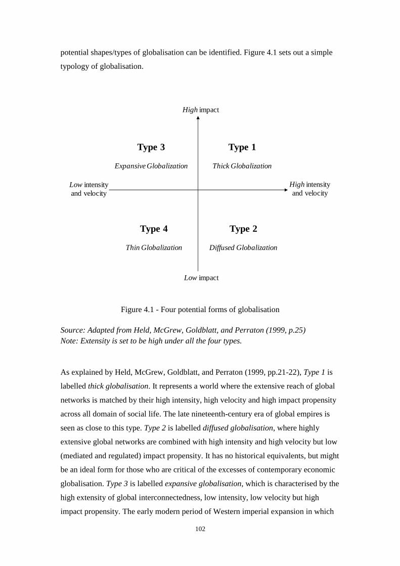
102
potential shapes/types of globalisation can be identified. Figure 4.1 sets out a simple
typology of globalisation.
Figure 4.1 - Four potential forms of globalisation
Source: Adapted from Held, McGrew, Goldblatt, and Perraton (1999, p.25)
Note: Extensity is set to be high under all the four types.
As explained by Held, McGrew, Goldblatt, and Perraton (1999, pp.21-22), Type 1 is
labelled thick globalisation. It represents a world where the extensive reach of global
networks is matched by their high intensity, high velocity and high impact propensity
across all domain of social life. The late nineteenth-century era of global empires is
seen as close to this type. Type 2 is labelled diffused globalisation, where highly
extensive global networks are combined with high intensity and high velocity but low
(mediated and regulated) impact propensity. It has no historical equivalents, but might
be an ideal form for those who are critical of the excesses of contemporary economic
globalisation. Type 3 is labelled expansive globalisation, which is characterised by the
high extensity of global interconnectedness, low intensity, low velocity but high
impact propensity. The early modern period of Western imperial expansion in which
High intensity
and velocityLow intensity
and velocity
High impact
Low impact
Type 1
Thick Globalization
Type 2
Diffused Globalization
Type 3
Expansive Globalization
Type 4
Thin Globalization

103
European empires had acquired a tentative global reach with considerable
intercivilizational impacts comes closest to this type. Type 4 is labelled thin
globalisation in so far as the high extensity of global networks is not matched by a
similar intensity, velocity or impact propensity. The early silk and luxury trade
circuits connecting Europe with China and the East have close parallels with this type.
It is worth noting that, even though the four types are somehow segregated in Figure
4.1, globalisation could transit from one form to another over time. In other words,
every era of globalisation builds on others, since absolute discontinuities do not exist
in human history. Hence there is an implicit temporal dimension to Figure 4.1.
Keohane and Nye Jr (2000, p.77) even argue that globalisation is the process by
which globalism becomes increasingly (from thin to) thick.
Figure 4.1 only presents four broad types of globalisation, while not leaving out many
different configurations within each type. The actual historical form of the
contemporary globalisation, or its exact position on Figure 4.1, depends on the values
of each spatio-temporal dimension. Hence, quantitative research is appropriate for
making the enquiry into the magnitude of each dimension, as long as the measurement
is clearly defined.
Recalling that the current research primarily concerns the concept of
‘interdependence’ (or ‘interdependency’), the intensity, velocity and impact
propensity dimensions are particularly relevant to empirical models. Adding the
extensity dimension, highly extensive interdependence would be a good interpretation
of globalism.
4.3 Economic Globalisation
Albeit a multidimensional phenomenon, globalisation is first and foremost understood
from the economic perspective. According to Panić (2003, p.4), the contemporary
process of globalisation that has gathered momentum since the 1970s is dominated by
economic considerations and developments, and it is associated with the economic
aspects of what is regarded as an irreversible trend towards greater international
integration and interdependence. Nevertheless, as Hirst and Thompson (2003, p.99)
suggest, ‘we can only begin to assess the issue of globalisation if we have some
relatively clear and rigorous model of what a global economy would be like’. The

104
current research thus place emphasis on the economic perspective, from which the
empirical econometric model (see Chapter 5) will be constructed.
Economic globalisation is generally specified in reasonably precise terms as ‘the
emergence and operation of a single, worldwide economy’ (McGrew, 2011, p.278). It
is measured by referencing to the growing extensity, intensity, and velocity of
worldwide economic interactions and interconnectedness, from trade, through
production and finance, to migration (McGrew, 2011, p.278). Economic globalisation
entails not only the openness of national economies, but also the integration and
interdependence between economies, although the concepts of openness, integration
and interdependence are highly compatible with spatially confined (or compressed)
occasions (i.e., the three concepts can also be applied to regional settings).
4.3.1 The Driving Forces
Economic globalisation can be seen following two interrelated paths of development
(see Panić, 2003, p.5). The first one is labelled institutional integration, where the
widespread liberalisation of international trade and capital flows has been initiated by
governments. The other one is labelled spontaneous integration, where the
international division of labour is achieved mainly through the actions of transnational
enterprises in pursuit of their corporate interests and objectives. It is claimed that what
distinguishes the contemporary globalisation from its earlier versions is the
spontaneous integration, since the world economy is now dominated by
transnationals and the penetration of transnationals into virtually every sector of
economies is far greater than before 1970s (Panić, 2003, p.5).
Whatever the pathway through which economic globalisation evolves is, the process
is driven by certain underlying forces, without which cross-countries interaction and
integration would not be made possible. Identifying the engines (or the prerequisites)
of economic globalisation, especially in the contemporary context, can be difficult and
tricky. As McGrew (2011, p.297) remark, ‘to date, no discrete or singular
globalisation theory – which seeks to provide a coherent and systematic account of its
causes, consequences, and developmental trajectory – can be said to exist’. Generally,
explanations of economic globalisation centre on three deeply interrelated forces,
namely technics (technological change and social organisation), economics (markets
and capitalism), and politics (ideas, interests, and institutions) (McGrew, 2011,

105
p.295). In addition, culture (cultural and demographic trends) is also considered as a
distinct force by Fayed and Fletcher (2002).
Technics Technics is vital to any account of globalisation. The developments of
modern communication and transport technologies allow time and space to be
compressed, so that a ‘shrunk’ globe can be formed (McGrew, 2011, p.295).
Specifically, the advancements in communication technologies have helped to spread
information and knowledge throughout the world, at much lower costs especially
since the 1980s (Azarya, 2004; McCann, 2008). As noted by Fletcher and Westlake
(2006) in the context of tourism, communication and information are the lifelines of
an industry that sells its product on faith and whose service providers are
geographically dispersed. Take computerised reservations systems (CRS) as an
example, they are believed to enhance small and medium-sized enterprises’ (SMEs)
profitability (Fletcher & Westlake, 2006). The use of modern communication and
information technologies in connection with various forms of integration (e.g.,
vertical, horizontal) extends the value chain of airline, hotels and tour operators
(Smeral, 1998). Meanwhile, the improved transportation facilities and services make
it more feasible and less costly for physical movements of not only goods (Fayed &
Fletcher, 2002) but also people between countries (Neumayer, 2006). More
profoundly, the technological change has driven liberalisations especially in the
financial sector, where financial markets scattered around the world are connected and
transactions are carried out 24/7 on a real-time basis. In a word, technics has
substantially facilitated international trade and shaped the transnational and global
organisation.
Economics The logic of economics explains globalisation from the perspective of the
market dynamics and the imperatives of capitalism (McGrew, 2011). On the one
hand, drawing on the neoclassical economic theories, the market dynamics logic
considers globalisation as a direct consequence of market competition. Briefly
speaking, free trade allows countries to maximise their welfare based on their
comparative advantages, whereas market forces and global competition enable goods
and services to be produced efficiently at a minimum cost. Consequently, vertical
integration is becoming commonplace. Meanwhile, economic convergence ensures
the key financial indicators such as interest rates to become equalised so that the cost
of financial leverage will be similar across countries. On the other hand, the logic of
106
capitalism follows the Marxist tradition that economic globalisation is driven by profit
seeking. The structural contradictions of capitalism – the tendency for overproduction
combined with the relative impoverishment of workers – and the insatiable
requirement for capital accumulation result in the expansion of corporations.
Therefore, from an economic perspective, globalisation is motivated by the continual
search for new markets, cheaper labour and new sources of profitability (McGrew,
2011). One fine example is the hospitality sector, where a hotel may pursue new
markets outside the local area, if it achieves the optimum share of a local or national
market and is faced with overcapacity (Fletcher & Westlake, 2006).
It is worth pointing out that, the expansion of economic activities is not without
backlash. One of the obstacles or counter-trends to the globalisation process is the
economic crises in recent years (Cohen, 2012). To bring the government finances
under control, austerity programmes have been instituted, which have been met with
severe popular protests around the globe, even as a growing distrust of, and
resentment against, the leading financial institutions of the prevailing capitalist system
(Cohen, 2012). The economic forces (the market dynamics and the imperatives of
capitalism) are by no means isolated from other forces. They are indeed set in motion
alongside such changes in the political and ideological domain as liberalisation (see
for example, Fayed & Fletcher, 2002; Stabler, Papatheodorou, & Sinclair, 2010;
Steger, 2005).
Politics The politics primarily concerns the ideological infrastructure of globalisation.
As noted by McGrew (2011, p.296), almost all accounts of contemporary
globalisation make reference to the rise and dominance of neoliberal ideology
throughout the OECD world, along with its associated policies of liberalisation,
deregulation and privatisation. Since the 1970s, the dominant political trend in OECD
states has been towards the liberalisation of national economies and the easing of
restrictions on capital mobility (McGrew, 2011, p.296). Governments, or rather states,
have been instrumental in establishing the necessary national political conditions and
policies – not to mention the vital regional and global institutions, agreements and
policies. Promoted and advocated by a powerful configuration of domestic and
transnational coalitions and lobbies, economic globalisation is very much a political
construction or project (McGrew, 2011, p.296). Fayed and Fletcher (2002) place the
emphasis on the liberalisation in trade and investment, which is embodied by the

107
establishment of the General Agreement on Trade and Tariffs (GATT), the General
Agreement on Trade in Services (GATS), and policies promoting free current and
capital account transactions by International Monetary Fund (IMF). Economic
convergence is thus facilitated by the establishment of these political infrastructures
(Stabler, Papatheoorou, & Sinclair, 2010, p.251). Furthermore, McGrew (2011,
pp.296-297) highlights the hegemonic power and role of the United States in
economic globalisation by extending its strategic interests and domestic politics.
Nevertheless, globalisation may also help developing countries exit the poverty trap
(Stabler, Papatheodorou, & Sinclair, 2010, pp.251-252). Prominent examples include
the emerging economies in East Asia and Southeast Asia, and the BRICS countries.
However, the ongoing trend of liberalisation and deregulation is not without
resistance, especially with respect to the mobility of people. Despite some political
initiatives (e.g., the right to free movement of the European Union nationals1) to
facilitate the movement of people, in the meantime visa restrictions are ironically
implemented by governments to deter some unwanted foreigners as well as the influx
of immigrants from certain countries (Cohen, 2012; Neumayer, 2006). In
consequence, detrimental impacts of visa restrictions can be observed in the domains
of trade, investment as well as tourism (Neumayer, 2011; Song, Gartner, & Tasci,
2012).
Culture Culture also plays a vital role (Fayed & Fletcher, 2002), in addition to the
technics, economics and politics. The growth in population since World War II has
created a demand for all kinds of economic goods, and the fact that the population
increases have not been evenly spread among countries implies trade opportunities
(Fayed & Fletcher, 2002). Cultural factors, including cultural exposure (e.g., the
demonstration effect through media sources), have led to some degree of
homogenisation. This is sometimes termed as ‘McDonaldisation’, which according to
George Ritzer is ‘the process whereby the principles of the fast-food restaurant are
coming to dominate more and more sectors of American society as well as the rest of
the world’ (Pieterse, 1996). An ostensible interpretation of the term would
immediately centre on the primacy of American culture, from films, music and
modern art to casual clothing, fast food and sports (Lieber & Weisberg, 2002). Such
1 http://ec.europa.eu/social/main.jsp?catId=457

108
primacy is more evident alongside the spread of (American) English as an
international lingua franca (Lieber & Weisberg, 2002; Steger, 2013). In one way or
another, this American primacy is merely a manifestation of the United States’
hegemonic power in the cultural sphere, and it is bound to evoke resistance, conflicts
and even clashes between cultures. Anti-globalisation advocates celebrate the cultural
difference and allege that the biodiversity and the richness of human culture are
destroyed by the American corporate interests (Lieber & Weisberg, 2002; Pieterse,
1996).
As an activity intrinsically involving cultural exchange, tourism can generate
awareness of cultural difference by increasing cross-cultural communication (Pieterse,
1996), while cultivating cultural hybridisation that allows for the cohabitation and
integration of different cultures. Cultural exploration can be regarded as a dimension
of visiors’ motives to attend festival events (Crompton & McKay, 1997), though
culture itself is a key pull factor.
4.3.2 Manifestation of Economic Globalisation
Economic globalisation can be observed across various economic activities. ‘It is the
confluence of secular trends and patterns of world trade, capital flows, transnational
production, and migration that for globalists affirms the validity of the globalisation
tendency’ (McGrew, 2011, pp.279-280). Among others, trade, finance and migration
are the three domains where economic globalisation takes place, as widely recognised
by Abel, Bernanke and Croushore (2008, p.476), McGrew (2011, pp.279-290),
Stabler, Papatheodorou, and Sinclair (2010, p.251) and Tribe (2011, p.363).
International trade is seen as a source for developing countries to accumulate profits;
it helps to fuel economic growth and capital formation and also boosts employment
(Stabler, Papatheodorou, & Sinclair, 2010, p.251). Over the post-war period,
international trade has experienced unprecedented growth. According to the World
Trade Organisation (WTO)’s figures, world exports, measured as a proportion of
world output, were three times bigger in 1998 than in 1950; the ratio was estimated to
be 29% in 2001 and about 27% in 2005, compared to 17% in 1990 and 12.5% in 1970
(McGrew, 2011, p.280). A contrast took place in 2008-2009, when the world trade
collapsed tremendously. In comparison with 2008, the value of world trade in 2009
fell by an unparalleled 33% and volume by 22%, according to WTO and the World

109
Bank’s figures (McGrew, 2011, p.280). All major exporters, especially Japan and
China, recorded export declines by more than 20%, and few economies escaped the
collapse (McGrew, 2011, p.280). This reality in turn reflects the penetration of
international trade into a larger number of countries and sectors than at any time
before. Alongside the booming of international trade is the shift of manufacturing
capabilities from developed/industrialised economies to the newly industrialising
economies (NIEs) such as East Asia, while most OECD economies have increased
their trade in services dramatically (McGrew, 2011, p.281). These structural shifts
constitute a new pattern of specialisation (or division of labour), where production is
fragmented or outsourced such that firms can draw on worldwide networks of
suppliers that produce at the greatest economies of scale (McGrew, 2011, p.281).
Through such a mechanism, economies in different regions become more tightly
integrated. However, the global market is far from a perfectly integrated one yet.
Based on convergence tests borrowed from economic growth theories, Chortareas and
Pelagidis (2004) find that the degree of openness converged faster across countries
within a given region rather than at the global level. It indicates that trade integration
is still more of a ‘regional’ phenomenon than a ‘global’ one. One account is
protectionism, which is manifested by the existence of non-tariff barriers (NTBs),
even though tariffs among major countries have been greatly reduced by successive
trade agreements under the General Agreement on Tariffs and Trade (GATT)
(McGrew, 2011, p.282; Winham, 2011, p.139).
International finance used to be an adjunct to trade, as a necessary mechanism
enabling the exchange of goods and services. This direct association between trade
and finance began to dissolve in the nineteenth century and even started to become
irrelevant in the twenty-first century (McGrew, 2011, p.283). As a multiple of world
merchandise trade, annual foreign exchange turnover in 1973 was equivalent to twice
the value of annual world trade, whereas by 2008 it was equivalent to more than sixty
times (McGrew, 2011, p.283). Indeed, the expansion of global capital flows is
unparalleled. In comparison to trade, which had a compound growth rate of almost
10% over the period 1964-2001, trans-border financial flows grew at a compound rate
of almost 19% (Bryant, 2003, p.141, cited by McGrew, 2011, p.283). However, the
trans-border financial flows are highly uneven. The access to world financial markets
is predominantly open to developed economies and major emerging market

110
economies, while many of the poorest economies remain subject to, rather than active
participants in, the operations of these markets (McGrew, 2011, p.284). Despite such
unevenness, the empirical evidence still supports the trend of financial integration.
Econometric studies by Obstfeld and Taylor (1999, 2003, 2004) identify, among
others, a narrowing of interest-rate differentials between the major OECD economies
after 1960, as might be expected under conditions of high capital mobility and
openness (McGrew, 2011, p.284). Furthermore, there is considerable evidence that
capital controls have declined significantly since the 1970s for OECD states and the
1980s for most developed economies, in association with the shift to a floating
exchange rate regime after the dissolution of the Bretton Woods System (Obstfeld &
Taylor, 2004, p.165, cited by McGrew, 2011, p.285). Hence, even capital is by no
means perfectly mobile across countries, the dominant tendency has been in the
direction of greater, rather than less, financial integration. Accompanying such
tendency is a process of financial deepening (in terms of contagion of financial crisis,
or the synchronisation of financial markets and business cycles) (Obstfeld & Taylor,
2004, cited by McGrew, 2011, p.285). Not only the increasing synchronisation of the
major stock markets and stock market returns since the 1970s, but also the rapidity
with which the 2008 financial crisis spread across the globe together with its dramatic
consequences for almost all economies, have unequivocally manifested the significant
deepening of global financial integration over the past few decades (McGrew, 2011,
p.285).
Compared to capital and goods, labour is relatively immobile. The movement of
people, or migration, has been one of the less spectacular dimensions of globalisation
(Tribe, 2011, p.363). Nevertheless, as noted in an International Organisation of
Migration (IOM) report, ‘no country remains untouched by international migration’
(McGrew, 2011, p.289). The direction of flows of people is primarily from
developing countries to the developed ones. In 2005, migrants totalled around 190
million of the world’s population, more than twice the level of 1970 (at 82.5 million),
making up some 3% of the global workforce, but 9% of the workforce in the
developed world (Freeman, 2006, cited by McGrew, 2011, pp.289-290). Moreover,
the huge expansion of temporary workers moving between countries/regions,
facilitated by low-cost transport infrastructures, is additional to the official figures and
is of growing importance to certain sectors (e.g., construction and agriculture) in

111
many developed economies (Freeman, 2006, cited by McGrew, 2011, p.290). These
developments of migration reflect the tendencies towards the integration of distant
labour workers and are expected to produce convergence in wage rates (McGrew,
2011, p.290; Stabler, Papatheodorou, & Sinclair, 2010, p.251), which may happen
particularly for the skilled workers, and to produce overall a divergence between rates
for skilled and unskilled workers will be observed.
All in all, it is worth reiterating the role of the four driving forces of globalisation.
Without the advancement of technology, the expansion of the corporations, the
liberalisation of political infrastructure and the exchange of cultures, cross-country
interconnections would lose their momentum. So would the process of globalisation.
4.4 Globalisation and the Tourism Sector
International tourism has been regarded as an important aspect of international trade,
through which globalisation is manifested. Over the past six decades, tourism has
experienced continued and almost uninterrupted expansion – from 25 million
international arrivals in 1950, to 278 million in 1980, 527 million in 1995, and 1,133
million in 2014 – and become one of the largest and fastest-growing economic sectors
in the world (UNWTO, 2015). Fayed and Fletcher (2002) report that, tourism ranks
among the top five export categories for 83% of countries covering Europe, the
Middle East and the Americas. According to the World Bank’s World Development
Indicator database1, tourism receipts accounted for 5.5% of worldwide total exports in
2011, and tourism expenditures accounted for 5.2% of worldwide total imports in that
year, although the percentages were even higher in 2005, at 6.5% and 6.2% for
receipts and expenditures, respectively.
Given the vital role of tourism in the world economy, it is no wonder that the
hyperglobalist position can often be found in tourism research (for example, Fayed &
Fletcher, 2002; Hjalager, 2007; Sugiyarto, Blake, & Sinclair, 2003; Vanhove, 2001).
In Encyclopedia of Tourism, globalisation is mainly interpreted from an economic
perspective: tourism is perceived to have long been ‘global’ in that tourists have
visited other countries, and in that the boom in mass tourism in the modern context
has been facilitated by transnational corporations (such as airlines and hotel chains)
1 World Development Indicators: Travel and Tourism, World Bank
(http://wdi.worldbank.org/table/6.14)
112
and the liberalisation of economic policies (such as foreign exchange); the result of
globalisation is elaborated through the economic benefits/loss of tourism (Jafari,
Baretje, & Buhalis, 2000, pp.254-256). For the hyperglobalizers, tourism is a force
working in favour of the global market and the global society (Munar, 2007). Tourists
are, in their opinion, consumers that bring the culture of consumerism to developing
countries. As such, tourism becomes the recipe for economic growth and facilitates
the forming of a global market. Tourism also contributes to the rising of a global
society, and is seen as a force of homogenization of the world. For the pessimist camp
of the hyperglobalizers, tourists help to expand a global society that represents the
Western culture dominating the world (Munar, 2007).
However, as in the globalisation debates, the existence of a global tourism market is
yet to confirm. The sceptic position in tourism research, though less prominent when
compared with the hyperglobalist, characterises international tourism from the
perspective of regionalisation, or even localisation. It is noted that, based on Vellas
and Bécherel (1995), tourism movements were dominantly domestic, and especially
in Europe the travel flows concentrated on intra-Europe on destinations (Munar,
2007). In much of the tourism literature, there is a preference for the use of
international tourism, rather than global tourism, in order to stress the importance of
the national framework (Munar, 2007). In the absence of a global market, tourists are
thus perceived as homogenised consumers of one country, and national typification
applies to tourists when they travel abroad.
From a transformationalist point of view, tourism is understood as an expression of
modernity, in which the root to globalisation is present (Munar, 2007). As cited by
Munar (2007), Urry (1995, p.141) argues that ‘central to the idea of modernity is that
of movement, that modern societies have brought about striking changes in the nature
and experience of motion or travel…in many ways the modern world is inconceivable
without these new forms of long-distance transportation and travel’. As such, ‘global’
and ‘tourism’ are not two separate entities, but part and parcel of the same set of
complex and interconnected processes (Urry, 2002, p.144, cited by Munar, 2007).
Tourism, as with the globalisation, is deeply rooted in history. It is the increase in
intensity and in extensity of tourism that makes a difference between different époques
of human history (Munar, 2007). On the concept of tourist, the transformationalist
position sees tourists as global citizens, where citizenship moves to where the person
113
moves. Their rights and duties are not rooted but mobile; they are not only consumers,
and not only national representatives of their country of residence (Munar, 2007).
In the context of globalisation, the development of international tourism is generally
observed from either the demand side or the supply side. The forms of international
tourism demand in history, as exemplified in the Encyclopedia of Tourism, include
medieval pilgrimages, grand tours of Europe in the eighteenth century, package tours
of Europe in the mid-nineteenth century, and ship-based travel in the early twentieth
century to remote destinations. Tourism demand grew even massively following the
advent of jet airplanes in the early 1960s (Jafari, Baretje, & Buhalis, 2000, p.255).
In response to the increasing tourism demand, national economies at destination
countries are heavily impacted. On the one hand, the economic leakages through
outbound tourism (i.e., tourism imports) by residents from developed countries often
bring in a net loss on the country’s tourism account (i.e., trade deficit on the balance
of payments). On the other hand, many developing countries receive net currency
inflows (i.e., trade surplus) as a result of diversifying their industries into tourism or a
result of attempting to gain additional tourism receipts (i.e., tourism exports) by
attracting more tourists from abroad (Stabler, Papatheodorou, & Sinclair, 2010,
p.239). The flows of tourists, accompanied by the commodity flows and monetary
flows, embody the extensive interactions between countries in the era of
contemporary globalisation. Hence, from an economic perspective, international
tourism can raise or lower a country’s dependence upon other countries and can
particularly be of importance to developing countries (Jafari, Baretje, & Buhalis,
2000, p.255; Stabler, Papatheodorou, & Sinclair, 2010, p.237). It is well recognised, at
least in theory, that international tourism can bring in income, create jobs, spur local
investments, diffuse technologies and thus promote economic growth (Fayed &
Fletcher, 2002; Schubert, Brida, & Risso, 2011; Stabler, Papatheodorou, & Sinclair,
2010, p.237).
As the national economy of a country can benefit from and even rely on its
international tourism sector, it is of interest to explain in the first place why and under
what circumstances a country chooses to specialise in international tourism. Stabler,
Papatheodorou, and Sinclair (2010, pp.238-243) revisit the traditional international
trade theories on comparative advantage, namely the Ricardian theory and the

114
Heckshcer-Olin (H-O) theorem. According to the Ricardian theory, the pattern of
trade is determined by the differences in the relative efficiencies of production
between different countries. The notion of comparative advantage states that, even if
a country is more efficient in absolute terms in producing a range of goods than
another country, gains from trade can be obtained if it focuses on the production and
export of the goods in which it has relatively higher efficiency. The Heckscher-Olin
(H-O) theorem, rather than exploring the efficiencies of production, posits that it is a
country’s endowments of factors of production (such as labour, capital, land and
natural resources) that determine its comparative advantage. Hence, it is theoretically
predicted that countries with a large supply of labour and with abundant land and
natural resources are more likely than those with less labour and natural resources to
specialise in tourism.
From the supply side, the boom in mass tourism has led to and been facilitated by the
increased involvement by transnational corporations (TNCs), including airlines,
hotels, tour wholesalers, tour operators, travel agents and car rental companies, which
are characterised by high levels of vertical and horizontal integration (Jafari, Baretje,
& Buhalis, 2000, p.255). Particularly, evidence has been found to support the view
that international fragmentation of production is prevalent in tourism service
production, and to resonate with the explanation for tourism specialisation based on
comparative advantages (Nowak, Petit, & Sahli, 2009). In exploring the motives for
expanding business overseas, Stabler, Papatheodorou, and Sinclair (2010, pp.253-254)
follow the OLI theoretical framework. The ‘O’ represents ownership, which argues
the underlying reason why a company extends its presence abroad is to enjoy
ownership advantages. These include capital and human resource endowments,
intellectual property rights and patents. The ‘O’ allows a company to access into
product and factor markets and exercise its oligopolistic and oligopsonistic power. It
is also associated with a company’s effort in diversifying business risk. The ‘L’ means
location, which concerns with the access to specific foreign country resources and
positive business environments such as high-quality/low-cost labour force, adequate
infrastructure, tax concessions and government funding. The presence in foreign
markets also assist in overcoming trade barriers and/or other protectionist
impediments and in reducing the cognitive and psychological distance. The ‘I’ refers
to internalisation. It allows a company to drastically reduce transaction costs in

115
acquiring inputs and to minimise uncertainty by exercising direct control over its
intangible assets, such as logos, image and brand names.
As noted in Encyclopedia of Tourism (Jafari, Baretje, & Buhalis, 2000, p.255),
international tourism is dominated in both demand and supply sides by developed
countries. Most tourist flows originate and take place between developed countries,
while tourism developing countries is dominated by tourists from developed countries
(Keller, 2000; Jafari, Baretje, & Buhalis, 2000, p.255). As a result, the economic
policies and the state of the economy in developed countries have profound impacts
on destinations around the globe, though the dominance of developed countries in the
international tourism sector is facing challenges from emerging countries. Given the
economic benefits brought by international tourism, the impact of tourism on
developing countries in the context of globalisation is therefore worth highlighting.
4.5 Economic Interdependencies of International Tourism Demand
Principally categorised as a form of international trade (Artus, 1972; Gray, 1966;
Smeral & Witt, 1996), in the first place international tourism involves movements of
people. It is the consumers instead of the goods or services that are transported across
borders, and tourism consumption/transaction occurs simultaneously with tourism
production (Song, Li, Witt, & Fei, 2010). The three domains of globalisation, i.e.,
international trade, international finance and migration, are deeply and inherently
embedded in tourism activities. As far as tourism demand is concerned, tourism
markets (or countries) are highly interconnected and interdependent. The implications
is, as described by Panić (2003, p.8) in the context of economic integration, ‘When
international economic interdependence reaches a certain level, what happens in one
group of economies may have a major impact on another group – even when the
volume of direct trade between the two is small – through the effect on a third group
with which both these groups trade heavily.’ To model and forecast tourism demand
for destination countries in a global setting, the understanding of the
interdependencies between tourism demand is a prerequisite.
While economic globalisation sets out the backdrop, it is the economic
independencies that become the focus of the current research, as mentioned in Section
4.2. The following sections provide a detailed interpretation of economic
interdependencies in the context of international tourism.

116
4.5.1 Impacts of Inbound Tourism
From the perspective of a destination country, international tourism has long been
perceived to have active impacts on the local economy and communities. The
economic impact of tourism is primarily understood in terms of income and
employment generation. This is often associated with the multiplier effect, which is
used to capture the economy-wide final benefits (sales, output, income, employment,
etc.) in comparison to the initial change of tourism demand. In brief, the expenditure
by inbound tourists not only brings direct economic benefits (i.e., direct effects) to
tourism-related businesses (e.g., hotels, restaurants and attractions), but also indirect
and induced effects onto the local economy (Stabler, Papatheodorou, & Sinclair, 2010,
pp.209-211). The indirect effects capture the economic benefits that local suppliers to
the tourism-related businesses (e.g., farmers, manufacturers and public utilities)
receive via the backward linkages between sectors. The income received through
direct and indirect involvement in tourism will then be re-spent by both the tourism-
related businesses and the suppliers for their own consumption as well as leisure
activities, creating knock-on effects on the local economy (i.e., induced effects).
Hence, considering the indirect and induced effects, the initial direct economic
benefits are multiplied.
Apart from income and employment generation, other economic impacts at the
macro-level are also discussed in the literature, mainly concerning the causal
relationship between inbound tourism demand and local economic growth. The logic
has generally been that, tourism is a significant foreign exchange earner; it plays an
important role in spurring investments in infrastructure and indirectly stimulates other
industries in the economy; it can cause positive exploitation of economies of scale; it
is also an important factor of diffusion of technical knowledge (Schubert, Brida, &
Risso, 2011). These beliefs that inbound tourism can promote local economic growth
are termed the Tourism-Led-Growth (TLG) hypothesis. Numerous empirical studies
have been put forth to investigate the validity of this hypothesis (for example,
Balaguer & Cantavella-Jorda, 2002; Belloumi, 2010; Kim, Chen, & Jang, 2006;
Narayan, Narayan, Prasad, & Prasad, 2010; Schubert, Brida, & Risso, 2011; Seetanah,
2011). The results are, however, rather inconclusive. While many studies confirm a
unidirectional causality running from inbound tourism demand to real GDP growth in
certain countries (and even find evidence of bidirectional relationship, for example,
117
Kim, Chen, & Jang, 2006), in some other studies no co-integration relation can be
detected (for example, Katircioglu, 2009). A similar thread of research follows the so-
called TKIG hypothesis, which is a variation of the TLG hypothesis by adding capital
formation as a channel of stimulating economic growth, i.e., tourism exports →
capital goods → imports growth (for example, Nowak, Sahli, & Cortes-Jimenez,
2007). Again, the hypothesis is not always supported by empirical evidence, and its
validity is conditional on the country under study (Song, Dwyer, Li, & Cao, 2012).
A straightforward implication of the mixed empirical results is that tourism does not
always contribute to local economic growth. In fact, it is not uncommon to find
studies that discuss the detrimental effects of tourism on local economy. Since the
early literature, researchers have noted that a tourism boom may lead to ‘de-
industrialisation’ (Copeland, 1991; Holzner, 2011; Nowak & Sahli, 2007). This
phenomenon is often termed the ‘Dutch Disease’ effect. It is indicated that tourists
mainly consume local amenities and non-tradable goods, such as heritage and cultural
facilities, nightlife, restaurants and shopping amenities. A tourist boom tends to raise
the demand for and hence the prices of these non-tradable goods, expanding their
production at the expense of the tradable sectors and, in particular, the manufacturing
sector (Chao, Hazari, Laffargue, Sgro, & Yu, 2006; Stabler, Papatheodorou, &
Sinclair, 2010, p.207). In addition, in the case where supplies of the non-tradables as
well as the tradables are relatively inelastic (for example, under full employment and
imperfect factor mobility, factors of production are not able to shift between sectors in
the short and medium term), the extra demand resulting from an expansion of tourism
would inevitably push up local prices of all goods and services. Furthermore, when
the local prices go up to a certain level, the attractiveness of the destination
diminishes. The case of demand pressure caused by tourists is exemplified by
Albalate and Bel (2010), who based their study on data of 45 European cities. They
found that if there was supply constraint, the additional demand for public transport
by inbound tourists could impose extra costs on local residents due to congestion,
even if the tourism receipts could provide some additional funding for the services.

118
Figure 4.2 - Impacts on local economy by inbound tourism
Source: the author
Given the profound impacts of tourism on destination countries’ economy and the fact
that tourist flows are heavily influenced by economic factors in the source countries
(as informed in Chapter 2), it is implied that destination countries’ tourism sector and
the overall economic performance can be susceptible to external economic climate.
Figure 4.2 visualises the role of tourism in connecting the world economy to
destination country’s economy. Tourists from a specific source country are subject to
such underlying influencing factors as income (denoted by GDP), consumer prices
and exchange rate in their own country and also oil price (a global common factor that
proxies the travel cost). Even though to a large extent the evolution of GDP, consumer
prices, and exchange rates follows a trajectory that differs from country to country,
the reality that countries are now more and more interconnected indeed gathers these
individual economic developments towards a (more or less) unified direction. As
such, the fluctuations of country-specific economic factors tend to synchronise across
borders, contributing to the forming of worldwide economic climate1. The
1 This is related to the synchronisation of business cycles and will be dealt with in Section 4.6.1.
Country-specific economic
factors:
- GDP
- Own price (exchange-rate-
adjusted consumer price index))
Global common factor
- Oil price
Economic factors:
- GDP
- Own price (exchange-
rate-adjusted consumer
price index)
Inbound tourism demand (i.e., exports)
Impacts on local economy
Destination Country Rest of the World
Tourist flows
World economy

119
consequence is that a destination country inevitably faces a collective external force1
which affects both its tourism sector and local economy, whereas in turn it has no or
only marginal influence over the external economic environment. From a theoretical
point of view, the collective external force (i.e., world economy) is said to be
exogenous to the local economy of the destination country.
The Assumption of Small Economies
In close association with the dominant influence of external environment on a
destination country is the concept of small economies, which constitutes a major
assumption for economic analysis. It is generally understood that a small economy
takes its external environment as pre-determined, and it has no control or influence
over the evolution of the external environment. In practice, it is difficult to find a
single yet satisfactory definition of small economies, be it population, geographical
size or GDP, because size (big or small) is a relative concept (Commonwealth
Secretariat, 2000, p.3). However, certain characteristics and implications of small
economies tend to be shared between a great many countries, such that even partial
possession of those attributes is often sufficient to justify the appropriateness of this
assumption in theoretical and empirical discussions.
The report by Commonwealth Secretariat (2000, p.5) lists seven common
characteristics among small economies, i.e., remoteness and insularity, susceptibility
to natural disasters, limited institutional capacity, limited diversification, openness,
access to external capital, and poverty. Specifically, it is worth highlighting some of
the implications with regard to limited diversification and openness of small
economies. As mentioned by Commonwealth Secretariat (2000, p.10) and Schubert,
Brida, and Risso (2011), small economies often opt for tourism as their development
strategy, because of their lack of diversification resulting from resource scarcity.
Citing World Bank’s data in the late 1990s, Commonwealth Secretariat (2000, p.10)
find that the exports in the Pacific and the Caribbean islands tended to concentrate on
services in tourism, with it constantly accounting for the highest or second highest
1 Here and hereafter, world economy, worldwide economic climate and external force are generally
synonymous in the current research. It can be represented by the aggregate of each country’s economic
factors, although the method of aggregation is open to discussion. Nevertheless, a weighted average of
each country’s economic factors (such as GDP and CPI) would be a simple and appropriate proxy. The
technical treatment of how to capture the worldwide economic climate will be discussed in the next
chapter.

120
percentages of total exports. The active involvement in international tourism reflects
the fact that small economies are highly open to trade, which means that they have a
large stake in a stable, rule-based, world trade environment. Even minor disruptions in
world markets (such as fluctuating demand and prices for exports) can have a
significant impact on their economies (Commonwealth Secretariat, 2000, p.9).
Accordingly, the extreme openness of small economies may entail a high degree of
vulnerability to external shocks, which is attributable to interrelated geographic,
demographic and economic factors, and inevitably attract income volatility (Ocampo,
2002; Schubert, Brida, & Risso, 2011).
In tourism economics research, small economies (particularly island economies) are
often the subject as well as the setting of studies (for example, Chen & Chiou-Wei,
2009; Narayan, Narayan, Prasad, & Prasad, 2010; Santana-Gallego, Ledesma-
Rodríguez, & Pérez-Rodríguez, 2011; Schubert, Brida, & Risso, 2011; Seetanah,
2011). This is not surprising, because the specialisation in and dependence on
international tourism are not uncommon among small economies1. They are thus
perfect samples to test for the causal relationship between tourism and economic
growth, for example, the Tourism-Led-Growth (TLG) hypothesis.
Within the ‘cohort’ of small economies, it is worth noting that not all of them are
alike. They can range in population from fewer than 50,000 people to more than 1
million people; in per capita income, from less than US$400 to more than US$9,000
(Commonwealth Secretariat, 2000, p.3). Hence, by nature small economies is rather
loosely defined and inclusive. Given that in reality many countries are open
economies with only limited influence over the worldwide economic climate, in most
cases it is appropriate to apply the small economies assumption when conducting
macroeconomic analysis, except for the case of USA due to its economic and political
dominance. In addition, admittedly extra care needs to be taken when applying the
assumption to major countries such as China, Germany, Japan and the UK, as these
economies are very active in shaping the worldwide economic landscape.
Nevertheless, the small economies assumption generally provides a convenient
yardstick to describe the setting in which a great many economies are operating.
1 However, logically the association between small economies and tourism indicates neither that all
small economies are tourism-oriented, nor that countries with a vigorous tourism sector are all small
economies.

121
Therefore, as is acceptable in macroeconomics studies (for example, Bussière,
Chudik, & Sestieri, 2009; Dees, Mauro, Pesaran, & Smith, 2007), the small
economies assumption is suitable for tourism demand analysis as well.
4.5.2 Spillovers via Outbound Tourism
From the perspective of a source country, outbound tourism has been an effective
channel through which the country contributes to the shaping of the world tourism
market and the worldwide economic climate. The mechanism is principally the same
as that described in Figure 4.2, although in the reverse direction.
Figure 4.3 - Spillover effects of outbound tourism demand
Source: the author
One of the direct implications in relation to outbound tourism demand is that, the
economic situation in the source country can be transmitted across borders via the
outbound tourist flows. For example, a temporary adverse shock (i.e., unexpected
event) to the source country’s GDP or unusual turbulences in the foreign exchange
market can result in contracted outflows of tourists. Consequently the destination
Country-specific economic
factors:
- GDP
- Own price (exchange-rate-
adjusted consumer price index)
Economic factors:
- GDP
- Own price (exchange-rate-
adjusted consumer price index)
Global common factor
- Oil price
Outbound tourism demand (i.e., imports)
Spillovers to foreign economies
Source Country Rest of the World
Tourist flows
Local economy
122
countries will feel the shock that originally takes place in the source country, because
less tourism income is registered. The theoretical inference of this welfare-decreasing
mechanism is shown by Schubert and Brida (2009), using a dynamic macroeconomic
equilibrium model. In short, the shock to the source country can be said to spillover to
foreign economies. Figure 4.3 visualises the process of spillover.
Still, cautions are worth to be taken that the effects of spillover on foreign economies
never be overstated under the small economies setting. It is in general not expected
that a shock to a ‘standard’ small economy would be able to create catastrophic
effects, unless it triggers a major economy that has more weights in the world
economy1. In fact, the spillover effects from a source country of tourists should be
understood in twofold. On the one hand, for the destination countries that are related
to the particular source market, the spillover directly affects their local economy, the
strength of which is commensurate with the market share of the source country. On
the other hand, for the countries that do not receive tourists from the particular source
market, the spillover contributes to the evolution of the generic worldwide economic
climate and becomes an integrated part of it, which ultimately impacts on all other
open economies around the globe. As such, if all the economies are seen as an
integrated ecosystem, then a source country can be said to be, to a certain extent,
endogenously related to the tourism sector as well as local economy of the other
countries.
The Balance between Outbound Demand and Inbound Demand
As a country can be a tourist receiving country and a tourist generating country at the
same time, an issue is raised that from a holistic point of view the outbound tourism
demand (i.e., tourism imports) relates to and to a certain extent co-moves with the
inbound demand (i.e., tourism exports). Figure 4.4 combines both Figure 4.2 and
Figure 4.3, showing the inherent connection between inbound and outbound tourism.
For country i, a small open economy, on the one hand the volume of tourist inflows
(i.e., inbound tourism demand) is exogenously determined by the world economy,
which represents the combination of each country’s economic factors. Hence, country
1 The on-going Eurozone debt crisis since late 2009 is an example where the sovereignty debt crisis in
small economies, such as Greece and Ireland, renders the threat that the crisis could be transmitted to
France and thus have disastrous implications to the world economy.

123
i’s inbound tourism demand co-moves or fluctuates along with the prevailing world
business cycles1. On the other hand, given the impacts of inbound tourism on local
economic factors, which in turn determine the outflows of residents (i.e., outbound
tourism demand), it can be implicated that, the higher the volume of tourist inflows to
country i, the higher the income (or GDP) and price level that country i may achieve,
making it more favourable for residents in country i to conduct outbound tourism, and
vice versa. In this sense, the fluctuations of outbound tourism demand are correlated
to those of the inbound tourism demand. Furthermore, the consumption of outbound
tourists becomes the medium through which country i’s business cycle is spilled over
to foreign economies and integrates with the world business cycle. However, despite
the underlying logic, co-movements between inbound and outbound tourism demand
may not necessarily be observable at all times, as the inflows and outflows of tourists
can be deterred by non-economic factors, such as visa restrictions.
All in all, the inbound tourism demand and outbound tourism demand embody the
extent to which a country depends on and is depended on by other countries. The
balance between inbound tourism demand and outbound tourism demand, i.e., the
balance of tourism services trade, indicates a country’s position against the others in
an interconnected world.
In the era of globalisation, the more integrated each economy is with another, the
higher level of co-movements between inbound and outbound tourism demand may be
observed, no matter whether within a particular country or across various countries.
Interdependencies are thus understood as an intrinsic attribute of the world tourism
market in the contemporary context. The implication of this reality is that, as with the
generic macro economies where synchronisation of business cycles can be observed
on a global scale, similar patterns of synchronisation may exist among the
international tourism sectors across different countries. This issue will be dealt with in
Section 4.6.1.
1 Business cycle refers to the short-run to medium-run fluctuations in aggregate production, trade and
other economic activities. It is generally depicted as the periods of expansions and contractions in the
level of economic activities (often in terms of GDP) around a long-run growth trend.

124
Figure 4.4 - Correlation between outbound demand and inbound demand
Source: the author
4.5.3 Complementary and Substitutive Relations between Tourism Demand
Apart from the dynamics between tourism demand and economic factors, as described
in Section 4.5.1 and Section 4.5.2, there exists mutual influence of tourism demand
between different destination countries. In brief, such mutual influence is understood
from the perspective of complementary effect and/or substitution effect.
In generic economic theory that concerns consumer demand, it follows that
goods/services are to some extent interrelated. They can be either complements or
substitutes to each other1 (Pindyck & Rubinfeld, 2013, pp.24-25; Snyder &
Nicholson, 2012, pp.171-172). On the one hand, if the consumption of one good is
accompanied by that of another good (for example, printers and ink cartridges, tea and
1 In the case where no interrelation exists, that is the change in price of one good has no effect on the
demand for another, it is said that the two goods are independent.
Tourist flows
Tourist flows
Country-specific
economic factors:
- GDP
- Own price (exchange-
rate-adjusted consumer
price index)
Economic factors:
- GDP
- Own price (exchange-
rate-adjusted consumer
price index)
Outbound tourism demand (i.e., imports)
Inbound tourism demand (i.e., exports)
Global common factor:
- Oil price
Country i Rest of the World

125
milk), it is said that the two goods are complements. More formally, a complementary
good is often defined as a good with a negative cross-price elasticity of demand,
which means the demand for the good is inversely related to the price of its
complement (for example, more ink cartridges would be sold if the printers become
cheaper)1. On the other hand, if the consumption of one good can be replaced by
another without compromising much in terms of quality and utility (for example,
margarine and butter, tea and coffee), it is said that the two goods are substitutes.
Accordingly, a substitute good is often associated with a positive cross-price elasticity
of demand, so that the demand for the good changes in the same direction as the price
of its substitute (for example, more tea would be consumed if the coffee becomes
more expensive).
In the context of international tourism, similar interrelations can be observed among
destination countries. Some destinations are complements, and the price drop in one
country may result in an increase of visitor arrivals to several neighbouring countries
because they can be visited on the same trip. One explanation can be that some
destinations are often bundled in a holiday package. One of these examples is the
bundle of Singapore, Malaysia and Thailand, which has been constantly popular with
Chinese tourists. Another explanation can be that some countries adopt a common
visa policy and abolish border control at their common borders, hence enabling a
cross-country trip during a single visit. The Schengen Area that comprises 26
European countries is a notable example. In contrast, the interrelationship of other
destination countries contains some elements of competition, because they are
somewhat perceived as substitutes. For example, the Spanish islands (Balearic,
Canary, etc.) and the Greek islands (Crete, Corfu, etc.) are both alluring places for
summer holidays, while in the winter, Austria, France and Switzerland are all ‘hot’
destinations for skiing. Tourists may well choose a destination after a price hike in the
alternative ones. Apparently, although defined by the cross-price elasticity, the
determination of the interrelationship between destination countries can be inherently
associated with non-economic factors that are supply side (destination) related and
tend to fall into the category of external inputs in Figure 2.2, for example, climate,
1 It is assumed that both goods are ordinary goods, which means for either good itself, the higher its
own price, the lower the demand for it. The same assumption applies to the case of substitute goods.

126
geographical proximity, cultural similarity, destination attractions/facilities, and/or
simply political reasons (e.g., visa policy).
Given the interrelationship between destination countries, it is implied that the
inbound tourism demand may be numerically correlated to one another. Tourist
inflows to a destination country tend to increase alongside an increase of demand for
its complements and/or a decline for its substitutes. In the literature, such
interrelationship between a destination and its alternatives can be explicitly modelled.
In many studies, a substitute price (or cross price) variable is constructed and
included in the tourism demand model, as explained in Section 2.4.41. For example,
France, Greece, Italy, Portugal and Spain are chosen by Li, Wong, Song, and Witt
(2006) as alternative destinations for UK’s outbound tourism; Indonesia, Malaysia,
Philippines, Singapore and Thailand are seen as substitutes by tourists from several
developed countries in Song, Witt, and Li (2003). The sign and value of the
coefficient on the substitute price variable, which represents the cross-price elasticity,
reveal the relationship between these alternative destinations (‘+’ means substitutes,
‘-’ means complements) and its magnitude. Generally, empirical evidence suggests
that the relationship is perceived differently from one origin country to another, and
its magnitude can evolve over time (for example, Li, Wong, Song, & Witt, 2006;
Song, Witt, & Li, 2003). Some other studies take a closer look at the substitution
effect, as this to a large extent reflects how keen the competition between destination
countries can be (Dwyer, Forsyth, & Dwyer, 2010, p.51; Li, Song, Cao, & Wu, 2013;
Mangion, Durbarry, &Sinclair, 2005). It is suggested that the cross-price elasticity can
be essential information for formulating pricing strategy, which in turn helps to
enhance a destination country’s competitiveness.
In sum, depending on the nature of their relationship, tourism demand for one
destination can be expected to co-move with that for another either directly or
inversely. In this sense, there exists certain levels of interdependencies between
destination countries that may ultimately be underpinned by non-economic factors.
1 To recapitulate, a substitute price variable is a weighted average index of prices in alternative
destinations.
127
4.6 Empirical and Theoretical Implications
The discussions in Section 4.5 delineate the mechanism behind the interdependencies
between tourism countries. In brief, these are driven by the interactions between
tourism demand and economic factors at home and abroad, and the
complementary/substitute nature of the relationship between tourism countries.
The understanding of the interdependencies, as stated at the outset of Section 4.5,
sheds some light on a more accurate tourism demand modelling practice. In the
meantime, it illuminates a better analysis of the current economic affairs that should
have far-reaching implications across borders.
4.6.1 Business Cycle Synchronisation
Interdependencies between countries, as described in great details in Section 4.5,
imply certain level of co-movements of economic activities on the global scale.
Similar co-movements can also be observed in the international tourism sector in the
wake of the recent global recession, even though there were additional disturbances
playing their parts at the same time.
Business Cycle Synchronisation
In general, business cycle refers to the fluctuations in aggregate economic activities,
which are usually in terms of gross domestic product (GDP), employment and so on,
over the short term (Mankiw, 2006, p.252). It comprises periods of expansions,
followed by recessions and revivals, in the level of output around the economy’s long-
term growth trend for more than one year and up to ten or twelve years (Abel,
Bernanke, & Croushore, 2008, pp.283-284; Sørensen & Whitta-Jacobsen, 2010,
pp.358-359).
In the era of increasing economic integration, the conventional wisdom is that cross-
border interdependences should lead to convergence of business cycles, although an
alternative view indicates the opposite, i.e., more asynchronous output fluctuations,
because the production of goods is highly specialized and country-specific (Canova,
& Ciccarelli, 2012). An explanation is, as summarised by Canova and Ciccarelli
(2012) and Derviş (2012), production cycles could be completely idiosyncratic since
they are linked to relatively long-term supply-side factors (e.g., capital accumulation,

128
technological catch-up, and demographics) while consumption cycles are perfectly
correlated since they are linked more to shorter-term demand-side factors.
Many studies under the labels of business cycle synchronisation, international
transmission mechanism, decoupling and recoupling and international contagion can
be found in generic economic literature (e.g., Artis, Fidrmuc, & Scharler, 2008;
Canova & Ciccarelli, 2012; Hamori, 2000; Sayek & Selover, 2002). In short,
contradictory evidence has been found. A notable study is conducted by Kose, Otrok,
and Prasad (2012). Based on the data for 106 countries over the period of 1960-2008,
they find that there has been a substantial convergence of business cycles among
industrial economies and among emerging market economies, but there has also been
a concomitant divergence (or decoupling) of business cycles between these two
groups of countries.
To explain the mechanism behind the transmission of business cycles (i.e., the trigger
and the path of transmission), two main hypotheses have been put forth: locomotive
hypothesis and common shocks (Bagliano, & Morana, 2010; Sayek, & Selover, 2002;
Selover, 1999). In economics, shocks refer to unexpected or unpredictable events that
have regional or global implications (either positive or negative) on the economy. The
concept of ‘shocks’ is often associated with business cycles, since it is the fluctuations
that are of interest. The locomotive hypothesis assumes that business cycles are
transmitted across countries via trade flows, capital movements, labour migration and
technological transfer. The impacts of income shocks, price shocks and interest rate
shocks have been examined under this hypothesis (Sayek & Selover, 2002). The
common shocks hypothesis concerns about the shocks that affect the majority of
countries worldwide, such as technological advancement and commodity supply
shocks (e.g., oil crisis in the 1970s). Regardless of which hypothesis to follow, it is
implied that a shock to any variable in a particular country can have impacts over
other variables in both the national economy and foreign economies.
Empirically, business cycles are often studied using the vector autoregression (VAR)
model (for example, Abildgren, 2012; Bagliano & Morana, 2010; Hamori, 2000;
Sayek & Selover, 2002). As reviewed in Section 3.2.2.1, one advantage of the VAR
model is that it is able to simulate the impacts of a shock through impulse response
analysis. In brief, an impulse response describes how one economic variable reacts

129
over time to a shock (or exogenous impulse) in another variable within a system that
involves a number of other variables as well.
A notable recent development in the VAR modelling practice has been the global
VAR (GVAR) model. It is first proposed by Pesaran, Schuermann, and Weiner
(2004). The novelty of GVAR lies in its ability to link up a large number of regional
systems into a unified global system, while avoiding the ‘curse of dimensionality’
discussed in Section 3.2.2.1. By treating variables as endogenously determined, the
model explicitly allows for the interdependencies that exist between national and
international factors. The applications of the GVAR model have been modelling the
international transmission mechanism via generic economic variables such as real
GDP, inflation, interest rates and exchange rates (e.g., Boschi, 2012; Bussière,
Chudik, & Sestieri, 2009; Chudik & Fratzscher, 2011; Chudik & Straub, 2010; Dees,
Mauro, Pesaran, & Smith, 2007; Galesi & Sgherri, 2009;N’Diaye & Ahuja, 2012;
Pesaran, Schuermann, & Weiner, 2004), and the applications in narrower scope are
not uncommon as well (for example, the housing market, Vansteenkiste & Hiebert,
2011; the labour market, Hiebert & Vansteenkiste, 2010).
In the context of tourism, studies concerning the business cycle of tourism demand
have been very limited, even though the earliest one dates back to the late 1970s, by
Schulmeister (1979). The general considerations of the existing studies have been that
a specific country’s tourism demand follows the economic fluctuations (e.g.,
Frechtling, 1982; Guizzardi & Mazzocchi, 2010) or that the variation of tourism
demand elasticities across different phases of the business cycle (Smeral, 2012).
However, few studies have considered the interrelationship between tourism
countries. Following the discussions since the beginning of the chapter, the
interdependencies between tourism countries mean that a country’s international
tourism demand (inbound and outbound) is highly sensitive to idiosyncratic shocks in
other countries and/or global common shocks. Examples of shocks that disrupt the
world tourism sector can be found in WTTC (2011), which summarises some
unprecedented global events throughout 2011. These include the economic instability
in the wake of the financial crisis and recession since 2008, the natural disasters such
as the nuclear accident in Japan after a devastating tsunami and the earthquake in
Christchurch in New Zealand, and the socio-political upheaval seen in North Africa
and Middle East (known as ‘Arab Spring’). It was expected that both tourism
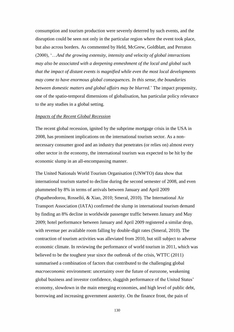
130
consumption and tourism production were severely deterred by such events, and the
disruption could be seen not only in the particular region where the event took place,
but also across borders. As commented by Held, McGrew, Goldblatt, and Perraton
(2000), ‘…And the growing extensity, intensity and velocity of global interactions
may also be associated with a deepening enmeshment of the local and global such
that the impact of distant events is magnified while even the most local developments
may come to have enormous global consequences. In this sense, the boundaries
between domestic matters and global affairs may be blurred.’ The impact propensity,
one of the spatio-temporal dimensions of globalisation, has particular policy relevance
to the any studies in a global setting.
Impacts of the Recent Global Recession
The recent global recession, ignited by the subprime mortgage crisis in the USA in
2008, has prominent implications on the international tourism sector. As a non-
necessary consumer good and an industry that penetrates (or relies on) almost every
other sector in the economy, the international tourism was expected to be hit by the
economic slump in an all-encompassing manner.
The United Nationals World Tourism Organisation (UNWTO) data show that
international tourism started to decline during the second semester of 2008, and even
plummeted by 8% in terms of arrivals between January and April 2009
(Papatheodorou, Rosselló, & Xiao, 2010; Smeral, 2010). The International Air
Transport Association (IATA) confirmed the slump in international tourism demand
by finding an 8% decline in worldwide passenger traffic between January and May
2009; hotel performance between January and April 2009 registered a similar drop,
with revenue per available room falling by double-digit rates (Smeral, 2010). The
contraction of tourism activities was alleviated from 2010, but still subject to adverse
economic climate. In reviewing the performance of world tourism in 2011, which was
believed to be the toughest year since the outbreak of the crisis, WTTC (2011)
summarised a combination of factors that contributed to the challenging global
macroeconomic environment: uncertainty over the future of eurozone, weakening
global business and investor confidence, sluggish performance of the United States’
economy, slowdown in the main emerging economies, and high level of public debt,
borrowing and increasing government austerity. On the finance front, the pain of

131
credit crunch in one region could partly (if not fully) be felt by another region. As a
result, the financial activity and credit growth are likely to remain subdued in many
economies, restricting the expansion capacity of tourist enterprises (Papatheodorou,
Rosselló, & Xiao, 2010). In addition, as noticed by Papatheodorou, Rosselló, and
Xiao (2010), the recession has also led to a downturn in the world labour market. The
International Labour Organisation (ILO) highlighted that worldwide unemployment
rate, one of government’s management targets, could reach between 6.5% and 7.4%
in 2009 (Papatheodorou, Rosselló, & Xiao, 2010), reflecting the far-reaching impacts
of the recession.
The Roles of Emerging Economies
One trend emerging from the recession is that developing economies are playing a
more and more important role in the world economy. It is now formally recognised by
the G7 ancien régime that major developing countries are important pillars of the
world’s financial system (Papatheodorou, Rosselló, & Xiao, 2010).
Outbound tourism from developing countries can help to restore reciprocity and
stability of international trade. This is evidenced by the statistics. Over the last decade
China has shown the fastest growth with respect to expenditure on international
tourism, thanks to rising disposable incomes, a relaxation of restrictions on foreign
travel and an appreciating currency (UNWTO, 2013). In 2009, when the world
economy was severely hit by the financial crisis, China’s tourism expenditure
registered a whopping 21% increase, whereas other top spenders saw near zero or
even negative growth (UNWTO, 2010). Indeed, in 2005 China ranked seventh in
international tourism expenditure, and has since overtaken Italy, Japan, France, the
UK, the USA and Germany, to become the world’s first place top spender in 2012
(UNWTO, 2013). Another emerging economy showing an impressive advance is
Russia. It moved up two places in 2012 to the fifth on the back of a 37% growth
(UNWTO, 2013).
Such up-rise of developing countries is bound to affect not only the pattern of
international trade, but furthermore the exchange rate regime. Although it is
premature to argue that the Chinese yuan will eventually mount to a global
dominance, it is clear that the US dollar is less exclusively relied on for international
business transactions, including tourism (Papatheodorou, Rosselló, & Xiao, 2010). A

132
strong contender, the euro, which was expected to challenge the US dollar, is however
mired in the debt crisis of its member states. Nevertheless, the relative variation of
values of currencies would certainly change the landscape of global tourism markets.
Depreciations of US dollar and euro may bring some edge to the inbound tourism of
USA, and help Mediterranean countries (e.g. Spain, Italy, and Greece) maintain cost
advantage.

133
Table 4.2 - Top source countries for China’s inbound tourism
Ranking 2013 2012 2011 2010 2009
1 Korea Korea Korea Korea Japan
2 Japan Japan Japan Japan Korea
3 Russia Russia Russia Russia Russia
4 USA USA USA USA USA
5 Vietnam Malaysia Malaysia Malaysia Malaysia
6 Malaysia Vietnam Singapore Singapore Singapore
7 Mongolia Singapore Vietnam Vietnam Philippines
8 Philippines Mongolia Mongolia Philippines Mongolia
9 Singapore Philippines Philippines Mongolia Australia
10 Australia Australia Canada Canada Canada
11 Canada Canada Australia Australia Thailand
12 India Germany Germany Thailand UK
13 Thailand Thailand Indonesia Germany Germany
14 Germany Indonesia Thailand UK Indonesia
15 UK UK India Indonesia India
Note: 1) Countries in shade are among those modelled in the current research;
2) Hong Kong, Macao and Taiwan are excluded from the above list
Table 4.3 - Top destination countries for China’s outbound tourism
Ranking 2013 2012 2011 2010 2009
1 Korea Korea Korea Japan Japan
2 Thailand Thailand Malaysia Korea Korea
3 USA Japan Japan Vietnam Vietnam
4 Japan Cambodia Thailand USA USA
5 Vietnam USA USA Malaysia Russia
6 Cambodia Malaysia Cambodia Thailand Singapore
7 Malaysia Vietnam Vietnam Singapore Thailand
8 Singapore Singapore Singapore Russia Malaysia
9 Guinea-
Bissau Russia Russia Australia Australia
10 Russia Australia Australia Indonesia Myanmar
11 Indonesia Indonesia Indonesia Cambodia Indonesia
12 Australia Myanmar Italy UK UK
13 Myanmar Italy UK Canada Germany
14 Canada Canada Canada Germany France
15 UK UK Germany France Cambodia
Note: 1) Countries in shade are among those modelled in the current research;
2) Hong Kong, Macao and Taiwan are excluded from the above list
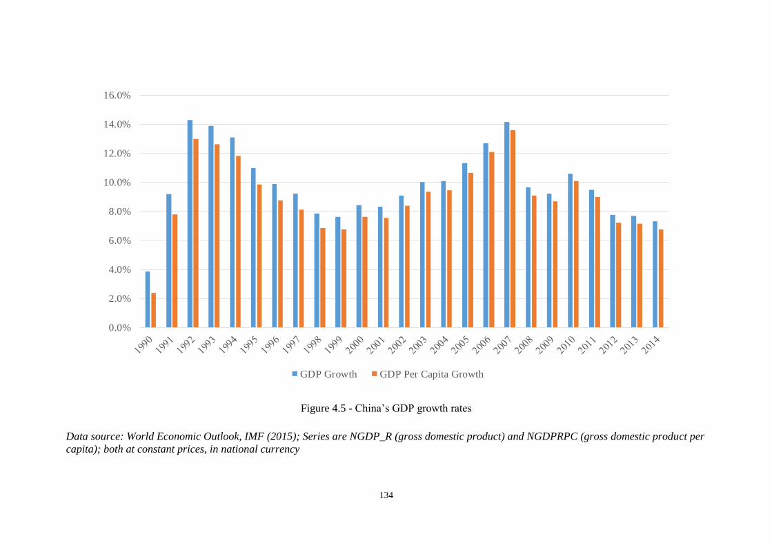
134
Figure 4.5 - China’s GDP growth rates
Data source: World Economic Outlook, IMF (2015); Series are NGDP_R (gross domestic product) and NGDPRPC (gross domestic product per
capita); both at constant prices, in national currency
0.0%
2.0%
4.0%
6.0%
8.0%
10.0%
12.0%
14.0%
16.0%
GDP Growth GDP Per Capita Growth
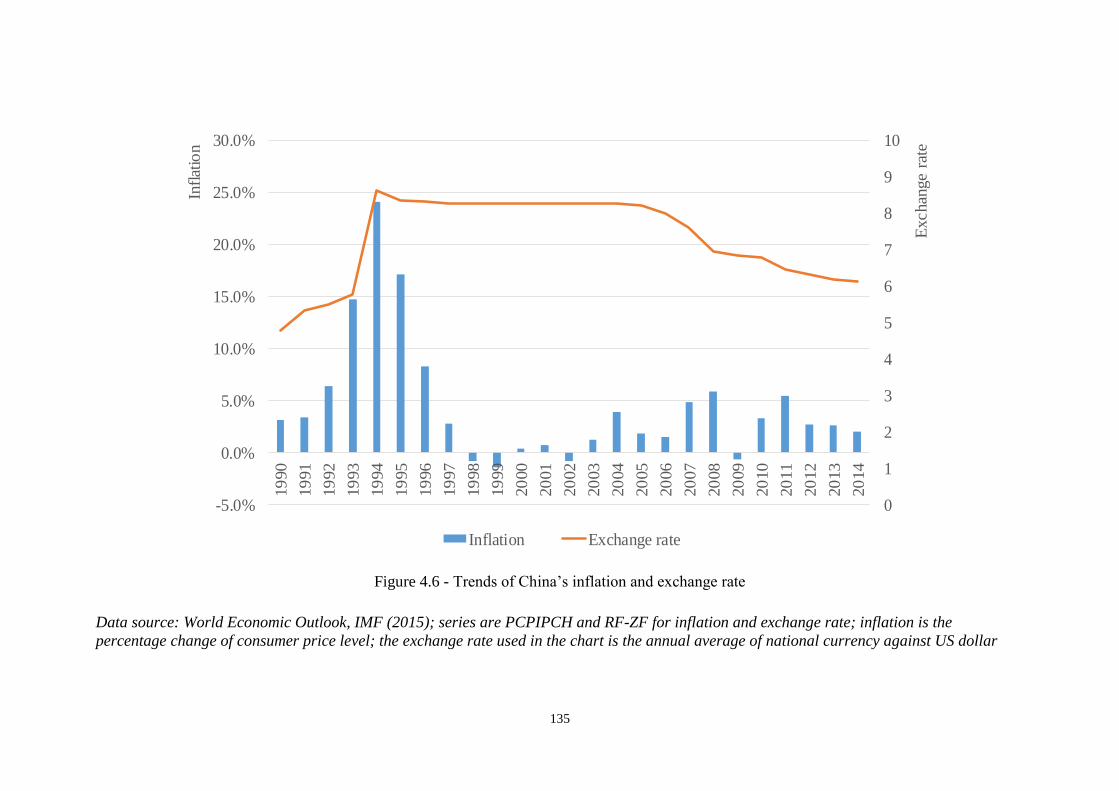
135
Figure 4.6 - Trends of China’s inflation and exchange rate
Data source: World Economic Outlook, IMF (2015); series are PCPIPCH and RF-ZF for inflation and exchange rate; inflation is the
percentage change of consumer price level; the exchange rate used in the chart is the annual average of national currency against US dollar
0
1
2
3
4
5
6
7
8
9
10
-5.0%
0.0%
5.0%
10.0%
15.0%
20.0%
25.0%
30.0%
19
90
19
91
19
92
19
93
19
94
19
95
19
96
19
97
19
98
19
99
20
00
20
01
20
02
20
03
20
04
20
05
20
06
20
07
20
08
20
09
20
10
20
11
20
12
20
13
20
14
Exchan
ge
rate
Infl
atio
n
Inflation Exchange rate

136
4.6.2 China as an Emerging Economy
China is one of the biggest economies in the world, in terms of gross domestic
product (GDP). Thanks to the unprecedented growth over the past few decades, China
has overtaken Japan to be the second largest economy ever since 20101. Figure 4.5
shows the growth rates of China’s GDP during 1990-2014, with early-1990s and mid-
2000s being the most impressive, easily beyond 10%. However, since 2008, China’s
economic growth has seemed to lose some momemtum. The growth rate was
staggering at around 8%, which is still a striking number. But it is apparent that the
Chinese economy will not grow as fast as before.
Alongside the extraordinary economic growth is the expansion of China’s
international tourism sector. According to the National Bureau of Statistics of China
(2015), the number of international tourist arrivals to China has grown from 43.685
million in 1994 to 128.49 million in 2014, whereas the resident departure from China
has seen an even steep growth, from 3.73 million in 1994 to 116.59 million in 2014
(all the numbers include tourists to and from Hong Kong, Macao and Taiwan). One of
the trends most discussed in the recent years is the increasing importance of Chinese
outbound tourists to the local economy in other major tourism countries (see also the
previous section). The Chinese market has become particularly relevant for businesses
to maintain competitive edge. Table 4.2 and Table 4.3 present the major source
countries and the major destination countries for China over the recent years, in terms
of the number of tourist arrivals. One observation from both tables is that many of the
countries are both top source markets and top destinations at the same time, reflecting
the close ties between China and those countries. Another observation is that China’s
international tourism sector (irrespective of inbound or outbound tourism) mainly
concentrates in short-haul markets, with many countries situating in Asia. It is logical
to expect that any economic changes in China could have notable impacts on those
short-haul markets.
As to inflation and exchange rate against the US dollar (see Figure 4.6), they had a
relative unsteady period in the early to mid-1990s. Inflation was unusually high
between 1992 and 1996, but has experienced less ups and downs since 2000s. For the
1 http://www.bbc.co.uk/news/business-12427321;
http://www.wsj.com/articles/SB10001424052748703361904576142832741439402

137
exchange rate, it is clear that since 2008 there has been a steady appreciation of the
Chinese currency. However, speculations came in the early autumn 2015 that the
Chinese renminbi (RMB) now faced devaluation1. Depreciating the currency is of
course helpful to boost China’s competitiveness in its exports. To this end, China’s
central bank allowed for a greater role of the market in determining the value of
RMB, which used to be heavily pegged against the US dollar. Such a move also fits
well into China’s long-term goal of establishing RMB as a major internationally
traded currency2. Now that the Chinese currency is expected to be included into the
basket of IMF’s special drawing right (SDR)3, which is a step forward for China to
achieve its goal, fears of devaluation are increasingly mounting4. All in all, the
exchange rate of the Chinese currency is likely to become more volatile. So is China’s
own price level (i.e., consumer price index adjusted by exchange rate against the US
dollar).
4.6.3 Endogeneity Issue in Tourism Demand Modelling
From a theoretical point of view, economic interdependencies and the implied co-
movements of tourism demand across countries have direct implications on how
tourism demand should be modelled. Specifically, economic variables and
international tourism demand variables across countries are in a state of mutual
influence. It is necessary to take all the variables as endogenous to a big, global
system when modelling tourism demand. All the situations described in Section 4.5
contribute to the endogeneity issue.
As have been discussed extendedly in Chapter 3, particularly Section 3.2, the existing
collection of tourism demand models tend to be restricted by the assumption of
exogeneity of explanatory variables. An appropriate setting for the exogeneity
assumption could be small economies, as introduced in Section 4.5.1. The external
environment in which a small economy is operating is assumed to be exogenous. In
this setting, instead of dealing with a particular pair of origin and destination, the
1 http://www.wsj.com/articles/chinas-yuan-move-highlights-importance-of-exchange-rates-for-policy-
makers-1439299109 2 http://www.businessspectator.com.au/article/2015/8/11/china/why-china-changed-its-exchange-rate-
policy 3 http://www.imf.org/external/np/exr/facts/sdr.htm 4 http://blogs.ft.com/gavyndavies/2015/12/13/china-edges-towards-a-new-exchange-rate-policy/

138
model basically concerns the influence of the rest of the world1 on a particular
country. This is similar to the visualisation in Figure 4.2 and Figure 4.3. Notable
examples are Artus (1972), Smeral (2012), Smeral and Witt (1996), and Smeral and
Weber (2000), who studied the tourism imports and/or exports within a large-scale
system using the single-equation approach. Generally, to denote the rest of the world,
economic variables are weighted averages of a number of selected countries. For
example, an index of weighted import prices is denoted as ∑ 𝑔𝑖,𝑥𝑥 ∙𝐶𝑃𝐼𝑖
𝐶𝑃𝐼𝑥𝑥
𝑛𝑖=1 , where
𝑔𝑖,𝑥𝑥 =𝑛𝑖,𝑥𝑥
𝑛𝑇,𝑥𝑥 is the share of destination i among all the destinations visited by origin
country xx’s tourists (see Smeral & Weber, 2000).
However, it remains that the interdependent relationship between one country and
another cannot be accommodated under the assumption of exogeneity. As illustrated
in Section 3.2.1.3, this assumption is easily subject to breach, the sources of which
include omitted variables, measurement errors in the regressors and simultaneous
causality. In the context of interdependencies, while it is theoretically and empirically
plausible to find that the inbound tourism demand (i.e., tourism exports) is determined
by the level of income and prices in the origin country and the level of prices in the
destination as well as substitute destinations, it is equally reasonable to find that the
inbound tourism will have feedback on the local prices in the destination (e.g.,
causing inflation), and the level of income and prices in the origin country and
substitute destinations via outbound tourism (i.e., tourism imports). Hence,
simultaneous causality (or bidirectional causality) introduces endogeneity into the
existing tourism demand models, which renders the assumption of exogeneity
problematic.
Moreover, from a holistic point of view that the world is taken as an integrated
system, the simultaneous causality takes place across countries, since the fluctuations
of the tourism demand variables (i.e., tourism exports and tourism imports) and the
economic variables of different countries are correlated. As has been discussed in the
previous section, the co-movements between tourism markets have been best
manifested during the recent global recession, where a shock (i.e., defaults on
1 The term ‘rest of the world’ should mean the rest of the system, which is defined on a case-by-case
basis. Nevertheless, the use of this term denotes an aggregation of a wide range of countries.
139
subprime mortgages) to a major economy (i.e., USA) resulted in detrimental effects
on almost all economies.
Therefore, it is implied, in the context of globalisation, that the tourism demand (i.e.,
tourism exports and tourism imports) and the economic factors for particular countries
should be treated as endogenous variables in a tourism demand model. It by no means
indicates that the tourism demand studies that are based on the existing modelling
frameworks are invalid, as long as the assumption of exogeneity is appropriately
justified in the setting. After all, the existing methods still show outstanding capability
of generating accurate forecasts. However, taking into account the endogeneity
between variables does add valuable information to help improve the accuracy of
estimated effects, since it is an aspect that has been left out in many models.
A promising starting point to tackle the endogeneity issue is to adopt the VAR
models, as have been introduced in Section 3.2.2.1. Studies are found to approach the
interdependencies between destinations by using the VAR models, for example, Seo,
Park, and Boo (2010), Seo, Park, and Yu (2009), and Torraleja, Vázquez, and Franco
(2009). The major limitation with many of the existing versions of the VAR models is
the ‘curse of dimensionality’, which means that only a small number of variables can
be included in the model. If the interdependencies between countries are to be
investigated on the global scale, the limitation has to be solved in order to
accommodate a good many variables in the VAR system. Based on the review in
Section 4.6.1 and by Song, Dwyer, Li, and Cao (2012), an appropriate solution would
be adopting the innovative approach called global VAR (GVAR), as it avoids the
‘curse of dimensionality’ by estimating small VAR systems before aggregating them
to form a large global VAR system.
In sum, the interdependent nature of cross-country relationship has rendered an
important aspect that should be taken into account in the tourism demand modelling
practice. To this end, more advanced tourism demand models are needed. So that it
becomes feasible to quantify the magnitude of interconnectedness between tourism
countries and to gauge the impacts of a country-specific shock on the world tourism
sector.

140
4.7 Conclusion
Economic interdependencies have been an important feature that characterised the
international tourism sector across countries in the world. Tourism demand is no
longer subject to only the economic factors between an origin country and a
destination country, but also correlates with the economic fluctuations in other parts
of the world. As such, in the era of globalisation, events in a country can have far-
reaching impacts across borders in a swift manner.
To address this reality and to take it into account in empirical tourism demand models,
it is required that the model be able to accommodate a large number of endogenous
variables that represent the tourism demand and the economic factors for a wide range
of countries. Such a requirement prompts the need of advancement in tourism demand
modelling techniques. With the advancement, the scope of tourism demand analysis
will be greatly extended.
Studying the interdependencies can be beneficial to both tourism businesses and
policy makers. It provides vital information regarding the intensity dimension of
contemporary globalisation. Furthermore, it quantifies the extent to which a tourism
market is influenced by another, so that informed decisions could be made in response
to the changes in economic situations at home and abroad. The impact dimension of
globalisation can thus be drawn accordingly.
All in all, this chapter provides an indispensable practical context for the current
research. It justifies the need for theoretical improvements in tourism demand
modelling, and points out the issues that an ideal research method should be able to
tackle.

141
Chapter 5. Research Method
5.1 Introduction
Based on the previous chapters that discuss the economic reality of globalisation
facing the world tourism sector and the imperative needs for advancing existing
tourism demand models, this chapter aims to outline the research method of the
current research. As reasoned in Section 4.6, an innovative modelling approach called
global VAR (GVAR) is proposed to be adopted. As will be introduced in the
following sections, GVAR is essentially a two-stage modelling strategy based on
existing VAR models (see Section 3.2.2.1). Hence, when GVAR is referred to as an
‘approach’, it means the whole modelling process. In the meantime, since the second
stage consists of forming a cross-sectional global VAR model, when GVAR is referred
to as a ‘model’, it means the global model in the second stage.
Section 5.2 includes the inference of GVAR model, and discusses its modelling
procedure in practice. Based on the estimated GVAR model, impulse response
functions are then provided. Section 5.3 is mainly descriptions on the secondary data,
including the data sources and the methods used to process the data. Last but not the
least, the parameters for the setup of GVAR model are presented.
5.2 The Global Vector Autoregressive (GVAR) Approach
In light of the curse of dimensionality that plagues the traditional VAR models,
Pesaran, Schuermann and Weiner (2004) propose the global VAR (GVAR) approach.
It was further developed by Dees, Mauro, Pesaran and Smith (2007) within a global
common factor model framework.
The basic idea of GVAR approach is to divide a large, global system into a number of
sub-systems (or cross sections), then individually estimate the sub-systems before
stacking them back to form the global system. So there is no need to estimate the large
set of coefficients associated with the global system all at once. Essentially, the sub-
systems are still traditional VAR models, and have the same features and modelling
procedures as before. The global system is an extended VAR system.
The special feature of the GVAR approach is that, the VAR model for each sub-
system normally contains two main sets of variables, namely domestic variables and
foreign variables. An additional set of variables, called global common variables, are
at times included in the GVAR studies to denote the observable common factors (for

142
example, oil prices, technological diffusions). Domestic variables are those specific to
the sub-system only (e.g., its GDP level, CPI, and exchange rates), and they are
treated as endogenous variables. Foreign variables are cross sectional weighted
averages of domestic variables of all other sub-systems (e.g., weighted averaged GDP
of all foreign countries), and they are exogenous variables to the sub-system. So the
fluctuations of the foreign variables denote any changes that are shared across
countries. It is theoretically shown by Dees, Mauro, Pesaran, and Smith (2007) that,
the foreign variables act as proxies for the underlying unobserved global factors. The
merit of constructing foreign variables is it substantially reduces the parameters to be
estimated in each sub-system, and thus avoids the curse of dimensionality.
5.2.1 Model Inference
Thanks to the division of a global system into sub-systems, the GVAR approach takes
a two-stage modelling procedure.
In the context of global tourism demand, the first stage is to construct country-specific
VAR models, which include domestic variables (e.g., tourism exports, tourism
imports, income level, price level and exchange rates for a particular country) and
foreign variables (i.e., the cross sectional weighted averages of domestic variables of
all other countries). Following Bussière, Chudik, and Sestieri (2009) and Dees,
Mauro, Pesaran, and Smith (2007), a third set of variables, called global common
variables (such as oil prices), are also included in the country-specific VAR models.
Within any country-specific VAR models, all the domestic variables are deemed
endogenous, while the foreign variables are assumed to be weakly exogenous. In plain
words, weak exogeneity requires that the foreign variables have long-run effects on
the endogenous variables, while it does not allow the other way round. This weak
exogeneity is later tested against after the model estimation. The global common
variables are also treated as weakly exogenous. The country-specific VAR models are
then estimated individually.
In the second stage, the country-specific VAR models are stacked to form an extended
VAR system (i.e., the global system). Since the foreign variables in each country-
specific VAR are essentially made up from the domestic variables of other country-

143
specific VARs, it is possible to combine like terms1 so that the extended VAR
(GVAR) system comprises of only the endogenous domestic variables. All that needs
doing in the second stage is to recalculate the estimates of coefficients by combining
like terms.
The 1st Stage – Country-Specific VAR Model
Suppose the global system consists of N countries. In the first stage, each country-
specific model is specified as a VARX*(pi, qi) model,
𝚽𝑖(𝐿, 𝑝𝑖)𝒙𝑖𝑡 = 𝒂𝑖0 + 𝒂𝑖1𝑡 + 𝚲𝑖(𝐿, 𝑞𝑖)𝒙𝑖𝑡∗ + 𝚼𝑖(𝐿, 𝑞𝑖)𝒅𝑡 + 𝒖𝑖𝑡 (5.1)
Let 𝒙𝑖𝑡 denote a 𝑘𝑖 × 1 vector of variables belonging to country 𝑖 ∈ {1,… ,𝑁}. 𝒙𝑖𝑡 are
also called domestic variables in relation to country i. 𝒙𝑖𝑡∗ are a 𝑘𝑖
∗ × 1 vector of
foreign variables specific to country i, which are supposed to capture the influence of
country i’s trading partners. 𝒙𝑖𝑡∗ are calculated as cross sectional averages of the
foreign counterparts of country i’s domestic variables:
𝒙𝑖𝑡∗ = ∑ 𝑤𝑖𝑗𝒙𝑗𝑡
𝑁𝑗=1 (5.2)
where 𝒙𝑗𝑡 are the domestic variables for country 𝑗 ∈ {1,… ,𝑁} and the weight for
country j, 𝑤𝑖𝑗, can be the share of country j’s trading with country i among country i’s
total trading with the world. The weights can also be the share of tourist arrivals or the
share of tourism revenue, as long as they are non-random (i.e., pre-determined) and
granular (i.e., compared to the globe, each country’s weight is small enough)
(Bussière, Chudik, & Sestieri, 2009). 𝑤𝑖𝑗 satisfies that 𝑤𝑖𝑖 = 0, ∀𝑖 = 1, … , 𝑁, and
∑ 𝑤𝑖𝑗𝑁𝑗=1 = 1, ∀𝑖, 𝑗 = 1,… ,𝑁. Eq. (5.2) is a data shrinkage method to solve the
dimensionality problem. 𝒅𝑡 is a 𝑘𝑑 × 1 vector of global common factors, which apply
to all the country-specific VARX* models.
1 In algebra, like terms are terms that have the same variables and powers. For example, 2x2 and -7x2
are like terms. But 2x2 and -7y2 are not like terms. 2x2 and -7x are not like terms either. In this current
research, any country-specific variable (say China’s real income, lnychina) will appear in its own
country’s first-stage VAR model in the form of domestic variable, but also in other country’s first-stage
VAR models as a component to the foreign variables. Hence, in the second stage, when all country-
specific VAR models are stacked and re-arranged, like terms (i.e., a particular country-specific
variable, say China’s real income, lnychina) that appear across different countries’ VAR models will
need to be collected and combined. This is illustrated in Eq. (5.3) – Eq. (5.5). Notice the construction of
𝒙𝑡 = (𝒙1𝑡′ , 𝒙2𝑡
′ , … , 𝒙𝑁𝑡′ )′, and the use of weight matrix in 𝒙𝑖𝑡
∗ = 𝑾𝑖′𝒙𝑡.

144
The distinction between domestic variables, foreign variables and observable global
common variables denotes the various channels through which the international
transmission of business cycles takes place. Briefly, the transmission can be due to
common observed global shocks (e.g., changes in oil prices); it can arise as a result of
global unobserved factors (e.g., diffusion of technological progress); it could be due to
specific national or sectoral shocks (Dees, Mauro, Pesaran, & Smith, 2007). It is
shown by Dees, Mauro, Pesaran, and Smith (2007) that, in a factor model framework,
the foreign variables can be proxies for unobserved global common factors, such as
technological and political developments (Di Mauro & Pesaran, 2013, p.1).
𝚽𝑖(𝐿, 𝑝𝑖) = 𝑰𝑘𝑖 − ∑ 𝚽𝑙𝐿𝑙𝑝𝑖
𝑙=1 is a 𝑘𝑖 × 𝑘𝑖 matrix of unknown factor loadings on
domestic variables; 𝚲𝑖(𝐿, 𝑞𝑖) = ∑ 𝚲𝑙𝐿𝑙𝑞𝑖
𝑙=0 is a 𝑘𝑖 × 𝑘𝑖∗ matrix of unknown coefficients
on foreign variables; 𝚼𝑖(𝐿, 𝑞𝑖) = ∑ 𝚼𝑙𝐿𝑙𝑞𝑖
𝑙=0 is a 𝑘𝑖 × 𝑘𝑑 matrix of unknown
coefficients on global common variables. 𝐿 is the lag operator, and 𝑝𝑖 and 𝑞𝑖
respectively denote the lag orders of domestic variables and foreign and global
common variables. It is indicated that 𝑝𝑖 and 𝑞𝑖 can be different. 𝚽𝑖(𝐿, 𝑝𝑖), 𝚲𝑖(𝐿, 𝑞𝑖),
and 𝚼𝑖(𝐿, 𝑞𝑖), together with 𝒂𝑖0 and 𝒂𝑖1, are the unknown coefficients to be estimated
in the first stage. Last but not least, 𝒖𝑖𝑡 are a 𝑘𝑖 × 1 vector of idiosyncratic country-
specific shocks, and are assumed to be serially uncorrelated with a zero mean and a
non-singular covariance matrix ∑𝑖𝑖 = (𝜎𝑖𝑖,𝑙𝑠), where 𝜎𝑖𝑖,𝑙𝑠 = 𝑐𝑜𝑣(𝑢𝑖𝑙𝑡, 𝑢𝑖𝑠𝑡) with l and
s denoting the lth and sth variable respectively. More compactly, 𝒖𝑖𝑡 ∼ 𝑖. 𝑖. 𝑑. (0, ∑𝑖𝑖).
As noted by Dees, Mauro, Pesaran and Smith (2007), in the first stage’s country-
specific VARX*(pi, qi) models, the domestic variables 𝒙𝑖𝑡 are treated as endogenously
determined, whereas the foreign variables 𝒙𝑖𝑡∗ are assumed to be weakly exogenous,
which means that 𝒙𝑖𝑡∗ are ‘long-run forcing’ for 𝒙𝑖𝑡 but there is no long-run feedback
from 𝒙𝑖𝑡 to 𝒙𝑖𝑡∗ . Lagged short-run feedback between the two sets of variables is,
however, allowed under the assumption of weak exogeneity. This is generally in line
with the assumption of small economies, as have been introduced in Section 4.5.1, in
the sense that they tend to be operating under the influence of external economic
climate exogenously, while they are not able to determine the development of the
worldwide economic climate. Global common variables 𝒅𝑡 are also assumed to be
weakly exogenous, and treated in a similar manner to the foreign variables. As the
weak exogeneity of 𝒙𝑖𝑡∗ is a main assumption underlying the first stage estimation, a

145
formal test helps to justify its appropriateness, which will be discussed in Section
5.2.2.
The 2nd Stage – Global VAR (GVAR) model
Once 𝚽𝑖(𝐿, 𝑝𝑖), 𝚲𝑖(𝐿, 𝑞𝑖), 𝚼𝑖(𝐿, 𝑞𝑖), 𝒂𝑖0 and 𝒂𝑖1 are estimated for all the country-
specific VARX* models, the second stage can be proceeded. In this stage, no
estimation is needed.
A key definition in the second stage is 𝒙𝑡 = (𝒙1𝑡′ , 𝒙2𝑡
′ , … , 𝒙𝑁𝑡′ )′, which is a 𝑘 × 1
vector that collects all the domestic variables across the N countries, with 𝑘 = ∑ 𝑘𝑖𝑁𝑖=1
denoting the total number of variables. Given the fact that 𝒙𝑖𝑡∗ = ∑ 𝑤𝑖𝑗𝒙𝑗𝑡
𝑁𝑗=1 ,
apparently 𝒙𝑡 contains all the elements that have been used to construct both domestic
variables and foreign variables for each country-specific VARX* model. It should be
noted that in the second stage, all the elements in 𝒙𝑡 are treated as endogenously
determined. This is because that from the standpoint of the global system, all the
variables of individual countries are endogenously determined.
The second stage involves re-arranging Eq. (5.1) as
𝐁𝑖(𝐿, 𝑝𝑖, 𝑞𝑖)𝒙𝑡 = 𝒂𝑖0 + 𝒂𝑖1𝑡 + 𝚼𝑖(𝐿, 𝑞𝑖)𝒅𝑡 + 𝒖𝑖𝑡 (5.3)
where 𝐁𝑖(𝐿, 𝑝𝑖, 𝑞𝑖) = [𝚽𝑖(𝐿, 𝑝𝑖)𝑬𝑖′, −𝚲𝑖(𝐿, 𝑞𝑖)𝑾𝑖
′]. 𝑬𝑖 is a 𝑘 × 𝑘𝑖 selection matrix that
selects vector 𝒙𝑖𝑡, namely 𝒙𝑖𝑡 = 𝑬𝑖′𝒙𝑡. 𝑾𝑖 is merely a 𝑘 × 𝑘𝑖
∗ matrix that collects the
weights 𝑤𝑖𝑗 used in calculating the foreign variables, so that 𝒙𝑖𝑡∗ = 𝑾𝑖
′𝒙𝑡.
Let 𝑝 = 𝑚𝑎𝑥{𝑚𝑎𝑥𝑝𝑖, 𝑚𝑎𝑥𝑞𝑖}, and construct 𝐁𝑖(𝐿, 𝑝) from 𝐁𝑖(𝐿, 𝑝𝑖, 𝑞𝑖) by
augmenting 𝑝 − 𝑝𝑖 or 𝑝 − 𝑞𝑖 additional terms in powers of L by zeros; similarly,
construct 𝚼𝑖(𝐿, 𝑝). Then Eq. (5.3) becomes,
𝐁𝑖(𝐿, 𝑝)𝒙𝑡 = 𝒂𝑖0 + 𝒂𝑖1𝑡 + 𝚼𝑖(𝐿, 𝑝)𝒅𝑡 + 𝒖𝑖𝑡 (5.4)
The next step is to form a GVAR system by stacking Eq. (5.4) for all 𝑖 = 1,… ,𝑁,
such that
𝑮(𝐿, 𝑝)𝒙𝑡 = 𝒂0 + 𝒂1𝑡 + 𝚼(𝐿, 𝑝)𝒅𝑡 + 𝒖𝑡 (5.5)
where 𝒖𝑡 = (𝒖1𝑡′ , … , 𝒖𝑁𝑡
′ )′, 𝒂0 = (𝒂10′ , … , 𝒂𝑁0
′ )′, 𝒂1 = (𝒂11′ , … , 𝒂𝑁1
′ )′,
146
𝚼(𝐿, 𝑝) = (𝚼1(𝐿, 𝑝)
⋮𝚼𝑁(𝐿, 𝑝)
) and 𝑮(𝐿, 𝑝) = (𝐁1(𝐿, 𝑝)
⋮𝐁𝑁(𝐿, 𝑝)
).
Eq. (5.5) is the global VAR (GVAR) model that explains the causal relationships
among all the 𝑘 = ∑ 𝑘𝑖𝑁𝑖=1 variables in the global system.
To obtain the reduced form of GVAR model Eq. (5.5), further transformation can be:
𝑮(𝐿, 𝑝)𝒙𝑡 = 𝑮0𝒙𝑡 − ∑ 𝑮𝑗𝒙𝑡−𝑗𝑝𝑗=1 = 𝒂0 + 𝒂1𝑡 + ∑ 𝚼𝑗𝒅𝑡−𝑗
𝑝𝑗=0 + 𝒖𝑡 (5.6)
Pre-multiplying both sides the above equation by 𝑮0−1, which is a non-singular matrix:
𝒙𝑡 = 𝑮0−1𝒂0 + 𝑮0
−1𝒂1𝑡 +∑ 𝑮0−1𝑮𝑗𝒙𝑡−𝑗
𝑝
𝑗=1+∑ 𝑮0
−1𝚼𝑗𝒅𝑡−𝑗𝑝
𝑗=0+ 𝑮0
−1𝒖𝑡
= 𝒃0 + 𝒃1𝑡 + ∑ 𝑭𝑗𝒙𝑡−𝑗𝑝𝑗=1 + ∑ 𝚿𝑗𝒅𝑡−𝑗
𝑝𝑗=0 + 𝜺𝑡 (5.7)
where 𝒃0 = 𝑮0−1𝒂0, 𝒃1 = 𝑮0
−1𝒂1, 𝑭𝑗 = 𝑮0−1𝑮𝑗, 𝚿𝑗 = 𝑮0
−1𝚼𝑗 for j=1, 2…p, and 𝜺𝑡 =
𝑮0−1𝒖𝑡.
5.2.2 Model Specification
Variables
To specify the country-specific VARX* model, variables concerning tourism exports,
tourism imports as well as macroeconomic factors are chosen. Based on the
influencing factors identified in Section 2.4 and the international trade literature (e.g.,
Bussière, Chudik, & Sestieri, 2009; Smeral & Weber, 2000), the endogenous
variables used in the current empirical models are (1) tourism trade variables: real
tourism imports (rtim), real tourism exports (rtex); (2) macroeconomic variables: real
GDP index (y), CPI (adjusted by exchange rate) (p); (3) global common variable:
crude oil prices (poil).
All variables are in logarithm form, so that the impact elasticities can be readily
extracted based on the estimated coefficients. Specifically, the variables will be
arranged as domestic variables, i.e., xit, foreign variables, i.e., x*it, and global common
factor, d, in the following manner:
𝒙𝑖𝑡 = (𝑟𝑡𝑖𝑚𝑖𝑡, 𝑟𝑡𝑒𝑥𝑖𝑡, 𝑦𝑖𝑡, 𝑝𝑖𝑡), 𝒙𝑖𝑡∗ = (𝑟𝑡𝑖𝑚𝑖𝑡
∗ , 𝑟𝑡𝑒𝑥𝑖𝑡∗ , 𝑦𝑖𝑡
∗ , 𝑝𝑖𝑡∗ ), and 𝒅𝑡 = (𝑝𝑜𝑖𝑙𝑡)
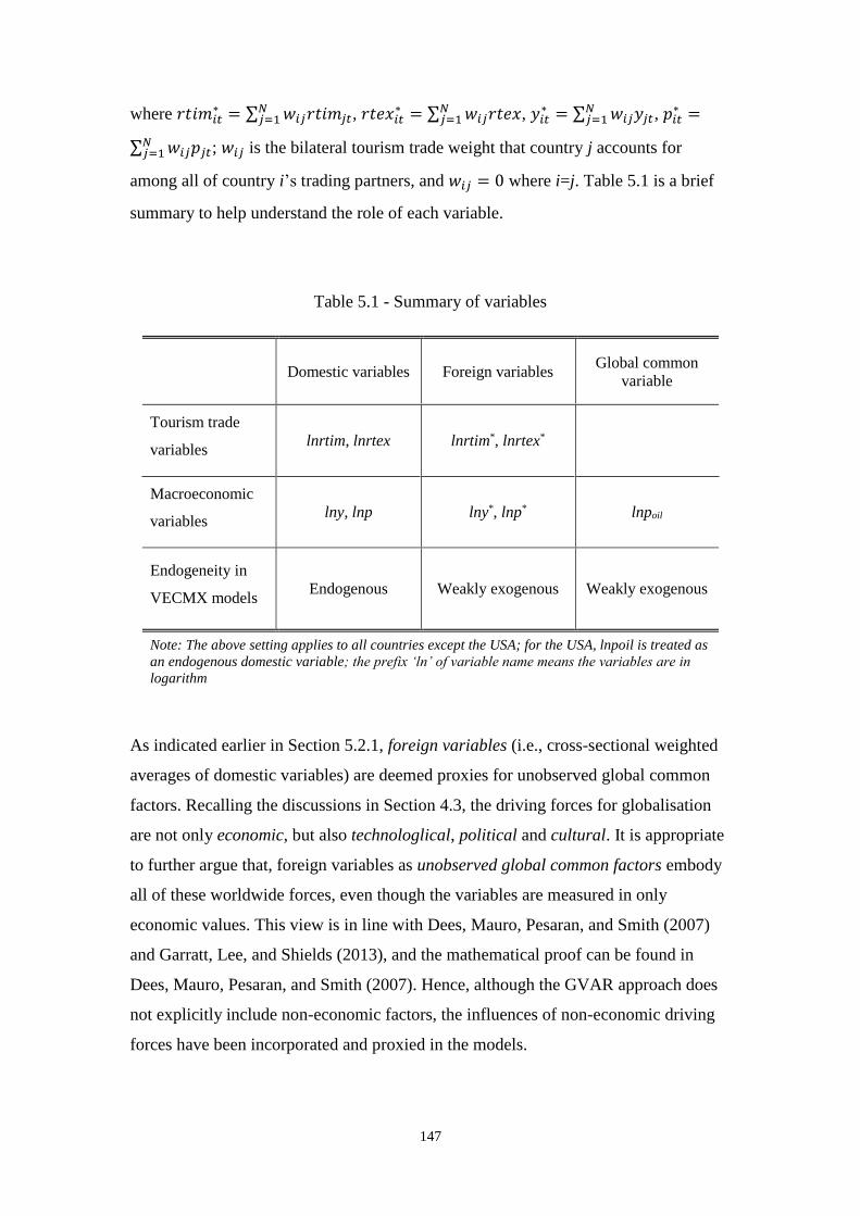
147
where 𝑟𝑡𝑖𝑚𝑖𝑡∗ = ∑ 𝑤𝑖𝑗𝑟𝑡𝑖𝑚𝑗𝑡
𝑁𝑗=1 , 𝑟𝑡𝑒𝑥𝑖𝑡
∗ = ∑ 𝑤𝑖𝑗𝑟𝑡𝑒𝑥𝑁𝑗=1 , 𝑦𝑖𝑡
∗ = ∑ 𝑤𝑖𝑗𝑦𝑗𝑡𝑁𝑗=1 , 𝑝𝑖𝑡
∗ =
∑ 𝑤𝑖𝑗𝑝𝑗𝑡𝑁𝑗=1 ; 𝑤𝑖𝑗 is the bilateral tourism trade weight that country j accounts for
among all of country i’s trading partners, and 𝑤𝑖𝑗 = 0 where i=j. Table 5.1 is a brief
summary to help understand the role of each variable.
Table 5.1 - Summary of variables
Domestic variables Foreign variables Global common
variable
Tourism trade
variables lnrtim, lnrtex lnrtim*, lnrtex*
Macroeconomic
variables lny, lnp lny*, lnp* lnpoil
Endogeneity in
VECMX models Endogenous Weakly exogenous Weakly exogenous
Note: The above setting applies to all countries except the USA; for the USA, lnpoil is treated as
an endogenous domestic variable; the prefix ‘ln’ of variable name means the variables are in
logarithm
As indicated earlier in Section 5.2.1, foreign variables (i.e., cross-sectional weighted
averages of domestic variables) are deemed proxies for unobserved global common
factors. Recalling the discussions in Section 4.3, the driving forces for globalisation
are not only economic, but also technologlical, political and cultural. It is appropriate
to further argue that, foreign variables as unobserved global common factors embody
all of these worldwide forces, even though the variables are measured in only
economic values. This view is in line with Dees, Mauro, Pesaran, and Smith (2007)
and Garratt, Lee, and Shields (2013), and the mathematical proof can be found in
Dees, Mauro, Pesaran, and Smith (2007). Hence, although the GVAR approach does
not explicitly include non-economic factors, the influences of non-economic driving
forces have been incorporated and proxied in the models.
148
That said, the foreign variables only embody the unobserved global common factors.
Any country-specific non-economic factors are still left out under the GVAR
framework. It should be noted that non-economic factors are difficult to properly
quantify. Simply adding unjustified and unappropriately measured non-economic
factors does not help to improve the econometric model’s explanatory power.
For all the countries that are covered in the current research, the same sets of
domestic, foreign and global variables are constructed. The only exception is the
USA’s VARX* model, which is regarded as a reference country in the global
economy (see Dees, Mauro, Pesaran, & Smith, 2007; Greenwood‐Nimmo, Nguyen, &
Shin, 2012). Its domestic variables and the foreign variables are:
𝒙𝑈𝑆𝐴,𝑡 = (𝑟𝑡𝑖𝑚𝑈𝑆𝐴,𝑡, 𝑟𝑡𝑒𝑥𝑈𝑆𝐴,𝑡, 𝑦𝑈𝑆𝐴,𝑡, 𝑝𝑈𝑆𝐴,𝑡, 𝑝𝑜𝑖𝑙𝑡) and
𝒙𝑖𝑡∗ = (𝑟𝑡𝑖𝑚𝑈𝑆𝐴,𝑡
∗ , 𝑟𝑡𝑒𝑥𝑈𝑆𝐴,𝑡∗ , 𝑦𝑈𝑆𝐴,𝑡
∗ , 𝑝𝑈𝑆𝐴,𝑡∗ ).
The difference is that, the oil price 𝑝𝑜𝑖𝑙𝑡 is deemed as an endogenous variable for the
USA. As hinted in Section 4.5.1, where the assumption of small economies is
discussed, the USA exerts more power in dominating the global economic and
political landscape than other countries. Since oil price is very sensitive, treating it as
an endogenous variable in the USA’s model allows the evolution of the global macro-
economic variables (in the form of USA’s foreign variables) to influence oil prices
(Dees, Mauro, Pesaran, & Smith, 2007) and captures the power of the USA on global
affairs. The appropriateness of treating the USA as a reference country is discussed in
great details in Chudik and Smith (2013).
For any other countries that will be sampled in the current research, none of them is as
powerful as the USA from the economic perspective. A brief evidence is the
prevalence of the US dollar in international markets. The dollar is the standard unit of
currency in goods, services and commodities trading. It is also the preferred reserve
currency for central banks as well as private holdings. The monetary policy by the
Federal Reserve Bank is closely eyed upon by other central banks (especially those
that operate a pegged exchange rate system against the dollar), due to the policy’s
implications on not only the interest rates and inflation rate in the USA, but also
potential impacts on other countries. As a result, in the current research, only the USA
is chosen as the reference country.
149
Country-Specific Model: VECMX
Following Bussière, Chudik, and Sestieri (2009) and Dees, Mauro, Pesaran, and
Smith (2007), the first stage country-specific VARX* models take the error correction
form augmented with exogenous variables, i.e., VECMX, which is written in reduced
form1 as:
∆𝒙𝑖𝑡 = 𝒂𝑖0 − 𝜶𝑖𝜷𝑖′[𝒛𝑖,𝑡−1 − 𝜸𝑖(𝑡 − 1)]
+𝚲𝑖0∆𝒙𝑖𝑡∗ + 𝚼𝑖0Δ𝒅𝑡 +𝚽𝑖(𝐿, 𝑝𝑖, 𝑞𝑖)∆𝒛𝑖,𝑡−1 + 𝒖𝑖𝑡 (5.8)
where 𝒛𝑖𝑡 = (𝒙𝑖𝑡′ , 𝒙𝑖𝑡
∗′ , 𝒅𝑡′)′; 𝜷𝑖 is the (𝑘𝑖 + 𝑘𝑖
∗ + 𝑘𝑑) × 𝑟𝑖 matrix denoting the long-run
cointegrating relationship between variables; 𝜶𝑖 is the 𝑘𝑖 × 𝑟𝑖 matrix of adjustment
coefficients measuring the speed of adjustment to long-run cointegration; 𝑝𝑖 and 𝑞
𝑖 are
the lag orders of the domestic variables 𝒙𝑖𝑡 and the other variables 𝒙𝑖𝑡∗ and 𝒅𝑡; 𝒂𝑖0, 𝜸𝑖,
𝚲𝑖0, 𝚼𝑖0 and 𝚽𝑖(𝐿, 𝑝𝑖 , 𝑞𝑖) are the parameters to be estimated. Determination of 𝜶𝑖 and
𝜷𝑖 can be based on the identity matrix normalisation scheme as described in Section
3.2.2.1.
The key parameters that capture the magnitude of interdependencies are matrix 𝜦𝑖0,
which constitute the factor loadings on ∆𝒙𝑖𝑡∗ . 𝚲𝑖0 denote the contemporaneous effects
of foreign variables on their domestic counterparts, for example, the percentage
change of a particular country’s tourism exports (rtex) in response to 1 percent change
of other countries’ tourism exports (rtex*).
The global VAR (GVAR) model is derived after estimating Eq. (5.8), following the
transformation procedure from Eq. (5.3) to Eq. (5.5).
Unit Root Tests
For the error correction form of VAR model (i.e., VECM), it is generally required that
the cointegration exists only between I(1) series. However, in practice this assumption
is not always strictly followed. The GVAR modelling, especially in its first stage (i.e.,
country-specific VECMX), can well accommodate both I(0) and I(1) series in the
1 Generally, VAR model written as 𝐵0𝑦𝑡 = 𝑐0 + 𝐵1𝑦𝑡−1 + 𝐵2𝑦𝑡−2 +⋯+ 𝐵𝑝𝑦𝑡−𝑝 + 𝜖𝑡 is denoted a
structural VAR (SVAR) with p lags. After pre-multiplying the SVAR with the inverse of 𝐵0, the SVAR
can be written in the reduced form as 𝑦𝑡 = 𝑐 + 𝐴1𝑦𝑡−1 + 𝐴2𝑦𝑡−2 +⋯+ 𝐴𝑝𝑦𝑡−𝑝 + 𝑒𝑡, where 𝑐 =
𝐵0−1𝑐0, 𝐴𝑖 = 𝐵0
−1𝐵𝑖 𝑓𝑜𝑟𝑖 = 1, 2… , 𝑝, and 𝑒𝑡 = 𝐵0−1𝜖0.
150
system (e.g., Assenmacher, 2013; Dees, Mauro, Pesaran, & Smith, 2007). As long as
a reduced rank of the coefficient matrix 𝚷 = 𝜶𝜷′, i.e., rank(𝚷) = r (0<r<k) in Eq.
(3.14), is detected, r cointegrating relations can be established.
The most commonly used unit root test is the augmented Dickey-Fuller (ADF) test,
which is based on
∆𝑦𝑡 = 𝛼𝑦𝑡−1 + 𝑥𝑡′𝛿 + ∑ 𝛽𝑗Δ𝑦𝑡−𝑗
𝑝𝑗=1 + 𝜈𝑡 (5.9)
where 𝑦𝑡 is the series in concern, 𝑥𝑡 is a vector of optional exogenous regressors, p is
the lag length of the differenced terms and can be decided using the information
criteria such as AIC and SBC, 𝛼, 𝛿 and 𝛽𝑗 (𝑗 = 1,2, … , 𝑝) are the coefficients to be
estimated. The unit root test is to test the null hypothesis 𝐻0: 𝛼 = 0 against the one-
sided alternative 𝐻1: 𝛼 < 0. If the null hypothesis is accepted, then it is found that the
series 𝑦𝑡 has a unit root. Otherwise, 𝑦𝑡 is said to be stationary.
While testing unit roots with the above ADF test is very much a standard practice in
empirical time series analysis, modifications of ADF test as well as alternative tests
are also often considered by researchers. Among others, the weighted symmetric
versions of ADF (WS-ADF) have been recognised as more powerful than the standard
ADF test (Dees, Mauro, Pesaran, & Smith, 2007; Patterson & Heravi, 2003) and been
applied in macroeconometric studies such as Galesi and Lombardi (2009).
Lag Orders (pi, qi) Selection
In Eq. (5.8), the lag order of the domestic variables, i.e., 𝑝𝑖, and that of the foreign and
global common variables, i.e., 𝑞𝑖, can be selected based on the Akaike information
criterion (AIC) or the Schwarz Bayesian criterion (SBC). These are computed as
follows:
Akaike information criterion (AIC):
𝐴𝐼𝐶𝑖,𝑝𝑞 = −𝑇𝑘𝑖
2(1 + 𝑙𝑜𝑔2𝜋) −
𝑇
2log|Σ̂𝑖| − 𝑘𝑖𝑠𝑖 (5.10)
Schwarz Bayesian criterion (SBC):
𝑆𝐵𝐶𝑖,𝑝𝑞 = −𝑇𝑘𝑖
2(1 + 𝑙𝑜𝑔2𝜋) −
𝑇
2log|Σ̂𝑖| −
𝑘𝑖𝑠𝑖
2𝑙𝑛𝑇 (5.11)

151
where Σ̂𝑖 = ∑ �̂�𝑖𝑡�̂�′𝑖𝑡′/𝑇
𝑇𝑡=1 and �̂�𝑖𝑡 are the estimated residuals obtained from Eq.
(5.8), T is the sample size, |Σ̂𝑖| is the determinant of Σ̂𝑖, 𝑘𝑖 is the number of domestic
variables (𝑘𝑖 becomes 𝑘𝑖∗ in the case of foreign variables), and 𝑠𝑖 = 𝑘𝑖𝑝𝑖 + 𝑘𝑖
∗𝑞𝑖 + 2.
The model with the highest AIC or SBC value is chosen.
It should, however, be noted that 𝑝𝑖 and 𝑞𝑖 need not be the same across different
country-specific models, i.e., Eq. (5.8). Following Dees, Mauro, Pesaran, and Smith
(2007), the lag orders is allowed to be set arbitrarily in case of data limitations (e.g.,
low order for relatively small sample size).
Deterministics of the VECMX Model
As reviewed in Section 3.2.2.1, the estimation of a VEC model involves whether or
not to restrict the deterministic components, i.e., the intercepts and the trend terms, in
the cointegrating vectors. Five cases have been discussed in Section 3.2.2.1.
Generally, Case III and Case IV are considered particularly relevant to
macroeconomic analysis (Garratt, Lee, Pesaran, & Shin, 2012, p.122; Song, Witt, &
Li, 2009, p.130), even though the preference between Case III and Case IV differs
from one research area to another.
Case III: unrestricted intercepts and no trend coefficients
Case IV: unrestricted intercepts and restricted trend coefficients
Since the intercepts in both the above cases are unrestricted and the trend term (only
exists in Case IV) is restricted to the cointegration space, it means that the level of the
endogenous variables contains a linear, but not quadratic, trend1. For modelling
purposes, the current research sets the deterministics of the VECMX model to Case
IV, so as to allow for trends in the long-run equilibrium of an economy.
Rank Orders (ri): Number of Cointegrating relations
1 Since the dependent variables in the VEC model are differenced terms and are in logarithm, an
intercept is equivalent to a constant growth for the level of the variables. Hence, the level of the
variables has a linear trend.

152
As set out in Section 2.2.2.1, the number of cointegrating relations in a VECMX
model can be determined following the Johansen maximum likelihood (JML)
approach.
Two types of log-likelihood ratio statistics can be derived using Eq. (3.15), i.e.,
𝜆𝑡𝑟𝑎𝑐𝑒 = −𝑇∑ ln(1 − �̂�𝑖)𝑚𝑖=𝑟+1 , and Eq. (3.16), i.e., 𝜆𝑚𝑎𝑥 = −𝑇ln(1 − �̂�𝑟+1). The
null hypothesis for both tests is H0: rank(𝚷) = r, meaning there are r cointegrating
relations. The trace statistics is intended for testing the null hypothesis against the full
rank hypothesis, H1: rank(𝚷) = m. The maximum eigenvalue statistics is intended for
testing the null hypothesis against the null against H1: rank(𝚷) = r + 1 (Garratt, Lee,
Pesaran, & Shin, 2012, p.123). The critical values for VEC models containing
exogenous I(1) variables have been reported by Pesaran, Shin, and Smith (2000)
across Case I to Case V. In the case of a small sample size, it is suggested that the
trace statistics can yield better power than the maximal eigenvalue statistics (Dees,
Mauro, Pesaran, & Smith, 2007), and hence the determination of r in the current
research primarily relies on the trace statistics. It is, however, allowed that r can be
adjusted after preliminary estimation of the VECMX model, in order to yield better
estimation results. For example, reducing r (that is less cointegrating relations) to
obtain more stable persistence profiles. It is also suggested by Juselius (2006, pp.140-
142) that the choice of rank orders is not only a statistical process, but is also based on
the economic interpretability of the results.
Weak Exogeneity Test
One of the major assumptions underlying the country-specific VECMX model is the
weak exogeneity of the foreign variables 𝒙𝑖𝑡∗ and the global variables 𝒅𝑡. A formal test
for weak exogeneity can be performed via auxiliary equations for the foreign
variables, as outlined by Dees, Mauro, Pesaran, and Smith (2007).
Specifically, for each lth element of 𝒙𝑖𝑡∗ , the following regression is carried out:
∆𝒙𝑖𝑡,𝑙∗ = 𝝁𝑖𝑙 +∑ 𝜸𝑖𝑗,𝑙𝑬𝑪𝑴𝑖,𝑡−1
𝑗𝑟𝑖
𝑗=1+∑ 𝝋𝑖𝑘,𝑙∆𝒙𝑖,𝑡−𝑘
𝑠𝑖
𝑘=1+
∑ 𝝑𝑖𝑚,𝑙∆�̃�𝑖,𝑡−𝑚∗𝑛𝑖
𝑚=1 + 𝜺𝑖𝑡,𝑙 (5.12)

153
where 𝐸𝐶𝑀𝑖,𝑡−1𝑗
, j = 1, 2, …, ri are the estimated error correction terms corresponding
to the ri cointegrating relations found for the ith country model and Δ�̃�𝑖,𝑡∗ =
(Δ𝒙′𝑖𝑡∗ , Δ𝑝𝑜𝑖𝑙𝑡)′. The lag orders 𝑠𝑖 and 𝑛𝑖 in Eq. (5.12) need not be the same as the
orders pi and qi of the underlying country-specific VECMX models. Hence, Eq. (5.12)
is seen independent of Eq. (5.8). The test for weak exogeneity is an F-test of the joint
hypothesis that 𝛾𝑖𝑗,𝑙 = 0, j = 1, 2, …, ri in Eq. (5.12). Passing the weak exogeneity test
means the error correction mechanism does not exist for 𝒙𝑖𝑡∗ to restore the long-run
equilibrium. Hence, there is no ‘long-run forcing’ from 𝒙𝑖𝑡 to 𝒙𝑖𝑡∗ , but only short-run
feedbacks for 𝒙𝑖𝑡∗ .
Persistence Profiles
Persistence profiles (PPs) refer to the time profile of the effects of system-wide or
variable-specific shocks on cointegrating relations in the context of VAR models
(Pesaran & Shin, 1996). They measure the speed with which an economy returns its
long-run equilibrium, once shocked. In the case of relations between I(1) variables
that are not cointegrated, the effect of a shock persists forever, while in the case of
cointegrated relations the impact of a shock will be transitory and eventually
disappear as the economy restores equilibrium (Pesaran & Shin, 1996). PPs are scaled
to a value of unity on the initial impact, while they should tend to zero as the horizon
𝑛 → ∞, if the cointegration vector is valid.
Consider Eq. (5.7), and for simplicity treat the global common variable 𝒅𝑡 as an
element in 𝒙𝑡, such that the reduced form GVAR becomes 𝒙𝑡 = 𝒃0 + 𝒃1𝑡 +
∑ 𝑭𝑗𝒙𝑡−𝑗𝑝𝑗=1 + 𝜺𝑡. Its moving average representation is given by
𝒙𝑡 = 𝒃0 + 𝒃1𝑡 + ∑ 𝑨𝑠𝜺𝑡−𝑠∞𝑠=1 (5.13)
where each 𝑨𝑠 itself can be derived recursively as
𝑨𝑠 = 𝑭1𝑨𝑠−1 + 𝑭2𝑨𝑠−2 +⋯+ 𝑭𝑝𝑨𝑠−𝑝, for s=1, 2, … (5.14)
wtih 𝑨0 = 𝑰𝑘, 𝑨𝑠 = 𝟎 for any s<0.

154
Let 𝒛𝑖𝑡 = (𝒙𝑖𝑡′ , 𝒙𝑖𝑡
∗′)′ (same as in Eq. (5.8), but treat 𝒅𝑡 as part of 𝒙𝑖𝑡∗ only for
simplicity). Let 𝑽𝑖 = (𝑬𝑖,𝑾𝑖)′. 𝑬𝑖 and 𝑾𝑖 are defined in Eq. (5.3). Since 𝒙𝑖𝑡 = 𝑬𝑖′𝒙𝑡
and 𝒙𝑖𝑡∗ = 𝑾𝑖
′𝒙𝑡, thus
𝒛𝑖𝑡 = (𝒙𝑖𝑡′ , 𝒙𝑖𝑡
∗′)′ = 𝑽𝑖𝒙𝑡 (5.15)
Eq. (5.15) provides the mapping between 𝒛𝑖𝑡 and 𝒙𝑡.
Since the cointegrating relations for any specific country (as in Eq. (5.8)) are given in
terms of the country-specific domestic and foreign variables, in the form of 𝜷𝑖′𝒛𝑖𝑡 (as
in Eq. (5.8)). From Eq. (5.13), it can be derived that
𝒛𝑖𝑡 = 𝑽𝑖(𝒃0 + 𝒃1𝑡) + 𝑽𝑖 ∑ 𝑨𝑠𝜺𝑡−𝑠∞𝑠=1 (5.16)
The PPs of 𝜷𝑗𝑖′ 𝒛𝑖𝑡, with respect to a system-wide shock to 𝜺𝑡, are
ΡΡ(𝜷𝑗𝑖′ 𝒛𝑖𝑡; 𝜺𝑡, 𝑛) =
𝜷𝑗𝑖′ 𝑽𝑖𝑨𝑛𝚺𝜀𝑨𝑛
′ 𝑽𝑖′𝜷𝑗𝑖
𝜷𝑗𝑖′ 𝑽𝑖𝑨0𝚺𝜀𝑨0
′𝑽𝑖′𝜷𝑗𝑖
, n = 0, 1, 2, … (5.17)
where 𝜷𝑗𝑖′ is the jth cointegrating relation in the ith country (j=1, 2, …, ri), n is the
horizon and 𝚺𝜀 is the covariance matrix of 𝜺𝑡.
5.2.3 Impulse Response Analysis
One important use of macroeconometric models is to conduct counterfactual
experiments in order to interpret previous historical episodes and to help with policy
analysis. For example, an analysis of the dynamic impact of shocks is typically carried
out using impulse response functions that focus on the evolution of the conditional
means of the target variables in response to different types of shocks. (Garratt, Lee,
Pesaran, & Shin, 2012, p.225). Here, counterfactual experiments are posed by ‘what
if’ questions, and are considered in decision making under uncertainty in relation to
hypothetical states of the world (Pesaran & Smith, 2012). It is worth reiterating that,
in economics a shock refers to an unexpected or unpredictable event that affects an
economy either positively or negatively. Technically in econometrics, the
unpredictable change takes place in exogenous factors, which are not explained by the
endogenous variables in the model.
Impulse response analysis is intended to characterise the evolution of a system at
different future periods in response to the effect of shocking one of the variables

155
within the system (Pesaran, Schuermann, & Weiner, 2004). With the moving average
representation of a VAR model, e.g., Eq. (5.13), one can derive the impulse responses
of the endogenous variables to a ‘unit’ displacement in the particular elements of
either the exogenous variables (if any) or the errors. The former represent the time
profile of the response of the system to changes in the observed forcing variables of
the system, while the latter examine the responses of the system to changes in the
unobserved forcing variables (Garratt, Lee, Pesaran, & Shin, 2012, pp.111-112).
In the current research, the counterfactual experiments are scenarios related to
unexpected changes of the Chinese economy. Specifically, it is presumed that the
Chinese economy experienced a sudden slowdown in its real GDP; another
presumption is that the Chinese currency experienced a depreciation, and as a result a
slump in its own price. Accordingly in the GVAR model, two individual shocks are to
be imposed: a negative shock to China’s real GDP variable (lny) and a negative shock
to China’s own price variable (lnp).
These two counterfactual scenarios have their practical grounding, as discussed in
Section 4.6.2. China’s GDP growth has been relaxed in the very recent years. A
negative shock to China’s GDP, equivalent to a sudden recession, is indeed a strong
presumption given that in reality China is still expecting economic growth. Defining
this counterfactual scenario is to test how ‘devastating’ (if any) the world tourism
market could become in a dire situation. The other shock, to China’s own price, is
more in accordance with the recent speculation that China would devaluate its
currency. The event itself (if realised) is not necessarily an adverse situation for other
countries.
It is proposed by Pesaran, Schuermann, and Weiner (2004) to make use of the
generalised impulse response (GIR) functions, instead of the traditionally used
orthogonalised impulse response (OIR) functions. In the context of the global VAR
(GVAR) approach, OIR depends on the order of factors in each country and on the
order in which the countries are stacked in xt, whereas the GIR function is invariant to
the ordering (Dees, Mauro, Pesaran, & Smith, 2007; Pesaran, Schuermann, & Weiner,
2004). Hence, the current research adopts the generalised impulse response analysis.

156
The derivation of GIR functions follows a similar process to the persistence profiles.
Consider the GVAR model Eq. (5.5), and for simplicity the lag orders are set to be 1.
Then Eq. (5.5) can be re-written as follows:
𝑮0𝒙𝑡 = 𝒂0 + 𝒂1𝑡 + 𝑮1𝒙𝑡−1 + 𝚼0𝒅𝑡 + 𝚼1𝒅𝑡−1 + 𝒖𝑡 (5.18)
Assuming 𝑮0 is nonsingular, the reduced-form global model can be obtained as
𝒙𝑡 = 𝒃0 + 𝒃1𝑡 + 𝑭𝒙𝑡−1 + 𝚪0𝒅𝑡 + 𝚪1𝒅𝑡−1 + 𝜺𝑡 (5.19)
where 𝒃0 = 𝑮0−1𝒂0, 𝒃1 = 𝑮0
−1𝒂1, 𝑭 = 𝑮0−1𝑮1, 𝚪0 = 𝑮0
−1𝚼0, 𝚪1 = 𝑮0−1𝚼1, and 𝜺𝑡 =
𝑮0−1𝒖𝑡.
For predetermined values of 𝒅𝑡 (t = T+1, T+2 …), it can be solved based on Eq. (5.19)
that
𝒙𝑇+𝑛 = 𝑭𝑛𝒙𝑇 +∑ 𝑭𝜏[𝒃0 + 𝒃1(𝑇 + 𝑛 − 𝜏)]𝑛−1
𝜏=0
+∑ 𝑭𝜏[𝚪0𝒅𝑇+𝑛−𝜏 + 𝚪1𝒅𝑇+𝑛−𝜏−1]𝑛−1𝜏=0
+∑ 𝑭𝜏𝜺𝑇+𝑛−𝜏𝑛−1𝜏=0 (5.20)
The point forecasts of 𝒙𝑇+𝑛 conditional on the initial state of the system and the
exogenous global variables are given by
𝒙𝑇+𝑛𝑓
= 𝐸(𝒙𝑇+𝑛|𝒙𝑇 , ⋃ 𝒅𝑇+𝜏𝑛𝜏=1 )
= 𝑭𝑛𝒙𝑇 + ∑ 𝑭𝜏[𝒃0 + 𝒃1(𝑇 + 𝑛 − 𝜏)]𝑛−1𝜏=0
+∑ 𝑭𝜏[𝚪0𝒅𝑇+𝑛−𝜏 + 𝚪1𝒅𝑇+𝑛−𝜏−1]𝑛−1𝜏=0 (5.21)
Under the assumption that 𝒖𝑡 (as in Eq. (5.18)) is normally distributed, it follows that
𝒙𝑇+𝑛|𝒙𝑇 , ⋃ 𝒅𝑇+𝜏𝑛𝜏=1 ∽ 𝑁(𝒙𝑇+𝑛
𝑓, 𝛀𝑛) (5.22)
where 𝛀𝑛 = ∑ 𝑭𝜏𝑮0−1𝚺𝑮0
′−1𝑭′𝜏𝑛−1𝜏=0 , 𝚺 is the 𝑘 × 𝑘 variance-covariance matrix of the
shocks 𝒖𝑡, which is the same as in Eq. (5.1). 𝚺𝑖𝑗, which measures the dependence of
shocks in country i on the shocks in country j, is defined as 𝚺𝑖𝑗 = 𝑐𝑜𝑣(𝒖𝑖𝑡, 𝒖𝑗𝑡). A
typical element of 𝚺𝑖𝑗 is denoted by 𝜎𝑖𝑗,𝑙𝑠 = 𝑐𝑜𝑣(𝑢𝑖𝑙𝑡, 𝑢𝑗𝑠𝑡), which is the covariance of
the lth variable in country i with the sth variable in country j.

157
With the above in mind, it follows Pesaran, Schuermann, and Weiner (2004) that the
GIR function which denotes the jth shock in 𝒖𝑡 (corresponding to the lth variable in the
ith country), is given by:
𝑮𝑰𝑥:𝑢𝑖𝑙(𝑛,√𝜎𝑖𝑖,𝑙𝑙 , ℐ𝑡−1) = 𝐸(𝒙𝑡+𝑛|𝑢𝑖𝑙𝑡 = √𝜎𝑖𝑖,𝑙𝑙, ℐ𝑡−1) − 𝐸(𝒙𝑡+𝑛|ℐ𝑡−1) (5.23)
where 𝓘𝑡 = (𝒙𝑡, 𝒙𝑡−1, … ) is the information set at time t - 1 and dt is assumed to be
given exogenously. On the assumption that ut has a multivariate normal distribution,
and using Eq. (5.20), it is derived that
𝝍𝑗𝑔(𝑛) =
1
√𝜎𝑖𝑖,𝑙𝑙𝑭𝑛𝑮0
−1𝚺𝜻𝑗 (5.24)
where 𝜻𝑗 is a 𝑘 × 1 selection vector with unity as its jth element (corresponding to a
particular shock in a particular country) and zeros elsewhere. Eq. (5.24) measures the
effect of one standard error shock to the jth equation (corresponding to the lth variable
in the ith country) at time t on the expected values of x at time t + n.
5.3 Data Descriptions
The data that are required to model the interdependencies of tourism demand are
described in Section 5.2.2. They mostly can be obtained from major macroeconomic
databases, even though it is unavoidable that the availability of data varies from one
database to another. If the data of all domestic variables across countries are arranged
as panel data, it is rare that the data set will be a balanced one, due to the missing
observations of certain variables for certain countries and at certain quarters/years.
Building a data set for the GVAR analysis hence involves a careful trade-off between
the number of countries under consideration and the length of sample period.
Wherever necessary, interpolation of missing data have to be applied.
5.3.1 Data Sources
The current research takes into consideration 24 major countries across the globe.
They are shown in Table 5.2. While the more countries included in the global VAR
(GVAR) model, the more complete the study can be, the final choice of the countries
to be analysed is down to several concerns.
The first is data availability. Measures of tourism demand in the current research are
tourism imports and tourism exports. But tourism trade figures are not as widely

158
reported as other tourism demand measures (e.g., tourism arrivals). Besides, the
desirable frequency of data is quarterly/monthly, so as to generate more observations
over a defined sample period. But quarterly data are less commonly seen than annual
data. Eventually, the raw data have been gathered from several sources, as listed in
Table 5.3. It should be reiterated that for tourism imports and tourism exports, the data
contain travel items and passenger transport items from the Balance of Payments data
published by IMF. The use of BOP data is in line with the World Travel & Tourism
Council’s practice and the BOP data are acknowledged to be consistent with
UNWTO’s data on tourism expenditure and receipts (see Section 3.2, and see WTTC,
2015, p.11). The availability of as many data and as many quarters covered as
possible primarily dictates which countries to include. The second is a country’s
importance in the world tourism market. Top tourism destinations/origins are hence
preferred. To this end, the statistics on international tourist arrivals and international
tourism receipts from Tourism Highlights (UNWTO, 2013, 2014a, 2015) have been
used for reference. According to Table 5.4 and Table 5.5, the 24 countries under
consideration constantly accounted for over half of the world’s tourism market (about
55% of the international arrivals, 61% of the tourism receipts), and they are all among
the top destinations within their home continent. In addition, Australia, Brazil,
Canada, China, France, Germany, Italy, Japan, UK and USA have constantly or
recently made the list of top ten spenders in international tourism (see Table 1.4). So it
is expected that the 24 countries listed in Table 5.2 can well represent the world
tourism market to a large extent. The third is global coverage. As the GVAR model
concerns the linkages between countries on a global scale, it is desirable to include
countries from as many continents as possible, rather than only from one continent or
two.
Ideally, all the rest of the countries in the world can be aggregated to form an
imagined country called ‘Rest of the World (ROW)’ and be included in the GVAR
analysis. The construction of this ROW country is however hindered by the limited
availability of data, with rampant missing values across countries over the sample
period. Nevertheless, the GVAR model can still work fairly well without aggregating
the rest in the system (see for example, Chudik & Fratzscher, 2011; Dees, Mauro,
Pesaran, & Smith, 2007; Koukouritakis, Papadopoulos, & Yannopoulos, 2015;
Pesaran, Schuermann, & Weiner, 2004).
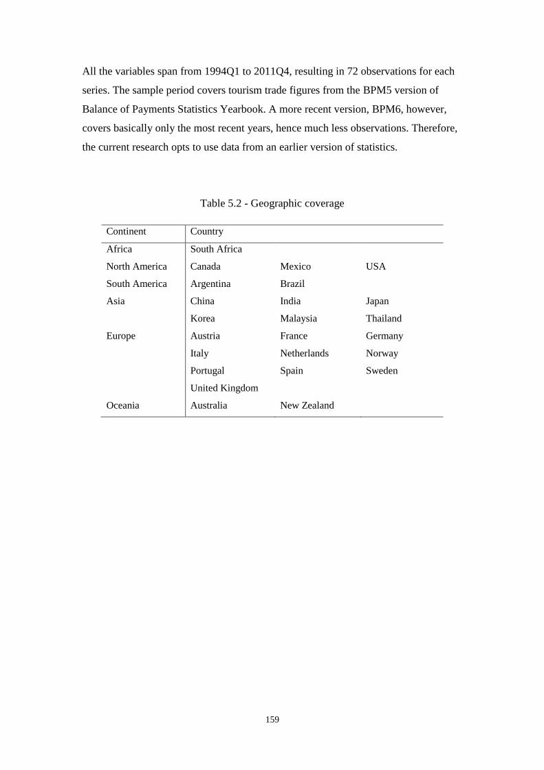
159
All the variables span from 1994Q1 to 2011Q4, resulting in 72 observations for each
series. The sample period covers tourism trade figures from the BPM5 version of
Balance of Payments Statistics Yearbook. A more recent version, BPM6, however,
covers basically only the most recent years, hence much less observations. Therefore,
the current research opts to use data from an earlier version of statistics.
Table 5.2 - Geographic coverage
Continent Country
Africa South Africa
North America Canada Mexico USA
South America Argentina Brazil
Asia China India Japan
Korea Malaysia Thailand
Europe Austria France Germany
Italy Netherlands Norway
Portugal Spain Sweden
United Kingdom
Oceania Australia New Zealand

160
Table 5.3 - Summary of data sources
Variable Measure Frequency Source
Nominal tourism
imports
Travel debits (million US$);
passenger transport debits
(million US$)
Quarterly Balance of Payments
Statistics Yearbook
(BPM5), IMF
Nominal tourism
exports
Travel credits (million US$);
passenger transport credits
(million US$)
Quarterly Balance of Payments
Statistics Yearbook
(BPM5), IMF
Income level Real GDP index (year 2005
= 100)
Quarterly International Financial
Statistics, IMF; national
statistical office
Consumer prices CPI (year 2005 = 100) Quarterly International Financial
Statistics, IMF; main
economic indicators,
OECD
Exchange rates National currency against US
dollar
Quarterly International Financial
Statistics, IMF
Oil prices Petroleum: average crude
price (US$ per barrel)
Quarterly International Financial
Statistics, IMF
Bilateral trade volume Average of exports and
imports (in US$)
Annual Direction of Trade
Statistics, IMF
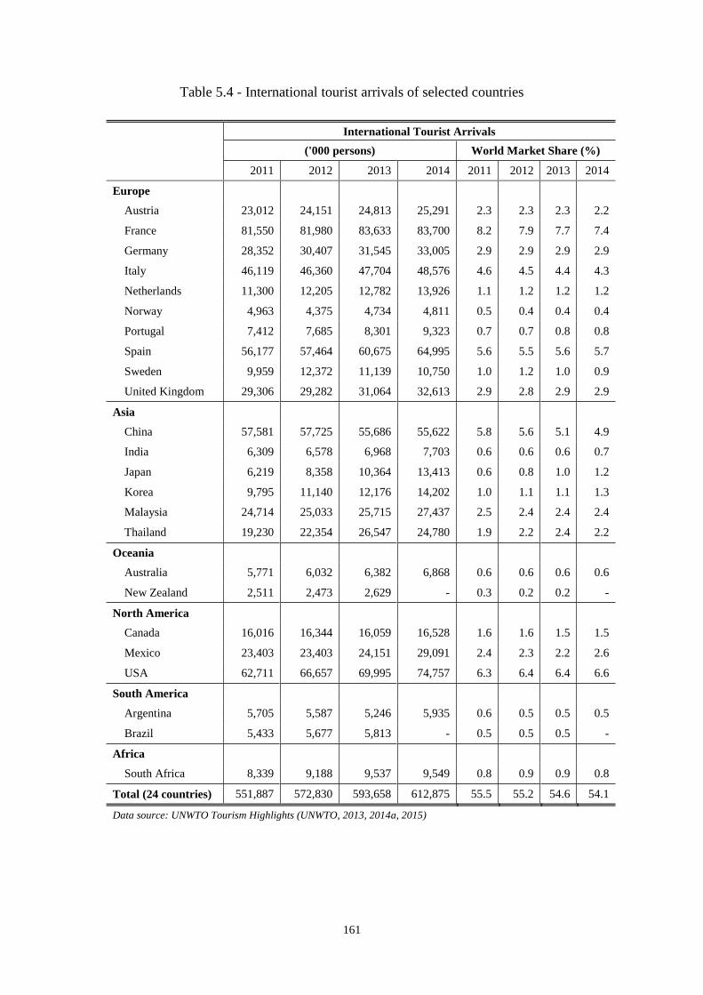
161
Table 5.4 - International tourist arrivals of selected countries
International Tourist Arrivals
('000 persons) World Market Share (%)
2011 2012 2013 2014 2011 2012 2013 2014
Europe
Austria 23,012 24,151 24,813 25,291 2.3 2.3 2.3 2.2
France 81,550 81,980 83,633 83,700 8.2 7.9 7.7 7.4
Germany 28,352 30,407 31,545 33,005 2.9 2.9 2.9 2.9
Italy 46,119 46,360 47,704 48,576 4.6 4.5 4.4 4.3
Netherlands 11,300 12,205 12,782 13,926 1.1 1.2 1.2 1.2
Norway 4,963 4,375 4,734 4,811 0.5 0.4 0.4 0.4
Portugal 7,412 7,685 8,301 9,323 0.7 0.7 0.8 0.8
Spain 56,177 57,464 60,675 64,995 5.6 5.5 5.6 5.7
Sweden 9,959 12,372 11,139 10,750 1.0 1.2 1.0 0.9
United Kingdom 29,306 29,282 31,064 32,613 2.9 2.8 2.9 2.9
Asia
China 57,581 57,725 55,686 55,622 5.8 5.6 5.1 4.9
India 6,309 6,578 6,968 7,703 0.6 0.6 0.6 0.7
Japan 6,219 8,358 10,364 13,413 0.6 0.8 1.0 1.2
Korea 9,795 11,140 12,176 14,202 1.0 1.1 1.1 1.3
Malaysia 24,714 25,033 25,715 27,437 2.5 2.4 2.4 2.4
Thailand 19,230 22,354 26,547 24,780 1.9 2.2 2.4 2.2
Oceania
Australia 5,771 6,032 6,382 6,868 0.6 0.6 0.6 0.6
New Zealand 2,511 2,473 2,629 - 0.3 0.2 0.2 -
North America
Canada 16,016 16,344 16,059 16,528 1.6 1.6 1.5 1.5
Mexico 23,403 23,403 24,151 29,091 2.4 2.3 2.2 2.6
USA 62,711 66,657 69,995 74,757 6.3 6.4 6.4 6.6
South America
Argentina 5,705 5,587 5,246 5,935 0.6 0.5 0.5 0.5
Brazil 5,433 5,677 5,813 - 0.5 0.5 0.5 -
Africa
South Africa 8,339 9,188 9,537 9,549 0.8 0.9 0.9 0.8
Total (24 countries) 551,887 572,830 593,658 612,875 55.5 55.2 54.6 54.1
Data source: UNWTO Tourism Highlights (UNWTO, 2013, 2014a, 2015)

162
Table 5.5 - International tourism receipts of selected countries
International Tourism Receipts
(US$ million) World Market Share (%)
2011 2012 2013 2014 2011 2012 2013 2014
Europe
Austria 19,860 18,894 20,236 20,559 1.9 1.7 1.7 1.7
France 54,753 53,702 56,683 55,402 5.3 4.8 4.7 4.4
Germany 38,879 38,136 41,279 43,326 3.7 3.4 3.4 3.5
Italy 43,000 41,185 43,912 45,545 4.1 3.7 3.7 3.7
Netherlands 14,348 12,314 13,779 14,716 1.4 1.1 1.2 1.2
Norway 5,308 5,442 5,675 5,643 0.5 0.5 0.5 0.5
Portugal 11,339 11,056 12,284 13,808 1.1 1.0 1.0 1.1
Spain 60,031 58,162 62,565 65,187 5.8 5.2 5.2 5.2
Sweden 10,404 10,613 11,544 12,695 1.0 1.0 1.0 1.0
United Kingdom 35,069 36,613 41,028 45,262 3.4 3.3 3.4 3.6
Asia
China 48,464 50,028 51,664 56,913 4.7 4.5 4.3 4.6
India 17,707 17,971 18,397 19,700 1.7 1.6 1.5 1.6
Japan 10,966 14,576 15,131 18,853 1.1 1.3 1.3 1.5
Korea 12,476 13,429 14,629 18,147 1.2 1.2 1.2 1.5
Malaysia 19,656 20,250 21,496 21,820 1.9 1.8 1.8 1.8
Thailand 27,184 33,855 41,780 38,437 2.6 3.0 3.5 3.1
Oceania
Australia 31,335 31,898 31,254 32,022 3.0 2.9 2.6 2.6
New Zealand 7,341 7,128 7,472 8,464 0.7 0.6 0.6 0.7
North America
Canada 16,834 17,407 17,656 17,445 1.6 1.6 1.5 1.4
Mexico 11,869 12,739 13,949 16,258 1.1 1.1 1.2 1.3
USA 115,552 161,631 172,901 177,240 11.1 14.5 14.4 14.2
South America
Argentina 5,354 4,887 4,313 4,627 0.5 0.4 0.4 0.4
Brazil 6,555 6,645 6,704 6,843 0.6 0.6 0.6 0.5
Africa
South Africa 9,547 9,994 9,238 9,348 0.9 0.9 0.8 0.8
Total (24 countries) 633,831 688,555 735,569 768,260 60.8 61.7 61.4 61.7
Data source: UNWTO Tourism Highlights (UNWTO, 2013, 2014a, 2015)
163
5.3.2 Data Processing
As outlined in Section 5.2.2, the actual variables that enter the empirical model are
real tourism imports, real tourism exports, real income, own price (CPI adjusted by
exchange rate) and crude oil prices.
The variables of real tourism imports (rtim) and real tourism exports (rtex), as advised
by previous literature (e.g., Smeral, 2012; Smeral & Weber, 2000), are the tourism
imports and tourism exports in million US dollars at the prices and exchange rates of
the base year. These are each country’s total tourism imports from and total tourism
exports to all countries in the world, rather than the trades with other 23 countries
sampled in the current research. 2005 is chosen as the base year to yield real term
figures. The real income (y) variable is real GDP index adjusted to US dollar terms at
constant prices and exchange rates. The own price variable (p) is CPI data adjusted by
current exchange rate level (not constant exchange rates)1. Oil prices (poil) are
transformed to index. All the five variables are then taken logarithm.
However, there are several additional treatments to the data before fitting them into
the empirical models. These include seasonal adjustment, in order to remove the
seasonality in the data; interpolation of missing observations for certain variables. To
construct the foreign variables in the first stage VECMX models, bilateral trade
shares are used as weights.
Seasonal Adjustment
For quarterly or monthly economic data, such as retail sales, seasonal patterns can
generally be observed. For example, the volume of retail sales tends to rise during
December due to Christmas. This type of short-term phenomena, associated with the
time of the year, is seasonality, which may obscure or confound other underlying
movements of the data. The purpose of seasonal adjustment is to remove such
systematic effects and facilitates comparisons between consecutive time periods.
Time series are generally thought of as combinations of three basic components plus
irregular fluctuations (as introduced in Section 3.3.3). The three basic components are
1 Here, the own price variable is defined slightly different from that introducted in Section 2.4.4. It
involves only the exchange-rate-adjusted CPI of a specific countries, rather than a comparison of
exchange-rate-adjusted CPI between destination and origin.

164
seasonality, cycle and trend. Seasonality, as explained, is calendar related. Cycle is
regular or periodic fluctuations around the trend. Trend represents the medium- to
long-term direction of the series. Irregular fluctuations are usually due to certain
unpredictable factors, which affect the evolution of the time series on a random basis.
The rationale behind seasonal adjustment is thus to remove the seasonal component
from the time series.
For the current research, seasonal adjustment has been carried out on the raw data of
nominal tourism exports, nominal tourism imports, and real GDP index, as they
exhibit apparent seasonal patterns. This is done by using the X-13 ARIMA-SEATS
package available in EViews 8. The package is the latest version of the seasonal
adjustment tool developed by the U.S. Census Bureau.
Interpolation of Missing Data
The raw data of nominal tourism exports, nominal tourism imports and real GDP
index contain missing observations for some countries. To make the most of these
series, interpolation has been performed using the STAMP 7.10 package of
OxMetrics 4.1 software.
The model used by STAMP essentially follows the structural time series model
(STSM) and the basic structural model (BSM), as explained in Section 3.3.3 and
Section 3.3.4. So the model decomposes a time series into the seasonal, cycle, trend
and irregular components. The raw data are first fed into the model in order to obtain
satisfactory coefficients. The missing observations are then backcast based on the
estimated model.
Constructing Weight Matrices
As shown in Eq. (5.2), the foreign variables for the country-specific models are cross-
sectional weighted averages of domestic variables. A common weighting scheme is to
use the bilateral trade figures between countries. Table 5.6 and Table 5.7 illustrate the
calculation based on a small number of countries. Both are used as examples only.
Eight countries are chosen in the above example, namely Australia, Canada, China,
France, Germany, Japan, UK and USA. Each number represents the trading between
the column country and the row country, calculated as (𝑒𝑥𝑝𝑜𝑟𝑡𝑠 + 𝑖𝑚𝑝𝑜𝑟𝑡𝑠) 2⁄ . The

165
table is read from column to column. For example, column one (i.e., AUS) denotes
the trading relationship between Australia and the rest seven countries.
Table 5.6 - Country level bilateral trade
Based on Table 5.6, the share of each country in another country’s total trading is
calculated in Table 5.7. It should be noted that each column sums to one.
Table 5.7 - Country level trade shares
Hence, from the first column, among the total trading between Australia and the rest
seven countries, Canada accounts for roughly 1% (or 0.01), China 45% (or 0.45),
Unit: US$ billion
AUS CAN CHN FRA DEU JPN GBR USA
AUS 0.00 1.94 57.42 3.17 5.69 37.31 6.55 19.04
CAN 1.76 0.00 23.41 3.39 6.05 10.93 12.61 300.73
CHN 60.99 35.23 0.00 26.42 79.87 172.86 30.95 260.62
FRA 2.75 4.64 26.16 0.00 118.09 10.01 35.23 34.81
DEU 7.23 9.11 84.60 116.71 0.00 23.40 65.39 74.77
JPN 36.25 12.63 170.85 7.77 19.03 0.00 9.39 99.31
GBR 7.74 15.25 29.33 37.65 75.42 11.84 0.00 54.06
USA 19.82 289.66 222.01 26.97 60.85 101.97 45.32 0.00
Total 136.54 368.46 613.77 222.07 365.00 368.32 205.42 843.33
Source: Direction of Trade Statistics, IMF, 2011
AUS CAN CHN FRA DEU JPN GBR USA
AUS 0.00 0.01 0.09 0.01 0.02 0.10 0.03 0.02
CAN 0.01 0.00 0.04 0.02 0.02 0.03 0.06 0.36
CHN 0.45 0.10 0.00 0.12 0.22 0.47 0.15 0.31
FRA 0.02 0.01 0.04 0.00 0.32 0.03 0.17 0.04
DEU 0.05 0.02 0.14 0.53 0.00 0.06 0.32 0.09
JPN 0.27 0.03 0.28 0.03 0.05 0.00 0.05 0.12
GBR 0.06 0.04 0.05 0.17 0.21 0.03 0.00 0.06
USA 0.15 0.79 0.36 0.12 0.17 0.28 0.22 0.00
Total 1.00 1.00 1.00 1.00 1.00 1.00 1.00 1.00

166
France 2% (or 0.02) and so on. These weights are then used to calculate the foreign
variables in Australia’s VECMX model.
It should be reiterated that the actual weight matrix used in the current research
consists of 24 countries, resulting in a 24×24 matrix. In addition, time-varying weight
matrices are calculated over the sample period 1994-2011, given that bilateral trade
figures are available on an annual basis.
5.3.3 Setup of GVAR
The estimation is conducted using the GVAR toolbox 2.0 (Smith & Galesi, 2014)
available at https://sites.google.com/site/gvarmodelling/gvar-toolbox/, which is
essentially a set of Matlab codes. The toolbox greatly follows Dees, Mauro, Pesaran,
and Smith (2007), which also forms the basis of Section 5.2.
To run the toolbox, processed data are fed into an Excel spreadsheet template, and a
range of parameters are set up in relation to the choice of model specification. Table
5.8 lists the main parameters and their values used by the current research.
The lag orders (pi, qi) of the first stage country-specific VECMX models are
determined subject to the preset maximum lag orders. The maximum lag order is set
to be 2 at the beginning, and accordingly individual VECMX models are generated
before forming the second stage GVAR model. Then, the maximum lag order is set to
be 3, and generates another set of models. The process is re-run until the maximum
lag order is set to be 5. The estimation results under different maximum lag order
settings are then compared in order to find the most reasonable results. For the
variables and the data used in the current research, the estimation results tend to be
much better if lower lag orders are chosen.
Another parameter that affects the VECMX model specification is the rank order of
𝜷𝑖 in Eq. (5.8), which denotes the number of cointegrating relations of each individual
VECMX model. In line with the descriptions in Section 5.2.2, the rank order is chosen
by the toolbox based on the JML approach automatically. However, preliminary
analysis of the data suggested that the GVAR model tended not to be stable
(persistence profiles were not approximating zero, when the horizon was approaching
infinity, see Section 5.2.2). Hence, it is decided that the rank order of 𝜷𝑖 is manually
reduced to be either 1 or 2 if the toolbox suggested a higher rank order initially.

167
Manually adjusting the rank order is in line with the practice by Pesaran, Schuermann,
and Smith (2009).
Among a range of possible estimation results based on different settings, the final
results are chosen based on plausible cointegration vectors, residual diagnostic test
results, weak exogeneity test results, persistence profiles and impulse responses.
Table 5.8 - Setting of model in GVAR Toolbox 2.0
Parameter Value Remark
Estimation sample 1994Q1-2011Q4
Weight matrix
Type of weights time-varying The weight matrix changes from year to year
Window size in year 1 The weight matrix is calculated based on the
bilateral trades in one particular year
Select a year for solution 2011 The year of weight matrix that is used to
solve for the GVAR model, as in Eq. (5.5)
Unit root tests
Lag order selection AIC AIC generally selects lower lag orders
Maximum lag order 6
Model selection
Lag order selection AIC AIC generally selects lower lag orders
Maximum lag orders 2, 3, 4, 5
The max lag order is set separately from 2 to
5; each generates different model
specifications
Lag order for serial
correlation test 2, 3, 4, 5
This is set to be identical to the max lag
order
Weak exogeneity test
Lag order selection AIC AIC generally selects lower lag orders
Maximum lag order 4
Treatment of deterministics
in VECMX* 4
This is Case IV: unrestricted intercepts and
restricted trend coefficients, as explained in
Section 5.2.2
168
5.4 Conclusion
The global VAR (GVAR) approach is heavily based on traditional vector
autoregressive (VAR) models. The GVAR approach is able to overcome major
limitations in the existing tourism demand models, mainly the assumption of
exogeneity of explanatory variables and the curse of dimensionality. An important use
of the GVAR model is to simulate impulse responses, which tracks the evolution of
tourism trade variables after a shock. The impulse responses provide critical
information on the impact of interdependencies between different countries.
All the raw data collected from online databases have been processed before being fed
into the statistical software. The final specifications of models are obtained after a few
rounds of comparisons between outputs.

169
Chapter 6. Empirical Results and Analysis
6.1 Introduction
This chapter presents the estimation results from the global VAR (GVAR) model, and
provides an in-depth analysis. There are several layers of the results, with the most
important ones being reported in Section 6.3.2 and Section 6.4. Briefly speaking,
Section 6.2 shows some basic descriptive statistics, especially in relation to tourism
imports and tourism exports of the 24 major countries. The idea is to give a general
impression about the possible interdependent relations between countries. Section 6.3
presents, firstly, the parameters of model specification, which are decided according
to relevant tests. Then, contemporaneous impact elasticities are reported in Section
6.3.2, which are from the country-specific VECMX models in the first stage of
GVAR approach. Persistence profiles and diagnostic tests in Section 6.3.3 and Section
6.3.4 are used to decide whether the estimated VECMX models are satisfactory or
not. Section 6.4 simulates impulse responses in relation to two counterfactural
scenarios. They are derived from the GVAR model. While a brief analysis is
presented right alongside the result tables/figures, a further summary of the findings
and that of the implications are followed in Section 6.5.
6.2 Descriptive Statistics
As introduced in Section 5.2, the current research uses macroeconomic variables and
tourism trade variables for 24 major countries around the globe. The following section
presents some basic statistics of all the variables, with greater emphasis placing on the
tourism trade variables.
In addition, unit root tests have been carried out to conclude the order of integration
for each variable. But as pointed out in Section 5.2.2, the GVAR modelling approach
works well even with a mixture of I(0) and I(1) series.
6.2.1 Basic Statistics
Tourism trade, in terms of tourism imports and tourism exports, is at the centre of the
current research. Nominal tourism trade figures of the 24 major countries are used to
outline the historical trends. But it is the variables in real terms that have been fed into
the GVAR model. As such, basic descriptive statistics of the real term variables are
also presented.
Tourism Trade in Nominal Terms
170
Over the almost two decades between 1994 and 2011, tourism trade of the 24 major
countries has by and large been ascending all the time.
Figure 6.1 – Figure 6.8 show the recent trends of tourism imports and tourism exports
(in nominal terms) of the 24 major countries around the globe. The data are each
country’s total tourism imports and total tourism exports after seasonal adjustments.
Countries in each figure are grouped primarily based on their geography. They are
generally neighbouring countries. Even though the intention is by no means to
experiment the viewpoints of the sceptics (as discussed in Section 4.2), who hold that
the world is experiencing regionalisation, patterns of convergence indeed tend to be
observed between neighbouring countries. In other words, the lines in the same chart
more or less co-move along with each other.
For many of the countries, their tourism imports and tourism exports from 1994 to
2011 have been growing mildly and steadily, despite some backlashes notably in late
2001 (September 11 terrorist attacks), early 2003 (SARS epidemic) and late 2008
(financial crisis). Countries that have seen a relatively dramatic growth in tourism
imports and tourism exports are Australia and China. However, the tourism imports
(outbound tourism) of Japan have appeared to be sluggish (see Figure 6.3).
In addition to observing the charts, another perspective is to estimate pair-wise
correlations. Table 6.1 and Table 6.2 show the correlation coefficients between all the
24 countries. Similar to the patterns in Figure 6.1 – Figure 6.8, most of the countries
show significantly strong correlations with other countries in terms of tourism trade.
Such correlations can be as high as above .900, as widely observed in both Table 6.1
and Table 6.2. Although correlations tend to be high between countries within close
proximity, it is not uncommon to find strong correlations between countries that are
not geographically close, for example, between Sweden and other countries.

171
Figure 6.1 - Nominal tourism imports of selected countries (Million US$)
Data source: Balance of payments statistics yearbook (BPM5), IMF; data are seasonally adjusted.
0
5,000
10,000
15,000
20,000
25,000
30,000
35,000
Argentina Brazil Canada Mexico USA
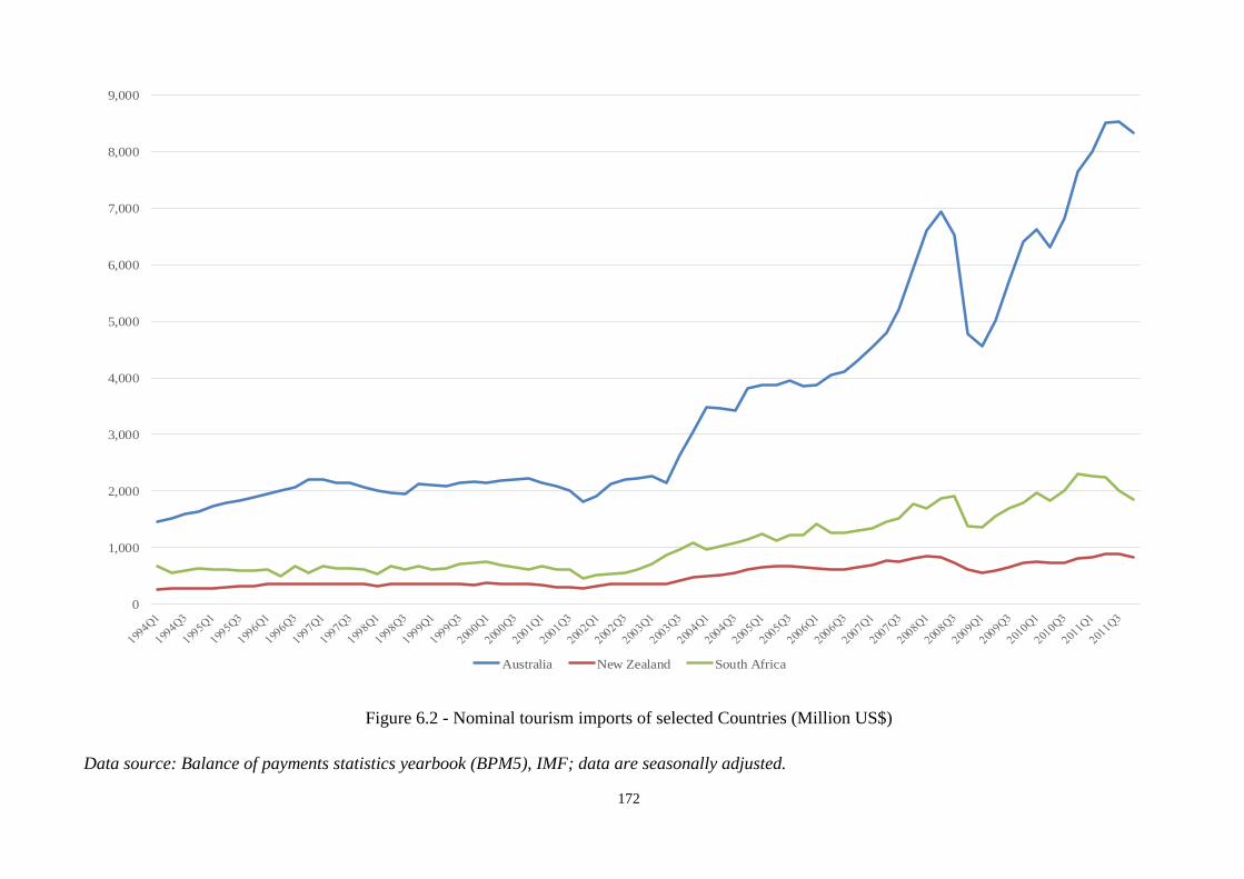
172
Figure 6.2 - Nominal tourism imports of selected Countries (Million US$)
Data source: Balance of payments statistics yearbook (BPM5), IMF; data are seasonally adjusted.
0
1,000
2,000
3,000
4,000
5,000
6,000
7,000
8,000
9,000
Australia New Zealand South Africa

173
Figure 6.3 - Nominal tourism imports of selected countries (Million US$)
Data source: Balance of payments statistics yearbook (BPM5), IMF; data are seasonally adjusted.
0
5,000
10,000
15,000
20,000
25,000
China India Japan Korea Malaysia Thailand
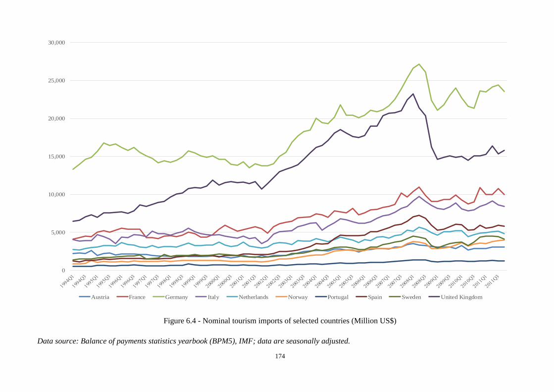
174
Figure 6.4 - Nominal tourism imports of selected countries (Million US$)
Data source: Balance of payments statistics yearbook (BPM5), IMF; data are seasonally adjusted.
0
5,000
10,000
15,000
20,000
25,000
30,000
Austria France Germany Italy Netherlands Norway Portugal Spain Sweden United Kingdom

175
Figure 6.5 - Nominal tourism exports of selected countries (Million US$)
Data source: Balance of payments statistics yearbook (BPM5), IMF; data are seasonally adjusted.
0
10,000
20,000
30,000
40,000
50,000
60,000
70,000
80,000
90,000
Argentina Brazil Canada Mexico USA
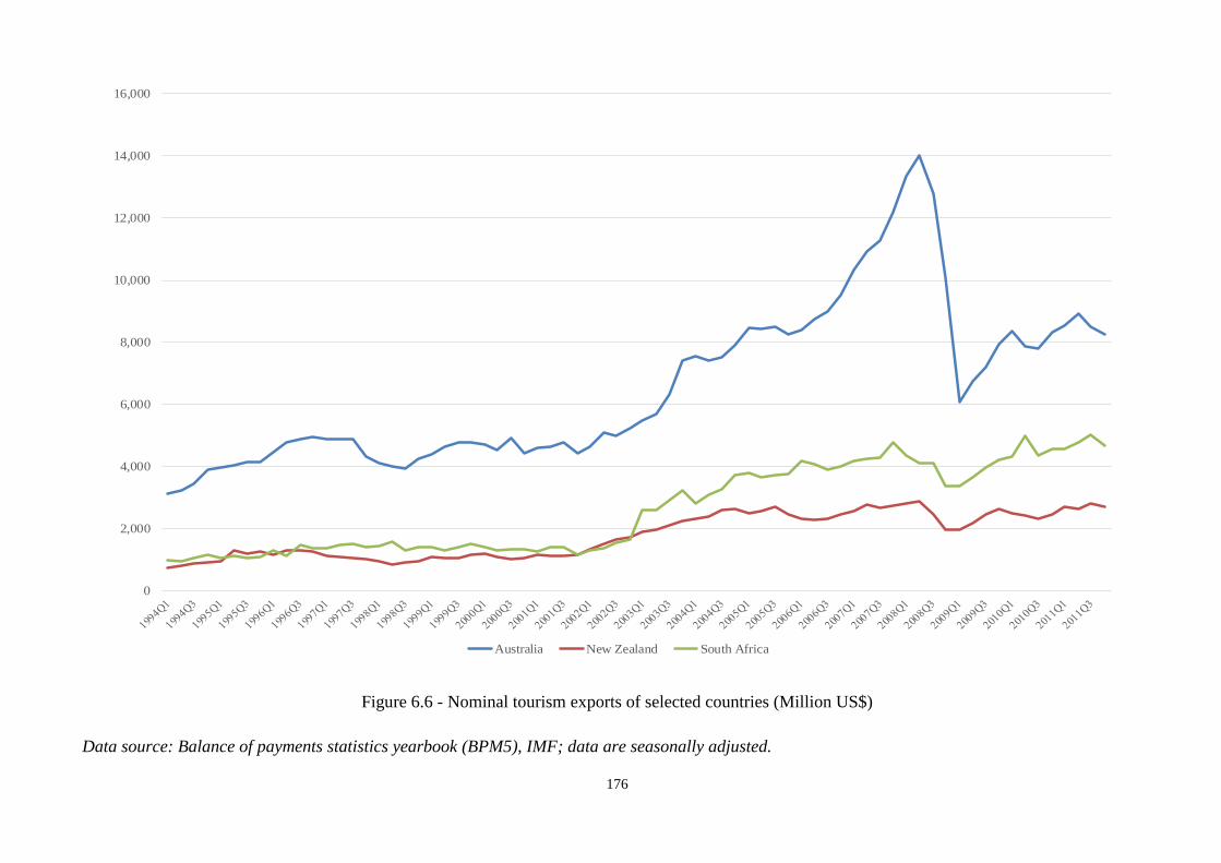
176
Figure 6.6 - Nominal tourism exports of selected countries (Million US$)
Data source: Balance of payments statistics yearbook (BPM5), IMF; data are seasonally adjusted.
0
2,000
4,000
6,000
8,000
10,000
12,000
14,000
16,000
Australia New Zealand South Africa
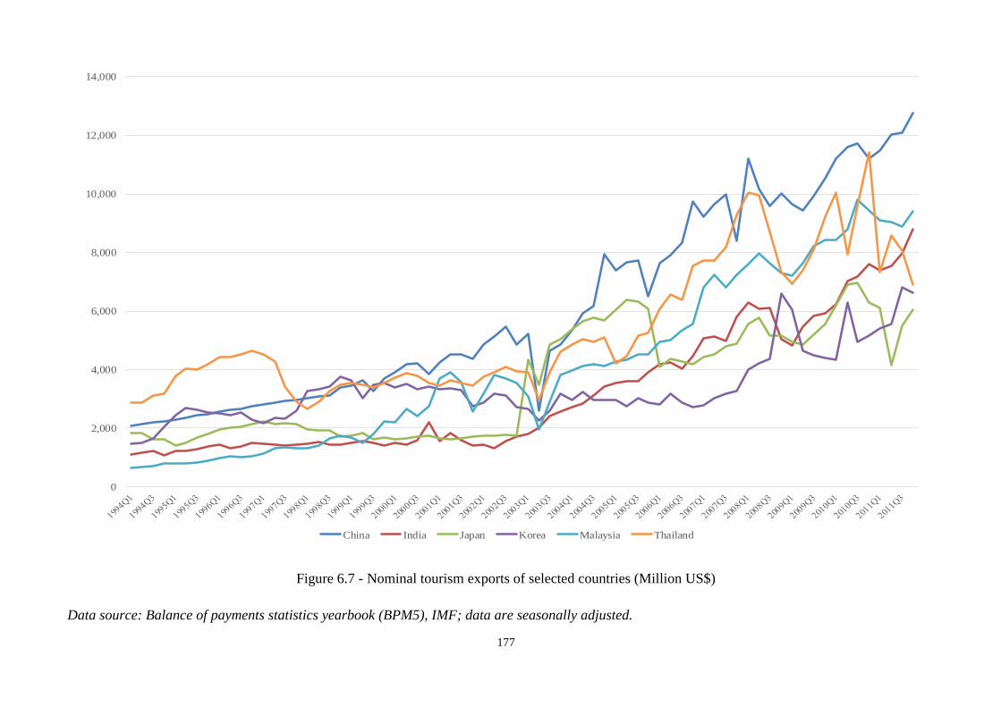
177
Figure 6.7 - Nominal tourism exports of selected countries (Million US$)
Data source: Balance of payments statistics yearbook (BPM5), IMF; data are seasonally adjusted.
0
2,000
4,000
6,000
8,000
10,000
12,000
14,000
China India Japan Korea Malaysia Thailand
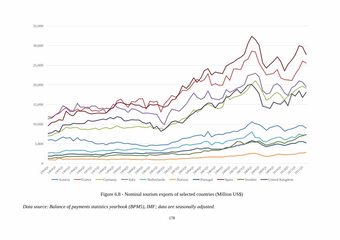
178
Figure 6.8 - Nominal tourism exports of selected countries (Million US$)
Data source: Balance of payments statistics yearbook (BPM5), IMF; data are seasonally adjusted.
0
5,000
10,000
15,000
20,000
25,000
30,000
35,000
Austria France Germany Italy Netherlands Norway Portugal Spain Sweden United Kingdom

179
Table 6.1 - Correlations of nominal tourism imports between major countries
Pearson Correlations
N=72 ARG AUS AUT BRA CAN CHN FRA DEU IND ITA JPN KOR
Argentina 1 .668** .368** .808** .654** .671** .463** .446** .593** .570** -.164 .353**
Australia .668** 1 .835** .940** .988** .953** .932** .910** .969** .936** -.106 .871**
Austria .368** .835** 1 .670** .858** .719** .892** .946** .812** .890** -.035 .859**
Brazil .808** .940** .670** 1 .916** .933** .784** .748** .883** .817** -.157 .711**
Canada .654** .988** .858** .916** 1 .935** .944** .922** .975** .944** -.147 .905**
China .671** .953** .719** .933** .935** 1 .869** .789** .957** .854** -.192 .771**
France .463** .932** .892** .784** .944** .869** 1 .958** .943** .949** -.120 .925**
Germany .446** .910** .946** .748** .922** .789** .958** 1 .884** .955** -.022 .914**
India .593** .969** .812** .883** .975** .957** .943** .884** 1 .916** -.181 .892**
Italy .570** .936** .890** .817** .944** .854** .949** .955** .916** 1 -.164 .877**
Japan -.164 -.106 -.035 -.157 -.147 -.192 -.120 -.022 -.181 -.164 1 -.099
Korea .353** .871** .859** .711** .905** .771** .925** .914** .892** .877** -.099 1
Malaysia .649** .973** .810** .907** .973** .965** .930** .875** .983** .926** -.240* .863**
Mexico .310** .806** .805** .605** .840** .762** .888** .837** .881** .840** -.213 .895**
Netherlands .530** .912** .889** .776** .921** .831** .956** .949** .897** .966** -.137 .868**
New
Zealand .521** .951** .884** .823** .961** .859** .943** .955** .937** .939** -.018 .944**
Norway .528** .963** .911** .833** .974** .890** .967** .965** .960** .965** -.108 .935**
Portugal .577** .935** .890** .807** .958** .843** .959** .964** .929** .975** -.144 .921**
South
Africa .618** .978** .865** .897** .980** .916** .936** .925** .952** .943** -.111 .884**
Spain .467** .911** .911** .744** .938** .823** .968** .964** .927** .960** -.153 .946**
Sweden .573** .964** .877** .847** .968** .878** .963** .959** .943** .960** -.095 .921**
Thailand .420** .847** .874** .750** .865** .757** .850** .868** .813** .803** .088 .874**
United
Kingdom .161 .688** .754** .437** .730** .574** .823** .828** .747** .790** -.100 .879**
USA .540** .870** .740** .723** .891** .832** .898** .847** .917** .891** -.156 .869**
Average .472 .821 .751 .717 .829 .758 .818 .808 .814 .813 -.116 .782
**. Correlation is significant at the 0.01 level (2-tailed).
*. Correlation is significant at the 0.05 level (2-tailed).
'Average' is the average of correlation coefficients excluding the particular country itself. Significance level is not shown
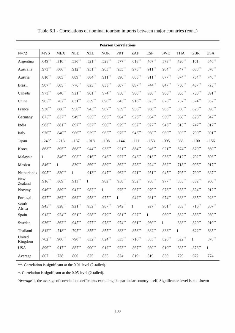
180
Table 6.1 - Correlations of nominal tourism imports between major countries (cont.)
Pearson Correlations
N=72 MYS MEX NLD NZL NOR PRT ZAF ESP SWE THA GBR USA
Argentina .649** .310** .530** .521** .528** .577** .618** .467** .573** .420** .161 .540**
Australia .973** .806** .912** .951** .963** .935** .978** .911** .964** .847** .688** .870**
Austria .810** .805** .889** .884** .911** .890** .865** .911** .877** .874** .754** .740**
Brazil .907** .605** .776** .823** .833** .807** .897** .744** .847** .750** .437** .723**
Canada .973** .840** .921** .961** .974** .958** .980** .938** .968** .865** .730** .891**
China .965** .762** .831** .859** .890** .843** .916** .823** .878** .757** .574** .832**
France .930** .888** .956** .943** .967** .959** .936** .968** .963** .850** .823** .898**
Germany .875** .837** .949** .955** .965** .964** .925** .964** .959** .868** .828** .847**
India .983** .881** .897** .937** .960** .929** .952** .927** .943** .813** .747** .917**
Italy .926** .840** .966** .939** .965** .975** .943** .960** .960** .803** .790** .891**
Japan -.240* -.213 -.137 -.018 -.108 -.144 -.111 -.153 -.095 .088 -.100 -.156
Korea .863** .895** .868** .944** .935** .921** .884** .946** .921** .874** .879** .869**
Malaysia 1 .846** .905** .916** .946** .927** .945** .915** .936** .812** .702** .896**
Mexico .846** 1 .830** .869** .889** .862** .828** .924** .862** .718** .906** .917**
Netherlands .905** .830** 1 .913** .947** .962** .921** .951** .945** .795** .790** .887**
New
Zealand .916** .869** .913** 1 .982** .958** .952** .958** .977** .855** .832** .900**
Norway .946** .889** .947** .982** 1 .975** .967** .979** .978** .855** .824** .912**
Portugal .927** .862** .962** .958** .975** 1 .942** .981** .974** .833** .835** .923**
South
Africa .945** .828** .921** .952** .967** .942** 1 .927** .961** .853** .716** .867**
Spain .915** .924** .951** .958** .979** .981** .927** 1 .960** .832** .885** .930**
Sweden .936** .862** .945** .977** .978** .974** .961** .960** 1 .833** .820** .910**
Thailand .812** .718** .795** .855** .855** .833** .853** .832** .833** 1 .622** .685**
United
Kingdom .702** .906** .790** .832** .824** .835** .716** .885** .820** .622** 1 .878**
USA .896** .917** .887** .900** .912** .923** .867** .930** .910** .685** .878** 1
Average .807 .738 .800 .825 .835 .824 .819 .819 .830 .729 .672 .774
**. Correlation is significant at the 0.01 level (2-tailed).
*. Correlation is significant at the 0.05 level (2-tailed).
'Average' is the average of correlation coefficients excluding the particular country itself. Significance level is not shown

181
Table 6.2 - Correlations of nominal tourism exports between major countries
Pearson Correlations
N=72 ARG AUS AUT BRA CAN CHN FRA DEU IND ITA JPN KOR
Argentina 1 .674** .760** .831** .788** .820** .718** .808** .884** .800** .587** .776**
Australia .674** 1 .847** .840** .882** .819** .932** .918** .793** .905** .787** .431**
Austria .760** .847** 1 .897** .820** .861** .883** .936** .897** .935** .812** .576**
Brazil .831** .840** .897** 1 .959** .979** .927** .970** .976** .883** .855** .756**
Canada .788** .882** .820** .959** 1 .958** .940** .953** .925** .871** .845** .683**
China .820** .819** .861** .979** .958** 1 .910** .952** .965** .849** .838** .758**
France .718** .932** .883** .927** .940** .910** 1 .967** .875** .921** .834** .616**
Germany .808** .918** .936** .970** .953** .952** .967** 1 .945** .950** .862** .665**
India .884** .793** .897** .976** .925** .965** .875** .945** 1 .876** .831** .771**
Italy .800** .905** .935** .883** .871** .849** .921** .950** .876** 1 .797** .577**
Japan .587** .787** .812** .855** .845** .838** .834** .862** .831** .797** 1 .536**
Korea .776** .431** .576** .756** .683** .758** .616** .665** .771** .577** .536** 1
Malaysia .824** .788** .842** .973** .944** .981** .889** .931** .962** .829** .811** .783**
Mexico .673** .924** .819** .917** .950** .915** .953** .943** .851** .860** .864** .558**
Netherlands .796** .891** .917** .967** .962** .950** .962** .980** .945** .927** .854** .659**
New
Zealand .586** .888** .847** .886** .910** .870** .926** .920** .840** .862** .919** .479**
Norway .862** .857** .941** .955** .915** .939** .905** .962** .971** .926** .817** .694**
Portugal .827** .898** .920** .975** .960** .959** .962** .987** .956** .933** .843** .703**
South
Africa .747** .875** .888** .952** .949** .934** .927** .959** .931** .897** .923** .606**
Spain .768** .932** .902** .958** .967** .936** .981** .987** .916** .932** .863** .630**
Sweden .888** .811** .889** .972** .927** .969** .897** .952** .980** .878** .773** .767**
Thailand .842** .830** .903** .894** .864** .897** .844** .912** .911** .890** .748** .627**
United
Kingdom .796** .924** .858** .890** .923** .878** .926** .945** .876** .940** .790** .551**
USA .903** .807** .813** .951** .942** .948** .884** .923** .949** .854** .754** .820**
Average .748 .802 .823 .882 .868 .870 .858 .889 .868 .837 .773 .626
**. Correlation is significant at the 0.01 level (2-tailed).
'Average' is the average of correlation coefficients excluding the particular country itself. Significance level is not shown.

182
Table 6.2 - Correlations of nominal tourism exports between major countries (cont.)
Pearson Correlations
N=72 MYS MEX NLD NZL NOR PRT ZAF ESP SWE THA GBR USA
Argentina .824** .673** .796** .586** .862** .827** .747** .768** .888** .842** .796** .903**
Australia .788** .924** .891** .888** .857** .898** .875** .932** .811** .830** .924** .807**
Austria .842** .819** .917** .847** .941** .920** .888** .902** .889** .903** .858** .813**
Brazil .973** .917** .967** .886** .955** .975** .952** .958** .972** .894** .890** .951**
Canada .944** .950** .962** .910** .915** .960** .949** .967** .927** .864** .923** .942**
China .981** .915** .950** .870** .939** .959** .934** .936** .969** .897** .878** .948**
France .889** .953** .962** .926** .905** .962** .927** .981** .897** .844** .926** .884**
Germany .931** .943** .980** .920** .962** .987** .959** .987** .952** .912** .945** .923**
India .962** .851** .945** .840** .971** .956** .931** .916** .980** .911** .876** .949**
Italy .829** .860** .927** .862** .926** .933** .897** .932** .878** .890** .940** .854**
Japan .811** .864** .854** .919** .817** .843** .923** .863** .773** .748** .790** .754**
Korea .783** .558** .659** .479** .694** .703** .606** .630** .767** .627** .551** .820**
Malaysia 1 .886** .935** .839** .923** .951** .906** .917** .962** .904** .836** .950**
Mexico .886** 1 .928** .926** .864** .927** .935** .960** .865** .818** .909** .865**
Netherlands .935** .928** 1 .928** .956** .987** .961** .983** .951** .903** .934** .915**
New
Zealand .839** .926** .928** 1 .860** .907** .951** .941** .832** .791** .875** .786**
Norway .923** .864** .956** .860** 1 .966** .925** .936** .966** .922** .903** .921**
Portugal .951** .927** .987** .907** .966** 1 .948** .984** .965** .918** .927** .936**
South
Africa .906** .935** .961** .951** .925** .948** 1 .961** .911** .857** .923** .873**
Spain .917** .960** .983** .941** .936** .984** .961** 1 .928** .880** .943** .907**
Sweden .962** .865** .951** .832** .966** .965** .911** .928** 1 .909** .887** .951**
Thailand .904** .818** .903** .791** .922** .918** .857** .880** .909** 1 .858** .880**
United
Kingdom .836** .909** .934** .875** .903** .927** .923** .943** .887** .858** 1 .874**
USA .950** .865** .915** .786** .921** .936** .873** .907** .951** .880** .874** 1
Average .857 .838 .883 .815 .870 .889 .864 .880 .868 .825 .840 .850
**. Correlation is significant at the 0.01 level (2-tailed).
'Average' is the average of correlation coefficients excluding the particular country itself. Significance level is not shown.
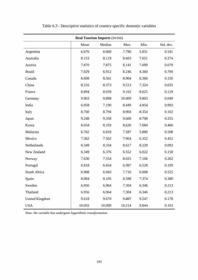
183
Table 6.3 - Descriptive statistics of country-specific domestic variables
Real Tourism Imports (lnrtim)
Mean Median Max. Min. Std. dev.
Argentina 6.676 6.660 7.786 5.831 0.541
Australia 8.153 8.119 8.603 7.651 0.274
Austria 7.870 7.875 8.141 7.699 0.079
Brazil 7.029 6.912 8.246 4.360 0.700
Canada 8.608 8.561 8.904 8.360 0.150
China 8.316 8.373 9.513 7.324 0.635
France 8.894 8.939 9.102 8.625 0.129
Germany 9.903 9.898 10.009 9.803 0.049
India 6.958 7.190 8.449 4.854 0.993
Italy 8.760 8.794 8.904 8.354 0.102
Japan 9.248 9.358 9.600 8.708 0.255
Korea 8.034 8.193 8.630 7.084 0.466
Malaysia 6.762 6.818 7.587 5.880 0.508
Mexico 7.362 7.502 7.904 6.352 0.452
Netherlands 8.349 8.334 8.617 8.228 0.093
New Zealand 6.349 6.376 6.552 6.022 0.158
Norway 7.630 7.554 8.025 7.166 0.262
Portugal 6.818 6.834 6.987 6.528 0.109
South Africa 6.908 6.943 7.716 6.008 0.525
Spain 8.084 8.105 8.588 7.374 0.380
Sweden 6.956 6.964 7.304 6.346 0.213
Thailand 6.956 6.964 7.304 6.346 0.213
United Kingdom 9.618 9.670 9.887 9.247 0.178
USA 10.055 10.090 10.214 9.844 0.103
Note: the variable has undergone logarithmic transformation
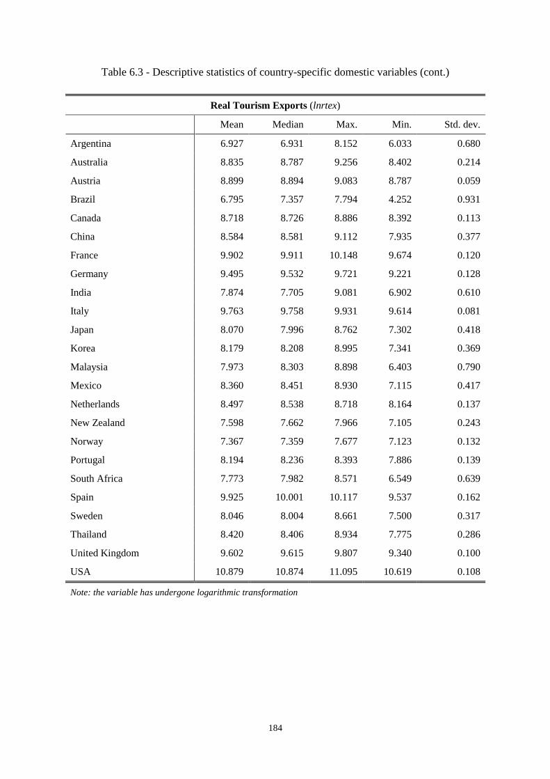
184
Table 6.3 - Descriptive statistics of country-specific domestic variables (cont.)
Real Tourism Exports (lnrtex)
Mean Median Max. Min. Std. dev.
Argentina 6.927 6.931 8.152 6.033 0.680
Australia 8.835 8.787 9.256 8.402 0.214
Austria 8.899 8.894 9.083 8.787 0.059
Brazil 6.795 7.357 7.794 4.252 0.931
Canada 8.718 8.726 8.886 8.392 0.113
China 8.584 8.581 9.112 7.935 0.377
France 9.902 9.911 10.148 9.674 0.120
Germany 9.495 9.532 9.721 9.221 0.128
India 7.874 7.705 9.081 6.902 0.610
Italy 9.763 9.758 9.931 9.614 0.081
Japan 8.070 7.996 8.762 7.302 0.418
Korea 8.179 8.208 8.995 7.341 0.369
Malaysia 7.973 8.303 8.898 6.403 0.790
Mexico 8.360 8.451 8.930 7.115 0.417
Netherlands 8.497 8.538 8.718 8.164 0.137
New Zealand 7.598 7.662 7.966 7.105 0.243
Norway 7.367 7.359 7.677 7.123 0.132
Portugal 8.194 8.236 8.393 7.886 0.139
South Africa 7.773 7.982 8.571 6.549 0.639
Spain 9.925 10.001 10.117 9.537 0.162
Sweden 8.046 8.004 8.661 7.500 0.317
Thailand 8.420 8.406 8.934 7.775 0.286
United Kingdom 9.602 9.615 9.807 9.340 0.100
USA 10.879 10.874 11.095 10.619 0.108
Note: the variable has undergone logarithmic transformation

185
Table 6.3 - Descriptive statistics of country-specific domestic variables (cont.)
Real Income (lny)
Mean Median Max. Min. Std. dev.
Argentina 0.060 0.065 0.280 -0.186 0.114
Australia -0.034 -0.018 0.030 -0.134 0.050
Austria 0.006 0.013 0.051 -0.060 0.028
Brazil -0.401 -0.413 -0.294 -0.463 0.044
Canada -0.035 -0.026 0.007 -0.098 0.034
China -0.145 -0.184 0.505 -0.676 0.364
France 0.000 0.015 0.051 -0.099 0.045
Germany 0.045 0.056 0.130 -0.070 0.062
India -0.069 -0.126 0.343 -0.350 0.218
Italy 0.013 0.044 0.108 -0.160 0.079
Japan 0.027 0.032 0.163 -0.146 0.090
Korea -0.062 -0.029 0.088 -0.283 0.106
Malaysia -0.061 -0.077 0.137 -0.320 0.116
Mexico -0.019 -0.011 0.050 -0.168 0.044
Netherlands 0.005 0.004 0.063 -0.071 0.034
New Zealand -0.057 -0.063 0.007 -0.114 0.033
Norway -0.018 -0.008 0.040 -0.098 0.035
Portugal -0.003 -0.007 0.094 -0.151 0.061
South Africa -0.022 -0.038 0.059 -0.088 0.050
Spain -0.051 -0.036 0.022 -0.137 0.049
Sweden -0.030 -0.021 0.029 -0.092 0.030
Thailand -0.032 -0.015 0.084 -0.179 0.070
United Kingdom -0.039 -0.032 0.018 -0.110 0.036
USA -0.036 -0.018 0.013 -0.095 0.036
Note: the variable has undergone logarithmic transformation

186
Table 6.3 - Descriptive statistics of country-specific domestic variables (cont.)
Own Price (lnp)
Mean Median Max. Min. Std. dev.
Argentina 0.275 0.178 0.611 -0.396 0.306
Australia -0.116 -0.189 0.509 -0.506 0.287
Austria -0.088 -0.119 0.298 -0.449 0.213
Brazil 0.095 0.176 0.711 -0.628 0.325
Canada -0.116 -0.274 0.339 -0.397 0.243
China 0.021 -0.057 0.466 -0.447 0.198
France -0.085 -0.103 0.291 -0.447 0.205
Germany -0.074 -0.088 0.292 -0.429 0.199
India -0.047 -0.177 0.482 -0.364 0.235
Italy -0.106 -0.169 0.299 -0.468 0.228
Japan 0.031 0.017 0.345 -0.211 0.127
Korea -0.128 -0.127 0.164 -0.647 0.183
Malaysia 0.060 0.072 0.264 -0.197 0.134
Mexico -0.112 -0.058 0.184 -0.696 0.200
Netherlands -0.107 -0.164 0.282 -0.470 0.218
New Zealand -0.184 -0.184 0.352 -0.647 0.266
Norway -0.103 -0.159 0.299 -0.439 0.217
Portugal -0.125 -0.212 0.315 -0.498 0.245
South Africa -0.112 -0.074 0.309 -0.745 0.219
Spain -0.122 -0.221 0.336 -0.502 0.256
Sweden -0.048 -0.046 0.292 -0.392 0.173
Thailand 0.080 0.074 0.479 -0.309 0.201
United Kingdom -0.123 -0.167 0.173 -0.389 0.154
USA -0.064 -0.070 0.148 -0.286 0.131
Note: the variable has undergone logarithmic transformation

187
Table 6.4 - Descriptive statistics of country-specific foreign variables
Real Tourism Imports (lnrtim*)
Mean Median Max. Min. Std. dev.
Argentina 8.323 8.286 8.793 7.678 0.222
Australia 8.737 8.759 8.852 8.571 0.067
Austria 9.381 9.409 9.476 9.232 0.073
Brazil 8.787 8.838 9.001 8.561 0.133
Canada 9.739 9.764 9.870 9.531 0.093
China 9.018 9.037 9.103 8.851 0.059
France 9.004 9.046 9.139 8.818 0.097
Germany 8.665 8.729 8.800 8.413 0.127
India 8.989 8.987 9.063 8.842 0.039
Italy 8.992 9.039 9.096 8.830 0.091
Japan 8.847 8.909 9.094 8.558 0.156
Korea 9.007 9.011 9.131 8.801 0.059
Malaysia 9.010 9.026 9.122 8.841 0.065
Mexico 9.764 9.773 9.938 9.559 0.089
Netherlands 9.170 9.200 9.270 9.056 0.066
New Zealand 8.795 8.822 8.946 8.587 0.104
Norway 8.885 8.914 9.090 8.659 0.136
Portugal 8.808 8.846 8.946 8.576 0.109
South Africa 8.941 9.060 9.141 8.399 0.240
Spain 8.857 8.883 8.963 8.718 0.072
Sweden 8.972 9.006 9.083 8.802 0.085
Thailand 8.965 8.984 9.095 8.778 0.072
United Kingdom 8.893 8.939 9.000 8.686 0.096
USA 8.467 8.460 8.756 8.200 0.152
Note: the variable has undergone logarithmic transformation

188
Table 6.4 - Descriptive statistics of country-specific foreign variables (cont.)
Real Tourism Exports (lnrtex*)
Mean Median Max. Min. Std. dev.
Argentina 8.622 8.781 8.955 7.999 0.276
Australia 8.915 8.908 9.136 8.534 0.170
Austria 9.451 9.502 9.637 9.147 0.133
Brazil 9.186 9.239 9.426 8.907 0.175
Canada 10.401 10.428 10.531 10.169 0.092
China 9.073 9.025 9.375 8.649 0.199
France 9.395 9.431 9.553 9.147 0.110
Germany 9.275 9.314 9.434 9.007 0.121
India 9.328 9.348 9.483 9.085 0.104
Italy 9.389 9.443 9.558 9.128 0.127
Japan 9.402 9.423 9.558 9.160 0.100
Korea 9.140 9.117 9.388 8.812 0.145
Malaysia 9.142 9.100 9.372 8.776 0.167
Mexico 10.436 10.440 10.626 10.266 0.087
Netherlands 9.422 9.450 9.566 9.216 0.096
New Zealand 9.086 9.097 9.355 8.729 0.171
Norway 9.225 9.236 9.441 8.921 0.148
Portugal 9.536 9.588 9.737 9.197 0.152
South Africa 9.186 9.270 9.397 8.676 0.223
Spain 9.334 9.362 9.456 9.131 0.088
Sweden 9.167 9.186 9.320 8.960 0.094
Thailand 8.983 8.982 9.231 8.539 0.183
United Kingdom 9.333 9.364 9.485 9.034 0.129
USA 8.619 8.640 8.884 8.116 0.230
Note: the variable has undergone logarithmic transformation

189
Table 6.4 - Descriptive statistics of country-specific foreign variables (cont.)
Real Income (lny*)
Mean Median Max. Min. Std. dev.
Argentina -0.133 -0.146 -0.056 -0.168 0.030
Australia -0.006 -0.024 0.101 -0.055 0.043
Austria 0.019 0.033 0.063 -0.064 0.040
Brazil 0.010 0.006 0.095 -0.030 0.030
Canada -0.027 -0.017 0.006 -0.077 0.026
China -0.008 -0.002 0.015 -0.061 0.020
France -0.005 0.000 0.024 -0.056 0.021
Germany -0.014 -0.009 0.014 -0.042 0.016
India -0.003 -0.010 0.067 -0.034 0.028
Italy -0.003 -0.001 0.022 -0.043 0.015
Japan -0.027 -0.047 0.135 -0.139 0.080
Korea -0.003 -0.033 0.128 -0.055 0.054
Malaysia 0.000 -0.009 0.069 -0.030 0.027
Mexico -0.027 -0.017 0.009 -0.074 0.025
Netherlands 0.005 0.011 0.032 -0.043 0.019
New Zealand -0.012 -0.017 0.060 -0.064 0.034
Norway -0.011 -0.006 0.018 -0.061 0.021
Portugal -0.013 -0.007 0.019 -0.076 0.026
South Africa -0.022 -0.008 0.053 -0.124 0.048
Spain 0.000 0.007 0.036 -0.059 0.026
Sweden -0.005 0.000 0.025 -0.050 0.019
Thailand 0.001 -0.004 0.064 -0.025 0.023
United Kingdom -0.001 -0.001 0.026 -0.037 0.014
USA -0.016 -0.019 0.062 -0.065 0.034
Note: the variable has undergone logarithmic transformation
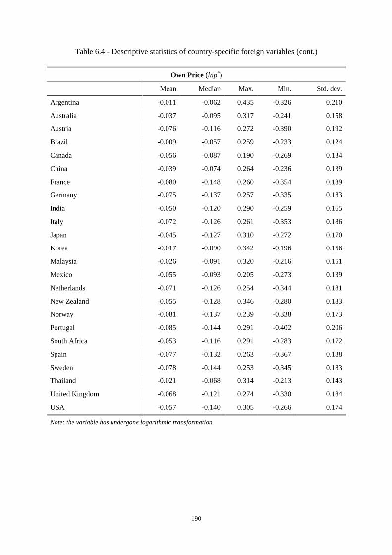
190
Table 6.4 - Descriptive statistics of country-specific foreign variables (cont.)
Own Price (lnp*)
Mean Median Max. Min. Std. dev.
Argentina -0.011 -0.062 0.435 -0.326 0.210
Australia -0.037 -0.095 0.317 -0.241 0.158
Austria -0.076 -0.116 0.272 -0.390 0.192
Brazil -0.009 -0.057 0.259 -0.233 0.124
Canada -0.056 -0.087 0.190 -0.269 0.134
China -0.039 -0.074 0.264 -0.236 0.139
France -0.080 -0.148 0.260 -0.354 0.189
Germany -0.075 -0.137 0.257 -0.335 0.183
India -0.050 -0.120 0.290 -0.259 0.165
Italy -0.072 -0.126 0.261 -0.353 0.186
Japan -0.045 -0.127 0.310 -0.272 0.170
Korea -0.017 -0.090 0.342 -0.196 0.156
Malaysia -0.026 -0.091 0.320 -0.216 0.151
Mexico -0.055 -0.093 0.205 -0.273 0.139
Netherlands -0.071 -0.126 0.254 -0.344 0.181
New Zealand -0.055 -0.128 0.346 -0.280 0.183
Norway -0.081 -0.137 0.239 -0.338 0.173
Portugal -0.085 -0.144 0.291 -0.402 0.206
South Africa -0.053 -0.116 0.291 -0.283 0.172
Spain -0.077 -0.132 0.263 -0.367 0.188
Sweden -0.078 -0.144 0.253 -0.345 0.183
Thailand -0.021 -0.068 0.314 -0.213 0.143
United Kingdom -0.068 -0.121 0.274 -0.330 0.184
USA -0.057 -0.140 0.305 -0.266 0.174
Note: the variable has undergone logarithmic transformation

191
Table 6.5 - Descriptive statistics of global common variable
Oil Price (lnpoil)
Mean Median Max. Min. Std. dev.
-0.435 -0.614 0.820 -1.522 0.673
Note: the variable has undergone a logarithmic transformation
To summarise the pair-wise correlations, a simple statistic is the arithmetic average.
The bottom rows of both Table 6.1 and Table 6.2 calculate the averages of
correlations for each country (excluding the particular country itself, i.e., the entries
that are 1). In terms of tourism imports, the average pair-wise correlation of many
countries stands at between .472 and .835, except for Japan which is -.116. Almost all
the pair-wise correlations of Japan are statistically insignificant. This is in line with
Figure 6.3, which shows stagnant changes of Japan’s tourism imports over the years.
In terms of tourism exports, the magnitude of the correlations is generally higher,
ranging between .626 and .889.
While the pair-wise correlation indicates how interconnected tourism trade (or
international tourism demand) is, it does not offer much explanatory power with
regard to the underlying causal relationship. A detailed assessment of
interdependencies of international tourism demand has to rely on econometric models.
Variables in Real Terms
As proposed in Chapter 5, real macroeconomic variables and real tourism trade
variables will be used in the GVAR modelling approach. Table 6.3 – Table 6.5 show
the basic descriptive statistics of all the variables. The real term variables are the
actual variables used in the current research’s modelling exercise and they have all
undergone logarithm transformation. This is in line with other existing studies on
tourism trade.
To interpret these descriptive statistics, one can take exponential of the mean and
median statistics to obtain the original levels of respective variables. The mean and
median numbers are for the sample period, i.e., 1994Q1 to 2011Q4. A straightforward
way of making sense of these statistics is to simply compare the mean and median
across different countries. The higher the statistics, the larger volume a country has.

192
From Table 6.3, it is shown that the USA has the largest volume of real tourism
imports and real tourism exports, as its mean (10.055) is higher than any other
country’s. The other countries that have relatively large volumes of real tourism trade
are Germany, Japan, and the UK, according to their mean figures. The std.dev.
(standard deviation) column shows how volatile during the sample period the real
tourism trade figures are. On the one hand, among all the 24 countries, Austria has
seen a relatively stable real tourism trade, as its std.dev. maintains at 0.079 and 0.059.
On the other hand, emerging countries and developing countries such as Argentina,
Brazil, India, Malaysia, and South Africa are among the countries which have seen
substantial fluctuations of real tourism trade over the years.
With regard to the real income variable and the own price variable in Table 6.3, the
std.dev. column shows a clear pattern that over the sample period, emerging countries
such as Argentina, China and India have witnessed remarkable developments in terms
of real income. For other countries (mostly developed countries), their real income
levels remain relatively stable. Meanwhile, all the 24 countries have seen their own
price level varying greatly over the sample period. Hence, compared with the real
income variable, the own price variable may play a more important role in explaining
the fluctuations of real tourism trade.
Table 6.4 reports the descriptive statistics of each country’s foreign variables, which
are the weighted averages of each country’s foreign counterparts. The foreign
variables are supposed to be proxies for a country’s external economic performance.
The mean values of these foreign variables are relatively similar for different
countries.

193
Table 6.6 - Order of integration of each variable
Real
Tourism
Imports
Real
Tourism
Exports
Real Income Own price
Foreign
Tourism
Imports
Foreign
Tourism
Exports
Foreign
Real Income
Foreign
Prices
(lnrtim) (lnrtex) (lny) (lnp) (lnrtim*) (lnrtex*) (lny*) (lnp*)
Argentina 1 1 1 1 1 1 1 1
Australia 0 1 1 1 1 1 1 1
Austria 1 0 1 1 1 1 1 1
Brazil 1 1 1 1 0 1 1 1
Canada 1 1 1 1 1 1 1 1
China 0 0 1 1 0 1 0 1
France 1 1 1 1 1 1 1 1
Germany 1 1 1 1 1 1 1 1
India 1 1 1 1 1 1 1 1
Italy 0 1 1 1 1 1 1 1
Japan 1 1 1 1 1 1 1 1
Korea 1 1 0 1 1 1 1 1
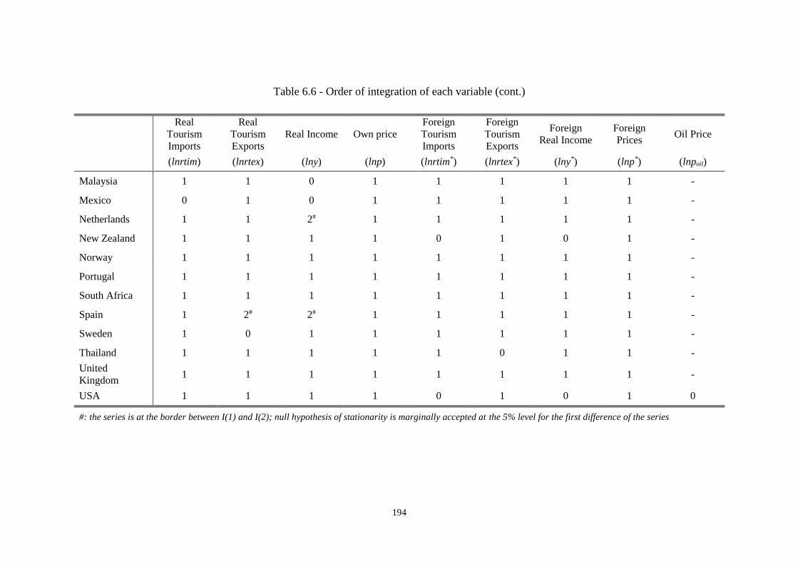
194
Table 6.6 - Order of integration of each variable (cont.)
Real
Tourism
Imports
Real
Tourism
Exports
Real Income Own price
Foreign
Tourism
Imports
Foreign
Tourism
Exports
Foreign
Real Income
Foreign
Prices Oil Price
(lnrtim) (lnrtex) (lny) (lnp) (lnrtim*) (lnrtex*) (lny*) (lnp*) (lnpoil)
Malaysia 1 1 0 1 1 1 1 1 -
Mexico 0 1 0 1 1 1 1 1 -
Netherlands 1 1 2# 1 1 1 1 1 -
New Zealand 1 1 1 1 0 1 0 1 -
Norway 1 1 1 1 1 1 1 1 -
Portugal 1 1 1 1 1 1 1 1 -
South Africa 1 1 1 1 1 1 1 1 -
Spain 1 2# 2# 1 1 1 1 1 -
Sweden 1 0 1 1 1 1 1 1 -
Thailand 1 1 1 1 1 0 1 1 -
United
Kingdom 1 1 1 1 1 1 1 1 -
USA 1 1 1 1 0 1 0 1 0
#: the series is at the border between I(1) and I(2); null hypothesis of stationarity is marginally accepted at the 5% level for the first difference of the series

195
6.2.2 Unit Root Tests
Table 6.6 reports the results of unit root tests. A unit root test aims to find out whether
a variable, for instance real tourism imports, evolves over time in a random manner or
a stationary manner. The unit root test results will decide the appropriateness of the
model specification proposed in Section 5.2.2. As described in Section 5.2.2, the
augmented Dickey-Fuller (ADF) test and the weighted symmetric versions of ADF
(WS-ADF) test are used. As long as one of ADF and WS-ADF indicates stationarity
of a variable, whether at its level, first difference or second difference, the variable (or
its differenced term) will be deemed stationary. The test results are according to
critical values at the 5% significance level.
It is obvious that across all the countries sampled in the current research, the variables
are I(1) series in most cases, with occasional I(0) series. The real tourism exports
(lnrtex) of Spain and the real income (lny) for both Netherlands and Spain are found
to be I(2), at the 5% significance level. They are marginal cases. For both domestic
own price (lnp) and foreign prices (lnp*), they are I(1) series across all the countries.
The oil price variable, which is global common variable, is marginally accepted as
I(0) series.
Given that the GVAR approach is able to work with both I(0) and I(1) series, the unit
root test results above confirm that the data set meet the requirements.
6.3 Model Estimation Results
The global VAR (GVAR) modelling approach is able to generate a large set of
estimation results, due to the potential number of endogenous variables included in
the model.
As discussed in Section 5.2.2, one of the focuses is the matrix 𝜦𝑖0 in Eq. (5.8), which
captures the contemporaneous effects of foreign variables on their domestic
counterparts, for example, the percentage change of a particular country’s tourism
exports (rtex) in response to 1 percent change of other countries’ tourism exports
(rtex*). Another focus is the impulse responses to shocks. The impacts of shocks to
China’s macroeconomic variables on all other countries’ tourism trade will be
simulated. All of these provide a quantitative picture of the degree of
interdependencies between major countries around the world.

196
Table 6.7 - Lag orders of country-specific VECMX models
Lag order of domestic
variables (pi)
Lag order of foreign
variables (qi)
Argentina 2 2
Australia 2 1
Austria 2 2
Brazil 1 2
Canada 2 1
China 3 2
France 1 1
Germany 2 2
India 1 1
Italy 2 1
Japan 2 1
Korea 2 1
Malaysia 2 3
Mexico 2 1
Netherlands 1 1
New Zealand 1 1
Norway 1 1
Portugal 3 2
South Africa 1 1
Spain 2 2
Sweden 1 1
Thailand 3 2
United Kingdom 3 3
USA 2 1
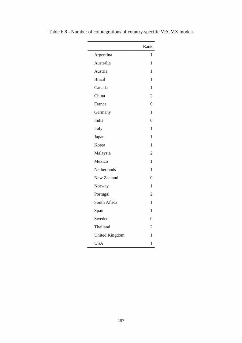
197
Table 6.8 - Number of cointegrations of country-specific VECMX models
Rank
Argentina 1
Australia 1
Austria 1
Brazil 1
Canada 1
China 2
France 0
Germany 1
India 0
Italy 1
Japan 1
Korea 1
Malaysia 2
Mexico 1
Netherlands 1
New Zealand 0
Norway 1
Portugal 2
South Africa 1
Spain 1
Sweden 0
Thailand 2
United Kingdom 1
USA 1

198
6.3.1 Model Specification Parameters
The most important parameters concerning the first stage country-specific VECMX
models are the lag orders of domestic variables and foreign variables, which are
described in Section 5.2.2, i.e., pi and qi in Eq. (5.8), and the number of cointegrating
relations among endogenous domestic variables, weakly exogenous foreign variables
and weakly exogenous global common variable, i.e., ri in Eq. (5.8). Table 6.7 and
Table 6.8 shows the final choices of these parameters.
As described in Section 5.3.3, the determination of lag orders is through comparing
the preliminary GVAR estimation results under different maximum lag order settings.
In the same vein, the final choice of the rank order of each VECMX model depends
on whether a lower rank will generate better estimation results. This is done by
manually setting the rank order to 2 or 1, if the rank is initially found to be above 2
according to trace statistics. Pesaran, Schuermann, and Smith (2009) describe a
similar strategy to achieve better model specifications. All in all, it is found that lower
lag orders as well as lower rank orders tend to produce better results, in terms of
acceptable diagnostic test results and reasonable persistence profiles.
In the cases where the rank order is zero, the country-specific VECMX model as Eq.
(5.8) will be replaced by differenced VAR model augmented with exogenous
variables (VARX). That is equivalent to Eq. (5.8) without the 𝜶𝑖𝜷𝑖′[𝒛𝑖,𝑡−1 −
𝜸𝑖(𝑡 − 1)] part.
In total, there are 24 cointegrating relations identified among the countries sampled in
the current research. Each of them denotes an equilibrium state where the domestic
variables, foreign variables and global common variables have a stable and consistent
relationship.
6.3.2 Contemporaneous Impact Elasticities
One set of the main results from the GVAR approach are the contemporaneous impact
elasticities between domestic variables and their corresponding foreign variables in
the first stage VECMX models. They show how much a country’s economy will
change (or be affected) if its external environment changes. They are particularly
useful in the GVAR approach in order to identify general co-movements among
variables across different countries (Galesi & Lombardi, 2009). The concept of

199
elasticity, which measures the change of a target variable in response to a one-percent
change of its explanatory variable, is widely applied in tourism demand analysis. It is
a simple indicator of the relationship between a target variable and its explanatory
variable. For tourism practitioners, it would be of their interests to know about the
changes of their native market’s tourism demand (inbound and outbound) in response
to changes of explanatory factors, especially if they are operating at different
destination countries. So they can react differently in different destinations. Tourism
demand for a destination country directly affects the performance of tourism
businesses, in terms of their revenues and profits.
Specifically, the contemporaneous impact elasticities, which come from 𝚲𝑖0 in Eq.
(5.8), are reported in Table 6.9. They are the coefficients on the weakly exogenous
foreign variables 𝒙𝑖𝑡∗ , when the endogenous domestic variables 𝒙𝑖𝑡 are the ‘dependent’
variables1. Similar to demand elasticities, a contemporaneous impact elasticities
denotes the percentage change of 𝒙𝑖𝑡 in response to 1% change in 𝒙𝑖𝑡∗ , at time t. For
example, an impact elasticity of 0.5 for real tourism exports (lnrtex) in the first stage
VECMX model implies that, if on average the other countries’ tourism exports (i.e.,
foreign tourism exports, lnrtex*) increases by 1%, then the tourism exports (lnrtex) of
the country concerned would accordingly increase by 0.5%.
‘Contemporaneous’ means 𝒙𝑖𝑡 and 𝒙𝑖𝑡∗ are at time t, and no lagged effects from time t-
1, t-2, …, are involved. For one thing, this is in line with the practice of reporting in
existing economic studies using the GVAR approach, for example, Vansteenkiste and
Hiebert (2011), Dees, Mauro, Pesaran, and Smith (2007), Galesi and Lombardi
(2009). Contemporaneous effects are also a good indicator of synchronisation of
business cycles, since contemporaneity means the effects are immediate. For another,
it is difficult to track the dynamic effects (lagged effects) between variables within a
VAR model setting, given that there are too many variables involved simultaneously.
General Observations
1 Strictly speaking, there are no ‘dependent’ and ‘independent’ variables in a vector autoregressive
(VAR) model, since all variables are supposed to be ‘dependent’ and ‘independent’ variables in the
same model. So instead, the distinction could be made between ‘endogenous’ and ‘exogenous’
variables in a conditional VAR model, see Garratt, Lee, Pesaran, and Shin (2012, pp.57-59).

200
Statistically significant impact elasticities are widely observed in Table 6.9. All the 24
countries in the current research have at least one statistically significant impact
elasticity. This confirms the existence of dependencies on external world for the
major countries around the world. While this finding is not entirely new nor
surprising, the results in the table measure how intense such dependencies are. The
value of the impact elasticities ranges between 0.348 and 1.958 for real tourism
imports, 0.373 and 0.841 for real tourism exports, 0.408 and 2.360 for real income,
0.109 and 1.715 for own price (excluding all insignificant numbers).
There is, however, no definitive pattern among the 24 countries. Countries with three
significant impact elasticities are notably Brazil, France, India, Italy, the Netherlands,
Norway and Spain. They are predominantly European countries, and can be seen as
more interconnected with other countries’ international tourism sector. In other words,
the international tourism trade of these countries is easily affected by the general
economic performance around the world. Monitoring the macroeconomic trends is of
particular importance to these countries, especially in times of global economic
turbulence.
Real Tourism Imports and Real Tourism Exports
Above half of the 24 countries in the current research see either their tourism imports
(i.e., outbound demand) or their tourism exports (i.e., inbound demand) depend on
their foreign counterparts. In many cases, the contemporaneous impact elasticities are
between 0.5 and 1 (see column Real Tourism Imports and Real Tourism Exports in
Table 6.9), meaning a country’s response to external world changes is rather moderate
and not very sensitive. For example, the contemporaneous impact elasticity for
Australia’s real tourism imports is 0.590. It means that, if the value of outbound
tourism of other countries increases by 1%, then the value of Australia’s outbound
tourism will correspondingly increase by 0.590%. Hence, Australia’s outbound
tourism follows the general trend of other countries to a moderate extent. On the
contrary, the impact elasticities for real income and own price are almost unanimously
significant and sensitive across all the 24 countries.
The less sensitive elasticities of tourism trade variables may well be linked to the fact
that tourism interdependency is not only an economic phenomenon, but is also
influenced by non-economic factors. Admittedly, the contemporaneous impact
201
elasticities obtained from the GVAR approach only consider the impacts of economic
changes, since the variables in the current research are measured in economic terms.
However, at the macro level and international level, tourism embodies the process of
globalisation, which as discussed in Section 4.3 is driven by not only economic
forces, but also technological, political and cultural forces. Even though the foreign
variables (those with a star *) are understood to be proxies for unobserved global
common factors (including global common non-economic factors), the country-
specific non-economic factors are still omitted by the model. Hence, persistence
resulting from non-economic factors may exist for a country’s tourism demand, and it
reduces the sensitivity of the country’s dependency on external economic changes
alone. For example, tourist flows in and out of a country can be manipulated through
border controls and visa regulations (a country-specific non-economic factor), which
in turn certainly alternate the contemporaneous impact elasticities had there been only
economic forces in place.
It can be seen as a shortcoming of the GVAR approach, which indeed is also a general
shortcoming of econometric models, in the sense that only measurable factors are
considered in a model (and it happens that measurable factors tend to be economic
ones, see Section 2.4.1 for extensive discussions). But within the topic of
interdependencies, it remains that compared to non-economic factors, economic
factors tend to be more volatile and are much more mutually influencing across
countries. Endogeneity, which the GVAR approach is set out to tackle, is more
‘rampant’ among economic factors, rather than among country-specific non-economic
factors.
Nevertheless, the results in Table 6.9 show that there is a certain level of
interdependency of tourism trade for many countries. Hence, the economic
performance of international tourism sector across many countries is found to be
somewhat synchronised.
Real Income and Own price
Contemporaneous impact elasticities for real income and own price are mostly
significant. Almost every one of the 24 countries sees its real income as well as its
own price (i.e., consumer price index adjusted by exchange rates against US dollar)
co-move with the other countries.

202
Table 6.9 - Contemporaneous effects of foreign variables on domestic variables
Real Tourism Imports Real Tourism Exports Real Income Own price
(lnrtim*, lnrtim) (lnrtex*, lnrtex) (lny*, lny) (lnp*, lnp)
Argentina - 0.136 0.624* -0.149
Australia 0.590*** 0.006 - -
Austria -0.641 -0.017 0.639*** 1.163***
Brazil 0.776* 0.882 0.847*** 1.088*
Canada 0.348*** - - -
China 0.010 0.368 0.599** 0.109*
France 0.406 0.752** 0.809*** 1.300***
Germany -0.071 0.187 0.920*** 1.436***
India 1.958* 0.153 0.739*** 0.774***
Italy 0.373 0.841*** 0.852*** 1.336***
Japan - - 0.776*** 0.614
Korea -0.009 -0.479 0.886*** 0.438
Malaysia - - 1.082*** 0.848***
Mexico 0.824** 0.261 2.360*** 0.203
Netherlands 0.553 0.506* 0.827*** 1.349***
New Zealand 0.394 -0.324 0.796*** 1.715***
Norway 0.732*** 0.008 0.903** 1.077***
Portugal 0.352 0.548** 0.964*** -
South Africa 0.154 0.864 0.408*** 1.262***
Spain 0.351 0.373* 0.982*** 1.298***
Sweden 0.857 0.121 1.358*** 1.280***
Thailand 1.212*** -0.070 0.551 1.461***
United Kingdom 0.146 0.042 0.637*** 0.553***
USA 0.551*** 0.077 - 0.140***
***, **, *: statistically significant at the 1%, 5% and 10% level, respectively
The numbers denote the percentage change of domestic variable in response to 1% change in foreign variable
Domestic variables are lnrtim, lnrtex, lny and lnp; foreign variables are lnrtim*, lnrtex*, lny* and
lnp*
-: The foreign variable is not used, since it is not weakly exogenous in the VECMX model; no impact elasticity is
derived

203
For real income, the elasticities are usually between 0.7 and 1, more sensitive than
those of tourism trade variables. These results are generally consistent with those
reported in other economic studies, such as Dees, Holly, Pesaran, and Smith (2007),
Dees, Mauro, Pesaran, and Smith (2007), and Galesi and Lombardi (2009). For own
price, the elasticities are even more sensitive, generally standing between 1 and 1.5.
But there are some countries which have insignificant elasticities of own price. They
tend to be Asian countries or emerging economies.
Overall, real income and own price are more prominent channels through which an
economy is influenced by its external environment. As opposed to tourism trade
variables, real income and own price are both principally economic-related. As long
as a country is actively engaging in cross-country economic activities, co-movements
of real income as well as own price are likely to be observed and not hindered by non-
economic factors. The interconnection between countries via real income and own
price is thus greater than via tourism trade only.
6.3.3 Persistence Profiles
Persistence profiles (PPs) are the time profiles of the effects of system or variable-
specific shocks on the cointegrating relations in the GVAR model (Dees, Holly,
Pesaran, & Smith, 2007). The idea of PPs is to illustrate how the impacts of a shock
onto the relationship among variables will evolve over time. It is desirable to see that
a shock will only have impacts in the short run, rather than in the long run. As
introduced in Section 5.2.2, PPs have a value of unity of impact at the exact time of
shock. That is, the initial magnitude of impact is set to be 1. As the horizon n → ∞,
PPs tend to zero, meaning the impact of a shock will vanish as time goes by and the
cointegrating relations will return to their equilibrium states (Bussière , Chudik, &
Sestieri, 2009; Koukouritakis, Papadopoulos, & Yannopoulos, 2015).
Figure 6.9 shows the PPs of all the cointegrating relations found in the country-
specific VECMX models. The 24 lines in Figure 6.9 correspond to the progress of the
24 cointegrating relations (as identified in Table 6.8) restoring long-run equilibrium.
At the beginning, i.e., Quarter 0, the impact of a shock is 1. After nine quarters,
almost all the PPs are already below 0.2. From Quarter 20 onwards, the PPs are very
close to zero. All of them are practically equal to zero at Quarter 40. It is clear that,
for most of the major countries sampled in the current research, the impact of a shock

204
lasts around two to five years. Disruptions to the economy’s equilibrium take place
mainly in the first two years after a shock. In the long run, i.e., beyond five years, the
impact of a shock tends to disspear.
Since all the PPs approach zero after a number of quarters, the cointegrating relations
identified are confirmed to be valid.
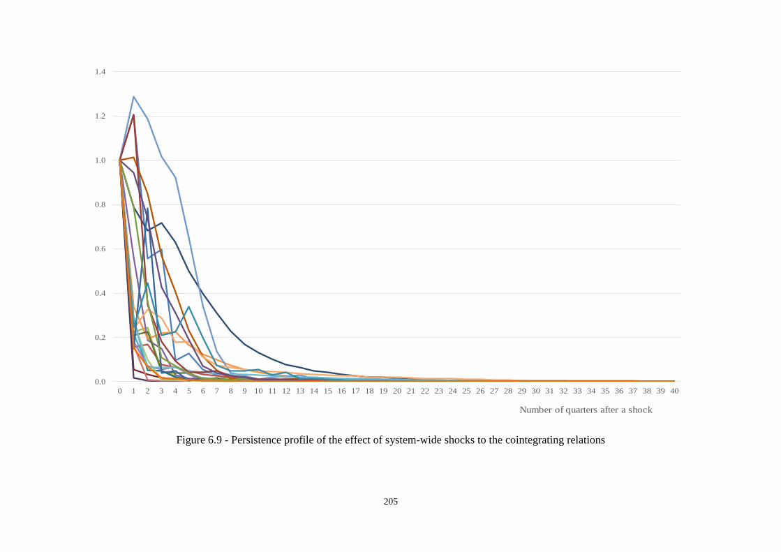
205
Figure 6.9 - Persistence profile of the effect of system-wide shocks to the cointegrating relations
0.0
0.2
0.4
0.6
0.8
1.0
1.2
1.4
0 1 2 3 4 5 6 7 8 9 10 11 12 13 14 15 16 17 18 19 20 21 22 23 24 25 26 27 28 29 30 31 32 33 34 35 36 37 38 39 40
Number of quarters after a shock

206
Table 6.10 - F-statistics for the serial correlation test of the VECMX residuals
Country Real Tourism Imports Real Tourism Exports Real Income Own price Oil Price
(lnrtim) (lnrtex) (lny) (lnp) (lnpoil)
Argentina 0.699 0.179 0.311 0.464
Australia 0.698 1.139 0.675 1.964
Austria 0.749 2.214 1.325 3.532
Brazil 0.619 1.312 1.876 0.315
Canada 1.006 0.114 3.169** 1.357
China 1.560 0.316 2.251 1.653
France 1.849 5.817*** 0.804 0.261
Germany 0.173 1.584 1.076 0.491
India 4.801*** 1.637 0.372 0.372
Italy 0.908 0.162 1.036 1.140
Japan 2.509 0.808 0.139 2.975**
Korea 0.534 1.287 0.668 2.734
Malaysia 0.884 1.003 0.323 0.212
Mexico 2.580 1.653 1.025 1.429
Netherlands 4.371*** 2.007 5.681*** 0.423
New Zealand 1.348 0.407 0.213 0.855
Norway 2.031 2.167 9.474*** 0.244
Portugal 1.323 1.009 2.441 0.532
South Africa 0.961 3.814** 2.986** 1.179
Spain 0.610 1.830 0.740 2.542
Sweden 1.119 1.193 0.250 0.771
Thailand 2.750 1.917 1.498 1.698
United Kingdom 1.428 0.425 0.193 0.127
USA 2.966** 1.048 3.361** 2.290 2.448
Note: *** and ** denote rejecting the null hypothesis of no serial correlation at the 1% and 5% significance level, respectively.
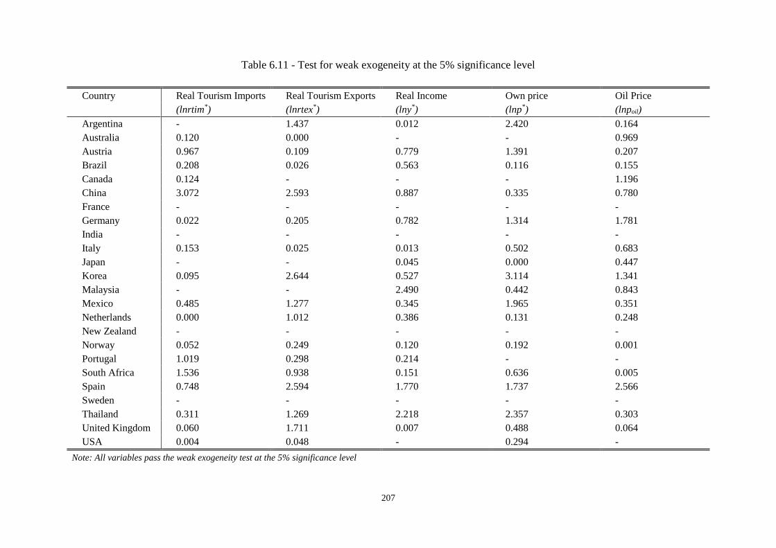
207
Table 6.11 - Test for weak exogeneity at the 5% significance level
Country Real Tourism Imports Real Tourism Exports Real Income Own price Oil Price
(lnrtim*) (lnrtex*) (lny*) (lnp*) (lnpoil)
Argentina - 1.437 0.012 2.420 0.164
Australia 0.120 0.000 - - 0.969
Austria 0.967 0.109 0.779 1.391 0.207
Brazil 0.208 0.026 0.563 0.116 0.155
Canada 0.124 - - - 1.196
China 3.072 2.593 0.887 0.335 0.780
France - - - - -
Germany 0.022 0.205 0.782 1.314 1.781
India - - - - -
Italy 0.153 0.025 0.013 0.502 0.683
Japan - - 0.045 0.000 0.447
Korea 0.095 2.644 0.527 3.114 1.341
Malaysia - - 2.490 0.442 0.843
Mexico 0.485 1.277 0.345 1.965 0.351
Netherlands 0.000 1.012 0.386 0.131 0.248
New Zealand - - - - -
Norway 0.052 0.249 0.120 0.192 0.001
Portugal 1.019 0.298 0.214 - -
South Africa 1.536 0.938 0.151 0.636 0.005
Spain 0.748 2.594 1.770 1.737 2.566
Sweden - - - - -
Thailand 0.311 1.269 2.218 2.357 0.303
United Kingdom 0.060 1.711 0.007 0.488 0.064
USA 0.004 0.048 - 0.294 -
Note: All variables pass the weak exogeneity test at the 5% significance level

208
Table 6.12 - Average pairwise cross-section correlations: variables and residuals
Real Tourism Imports (lnrtim) Real Tourism Exports (lnrtex)
Levels First
Differences
VECMX
Residuals Levels
First
Differences
VECMX
Residuals
Argentina 0.5302 0.1967 0.0403 0.5595 0.0539 -0.0064
Australia 0.6142 0.2988 0.0729 0.4261 0.1434 0.0216
Austria -0.1624 0.0267 0.0248 0.0693 0.0804 0.0385
Brazil 0.5720 0.1115 0.0280 0.6508 0.0935 0.0282
Canada 0.5508 0.2313 0.0442 0.2451 0.2197 0.0279
China 0.6160 0.0687 0.0103 0.6394 0.1542 -0.0166
France 0.5109 0.0509 -0.0567 0.3231 0.1714 -0.0249
Germany -0.0880 0.1407 0.0178 0.6584 0.1399 -0.0079
India 0.6449 0.1475 0.0110 0.6038 0.0726 0.0255
Italy 0.4284 0.1577 0.0402 -0.2965 0.1436 -0.0254
Japan -0.5215 0.2265 0.0527 0.4394 -0.0170 -0.0557
Korea 0.6101 0.1432 0.0367 0.2474 0.1133 -0.0054
Malaysia 0.6306 -0.0012 -0.0115 0.6685 0.1748 -0.0272
Mexico 0.6474 0.1488 -0.0083 0.6461 0.1494 0.0139
Netherlands -0.0499 0.0976 0.0586 0.5983 0.1584 0.0250
New Zealand 0.6279 0.1653 0.0074 0.5248 0.0390 0.0297
Norway 0.6126 0.1639 0.0364 0.4910 0.0373 0.0301
Portugal 0.5180 0.1428 -0.0103 0.6198 0.1419 0.0050
South Africa 0.6226 0.1251 0.0866 0.6465 0.0683 -0.0092
Spain 0.6533 0.2113 0.0405 0.6151 0.0902 0.0116
Sweden 0.4932 0.1891 0.0067 0.6038 0.0611 0.0540
Thailand 0.4932 0.1891 0.0434 0.6104 0.1158 0.0098
United Kingdom 0.6074 0.2085 0.0354 0.2647 0.1189 0.0061
USA 0.5623 0.3097 0.0292 0.4009 0.1511 -0.0382

209
Table 6.12 - Average pairwise cross-section correlations: variables and residuals (cont.)
Real Income (lny) Own price (lnp)
Levels First
Differences
VECMX
Residuals Levels
First
Differences
VECMX
Residuals
Argentina -0.1957 0.0676 -0.0032 -0.3605 0.0752 0.0059
Australia 0.1864 0.3773 0.0842 0.8164 0.5700 0.0774
Austria 0.0916 0.3760 0.0493 0.8090 0.5983 0.0507
Brazil -0.1166 0.1540 -0.0386 0.6345 0.3407 0.0016
Canada 0.3227 0.4681 0.1095 0.7933 0.4845 0.0471
China 0.0574 0.3010 -0.0308 0.7241 0.1784 -0.0284
France 0.0503 0.4943 0.0475 0.8037 0.6012 0.0347
Germany -0.0916 0.4123 -0.1023 0.8039 0.5979 -0.0086
India 0.0341 0.1934 -0.0005 0.7749 0.4071 -0.0116
Italy -0.0326 0.4235 0.0125 0.8074 0.5937 0.0168
Japan -0.1157 0.3812 0.0261 0.5235 0.1199 -0.1138
Korea 0.1254 0.1972 0.0378 0.6864 0.3684 -0.0213
Malaysia 0.0747 0.2613 0.0483 0.6138 0.3163 -0.0066
Mexico 0.2594 0.1709 0.0216 0.4051 0.1223 -0.0252
Netherlands 0.1686 0.4576 0.0046 0.8030 0.5928 0.0358
New Zealand 0.2798 0.3527 0.0675 0.7987 0.5398 0.0565
Norway 0.1526 0.1890 0.0037 0.8061 0.5747 0.0544
Portugal 0.1195 0.3174 0.0156 0.8012 0.5938 0.0545
South Africa 0.0559 0.4314 0.0947 0.6939 0.4270 0.0084
Spain 0.3092 0.4103 0.0535 0.8071 0.5942 0.0413
Sweden 0.3200 0.3955 -0.0034 0.7735 0.5816 -0.0228
Thailand -0.0621 0.1632 0.0268 0.7285 0.3427 0.0187
United Kingdom 0.2996 0.4642 -0.0098 0.6908 0.5308 -0.0698
USA 0.2923 0.4317 0.0536 0.6696 0.3289 0.0007
210
6.3.4 Diagnostic Tests
Diagnostic tests have been carried out onto the VECMX models’ residuals. Table 6.10
presents the test results for serial correlation of the residuals. Each column is for the
residuals from an endogenous variable’s equation in the VECMX model. In most
cases, the test is passed, meaning there is no serial correlation in most of the residuals.
Table 6.11 shows the test results for weak exogeneity, as has been described in
Section 5.2.2. Passing the weak exogeneity test means that the foreign variables 𝒙𝑖𝑡∗ in
the country-specific VECMX models do not restore the long-run cointegrating
relations that exist among domestic variables, foreign variables and global common
variables. Hence there is no ‘long-run forcing’ from 𝒙𝑖𝑡 to 𝒙𝑖𝑡∗ . The test is passed for
all the cases reported in Table 6.11. It can be spotted that some of the cases are
omitted, denoted as ‘-‘. For Argentina, Australia, Canada, Japan, Portugal, and USA,
the omitted values mean that the corresponding foreign variable has been deleted from
the country-specific VECMX models, since a preliminary estimation suggested a
violation of the weak exogeneity assumption. After taking out some foreign variables,
both the first stage VECMX models and the second stage GVAR model improved on
their performance. For France, India, New Zealand and Sweden, there are omitted
values because no cointegrating relations are found in their VECMX model (see Table
6.8) and there is no need for weak exogeneity test to address the long-run forcing
from 𝒙𝑖𝑡 to 𝒙𝑖𝑡∗ .
Following Dees, Mauro, Pesaran, and Smith (2007), in addition to the serial
correlation test and the weak exogeneity test discussed above, the average pairwise
cross-section correlations are used to see if the VECMX models are satisfactory.
Table 6.12 shows these correlations. They are essentially averaging the Pearson
correlations between a particular country and any of the other 23 countries (similar to
the ‘average’ row in Table 6.1). The idea behind Table 6.12 is to illustrate the
effectiveness of foreign variables in accounting for cross-country correlations. Note
that the column ‘levels’ indicates that, the endogenous variables for each country
almost unanimously correlate with their counterparts of other countries. The values
are generally above 0.50 for real tourism imports and real tourism exports, and even
higher (more than 0.70) for own price. But for the VECMX residuals, such
correlations are greatly reduced, thanks to the domestic variables, foreign variables

211
and global common variables in the VECMX models to account for cross-country
correlations. For all the four variables (lnrtim, lnrtex, lny, lnp), correlations of their
VECMX residuals are in many cases below 0.05 (in absolute values).
All in all, the above tests and statistics confirm that the country-specific VECMX
models are satisfactory.
6.4 Impulse Responses
Impulse response functions are well suited to track the evolution of economic
fluctuations, and are highly relevant to business cycle studies. As discussed in Section
4.6.1, in the context of globalisation, business cycles are believed to exhibit
convergence/synchronisation across countries. In the wake of a shock to China, a
major emerging economy in the world, it is expected that other major countries
experience certain degrees of fluctuations in their tourism trade. An advantage of
impulse response analysis for tourim research is that it maps out the evolution of
tourism variables after the shock. If the pattern of impulse responses of different
countries is similar, it implies that the business cycles across those countries are
synchronised. In addition, impulse response analysis is useful in illustrating how
stable a country’s economy is. If a country reacts strongly towards a shock, it means
that local businesses in that country will face great uncertainty.
In the current research, the impulse response analysis is based on hypothetical
scenarios related to changes of the Chinese economy. Specifically, it is presumed that
the Chinese economy experienced a sudden slowdown in its real GDP; another
presumption is that the Chinese currency experienced an unexpected depreciation, and
as a result a slump in its own price. Accordingly in the GVAR model, two individual
shocks are to be imposed: a negative exogenous shock to China’s real GDP variable
(lny) and a negative exogenous shock to China’s own price variable (lnp). The
impulse responses are calculated as described in Section 5.2.3. The results are
reported in the Appendices, Figure A1 to Figure A8. Among them, Figure A3, Figure
A4, Figure A7 and Figures A8 are the impulse responses of real tourism trade
variables. These figures are relevant to tourism business practitioners to gauge how
stable or how uncertain their native market will be in the face of shocks.
It should be reiterated that the shocks herein are hypothetical unexpected events. If the
events were expected, economic variables might well be adjusted beforehand since

212
economic agents (firms, consumers, and governments) could change their behaviour if
given enough time1. Therefore, impulse responses should not be seen as forecasts of
an economy. Forecasts are the expected future values of a variable based on current
realistic information, which will be factored into the economic agents’ decision in the
current period. Impulse responses are based on counterfactual scenarios and focus on
the reactions of an economy to unrealised exogenous changes.
In reporting the results from the GVAR model, an aggregation is applied to some
countries, to form a bigger region. As such, a ‘region’ in this chapter means a large
area consisting of two or more countries, rather than a small part of a country. The
aim of the aggregation is to provide a succinct presentation of the impulse responses.
The aggregation follows Table 5.2, creating such regions as South America, Asia,
Europe and Oceania. But it should be noted that the results for China, Canada,
Mexico, South Africa and the USA are individually reported. This is to highlight the
importance of China and the USA. For Canada and Mexico, it is not coherent to
combine them to form a single region of North America, in the absence of the USA.
Hence, results for Canada and Mexico are not aggregated.
6.4.1 One Negative Shock to China’s Real Income
The first counterfactual scenario is an exogenous negative shock to China’s real
income. Precisely, it is a negative shock equivalent to one standard deviation of the
error term of China’s real income equation in the GVAR model Eq. (5.18). This
means a hypothetical situation where China was experiencing a sudden decline in real
income due to exogenous reasons.
Macroeconomic variables (lny, lnp)
Figure A1 depicts the evolution of real income across countries/regions up to 40
quarters after the negative shock. For China, it results in an instant 2.7% decrease
(i.e., -0.027) in the country’s real income at the time of shock. But the decline starts to
die out quickly, amounting to roughly 0.5% in the first two years (i.e., 8 quarters) and
less than 0.4% thereafter in the long run.
1 Of course, if the expectation is formed long before the event, the economic agents are able to adjust
their optimal decisions. If the expectation is formed only well before the event, leaving the economic
agents unable to make adjustments, then the event is indeed seen as unexpected.

213
For other countries/regions, the negative shock to China generates certain impacts on
their real income. For the USA, the impact is about a 0.1% increase at the time of
shock and tends to be much lower than 0.1% thereafter. For the rest of the
countries/regions, the impacts can be a bit negative, especially in the first two years
(i.e., 8 quarters). But in the long run, the impact is only a below 0.1% increase. An
exception is Mexico, whose impulse response is more in sync with that of China, a
less than 0.2% decline in the long run.
In terms of the own price (i.e., consumer price index adjusted by a country’s exchange
rates against US dollars), the impacts of the shock are evident, mainly a drop in price
levels for all countries/regions in the short run as well as the long run. For China, its
own price level will go down by roughly 1.9%. For Asia, Europe, South Africa and
South America, the long-run impact is a decline by 1.1%, 1.9%, 2.7% and 2.3%,
respectively. For Canada, Mexico, Oceania, and USA, the long-run price drop is less
than 1%. These impulse responses are displayed in Figure A2. Synchronisation of the
impulse responses across countries/regions is observable.
Real tourism imports (lnrtim)
The evolution of real tourism imports and that of real tourism exports after the shock
to China’s real income are shown in Figure A3 and Figure A4, respectively. Overall,
the impacts mainly concentrate in the short run. Tourism trade is volatile across
different countries/regions, especially in the first three years (i.e., 12 quarters) after
the shock. However, the impacts may not necessarily last into the long run.
In the wake of a negative shock to real income, it is theoretically predicted that
outbound tourism will retract. For China, its real tourism imports will experience a
downward trend in the first two years (i.e., 8 quarters). This is in line with the finding
above that China will see a sudden drop in its real income in the very short run. After
3 years (i.e., 12 quarters), China’s real tourism imports will rebound, resulting in
roughly a 1% increase in the long run (see Figure A3). This may be due to the finding
that the own price of other countries/regions will witness varying degrees of declines
in the long run (see Figure A2), whereas China’s real income will not be much
affected in the long run (see Figure A1). The lowering of own price in other
countries/regions makes it conducive for Chinese going on outbound trips.

214
For other countries/regions, the impact of the shock tends to be discernible
particularly in the short run (see Figure A3). For the USA, it will see a slight decrease
in real tourism imports in the first year (i.e., 4 quarters) after the shock. The decrease
becomes minor thereafter. From Figure A1 and Figure A2, both the real income and
the own price of the USA are found not to be much affected by the shock to China.
The real tourism imports of Canada, Europe, Mexico, Oceania and South Africa
generally experience turbulences in the first four to eight quarters. The pattern
basically follows that of China’s impulse responses. In the long run, the real tourism
imports of these countries can return to their equilibrium level, with roughly a less
than 1% increase. For Asia, its impulse response follows that of China even more
closely, seeing a short-run decline in real tourism imports, but over the long run a 1%
increase. The much more affected area is South America, up to a 2% decline in real
tourism imports in the long run after some ups and downs in the first six quarters. The
reason could be that its own price has a 2.3% drop in the long run, and outbound
tourism is substituted away for domestic tourism.
All in all, despite the different magnitudes of long-run impacts, the short-run
fluctuations (especially in the first eight quarters) in tourism imports are generally in
sync across countries/regions.
Real tourism exports (lnrtex)
Right after the shock to China’s real income, the real tourism exports of many
countries/regions suffer from a setback in the short run. For China, its real tourism
exports will be much volatile in the first two years (i.e., 8 quarters), but the long-run
trend is towards a 2.5% increase (see Figure A4). This could be explained by the
finding that China’s own price level will drop by 1.9% in the long run after the shock,
facilitating China’s inbound tourism to attract overseas visitors.
Other countries/regions that also see certain long-run increase in real tourism exports
are South Africa (1.0%) and South America (1.7%), both of which also experience
evident own price drops (see Figure A2). For the rest of the countries/regions, i.e.,
Asia, Europe, Mexico, Oceania and the USA, their real tourism exports have notable
fluctuations in the first two years (i.e., 8 quarters), but tend to restore equilibrium in
the long run. Both Oceania and the USA will see a 0.3% drop in real tourism exports,
as their own price drops are among the least across countries/regions (see Figure A2).

215
Asia, Europe and Mexico will see an increase by 0.2% - 0.8% in the long run. For
Canada, the changes of its real tourism exports are quite stable no matter whether in
the short run or the long run, around a 0.5% increase.
Summary of findings
A negative shock to China’s real income (lny) (2.7% at the exact quarter of shock) has
relatively limited impact on the real income (lny) across all the countries/regions. But
in the long run, the impact is evident on the own price level (lnp) of almost all
countries/regions (particularly China, Asia, Europe, South Africa and South
America). In the meantime, China’s real tourism imports (lnrtim) and real tourism
exports (lnrtex) suffer from a temporary decline in the first two years (i.e., 8 quarters),
but rebound and even increase in the long run. For tourism businesses in China, it is
important to take short-run measures, such as cutting labour costs and increasing
marketing activities, in order to counter the decline in tourism demand. The tourism
trade (lnrtim, lnrtex) of other countries/regions tends to be affected basically in the
first one to two years (i.e., 4 – 8 quarters). In the long run, a notable example is South
America, whose real tourism imports (lnrtim) will go down and whose real tourism
exports (lnrtex) will rise. This should encourage local businesses in South America to
engage in catering to domestic tourists as well as overseas tourists. Synchronisation of
fluctuations across countries can be observed for the own price (lnp) constantly, and
for the real tourism imports (lnrtim) in the short run. Table 6.13 provides a brief
summary.

216
Table 6.13 - Brief summary of the findings
A negative shock to China's real income
Short run (<5 years) Long run (5-10years)
Real income China: -0.4%; Mexico: -0.2%
Own price synchronised fluctuations
China: -1.9%; Asia: -1.1%;
Europe: -1.9%; South Africa:
-2.7%; South America: -
2.3%
Real tourism imports synchronised fluctuations China: 1%; Asia: 1%; South
America: -2%
Real tourism exports Asia, Europe, Mexico, Oceania, USA:
fluctuations in the first two years
China: 2.5%; South Africa:
1%; South America: 1.7%
6.4.2 One Negative Shock to China’s Own Price
The other counterfactual scenario is an exogenous negative shock to China’s own
price. It is hypothesised to be resulting from a sudden depreciation of the Chinese
currency. Since exchange rate is a component in calculating the own price, the
negative shock is implemented on the error term of China’s own price equation in the
GVAR model Eq. (5.18). Its magnitude is one standard deviation of the error term.
In reality, the recent development of China’s currency and its consumer prices (both
elements to calculate own price) is uncertain, thus either a negative shock or a
positive shock to China’s own price could be speculated. Although the following
discussions are solely related to the consequences of a negative shock, the impulse
responses under a positive shock setting practically remain identical, with only an
opposite sign imposed on the numbers (i.e., ‘+’ becomes ‘-‘, and vice versa).
Macroeconomic variables (lny, lnp)
Figure A6 shows the development of own price level across countries/regions after
the negative shock to China. Specifically, the shock will immediately result in a

217
decline in China’s own price by about 2.0% at the exact quarter of shock. This is
similar to a 2.0% deflation in US dollar terms for China. Such deflation is rather
persistent in the long run, slightly above 1.0% even after 40 quarters.
Own price level in other countries/regions tends to decrease as well, and falls down
after the shock in the short run and the long run. The impact on USA’s own price
level is relatively small, a decline by below 0.5% in the first year (i.e., 4 quarters) and
by slightly above 0.1% in the long run. For Asia, Canada, Europe, Mexico, Oceania
and South America, their own price level will experience disturbances mainly in the
first quarter, by about -2%. Then the impact on own price quickly diminishes within
the first two years (i.e., 8 quarters) after the shock, resulting in a drop by 0.2%-0.8%
for these countries/regions in the long run. An exception is Oceania, which will see a
price increase by roughly 0.5%. The only country that will witness a deeper long-run
impact on its own price is South Africa. It will have a decline in own price by
approximately 1.5%. In general, co-movements of the impulse responses are present
across countries/regions.
In terms of real income (see Figure A5), the shock tends not to create much impact,
no matter whether in the short run or the long run. For China, Asia, Mexico and South
America, the long-run impact on their real income is negative, at -0.1% for China and
far smaller than -0.1% for the others. For Canada, Oceania, South Africa and the
USA, the long-run impact is positive, at 0.2% for Oceania and again far smaller than
0.1% for the rest. For Europe, the shock is hardly felt in terms of real income and the
impact is almost zero. It is, however, difficult to provide definitive explanations as to
how real income should react in the long run alongside a relatively mild drop in the
price level. After all, changes in the price level have implications on the wages of
labour (hence their disposable income), the private and government consumptions, the
cost of capital investments, the expenses of technological developments, and net
exports, all of which may contribute to a new market clearing level of real income in
the long run. Hence, the real income level across countries/regions may well react to
the shock differently in the long run.
Real tourism imports (lnrtim)
The shock to China’s own price generally has mild impacts on real tourism imports
across countries/regions. Figure A7 illustrates the impulse responses. For China, its

218
real tourism imports will experience some downward pressure, declining by 2.1% at
the time of shock. Thereafter, the decline becomes stable, at around 1% in the long
run. This could be associated with a similar pattern of impulse responses in China’s
own price (see Figure A6). As discussed above, China’s own price level will have a
roughly 1.0% drop in the long run, while the own price of other countries/regions
(i.e., the potential outbound destinations) is only slightly changed. Hence, there could
be a small decline in China’s outbound tourism, in favour of domestic tourism
instead.
For the other countries/regions, their real tourism imports are mildly affected. In the
long run. Asia, Oceania and USA will see slight decline in terms of their outbound
tourism, at 0.97%, 0.59% and 0.59% respectively after 40 quarters. For Canada,
Europe, Mexico and South Africa, the changes in real tourism imports mainly take
place in the first year (i.e., 4 quarters) after the shock. Thereafter, the impact is a
relatively small increase in real tourism imports, at roughly 0.2% or even much lower.
The only region that may see a large long-lasting impact is South America. Its real
tourism imports are expected to go down by 1.6% in the long run, a likely reaction to
the decline in both its real income (less budget to spend) and its own price level
(cheaper for domestic trips).
Real tourism exports (lnrtex)
Similar to real tourism imports, by and large the real tourism exports do not suffer
extensively from the shock to China’s own price. Figure A8 outlines the impulse
responses across countries/regions. For China, its real tourism exports will experience
some ups and downs in the first year (i.e., 4 quarters), roughly 2%-3% in absolute
values. Thereafter, China’s real tourism exports will decline by about 0.2% in the long
run. The reason behind such decline is not obvious. As discussed above, China’s own
price will have a long-term drop at around 1%-2%. In the meantime, the own price
level of most other countries/regions will see a smaller decline (by about 1%) in the
short run. Hence, the pattern of China’s real tourism exports suggests that, China is
not particularly effective in taking advantage of the own price drop in order to entice
inbound tourists. As will be discussed immediately, some other countries/regions will
see a long-run increase in their real tourism exports. These are the countries/regions
that are more successful than China in attracting international tourists.
219
A long-run drop in real tourism exports is seen in Asia, Oceania and USA, at about
0.5%, 0.9% and 0.7% respectively. For Canada and Europe, their real tourism exports
are generally calm and stable in both the short run and the long run, with an increase
by 0.03% and 0.08% after 40 quarters. In comparison, the real tourism exports of
Mexico, South Africa and South America are more volatile in the first year (i.e., 4
quarters) after the shock. Fluctuations can be up to ±3% during this period. In the long
run, the impact on real tourism exports is roughly a 0.3%-0.6% increase. In the short
run, certain level of synchronisation can be widely spotted between Canada, China,
Europe, Mexico and South America.
Summary of findings
Overall, the impacts of a shock to China’s own price level (lnp) are smaller than those
of a shock to China’s real income (lny). The real income (lny) across countries/regions
is only slightly changed, irrespective of the horizon. The changes in own price level
(lnp) are particularly evident in the first two years for most of the countries/regions. In
the long run, only China and South Africa will see noticeable decline in their own
prices (lnp). In terms of tourism trade (lnrtim, lnrtex), China will see long-lasting
contraction in both tourism imports (-1%) and tourism exports (-0.2%). So travel
agents arranging overseas trips for Chinese tourists have to make effort to counter the
decline of outgoing tourism demand in the long run. The other countries/regions will
however experience fluctuations in the very short run. An exception is South
America, whose real tourism imports (lnrtim) will decrease even in the long run.
Synchronisation of fluctuations are widely observed across most countries/regions for
own price level (lnp) and real tourism exports (lnrtex). Table 6.14 presents a brief
summary.
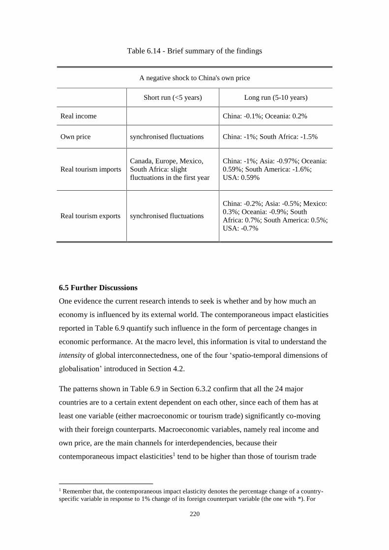
220
Table 6.14 - Brief summary of the findings
A negative shock to China's own price
Short run (<5 years) Long run (5-10 years)
Real income China: -0.1%; Oceania: 0.2%
Own price synchronised fluctuations China: -1%; South Africa: -1.5%
Real tourism imports
Canada, Europe, Mexico,
South Africa: slight
fluctuations in the first year
China: -1%; Asia: -0.97%; Oceania:
0.59%; South America: -1.6%;
USA: 0.59%
Real tourism exports synchronised fluctuations
China: -0.2%; Asia: -0.5%; Mexico:
0.3%; Oceania: -0.9%; South
Africa: 0.7%; South America: 0.5%;
USA: -0.7%
6.5 Further Discussions
One evidence the current research intends to seek is whether and by how much an
economy is influenced by its external world. The contemporaneous impact elasticities
reported in Table 6.9 quantify such influence in the form of percentage changes in
economic performance. At the macro level, this information is vital to understand the
intensity of global interconnectedness, one of the four ‘spatio-temporal dimensions of
globalisation’ introduced in Section 4.2.
The patterns shown in Table 6.9 in Section 6.3.2 confirm that all the 24 major
countries are to a certain extent dependent on each other, since each of them has at
least one variable (either macroeconomic or tourism trade) significantly co-moving
with their foreign counterparts. Macroeconomic variables, namely real income and
own price, are the main channels for interdependencies, because their
contemporaneous impact elasticities1 tend to be higher than those of tourism trade
1 Remember that, the contemporaneous impact elasticity denotes the percentage change of a country-
specific variable in response to 1% change of its foreign counterpart variable (the one with *). For

221
variables. The magnitude of elasticities for macroeconomic variables generally stands
at between 0.9-1.5, quite elastic. The interdependencies between tourism trade
variables are admittedly less impressive. Still, over half of the 24 countries see their
inbound or outbound tourism demand co-move with their foreign counterparts, though
the magnitude of elasticities usually falls in between 0.5-0.8, only moderate and not
so elastic. As suggested in Section 6.3.2, this is possibly because tourism demand is
also affected by country-specific non-economic factors, which render a country’s
tourism demand less susceptible to external economic changes alone.
Another pattern from Table 6.9 that might be of interest is whether there is a divide
between countries in terms of their magnitude of contemporaneous impact elasticities.
One divide could be emerging economies versus developed economies. However, the
pattern is not very outstanding. The magnitude of contemporaneous impact
elasticities, if statistically significant, is not higher for developed economies than for
emerging economies, nor the other way round. The only pattern, as hinted in Section
6.3.2, is that European countries tend to have more variables associated with
statistically significant contemporaneous impact elasticities. This may be explained by
the fact that, of the 24 countries in the current research, ten are European countries,
which are well connected to each other economically.
If the contemporaneous impact elasticities in Table 6.9 take care of the intensity
dimension of globalisation, then the impulse response analysis in Section 6.4 is an
attempt to assess the impact propensity of global interconnectedness, another ‘spatio-
temporal dimension of globalisation’ (see Section 4.2). The impulse responses
illustrate the developments of different variables across a number of major countries
in the wake of shocks. China, as an important emerging economy, is chosen to be
where the shocks originate. The shocks are expected to have global impacts.
Table 6.13 and Table 6.14 summarise the findings from the impulse response
analysis. Between the two negative shocks, a shock to China’s real income tends to
have deeper impacts on other countries/regions. The long-run changes of a
country’s/region’s variables (real income, own price, real tourism imports, and real
tourism exports) are rougly 2%-3% (in absolute values). But a shock to China’s own
example, how many percentage China’s real income will change, if the weighted average of other
countries’ real income rises up by 1%.

222
price tends to create wider impacts in terms of geography. More countries/regions are
affected even in the long run.
Between the variables, the real income level across countries/regions is the least to be
affected by either shock. The own price level across countries/regions will, however,
experience changes in both the short run and the long run. For the real tourism
imports and real tourism exports, short-run flucutations are widely observed after
either shock, and in the long run many countries/regions still see a slight decline.
Between the countries/regions, the developed countries/regions, such as Europe,
Canada and the USA, are generally affected only in the short run. Synchronised
fluctuations in terms of own price level and real tourism demand are found after both
shocks. However, in the long run basically it is the developing countries/regions (such
as South Africa and South America) that suffer from continuous impacts. This finding
to some extent resonates with that of Kose, Otrok, and Prasad (2012), who find a
substantial convergence of business cycles among emerging market economies
alongside a convergence among industrial economies. Asia, the region where China
situates and can be seen as a short-haul market to China, is also among the regions
that see long-run impacts by the shocks. As shown in Table 4.2 and Table 4.3, China
interacts intensively with the other Asian countries in terms of tourism trade.
Overall, Table 6.13 and Table 6.14 (together with the impulse responses charts Figure
A1 to Figure A8) provide another evidence of interdependencies between tourism
countries. That is, in the short run, the fluctuations of own price variable and tourism
trade variables across major countries in the world are somewhat in sync; but of
course, in the long run, China’s unexpected economic changes tend to have persistent
influence over other developing countries and those that are geographically close to
China, rather than developed countries in the West.
Admittedly, the estimation results from the GVAR approach outline only part of the
temporal-spatial dimensions of globalisation. Nevertheless, from an economic
perspective, the above evidence is able to demonstrate that, rather than a perfectly
interconnected world where all economies co-move strongly, the economy and the
international tourism sector of major countries experience synchronised movements
mainly in the short run. But in the long run, the tendency becomes evident that the

223
countries in similar stage of development (developing countries) and in proximate
region are more in sync.
6.6 Practical Implications
Modelling the interdependencies between tourism demand provides information about
the reaction of a country’s international tourism sector towards changes in other
countries. From a practical point of view, the economic performance of a country’s
international tourism sector, in terms of tourism imports and tourism exports, is
inevitabley influenced by the country’s external economic climate. In the same vein,
at the micro level, the financial performance of tourism businesses is reliant on the
macroeconomic climate both at home and abroad.
The GVAR model quantifies the impacts of external influence, in the form of
contemporaneous impact elasticities and impulse responses towards exogenous
shocks. This quantitative information is particularly relevant to macroeconomic
analysis for tourism authorities as well as multi-national corporations in tourism and
hospitality, especially when they are developing business strategy and making
decisions about procurement and employment.
6.6.1 Use of the Results
With regard to the contemporaneous impact elasticities reported in Table 6.9, the
higher the values are, the deeper a country’s intenraiotnal tourism sector is integrated
with the world and hence the more vulnerable to external changes. For a country
where international tourism is a major industry, higher elasticity values mean that the
country will face higher uncertainty (due to fluctuations) of its economic performance
in times of turbulence. Such uncertainty is a double-edged sword. On the one hand, it
means a higher growth opportunity for the countries with higher elasticities than for
those with lower elasticities, if the world is experiencing advances (for example,
technological progress). On the other hand, it means deeper recession for the
particular country, if adverse events (for example, economic crisis, political unrests)
take place around the world. For a country with lower elasticities, it can expect a
relatively stable economic performance in its international tourism sector.
Hence, to some extent the contemporaneous impact elasticities reflect the
competitiveness of a country’s international tourism sector. An ideally-managed
destination should aim to adjust its tourism sector between low elasticities and high
224
elasticities across different stages of business cycle, such that in times of adversity it
is less vulnerable (low elasticities), but in times of booming it can capture high
economic yield (high elasticities).
At the corporate level, tourism businesses can use the contemporaneous impact
elasticities as general indicators of variability of their local economies, when they are
planning their future activities such as procurement and employment. For example, in
Table 6.9, column Real Tourism Exports, the impact elasticities for France and Italy
are 0.752 and 0.841 respectively, while for Portugal and Spain 0.548 and 0.373. These
stastistics mean that if the overall inbound tourism around the world increases by 1%,
then the inbound tourism of France and Italy will increase by a larger degree than
Portugal and Spain will. As a result, tourism-related companies in France and Italy
generally face a more variable inbound tourism demand time and time again, which in
turn requires the companies to make better coordination with their suppliers and make
better employment plan.
The impulse responses reported in Figure A1 to Figure A8 of the Appendices show
how the performance of a country’s international tourism sector will evolve, in the
wake of exogenous and unexpected events in other parts of the world. Specifically,
after the shocks to China, short-run synchronised fluctuations are observed across
both developing countries and developed countries, whereas long-run impacts are
evident for developing countries and for China’s short-haul markets. Hence, for other
developing countries and the Asian countries, the development of the Chinese
economy is particularly relevant to maintaining stability in their international tourism
sector as well as their local economies. For developed countries, although no long-run
impacts are expected, the short-run fluctuations resulting from a shock to China may
not be desirable to tourism businesses.
Indeed, businesses in both developing countries and developed countries can make
use of the information on the timefrome after which their local economies restore
equilibrium. For example, if a country’s real tourism exports are expected to face
fluctuations in the first two years (i.e.,8 quarters) after a shock to China, it is
necessary for the local businesses (tourism-related companies) to allow for sufficient
flexibility in their production (e.g., flexibility in employment arrangement) to cope

225
with the fluctuations of inbound tourism demand for a two-year period. Such
flexibility should be factored into the companies’ business strategies.
It should be noted that, impulse responses are essentially different from the forecasts
in many tourism demand studies. On the one hand, tourism demand forecasts assume
that the historical trends of variables can be maintained, and future values of tourism
demand are only continuations of existing trends. On the other hand, impulse
responses assume a sudden change to historical trends, and such ‘new information’
will be embedded in ‘future’ values. Given that the timing of shocks cannot be known
beforehand, the impulse response analysis only provides counterfactual scenarios,
rather than realistic forecasts. Nevertheless, based on the impulse responses, tourism
businesses can establish contingency plans under the counterfactual scenarios.
In short, it is not appropriate to compare the impulse responses with any tourism
demand forecasts published in other studies. The impulse responses are useful to
gauge how well or how badly a country copes with uncertainty. Apparently, with the
GVAR model, any other shocks (i.e., other counterfactual scenarios) can also be
considered for impulse response analysis.
6.6.2 Implications for the Major Countries
Based on the above discussions, country/region-specific implications are drawn as
follows. It should be reiterated that China and the USA are reported as individual
countries for the impulse response analysis in Section 6.4. Hence, both countries
continue to be discussed individually in this current section.
China
China’s real income and own price are mildly affected by its foreign counterparts, but
its tourism trade is not significantly affected. These results suggest that the Chinese
economy (including its internatioan tourism sector) should be rather stable, in the
wake of external turbulences. But facing the negative shocks to its own economy (real
income and own price level), China is expected to suffer from some short-run
fluctuations as well as long-run impacts. Tourism businesses should be prepared for
considerable ups and downs during the first two years after a shock. Thereafter,
tourism businesses continue to face a change in the level of tourism imports and
tourism exports, which should be factored into their long-term business strategies.
226
Asia
The other countries in Asia (especially India and Thailand) tend to have higher
contemporaneous impact elasticities than China does, indicating their higher levels of
dependency on external environment. Seen as a neighbouring area to China, Asia is
expected to witness notable changes after the shocks to the Chinese economy. The
first two years are important to tourism businesses in the Asian countries because of
the fluctuations in international tourism demand, especially after a shock to China’s
real income. As with their Chinese counterparts, tourism businesses in other Asian
countries should expect long-lasting changes in the level of tourism imports and
tourism exports.
Europe
European countries generally have more contemporaneous impact elasticities that are
significant and elastic than other countries, meaning that their economies could face
high volatility if the external environment changes. As analysed in the previous
sections, this pattern might be due to the fact that many European countries are
chosen in the GVAR model and they are well interconnected to each other. Seen as a
long-haul market to China, Europe appears to cope with the shocks in China fairly
well. For tourism businesses, the window of uncertainty is the first one to two years
after the shocks, during which small fluctuations can be observed. In the long-run, the
impacts are not so noticeable.
Oceania
Both Australia and New Zealand’s tourism trades are not very sensitive to external
changes, according to their contemporaneous impact elasticities. But New Zealand’s
macroeconomic variables are quite elastic. Though still within the Asia-Pacific area,
both Australia and New Zealand are a bit farther away from China than most of the
Asian countries are. The impacts of shocks in China tend not to be long-lived, with
the first two years (especially after the one to China’s real income) being a bit volatile
for tourism businesses in Oceania.
South Africa

227
Real income and especially own price are two main channels through which South
Africa is affected by its external environment, whereas its tourism trade is inelastic.
The negative shocks in China result in moderate fluctuations for South Africa’s
tourism trade in the first one to two years. In the long run, since the own price level in
South Africa is going to drop remarkably, the level of tourim exports is expected to
rise quite noticeably.
South America
Compared with other countries, Argentina and Brazil are evidently dependent on the
external world. But the magnitude of the contemporaneous impact elasticities is
average compared to other countries/regions. In response to the shocks in China,
tourism businesses in South America should be warned against strong fluctuations in
international tourism demand especially in the first year. Thereafter, tourism
businesses should be aware of some long-run changes in tourism trade. Under the two
shocks discussed in Section 6.4, South America generally sees an increase in tourism
exports along with a decrease in tourism imports. As explained, this pattern could be
due to the fact that the own price level falls down in the long run, making the region
price-wise particularly attractive to incoming tourists.
North America: Canada
Only the contemporaneous impact elasticity of real tourism imports is measured for
Canada. It is statistically significant, but not elastic. Compared with all other countries
studied, Canada is the least affected by the shocks in China. Short-run fluctuations of
Canada’s tourism trade is observed mainly in the first two years after the shocks.
North America: Mexico
The real income of Mexico is greatly influenced by external changes. Hence, a shock
to China’s real income causes quite noticeable short-run fluctuations in Mexico’s real
income. Overall, in the wake of shocks in China, tourism businesses in Mexico should
pay more attention to short-run changes in international tourism demand during the
first two years. In the long-run, the international tourism demand is not going to
change dramatically.
North America: USA

228
The contemporaneous impact elasticites of the USA are not very high, even though
they are found statistically significant. Economically, the USA is more likely to exert
influence over other countries, while it is not necessarily affected by its external
environment to a great extent. A shock to China’s real income causes remarkable
flucations in the USA’s tourism trade especially in the first year. But in the long run,
tourism trade does not change that much. In comparison, a shock to China’s own price
has quite consistent impacts on the USA’s tourism trade. Tourism businesses should
expect small changes in the level of tourism demand right after this shock.
6.7 Conclusion
Overall, the GVAR model is satisfactory in terms of passing the diagnostic tests and
generating credible empirical results. Particularly, the core assumption of weak
exogeneity is met in the country-specific VECMX models.
Correlations of tourism imports and those of tourism exports are found across
countries, implying the presence of interdependencies. The GVAR model provides a
rigorous framework to quantify such relations.
Contemporaneous impact elasticities are thus derived to measure how much a country
will change in reaction to changes in foreign countries. It is confirmed that all of the
24 major countries sampled in the current research, to various extents, see their
international tourism demand as well as their local economies integrated with their
foreign counterparts.
In addition, impulse responses are simulated to see how negative shocks to China’s
economy will result in changes in other countries’ international tourism demand as
well as their local economies. Generally speaking, the shocks will cause short-run
fluctuations in own price level and real tourism trade (imports and exports) across
both developing countries and developed countries. But in the long run, the impacts
are more likely to remain for developing countries plus China’s neighbouring
countries, rather than for developed countries in the West.
The above results justify the importance for tourism businesses and policy makers to
be vigilant to events in other parts of the world, since businesses are now operating in
an interdependent environment.
229
Chapter 7. Conclusions
7.1 Introduction
This current research identifies some research gaps and proposes adopting a new
modelling approach to study international tourism demand. In brief, the new approach
has generated satisfactory estimation results and is able to answer the research
questions set out at the beginning of the research. Practical implications are drawn in
relation to how tourism policy makers and business practitioners can make use of the
empirical results.
The following sections summarise the main findings from previous chapters, with a
view to articulating the theoretical and practical contributions of the current research.
Furthermore, the limitations of the GVAR approach are discussed. To conclude the
current research, future research directions are identified.
7.2 Summary of the Findings
The current research is set out to study economic interdependencies of international
tourism demand across major countries in the world. Globalisation provides the
backdrop to understand the research questions.
Through literature review, it is found that there is a gap between the capabilities of
existing tourism demand models and the current economic reality. Economic
activities of different countries are increasingly interconnected. In the international
tourism sector, tourism destinations are not only affected by the economic fluctuations
in their inbound tourists’ home countries, but also play a role in transmitting the
business cycles to other countries. As a result, co-movements of business cycles of
international tourism demand are expected to be observed, an example being the
recent global recession in 2008-2009. In such a globalising setting, gauging the
impacts of shocks in a major country, such as China, is of particular relevance to
tourism businesses in any other countries. However, the independent nature of cross-
country relations has not been properly accounted for in most of existing tourism
demand models.
In order to fill this research gap, the current research develops a tourism demand
model using an innovative approach, called the global vector autoregressive (GVAR)
approach. The current research considers tourism trade, i.e., tourism imports and
tourism exports, as the measure of tourism demand. Two economic factors, namely a

230
country’s real income and a country’s own price (i.e., exchange-rate-adjused
consumer price index), are identified as the determinants of international tourism
demand, and these two factors also exhibit cross-country linkages. The oil price is
regarded as an observable global common factor that influences the internatioan
tourism demand across countries.
Overall, the GVAR approach has generated satisfactory estimation results, from the
standpoint of statistical significance and diagnostic test results. Results show that all
the 24 major countries, to different extents, see their tourism trade as well as their
local economies move alongside their foreign counterparts. Besides, impulse
responses are simulated to see how negative shocks to the Chinese economy will
affect other countries. It is found that synchronised short-run fluctuations of the own
price and of the real tourism trade across almost all the 24 countries are observed. But
in the long run, the impacts tend to be deeper for developing countries as well as
China’s neighbouring countries, than for developed countries in the West.
In meeting the research objectives, the current research attempts to contribute to the
knowledge on tourism demand on both the theoretical front and the practical front:
1. It studies the endogeneity issue in tourism demand models and interprets the
issue in a practical context;
2. It reviews the economic interdependencies of tourism demand across different
countries, and it provides an outline for studying economic globalisation in the
context of tourism;
3. It developes a tourism demand model based on an innovative approach, which
is able to overcome the endogeneity issue;
4. The empirical results are helpful to measure the intensity and the impact
propensity of economic interdependencies;
5. The empirical results are useful for tourism policy makers and business
practitioners in different countries when they conduct macroeconomic
analysis.
7.3 Limitations of the Current Research
As with any other studies, the current research is not exempt from limitations. They
are down to the data quality and are also inherent to the model, which albeit is a new
approach but still requires further developments:

231
1. There could be more countries in the data set. The more countries included,
the more representive the data set becomes. One solution is to aggregate all the
countries that are not listed in the data set as an imaginary country called ‘Rest
of the World (ROW)’. However, this solution is vulnerable. For example,
calculating the total exports of ROW means all the intra-regional exports and
imports have to be cancelled out, leaving in only the trade with the countries
outside ROW. This is a cumbersome process, and it faces a great
unavailability of bilateral trade data. Hence, a fundamental issue remains that
the availability of data varies greatly across countries and over time. A
tradeoff has to be made between the number of countries and the amount of
available data.
2. The econometric model used in the current research only explicitly considers
economic factors. The model basically is only capable of accounting for the
economic aspects of interdependencies, since it is understandably very
difficult and not practical to quantify non-economic factors. Essentially, other
studies using econometric methods encounter similar limitations. The current
research manages to study the economic aspects of interdepencies in a
coherent manner, as the theories underlying the research topic are
systematically reviewed, and the econometric model is constructed in line with
economic theories as well as previous empirical evidence. In addition, with
regard to the model, while it is sensible to argue that economic factors are
interdependent across countries, it might not be reasonable to justify that non-
economic factors will also co-move in a short- to medium-term period. Hence,
it is not appropriate to include both economic factors and non-economic
factors within the same econometric model, even if there were some ways to
measure the non-economic factors in numerical terms. The non-economic
aspects of interdependencies may be better studied on a relatively qualitative
basis, which deserve to be a separate research.
3. The empirical results concern about each country’s overall tourism trade,
without further splits into their trading partners. For example, after a shock,
China’s total outbound tourism is expected to increase by 1% in the long run.
There is no information about how this increase will be distributed across the
destinations. This limitation is down to the use of a country’s overall tourism
trade figures, rather than bilateral tourism figures. The model itself does not

232
necessarily measure the co-movements between specific origin-destination
pairs. For n countries, there will be n·(n-1) pairs; for 24 countries, there will be
552 pairs. It is not viable to model them altogether. Nevertheless, the model
works well with the overall trade figures, and the endogeneity between these
figures are well accounted for.
All in all, the current research faces issues that could also arise in other econometric
models, basically due to the unavailability of data and the choice of specific variables.
While the latter might be (partly) accommodated through using other types of models,
the former is somewhat at the mercy of data producers.
7.4 Recommendations for Future Research
The current research is an initial attempt to approach a topic using a rigorous,
quantitative method. Future research on interdependencies can aim to explore further
developments of the GVAR approach, and/or in new contexts:
1. The GVAR approach can be applied to different sample periods. The results
such as contemporaneous impact elasticities can then be compared across
different periods. Implications can be drawn with regard to the evolution of
interdependencies over time. This reflects the idea that the degree of
globalisation is changing, as presented in Section 4.2. Although such an idea
may not prove to be correct, attempts to map out the different levels of
interdependencies over time will be helpful for theoretical discussions. A
major consideration is the length of sample period, which has to be
sufficiently long. Gathering sufficient data may be a pressure.
2. The GVAR approach may be used in conjunction with other econometric
techniques, such as time-varying-parameters (TVP) and Bayesian statistics.
The idea of TVP is similar to the first recommendation, which is to capture the
variations of elasticities over time. Bayesian VAR is an increasingly popular
model that provides an alternative way to deal with the overfitting issue. The
GVAR approach can be further developed with the ‘new’ techniques. New
dimensions will be brought into the estimation process. Hence, additional
information can be drawn accordingly.
3. The GVAR approach is also fit for other contexts. Even though it was initially
intended for modelling global interdependencies, the approach may be applied

233
to a regional context that consists of active intra-regional tourism, such as the
European Union, China and the USA; it may also be applied to explore the
interdependencies between tourism and other sectors in an economy.
The value of GVAR approach is that it clears one important issue in existing tourism
demand models, and hence allows for many new opportunities for tourism economics
research.
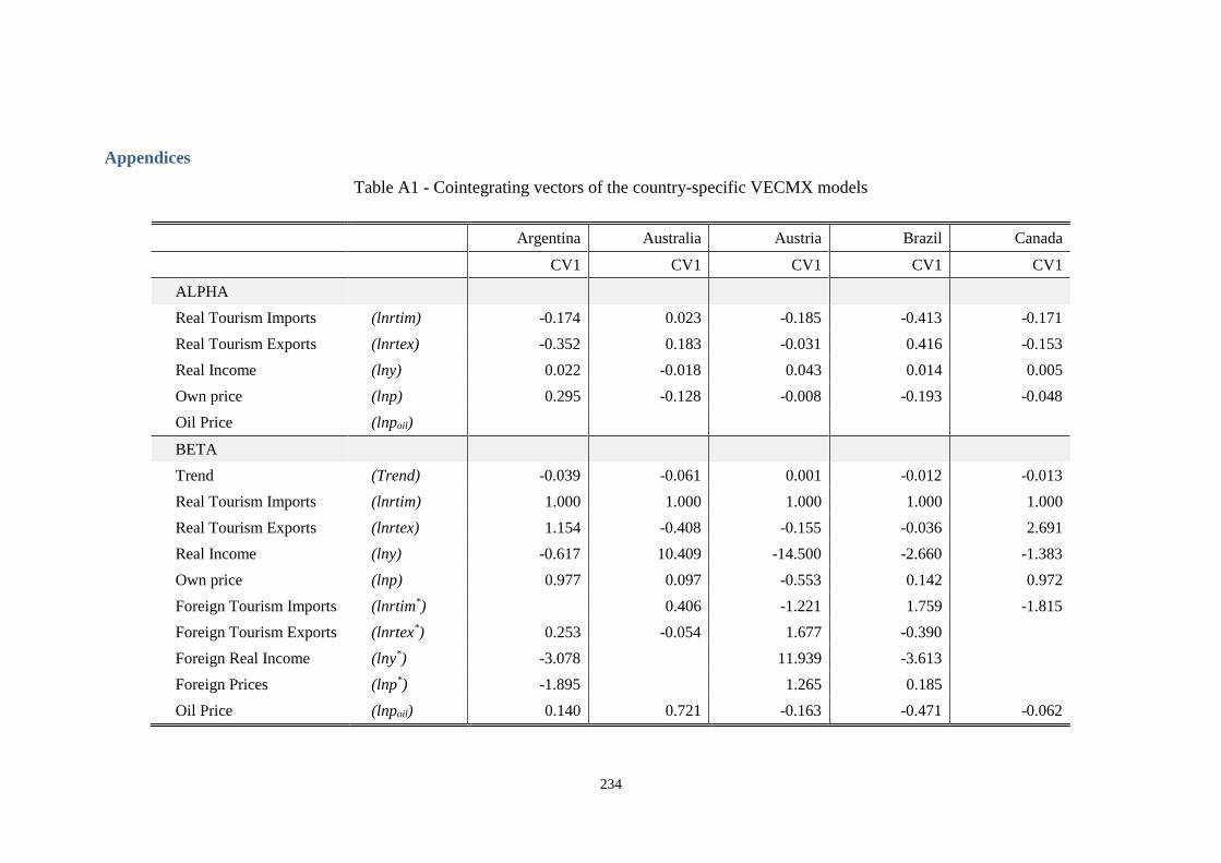
234
Appendices
Table A1 - Cointegrating vectors of the country-specific VECMX models
Argentina Australia Austria Brazil Canada
CV1 CV1 CV1 CV1 CV1
ALPHA
Real Tourism Imports (lnrtim) -0.174 0.023 -0.185 -0.413 -0.171
Real Tourism Exports (lnrtex) -0.352 0.183 -0.031 0.416 -0.153
Real Income (lny) 0.022 -0.018 0.043 0.014 0.005
Own price (lnp) 0.295 -0.128 -0.008 -0.193 -0.048
Oil Price (lnpoil)
BETA
Trend (Trend) -0.039 -0.061 0.001 -0.012 -0.013
Real Tourism Imports (lnrtim) 1.000 1.000 1.000 1.000 1.000
Real Tourism Exports (lnrtex) 1.154 -0.408 -0.155 -0.036 2.691
Real Income (lny) -0.617 10.409 -14.500 -2.660 -1.383
Own price (lnp) 0.977 0.097 -0.553 0.142 0.972
Foreign Tourism Imports (lnrtim*) 0.406 -1.221 1.759 -1.815
Foreign Tourism Exports (lnrtex*) 0.253 -0.054 1.677 -0.390
Foreign Real Income (lny*) -3.078 11.939 -3.613
Foreign Prices (lnp*) -1.895 1.265 0.185
Oil Price (lnpoil) 0.140 0.721 -0.163 -0.471 -0.062
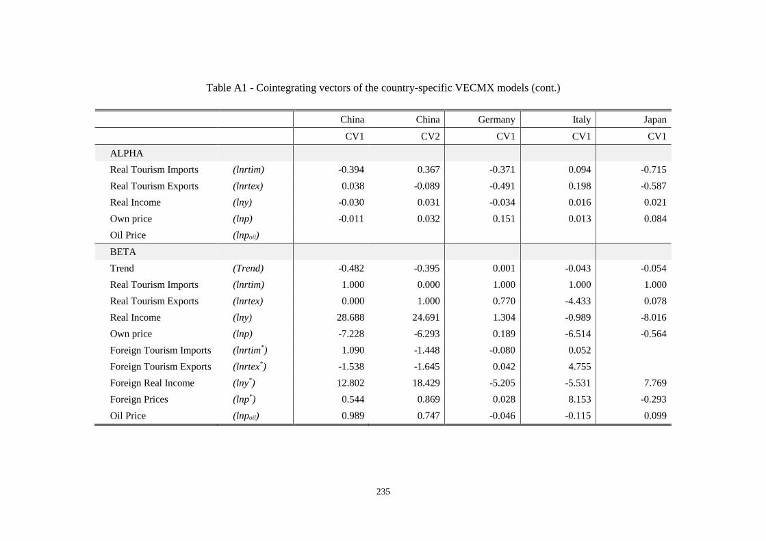
235
Table A1 - Cointegrating vectors of the country-specific VECMX models (cont.)
China China Germany Italy Japan
CV1 CV2 CV1 CV1 CV1
ALPHA
Real Tourism Imports (lnrtim) -0.394 0.367 -0.371 0.094 -0.715
Real Tourism Exports (lnrtex) 0.038 -0.089 -0.491 0.198 -0.587
Real Income (lny) -0.030 0.031 -0.034 0.016 0.021
Own price (lnp) -0.011 0.032 0.151 0.013 0.084
Oil Price (lnpoil)
BETA
Trend (Trend) -0.482 -0.395 0.001 -0.043 -0.054
Real Tourism Imports (lnrtim) 1.000 0.000 1.000 1.000 1.000
Real Tourism Exports (lnrtex) 0.000 1.000 0.770 -4.433 0.078
Real Income (lny) 28.688 24.691 1.304 -0.989 -8.016
Own price (lnp) -7.228 -6.293 0.189 -6.514 -0.564
Foreign Tourism Imports (lnrtim*) 1.090 -1.448 -0.080 0.052
Foreign Tourism Exports (lnrtex*) -1.538 -1.645 0.042 4.755
Foreign Real Income (lny*) 12.802 18.429 -5.205 -5.531 7.769
Foreign Prices (lnp*) 0.544 0.869 0.028 8.153 -0.293
Oil Price (lnpoil) 0.989 0.747 -0.046 -0.115 0.099

236
Table A1 - Cointegrating vectors of the country-specific VECMX models (cont.)
Korea Malaysia Malaysia Mexico Netherlands
CV1 CV1 CV2 CV1 CV1
ALPHA
Real Tourism Imports (lnrtim) -0.079 -0.142 -0.001 0.089 -0.188
Real Tourism Exports (lnrtex) -0.121 0.797 -0.613 0.225 0.303
Real Income (lny) -0.008 -0.026 0.031 0.173 -0.001
Own price (lnp) -0.020 0.094 -0.042 -0.101 -0.036
Oil Price (lnpoil)
BETA
Trend (Trend) -0.073 0.009 0.020 -0.039 0.015
Real Tourism Imports (lnrtim) 1.000 1.000 0.000 1.000 1.000
Real Tourism Exports (lnrtex) 3.205 0.000 1.000 -0.913 -1.593
Real Income (lny) 5.766 -6.787 -11.407 -7.756 -3.516
Own price (lnp) 5.699 1.521 3.158 0.824 2.292
Foreign Tourism Imports (lnrtim*) -4.192 -0.158 -2.321
Foreign Tourism Exports (lnrtex*) 2.248 0.747 1.382
Foreign Real Income (lny*) 2.011 -12.818 -16.622 8.763 10.066
Foreign Prices (lnp*) -2.655 1.675 2.801 4.567 -3.465
Oil Price (lnpoil) -0.711 -0.017 -0.251 -0.022 0.193

237
Table A1 - Cointegrating vectors of the country-specific VECMX models (cont.)
Norway Portugal Portugal South Africa Spain
CV1 CV1 CV2 CV1 CV1
ALPHA
Real Tourism Imports (lnrtim) 0.026 -0.133 0.200 -0.676 -0.160
Real Tourism Exports (lnrtex) 0.060 0.201 -0.365 -0.479 0.087
Real Income (lny) 0.007 0.059 0.012 -0.011 0.057
Own price (lnp) 0.001 0.074 -0.309 0.095 0.046
Oil Price (lnpoil)
BETA
Trend (Trend) -0.001 -0.009 -0.020 -0.023 -0.003
Real Tourism Imports (lnrtim) 1.000 1.000 0.000 1.000 1.000
Real Tourism Exports (lnrtex) -14.836 0.000 1.000 0.218 -0.547
Real Income (lny) -54.113 -2.148 -0.033 1.118 -4.067
Own price (lnp) -15.690 -0.127 0.523 0.602 2.104
Foreign Tourism Imports (lnrtim*) -6.099 -2.344 -0.004 1.608 0.777
Foreign Tourism Exports (lnrtex*) 10.733 1.806 0.814 -1.772 -0.660
Foreign Real Income (lny*) 39.837 2.208 -4.403 -1.938 6.896
Foreign Prices (lnp*) 16.996 -0.581 -2.554
Oil Price (lnpoil) 0.772 -0.145 -0.140
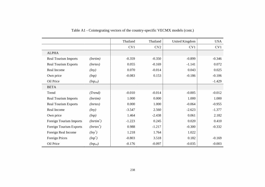
238
Table A1 - Cointegrating vectors of the country-specific VECMX models (cont.)
Thailand Thailand United Kingdom USA
CV1 CV2 CV1 CV1
ALPHA
Real Tourism Imports (lnrtim) -0.359 -0.350 -0.899 -0.346
Real Tourism Exports (lnrtex) 0.055 -0.169 -1.141 0.072
Real Income (lny) 0.070 -0.014 0.043 0.025
Own price (lnp) -0.083 0.153 -0.186 -0.106
Oil Price (lnpoil) -1.429
BETA
Trend (Trend) -0.010 -0.014 -0.005 -0.012
Real Tourism Imports (lnrtim) 1.000 0.000 1.000 1.000
Real Tourism Exports (lnrtex) 0.000 1.000 -0.064 -0.955
Real Income (lny) -3.547 2.560 -2.623 -1.377
Own price (lnp) 1.464 -2.438 0.061 2.182
Foreign Tourism Imports (lnrtim*) -1.223 0.245 0.020 0.410
Foreign Tourism Exports (lnrtex*) 0.988 -1.217 -0.300 -0.332
Foreign Real Income (lny*) 1.218 1.764 1.022
Foreign Prices (lnp*) -0.803 3.518 0.182 -0.169
Oil Price (lnpoil) -0.176 -0.097 -0.035 -0.003

239
Table A2 - Estimates of individual VECMX models
Argentina Australia
lnrtim lnrtex lny lnp lnrtim lnrtex lny lnp
Intercept 2.812 5.645 -0.350 -4.740 -0.102 -0.868 0.085 0.602
Trend 0.007 0.014 -0.001 -0.011 -0.001 -0.011 0.001 0.008
lnrtimt-1 -0.174 -0.352 0.022 0.295 0.023 0.183 -0.018 -0.128
lnrtext-1 -0.201 -0.406 0.025 0.340 -0.010 -0.075 0.007 0.052
lnyt-1 0.108 0.217 -0.013 -0.182 0.243 1.906 -0.182 -1.332
lnpt-1 -0.170 -0.344 0.021 0.288 0.002 0.018 -0.002 -0.012
lnpoilt-1
lnrtim*t-1 0.009 0.074 -0.007 -0.052
lnrtex*t-1 -0.044 -0.089 0.006 0.075 -0.001 -0.010 0.001 0.007
lny*t-1 0.537 1.082 -0.067 -0.908
lnp*t-1 0.330 0.666 -0.041 -0.559
lnpoilt-1 -0.024 -0.049 0.003 0.041 0.017 0.132 -0.013 -0.092
lnrtim*t 0.590 0.592 0.017 -0.343
lnrtex*t 0.245 0.136 -0.097 -0.216 0.068 0.006 0.013 -0.057
lny*t 0.522 0.839 0.624 -0.332
lnp*t 0.302 0.913 -0.050 -0.149
lnpoilt 0.050 -0.031 -0.019 -0.018 0.006 -0.085 -0.034 0.237
lnrtim*t-1
lnrtex*t-1 -0.006 0.207 0.062 0.082
lny*t-1 1.092 0.531 0.277 0.137
lnp*t-1 0.572 0.328 0.128 0.149
lnpoilt-1 -0.136 -0.119 0.032 0.147
lnrtim*t-2
lnrtex*t-2
lny*t-2
lnp*t-2
lnpoilt-2
lnrtimt-1 -0.277 0.843 0.050 0.186 -0.002 0.096 0.023 0.243
lnrtext-1 0.035 -0.162 -0.024 -0.103 0.048 -0.231 0.010 0.016
lnyt-1 0.547 0.013 0.392 0.466 0.615 -0.095 -0.057 0.904
lnpt-1 -0.532 0.253 -0.023 0.224 0.137 0.687 -0.012 0.151
lnpoilt-1
lnrtimt-2
lnrtext-2
lnyt-2
lnpt-2

240
Table A2 - Estimates of individual VECMX models (cont.)
Austria Brazil
lnrtim lnrtex lny lnp lnrtim lnrtex lny lnp
Intercept 2.051 0.336 -0.472 0.093 8.088 -8.081 -0.279 3.766
Trend 0.000 0.000 0.000 0.000 0.005 -0.005 0.000 0.002
lnrtimt-1 -0.185 -0.031 0.043 -0.008 -0.413 0.416 0.014 -0.193
lnrtext-1 0.029 0.005 -0.007 0.001 0.015 -0.015 -0.001 0.007
lnyt-1 2.679 0.443 -0.619 0.122 1.099 -1.107 -0.038 0.514
lnpt-1 0.102 0.017 -0.024 0.005 -0.059 0.059 0.002 -0.027
lnpoilt-1
lnrtim*t-1 0.225 0.037 -0.052 0.010 -0.727 0.732 0.025 -0.340
lnrtex*t-1 -0.310 -0.051 0.072 -0.014 0.161 -0.162 -0.006 0.075
lny*t-1 -2.206 -0.365 0.510 -0.101 1.493 -1.503 -0.052 0.698
lnp*t-1 -0.234 -0.039 0.054 -0.011 -0.076 0.077 0.003 -0.036
lnpoilt-1 0.030 0.005 -0.007 0.001 0.194 -0.196 -0.007 0.091
lnrtim*t -0.641 0.460 0.052 0.021 0.776 -0.354 -0.031 0.125
lnrtex*t 0.239 -0.017 -0.058 -0.020 -0.839 0.882 0.131 -0.321
lny*t 2.230 -0.429 0.639 -0.229 2.929 -4.232 0.847 1.693
lnp*t -0.442 -0.164 0.036 1.163 0.503 -0.702 0.149 1.088
lnpoilt -0.045 -0.059 -0.011 -0.021 0.117 -0.401 0.011 0.213
lnrtim*t-1 -0.243 0.348 -0.022 0.019 0.894 -0.035 -0.350 -0.742
lnrtex*t-1 0.348 -0.244 -0.065 -0.007 -0.473 0.722 0.281 0.087
lny*t-1 -0.296 -0.439 0.265 0.017 -0.272 2.484 -0.358 0.978
lnp*t-1 -2.462 3.852 -0.248 0.618 -0.078 0.968 -0.098 -0.511
lnpoilt-1 -0.039 -0.061 0.030 -0.002 -0.083 0.267 -0.002 -0.029
lnrtim*t-2
lnrtex*t-2
lny*t-2
lnp*t-2
lnpoilt-2
lnrtimt-1 -0.411 0.091 -0.023 0.012
lnrtext-1 -0.285 -0.605 0.015 0.004
lnyt-1 0.228 0.070 0.130 -0.033
lnpt-1 2.083 -3.163 0.132 -0.539
lnpoilt-1
lnrtimt-2
lnrtext-2
lnyt-2
lnpt-2

241
Table A2 - Estimates of individual VECMX models (cont.)
Canada China
lnrtim lnrtex lny lnp lnrtim lnrtex lny lnp
Intercept 2.381 2.126 -0.073 0.665 6.848 -2.706 0.664 1.067
Trend 0.002 0.002 0.000 0.001 0.045 0.017 0.002 -0.008
lnrtimt-1 -0.171 -0.153 0.005 -0.048 -0.394 0.038 -0.030 -0.011
lnrtext-1 -0.461 -0.412 0.014 -0.128 0.367 -0.089 0.031 0.032
lnyt-1 0.237 0.212 -0.007 0.066 -2.241 -1.103 -0.082 0.490
lnpt-1 -0.166 -0.149 0.005 -0.046 0.538 0.284 0.019 -0.126
lnpoilt-1
lnrtim*t-1 0.311 0.278 -0.010 0.086 -0.960 0.171 -0.077 -0.059
lnrtex*t-1 0.002 0.088 -0.006 -0.037
lny*t-1 1.716 -1.153 0.193 0.458
lnp*t-1 0.104 -0.057 0.011 0.022
lnpoilt-1 0.011 0.009 0.000 0.003 -0.116 -0.029 -0.006 0.014
lnrtim*t 0.348 0.601 0.058 -0.211 0.010 1.147 0.003 -0.033
lnrtex*t 0.076 0.368 -0.020 0.020
lny*t -0.911 -0.652 0.599 -0.205
lnp*t -0.851 0.601 0.039 0.109
lnpoilt 0.039 -0.035 -0.029 0.167 0.037 -0.164 -0.021 0.002
lnrtim*t-1 2.655 1.282 0.079 0.120
lnrtex*t-1 -1.491 -1.297 -0.053 -0.006
lny*t-1 0.067 5.553 0.291 -0.296
lnp*t-1 0.528 -0.551 -0.036 0.135
lnpoilt-1 -0.262 -0.092 -0.010 -0.033
lnrtim*t-2
lnrtex*t-2
lny*t-2
lnp*t-2
lnpoilt-2
lnrtimt-1 -0.168 -0.014 -0.003 0.037 -0.105 -0.052 0.022 0.023
lnrtext-1 0.243 0.247 0.033 -0.052 -0.222 -0.352 -0.033 -0.048
lnyt-1 0.843 0.357 0.245 0.123 -0.399 0.360 -0.251 -0.543
lnpt-1 0.159 0.040 0.069 0.157 0.018 -0.221 -0.009 0.240
lnpoilt-1
lnrtimt-2 -0.217 -0.057 0.005 0.004
lnrtext-2 -0.148 -0.037 -0.015 -0.028
lnyt-2 -2.094 1.625 -0.065 -0.465
lnpt-2 0.502 1.701 -0.072 -0.482

242
Table A2 - Estimates of individual VECMX models (cont.)
France Germany
lnrtim lnrtex lny lnp lnrtim lnrtex lny lnp
Intercept 0.003 -0.002 -0.002 -0.002 6.335 8.404 0.576 -2.578
Trend 0.000 -0.001 0.000 0.000
lnrtimt-1 -0.371 -0.491 -0.034 0.151
lnrtext-1 -0.285 -0.378 -0.026 0.116
lnyt-1 -0.484 -0.641 -0.044 0.196
lnpt-1 -0.070 -0.093 -0.006 0.028
lnpoilt-1
lnrtim*t-1 0.030 0.039 0.003 -0.012
lnrtex*t-1 -0.016 -0.021 -0.001 0.006
lny*t-1 1.930 2.558 0.176 -0.784
lnp*t-1 -0.010 -0.014 -0.001 0.004
lnpoilt-1 0.017 0.022 0.002 -0.007
lnrtim*t 0.406 0.619 0.016 0.042 -0.071 0.154 -0.008 0.009
lnrtex*t 0.098 0.752 0.044 -0.023 0.141 0.187 0.015 0.070
lny*t 1.177 -0.143 0.809 -0.217 1.167 -0.073 0.920 -0.446
lnp*t -0.130 -0.075 -0.013 1.300 -0.287 -0.123 0.005 1.436
lnpoilt 0.005 -0.041 -0.004 -0.031 0.026 -0.074 -0.007 -0.042
lnrtim*t-1 0.067 -0.123 0.011 -0.065
lnrtex*t-1 -0.054 0.086 -0.025 0.054
lny*t-1 -0.714 0.224 0.019 0.578
lnp*t-1 0.180 -0.113 0.102 0.533
lnpoilt-1 -0.050 0.065 0.012 -0.001
lnrtim*t-2
lnrtex*t-2
lny*t-2
lnp*t-2
lnpoilt-2
lnrtimt-1 -0.204 0.347 0.022 -0.081
lnrtext-1 0.150 -0.172 0.015 -0.070
lnyt-1 -0.148 -0.049 -0.122 -0.133
lnpt-1 -0.015 0.017 -0.067 -0.434
lnpoilt-1
lnrtimt-2
lnrtext-2
lnyt-2
lnpt-2
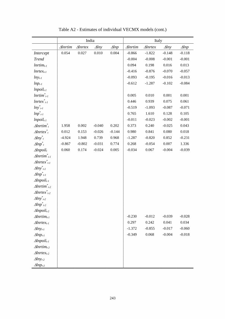
243
Table A2 - Estimates of individual VECMX models (cont.)
India Italy
lnrtim lnrtex lny lnp lnrtim lnrtex lny lnp
Intercept 0.054 0.027 0.010 0.004 -0.866 -1.822 -0.148 -0.118
Trend -0.004 -0.008 -0.001 -0.001
lnrtimt-1 0.094 0.198 0.016 0.013
lnrtext-1 -0.416 -0.876 -0.070 -0.057
lnyt-1 -0.093 -0.195 -0.016 -0.013
lnpt-1 -0.612 -1.287 -0.102 -0.084
lnpoilt-1
lnrtim*t-1 0.005 0.010 0.001 0.001
lnrtex*t-1 0.446 0.939 0.075 0.061
lny*t-1 -0.519 -1.093 -0.087 -0.071
lnp*t-1 0.765 1.610 0.128 0.105
lnpoilt-1 -0.011 -0.023 -0.002 -0.001
lnrtim*t 1.958 0.002 -0.040 0.202 0.373 0.240 -0.025 0.043
lnrtex*t 0.012 0.153 -0.026 -0.144 0.980 0.841 0.080 0.018
lny*t -4.924 1.948 0.739 0.968 -1.287 -0.820 0.852 -0.231
lnp*t -0.867 -0.802 -0.031 0.774 0.268 -0.054 0.007 1.336
lnpoilt 0.060 0.174 -0.024 0.005 -0.034 0.067 -0.004 -0.039
lnrtim*t-1
lnrtex*t-1
lny*t-1
lnp*t-1
lnpoilt-1
lnrtim*t-2
lnrtex*t-2
lny*t-2
lnp*t-2
lnpoilt-2
lnrtimt-1 -0.230 -0.012 -0.039 -0.028
lnrtext-1 0.297 0.242 0.041 0.034
lnyt-1 -1.372 -0.855 -0.017 -0.060
lnpt-1 -0.349 0.068 -0.004 -0.018
lnpoilt-1
lnrtimt-2
lnrtext-2
lnyt-2
lnpt-2

244
Table A2 - Estimates of individual VECMX models (cont.)
Japan Korea
lnrtim lnrtex lny lnp lnrtim lnrtex lnycons lnp
Intercept 5.313 4.395 -0.165 -0.630 1.085 1.686 0.109 0.260
Trend 0.039 0.032 -0.001 -0.005 0.006 0.009 0.001 0.001
lnrtimt-1 -0.715 -0.587 0.021 0.084 -0.079 -0.121 -0.008 -0.020
lnrtext-1 -0.056 -0.046 0.002 0.007 -0.252 -0.387 -0.025 -0.063
lnyt-1 5.732 4.707 -0.170 -0.673 -0.453 -0.696 -0.046 -0.114
lnpt-1 0.404 0.331 -0.012 -0.047 -0.448 -0.688 -0.045 -0.112
lnpoilt-1
lnrtim*t-1 0.329 0.506 0.033 0.083
lnrtex*t-1 -0.177 -0.271 -0.018 -0.044
lny*t-1 -5.555 -4.562 0.165 0.653 -0.158 -0.243 -0.016 -0.040
lnp*t-1 0.209 0.172 -0.006 -0.025 0.209 0.320 0.021 0.052
lnpoilt-1 -0.071 -0.058 0.002 0.008 0.056 0.086 0.006 0.014
lnrtim*t -0.009 1.840 -0.031 -0.284
lnrtex*t 0.391 -0.479 0.042 0.136
lny*t -0.224 -3.159 0.776 2.001 2.760 -4.733 0.886 1.521
lnp*t -1.304 -1.046 0.010 0.614 -1.260 0.733 -0.112 0.438
lnpoilt 0.277 0.173 0.006 -0.062 0.344 -0.637 0.044 0.262
lnrtim*t-1
lnrtex*t-1
lny*t-1
lnp*t-1
lnpoilt-1
lnrtim*t-2
lnrtex*t-2
lny*t-2
lnp*t-2
lnpoilt-2
lnrtimt-1 0.203 0.069 -0.006 0.098 0.186 -0.050 0.083 0.163
lnrtext-1 -0.224 -0.142 0.008 -0.075 0.094 -0.105 0.027 0.064
lnyt-1 0.739 1.490 0.083 0.063 -0.182 2.548 -0.203 -1.034
lnpt-1 -0.531 -0.326 0.000 0.045 -0.173 -0.493 0.066 0.147
lnpoilt-1
lnrtimt-2
lnrtext-2
lnyt-2
lnpt-2
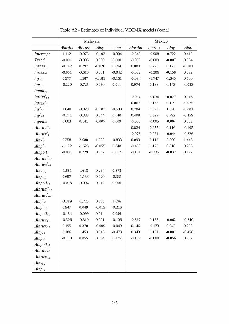
245
Table A2 - Estimates of individual VECMX models (cont.)
Malaysia Mexico
lnrtim lnrtex lny lnp lnrtim lnrtex lny lnp
Intercept 1.112 -0.073 -0.103 -0.304 -0.340 -0.908 -0.722 0.412
Trend -0.001 -0.005 0.000 0.000 -0.003 -0.009 -0.007 0.004
lnrtimt-1 -0.142 0.797 -0.026 0.094 0.089 0.225 0.173 -0.101
lnrtext-1 -0.001 -0.613 0.031 -0.042 -0.082 -0.206 -0.158 0.092
lnyt-1 0.977 1.587 -0.181 -0.161 -0.694 -1.747 -1.345 0.780
lnpt-1 -0.220 -0.725 0.060 0.011 0.074 0.186 0.143 -0.083
lnpoilt-1
lnrtim*t-1 -0.014 -0.036 -0.027 0.016
lnrtex*t-1 0.067 0.168 0.129 -0.075
lny*t-1 1.840 -0.020 -0.187 -0.508 0.784 1.973 1.520 -0.881
lnp*t-1 -0.241 -0.383 0.044 0.040 0.408 1.029 0.792 -0.459
lnpoilt-1 0.003 0.141 -0.007 0.009 -0.002 -0.005 -0.004 0.002
lnrtim*t 0.824 0.675 0.116 -0.105
lnrtex*t -0.073 0.261 -0.044 -0.226
lny*t 0.258 2.688 1.082 -0.833 0.099 0.113 2.360 1.443
lnp*t -1.122 -1.623 -0.055 0.848 -0.453 1.125 0.818 0.203
lnpoilt -0.001 0.229 0.032 0.017 -0.101 -0.235 -0.032 0.172
lnrtim*t-1
lnrtex*t-1
lny*t-1 -1.681 1.618 0.264 0.878
lnp*t-1 0.657 -1.138 0.020 -0.331
lnpoilt-1 -0.018 -0.094 0.012 0.006
lnrtim*t-2
lnrtex*t-2
lny*t-2 -3.389 -1.725 0.308 1.696
lnp*t-2 0.947 0.049 -0.015 -0.216
lnpoilt-2 -0.184 -0.099 0.014 0.096
lnrtimt-1 -0.306 -0.310 0.001 -0.106 -0.367 0.155 -0.062 -0.240
lnrtext-1 0.195 0.370 -0.009 -0.040 0.146 -0.173 0.042 0.252
lnyt-1 0.186 1.453 0.015 -0.478 0.343 1.191 -0.001 -0.458
lnpt-1 -0.110 0.855 0.034 0.175 -0.107 -0.600 -0.056 0.282
lnpoilt-1
lnrtimt-2
lnrtext-2
lnyt-2
lnpt-2

246
Table A2 - Estimates of individual VECMX models (cont.)
Netherlands New Zealand
lnrtim lnrtex lny lnp lnrtim lnrtex lny lnp
Intercept -2.428 3.935 -0.014 -0.461 0.005 0.006 -0.001 -0.005
Trend -0.003 0.004 0.000 -0.001
lnrtimt-1 -0.188 0.303 -0.001 -0.036
lnrtext-1 0.299 -0.483 0.002 0.057
lnyt-1 0.659 -1.066 0.004 0.125
lnpt-1 -0.430 0.695 -0.002 -0.081
lnpoilt-1
lnrtim*t-1 0.435 -0.704 0.002 0.082
lnrtex*t-1 -0.259 0.419 -0.001 -0.049
lny*t-1 -1.887 3.052 -0.011 -0.357
lnp*t-1 0.650 -1.051 0.004 0.123
lnpoilt-1 -0.036 0.059 0.000 -0.007
lnrtim*t 0.553 0.038 0.002 0.107 0.394 0.483 0.021 -0.271
lnrtex*t -0.252 0.506 0.017 -0.044 -0.152 -0.324 -0.001 0.379
lny*t 0.185 1.468 0.827 -0.595 1.518 0.394 0.796 0.637
lnp*t -0.056 -0.237 -0.020 1.349 -0.741 -0.083 -0.007 1.715
lnpoilt -0.045 0.039 -0.007 -0.047 0.094 0.014 -0.012 0.007
lnrtim*t-1
lnrtex*t-1
lny*t-1
lnp*t-1
lnpoilt-1
lnrtim*t-2
lnrtex*t-2
lny*t-2
lnp*t-2
lnpoilt-2
lnrtimt-1
lnrtext-1
lnyt-1
lnpt-1
lnpoilt-1
lnrtimt-2
lnrtext-2
lnyt-2
lnpt-2
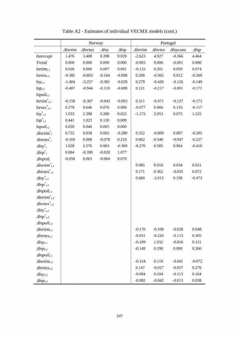
247
Table A2 - Estimates of individual VECMX models (cont.)
Norway Portugal
lnrtim lnrtex lny lnp lnrtim lnrtex lnycons lnp
Intercept 1.476 3.408 0.398 0.029 -2.623 4.927 -0.366 4.464
Trend 0.000 0.000 0.000 0.000 -0.003 0.006 -0.001 0.006
lnrtimt-1 0.026 0.060 0.007 0.001 -0.133 0.201 0.059 0.074
lnrtext-1 -0.385 -0.893 -0.104 -0.008 0.200 -0.365 0.012 -0.309
lnyt-1 -1.404 -3.257 -0.381 -0.029 0.279 -0.420 -0.126 -0.149
lnpt-1 -0.407 -0.944 -0.110 -0.008 0.121 -0.217 -0.001 -0.171
lnpoilt-1
lnrtim*t-1 -0.158 -0.367 -0.043 -0.003 0.311 -0.471 -0.137 -0.173
lnrtex*t-1 0.278 0.646 0.076 0.006 -0.077 0.066 0.116 -0.117
lny*t-1 1.033 2.398 0.280 0.022 -1.173 2.053 0.075 1.525
lnp*t-1 0.441 1.023 0.120 0.009
lnpoilt-1 0.020 0.046 0.005 0.000
lnrtim*t 0.732 0.038 0.065 -0.280 0.352 -0.009 0.007 -0.285
lnrtex*t -0.169 0.008 -0.078 0.210 0.662 0.548 -0.047 -0.227
lny*t 1.028 2.576 0.903 -0.369 -0.270 0.585 0.964 -0.416
lnp*t 0.084 -0.398 -0.020 1.077
lnpoilt -0.058 0.063 -0.004 0.070
lnrtim*t-1 0.085 0.016 0.034 0.021
lnrtex*t-1 0.171 0.362 -0.035 0.072
lny*t-1 0.660 -2.015 0.338 -0.473
lnp*t-1
lnpoilt-1
lnrtim*t-2
lnrtex*t-2
lny*t-2
lnp*t-2
lnpoilt-2
lnrtimt-1 -0.170 -0.108 -0.028 0.048
lnrtext-1 -0.031 -0.220 -0.113 0.305
lnyt-1 -0.109 1.032 -0.016 0.121
lnpt-1 -0.149 0.190 0.000 0.366
lnpoilt-1
lnrtimt-2 -0.154 0.110 -0.041 -0.072
lnrtext-2 0.147 -0.027 -0.057 0.276
lnyt-2 -0.094 0.104 -0.113 0.164
lnpt-2 -0.082 -0.042 -0.013 0.038

248
Table A2 - Estimates of individual VECMX models (cont.)
South Africa Spain
lnrtim lnrtex lny lnp lnrtim lnrtex lny lnp
Intercept 4.017 2.860 0.067 -0.574 0.565 -0.295 -0.198 -0.157
Trend 0.015 0.011 0.000 -0.002 0.000 0.000 0.000 0.000
lnrtimt-1 -0.676 -0.479 -0.011 0.095 -0.160 0.087 0.057 0.046
lnrtext-1 -0.148 -0.105 -0.002 0.021 0.088 -0.047 -0.031 -0.025
lnyt-1 -0.756 -0.536 -0.012 0.107 0.650 -0.352 -0.234 -0.185
lnpt-1 -0.407 -0.288 -0.007 0.057 -0.336 0.182 0.121 0.096
lnpoilt-1
lnrtim*t-1 -1.087 -0.770 -0.018 0.153 -0.124 0.067 0.045 0.035
lnrtex*t-1 1.198 0.849 0.020 -0.169 0.106 -0.057 -0.038 -0.030
lny*t-1 1.310 0.929 0.021 -0.185 -1.103 0.597 0.396 0.314
lnp*t-1 0.392 0.278 0.006 -0.055 0.408 -0.221 -0.147 -0.116
lnpoilt-1 0.098 0.069 0.002 -0.014 0.022 -0.012 -0.008 -0.006
lnrtim*t 0.154 -0.310 -0.083 0.436 0.351 -0.016 -0.032 0.098
lnrtex*t -0.325 0.864 0.037 -0.306 0.239 0.373 0.049 0.016
lny*t -0.498 -1.992 0.408 0.421 1.325 0.662 0.982 -0.394
lnp*t 0.503 0.174 -0.024 1.262 0.012 -0.022 -0.018 1.298
lnpoilt -0.013 -0.082 -0.004 0.132 0.017 -0.011 -0.004 -0.034
lnrtim*t-1 0.110 0.027 -0.036 -0.001
lnrtex*t-1 -0.049 0.276 0.054 0.019
lny*t-1 0.184 -0.859 -0.201 -0.649
lnp*t-1 -0.785 -0.647 0.066 0.862
lnpoilt-1 -0.011 0.034 -0.001 -0.003
lnrtim*t-2
lnrtex*t-2
lny*t-2
lnp*t-2
lnpoilt-2
lnrtimt-1 0.032 -0.176 -0.029 0.018
lnrtext-1 0.029 -0.213 0.046 -0.007
lnyt-1 0.514 1.144 0.052 0.312
lnpt-1 0.812 0.565 -0.058 -0.736
lnpoilt-1
lnrtimt-2
lnrtext-2
lnyt-2
lnpt-2

249
Table A2 - Estimates of individual VECMX models (cont.)
Sweden Thailand
lnrtim lnrtex lny lnp lnrtim lnrtex lny lnp
Intercept -0.003 0.021 0.001 -0.004 1.341 -0.451 -0.356 0.567
Trend 0.008 0.002 0.000 -0.001
lnrtimt-1 -0.359 0.055 0.070 -0.083
lnrtext-1 -0.350 -0.169 -0.014 0.153
lnyt-1 0.375 -0.630 -0.284 0.684
lnpt-1 0.329 0.493 0.136 -0.493
lnpoilt-1
lnrtim*t-1 0.353 -0.109 -0.089 0.138
lnrtex*t-1 0.072 0.261 0.086 -0.267
lny*t-1 -1.055 -0.231 0.061 0.169
lnp*t-1 -0.945 -0.640 -0.105 0.603
lnpoilt-1 0.097 0.007 -0.011 0.000
lnrtim*t 0.857 -0.304 0.097 -0.243 1.212 0.953 -0.005 -0.010
lnrtex*t 0.352 0.121 -0.101 0.213 -0.387 -0.070 0.002 0.001
lny*t 0.708 0.143 1.358 1.199 -2.485 1.663 0.551 1.266
lnp*t -0.106 -0.146 0.012 1.280 -0.312 0.482 0.259 1.461
lnpoilt 0.094 -0.137 0.013 0.058 -0.101 0.064 -0.018 0.031
lnrtim*t-1 0.440 0.058 -0.048 -0.418
lnrtex*t-1 -0.657 -0.184 -0.064 0.242
lny*t-1 0.112 0.999 -0.189 -0.762
lnp*t-1 -0.881 -0.153 -0.195 -0.450
lnpoilt-1 -0.052 0.013 0.030 -0.075
lnrtim*t-2
lnrtex*t-2
lny*t-2
lnp*t-2
lnpoilt-2
lnrtimt-1 -0.317 -0.003 -0.016 0.150
lnrtext-1 0.497 -0.184 0.042 -0.001
lnyt-1 1.198 0.210 0.320 -0.599
lnpt-1 0.561 -0.259 0.081 0.459
lnpoilt-1
lnrtimt-2 -0.007 0.044 -0.002 0.039
lnrtext-2 0.366 -0.080 -0.019 0.029
lnyt-2 0.818 0.788 0.191 -0.202
lnpt-2 0.373 -0.430 -0.064 0.037

250
Table A2 - Estimates of individual VECMX models (cont.)
United Kingdom USA
lnrtim lnrtex lny lnp lnrtim lnrtex lny lnp lnpoil
Intercept 5.662 7.177 -0.270 1.172 -0.084 0.009 0.004 -0.018 -0.310
Trend 0.004 0.006 0.000 0.001 0.004 -0.001 0.000 0.001 0.017
lnrtimt-1 -0.899 -1.141 0.043 -0.186 -0.346 0.072 0.025 -0.106 -1.429
lnrtext-1 0.058 0.073 -0.003 0.012 0.331 -0.069 -0.024 0.101 1.364
lnyt-1 2.359 2.992 -0.113 0.488 0.477 -0.099 -0.035 0.145 1.968
lnpt-1 -0.055 -0.070 0.003 -0.011 -0.756 0.158 0.055 -0.230 -3.118
lnpoilt-1 0.001 0.000 0.000 0.000 0.004
lnrtim*t-1 -0.018 -0.023 0.001 -0.004 -0.142 0.030 0.010 -0.043 -0.586
lnrtex*t-1 0.270 0.343 -0.013 0.056 0.115 -0.024 -0.008 0.035 0.474
lny*t-1 -0.919 -1.166 0.044 -0.190
lnp*t-1 -0.164 -0.208 0.008 -0.034 0.059 -0.012 -0.004 0.018 0.242
lnpoilt-1 0.032 0.040 -0.002 0.007
lnrtim*t 0.146 0.491 0.027 -0.476 0.551 0.869 0.025 -0.014 0.966
lnrtex*t 0.496 0.042 0.028 0.224 0.251 0.077 0.013 0.009 -0.110
lny*t -0.050 1.025 0.637 0.987
lnp*t -0.001 0.346 0.020 0.553 0.216 0.319 -0.046 0.140 3.676
lnpoilt -0.030 0.009 -0.024 0.074
lnrtim*t-1 -0.025 0.890 -0.072 -0.137
lnrtex*t-1 0.059 0.013 0.053 0.161
lny*t-1 1.476 4.215 -0.295 -0.528
lnp*t-1 0.450 0.365 -0.036 -0.016
lnpoilt-1 0.075 -0.098 0.025 0.000
lnrtim*t-2 0.063 0.152 -0.047 -0.379
lnrtex*t-2 0.251 -0.092 0.083 0.117
lny*t-2 1.276 1.628 -0.085 0.948
lnp*t-2 0.376 1.150 -0.012 -0.020
lnpoilt-2 -0.042 0.033 -0.016 -0.024
lnrtimt-1 0.080 0.417 -0.008 0.036 -0.182 0.126 0.054 0.006 -0.563
lnrtext-1 -0.128 -0.736 0.008 0.093 -0.118 -0.387 -0.086 0.000 0.259
lnyt-1 -0.484 -3.822 0.654 0.610 0.242 1.375 0.490 -0.244 -1.904
lnpt-1 -0.642 -0.174 -0.003 0.298 1.012 0.454 0.272 0.076 -0.760
lnpoilt-1 0.006 0.058 0.004 -0.005 0.061
lnrtimt-2 -0.111 0.000 -0.026 0.236
lnrtext-2 -0.086 -0.149 -0.003 0.086
lnyt-2 -2.281 -2.629 0.023 -0.919
lnpt-2 -0.156 -0.995 0.032 -0.250

251
Figure A1 - Generalised impulse responses of a negative shock to China’s real income on real income across countries/regions
-0.14
-0.12
-0.1
-0.08
-0.06
-0.04
-0.02
0
0.02
0.04
0.06
0 4 8 12 16 20 24 28 32 36 40
Number of quarters
China - Real Income (lny)
-0.06
-0.04
-0.02
0
0.02
0.04
0.06
0 4 8 12 16 20 24 28 32 36 40
Number of quarters
Asia - Real Income (lny)
-0.08
-0.06
-0.04
-0.02
0
0.02
0.04
0.06
0.08
0 4 8 12 16 20 24 28 32 36 40
Number of quarters
South Africa - Real Income (lny)
-0.04
-0.03
-0.02
-0.01
0
0.01
0.02
0.03
0.04
0.05
0 4 8 12 16 20 24 28 32 36 40
Number of quarters
Oceania - Real Income (lny)

252
Figure A1 - Generalised impulse responses of a negative shock to China’s real income on real income across countries/regions (cont.)
-0.06
-0.04
-0.02
0
0.02
0.04
0.06
0 4 8 12 16 20 24 28 32 36 40
Number of quarters
Europe - Real Income (lny)
-0.2
-0.15
-0.1
-0.05
0
0.05
0.1
0.15
0.2
0 4 8 12 16 20 24 28 32 36 40
Number of quarters
South America - Real Income (lny)
-0.04
-0.03
-0.02
-0.01
0
0.01
0.02
0.03
0.04
0 4 8 12 16 20 24 28 32 36 40
Number of quarters
Canada - Real Income (lny)
-0.4
-0.3
-0.2
-0.1
0
0.1
0.2
0.3
0 4 8 12 16 20 24 28 32 36 40
Number of quarters
Mexico - Real Income (lny)

253
Figure A1 - Generalised impulse responses of a negative shock to China’s real income on real income across countries/regions (cont.)
Notes: ‘Asia’ include India, Japan, Korea, Malaysia, and Thailand, but China is displayed individually;
‘Europe’ include Austria, France, Germany, Italy, Netherlands, Norway, Portugal, Spain, Sweden, and UK;
‘Oceania’ include Australia and New Zealand;
‘South America’ include Argentina and Brazil;
To highlight the importance of USA’s economy, countries of the North America are not aggregated;
The lines are bootstrap mean estimates with 90% bootstrap error bounds.
-0.015
-0.01
-0.005
0
0.005
0.01
0.015
0 4 8 12 16 20 24 28 32 36 40
Number of quarters
USA - Real Income (lny)

254
Figure A2 - Generalised impulse responses of a negative shock to China’s real income on own price across countries/regions
-0.2
-0.15
-0.1
-0.05
0
0.05
0.1
0.15
0 4 8 12 16 20 24 28 32 36 40
Number of quarters
China - Own Price (lnp)
-0.4
-0.3
-0.2
-0.1
0
0.1
0.2
0.3
0 4 8 12 16 20 24 28 32 36 40
Number of quarters
Asia - Own Price (lnp)
-1
-0.8
-0.6
-0.4
-0.2
0
0.2
0.4
0.6
0.8
1
0 4 8 12 16 20 24 28 32 36 40
Number of quarters
South Africa - Own Price (lnp)
-0.4
-0.3
-0.2
-0.1
0
0.1
0.2
0.3
0.4
0 4 8 12 16 20 24 28 32 36 40
Number of quarters
Oceania - Own Price (lnp)
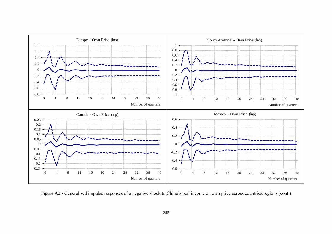
255
Figure A2 - Generalised impulse responses of a negative shock to China’s real income on own price across countries/regions (cont.)
-0.8
-0.6
-0.4
-0.2
0
0.2
0.4
0.6
0.8
0 4 8 12 16 20 24 28 32 36 40
Number of quarters
Europe - Own Price (lnp)
-1
-0.8
-0.6
-0.4
-0.2
0
0.2
0.4
0.6
0.8
1
0 4 8 12 16 20 24 28 32 36 40
Number of quarters
South America - Own Price (lnp)
-0.25
-0.2
-0.15
-0.1
-0.05
0
0.05
0.1
0.15
0.2
0.25
0 4 8 12 16 20 24 28 32 36 40
Number of quarters
Canada - Own Price (lnp)
-0.6
-0.4
-0.2
0
0.2
0.4
0.6
0 4 8 12 16 20 24 28 32 36 40
Number of quarters
Mexico - Own Price (lnp)

256
Figure A2 - Generalised impulse responses of a negative shock to China’s real income on own price across countries/regions (cont.)
Notes: ‘Asia’ include India, Japan, Korea, Malaysia, and Thailand, but China is displayed individually;
‘Europe’ include Austria, France, Germany, Italy, Netherlands, Norway, Portugal, Spain, Sweden, and UK;
‘Oceania’ include Australia and New Zealand;
‘South America’ include Argentina and Brazil;
To highlight the importance of USA’s economy, countries of the North America are not aggregated;
The lines are bootstrap mean estimates with 90% bootstrap error bounds.
-0.1
-0.08
-0.06
-0.04
-0.02
0
0.02
0.04
0.06
0.08
0 4 8 12 16 20 24 28 32 36 40
Number of quarters
USA - Own Price (lnp)

257
Figure A3 - Generalised impulse responses of a negative shock to China’s real income on real tourism imports across countries/regions
-2
-1.5
-1
-0.5
0
0.5
1
1.5
2
0 4 8 12 16 20 24 28 32 36 40
Number of quarters
China - Real Tourism Imports (lnrtim)
-0.8
-0.6
-0.4
-0.2
0
0.2
0.4
0.6
0 4 8 12 16 20 24 28 32 36 40
Number of quarters
South Africa - Real Tourism Imports (lnrtim)
-2
-1.5
-1
-0.5
0
0.5
1
1.5
0 4 8 12 16 20 24 28 32 36 40
Number of quarters
Asia - Real Tourism Imports (lnrtim)
-0.8
-0.6
-0.4
-0.2
0
0.2
0.4
0.6
0 4 8 12 16 20 24 28 32 36 40
Number of quarters
Oceania - Real Tourism Imports (lnrtim)

258
Figure A3 - Generalised impulse responses of a negative shock to China’s real income on real tourism imports across countries/regions (cont.)
-0.1
-0.08
-0.06
-0.04
-0.02
0
0.02
0.04
0.06
0.08
0.1
0 4 8 12 16 20 24 28 32 36 40
Number of quarters
Canada - Real Tourism Imports (lnrtim)
-0.2
-0.15
-0.1
-0.05
0
0.05
0.1
0.15
0.2
0 4 8 12 16 20 24 28 32 36 40
Number of quarters
Mexico - Real Tourism Imports (lnrtim)
-0.2
-0.15
-0.1
-0.05
0
0.05
0.1
0.15
0.2
0 4 8 12 16 20 24 28 32 36 40
Number of quarters
Europe - Real Tourism Imports (lnrtim)
-1.5
-1
-0.5
0
0.5
1
1.5
0 4 8 12 16 20 24 28 32 36 40
Number of quarters
South America - Real Tourism Imports (lnrtim)

259
Figure A3 - Generalised impulse responses of a negative shock to China’s real income on real tourism imports across countries/regions (cont.)
Notes: ‘Asia’ include India, Japan, Korea, Malaysia, and Thailand, but China is displayed individually;
‘Europe’ include Austria, France, Germany, Italy, Netherlands, Norway, Portugal, Spain, Sweden, and UK;
‘Oceania’ include Australia and New Zealand;
‘South America’ include Argentina and Brazil;
To highlight the importance of USA’s economy, countries of the North America are not aggregated;
The lines are bootstrap mean estimates with 90% bootstrap error bounds.
-0.8
-0.6
-0.4
-0.2
0
0.2
0.4
0.6
0 4 8 12 16 20 24 28 32 36 40
Number of quarters
USA - Real Tourism Imports (lnrtim)
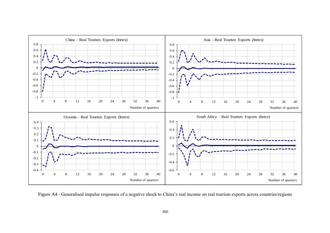
260
Figure A4 - Generalised impulse responses of a negative shock to China’s real income on real tourism exports across countries/regions
-1
-0.8
-0.6
-0.4
-0.2
0
0.2
0.4
0.6
0.8
0 4 8 12 16 20 24 28 32 36 40
Number of quarters
China - Real Tourism Exports (lnrtex)
-0.6
-0.4
-0.2
0
0.2
0.4
0.6
0 4 8 12 16 20 24 28 32 36 40
Number of quarters
South Africa - Real Tourism Exports (lnrtex)
-1
-0.8
-0.6
-0.4
-0.2
0
0.2
0.4
0.6
0.8
0 4 8 12 16 20 24 28 32 36 40
Number of quarters
Asia - Real Tourism Exports (lnrtex)
-0.4
-0.3
-0.2
-0.1
0
0.1
0.2
0.3
0.4
0 4 8 12 16 20 24 28 32 36 40
Number of quarters
Oceania - Real Tourism Exports (lnrtex)

261
Figure A4 - Generalised impulse responses of a negative shock to China’s real income on real tourism exports across countries/regions (cont.)
-0.15
-0.1
-0.05
0
0.05
0.1
0 4 8 12 16 20 24 28 32 36 40
Number of quarters
Canada - Real Tourism Exports (lnrtex)
-0.6
-0.4
-0.2
0
0.2
0.4
0.6
0 4 8 12 16 20 24 28 32 36 40
Number of quarters
Mexico - Real Tourism Exports (lnrtex)
-0.3
-0.2
-0.1
0
0.1
0.2
0.3
0 4 8 12 16 20 24 28 32 36 40
Number of quarters
Europe - Real Tourism Exports (lnrtex)
-1.5
-1
-0.5
0
0.5
1
1.5
0 4 8 12 16 20 24 28 32 36 40
Number of quarters
South America - Real Tourism Exports (lnrtex)

262
Figure A4 - Generalised impulse responses of a negative shock to China’s real income on real tourism exports across countries/regions (cont.)
Notes: ‘Asia’ include India, Japan, Korea, Malaysia, and Thailand, but China is displayed individually;
‘Europe’ include Austria, France, Germany, Italy, Netherlands, Norway, Portugal, Spain, Sweden, and UK;
‘Oceania’ include Australia and New Zealand;
‘South America’ include Argentina and Brazil;
To highlight the importance of USA’s economy, countries of the North America are not aggregated;
The lines are bootstrap mean estimates with 90% bootstrap error bounds.
-0.8
-0.6
-0.4
-0.2
0
0.2
0.4
0.6
0 4 8 12 16 20 24 28 32 36 40
Number of quarters
USA - Real Tourism Exports (lnrtex)

263
Figure A5 - Generalised impulse responses of a negative shock to China’s own price on real income across countries/regions
-0.12
-0.1
-0.08
-0.06
-0.04
-0.02
0
0.02
0.04
0.06
0 4 8 12 16 20 24 28 32 36 40
Number of quarters
China - Real Income (lny)
-0.05
-0.04
-0.03
-0.02
-0.01
0
0.01
0.02
0.03
0.04
0.05
0 4 8 12 16 20 24 28 32 36 40
Number of quarters
Asia - Real Income (lny)
-0.06
-0.04
-0.02
0
0.02
0.04
0.06
0.08
0 4 8 12 16 20 24 28 32 36 40
Number of quarters
South Africa - Real Income (lny)
-0.03
-0.02
-0.01
0
0.01
0.02
0.03
0.04
0 4 8 12 16 20 24 28 32 36 40
Number of quarters
Oceania - Real Income (lny)
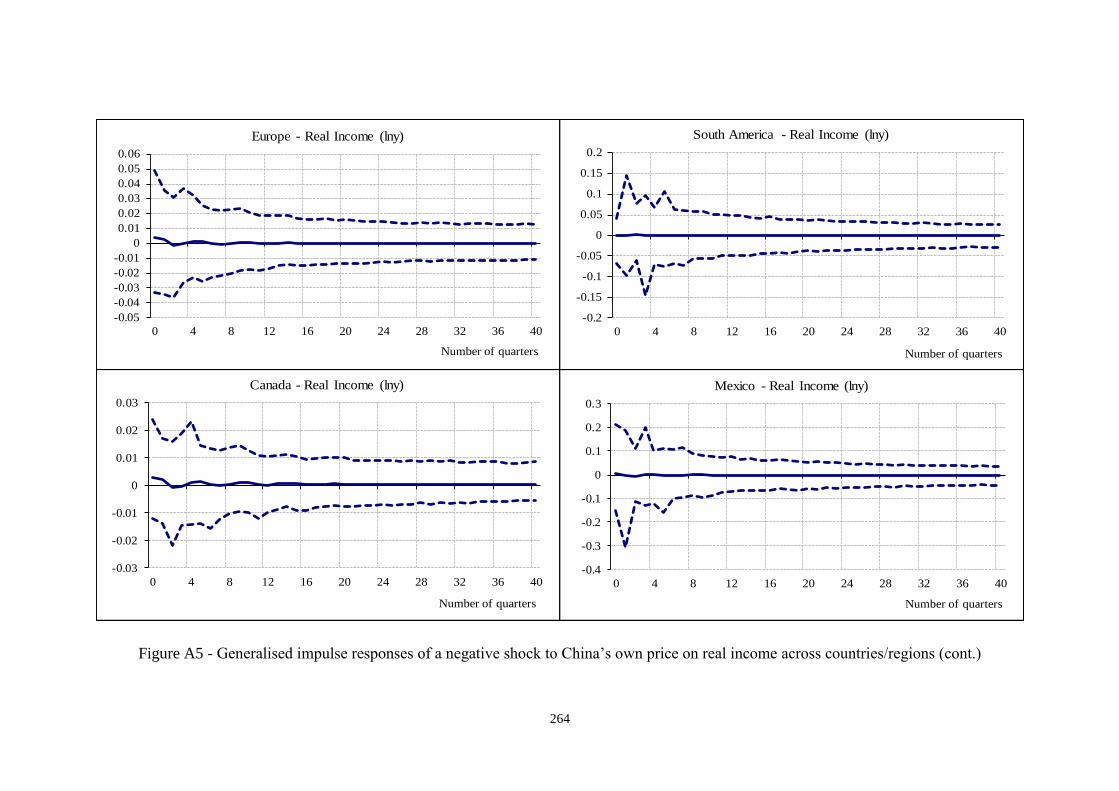
264
Figure A5 - Generalised impulse responses of a negative shock to China’s own price on real income across countries/regions (cont.)
-0.05
-0.04
-0.03
-0.02
-0.01
0
0.01
0.02
0.03
0.04
0.05
0.06
0 4 8 12 16 20 24 28 32 36 40
Number of quarters
Europe - Real Income (lny)
-0.2
-0.15
-0.1
-0.05
0
0.05
0.1
0.15
0.2
0 4 8 12 16 20 24 28 32 36 40
Number of quarters
South America - Real Income (lny)
-0.03
-0.02
-0.01
0
0.01
0.02
0.03
0 4 8 12 16 20 24 28 32 36 40
Number of quarters
Canada - Real Income (lny)
-0.4
-0.3
-0.2
-0.1
0
0.1
0.2
0.3
0 4 8 12 16 20 24 28 32 36 40
Number of quarters
Mexico - Real Income (lny)

265
Figure A5 - Generalised impulse responses of a negative shock to China’s own price on real income across countries/regions (cont.)
Notes: ‘Asia’ include India, Japan, Korea, Malaysia, and Thailand, but China is displayed individually;
‘Europe’ include Austria, France, Germany, Italy, Netherlands, Norway, Portugal, Spain, Sweden, and UK;
‘Oceania’ include Australia and New Zealand;
‘South America’ include Argentina and Brazil;
To highlight the importance of USA’s economy, countries of the North America are not aggregated;
The lines are bootstrap mean estimates with 90% bootstrap error bounds.
-0.015
-0.01
-0.005
0
0.005
0.01
0.015
0.02
0 4 8 12 16 20 24 28 32 36 40
Number of quarters
USA - Real Income (lny)
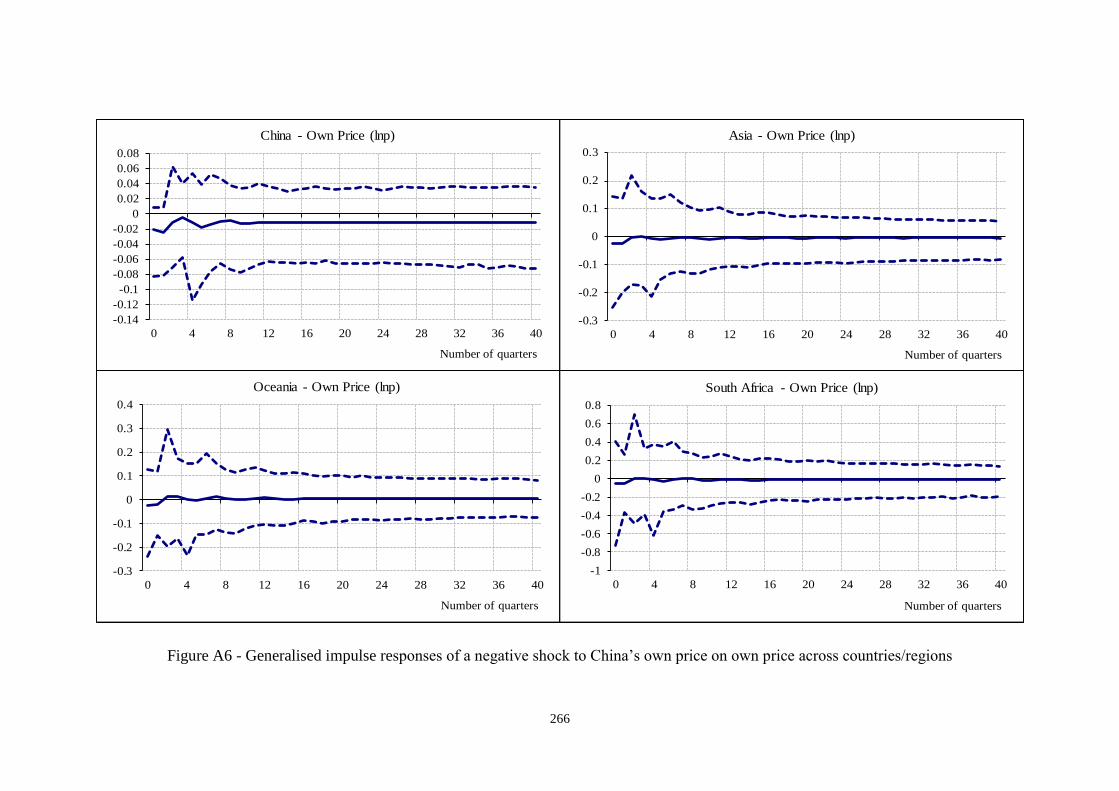
266
Figure A6 - Generalised impulse responses of a negative shock to China’s own price on own price across countries/regions
-0.14
-0.12
-0.1
-0.08
-0.06
-0.04
-0.02
0
0.02
0.04
0.06
0.08
0 4 8 12 16 20 24 28 32 36 40
Number of quarters
China - Own Price (lnp)
-0.3
-0.2
-0.1
0
0.1
0.2
0.3
0 4 8 12 16 20 24 28 32 36 40
Number of quarters
Asia - Own Price (lnp)
-1
-0.8
-0.6
-0.4
-0.2
0
0.2
0.4
0.6
0.8
0 4 8 12 16 20 24 28 32 36 40
Number of quarters
South Africa - Own Price (lnp)
-0.3
-0.2
-0.1
0
0.1
0.2
0.3
0.4
0 4 8 12 16 20 24 28 32 36 40
Number of quarters
Oceania - Own Price (lnp)
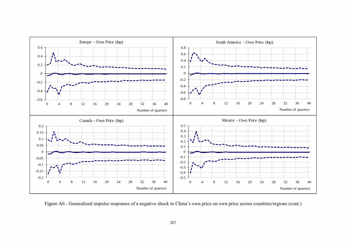
267
Figure A6 - Generalised impulse responses of a negative shock to China’s own price on own price across countries/regions (cont.)
-0.6
-0.4
-0.2
0
0.2
0.4
0.6
0 4 8 12 16 20 24 28 32 36 40
Number of quarters
Europe - Own Price (lnp)
-0.8
-0.6
-0.4
-0.2
0
0.2
0.4
0.6
0.8
0 4 8 12 16 20 24 28 32 36 40
Number of quarters
South America - Own Price (lnp)
-0.2
-0.15
-0.1
-0.05
0
0.05
0.1
0.15
0.2
0 4 8 12 16 20 24 28 32 36 40
Number of quarters
Canada - Own Price (lnp)
-0.5
-0.4
-0.3
-0.2
-0.1
0
0.1
0.2
0.3
0.4
0.5
0 4 8 12 16 20 24 28 32 36 40
Number of quarters
Mexico - Own Price (lnp)

268
Figure A6 - Generalised impulse responses of a negative shock to China’s own price on own price across countries/regions (cont.)
Notes: ‘Asia’ include India, Japan, Korea, Malaysia, and Thailand, but China is displayed individually;
‘Europe’ include Austria, France, Germany, Italy, Netherlands, Norway, Portugal, Spain, Sweden, and UK;
‘Oceania’ include Australia and New Zealand;
‘South America’ include Argentina and Brazil;
To highlight the importance of USA’s economy, countries of the North America are not aggregated;
The lines are bootstrap mean estimates with 90% bootstrap error bounds.
-0.08
-0.06
-0.04
-0.02
0
0.02
0.04
0.06
0 4 8 12 16 20 24 28 32 36 40
Number of quarters
USA - Own Price (lnp)

269
Figure A7 - Generalised impulse responses of a negative shock to China’s own price on real tourism imports across countries/regions
-1.5
-1
-0.5
0
0.5
1
1.5
0 4 8 12 16 20 24 28 32 36 40
Number of quarters
China - Real Tourism Imports (lnrtim)
-1.5
-1
-0.5
0
0.5
1
0 4 8 12 16 20 24 28 32 36 40
Number of quarters
Asia - Real Tourism Imports (lnrtim)
-0.8
-0.6
-0.4
-0.2
0
0.2
0.4
0.6
0 4 8 12 16 20 24 28 32 36 40
Number of quarters
South Africa - Real Tourism Imports (lnrtim)
-0.6
-0.4
-0.2
0
0.2
0.4
0.6
0 4 8 12 16 20 24 28 32 36 40
Number of quarters
Oceania - Real Tourism Imports (lnrtim)

270
Figure A7 - Generalised impulse responses of a negative shock to China’s own price on real tourism imports across countries/regions (cont.)
-0.2
-0.15
-0.1
-0.05
0
0.05
0.1
0.15
0.2
0 4 8 12 16 20 24 28 32 36 40
Number of quarters
Europe - Real Tourism Imports (lnrtim)
-1
-0.8
-0.6
-0.4
-0.2
0
0.2
0.4
0.6
0.8
1
1.2
0 4 8 12 16 20 24 28 32 36 40
Number of quarters
South America - Real Tourism Imports (lnrtim)
-0.08
-0.06
-0.04
-0.02
0
0.02
0.04
0.06
0.08
0 4 8 12 16 20 24 28 32 36 40
Number of quarters
Canada - Real Tourism Imports (lnrtim)
-0.15
-0.1
-0.05
0
0.05
0.1
0.15
0.2
0 4 8 12 16 20 24 28 32 36 40
Number of quarters
Mexico - Real Tourism Imports (lnrtim)
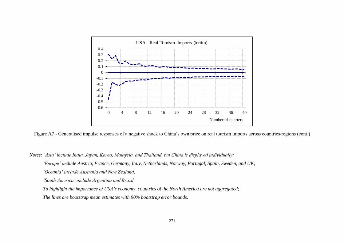
271
Figure A7 - Generalised impulse responses of a negative shock to China’s own price on real tourism imports across countries/regions (cont.)
Notes: ‘Asia’ include India, Japan, Korea, Malaysia, and Thailand, but China is displayed individually;
‘Europe’ include Austria, France, Germany, Italy, Netherlands, Norway, Portugal, Spain, Sweden, and UK;
‘Oceania’ include Australia and New Zealand;
‘South America’ include Argentina and Brazil;
To highlight the importance of USA’s economy, countries of the North America are not aggregated;
The lines are bootstrap mean estimates with 90% bootstrap error bounds.
-0.6
-0.5
-0.4
-0.3
-0.2
-0.1
0
0.1
0.2
0.3
0.4
0 4 8 12 16 20 24 28 32 36 40
Number of quarters
USA - Real Tourism Imports (lnrtim)

272
Figure A8 - Generalised impulse responses of a negative shock to China’s own price on real tourism exports across countries/regions
-0.8
-0.6
-0.4
-0.2
0
0.2
0.4
0.6
0.8
0 4 8 12 16 20 24 28 32 36 40
Number of quarters
China - Real Tourism Exports (lnrtex)
-0.8
-0.6
-0.4
-0.2
0
0.2
0.4
0.6
0 4 8 12 16 20 24 28 32 36 40
Number of quarters
Asia - Real Tourism Exports (lnrtex)
-0.5
-0.4
-0.3
-0.2
-0.1
0
0.1
0.2
0.3
0.4
0.5
0 4 8 12 16 20 24 28 32 36 40
Number of quarters
South Africa - Real Tourism Exports (lnrtex)
-0.4
-0.3
-0.2
-0.1
0
0.1
0.2
0.3
0 4 8 12 16 20 24 28 32 36 40
Number of quarters
Oceania - Real Tourism Exports (lnrtex)

273
Figure A8 - Generalised impulse responses of a negative shock to China’s own price on real tourism exports across countries/regions (cont.)
-0.25
-0.2
-0.15
-0.1
-0.05
0
0.05
0.1
0.15
0.2
0.25
0.3
0 4 8 12 16 20 24 28 32 36 40
Number of quarters
Europe - Real Tourism Exports (lnrtex)
-1.5
-1
-0.5
0
0.5
1
1.5
0 4 8 12 16 20 24 28 32 36 40
Number of quarters
South America - Real Tourism Exports (lnrtex)
-0.1
-0.08
-0.06
-0.04
-0.02
0
0.02
0.04
0.06
0.08
0.1
0 4 8 12 16 20 24 28 32 36 40
Number of quarters
Canada - Real Tourism Exports (lnrtex)
-0.5
-0.4
-0.3
-0.2
-0.1
0
0.1
0.2
0.3
0.4
0 4 8 12 16 20 24 28 32 36 40
Number of quarters
Mexico - Real Tourism Exports (lnrtex)

274
Figure A8 - Generalised impulse responses of a negative shock to China’s own price on real tourism exports across countries/regions (cont.)
Notes: ‘Asia’ include India, Japan, Korea, Malaysia, and Thailand, but China is displayed individually;
‘Europe’ include Austria, France, Germany, Italy, Netherlands, Norway, Portugal, Spain, Sweden, and UK;
‘Oceania’ include Australia and New Zealand;
‘South America’ include Argentina and Brazil;
To highlight the importance of USA’s economy, countries of the North America are not aggregated;
The lines are bootstrap mean estimates with 90% bootstrap error bounds.
-0.6
-0.5
-0.4
-0.3
-0.2
-0.1
0
0.1
0.2
0.3
0.4
0.5
0 4 8 12 16 20 24 28 32 36 40
Number of quarters
USA - Real Tourism Exports (lnrtex)

275
Bibliography
Abel, A. B., Bernanke, B., & Croushore, D. D. (2008). Macroeconomics (6th ed.).
Boston ; London: Pearson/Addison Wesley.
Abildgren, K. (2012). Business cycles, monetary transmission and shocks to
financial stability: empirical evidence from a new set of Danish quarterly national
accounts 1948-2010. Working Paper Series 1458, European Central Bank.
Retrieved January 9, 2015 from WWW:
http://www.ecb.europa.eu/pub/pdf/scpwps/ecbwp1458.pdf
Akal, M. (2004). Forecasting Turkey's tourism revenues by ARMAX model.
Tourism Management, 25(5), 565-580.
Akinboade, O. A., & Braimoh, L. A. (2010). International tourism and economic
development in South Africa: A Granger causality test. International Journal of
Tourism Research, 12(2), 149-163.
Albaladejo-Pina, I. P., & Díaz-Delfa, M. T. (2009). Tourist preferences for rural
house stays: Evidence from discrete choice modelling in Spain. Tourism
Management, 30(6), 805-811.
Albalate, D., & Bel, G. (2010). Tourism and urban public transport: Holding demand
pressure under supply constraints. Tourism Management, 31(3), 425-433. doi:
10.1016/j.tourman.2009.04.011
Alegre, J., Mateo, S., & Pou, L. (2011). A latent class approach to tourists’ length of
stay. Tourism Management, 32(3), 555-563.
Alvarez-Diaz, M., & Rossello-Nadal, J. (2010). Forecasting British tourist arrivals in
the Balearic Islands using meteorological variables. Tourism Economics, 16(1),
153-168.
Andersson, D. E. (2000). Hypothesis testing in hedonic price estimation: On the
selection of independent variables. Annals of Regional Science, 34, 293-304.
Araña, J. E., & León, C. J. (2008). The impact of terrorism on tourism
demand.Annals of Tourism Research, 35(2), 299-315.
276
Arellano, M., & Bond, S. (1991). Some tests of specification for panel data: Monte
Carlo evidence and an application to employment equations. The review of
economic studies, 58(2), 277-297.
Arellano, M., & Bover, O. (1995). Another look at the instrumental variable
estimation of error-components models. Journal of econometrics, 68(1), 29-51.
Artis, M. J., Fidrmuc, J., & Scharler, J. (2008). The transmission of business cycles
Implications for EMU enlargement1. Economics of Transition, 16(3), 559-582.
Artus, J. R. (1972). An Econometric Analysis of International Travel (Analyse
économétrique des voyages internationaux)(Análisis econométrico de los viajes
internacionales). Staff Papers-International Monetary Fund, 579-614.
Assaf, A. G., Barros, C. P., & Gil-Alana, L. A. (2011). Persistence in the Short-and
Long-Term Tourist Arrivals to Australia. Journal of Travel Research, 50(2), 213-
229.
Assenmacher, K. (2013). Forecasting the Swiss economy with a small GVAR
model. In F. di Mauro & M. H. Pesaran (Eds.), The GVAR Handbook: Structure
and Applications of a Macro Model of the Global Economy for Policy Analysis
(pp.244-254). Oxford: Oxford University Press.
Athanasopoulos, G., & de Silva, A. (2012). Multivariate exponential smoothing for
forecasting tourist arrivals. Journal of Travel Research, 51(5), 640-652.
Athanasopoulos, G., & Hyndman, R. J. (2008). Modelling and forecasting Australian
domestic tourism. Tourism Management, 29(1), 19-31.
Au, N., & Law, R. (2000). The application of rough sets to sightseeing
expenditures. Journal of Travel Research, 39(1), 70-77.
Au, N., & Law, R. (2002). Categorical classification of tourism dining. Annals of
Tourism Research, 29(3), 819-833.
Azarya, V. (2004). Globalization and international tourism in developing countries:
Marginality as a commercial commodity. Current Sociology, 52(6), 949-967.
277
Backhouse, R. (2010). The puzzle of modern economics: science or ideology.
Cambridge: Cambridge University Press.
Bagliano, F. C., & Morana, C. (2010). Business cycle comovement in the G-7:
common shocks or common transmission mechanisms?. Applied economics,
42(18), 2327-2345.
Bai, J., & Ng, S. (2004). A PANIC attack on unit roots and cointegration.
Econometrica, 72(4), 1127-1177.
Balaguer, J., & Cantavella-Jorda, M. (2002). Tourism as a long-run economic growth
factor: the Spanish case. Applied economics, 34(7), 877-884.
Balli, F., Balli, H. O., & Cebeci, K. (2013). Impacts of exported Turkish soap operas
and visa-free entry on inbound tourism to Turkey. Tourism Management, 37, 186-
192.
Barros, C. P., Butler, R., & Correia, A. (2010). The length of stay of golf tourism: A
survival analysis. Tourism Management, 31(1), 13-21.
Barros, C. P., & Machado, L. P. (2010). The length of stay in tourism. Annals of
Tourism Research, 37(3), 692-706.
Bartolomé, A., McAleer, M., Ramos, V., & Rey-Maquieira, J. (2009). Modelling air
passenger arrivals in the Balearic and Canary Islands, Spain. Tourism
Economics, 15(3), 481-500.
Belenkiy, M., & Riker, D. (2013). Modeling the International Tourism Expenditures
of Individual Travelers. Journal of Travel Research, 52(2), 202-211.
Belloumi, M. (2010). The relationship between tourism receipts, real effective
exchange rate and economic growth in Tunisia. International Journal of Tourism
Research, 12(5), 550-560.
Bilgic, A., Florkowski, W. J., Yoder, J., & Schreiner, D. F. (2008). Estimating
fishing and hunting leisure spending shares in the United States. Tourism
management, 29(4), 771-782.

278
Blundell, R., & Stoker, T. M. (2005). Heterogeneity and aggregation. Journal of
Economic Literature, 43(2), 347-391.
Bollerslev, T. (1986). Generalized autoregressive conditional heteroskedasticity.
Journal of econometrics, 31(3), 307-327.
Boschi, M. (2012). Long-and short-run determinants of capital flows to Latin
America: a long-run structural GVAR model. Empirical Economics, 43(3), 1041-
1071.
Breitung, J., & Pesaran, M. H. (2005). Unit roots and cointegration in panels (No.
2005, 42). Discussion paper Series 1/Volkswirtschaftliches Forschungszentrum
der Deutschen Bundesbank. Retrieved 4 March 2014, from WWW:
http://www.econstor.eu/bitstream/10419/19627/1/200542dkp.pdf
Brennan, M.J., and Schwartz, E.S. (1980). Analyzing Convertible Bonds. Journal of
Financial and Quantitative Analysis, 15, 907–929.
Bryant, R. C. (2003). Turbulent waters: cross-border finance and international
governance. Washington, DC: Brookings Institution Press.
Bussière, M., Chudik, A., & Sestieri, G. (2009). Modelling global trade flows:
results from a GVAR model. Working Paper Series 1087, European Central Bank.
Retrieved August 4, 2013 from:
http://www.ecb.europa.eu/pub/pdf/scpwps/ecbwp1087.pdf.
Candela, G., & Figini, P. (2012). The economics of tourism destinations (pp. 73-
130). Springer Berlin Heidelberg.
Cang, S. (2011). A non-linear tourism demand forecast combination model. Tourism
Economics, 17(1), 5-20.
Canova, F., & Ciccarelli, M. (2012). ClubMed? Cyclical fluctuations in the
Mediterranean basin. Journal of International Economics, 88(1), 162-175.
Cazanova, J., Ward, R. W., & Holland, S. (2013). Habit Persistence in Air Passenger
Traffic Destined for Florida. Journal of Travel Research.

279
Chan, K.C., Karolyi, G.A., Longstaff, F.A., & Sanders, A.B. (1992). An empirical
comparison of alternative models of the short-term interest rate. Journal of
Finance, 47, 1209–1227.
Chan, F., Lim, C., & McAleer, M. (2005). Modelling multivariate international
tourism demand and volatility. Tourism Management, 26(3), 459-471.
Chan, C. K., Witt, S. F., Lee, Y. C. E., & Song, H. (2010). Tourism forecast
combination using the CUSUM technique. Tourism Management, 31(6), 891-897.
Chang, Y. (2002). Nonlinear IV unit root tests in panels with cross-sectional
dependency. Journal of Econometrics, 110(2), 261-292.
Chang, C. L., Khamkaew, T., Tansuchat, R., & McAleer, M. (2011).
Interdependence of international tourism demand and volatility in leading ASEAN
destinations. Tourism Economics, 17(3), 481-507.
Chao, C., Hazari, B. R., Laffargue, J., Sgro, P. M., & Yu, E. S. H. (2006). Tourism,
Dutch Disease and Welfare in An Open Dynamic Economy. The Japanese
Economic Review, 57(4), 501-515.
Chen, M. H. (2007). Interactions between business conditions and financial
performance of tourism firms: Evidence from China and Taiwan. Tourism
Management, 28(1), 188-203.
Chen, C. F., & Chiou-Wei, S. Z. (2009). Tourism expansion, tourism uncertainty and
economic growth: New evidence from Taiwan and Korea. Tourism
Management, 30(6), 812-818.
Chen, C. F., & Rothschild, R. (2010). An application of hedonic pricing analysis to
the case of hotel rooms in Taipei. Tourism Economics, 16(3), 685-694.
Chen, K. Y., & Wang, C. H. (2007). Support vector regression with genetic
algorithms in forecasting tourism demand. Tourism Management, 28(1), 215-226.
Cho, V. (2003). A comparison of three different approaches to tourist arrival
forecasting. Tourism Management, 24(3), 323-330.

280
Choi, I. (2001). Unit root tests for panel data. Journal of international money and
Finance, 20(2), 249-272.
Choi, I. (2006). Combination unit root tests for cross-sectionally correlated
panels. Econometric Theory and Practice: Frontiers of Analysis and Applied
Research: Essays in Honor of Peter CB Phillips. Cambridge University Press,
Chapt, 11, 311-333.
Chortareas, G. E., & Pelagidis, T. (2004). Trade flows: a facet of regionalism or
globalisation?. Cambridge journal of economics, 28(2), 253-271.
Choyakh, H. (2008). A model of tourism demand for Tunisia: inclusion of the
tourism investment variable. Tourism Economics, 14(4), 819-838.
Chu, F. L. (1998). Forecasting tourism demand in Asian-Pacific countries.Annals of
Tourism Research, 25(3), 597-615.
Chu, F. L. (2008a). A fractionally integrated autoregressive moving average
approach to forecasting tourism demand. Tourism Management, 29(1), 79-88.
Chu, F. L. (2008b). Analyzing and forecasting tourism demand with ARAR
algorithm. Tourism management, 29(6), 1185-1196.
Chu, F. L. (2009). Forecasting tourism demand with ARMA-based methods. Tourism
Management, 30(5), 740-751.
Chu, F. L. (2011). A piecewise linear approach to modeling and forecasting demand
for Macau tourism. Tourism Management, 32(6), 1414-1420.
Chudik, A., & Fratzscher, M. (2011). Identifying the global transmission of the
2007–2009 financial crisis in a GVAR model. European Economic Review,55(3),
325-339.
Chudik, A., & Pesaran, M. H. (2011). Infinite-dimensional VARs and factor models.
Journal of Econometrics, 163(1), 4-22. doi: 10.1016/j.jeconom.2010.11.002
Chudik, A., & Smith, V. (2013). The GVAR approach and the dominance of the US
economy (No. 136). Federal Reserve Bank of Dallas. Retrieved 15 December

281
2015, from WWW:
https://www.dallasfed.org/assets/documents/institute/wpapers/2013/0136.pdf
Chudik, A., & Straub, R. (2010). Size, openness, and macroeconomic
interdependence. Working Paper Series 1072, European Central Bank. Retrieved
August 4, 2013 from: http://www.ecb.europa.eu/pub/pdf/scpwps/ecbwp1172.pdf.
Claveria, O., Monte, E., & Torra, S. (2015). Tourism demand forecasting with neural
network models: different ways of treating information. International Journal of
Tourism Research, 17(5), 492-500.
Clements, M., & Hendry, D. (1998). Forecasting economic time series. Cambridge
University Press.
Cohen, E. (2012). Globalization, global crises and tourism. Tourism recreation
research, 37(2), 103-111.
Commonwealth Secretariat (2000). Small states: meeting challenges in the global
economy. Report of the Commonwealth Secretariat/World Bank Joint Task Force
on Small States. Retrieved December 15, 2014 from:
http://www.cpahq.org/cpahq/cpadocs/meetingchallengeinglobaleconomyl.pdf
Cooper, C. P., Fletcher, J., Gilbert, D., Fyal, A., & Wanhill, S. (2005). Tourism:
Principles and Practice, 3rd ed. Harlow: Pearson Education.
Copeland, B. R. (1991). Tourism, welfare and de-industrialization in a small open
economy. Economica, 58(232), 515–529.
Cortés-Jiménez, I., & Blake, A. (2011). Tourism demand modeling by purpose of
visit and nationality. Journal of Travel Research, 50(4), 408-416.
Cortés-Jiménez, I., Durbarry, R., & Pulina, M. (2009). Estimation of Outbound
Italian Tourism Demand: A Monthly Dynamic EC-LAIDS Model. Tourism
Economics, 15(3), 547-565.
Cortés-Jiménez, I., Nowak, J. J., & Sahli, M. (2011). Mass beach tourism and
economic growth: lessons from Tunisia. Tourism economics: the business and
finance of tourism and recreation, 17(3), 531-547.

282
Coshall, J. T. (2009). Combining volatility and smoothing forecasts of UK demand
for international tourism. Tourism Management, 30(4), 495-511.
Coshall, J. T., & Charlesworth, R. (2011). A management orientated approach to
combination forecasting of tourism demand. Tourism Management, 32(4), 759-
769.
Cox, J.C., Ingersoll, J.E., Ross, S.A. (1985). A theory of the term structure of interest
rates. Econometrica, 53, 385–407.
Crompton, J. L., & McKay, S. L. (1997). Motives of visitors attending festival
events. Annals of Tourism Research, 24(2), 425-439.
Crouch, G. I. (1994). The study of international tourism demand: a survey of
practice. Journal of Travel Research, 32(4), 41-55.
Crouch, G. I., Devinney, T. M., Louviere, J. J., & Islam, T. (2009). Modelling
consumer choice behaviour in space tourism. Tourism Management, 30(3), 441-
454.
Crouch, G. I., Schultz, L., & Valerio, P. (1992). Marketing international tourism to
Australia: a regression analysis. Tourism Management, 13(2), 196-208.
Davidson, R., & Mackinnon, J. G. (2003). Econometric theory and methods. New
York ; Oxford: Oxford University Press.
Deaton, A., & Muellbauer, J. (1980). An almost ideal demand system. The American
economic review, 312-326.
De Mello, M., Pack, A., & Sinclair, M. T. (2002). A system of equations model of
UK tourism demand in neighbouring countries. Applied economics, 34(4), 509-
521.
De Silva, A., Hyndman, R. J., & Snyder, R. (2010). The vector innovations structural
time series framework a simple approach to multivariate forecasting. Statistical
Modelling, 10(4), 353-374.
Dees, S., Holly, S., Pesaran, M. H., & Smith, L. V. (2007). Long run macroeconomic
relations in the global economy. Working Paper Series 750, European Central
283
Bank. Retrieved November 22, 2015 from:
https://www.ecb.europa.eu/pub/pdf/scpwps/ecbwp750.pdf?a21303f3be76da47df2
50b4741c65f7e
Dees, S., Mauro, F. D., Pesaran, M. H., & Smith, L. V. (2007). Exploring the
international linkages of the euro area: a global VAR analysis. Journal of Applied
Econometrics, 22(1), 1-38.
Deng, M., & Athanasopoulos, G. (2011). Modelling Australian domestic and
international inbound travel: a spatial–temporal approach. Tourism Management,
32(5), 1075-1084.
Derviş, K. (2012). Convergence, Interdependence, and Divergence. Finance &
Development, 49(3), 10-14.
Di Matteo, L., & Di Matteo, R. (1993). The determinants of expenditures by
Canadian visitors to the United States. Journal of Travel Research, 31(4), 34-42.
Di Mauro, F., & Pesaran, M. H. (2013). Introduction: An overview of the GVAR
approach and the handbook. In F. di Mauro & M. H. Pesaran (Eds.), The GVAR
Handbook: Structure and Applications of a Macro Model of the Global Economy
for Policy Analysis (pp.1-11). Oxford: Oxford University Press.
Diaz, M. A., & Mateu-Sbert, J. (2011). Forecasting daily air arrivals in Mallorca
Island using nearest neighbour methods. Tourism Economics, 17(1), 191-208.
Divino, J. A., & McAleer, M. (2010). Modelling and forecasting daily international
mass tourism to Peru. Tourism Management, 31(6), 846-854.
Divisekera, S. (2003). A model of demand for international tourism. Annals of
tourism research, 30(1), 31-49.
Divisekera, S. (2009). Ex post demand for Australian tourism goods and
services. Tourism Economics, 15(1), 153-180.
Divisekera, S. (2010a). Economics of leisure and non-leisure tourist demand: a study
of domestic demand for Australian tourism. Tourism Economics, 16(1), 117-136.

284
Divisekera, S. (2010b). Economics of tourist's consumption behaviour: some
evidence from Australia. Tourism Management, 31(5), 629-636.
Dritsakis, N. (2004). Tourism as a long-run economic growth factor: an empirical
investigation for Greece using causality analysis. Tourism Economics, 10(3), 305-
316.
Durbarry, R. (2004). Tourism and economic growth: the case of Mauritius. Tourism
Economics, 10(4), 389-401.
Durbarry, R., & Sinclair, M. T. (2003). Market shares analysis: The case of French
tourism demand. Annals of Tourism Research, 30(4), 927-941.
Dwyer, L., Forsyth, P., & Dwyer, W. (2010). Tourism economics and policy. Bristol:
Channel View Publications.
Dwyer, L., Forsyth, P., & Rao, P. (2000). The price competitiveness of travel and
tourism: a comparison of 19 destinations. Tourism Management, 21(1), 9-22.
Engle, R. F. (1982). Autoregressive conditional heteroscedasticity with estimates of
the variance of United Kingdom inflation. Econometrica: Journal of the
Econometric Society, 987-1007.
Eryigit, M., Kotil, E., & Eryigit, R. (2010). Factors affecting international tourism
flows to Turkey: a gravity model approach. Tourism Economics, 16(3), 585-595.
Eugenio-Martin, J. L., & Campos-Soria, J. A. (2010). Climate in the region of origin
and destination choice in outbound tourism demand. Tourism Management, 31(6),
744-753.
Falk, M. (2010). A dynamic panel data analysis of snow depth and winter
tourism. Tourism Management, 31(6), 912-924.
Fayed, H., & Fletcher, J. (2002). Report: Globalisation of economic activity: issues
for tourism. Tourism Economics, 8(2), 207-230.
Fernández-Morales, A., & Mayorga-Toledano, M. C. (2008). Seasonal concentration
of the hotel demand in Costa del Sol: A decomposition by nationalities. Tourism
Management, 29(5), 940-949.

285
Figini, P., & Vici, L. (2012). Off-season tourists and the cultural offer of a mass-
tourism destination: The case of Rimini. Tourism Management, 33(4), 825-839.
Fleischer, A., & Peleg, G. (2011). The impact of changes in household vacation
expenditures on the travel and hospitality industries. Tourism Management, 32(4),
815-821.
Fletcher, J., & Westlake, J. (2006). Globalisation. In L. Dwyer & P. Forsyth (Eds.),
International handbook on the economics of tourism (pp.464-480). Cheltenham:
Edward Elgar Publishing.
Frechtling, D. C. (1982). Tourism trends and the business cycle: tourism in
recession. Tourism Management, 3(4), 285-290.
Frechtling, D. C. (2006). An assessment of visitor expenditure methods and models.
Journal of Travel Research, 45(1), 26-35.
Freeman, R. B. (2006). People flows in globalisation (No. w12315). National Bureau
of Economic Research.
Friedman, T. (1999). The lexus and the olive tree. New York: Anchor
Books/Doubleday
Galesi, A., & Lombardi, M. J. (2009). External shocks and international inflation
linkages: a global VAR analysis. Working Paper Series 1062, European Central
Bank. Retrieved August 4, 2013 from:
http://www.ecb.europa.eu/pub/pdf/scpwps/ecbwp1062.pdf.
Galesi, A., & Sgherri, S. (2009). Regional Financial Spillovers Across Europe: A
Global VAR Analysis. IMF Working Papers 09/23, International Monetary Fund.
Retrieved August 4, 2013 from:
http://www.imf.org/external/pubs/ft/wp/2009/wp0923.pdf.
Garín-Munoz, T. (2006). Inbound international tourism to Canary Islands: a dynamic
panel data model. Tourism management, 27(2), 281-291.
Garin-Munoz, T. (2009). Tourism in Galicia: domestic and foreign demand.Tourism
Economics, 15(4), 753-769.

286
Garín-Muñoz, T., & Montero-Martín, L. F. (2007). Tourism in the Balearic Islands:
A dynamic model for international demand using panel data. Tourism
management, 28(5), 1224-1235.
Garratt, A., Lee, K., Pesaran, M. H., & Shin, Y. (2012). Global and national
macroeconometric modelling: A long-run structural approach. Oxford University
Press.
Garratt, A., Lee, K., & Shields, K. (2013). Global recessions and output
interdepencies in a GVAR model of actual and expected output in the G7. In F. di
Mauro & M. H. Pesaran (Eds.), The GVAR Handbook: Structure and Applications
of a Macro Model of the Global Economy for Policy Analysis (pp.35-55). Oxford:
Oxford University Press.
Garrett, G. (2000). The causes of globalisation. Comparative political studies, 33(6-
7), 941-991.
Gerakis, A. S. (1965). Effects of Exchange-Rate Devaluations and Revaluations on
Receipts from Tourism (Effets des dévaluations et revalorisations des taux de
change sur les recettes provenant du tourisme)(Efectos de las devaluaciones y
revaluaciones de los tipos de cambio sobre los ingresos provenientes del turisme).
Staff Papers-International Monetary Fund, 365-384.
Giddens, A. (1990). The Consequences of Modernity. Cambridge, MA: Polity Press.
Gil-Alana, L. A. (2010). International arrivals in the Canary Islands: persistence,
long memory, seasonality and other implicit dynamics. Tourism Economics,
16(2), 287-302.
Glosten, L. R., Jagannathan, R., & Runkle, D. E. (1993). On the relation between the
expected value and the volatility of the nominal excess return on stocks. The
journal of finance, 48(5), 1779-1801.
Goh, C. (2012). Exploring impact of climate on tourism demand. Annals of Tourism
Research, 39(4), 1859-1883.

287
Goh, C., & Law, R. (2002). Modeling and forecasting tourism demand for arrivals
with stochastic nonstationary seasonality and intervention. Tourism
Management, 23(5), 499-510.
Goh, C., & Law, R. (2003). Incorporating the rough sets theory into travel demand
analysis. Tourism Management, 24(5), 511-517.
Goh, C., & Law, R. (2011). The methodological progress of tourism demand
forecasting: a review of related literature. Journal of Travel & Tourism Marketing,
28(3), 296-317.
Goh, C., Law, R., & Mok, H. M. (2008). Analyzing and forecasting tourism demand:
A rough sets approach. Journal of Travel Research, 46(3), 327-338.
Gokovali, U., Bahar, O., & Kozak, M. (2007). Determinants of length of stay: A
practical use of survival analysis. Tourism Management, 28(3), 736-746.
Gorman, W. M. (1980). A possible procedure for analysing quality differentials in
the egg market. The Review of Economic Studies, 843-856.
Gounopoulos, D., Petmezas, D., & Santamaria, D. (2012). Forecasting Tourist
Arrivals in Greece and the Impact of Macroeconomic Shocks from the Countries
of Tourists’ Origin. Annals of Tourism Research, 39(2), 641-666.
Gray, H. P. (1966). The demand for international travel by the United States and
Canada. International Economic Review, 7(1), 83-92.
Greenwood‐Nimmo, M., Nguyen, V. H., & Shin, Y. (2012). Probabilistic forecasting
of output growth, inflation and the balance of trade in a GVAR
framework. Journal of Applied Econometrics, 27(4), 554-573.
Guizzardi, A., & Mazzocchi, M. (2010). Tourism demand for Italy and the business
cycle. Tourism Management, 31(3), 367-377.
Guthrie, H. W. (1961). Demand for tourists’ goods and services in a world market.
Papers in Regional Science, 7(1), 159-175.
Guttal, S. (2007). Globalisation. Development in Practice, 17(4/5), 523-531.

288
Hadavandi, E., Ghanbari, A., Shahanaghi, K., & Abbasian-Naghneh, S. (2011).
Tourist arrival forecasting by evolutionary fuzzy systems. Tourism Management,
32(5), 1196-1203.
Hadri, K. (2000). Testing for stationarity in heterogeneous panel data. The
Econometrics Journal, 3(2), 148-161.
Halicioglu, F. (2010). An econometric analysis of the aggregate outbound tourism
demand of Turkey. Tourism Economics, 16(1), 83-97.
Hamori, S. (2000). The transmission mechanism of business cycles among Germany,
Japan, the UK and the USA. Applied Economics, 32(4), 405-410.
Held, D., McGrew, A., Goldblatt, D., & Perraton, J. (1999). Global transformations:
politics, economics and culture. Stanford, Calif.: Stanford University Press.
Held, D., McGrew, A., Goldblatt, D., & Perraton, J. (2000). Rethinking
globalisation. In D. Held & A. McGrew (Eds.), The Global Transformations
Reader 2nd Ed. (pp.67-74). Cambridge: Polity Press.
Hiebert, P., & Vansteenkiste, I. (2010). International trade, technological shocks and
spillovers in the labour market: a GVAR analysis of the US manufacturing
sector. Applied Economics, 42(24), 3045-3066.
Hicks, J. (1946). Value and Capital (2nd ed.). Oxford: The Clarendon Press.
Hirst, P. Q., & Thompson, G. (1999). Globalisation in question (2nd ed.). Malden,
Mass.: Polity Press.
Hirtst, P., & Thompson, G. (2003). Globalisation: A Necessary Myth? In D. Held
and A. McGrew (Eds.), The Global Transformations Reader 2nd Ed. (pp.98-105).
Cambridge: Polity Press.
Hjalager, A. M. (2007). Stages in the economic globalisation of tourism. Annals of
Tourism Research, 34(2), 437-457.
Holzner, M. (2011). Tourism and economic development: The beach disease?.
Tourism Management, 32, 922–933.
289
Huarng, K. H., Moutinho, L., & Yu, T. H. K. (2007). An advanced approach to
forecasting tourism demand in Taiwan. Journal of Travel & Tourism Marketing,
21(4), 15-24.
Hurlin, C., & Mignon, V. (2007). Second generation panel unit root tests. Retrieved
3 March 2014, from WWW: http://halshs.archives-
ouvertes.fr/docs/00/15/98/42/PDF/UnitRoot_Ev5.pdf
Im, K. S., Pesaran, M. H., & Shin, Y. (2003). Testing for unit roots in heterogeneous
panels. Journal of econometrics, 115(1), 53-74.
IMF. (2005). Balance of Payments Manual (5th Ed.). Washington, D. C.:
International Monetary Fund. Retrieved 1 November 2012, from WWW:
http://www.imf.org/external/pubs/ft/bopman/bopman.pdf
IMF. (2009). Balance of Payments and International Investment Position Manual
(6th Ed.). Washington, D. C.: International Monetary Fund. Retrieved 30 Octorber
2012, from WWW: http://www.imf.org/external/pubs/ft/bop/2007/pdf/bpm6.pdf
IMF. (2015). World Economic Outlook Database. Washington, D. C.: International
Monetary Fund. Retrieved 14 December 2015, from WWW:
https://www.imf.org/external/pubs/ft/weo/2015/02/weodata/index.aspx
Jackman, M. and Greenidge, K., 2010. Modelling and forecasting tourist flows to
Barbados using structural time series models. Tourism and Hospitality
Research, 10(1), pp.1-13.
Jang, S. S., & Chen, M. H. (2008). Financial portfolio approach to optimal tourist
market mixes. Tourism management, 29(4), 761-770.
Jafari, J., Baretje, R., & Buhalis, D. (Eds.). (2000). Encyclopedia of tourism. London:
Routledge.
Johansen, S. (1988). Statistical analysis of cointegration vectors. Journal of
economic dynamics and control, 12(2-3), 231-254.
Johansen, S. (1995). Likelihood-based inference in cointegrated vector
autoregressive models. Oxford: Oxford University Press.

290
Juselius, K. (2006). The cointegrated VAR model: methodology and applications.
Oxford: Oxford University Press.
Kao, C. (1999). Spurious regression and residual-based tests for cointegration in
panel data. Journal of econometrics, 90(1), 1-44.
Katircioglu, S. T. (2009). Revisiting the tourism-led-growth hypothesis for Turkey
using the bounds test and Johansen approach for cointegration.Tourism
Management, 30(1), 17-20.
Keller, P. (2000). Globalisation and Tourism. In W. C. Gartner & D. W. Lime (Eds.),
Trends in Outdoor Recreation, Leisure and Tourism (pp. 287-297). Wallingford:
CABI.
Keohane, R. O., & Nye Jr, J. S. (2000). Globalisation: What's new? What's not?(And
so what?). In D. Held & A. McGrew (Eds.), The Global Transformations Reader
2nd Ed. (pp.75-83). Cambridge: Polity Press.
Khadaroo, J., & Seetanah, B. (2008). The role of transport infrastructure in
international tourism development: A gravity model approach. Tourism
management, 29(5), 831-840.
Khan, H., Toh, R. S., & Chua, L. (2005). Tourism and trade: cointegration and
granger causality tests. Journal of Travel Research, 44(2), 171-176.
Kim, H. J., Chen, M., & Jang, S. (2006). Tourism expansion and economic
development: The case of Taiwan. Tourism Management, 27, 925–933.
Kim, H. B., Park, J. H., Lee, S. K., & Jang, S. S. (2012). Do expectations of future
wealth increase outbound tourism? Evidence from Korea. Tourism
Management, 33(5), 1141-1147.
Kim, S. S., & Wong, K. K. (2006). Effects of news shock on inbound tourist demand
volatility in Korea. Journal of Travel Research, 44(4), 457-466.
Kiviet, J. F. (1995). On bias, inconsistency, and efficiency of various estimators in
dynamic panel data models. Journal of econometrics, 68(1), 53-78.

291
Kon, S. C., & Turner, L. W. (2005). Neural network forecasting of tourism
demand. Tourism Economics, 11(3), 301-328.
Kose, M. A., Otrok, C., & Prasad, E. (2012). Global business cycles: convergence or
decoupling?. International Economic Review, 53(2), 511-538.
Koukouritakis, M., Papadopoulos, A. P., & Yannopoulos, A. (2015). Linkages
between the Eurozone and the south-eastern European countries: a global VAR
analysis. Economic Modelling, 48, 129-154.
Kulendran, N., & Dwyer, L. (2009). Measuring the Return from Australian Tourism
Marketing Expenditure. Journal of Travel Research, 47(3), 275-284. doi:
10.1177/0047287508322786
Kulendran, N., & Witt, S. F. (2003). Forecasting the demand for international
business tourism. Journal of Travel Research, 41(3), 265-271.
Kulendran, N., & Wong, K. K. (2011). Determinants versus Composite Leading
Indicators in Predicting Turning Points in Growth Cycle. Journal of Travel
Research, 50(4), 417-430.
Kuo, H. I., Chang, C. L., Huang, B. W., Chen, C. C., & McAleer, M. (2009).
Estimating the impact of avian flu on international tourism demand using panel
data. Tourism Economics, 15(3), 501-511.
Kuo, H. I., Chen, C. C., Tseng, W. C., Ju, L. F., & Huang, B. W. (2008). Assessing
impacts of SARS and Avian Flu on international tourism demand to
Asia. Tourism Management, 29(5), 917-928.
Kuo, H. I., & Lu, C. L. (2013). Expenditure-based segmentation: application of
quantile regression to analyse the travel expenditures of baby boomer
households. Tourism Economics, 19(6), 1429-1441.
Lacher, R. G., Oh, C. O., Jodice, L. W., & Norman, W. C. (2013). The Role of
Heritage and Cultural Elements in Coastal Tourism Destination Preferences A
Choice Modeling–Based Analysis. Journal of Travel Research, 52(4), 534-546.
Lancaster, K. J. (1966). A new approach to consumer theory. The journal of political
economy, 132-157.

292
Law, R. (2000). Back-propagation learning in improving the accuracy of neural
network-based tourism demand forecasting. Tourism Management, 21(4), 331-
340.
Law, R., & Au, N. (1999). A neural network model to forecast Japanese demand for
travel to Hong Kong. Tourism Management, 20(1), 89-97.
Law, R., & Au, N. (2000). Relationship modeling in tourism shopping: a decision
rules induction approach. Tourism Management, 21(3), 241-249.
Ledesma-Rodriguez, F. J., Navarro-Ibanez, M., & Perez-Rodriguez, J. V. (2001).
Panel data and tourism: a case study of Tenerife. Tourism Economics, 7(1), 75-88.
Lee, C. K., Song, H. J., & Mjelde, J. W. (2008). The forecasting of International
Expo tourism using quantitative and qualitative techniques. Tourism
Management, 29(6), 1084-1098.
Levin, A., Lin, C. F., & Chu, C. S. J. (2002). Unit root tests in panel data: asymptotic
and finite-sample properties. Journal of econometrics, 108(1), 1-24.
Li, G., Song, H., Cao, Z., & Wu, D. C. (2013). How competitive is Hong Kong
against its competitors? An econometric study. Tourism Management, 36, 247-
256.
Li, G., Song, H., & Witt, S. F. (2004). Modeling tourism demand: A dynamic linear
AIDS approach. Journal of Travel Research, 43(2), 141-150.
Li, G., Song, H., & Witt, S. F. (2005). Recent developments in econometric
modeling and forecasting. Journal of Travel Research, 44(1), 82-99.
Li, G., Song, H. Y., & Witt, S. F. (2006). Time varying parameter and fixed
parameter linear AIDS: An application to tourism demand forecasting.
International Journal of Forecasting, 22(1), 57-71.
Li, G., Wong, K. K., Song, H., & Witt, S. F. (2006). Tourism demand forecasting: A
time varying parameter error correction model. Journal of Travel Research, 45(2),
175-185.

293
Li, H., Park, S. Y., & Seo, J. H. (2011). Quantile elasticity of international tourism
demand for South Korea using the quantile autoregressive distributed lag
model. Tourism Economics, 17(5), 997.
Lieber, R. J., & Weisberg, R. E. (2002). Globalization, culture, and identities in
crisis. International Journal of Politics, Culture, and Society, 16(2), 273-296.
Lim, C. (1997). Review of international tourism demand models. Annals of Tourism
Research, 24(4), 835-849. doi: 10.1016/s0160-7383(97)00049-2
Lim, C., & McAleer, M. (2001a). Cointegration analysis of quarterly tourism
demand by Hong Kong and Singapore for Australia. Applied economics, 33(12),
1599-1619.
Lim, C., & McAleer, M. (2001b). Forecasting tourist arrivals. Annals of Tourism
Research, 28(4), 965-977.
Lim, C., & McAleer, M. (2002). Time series forecasts of international travel demand
for Australia. Tourism Management, 23(4), 389-396.
Lim, C., Min, J. C., & McAleer, M. (2008). Modelling income effects on long and
short haul international travel from Japan. Tourism Management, 29(6), 1099-
1109.
Lyons, S., Mayor, K., & Tol, R. S. (2009). Holiday destinations: Understanding the
travel choices of Irish tourists. Tourism management, 30(5), 683-692.
Machado, L. P. (2010). Does destination image influence the length of stay in a
tourism destination?. Tourism Economics, 16(2), 443-456.
Maddala, G. S., & Wu, S. (1999). A comparative study of unit root tests with panel
data and a new simple test. Oxford Bulletin of Economics and statistics, 61(S1),
631-652.
Mangion, M. L., Cooper, C., Cortés-Jimenez, I., & Durbarry, R. (2012). Measuring
the effect of subsidization on tourism demand and destination competitiveness
through the AIDS model: an evidence-based approach to tourism
policymaking. Tourism Economics, 18(6), 1251-1272.

294
Mangion, M. L., Durbarry, R., & Sinclair, M. T. (2005). Tourism competitiveness:
price and quality Tourism competitiveness: price and quality.Tourism
economics, 11(1), 45-68.
Mankiw, N. G. (2006). Macroeconomics (6th ed.). New York: Worth Publishers.
Mao, C. K., Ding, C. G., & Lee, H. Y. (2010). Post-SARS tourist arrival recovery
patterns: An analysis based on a catastrophe theory. Tourism Management, 31(6),
855-861.
Marrocu, E., & Paci, R. (2013). Different tourists to different destinations. Evidence
from spatial interaction models. Tourism Management, 39, 71-83.
Martínez-Garcia, E., & Raya, J. M. (2008). Length of stay for low-cost tourism.
Tourism Management, 29(6), 1064-1075. doi: 10.1016/j.tourman.2008.02.011
Massidda, C., & Etzo, I. (2012). The determinants of Italian domestic tourism: A
panel data analysis. Tourism Management, 33(3), 603-610.
Massidda, C., & Mattana, P. (2013). A SVECM Analysis of the Relationship
between International Tourism Arrivals, GDP and Trade in Italy. Journal of
Travel Research, 52(1), 93-105.
McCann, P. (2008). Globalization and economic geography: the world is curved, not
flat. Cambridge Journal of Regions, Economy and Society, 1(3), 351-370.
McGrew, A. (2011). The logics of economic globalisation. In J. Ravenhill (Ed.),
Global political economy (pp.275-311). New York: Oxford University Press.
Moon, H. R., & Perron, B. (2004). Testing for a unit root in panels with dynamic
factors. Journal of econometrics, 122(1), 81-126.
Morley, C. L. (1992). A microeconomic theory of international tourism demand.
Annals of Tourism Research, 19(2), 250-267.
Morley, C. L. (1995). Tourism demand: characteristics, segmentation and
aggregation. Tourism Economics, 1(4), 315-328.
Morley, C. L. (1998). A dynamic international demand model. Annals of Tourism
Research, 25(1), 70-84.

295
Morley, C. L. (2009). Dynamics in the specification of tourism demand models.
Tourism Economics, 15(1), 23-39. doi: 10.5367/000000009787536654
Morley, C. (2012). Technique and theory in tourism analysis. Tourism
Economics, 18(6), 1273-1286.
Munar, A. M. (2007). Rethinking globalisation theory in tourism. Tourism Culture &
Communication, 7(2), 99-115.
Narayan, P. K., Narayan, S., Prasad, A., & Prasad, B. C. (2010). Tourism and
economic growth: A panel data analysis for pacific island countries. Tourism
Economics, 16(1), 169–183.
National Bureau of Statistics of China. (2015). Development of Tourism. Beijing:
National Bureau of Statistics of China. Retrieved 14 December 2015, from
WWW: http://data.stats.gov.cn/english/easyquery.htm?cn=C01
Naude, W. A., & Saayman, A. (2005). Determinants of tourist arrivals in Africa: a
panel data regression analysis. Tourism Economics, 11(3), 365-391.
N’Diaye, P., & Ahuja, A. (2012). Trade and Financial Spillover on Hong Kong SAR
from a Downturn in Europe and Mainland China. IMF Working Papers 12/81,
International Monetary Fund. Retrieved August 4, 2013 from:
http://www.imf.org/external/pubs/ft/wp/2012/wp1281.pdf.
Nelson, L. A., Dickey, D. A., & Smith, J. M. (2011). Estimating time series and cross
section tourism demand models: Mainland United States to Hawaii data. Tourism
Management, 32(1), 28-38.
Nerg, A., Uusivuori, J., Mikkola, J., Neuvonen, M., & Sievanen, T. (2012). Visits to
national parks and hiking areas: a panel data analysis of their socio-demographic,
economic and site quality determinants. Tourism Economics, 18(1), 77-93.
Neumayer, E. (2006). Unequal access to foreign spaces: how states use visa
restrictions to regulate mobility in a globalized world. Transactions of the Institute
of British Geographers, 31(1), 72-84.
Neumayer, E. (2011). On the detrimental impact of visa restrictions on bilateral trade
and foreign direct investment. Applied geography, 31(3), 901-907.
296
Nicolau, J. L., & Más, F. J. (2008). Sequential choice behavior: Going on vacation
and type of destination. Tourism Management, 29(5), 1023-1034.
Nowak, J. J., Petit, S., & Sahli, M. (2009). Tourism and globalisation: the
international division of tourism production. Journal of Travel Research, 49(2),
228-245.
Nowak, J., & Sahli, M. (2007). Coastal tourism and ‘Dutch disease’ in a small island
economy. Tourism Economics, 13(1), 49–65.
Nowak, J. J., Sahli, M., & Cortes-Jimenez, I. (2007). Tourism, capital good imports
and economic growth: theory and evidence for Spain. Tourism Economics, 13(4),
515-536.
Nowman, K. B., & Van Dellen, S. (2012). Forecasting overseas visitors to the UK
using continuous time and autoregressive fractional integrated moving average
models with discrete data. Tourism Economics, 18(4), 835-844.
Obstfeld, M., & Taylor, A. M. (1999). The great depression as a watershed:
international capital mobility over the long run (No. w5960). National Bureau of
Economic Research.
Obstfeld, M., & Taylor, A. M. (2003). Globalisation and capital markets. In M. D.
Bordo, A. M. Taylor, & J. G. Williamson (Eds.), Globalisation in historical
perspective (pp. 121-188). Chicago: University of Chicago Press.
Obstfeld, M., & Taylor, A. M. (2004). Global capital markets: integration, crisis,
and growth. Cambridge: Cambridge University Press.
Ocampo, J. A. (2002). Small economies in the face of globalisation. Third William
G. Demas Memorial Lecture at the Caribbean Development Bank, Cayman
Islands, 14. Retrieved December 16, 2014 from:
http://www.un.org/esa/desa/ousg/presentations/20020514_smalleco.pdf
Office for National Statistics. (2012). United Kingdom Balance of Payments – The
Pink Book. Newport, UK: Office for National Statistics. Retrieved 31 October
2012, from WWW: http://www.ons.gov.uk/ons/rel/bop/united-kingdom-balance-
of-payments/2012/index.html

297
Oh, C. O. (2005). The contribution of tourism development to economic growth in
the Korean economy. Tourism Management, 26(1), 39-44.
Onafowora, O. A., & Owoye, O. (2012). Modelling international tourism demand for
the Caribbean. Tourism Economics, 18(1), 159-180.
Otero-Giráldez, M. S., Álvarez-Díaz, M., & González-Gómez, M. (2012). Estimating
the long-run effects of socioeconomic and meteorological factors on the domestic
tourism demand for Galicia (Spain). Tourism Management, 33(6), 1301-1308.
Ouerfelli, C. (2008). Co-integration analysis of quarterly European tourism demand
in Tunisia. Tourism Management, 29(1), 127-137.
Palmer, A., José Montaño, J., & Sesé, A. (2006). Designing an artificial neural
network for forecasting tourism time series. Tourism Management, 27(5), 781-
790.
Page, S., Song, H., & Wu, D. C. (2012). Assessing the impacts of the global
economic crisis and swine flu on inbound tourism demand in the United
Kingdom. Journal of travel research, 51(2), 142-153.
Panić, M. (2003). Globalisation and national economic welfare. Basingstoke:
Palgrave Macmillan.
Papatheodorou, A. (2001). Why people travel to different places. Annals of tourism
research, 28(1), 164-179.
Papatheodorou, A., Rosselló, J., & Xiao, H. (2010). Global Economic Crisis and
Tourism: Consequences and Perspectives. Journal of Travel Research, 49(1), 39-
45. doi: 10.1177/0047287509355327
Patterson, K., & Heravi, S. (2003). Weighted symmetric tests for a unit root:
response functions, power, test dependence and test conflict. Applied
Economics, 35(7), 779-790.
Pedroni, P. (1999). Critical values for cointegration tests in heterogeneous panels
with multiple regressors. Oxford Bulletin of Economics and statistics, 61(S1),
653-670.
298
Pedroni, P. (2004). Panel cointegration: asymptotic and finite sample properties of
pooled time series tests with an application to the PPP hypothesis. Econometric
theory, 20(03), 597-625.
Pesaran, M. H. (2007). A simple panel unit root test in the presence of cross‐section
dependence. Journal of Applied Econometrics, 22(2), 265-312.
Pesaran, M. H., Schuermann, T., & Weiner, S. M. (2004). Modeling regional
interdependencies using a global error-correcting macroeconometric model.
Journal of Business and Economic Statistics, 22(2), 129-162.
Pesaran, M. H., Schuermann, T., & Smith, L. V. (2009). Forecasting economic and
financial variables with global VARs. International Journal of Forecasting, 25(4),
642-675.
Pesaran, M. H., & Shin, Y. (1996). Cointegration and speed of convergence to
equilibrium. Journal of econometrics, 71(1), 117-143.
Pesaran, M. H., Shin, Y., & Smith, R. J. (2000). Structural analysis of vector error
correction models with exogenous I (1) variables. Journal of Econometrics, 97(2),
293-343.
Pesaran, M. H., Shin, Y., & Smith, R. J. (2001). Bounds testing approaches to the
analysis of level relationships. Journal of Applied Econometrics, 16(3), 289-326.
Pesaran, M., & Smith, R. (2012). Counterfactual analysis in macroeconometrics: An
empirical investigation into the effects of quantitative easing. Retrieved December
1, 2015 from WWW: http://ftp.iza.org/dp6618.pdf
Phillips, P. C., & Sul, D. (2003). Dynamic panel estimation and homogeneity testing
under cross section dependence. The Econometrics Journal, 6(1), 217-259.
Pieterse, J. N. (1996). Globalisation and culture: Three paradigms. Economic and
Political Weekly, 1389-1393.
Pindyck, R., & Rubinfeld, D. (2013). Microeconomics (8th ed., international ed.).
London: Pearson Education.

299
Poudyal, N. C., Paudel, B., & Green, G. T. (2013). Estimating the impact of impaired
visibility on the demand for visits to national parks. Tourism Economics, 19(2),
433-452.
Poudyal, N. C., Paudel, B., & Tarrant, M. A. (2013). A time series analysis of the
impact of recession on national park visitation in the United States. Tourism
Management, 35, 181-189.
Randriamboarison, R., Rasoamanajara, F., & Solonandrasana, B. (2013). Tourism
return frequency demand in Madagascar. Tourism Economics, 19(4), 943-958.
Ravenhill, J. (2011). Global political economy (3rd ed.). New York: Oxford
University Press.
Rigall-I-Torrent R., & Fluvia, M. (2007). Public goods in tourism municipalities:
Formal analysis, empirical evidence and implications for sustainable
development. Tourism Economics, 13(3), 361-378.
Rigall-I-Torrent R., & Fluvia, M. (2011). Managing tourism products and
destinations embedding public goods components: A hedonic approach. Tourism
Management, 32, 244-255.
Robertson, R. (1992). Globalisation: Social Theory and Global Culture (Vol. 16).
London: SAGE.
Rodríguez, X. A., Martínez-Roget, F., & Pawlowska, E. (2012). Academic tourism
demand in Galicia, Spain. Tourism Management, 33(6), 1583-1590.
Saha, S., & Yap, G. (2014). The Moderation Effects of Political Instability and
Terrorism on Tourism Development A Cross-Country Panel Analysis. Journal of
Travel Research, 53(4), 509-521.
Santana-Gallego, M., Ledesma-Rodríguez, F., & Pérez-Rodríguez, J. V. (2011).
Tourism and trade in small island regions: the case of the Canary Islands. Tourism
Economics, 17(1), 107-125.
Sayek, S., & Selover, D. D. (2002). International interdependence and business cycle
transmission between Turkey and the European Union. Southern Economic
Journal, 69(2), 206-238.
300
Schiff, A., & Becken, S. (2011). Demand elasticity estimates for New Zealand
tourism. Tourism Management, 32(3), 564-575.
Scholte, J. A. (2000). Globalisation: a critical introduction. London: Macmillan.
Schubert, S. F., & Brida, J. G. (2009). Macroeconomic effects of changes in tourism
demand: a simple dynamic model. Tourism Economics, 15(3), 591-613.
Schubert, S. F., Brida, J. G., & Risso, W. A. (2011). The impacts of international
tourism demand on economic growth of small economies dependent on tourism.
Tourism Management, 32(2), 377-385. doi: 10.1016/j.tourman.2010.03.007
Schulmeister, S. (1979). Tourism and the business cycle: econometric models for the
purpose of analysis and forecasting of short-term changes in the demand for
tourism. Vienna: Austrian Institute for Economic Research.
Seetanah, B. (2011). Assessing the dynamic economic impact of tourism for island
economies. Annals of Tourism Research, 38(1), 291–308.
Seetanah, B., Durbarry, R., & Ragodoo, J. F. (2010). Using the panel cointegration
approach to analyse the determinants of tourism demand in South Africa. Tourism
Economics, 16(3), 715-729.
Seetanah, B., & Khadaroo, J. (2009). An analysis of the relationship between
transport capital and tourism development in a dynamic framework. Tourism
Economics, 15(4), 785-802. doi: 10.5367/000000009789955215
Seetaram, N. (2010). Use of dynamic panel cointegration approach to model
international arrivals to Australia. Journal of Travel Research, 49(4), 414-422.
Seetaram, N. (2012). Immigration and international inbound tourism: empirical
evidence from Australia. Tourism Management, 33(6), 1535-1543.
Seetaram, N., Song, H., & Page, S. J. (2013). Air Passenger Duty and Outbound
Tourism Demand from the United Kingdom. Journal of Travel Research.
Selover, D. D. (1999). International interdependence and business cycle transmission
in ASEAN. Journal of the Japanese and International Economies, 13(3), 230-
253.
301
Seo, J. H., Park, S. Y., & Boo, S. (2010). Interrelationships among Korean outbound
tourism demand: Granger causality analysis. Tourism Economics, 16(3), 597-610.
doi: 10.5367/000000010792278400
Seo, J. H., Park, S. Y., & Yu, L. (2009). The analysis of the relationships of Korean
outbound tourism demand: Jeju Island and three international destinations.
Tourism Management, 30(4), 530-543. doi: 10.1016/j.tourman.2008.10.013
Shan, J., & Wilson, K. (2001). Causality between trade and tourism: empirical
evidence from China. Applied Economics Letters, 8(4), 279-283.
Shen, S., Li, G., & Song, H. (2008). An assessment of combining tourism demand
forecasts over different time horizons. Journal of Travel Research, 47(2), 197-
207.
Shen, S., Li, G., & Song, H. (2009). Effect of seasonality treatment on the
forecasting performance of tourism demand models. Tourism Economics, 15(4),
693-708.
Shen, S., Li, G., & Song, H. (2011). Combination forecasts of international tourism
demand. Annals of Tourism Research, 38(1), 72-89.
Sims, C. A. (1980). Macroeconomics and reality. Econometrica: Journal of the
Econometric Society, 1-48.
Sinclair, M. T. (1998). Tourism and economic development: a survey. The Journal of
Development Studies, 34(5), 1-51.
Sinclair, M. T., Blake, A., & Sugiyarto, G. (2003). The economics of tourism. In C.
Cooper (Ed.), Classic reviews in tourism (pp. 22–54). Clevedon: Channel View
Publications.
Sinclair, M. T., Clewer, A., & Pack, A. (1990). Hedonic prices and the marketing of
package holidays: the case of tourism resorts in Malaga. In G. Ashworth & B.
Goodall (Eds.), Marketing of Tourism Places (pp.85-103). London: Routledge.
Smeral, E. (1988). Tourism demand, economic theory and econometrics: an
integrated approach. Journal of Travel Research, 26(4), 38-43.

302
Smeral, E. (2004). Long-term forecasts for international tourism. Tourism
Economics, 10(2), 145-166. doi: 10.5367/000000004323142461
Smeral, E. (2009). The impact of the financial and economic crisis on European
tourism. Journal of Travel Research, 48(1), 3-13.
Smeral, E. (2010). Impacts of the World Recession and Economic Crisis on Tourism:
Forecasts and Potential Risks. Journal of Travel Research, 49(1), 31-38. doi:
10.1177/0047287509353192
Smeral, E. (2012). International tourism demand and the business cycle. Annals of
Tourism Research, 39(1), 379-400.
Smeral, E., & Weber, A. (2000). Forecasting international tourism trends to 2010.
Annals of Tourism Research, 27(4), 982-1006.
Smeral, E., & Witt, S. F. (1996). Econometric forecasts of tourism demand to 2005.
Annals of Tourism Research, 23(4), 891-907. doi: 10.1016/0160-7383(96)00017-5
Smith, L.V., & Galesi, A. (2014). GVAR Toolbox 2.0. Retrieved 1 November 2015,
from WWW: https://sites.google.com/site/gvarmodelling/gvar-toolbox/
Snyder, C., & Nicholson, W. (2012). Microeconomic theory: basic principles and
extensions (11th ed., international ed.). Mason, Ohio: South-Western Cengage
Learning.
Song, H., Dwyer, L., Li, G., & Cao, Z. (2012). Tourism economics research: A
review and assessment. Annals of Tourism Research, 39(3), 1653-1682. doi:
10.1016/j.annals.2012.05.023
Song, H., Gartner, W. C., & Tasci, A. D. A. (2012). Visa restrictions and their
adverse economic and marketing implications - Evidence from China. Tourism
Management, 33(2), 397-412. doi: 10.1016/j.tourman.2011.05.001
Song, H., Kim, J. H., & Yang, S. (2010). Confidence intervals for tourism demand
elasticity. Annals of Tourism Research, 37(2), 377-396.
Song, H., & Li, G. (2008). Tourism demand modelling and forecasting - A review of
Recent research. Tourism Management, 29(2), 203-220.

303
Song, H., Li, G., Witt, S. F., & Athanasopoulos, G. (2011). Forecasting tourist
arrivals using time-varying parameter structural time series models. International
Journal of Forecasting, 27(3), 855-869.
Song, H., Li, G., Witt, S. F., & Fei, B. (2010). Tourism demand modelling and
forecasting: how should demand be measured? Tourism Economics, 16(1), 63-81.
Song, H., & Lin, S. (2010). Impacts of the financial and economic crisis on tourism
in Asia. Journal of Travel Research, 49(1), 16-30.
Song, H., Lin, S., Witt, S. F., & Zhang, X. (2011). Impact of financial/economic
crisis on demand for hotel rooms in Hong Kong. Tourism Management, 32(1),
172-186.
Song, H., & Turner, L. (2006). Tourism demand forecasting. In L. Dwyer, & P.
Forsyth (Eds.), International handbook on the economics of tourism. Cheltenham:
Edward Elgar.
Song, H., & Witt, S. F. (2003). Tourism forecasting: the general-to-specific
approach. Journal of Travel Research, 42(1), 65-74.
Song, H., & Witt, S. F. (2006). Forecasting international tourist flows to Macau.
Tourism Management, 27(2), 214-224. doi: 10.1016/j.tourman.2004.09.004
Song, H., Witt, S. F., & Li, G. (2003). Modelling and forecasting the demand for
Thai tourism. Tourism Economics, 9(4), 363-387.
Song, H., Witt, S. F., & Li, G. (2009). The advanced econometrics of tourism
demand. London; New York: Routledge.
Song, H., & Wong, K. K. F. (2003). Tourism demand modeling: A time-varying
parameter approach. Journal of Travel Research, 42(1), 57-64.
Song, H., Wong, K. K., & Chon, K. K. (2003). Modelling and forecasting the
demand for Hong Kong tourism. International Journal of Hospitality
Management, 22(4), 435-451.
304
Sørensen, P. B., & Whitta-Jacobsen, H. J. (2010). Introducing advanced
macroeconomics: growth and business cycles. New York: McGraw-Hill higher
education.
Stabler, M., Papatheodorou, A., & Sinclair, M. T. (2010). The economics of tourism
(2nd ed.). New York: Routledge; London: Taylor & Francis.
Steger, M. B. (2005). Globalism: The New Market Ideology. In S. Bronner & M. J.
Thompson (Eds.), The Logos Reader: Rational Radicalism and the Future of
Politics (pp.341-352). Lexington, KY: University Press of Kentucky.
Steger, M. B. (2013). Globalization: A very short introduction. Oxford: Oxford
University Press.
Stepchenkova, S., & Eales, J. S. (2011). Destination image as quantified media
messages: The effect of news on tourism demand. Journal of Travel Research,
50(2), 198-212.
Stock, J. H., & Watson, M. W. (2012). Introduction to econometrics (3rd ed., Global
ed.). Boston, Mass.; London: Pearson.
Su, Y. W., & Lin, H. L. (2014). Analysis of international tourist arrivals worldwide:
The role of world heritage sites. Tourism Management, 40, 46-58.
Sugiyarto, G., Blake, A., & Sinclair, M. T. (2003). Tourism and globalisation:
economic impact in Indonesia. Annals of Tourism Research, 30(3), 683-701.
Sussmuth, B., & Woitek, U. (2013). Estimating dynamic asymmetries in demand at
the Munich Oktoberfest. Tourism Economics, 19(3), 653-674.
Tang, S., Selvanathan, E., & Selvanathan, S. (2007). The relationship between
foreign direct investment and tourism: empirical evidence from China. Tourism
Economics, 13(1), 25-39.
Thrane, C. (2005). Hedonic price models and sun-and-beach package tours: The
Norwegian case. Journal of Travel Research, 43, 302-308.

305
Torraleja, F. A. G., Vázquez, A. M., & Franco, M. J. B. (2009). Flows into tourist
areas: an econometric approach. International Journal of Tourism Research,
11(1), 1-15.
Tribe, J. (2011). Economics of recreation, leisure and tourism (4th ed.). Oxford:
Elsevier.
Tsaur, S. H., Chiu, Y. C., & Huang, C. H. (2002). Determinants of guest loyalty to
international tourist hotels—a neural network approach. Tourism
Management, 23(4), 397-405.
Tsui, W. H. K., Ozer Balli, H., Gilbey, A., & Gow, H. (2014). Forecasting of Hong
Kong airport's passenger throughput. Tourism Management, 42, 62-76.
Turner, L. W., & Witt, S. F. (2001). Forecasting tourism using univariate and
multivariate structural time series models. Tourism Economics, 7(2), 135-147.
Um, S., & Crompton, J. L. (1990). Attitude determinants in tourism destination
choice. Annals of tourism research, 17(3), 432-448.
United Nations. (2010a). International Recommendations for Tourism Statistics
2008. New York: United Nations. Retrieved 30 Octorber 2012, from WWW:
http://unstats.un.org/unsd/publication/Seriesm/SeriesM_83rev1e.pdf
United Nations. (2010b). Tourism Satellite Account: Recommendation
Methodological Framework 2008. New York: United Nations. Retrieved 08
November 2012, from WWW:
http://unstats.un.org/unsd/publication/Seriesf/SeriesF_80rev1e.pdf
UNWTO. (2010). Tourism Highlights. Madrid: UNWTO. Retrived 2 September
2012, from WWW: http://www.e-unwto.org/content/t60255/fulltext.pdf
UNWTO. (2011a). Tourism Highlights. Madrid: UNWTO. Retrived 2 September
2012, from WWW: http://www.e-unwto.org/content/u27062/fulltext.pdf
UNWTO. (2011b). Tourism Towards 2030 Global Overview. Madrid: UNWTO.
Retrieved 22 September 2012, from WWW:
http://www.wtoelibrary.org/content/w45127/fulltext.pdf

306
UNWTO. (2012a). Compendium of Tourism Statistics Data 2006-2010 (2012 Ed.).
Madrid: UNWTO. Retrieved 5 November 2012, from WWW:
http://www.wtoelibrary.org
UNWTO. (2012b). Tourism Highlights. Madrid: UNWTO. Retrived 19 September
2012, from WWW: http://mkt.unwto.org/en/publication/unwto-tourism-
highlights-2012-edition
UNWTO. (2013). UNWTO Tourism Highlights, 2013 Edition. Madrid: UNWTO.
Retrieved 01 April 2014, from WWW: http://mkt.unwto.org/publication/unwto-
tourism-highlights-2013-edition
UNWTO. (2014a). UNWTO Tourism Highlights, 2014 Edition. Madrid: UNWTO.
Retrieved 31 October 2015, from WWW: http://www.e-
unwto.org/doi/pdf/10.18111/9789284416226
UNWTO. (2014b). International Recommendations for Tourism Statistics 2008
Compilation Guide – Unedited Draft Version. Madrid: UNWTO. Retrieved 28
March 2016, from WWW: http://unstats.un.org/unsd/statcom/doc14/BG-
Tourism.pdf
UNWTO. (2015). UNWTO Tourism Highlights, 2015 Edition. Madrid: UNWTO.
Retrieved 31 October 2015, from WWW: http://www.e-
unwto.org/doi/pdf/10.18111/9789284416899
Urry, J. (1995). Consuming places. New York: Routledge.
Urry, J. (2002). The tourist gaze (2nd ed.). London:Sage.
Uysal, M., & El Roubi, M. S. (1999). Artificial neural networks versus multiple
regression in tourism demand analysis. Journal of Travel Research, 38(2), 111-
118.
Vanhove, N. (2001). Globalisation of tourism demand, global distribution systems
and marketing. In S. Wahab and C. Cooper (Eds.), Tourism in the Age of
Globalisation (pp.123-155). London, Routledge.

307
Vansteenkiste, I., & Hiebert, P. (2011). Do house price developments spillover
across euro area countries? Evidence from a global VAR. Journal of Housing
Economics, 20(4), 299-314.
Vasicek, O. (1977). An Equilibrium Characterization of the term structure. Journal
of Financial Economics, 5, 177–188.
Vellas, F., & Bécherel, L. (1995). International tourism. New York: St. Martin’s
Press.
Wang, C. H. (2004). Predicting tourism demand using fuzzy time series and hybrid
grey theory. Tourism management, 25(3), 367-374.
Wang, Y. S. (2009). The impact of crisis events and macroeconomic activity on
Taiwan's international inbound tourism demand. Tourism Management, 30(1), 75-
82.
Winham, G. R. (2011). The evolution of the global trade regime. In J. Ravenhill
(Ed.), Global political economy (pp.137-172). New York: Oxford University
Press.
Witt, S. F., & Witt, C. A. (1995). Forecasting tourism demand: A review of empirical
research. International Journal of Forecasting, 11(3), 447-475.
Wong, K. K. F., Song, H., & Chon, K. S. (2006). Bayesian Models for Tourism
Demand Forecasting. Tourism Management, 27, 773-780.
WTTC (2011). The Review 2011. Retrieved August 3, 2013 from:
http://www.wttc.org/site_media/uploads/downloads/WTTC_Review_2011.pdf
WTTC (2015). Methodology for producing the 2015 WTTC/Oxford Economics
Travel & Tourism Economic Impact Research. Retrieved November 26, 2015
from WWW: http://www.wttc.org/-
/media/files/reports/economic%20impact%20research/2015_methodology.pdf
Wu, D. C., Li, G., & Song, H. (2011). Analyzing tourist consumption: A dynamic
system-of-equations approach. Journal of Travel Research, 50(1), 46-56.

308
Wu, D. C., Li, G., & Song, H. (2012). Economic analysis of tourism consumption
dynamics: A Time-varying Parameter Demand System Approach. Annals of
Tourism Research, 39(2), 667-685. doi: 10.1016/j.annals.2011.09.003
Wu, L., Zhang, J., & Fujiwara, A. (2013). Tourism participation and expenditure
behaviour: Analysis using a scobit based discrete–continuous choice model.
Annals of Tourism Research, 40, 1-17.
Yang, Y., Fik, T., & Zhang, J. (2013). Modeling sequential tourist flows: where is
the next destination?. Annals of Tourism Research, 43, 297-320.
Yang, C. H., Lin, H. L., & Han, C. C. (2010). Analysis of international tourist
arrivals in China: The role of World Heritage Sites. Tourism management, 31(6),
827-837.
Yang, Y., Liu, Z. H., & Qi, Q. (2014). Domestic tourism demand of urban and rural
residents in China: Does relative income matter?. Tourism Management, 40, 193-
202.
Yang, Y., Pan, B., & Song, H. (2013). Predicting Hotel Demand Using Destination
Marketing Organization’s Web Traffic Data. Journal of Travel Research.
Yu, G., & Schwartz, Z. (2006). Forecasting short time-series tourism demand with
artificial intelligence models. Journal of travel Research, 45(2), 194-203.
Zhang, H. Q., Kulendran, N., & Song, H. (2010). Measuring returns on Hong Kong's
tourism marketing expenditure. Tourism Economics, 16(4), 853-865. doi:
10.5367/te.2010/0002