modelling the silica pump in the permanently open …queguiner/files/pondaven et al_1998.pdf ·...

Ž .Journal of Marine Systems 17 1998 587–619

Modelling the silica pump in the Permanently Open Ocean Zoneof the Southern Ocean

P. Pondaven a,1, C. Fravalo a,), D. Ruiz-Pino b, P. Treguer a, B. Queguiner a,´ Ć. Jeandel c

a Institut UniÕersitaire Europeen de la Mer, UMR CNRS 6539, UniÕersite de Bretagne Occidentale, 6 AÕenue Le Gorgeu, 29285 Brest´ ćedex, France´

b LPCM, Tour 24-25-5e et., UniÕersite Pierre et Marie Curie, 4 Place Jussieu, 75005 Paris cedex, France´ ´ ć ( )UMR 39 CNESrCNRS , OMP, 14, AÕenue E. Belin, 31400 Toulouse cedex, France´

Received 15 July 1996; accepted 15 April 1997

Abstract

A coupled 1D physical–biogeochemical model has been built to simulate the cycles of silicon and of nitrogen in theIndian sector of the Permanently Open Ocean Zone of the Southern Ocean. Based on a simplified trophic network, thatincludes two size classes of phytoplankton and of zooplankton, and a microbial loop, it has been calibrated by reference to

Ž X X .surface physical, chemical and biological data sets collected at the KERFIX time-series station 50840 S–68825 E . Themodel correctly reproduces the high nutrient low chlorophyll features typical of the studied area. In a region where thespring–summer mixed layer depth is usually deeper than 60 m, the maximum of chlorophyll never exceeds 1.5 mg my3, and

y2 y1 Žthe annual primary production is only 68 g C m year . In the surface layer nitrate is never exhausted range 27–23.5y3. Ž y3.mmoles m while silicic acid shows strong seasonal variations range 5–20 mmoles m . On an annual basis 71% of the

primary production sustained by nanophytoplankton is grazed by microzooplankton. Compared to North Atlantic, siliceousmicrophytoplankton is mainly prevented from blooming because of an unfavourable spring–summer light-mixing regime.

Ž y3.Silicic acid limitation high half saturation constant for Si uptake: 8 mmoles m also plays a major role on diatom growth.Mesozooplankton grazing pressure excerpts its influence especially in late spring. The model illustrates the efficiency of thesilica pump in the Southern Ocean: up to 63% of the biogenic silica that has been synthetized in the photic layer is exportedtowards the deep ocean, while only 11% of the particulate organic nitrogen escapes recycling in the surface layer.

Resume´ ´

Un modele 1D couple physique–biogeochimie a ete bati pour simuler les cycles du silicium et de l’azote dans la zone en` ´ ´ ´ ´ ˆpermanence libre de glace du secteur Indien de l’Ocean Austral. Base sur un reseau trophique simplifie comprenant deux´ ´ ´ ´

) Corresponding author. Unite Mixte de Recherche CNRS no. 6539, Bioflux, Universite de Bretagne Occidentale Institut Universitair´ Éuropeen de la Mer, Place Nicolas Copernic, Technopole Brest-Iroise, F-29280 Plouzane, France. Tel.: q33-2-9849-8659; Fax:´ ˆ ´q33-2-9849-8645; E-mail: [email protected]

1 Unite Mixte de Recherche CNRS no. 6539, Bioflux, Universite de Bretagne Occidentale Institut Universitair Europeen de la Mer, Place´ ´ Ńicolas Copernic, Technopole Brest-Iroise, F-29280 Plouzane, France. E-mail: [email protected]. Present address: Southamptonˆ Óceanography Center, George Deacon Division, Empress Docks, Southampton, GB-SO143ZH UK. E-mail: [email protected].

0924-7963r98r$ - see front matter q 1998 Elsevier Science B.V. All rights reserved.Ž .PII: S0924-7963 98 00066-9

( )P. PondaÕen et al.rJournal of Marine Systems 17 1998 587–619588

classes de taille de phytoplancton et de zooplancton et une boucle microbienne, il est calibre a partir de la serie temporelle de´ ` ´Ž X X .la station KERFIX 50840 S–68825 E . De facon generale, ce modele est apte a reproduire le caractere ‘High Nutrient Low´ ´ ` ` `

Ž .Chlorophyll’ HNLC de la zone etudiee. Ainsi, dans une region ou la couche de melange estivale est regulierement´ ´ ´ ` ´ ´ `superieure a 60 m, le maximum de chlorophylle ne depasse pas 1.5 mg my3 en ete, et, la production primaire annuelle est´ ` ´ ´ ´

y2 y1 Ž y3.seulement de 68 g C m an . De plus, les nitrates ne sont jamais epuises en surface 27–23.5 mmoles m , alors que´ ´Ž y3.l’acide silicique montre des variations plus marquees 5–20 mmoles m . Si environ 71% de la production primaire´

annuelle du nanophytoplakton est broutee par le microzooplancton, par contre, la production primaire microphytoplanc-´Ž . Žtonique diatomees est surtout controlee par les forcages physiques le regime lumiere-melange vertical est particulierement´ ˆ ´ ´ ` ´ `

.defavorable dans l’Ocean Austral compare a l’Atlantique nord . Ceci dit, la limitation par le silicium joue egalement un role´ ´ ´ ` ´ ˆŽ y3.important la constante de demi-saturation est de 8 mmoles Si m . Quant a la pression de broutage du mesozooplancton,` ´

elle s’excerce essentiellement en fin de printemps. Le modele illustre l’efficacite de la pompe a silicium dans l’Ocean` ´ ` Áustral. Ainsi, le flux de silice biogenique exporte en dehors de la couche euphotique est de 63% de la production primaire´ ánnuelle, alors que seulement 11% de l’azote organique particulaire produit dans la couche euphotique echappe au recyclageét est exporte. q 1998 Elsevier Science B.V. All rights reserved.´

Keywords: silicon; Southern Ocean; modelling; ecosystem; biogeochemical cycles; nitrogen; carbon

1. Introduction

Among the different key areas that have beenŽconsidered by JGOFS Joint Global Ocean Fluxes

.Studies program, the Southern Ocean has a specialstatus. Not only a net sink for atmospheric CO2Ž .Tilbrook et al., 1995 at present, it is also a major

Ž .sink for biogenic silica Treguer et al., 1995 that has´been used to reconstruct the variations in the inten-sity of the biological pump of CO during the last2

Ž .140 000 years Kumar et al., 1995 . The SouthernOcean is composed of different biogeochemical sub-

Ž .systems Fig. 1 . This study focuses on the Perma-Ž .nently Open Ocean Zone POOZ , which occupies

Žabout 1r3 of the Antarctic Ocean Treguer and´.Jacques, 1992 . The POOZ, located between aboutŽ .508S and 608S Fig. 1 , is one of the largest HNLC

Ž .High Nutrient Low Chlorophyll zone of the worldocean, with chlorophyll-a concentrations usually well

y3 Ž .below 1–1.5 mg m Jacques, 1989 . Estimates ofŽ .its annual primary production PP range between 50

y2 y1 Žg C m year based on summer nutrient deple-. y2 y1tion: Jacques, 1991 and 60–165 g C m year

Žbased on CZCS data: Longhurst et al., 1995; An-.toine et al., 1996 . This is much lower than the

updated estimates for the comparable latitude bandŽ y2of the North Atlantic range: 125–240 g C m

y1 .year : Longhurst et al., 1995; Antoine et al., 1996 .Paradoxically, in spite of low primary production,the abyssal sediments beneath the POOZ are espe-

Ž .cially opal rich Treguer et al., 1995 , supporting the´

idea that this Southern Ocean subsystem is importantŽ .for export production EP .

Phytoplankton biomass, PP and EP in the POOZdepend upon three major nonlinear interactive pro-cesses given below.

1.1. Irradiance-mixing regime

Whatever the season the POOZ is beneath theŽ .pathway of cyclonic systems Sakshaug et al., 1991a ,

with typical cloudy conditions. The wind mixed-layerŽ .depth MLD ranges from 200–250 m in winter and

Ž60–120 m during summer Nelson and Smith, 1991;.Treguer and Jacques, 1992 . These unfavourable me-´

teorological conditions are expected to prevent phy-toplankton from blooming, because they determine

Žan unfavorable light-mixing regime Mitchell andHolm-Hansen, 1991; Nelson and Smith, 1991; Sak-shaug et al., 1991a; Lancelot et al., 1993a; Goosse

.and Hecq, 1994 .

1.2. Grazing pressure

In the Atlantic sector of the POOZ micro-heterotrophs have been reported to ingest more than

Ž70% of the daily primary production Lancelot et al.,.1993b . Salps, organisms that are able to efficiently

Žexploit low biomass phytoplankton fields Peri-.ssinoto and Pakhomov, 1998; Le Fevre et al., 1998`

as well as to produce very rapid sinking faecalŽ .pellets Bruland and Silver, 1981 , can be abundant

()

P.P

ondaÕen

etal.r

JournalofM

arineSystem

s17

1998587

–619

589

Ž . Ž . Ž .Fig. 1. The Southern Ocean and its different subsystems: the polar frontal zone PFZ , the permanently open ocean zone POOZ , the seasonal ice zone SIZ , the coastal andŽ . Ž . Ž .continental shelf zone CCSZ and the permanently ice zone PIZ —from Treguer and Jacques 1992 ; location of the KERFIX time series station in the Indian sector of the´

POOZ.


Žin the Southern Ocean Perissinoto and Pakhomov,.1998 . However, small copepods usually dominate

the mesozooplankton biomass in the study areaŽ .Razouls et al., 1994 and exert a low grazing pres-

Žsure on phytoplankton community Razouls et al.,.1995 .

1.3. Nutrient aÕailability

Iron availability has been suggested to play acritical role in controlling phytoplankton primaryproduction in the POOZ as well as in the frontal

Žareas of the eastern Atlantic sector DeBaar et al.,.1995 . In addition, contrary to nitrate and phosphate,

Žbut similarly to other HNLC systems Dugdale et al.,.1995 , Si-limitation of diatom growth has been sus-

Žpected in the POOZ Jacques, 1983; Sommer, 1986,. Ž .1991 , in spite of the relatively high Si OH concen-4

Ž y3 .trations )5 mmoles m that remain available insurface waters during the whole summer.

This paper focuses on the silica pump in thePOOZ. Using a multilayer 1D coupled physical–bio-

Žgeochemical model modified from GEOTOP, Ruiz-.Pino et al., in revision , we simulate the seasonal

variations of the cycles of silicon and of nitrogen inthe 0–500 m layer. Two important outputs are an-nual estimates of the biogenic silica and of theparticulate nitrogen that are produced and exportedwithin and from the photic layer. The respective roleof the light-mixing regime, of the grazing of phyto-plankton by micro- and macroheterotroph and ofsilicic acid concentration in the control of seasonalvariations of the primary production is also assessed.The ‘iron hypothesis’ is not tested in this work, but itis discussed with regards to the others hypothesis.The data set acquired at KERFIX, a time-seriesstation located at 50840XS 68825X E, south of the

Ž .Kerguelen archipelago Jeandel et al., 1998 , hasbeen used to compare with model results.

2. Description of the model

As nitrogen is usually assumed to be the majorlimiting nutrient of marine primary production mostof the biogeochemical models published till now

Žfocus on carbon and nitrogen fluxes e.g. Evans andParslow, 1985; Andersen and Nival, 1988; Fasham et

.al., 1990; Frost, 1993; Fasham, 1995 . The realimportance of silicon in marine ecosystems has often

Ž .been ignored Dugdale et al., 1995 . Only few mod-els are available for specific process studies involv-

Žing silicon, such as diatom growth Davis et al.,. Ž1979 or biogenic silica dissolution Hurd and Bird-

.whistell, 1983 . Modelling of silicon fluxes haveŽ .been described by Andersen and Nival 1989 for

mesocosms. Models based on coupling of Si to Nusing constant SirN ratios in phytoplankton havealso been described by Slagstad and Støle-HansenŽ .1991 . Only recently has the role of silicon indriving new production been evidenced using a spe-

Ž .cific biogeochemical model Dugdale et al., 1995 .The physical model we used is a multi-layer

model which describes the evolution of temperature,salinity and vertical mixing of the upper water layer,

Ž .by using a turbulent kinetic energy TKE parameter-Ž .ization, according to Gaspar et al. 1990 . The verti-

cal penetration of light in the water column—whichdepends on pigments concentration—is simulated byusing a simplified version of the spectral bio-optical

Ž .model of Morel 1991 . To take into account thecharacteristics of the pelagic ecosystem that domi-nates in the POOZ, the silicon cycle is explicitlydescribed by a system of partial differential equa-tions that include the silicic acid uptake by diatoms,

Ž .a process dependent both on light Davis, 1976 andŽ .of silicic acid availability Paasche, 1973 . The ex-

port of biogenic matter out of the surface layer arefunction of mortality and grazing by zooplankton.Those processes also act on the fate of biogenicsilica via sedimentation of phyto-detritus and faecal

Ž .pellets Jacques, 1991 . Finally, the dissolution ofdetrital biogenic silica is also part of the model.

2.1. The biological model

The fourteen state variables are listed in Table 1,and the block diagram of the model is reported inFig. 2. The phytoplankton compartment has beendivided into two state variables: nanophytoplanktonŽ . Ž .-10 mm , and microphytoplankton )10 mm .The use of 10 mm as a size class limit corresponds tothe practical biomass fractionation determinationsconducted during the KERFIX experiment.Nanophytoplankton supports the microbial networkand we assume that it is represented by flagellates

( )P. PondaÕen et al.rJournal of Marine Systems 17 1998 587–619 591

Table 1State variables of the model

Variable Definition Unity3P nanophytoplankton mmol N m1y3P microphytoplankton mmol N m2y3Z microzooplankton mmol N m1y3Z mesozooplankton mmol N m2y3B bacteria mmol N my3D 1st class of detritus mmol N m1y3D 2nd class of detritus mmol N m2y3N nitrates mmol N m1y3N ammonium mmol N m2y3N dissolved organic matter mmol N mdy3P ) microphytoplankton mmol Si m2y3D ) 1st class of detritus mmol Si m1y3D ) 2nd class of detritus mmol Si m2y3Si silicates mmol Si m

Ž .e.g. Lancelot et al., 1993b . Microphytoplanktonfeeds the export production regime via sedimentationof phytodetritus and zooplankton faecal pelletsŽ .Legendre and Rassoulzadegan, 1995 . In the POOZ,more than 2r3 of the biogenic silica standing stock

Žis due to microphytoplankton results of ANTARES.II cruise, Treguer, personal communication . Thus in´

the model the microphytoplankton size class is repre-sentative of diatoms, which growth can be silicicacid limited. Two size classes of grazers feed on the

Ž .first trophic level Fig. 2 : the microzooplanktonŽ .e.g. ciliates and heterotrophic dinoflagellates and

Ž .the mesozooplankton small copepods . The role ofsalps, not taken into account in the present model, isdiscussed below. Recycling of nitrogen via het-erotrophs generates not only ammonium but also

Ž .dissolved organic nitrogen DON , the two nitrogenŽ .species that support the bacteria growth Fig. 2 . The

microzooplankton prey are bacteria and nanophyto-plankton, and those of mesozooplankton are micro-phytoplankton and microzooplankton.

To reduce the number of free parameters ourmodel is size–class constrained, according to allo-

Žmetric relationships of Moloney and Field 1989,. Ž1991 . The different size classes are unit: mm

. Ž .equivalent sphere diameter, ESD : bacteria 1 mm ,Ž . Žnanophytoplankton 4 mm , microphytoplankton 16

. Ž .mm , microzooplankton 16 mm and mesozooplank-Ž . Ž .ton 570 mm . Thus, according to Armstrong 1994 ,

the nominal size of adjacent trophic boxes differs by

a factor of 4. One exception is for mesozooplankton:a ESD weight average has been calculated as afunction of the frequency of occurrence of each sizeclass of copepods in the Indian sector of the POOZŽ .Razouls et al., 1994 .

2.2. Model equations

The variation vs. time and depth of any stateŽ .variable F t, z is:

EF EF E EFs f bio,chem q w q KŽ . F zž /E t E z E z E zŽ .a

Ž .b Ž .c

Ž .where the term a represents both the biological andchemical processes that affect variable F . The termŽ .b is the sedimentation flux which occurs at the

Ž .sinking rate w . Finally, c is the redistribution ofF

the variable due to turbulent diffusion; K being thez

turbulent diffusion coefficient calculated by thephysical model. All the parameters of the model arelisted in Table 2, and some processes are detailed inAppendix A.

2.2.1. NanophytoplanktonThe variation of the state variable P is written:1

E P1 N1 N2 P1s 1yd m qm ym P yG ZŽ . Ž .P1 P1 P1 P1 1 Z1 1E tE E P1

q K 1Ž .zž /E z E z

where mN1 and m

N2 are the nanophytoplankton spe-P1 P1

cific growth rate supported by nitrate and ammo-nium, respectively. The fraction of primary produc-tion exuded as DON is d while m represents theP1 P1

phytoplankton specific mortality rate. As nitrogen isnot limiting in the studied area, it is assumed thatm is not dependent on nutrient availability; it isP1

assumed constant. The loss of phytoplankton due tomicrozooplankton grazing is parameterized by GP1.Z1

The phytoplankton specific growth rates are:

for nitrate: mN1 sV P1 f x L L 1y fŽ . Ž .P1 max m N1 N2

2Ž .and, for ammonium: mN2 sV P1 f x L L fŽ .P1 max m N2 N2

3Ž .where V P1 is the maximum specific nitrogen uptakemax

rate. The specific growth rate is dependent on lightŽ .availability by f x , on light-mixing regime by Lm


Fig. 2. Block diagram of the model. Detritus 1 state variable regroups nanophytoplankton and microphytopolankton detritus, as well asmicrozooplankton carcasses and faecal pellets. Detritus 2 regroups mesozooplankton faecal pellets and carcasses. The numbers give the

Žannual fluxes integrated over the 0–500 m layer and export production different from the export production out of the photic layer defined. y2 y1 Ž . y2 y1 Ž .by Eppley et al., 1969 . Units are mol N m year solid line or mol Si m year dashed line .

and on nutrient availability by L and L . Finally,N1 N2

to allow phytoplankton cells to take up ammoniumŽ .preferentially Wheeler and Kokinakis, 1990 , the

Ž .parameterization of Lancelot et al. 1993b has beenŽused through the dimensionless term f AppendixN2

.A .

2.2.2. MicrophytoplanktonThe state variables P and P ) are for nitrogen2 2

and silicon, respectively. For the case of nitrogen,the equation is written:

E P2 N1 N2 P2s 1yd m qm ym P yG ZŽ . Ž .P 2 P 2 P 2 P 2 2 Z 2 2E t

E E P2q K 4Ž .zž /E z E z

The processes are similar to those of nanophyto-plankon, excepted for the growth rate and the mortal-

ity rate which depend on silicate availability by thefollowing parameterization:

mN1 sV P 2 f x L min L , L 1y f 5Ž . Ž . Ž . Ž .P 2 max m N1 Si N2

mN2 sV P 2 f x L min L , L f 6Ž . Ž . Ž .P 2 max m N1 Si N2

A Michaelian function is used for silicic acid limita-tion:

SiL s 7Ž .Si K qSiSi

ŽThe specific mortality rate Andersen and Nival,.1988 , is:

m sm if SiFKP 2 m Si

or,

amm s qm if Si)K 8Ž .P 2 0 SiSi


where a is the shape factor of the mortality curve,m

m the maximum specific mortality rate and m them 0

minimum specific mortality rate. It has been sug-gested that one of the reasons that may inducediatoms cells aggregation during the late part of thebloom—and the resulting sinking of living cellstowards the deep ocean—is due to silicic acid starva-

Ž .tion Smetacek, 1985 . However, in our model, we

Table 2List of parameters

No. Symbol Unit

Phytoplankton parameters1 Chl-arC –

Pi Si y12 V , V daymax maxy2 y1Ž .3 KPUR T mEinst m s0

4 b –y35 K , K , K mmol mN1 N2 Si

6 d –Pi

7 g –8 u –9 T 8C0

10 c –y111 m dayP1y112 m daymy113 m dayo

14 b mM N or mM Simy115 a mM N or mM Si daym

Zooplankton parametersy116 g dayi

y317 K , mmol N mz

18 p , p , p –P B Z

19 d –zy120 e dayi

21 a –i y122 m daymi y123 m day0

y3 y124 d mmol N m daymy325 F mmol N mm

Bacteria parameters26 h –

max y127 V dayBy128 m dayB

y329 K mmol N mn

30 d –B

31 T 8CB

Detritus parameters and othery132 t , t day1 2y133 t day3y134 r day

assume that living cells do not sink. So, in order totake into account the effects of silicic acid starvationon diatom biology, we assume that mortality in-creases as silicic acid is being depleted, by using Eq.Ž .8 . In this parameterization, mortality tends towardsthe maximum mortality rate, m , as silicic acidm

concentration tends towards a threshold value: thehalf saturation constant for silicic acid uptake, K ,Si

which represents the late-spring silicic acid concen-tration in the studied area.

The grazing of microphytoplankton by mesozoo-plankton is described by GP2 .Z2

For the case of silicon:

E P ) P )2 2Si P 2s m ym P )yG ZP 2 ) P 2 2 Z 2 2E t P2

E E P )2q K 9Ž .zž /E z E z

where mSi is the specific uptake rate of silicon byP2

microphytoplankton and m the specific mortalityP2

Notes to Table 2:is1 for nanophytoplankton and microzooplankton; is2 for mi-crophytoplankton and mesozooplankton.1: chlorophyllrcarbon ratio; 2: maximum specific nitrogen and

Ž . Ž .silicate uptake rates; 3: irradiance at which f x s1r2 see text ;4: photoinhibition parameter; 5: half-saturation constant for ni-trates, ammonium and silicates; 6: direct exudation of DON orDOC; 7 and 8: parameters of the interaction function betweenammonium and nitrate uptake; 8: interaction function; 9: optimaltemperature; 10: parameter of the temperature function; 11: spe-cific mortality rate of nanophyto-; 12: specific maximum mortalityrate of microphyto-; 13: specific minimum mortality rate ofmicrophyto-; 14: threshold of the mortality curve; 15: shape factorof the mortality curve; 16: maximum ingestion rates; 17: half-saturation constant for ingestion; 18: preference for phyto- bacte-ria or microzoo-; 19: egestion coefficient; 20: specific excretionrates; 21: fraction of excretion done as NHq; 22: minimum4

specific mortality rate; 23: minimum specific mortality rate; 24:shape factor of the mortality curve; 25: threshold of the mortalitycurve; 26: NHqrDON uptake ratio; 27: maximum nitrogen up-4

take rates; 28: specific mortality rate; 29: half-saturation constantfor nitrogen; 30: assimilation coefficient; 31: optimal temperature;32: specific rate of detrital breakdown; 33: specific dissolutionrate of biogenic silica; 34: specific oxidation rate of ammonium.


rate. The silicic acid uptake by diatom is accordingto:

mSi sV Si f x L min L , L 10Ž . Ž . Ž .P 2 ) max m N1 Si

where V Si is the maximum specific uptake rate ofmaxŽ Ž .Si. It also depends on the light-mixing regime f x

. Ž . Ž .and L , and of nitrate L and silicic acid Lm N1 SiŽ .availability Paasche, 1973; Davis, 1976 . From Eq.

Ž .10 , it appears that if nitrate is exhausted, then thediatoms are unable to take up silicon even if ammo-nium is abundant. Nevertheless, for the POOZ case,nitrate exhaustion is never encountered because theconcentration of this nutrient always remains above20 mmoles my3. However, in another system wherenitrate might be exhausted in spring–summer, thesilicon uptake process formulation would have to beadapted to take into account the recycled nitrogen

Ž .pool. According to Andersen and Nival 1989 , sili-cic acid uptake takes place until a maximal biogenic

Ž .silicarparticulate organic nitrogen SirN ratio isŽ .reached. This maximal SirN ratio r has beenmax

fixed according to the observations of SirN uptakeratios made in the Indian sector of the POOZ:

Ž .rSirNs3.47 Simon, 1986 . Mathematically, thisprocess is described by the condition:

if P )rP G3.47 then mSi s02 2 P2

The grazing of mesozooplankton on diatoms isP2 Ž .G Z P )rP . Mesozooplankton is non siliceous,Z2 2 2 2

because it only needs carbon and nitrogen for itsnutritional requirements. However, zooplanktongrazing on diatoms takes up carbon, nitrogen butalso biogenic silica contained in phytoplankton cell.The grazed silica, which is entirely rejected as faecalpellets, is obtained by multiplying GP2 Z by theZ2 2

Ž .diatom SirN ratio P )rP .2 2

2.2.3. MicrozooplanktonThe variation of the microzooplankton biomass

Z is written:1

EZ1 P1 Bs 1yd G qG ym y´ ZŽ . Ž .Z1 Z1 Z1 Z1 1 1E t

E EZ1Z1yG Z q K 11Ž .Z 2 1 zž /E z E z

where GP1 and GB are the specific grazing rates ofZ1 Z1

microzooplankton on nanophytoplankton and on bac-teria, respectively. The fraction of the grazing that isrejected as faecal pellets is d . The specific mortal-Z1

ity rate is m while ´ is the specific excretionZ1 1

rate. The predation rate of mesozooplankton on mi-crozooplankton is GZ1. The parameterizations ofZ2

grazing and predation are adapted from Fasham et al.Ž . Ž .1990 Appendix A . Following Andersen et al.Ž .1987 , the specific mortality rate of microzooplank-ton is:

m sm1 if FFFZ1 m mo

or,

dm 1m s qm if F)F 12Ž .Z1 0 mF

where m1 and m1 are the maximal and the minimalm 0

specific mortality rates. The total amount of food isF, d is the threshold of the mortality curve and Fm mo

Ž .is the threshold concentration of food Appendix A .

2.2.4. MesozooplanktonThe time variation of the mesozooplankton

biomass Z is:2

EZ2 P 2 Z1s 1yd G qG ym y´ ZŽ . Ž .Z 2 Z 2 Z 2 Z 2 2 2E t

E EZ2q K 13Ž .zž /E z E z

Excepted for predation, the processes are similar tothose described for microzooplankton. The grazingrates of mesozooplankton on microphytoplankton andon microzooplankton are GP2 and GZ1 , respectively,Z2 Z2

Ž .and 1yd is the assimilation efficiency. TheZ2

specific mortality and excretion rates are m andZ2

´ , respectively.2

2.2.5. BacteriaThe equation of the bacterial biomass B is:

E BNd N2 Bs 1yd m qm ym ByG ZŽ . Ž .B B B B Z1 1E t

E E Bq K 14Ž .zž /E z E z


The uptakes of DON and of ammonium are mNd andB

N2 Ž .m , respectively Appendix A . The fraction ofB

nitrogen that is not assimilated, d , is rejected asB

ammonium. and the specific mortality rate is m .B

2.2.6. DetritusFor the case of nitrogen, the equation of the first

class of detritus D is:1

E D1 P1 Bsm P qm P q d G qG qmŽ .P1 1 P 2 2 Z1 Z1 Z1 Z1E t

=E D E E D1 1

Z yt D qw q K1 1 1 D1 zž /E z E z E z15Ž .

In the second member, the first two terms representthe detritus derived from phytoplankton mortality.The third term represents the contribution of faecalpellets derived from microzooplankton grazing andthe microzooplankton mortality. The fourth term de-scribes the rate of breakdown of those detritus, pa-rameterized as a constant term t .1

Likewise, for the second class of detritus D the2

equation is:

E D2 P 2 Z1s d G qG qm Z yt DŽ .Z 2 Z 2 Z 2 Z 2 2 2 2E t

E D E E D2 2qw q K 16Ž .D2 zž /E z E z E z

The first term of the second member represents theŽcontribution of mesozooplankton faecal pellets de-

rived both from grazing on microphytoplankton and.on microzooplankton and, that of the mesozooplank-

ton mortality. The second term is the specific rate ofbreakdown of detritus defined above.

For the case of silicon the variation of D ) vs.1Ž .time and depth the first class of detritus is:

E D ) E D )1 1sm P )yt D )qwP 2 2 3 1 D1E t E z

E E D )1q K 17Ž .zž /E z E z

Where the first term of the second member repre-sents the microphytoplankton mortality. The second

term is the dissolution of biogenic silica, parameter-Žized with a constant specific dissolution rate t see3

.Section 2.3.2 . For the second class of detritus D )2

is:

E D ) P ) E D )2 2 2P2sG Z yt D )qwZ 2 2 3 2 D2E t P E z2

E E D )2q K 18Ž .zž /E z E z

The first term of the second member represents thecontribution of faecal pellets. As noted above, thereis no silicon needed for the growth of mesozooplank-ton. Thus, all the biogenic silica that is grazed isrejected as faecal pellets.

2.2.7. Nitrate and silicic acidFor the case of nitrate, the temporal variation of

N is written:1

E N E E N1 1N1 N2sym P m P qrN q KP1 1 P 2 2 2 zž /E t E z E z19Ž .

In the second member, the first and the second termrepresent the loss of nitrate due to phytoplanktonuptake, defined previously. The third term is theoxidation of ammonium into nitrate at a constantspecific rate of oxidation r. This specific oxidationrate is adjusted so that ammonium falls below 0.05mmoles my3 at depth greater than 300 m, as usually

Ž .observed in open waters Goeyens et al., 1991 .For the case of silicic acid Si, the equation is:

E SiSisym P )qt D )qt D )P2 ) 2 3 1 3 2E t

E E Siq K 20Ž .zž /E z E z

Where the first term of the second member repre-sents the specific uptake rate of silicate by diatoms;the second and the third terms are for the dissolutionof detrital biogenic silica. In our model the verticalmixing in winter is the most important process thatsupplies the surface layer of the ocean in nitrate andsilicic acid, as horizontal advection has not been


taken into account. These processes are discussed inSection 2.4.

2.2.8. AmmoniumThe temporal variation of ammonium is:

E N2 N2 N2 N2sa ´ Z q´ Z ym P ym P ym BŽ .1 1 2 2 P1 1 P 2 2 BE t

E E N2Nd N2qd m qm ByrN q KŽ .B B B 2 zž /E z E z21Ž .

The first term of the second member represents theexcretion of microzooplankton and of mesozooplank-ton; a is the fraction of N excretion as ammonium.The second, the third and the fourth terms are for theuptake of nanophytoplankton, of microphytoplanktonand of bacteria, respectively. The fifth term repre-sents the non assimilated fraction of nitrogen takenup by bacteria. Finally, rN is the chemical oxida-2

tion of ammonium.

2.2.9. DissolÕed organic nitrogenThe variation of DON vs. time and depth is:

E Nd N1 N2s 1ya ´ Z q´ Z qd m qmŽ . Ž . Ž .1 1 2 2 P1 P1 P1E t

=P qd mN1 qmN2 P qm Bqt DŽ .1 P 2 P 2 P 2 2 B 1 1

E E NdNdqt D ym Bq K 22Ž .2 2 B zž /E z E z

The first term of the second member is for theexcretion of DON by microzooplankton and bymesozooplankton. The second and the third terms arefor the exudation of DON by nanophytoplankton andmicrophytoplankton, respectively. The specific mor-tality rate of bacteria is m and t and t are theB 1 2

specific rates of detritus breakdown into dissolvedorganic nitrogen. Finally, m

Nd represents the uptakeB

of DON by bacteria.

2.3. Parametering the model

(2.3.1. Phytoplankton, zooplankton and bacteria Ta-)bles 3 and 4

Ž .According to Morel 1991 , the scaling irradianceŽ . BKPUR T is determined as a linear function of P0 max

Table 3Phytoplankton size classes and model parameters

Nanophyto Microphyto Ref.

Body-size dependent parametersŽ .diameter mm 4 16

3Ž .volume mm 33 2144Ž .cell mass pg C 5.4 126.6 1

Bmax y1 y1Ž .p mg C mg Chl-a h 3.63 1.41 2Ž .KPUR T 44.91 17.44 20

PiV 2.36 1.07 1maxSiV – 1.04 2max

K 0.42 1.62 1N1

K 0.05 0.10 –N2

K – 8 1Si

Other parametersChl-arC 60 45 2b 0.01 0.01 3m 0.01 – –P1

b – 8 –m

a – 0.12 –m2m – 0.10 4m2m – 0.03 4o

d 0.10 0.05 2Pi

c 1.065 1.065 3T 5 5 50

u 0.20 0.20 6g y0.21 y0.21 6

is1 if nanophyto- or is2 if microphyto-.Ž .Refs.: 1, Moloney and Field 1991 ; 2, see text; 3, Ruiz-Pino et al.

Ž . Ž .1994 ; 4, Andersen and Nival 1989 ; 5, Jacques and Treguer´Ž . Ž .1986 ; 6, Lancelot et al. 1993b .

Ž y1 y1.mg C mg Chl-a J which is cell-weight depen-dent. Indeed for log-transformed data originating

Ž . Ž .from Tagushi 1976 , Laws and Wong 1978 , PerryŽ . Ž . Ž .et al. 1981 , Verity 1981 , Rivkin and Putt 1987 ,

Ž . Ž .Harding and Coats 1988 , Putt and Prezelin 1988 ,´Ž . Ž .Coats and Harding 1988 , Mortain-Bertrand 1989Ž .and Sakshaug et al. 1991b we calculated a linear

B Ž . B Žregression of P vs. W pg C : P s0.30 W pgmax max. Ž .C q0.78 rs0.70, ps0.001, ns33 .

For the nitrogen maximum specific uptake ratesŽ Ni Si . Ž .m , m , Moloney and Field 1991 relationshipsPi P2

has been used. For silicic acid specific uptake rate anaverage value of 0.064 hy1 has been deduced from

Žavailable data Paasche, 1973; Nelson et al., 1976;Conway et al., 1976; Conway and Harrison, 1977;Brzezinski, 1992; Thomas and Dodson, 1975 and

.Sommer, 1991 .


Table 4Heterotroph size classes and model parameters

Bacteria Microzoo- Mesozoo- Ref.

Body-size dependent parametersŽ .diameter mm 1 16 570

3Ž .volume mm 0.5 8181 1.02E06 1Ž .cell mass pg C 0.04 366 146606 1

BV , g 5.19 17.90 2.24 1max i

K , K 0.05 1.00 1.97 1n z

e – 0.33 0.10 1i

Other parametersp – 0.50 0.50 2P

p – – 0.50 2Z

p – 0.50 – 2B

F – 1.6 1.6 3m

d – 0.024 0.024 3m

d – 0.30 0.25 2Zi

a – 0.75 0.75 2h 0.60 – – 2d 0.40 – – 4B

m 0.20 – – 2Bim – 0.045 0.045 3mim – 0.030 0.030 30

T 18 – – 5B

is1 if microzooplankton and is2 if mesozooplankton.Ž . Ž .Refs.: 1, Moloney and Field 1991 ; 2, Ruiz-Pino et al. 1994 ;

Ž . Ž .3, Andersen et al. 1987 ; 4, Ducklow and Carlson 1992 ;Ž .5, Lancelot et al. 1993b .

For both nitrate and silicic acid, the half-satura-Ž .tion constants for nutrient uptake K , K areNi Si

cell-sized dependent when a functional linear regres-Žsion is plotted on the log-transformed data K s0.39s

Ž . .W pg C –0.38: rs0.58, ps0.001, ns39 fromŽ . Ž .Eppley et al. 1969 , Paasche 1973 ; Eppley and

Ž . Ž .Renger 1974 , Brzezinski 1992 , Thomas and Dod-Ž . Ž .son 1975 , Nelson et al. 1976 , Conway and Harri-Ž . Ž .son 1977 , Mechling and Kilham 1982 , Sommer

Ž .1991 . For ammonium, the half-saturation constantŽ .is taken from literature Fasham et al., 1990 .

The model converts Chl-a into algal biomass forcarbon as well as for nitrogen, using a Redfield C:Nratio of 6.625. The CrChl-a ratios are known tohave large interspecific and intraspecific variabilitiesbut no relationship has been found between this ratio

Ž .and cell size Moal et al., 1987 . In the model theCrChl-a ratio is set to 60 for the nanophytoplankton

Ž .and to 45 for diatoms, according to Chan 1980 whonoted that CrChl-a ratio is usually higher for di-

Ž .noflagellates range: 50–100 than for diatomsŽ .range: 30–50 .

The direct exudation of DON from phytoplanktonŽ .d usually represents less than 10% of the dailyPi

Ž .primary production Ducklow and Carlson, 1992 . Aconstant value of 5% of daily primary production isadopted for the release of DON by microphytoplank-

Ž .ton Admiral et al., 1986 . A value of 10% is adoptedfor nanophytoplankton, because flagellates have a

Ž .higher metabolism than diatoms Cushing, 1989 .For microphytoplankton the nutrient threshold of

Ž .the mortality curve b is reached when the concen-m

tration of silicic acid equals the half saturation con-Žstant also see Table 3 for references about the other

.parameters . Concerning zooplankton and bacteriaparameters, the values are taken from Moloney and

Ž .Field 1989, 1991 when a body-size dependant rela-tionship exists. Otherwise, the parameters values are

Ž .taken from literature see Table 4 .

( )2.3.2. Detritus parameter Table 5Ž .The first class of detritus D , D ) gathers1 1

nano- and microphytoplankton detritus as well asmicrozooplankton faecal pellets and carcases.Moloney and Field’s allometric relationships givesinking rates of 1.8 m dayy1 for nano- and of 8.5 mdayy1 for microphytoplankton and for microzoo-plankton detritus. We assumed a common constant

Table 5Detritus parameters

Detritus 1 Detritus 2 N Reference2

a aw 5 120 – –D1

t 0.10 0.08 – 1i

t 0.012 0.012 – 23

r – – 0.05 3

is1 for detritus 1 or is2 for detritus 2.Ž . Ž .Refs.: 1, Andersen and Nival 1988 ; 2, Treguer et al. 1989 ;´

3, adjusted.a For detritus 1, the sinking rates have been averaged from the

Ž .sinking rates calculated by using Moloney and Field 1991relationships. This relation gives a sinking rate for nanophyto-plankton detritus and microphyto- and microzooplankton detritusof respectively 1.8 m dayy1 and 8.5 m dayy1. Concerningdetritus 2, the mean values of the ranges given by Andersen and

Ž .Nival 1988 has been adopted.


sinking rate of 5 m dayy1 whatever the size class.We also assumed that microzooplankton faecal pel-lets have the same sinking rate and that the specificrate of breakdown is the same for both these size–class detritus.

Ž .The second class of detritus D , D ) includes2 2

mesozooplankton carcases and faecal pellets. Ac-Ž .cording to Andersen and Nival 1988 , depending on

the age of the individual or of the species, thesinking rates of mesozooplankton faecal pellets rangebetween 10 and 225 m dayy1. An average sinkingrates of 120 m dayy1 is adopted for our model. It isalso assumed that mesozooplankton carcases andfaecal pellets sink at the same rate of 120 m dayy1.The importance of the sinking rate of detrital statevariables will be discussed below.

The specific rate of biogenic silica dissolution isŽ .temperature dependent Kamatani, 1982 . This spe-

cific dissolution rate ranges from 0.007 to 0.048dayy1 for temperature varying between 28C and

Ž .128C Treguer et al., 1989 . For a temperature range´of 1.9–4.58C—characteristic of the POOZ area—weadopted a constant value of 0.012 dayy1.

2.4. Initiating a model run

2.4.1. Numerical integration and initial conditionsThe 1D biogeochemical model considers 100 lay-

ers with a space step D z of 5 m, and a time step D tof 15 mn. The rate of change with time of concentra-tion of any state variable in a given volume iscalculated by the Crank–Nicholson scheme of spa-tio-temporal integration. A time step of 15 mn allowto respect the stability criteria of the integrationscheme:

D zG4w 23Ž .max

D t

where w is the maximum sinking rate used in themaxŽ y1 .model 0.083 m mn . The concentration of each

state variable is considered over the 0–500 m layer.The simulation starts on July 1st and ends on June,30th. Thus, the model begins during austral winter,when the water column is well mixed and biologicalactivity is low. The model has been run for severalannual cycles until a steady annual cycle is repro-

duced from one year to another. The conditionsreached at the steady state on July, 1st will be usedas initial conditions for the standard run presentedhere.

2.4.2. Surface–atmosphere forcing functionAt the atmosphere–ocean interface, there is nei-

Ž .ther mixing K s0 nor sedimentation processes.z

The exchanges of energy between atmosphere andsea surface drive the evolution of the physical prop-erties of the water column. For the standard run, thesolar flux, the non-solar flux and wind velocity havebeen taken from the european model of the European

Ž .Centre Meteorological Weather Forecast ECMWFfrom July, 1st 1990 to June, 30th 1991. Fig. 3a and bgive the temporal variations of the solar flux andwind velocity at KERFIX sation for this period. The

Ž .physical forcings of a second year 1991–1992 havealso been used to investigate the impact of theinterannual variability in meteorological conditions

Ž .on the model behaviour Section 3.6 .The physical forcings drive the evolution of the

sea surface temperature, of the light penetration andof the mixing in the upper water column. Bothwind-regime and irradiance show high frequencyvariability that drives the seasonal variations of the

Ž .mixed layer see Section 3.1 . Annual wind velocityy1 y1 Žranged between 1 m s and 25 m s annual

y1 .average: 11 m s . Likewise, the solar flux rangesbetween 100 W my2 in winter and 850 W my2 insummer.

2.4.3. boundary conditions in the deeper layerŽ .At the deeper boundary 500 m there is no

mixing for particulate organic matter, NH q and4Ž .DON K s0 , but sedimentation takes place forz

detrital variables. It is assumed that the detrital vari-ables are accumulated in the bottom layer simulatinga sediment trap. The export fluxes are discussed in

y Ž .Section 3.5. For NO and Si OH , the value at 5003 4

m is recalled on a value measured at KERFIX stationeach month.

2.4.4. Annual nutrients adjustment: spin upNeither does the 1D physical model take into

account advection processes nor the whole diffusion


Ž . Ž y2 . Ž . Ž y1 . Ž .Fig. 3. a Solar flux w m and b wind speed m s from July 1st 1990 to June 30th 1991—from the ECMWF; c simulatedŽ . Ž . Ž . Ž .sea-surface temperature solid line and Kerfix data dots for the same period; d simulated mixed layer depth MLD, solid line , photic

Ž . Ž . Ž .depth Z , dashed line and Sverdrup’s critical depth Z , dotted line . Estimations of MLD from KERFIX data diamonds . It has to bee c

noted that the simulated MLD is calculated according to the maximum of turbulent kinetic energy criteria; while the observed MLD iscalculated according to the maximum of density gradiant.

processes that occur at the bottom of the mixed layerŽ .Gaspar et al., 1990 ; i.e. the turbulent kinetic energyat the bottom of the mixed layer is constant andequals 2 10y6 m2 sy1. Thus, the supply of ‘new’

Ž .nutrients i.e. nitrate, silicic acid from below themixed layer cannot occur. As a result the stocks ofnutrients in the upper layer is somewhat depletedafter one year of simulation. Although this paper isnot focused on the dynamic of the upper layer but onthe biogeochemical processes in the upper watercolumn, reaching the spin up for nutrients is essen-

Ž .tial. In Fasham et al. 1990 biogeochemical model

the spin up is imposed by the entry rate of nutrientsfrom below the mixed layer. We herein use a differ-ent procedure and introduce, during the winter pe-riod, an additional term to the nitrate and silicic acidequations. For the case of nitrate:

E N E E N1 1s f bio,chem q KŽ . zž /E t E z E z

1q N yN 24Ž . Ž .1 1o

t


The last term, expressed in mmol N my3 sy1, ismathematically identical to an advection term. Thisflux is considered only during the adjustment periodin July and August, and from 0 m to 500 m. Tocalculated this additional flux, we use a profile ofnitrate concentration taken from KERFIX data base.Thus N is the in situ value at the depth z, and t is1o

a time constant—i.e. 30 days—which roughly repre-sent the half of the period during which the adjust-ment is considered. Taking into account this addi-tional term, as the results of this supply of ‘newnutrients’, the calculated profile converges towardthe observed profile characteristic of mid August1992 at KERFIX station. The same procedure isapplied to silicic acid.

3. Results

3.1. The physical characteristics of the mixed layer

The physical model has been constrained at KER-FIX station by using sea-surface temperature andsea-surface salinity data assimilation technique de-

Ž .veloped by Prunet et al. 1996 , in order to reproducehe observed seasonal cycles of both temperature andsalinity.

From July, 1st 1990 to June, 30th 1991 the simu-lated sea-surface temperature ranges from 1.98C dur-

Ž .ing winter minimum on October, 5th to aboutŽ .4.78C during summer maximum on March, 20th , in

Žreasonable agreement with the KERFIX data Fig..3c . From October, 1st to March, 15th increasing

Ž .solar irradiance Fig. 3a and decreasing wind speedŽ .Fig. 3b induce maximum stratification of the watercolumn and minimum values for the mixed layer

Ž .depth, MLD averages64 m, Fig. 3d . During win-ter, under strong wind regime and low solar irradi-ance, the MLD reaches a maximum value of 202 mon September 20th.

To investigate the light-mixing regime impact onŽbiological processes both the photic depth Z 1% ofe

.the surface irradiance , and the Sverdrups criticalŽ .depth Z Fig. 3d have been calculated. The Sver-c

drup’s critical depth has been computed from NelsonŽ .and Smith 1991 :

Z sPAR 0y r I K 25Ž . Ž . Ž .c c PAR

Ž . Ž y2 y1.In this definition, PAR 0y mEinst m s rep-resents the daily average photosynthetic availableradiation below the sea surface, Ic is the compensa-

Ž y2 y1.tion irradiance 35 mEinst m s and K PARŽ y1 .m is the light attenuation coefficient in the watercolumn, which depends on the mean chlorophyllconcentration. K is computed as follows:PAR

2r3K s0.044q0.0088 Chl q0.054 ChlŽ . Ž .PAR

26Ž .

ŽThe winter–autumn regime from March, 15th to.October, 1st is characterized with a high wind ve-

Ž y1 .locity average 14 m s and deep wind mixed-layer.Both Z and Z are smaller than the MLD, which ise c

unfavourable for phytoplankton growth. TheŽspring–summer regime from October, 1st to March,

.15th is characterized with an average wind velocityof 7 m sy1, and goes through a temperature maxi-

Ž .mum at the end of the period Fig. 3c . During thisregime, Z is usually greater than or close to thec

MLD, which is favourable to phytoplankton growth,except during short meteorological events, especially

Ž .in October Fig. 3c .

3.2. Nutrients and plankton cycles

The question of the limitation of the growth rateof diatoms by silicic acid is central to the model andthis is a point to be fixed first. Both KERFIX and

Ž .Antiprod Groupe Mediprod, 1978, 1982, 1987 datasets show that during summer the silicic acid concen-trations in the POOZ drop to 2.1–12 mmoles my3

Ž .Fig. 4a . Introducing in the model a K value ofSi

1.04 mmoles my3, directly computed from the allo-Ž .metric relationship Section 2.3 , would result in an

almost complete depletion of silicic acid in the sur-Ž .face layer during summer dotted line in Fig. 4a . To

correctly simulate the seasonal variations of phyto-Ž .plankton biomass Figs. 4c and 6a as well as ofŽ .primary production Figs. 4d and 6b , a silicic acid

limitation of microphytoplankton growth has proveny3 Ž .to be efficient when K s8 mmoles m Table 3 .Si

In this case, silicic acid concentration decreases to5.76 mmoles my3 in mid April, which is within the

Ž .data field range solid line in Fig. 4a . This corre-


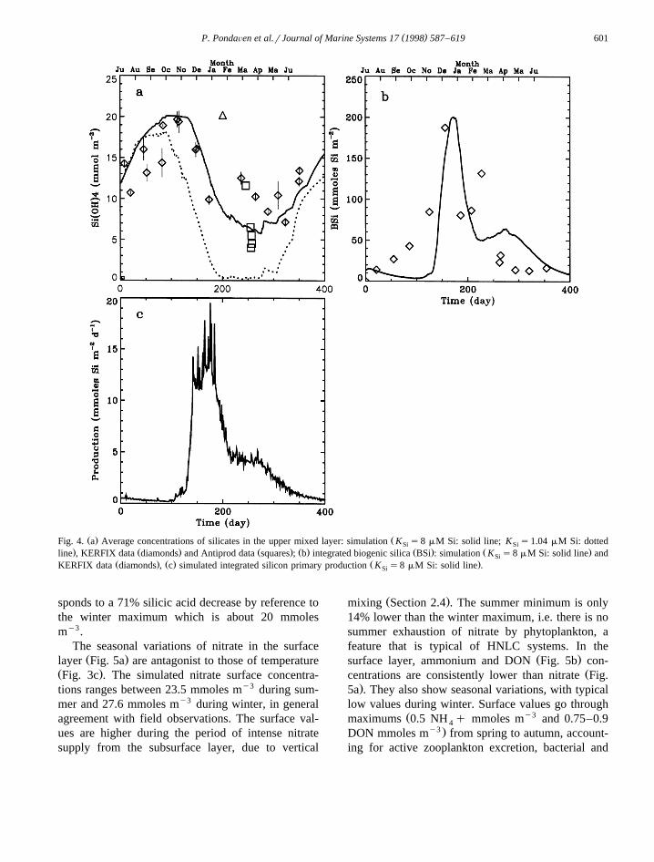
Ž . ŽFig. 4. a Average concentrations of silicates in the upper mixed layer: simulation K s8 mM Si: solid line; K s1.04 mM Si: dottedSi Si. Ž . Ž . Ž . Ž . Ž .line , KERFIX data diamonds and Antiprod data squares ; b integrated biogenic silica BSi : simulation K s8 mM Si: solid line andSi

Ž . Ž . Ž .KERFIX data diamonds , c simulated integrated silicon primary production K s8 mM Si: solid line .Si

sponds to a 71% silicic acid decrease by reference tothe winter maximum which is about 20 mmolesmy3.

The seasonal variations of nitrate in the surfaceŽ .layer Fig. 5a are antagonist to those of temperature

Ž .Fig. 3c . The simulated nitrate surface concentra-tions ranges between 23.5 mmoles my3 during sum-mer and 27.6 mmoles my3 during winter, in generalagreement with field observations. The surface val-ues are higher during the period of intense nitratesupply from the subsurface layer, due to vertical

Ž .mixing Section 2.4 . The summer minimum is only14% lower than the winter maximum, i.e. there is nosummer exhaustion of nitrate by phytoplankton, afeature that is typical of HNLC systems. In the

Ž .surface layer, ammonium and DON Fig. 5b con-Žcentrations are consistently lower than nitrate Fig.

.5a . They also show seasonal variations, with typicallow values during winter. Surface values go through

Ž y3maximums 0.5 NH q mmoles m and 0.75–0.94y3 .DON mmoles m from spring to autumn, account-

ing for active zooplankton excretion, bacterial and


Ž . Ž . Ž .Fig. 5. a Simulated sea-surface concentrations of nitrates and b simulated sea-surface concentrations of ammonium solid line and DONŽ . Ž . Ž . Ž . Ž . Ždotted line ; c profile of ammonium for day 100 solid line , day 170 dotted line , day 241 dashed line and day 360 dotted and dashed

. Ž . Ž . Ž .line ; d production and consumption fluxes of ammonium for day 241: budget solid line , phytoplankton uptake dotted line , bacterialŽ . Ž . Ž .uptake minus release dashed line , zooplankton excretion dotted and dashed line and oxidation 3=dotted and dashed line .

phytoplankton release or detrital breakdown. FromŽ .spring to autumn Fig. 5c , vertical profiles of am-

monium show a subsurface maximum of about 0.49mmoles my3 on day 241, which is a characteristic

Žfeature of the POOZ ecosystem Goeyens et al.,.1991; Queguiner et al., 1997 . This subsurface maxi-´

Ž .mum is explained from the balance Fig. 5d be-Žtween negative ammonium fluxes phytoplankton up-

.take and oxidation processes and positive ammo-Žnium fluxes heterotrophic activity of bacteria and

.zooplankton excretion . Bacteria and microzooplank-ton are especially active to produce or to uptakeammonium in the surface as well as in the subsur-

Ž .face layer Ducklow and Carlson, 1992 . Because theammonium uptake due to phytoplankton is activeonly in the photic layer during spring and summer, at


the base of the photic layer an ammonium maximumŽ .is generated only during this period Fig. 5c and d .

At this depth, the presence of microzooplankton,especially active in generating ammonium, is in partlinked to that of bacteria, a prey for microzooplank-

Ž .ton Fig. 2 .The seasonal variations of the concentrations of

both chlorophyll-a and net primary production, inte-grated in the photic layer, are shown in Fig. 6a,b.

From July, 1st 1990 to June, 30th 1991 chlorophyll-aranges between 5 and 55 mg my2 , in general agree-

Žment with KERFIX data Fig. 6a; Fiala, personal.communication . The primary production ranges be-

y2 y1 Ž .tween 25 and 600 mg C m day Fig. 6b .Compared to the few 14C field data measured duringthe summer period in the Indian sector of the POOZ,the model results are in the upper limit of fieldobservations during the February–March period

Ž . Ž . Ž . ŽFig. 6. a Simulated integrated chlorophyll: total chlorophyll solid line , nanophytoplankton dashed line and microphytoplankton dotted. Ž . Ž . Ž . Ž . Ž .line —KERFIX 1992–1995; Fiala et al., 1998 data diamonds ; b simulated integrated net primary production PP : total solid line ,

Ž . Ž . Ž .nanophytoplankton dashed line and microphytoplankton dotted line ; c simulated sea-surface zooplankton concentration: microzooplank-Ž . Ž . Ž . Ž . Ž .ton dotted line and mesozooplankton solid line ; d simulated sea-surface bacterial concentration dotted line and production solid line .


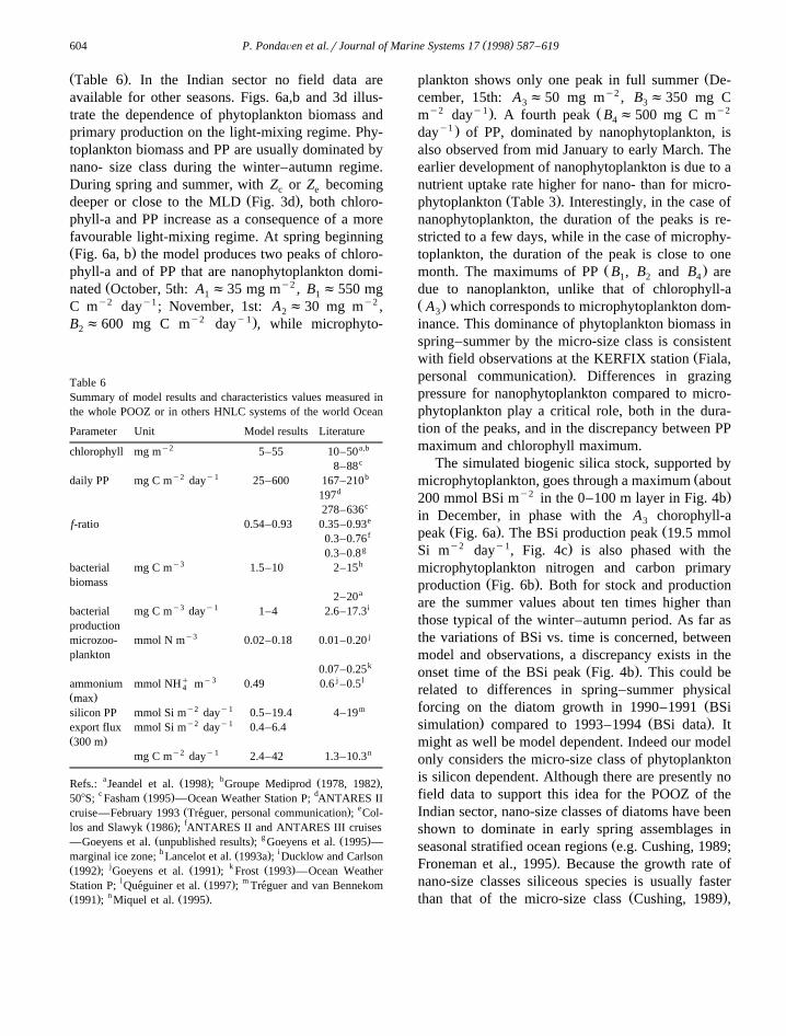
Ž .Table 6 . In the Indian sector no field data areavailable for other seasons. Figs. 6a,b and 3d illus-trate the dependence of phytoplankton biomass andprimary production on the light-mixing regime. Phy-toplankton biomass and PP are usually dominated bynano- size class during the winter–autumn regime.During spring and summer, with Z or Z becomingc e

Ž .deeper or close to the MLD Fig. 3d , both chloro-phyll-a and PP increase as a consequence of a morefavourable light-mixing regime. At spring beginningŽ .Fig. 6a, b the model produces two peaks of chloro-phyll-a and of PP that are nanophytoplankton domi-

Ž y2nated October, 5th: A f35 mg m , B f550 mg1 1

C my2 dayy1 ; November, 1st: A f30 mg my2 ,2y2 y1.B f600 mg C m day , while microphyto-2

Table 6Summary of model results and characteristics values measured inthe whole POOZ or in others HNLC systems of the world Ocean

Parameter Unit Model results Literaturey2 a,bchlorophyll mg m 5–55 10–50

c8–88y2 y1 bdaily PP mg C m day 25–600 167–210

d197c278–636ef-ratio 0.54–0.93 0.35–0.93f0.3–0.76

g0.3–0.8y3 hbacterial mg C m 1.5–10 2–15

biomassa2–20

y3 y1 ibacterial mg C m day 1–4 2.6–17.3production

y3 jmicrozoo- mmol N m 0.02–0.18 0.01–0.20plankton

k0.07–0.25q y3 j lammonium mmol NH m 0.49 0.6 –0.54

Ž .maxy2 y1 msilicon PP mmol Si m day 0.5–19.4 4–19y2 y1export flux mmol Si m day 0.4–6.4

Ž .300 my2 y1 nmg C m day 2.4–42 1.3–10.3

a Ž . b Ž .Refs.: Jeandel et al. 1998 ; Groupe Mediprod 1978, 1982 ,c Ž . d508S; Fasham 1995 —Ocean Weather Station P; ANTARES II

Ž . ecruise—February 1993 Treguer, personal communication ; Col-´Ž . flos and Slawyk 1986 ; ANTARES II and ANTARES III cruisesŽ . g Ž .—Goeyens et al. unpublished results ; Goeyens et al. 1995 —

h Ž . imarginal ice zone; Lancelot et al. 1993a ; Ducklow and CarlsonŽ . j Ž . k Ž .1992 ; Goeyens et al. 1991 ; Frost 1993 —Ocean Weather

l Ž . mStation P; Queguiner et al. 1997 ; Treguer and van Bennekom´ ´Ž . n Ž .1991 ; Miquel et al. 1995 .

Žplankton shows only one peak in full summer De-cember, 15th: A f50 mg my2 , B f350 mg C3 3

y2 y1. Ž y2m day . A fourth peak B f500 mg C m4y1 .day of PP, dominated by nanophytoplankton, is

also observed from mid January to early March. Theearlier development of nanophytoplankton is due to anutrient uptake rate higher for nano- than for micro-

Ž .phytoplankton Table 3 . Interestingly, in the case ofnanophytoplankton, the duration of the peaks is re-stricted to a few days, while in the case of microphy-toplankton, the duration of the peak is close to one

Ž .month. The maximums of PP B , B and B are1 2 4

due to nanoplankton, unlike that of chlorophyll-aŽ .A which corresponds to microphytoplankton dom-3

inance. This dominance of phytoplankton biomass inspring–summer by the micro-size class is consistent

Žwith field observations at the KERFIX station Fiala,.personal communication . Differences in grazing

pressure for nanophytoplankton compared to micro-phytoplankton play a critical role, both in the dura-tion of the peaks, and in the discrepancy between PPmaximum and chlorophyll maximum.

The simulated biogenic silica stock, supported byŽmicrophytoplankton, goes through a maximum about

y2 .200 mmol BSi m in the 0–100 m layer in Fig. 4bin December, in phase with the A chorophyll-a3

Ž . Žpeak Fig. 6a . The BSi production peak 19.5 mmoly2 y1 .Si m day , Fig. 4c is also phased with the

microphytoplankton nitrogen and carbon primaryŽ .production Fig. 6b . Both for stock and production

are the summer values about ten times higher thanthose typical of the winter–autumn period. As far asthe variations of BSi vs. time is concerned, betweenmodel and observations, a discrepancy exists in the

Ž .onset time of the BSi peak Fig. 4b . This could berelated to differences in spring–summer physical

Žforcing on the diatom growth in 1990–1991 BSi. Ž .simulation compared to 1993–1994 BSi data . It

might as well be model dependent. Indeed our modelonly considers the micro-size class of phytoplanktonis silicon dependent. Although there are presently nofield data to support this idea for the POOZ of theIndian sector, nano-size classes of diatoms have beenshown to dominate in early spring assemblages in

Žseasonal stratified ocean regions e.g. Cushing, 1989;.Froneman et al., 1995 . Because the growth rate of

nano-size classes siliceous species is usually fasterŽ .than that of the micro-size class Cushing, 1989 ,


consideration of smaller siliceous species in themodel would have produced a more rapid onset ofthe BSi peak in early spring.

The microzooplankton biomass is lower by aŽfactor of about 2 annual range: 0.02–0.18 mmol N

y3 . Žm , Fig. 6c than that of nanophytoplankton an-y3 .nual range: 0.04–0.50 mmol N m . Because mi-

crozooplankton field data are not available for theIndian sector of the POOZ, we can only compare our

Ž .model results to other HNLC systems Table 6 . Themodel outputs are within the range of observedmicrozooplankton biomasses reported for the At-

Ž .lantic sector of the POOZ Goeyens et al., 1991 orŽ .for the subarctic Pacific Frost, 1993 . Furthermore,

Ž .the microzooplankton biomass peaks Fig. 6c followŽ .those of nanophytoplankton Fig. 6a with a time-lag

of only five days. This short time-lag has to berelated with the fast microzooplankton growth rateŽ .Table 4 , and, as reported on Fig. 6a and c,nanophytoplankton and microzooplankton biomassesshow oscillations that have to be related with preda-tor–prey cycles. This supports the idea that thenanophytoplankton standing stock is mainly control

Žby microzooplankton grazing pressure see Section.4 .

The magnitude of the variations in mesozooplank-Ž .ton biomass Fig. 6c is comparable to microzoo-

Ž y3 .plankton range: 0.02 to 0.22 mmol N m . Themesozooplankton starts to develop when microphy-toplankton crop size is the highest, and, contrary tomicrozooplankton, only one single mesozooplankton

Žbiomass maximum is observed during summer on.January, 20th . These model results are in general

agreement with KERFIX data which show mesozoo-plankton biomass maximum of about 0.10 mmol N

y3 Ž .m occurring in January Razouls et al., 1995 . Thetime-lag between the peak of mesozooplankton andof microphytoplankton is about one month. Com-pared to microzooplankton, this higher time-lag formesozooplankton is explained by a lower specific

Ž .growth rate Table 4 .The bacteria biomass ranges from 0.01 to 0.20

y3 Ž .mmol N m Fig. 6d . This corresponds to 0.5–9mg C my3 by assuming a CrN ratio of 4 for

Ž .bacteria Lancelot et al., 1993b . These results arecompatible with values reported at KERFIX stationŽ y3 .2–15 mg C m , Jeandel et al., 1998 . The simu-

Ž .lated bacterial production Fig. 6d varies between

and 0.05 to 3.5 mg C my3 dayy1 in reasonableagreement with field data for open ocean watersreported in Table 6. The pattern of the seasonal

Žvariations of bacterial biomass and production Fig..6d is out of phase with that of microzooplankton

Ž .Fig. 6c : the maxima of bacteria biomass are ob-served when microzooplankton biomass is the low-est. Bacterial production and biomass increase alsocoincides with that of DON and of ammonium re-ported in Fig. 5b. Still in Fig. 5b, DON and ammo-nium increase during spring and summer responsesto heterotrophs development, via exudation and ex-cretion processes as well as detrital breakdown.

3.3. The production of biogenic matter in the surfacelayer: annual budgets

The model annual estimate for the total produc-tion of particulate organic nitrogen in the POOZ is

y2 y1 Ž .0.85 mole N m year Fig. 2, Table 7 .Nanophytoplankton accounts for 63% of this total,while microphytoplankton accounts for only 37%Ž .Fig. 2 . The corresponding total primary productionis 68 g C my2 yeary1, compatible with CZCS

Ž y2 y1estimations 75–100 g C m year : Antoine etal., 1996; 120–165 g C my2 yeary1 : Longhurst et

.al., 1995 . Interestingly this corresponds to a newproduction of 21 g C my2 yeary1 based on thephotic layer nitrate depletion, which is close to the

y2 y1 Ž .27 g C m year proposed by Jacques 1991 as apreliminary estimate of new production in the POOZIndian sector.

An annual production of biogenic silica of 1.32mol BSi my2 yeary1 in the 0–100 m layer isanother important output of the model. No directvalidation of this estimate is presently possible as noseasonal coverage of the BSi production has beenreported for in the Indian sector, but our estimate isconsistent with values published for other regions of

Ž .the Southern Ocean Table 7 .

3.4. The production regime

Another output of the model are the seasonalvariations of the primary production regime via thef-ratio. This ratio goes through a maximum of 0.93

Ž .during early spring November, 15th and a minimalŽ .value of 0.54 in late summer March, 15th , when


Table 7Ž . Ž . Ž . Ž . y2 y1 y2 y1Annual primary production PP of biogenic silica BSi , nitrogen PON and carbon POC in moles Si m year and g C m year

Ž . y2 y1 y2 y1—assuming a CrN Redfield ratio of 6.625; exportation EF in moles Si m year and g C m year ; EFrPP ratio

Depth BSi PON SirN ratio POC

PP 1.32 0.85 1.6 68a bAustral Ocean 0.9–4.7 16c dCircum Polar current 0.2–3.5 -50a b0.9–4.7 16e f0.4–0.8 3–40

g50–100h120–165

iOcean Weather station P 48–166EF 100 m 0.83 0.14 5.9 11

300 m 0.75 0.06 12.5 4.8500 m 0.63 0.05 12.6 4

eCircum Polar current sediment deposits 0.2j1.36–2.43f f100 m 0.06–0.85 0.09–2.8

EFrPP 100 m 63% 16%300 m 57% 7%500 m 48% 6%

eCircum Polar current sediment deposits 25–40%

Ž .Model results bold and literature data set.a Ž . b Ž . c Ž . d Ž . e Ž .Refs.: Treguer and van Bennekom 1991 , Sakshaug et al. 1991a,b , Nelson et al. 1995 , Jacques 1991 , Leynaert et al. 1993 ,´

f Ž . g Ž . h Ž . i Ž . j Ž .Wefer and Fischer 1991 , Antoine et al. 1996 , Longhurst et al. 1995 , Fasham 1995 , Rabouille et al. 1997 .

biological activity supplies ammonium in surfacelayer. As we can see in Table 6, these variations areconsistent with recent measurements in the study

Žarea during the cruises ANTARES II February,. Ž6th–March, 8th 1994 and ANTARES III Septem-

.ber 28th–November 8th 1995 with f-ratio rangingbetween 0.6–0.76 in early spring and 0.3–0.4 in late

Ž .summer Goeyens et al., unpublished results . Dur-ing summer, if our model is correct, up to 50% ofthe total primary production is recycled production,i.e. sustained by ammonium, in spite of the high

Ž y3 .nitrate pool greater than 23 mmoles m thatremained during this period. Indeed, V y is de-NO3

creased by a factor of 3 in response to increasedammonium availability in late summer. Such largeseasonal variations of f-ratio have already been re-ported for the marginal ice zone, with maximal

Ž .values greater than 0.8 observed at the onset of theŽ .growing period and minimal values ;0.3 in sum-

Ž .mer Goeyens et al., 1995 . Incidently our modelgives an average value of 0.71 on an annual basis,

Žmuch higher than for the MIZ annual average of.0.5"0.2, Goeyens et al., 1995 , showing that the

new production regime finally dominates in thePOOZ at annual scale.

3.5. Exportation Õs. production: the decoupling be-tween N and Si cycles

Ž .Daily average export fluxes DEF of BSi andPOC at 300 m depth are shown on Fig. 7a and b.The simulated ranges for DEF are 0.4–6 mmol Simy2 dayy1 and 0.03–0.53 N mmol my2 dayy1 forbiogenic silica and particulate organic nitrogen, re-spectively. For particulate organic carbon this corre-sponds to an export flux of 2.4–42 mg C my2

dayy1, which is compatible with the DEF measuredin the KERFIX sediment trap at 300 m: 1.3–10.3 mgC my2 dayy1 with a maximum occurring on Jan-

Ž .uary Table 6 . During winter, a period of lowactivity both for microphytoplankton and macrozoo-

Ž .plankton, the simulated DEF at 300 m depth Fig. 7keeps to low values: 0.4–1 mmol Si my2 dayy1 and

y2 y1.0.03–0.05 mmol N m day . These fluxes in-crease during the spring–summer period, as a conse-quence of increasing biological activity, and reach a


Ž . Ž . Ž . Ž .Fig. 7. Monthly average export fluxes out of the 0–300 m layer: a biogenic silica BSi ; b particulate organic nitrogen PON : totalŽ . Ž .export fluxes solid line , phytodetritus and microzooplankton carcasses and faecal pellets D ) and D , dotted line mesozooplankton1 1

Ž .carcasses and fecal pellets D ) and D , dashed line .2 2

Ž .maximum in January Fig. 7 . This DEF peak ismainly supported by mesozooplankton faecal pelletsproduction, in phase with the maximum of mesozoo-plankton biomass of Fig. 6c. In addition, it is ob-served that the export flux sustained by mesozoo-plankton detritus accounts for 62% and 86%, for BSiand PON, respectively. Finally, 87% of the annualexport flux occurs during the period from October,1st to March, 30th.

Illustrating the importance of the silica pump inthe Southern Ocean, silicon and nitrogen show adifferent behaviour. As reported in Table 7, thesimulated annual export fluxes of BSi and PON havebeen calculated at 100 m, 300 m and at the bottom of

Ž .our model 500 m . At 500 m depth, the exportfluxes are 0.63 mol Si my2 yeary1 and only 0.06

y2 y1 Ž y2 y1.mol N m year 4.8 g C m year . Thesefluxes represent 48% of the BSi and 6% of the PONthat is produced in the photic layer; the rest beingregenerated in the 0–500 m layer. Consequently, inthe photic layer the SirN molar ratio of the produc-tion fluxes is 1.6, while at 500 m depth the SirNmolar ratio of the export fluxes is one order of

Ž .magnitude higher: 12.6 Table 7 . This suggests thatnitrogen is rapidly regenerated in surface compared

to silicon. From in vitro experiments conductingduring summer in the POOZ of the Indian sector

Ž .Treguer et al. 1989 showed that the specific disso-´lution rate of BSi range between 0.007 and 0.017

y1 Ž y1 .day 0.012 day in our model . This is one orderof magnitude lower than the specific rate of nitrogen

Ž y1recycling about 0.05–0.23 day measured by.Sempr et al., unpublished results in the same region

and season.The simulated export fluxes are dependent on the

detritus sinking rates. Thus, if the sinking rate ofsmall detritus decreases from 5 m dayy1 to 1 mdayy1, the annual export flux at 500 m is decreasedby a factor 3 compared to the values given in Table7. The processes that control the pathways of trans-porting the particulate organic matter throughout thewater column, also important to constrain the model,are still poorly documented in the study area. Forexample, salps can play a major role in export fluxesvia the production of high sinking rates faecal pelletsŽ .Andersen and Nival, 1988 . Being unselective filtersthey ingest living phytoplankton and detritus as well,and they packaged material settled down at very high

y1 Žsinking rates, greater than 1000 m day Bruland.and Silver, 1981 . Likewise, aggregation processes


Fig. 8. Simulated mixed layer depth for the 1990–1991 periodŽ . Ž .solid line and the 1991–1992 period dotted line , from 1st Julyto 30th June.

of algal cells which usually follow a diatom bloom—a process which is not taken into account here—could also significantly affect export fluxes. Indeed,diatoms aggregates can sink at rates greater than 100

y1 Ž .m day Alldredge and Gotschalk, 1989 .

3.6. SensitiÕity analysis-Õariability in the light-mix-ing regime

To determine the key parameters that control themodel behaviour, a sensitivity analysis has been

performed. The method and the results of this analy-sis are given in Appendix B. In short, the sensitivityanalysis shows that the state variables are mainlysensible to phytoplankton, zooplankton and bacteria

Žgrowth parameters e.g. nutrients uptake rates and.ingestion rates , which are, for most of them, body-Ž .size dependent Section 2.3 .

It has been previously reported that the date of theobserved chlorophyll maximum can vary from oneyear to another of about one month. To investigatethe impact of interannual variations in meteorologi-cal conditions on biology, the model has been run forthe conditions prevailing in 1991–1992, with physi-cal forcings different from those used for the stan-

Ž .dard run 1990–1991 . As shown in Fig. 8, a signi-ficative interannual variability in the MLD appears

Ž .between the two years. For year 1 1990–1991 themean summer MLD is closed to 50–70 m, while in

Ž .year 2 1991–1992 , the mean summer MLD isconsistently deeper—about 90–100 m. Further, thestratification of the water column occurs three months

Ž .later during year 2 on January 1st than during yearŽ .1 on October 1st . This interannual variability of

MLD significatively affects the general behaviour ofthe whole biogeochemical model, as shown by Table8. The chlorophyll maximum, mainly due to micro-phytoplankton, occurs one month later in year 2compared to year 1, but its concentration is now 76mg Chl-a my2 , that is significantly higher than for

Ž y2 .the standard run 55 mg Chl-a m . This high year

Table 8ŽSummary of model results obtained with two different physical forcing i.e July 1st 1990–June 30th 1991 and July, 1st 1991–June, 30th

.1992

Variables 1990–1991 1991–1992 Unit

mean MLD 64 92 my2Chlorophyll maximum 55 76 mg Chl-a m

date December 15th January 12th –y2 y1PP total Si 1.32 1.01 mol Si m yeary2 y1total N 0.85 0.68 mol N m yeary2 y1microphyto- 0.26 0.23 mol N m yeary2 y1nanophyto- 0.59 0.45 mol N m yeary2 y1EF Si 0.62 0.56 mol Si m yeary2 y1C 0.05 0.02 mol N m year

y3Ž .Si OH 4 9 11 mmol Si mminy y3NO3 22 24 mmol N mmin

Average spring–summer MLD—from October 1st to March 15th; magnitude and date of the chlorophyll maximum; Primary ProductionŽ . Ž . Ž Ž . .PP for silicon and nitrogen; Export Flux EF out of the first 500 m; summer minimal concentration of silicate Si OH 4 and nitrateminŽ y .NO3 .min


2 chlorophyll maximum is determined by a MLD asŽ .shallow as 40 m during a 16-day period Fig. 8 .

Nevertheless, the total annual PP decreases by 15%from year 1 to year 2, both for microphytoplankton

Ž .and nanophytoplankton Table 8 .

4. Discussion

In the fifty degrees of latitude both the SouthernOcean and the North Atlantic are typical seasonallystratified areas. In these stratified areas the earlyspring bloom classically starts by the outburst ofsmall diatoms. As the stratification of the watercolumn goes on, larger diatoms grow up. Then dur-ing late spring and summer, when the stratification is

Žmaximum, dinoflagellates predominate Cushing,.1989 . Such algal successions have effectively been

observed in the North Atlantic with characteristicspring blooms greater than 3 mg Chlya my3 due to

Ž .microphytoplankton Lochte et al., 1993 . Howeverblooms of the same magnitude have never beenobserved in the POOZ of the Southern Ocean. Thusthe question is: what is so different in the POOZ ofthe Southern Ocean compared to the North Atlantic,that prevents diatoms from blooming?

Grazing pressure has been suggested to play acritical role in the control of phytoplankton standing

stocks in HNLC systems such as the equatorialŽ .Pacific Frost and Franzen, 1992 , the subarctic Pa-

Ž .cific Evans and Parslow, 1985; Fasham, 1995 , andŽthe MIZ of the Southern Ocean Lancelot et al.,

.1993b . If our model is correct, during the growingŽ .period from mid-October to April , the microzoo-

plankton grazing pressure in the POOZ accounts for35% to 100% of daily nanophytoplankton primary

Ž . Ž .production DNPP Fig. 9a , and for 70% of DNPPon an annual basis. The other loss terms, exudationand mortality, are less important, only accounting for5–25%. So, the high grazing pressure explains, byitself, the lack of nanophytoplankton bloom during

Ž .spring–summer Fig. 6a . During the North AtlanticŽ .Bloom Experiment NABE , in the post-bloom pe-

riod, microzooplankton has been shown to graze upto 100% of the daily phytoplankton productionŽ .Ducklow and Harris, 1993 . Our model demon-strates that the seasonal increase in algal biomass canonly be achieved in the POOZ by microphytoplank-

Žton. Field observations Fiala, personal communica-.tion actually show that the microphytoplankton size

class is the major contributor to the seasonal chloro-phyll a maximum. Nevertheless, this maximum inthe POOZ never exceeds 1.5 mg my3, a value that isat least two times lower than for the Atlantic OceanŽ .Lochte et al., 1993 . During the first part of the

Ž .growing period from day 100 to day 170 in Fig. 9b ,

Ž . Ž . Ž .Fig. 9. a Daily nanophytoplankton gross primary production thin line , exudation and mortality bold line and microzooplankton grazingŽ . Ž . Ž . Ž .pressure dotted line ; b daily microphytoplankton gross primary production thin line , exudation and mortality bold line , mesozooplank-

Ž .ton grazing pressure dotted line . The fluxes have been integrated over the first 50 m.


mesozooplankton grazing pressure only account for2–40% of daily microphytoplankton primary produc-

Ž .tion DMPP . During this period, the main loss termsare mortality and exudation which account for 15–45% of DMPP. During the second part of the grow-

Ž .ing period from day 170 to day 250 , mesozoo-plankton grazing pressure becomes the main lossterm, accounting for 40–95% of DMPP. This graz-ing pressure induces the collapse of the chlorophyllmaximum shown in Fig. 6a. Averaged over thewhole year, mesozooplankton exerts a moderatepressure on microphytoplankton in the POOZ, onlyaccounting for 27% of the DMPP. Heterotrophicactivity measurements during NABE shown thatmesozooplankton cannot graze more than a few per-cent of the daily primary production. Finally as far asthe grazing pressure is concerned, the North Atlanticand the Southern Ocean follow the same pattern.

Another hypothesis which might be a key causeŽof HNLC areas is the shallow winter MLD Evans

.and Parslow, 1985; Fasham, 1995 . Indeed, the shal-low winter MLD, which is typical of the equatorialand subarctic Pacific HNLC areas, allows a winterprimary production sufficient to sustain a winterzooplankton standing stock large enough to preventphytoplankton from blooming at the onset of thegrowing period. On the contrary, the deep winter

Ž .MLD observed in the North Atlantic G300 mleads to a low winter zooplankton stock which is notable to prevent phytoplankton from blooming at theonset of the growing period. In the POOZ, the winter

Ž .MLD is closed to 200 m Fig. 3d , that is shallowerthan in the North Atlantic. Therefore, the question is:is the winter MLD in the POOZ shallower enough tosustain a winter zooplankton standing stock largeenough to prevent phytoplankton from blooming inspring? In order to investigate this question, we haverun the model with a winter MLD close to 300 m, bytuning the eddy diffusivity coefficient between day 0and day 100. Results, displayed on Fig. 10, showthat the winter MLD reaches 300 m in late Septem-ber. It should be noted that the deepening of the

ŽMLD during winter does not affect the SST figure.not shown . In addition, after day 100, the MLD

finds again the values characteristics of the standardrun observed in Fig. 10a. On Fig. 10b, we haveplotted the seasonal course of chlorophyll a andsilicic acid for the standard run and for the run witha winter MLD of order 300 m. Deepening the winterMLD does not affect significantly the seasonal courseof the plankton cycle. Although the winter chloro-phyll remains lower than in the standard run betweenday 0 and day 100, the chlorophyll maximum isclosed to the standard run value with a maximum of

Ž . Ž . Ž .Fig. 10. a Seasonal course of the mixed layer depth MLD : standard simulation solid line and simulation with a winter MLD close toŽ . Ž . Ž .300 m dotted line ; 10b seasonal course of 0–50 m integrated chlorophyll a and nitrates for the standard simulation solid line and for the

Ž .simulation with a winter MLD of order 300 m dotted line .


54 mg Chl-a my2 . As shown by Fig. 10b, the wintermaximum of silicic acid in surface water in higherthan in the standard run. As a consequence, silic acidlimitation on microphytoplankton primary produc-tion is lower, so that total primary production in-creases from 68 g C my2 yeary1 in the standard runto 74 g C my2 yeary1. In short, in spite of a higherprimary production, no bloom is observed when thewinter MLD is of order 300 m. Therefore, we canhypothesize that in the POOZ, nanophytoplankton isclearly kept from blooming because of microzoo-plankton grazing pressure. But for microphytoplank-ton, in our model, deep winter MLD does not drivethe pattern of the spring–summer microphytoplank-ton dynamic. Therefore, the HNLC feature of thePOOZ might be control by factors that act duringspring–summer period.

To determine the specific contribution of thelight-mixing regime in the control of the photosyn-thetic activity in the POOZ we have run the model

Ž .with no Si limitation Table 9 . The physical forcingbeing identical to that of the standard run, when KSi

is put to 0 mmoles my3, the spring–summer nitrateminimum decreases from 23.5 to 21.6 mmoles Nmy3. While the chlorophyll maximum grows upfrom 1.08 to 2.2 Chl-a mg my3, the annual primaryproduction rises up to 86 g C my2 yeary1, that is

Ž y227% higher than for the standard run 68 g C my1 .year . Nonetheless this is still about three times

lower than the 240 g C my2 yeary1, typical of theNorth Atlantic for the same latitudinal bandŽ .Longhurst et al., 1995 . In stratified antarctic MIZwaters, when the MLD becomes smaller than 25 m

Table 9Summary of model results obtained by assuming no silicateslimitation

Variable Value Unit

MLD 63.9 my2Chl-a 109 mg mmax

yNO3 21.6 mMmin

f-ratio 0.74y2 y1PP 111 g C m yeary2 y1Ž .EF 100 m 12 g C m year

Average spring–summer MLD—from October 1st to March 15th;magnitude and date of the chlorophyll maximum; summer mini-

Ž y .mal concentration of nitrate NO3 ; f-ratio; Primary ProductionminŽ . Ž .PP ; Export Flux EF out of the first 100 m.

during sea–ice retreat conditions, Mitchell andŽ .Holm-Hansen 1991 observed blooms with chloro-

y3 Žphyll values greater than 10 mg m see also.Goosse and Hecq, 1994 . Likewise, in the North

Atlantic, when the MLD is smaller than 30 m,phytoplankton blooms with chlorophyll values greaterthan 3 mg Chl-a my3 and primary production rang-ing between 600–1800 mg C my2 dayy1 have also

Ž .been evidenced, during summer Lochte et al., 1993 .This suggests that the typical spring–summer MLD

Ž .in the POOZ usually greater than 60 m is deeper bya factor of 2 to 4 than that which allows occurrence

Žof phytoplankton blooms Mitchell and Holm-Han-sen, 1991; Nelson and Smith, 1991; Sakshaug et al.,

.1991a . Finally, during the spring–summer period amajor difference between the POOZ of the SouthernOcean and the North Atlantic comes from theirlight-mixing regimes. The Southern Ocean has to be

Žconsidered mainly as a light-limited domain Dug-.dale and Wilkerson, 1991 . By itself however, this

‘unfavourable’ spring–summer light-mixing regimeis not sufficient to explain the whole HNLC features

Ž .of the studied area. Armstrong 1994 , who built amodel with multiple phytoplankton–zooplankton

Žfood chains each food chain being based on a.different size class of algae noted that in HNLC

areas ‘‘high ambient nutrient concentrations duringthe growing season must be due to low growthrates . . . or high half-saturation constants of the nexthigher . . . phytoplankton size class’’, suggesting nu-trients may also play a role in controlling the micro-phytoplankton development.

Our model accounts for the seasonal field varia-tions of phytoplankton stocks and fluxes by takinginto account of low V and V . Dugdale andNO3 Si

Ž .Wilkerson 1991 observed that HNLC systems arecharacterized by V that are systematically lowerNO3

than expected, with regards to the high availableŽ y1 .nitrogen pool range 0.027–0.056 day . To ex-

plain such low values they envisaged different hy-Ž . Ž .pothesis: 1 grazing control, 2 strong meteorologi-

Ž .cal conditions and light-mixing regime control, 3Ž . Ž .ammonium inhibition, 4 temperature limitation, 5

Ž .iron limitation, and finally 6 silicic acid limitation.As shown above, grazing and light-mixing regimecontrols are certainly involved but cannot explain thewhole story. Our model produces maximal concen-trations of ammonium close to 0.4–0.6 mmoles


y3 Ž .N m , which according to Lancelot et al. 1993bŽ .see Appendix A leads to a decrease of V by aNO3

Ž .maximal factor of 3. Dugdale and Wilkerson 1991advanced temperature ‘may be sufficient to deter-mine the HNLC nature of the Southern Ocean’.

Ž .However, Jacques 1983 showed that N. kerguelen-sis, a diatom typical of the POOZ, reaches its opti-mal growth rate at ;5–88C, i.e. for a temperature

Ž .close to the characteristic summer SST Fig. 3c . Wethus run our model with the assumption that thesiliceous phytoplankton is well adapted to low tem-peratures. Ultimately, to reproduce the HNLC fea-tures of the studied area a nutrient limitation has tobe taken into account. A major difference that distin-guishes the POOZ of the Southern Ocean from theNorth Atlantic is the importance of its inorganicnutrient pool, at the onset of the growing period. Inthe POOZ, nitrate and silicic acid concentrationsŽ y3 y3.;28 mmoles N m and ;20 mmoles Si mare higher by a factor of 3 to 5 than the values

Ž .reported by Lochte et al. 1993 for the North At-Ž y3lantic ;7 mmoles N m and ;4 mmoles Si

y3 .m , leading to potential dense phytoplanktonblooms. In the North Atlantic nitrate and silicic acidconcentrations fall below 1 mmoles my3 by late

Ž .spring Lochte et al., 1993 . Referring to usual val-ues for the half-saturation constants of both nitrate

Žand silicic acid uptake rates Eppley et al., 1969;.Nelson and Treguer, 1992 , it is clear that such low´

nutrient concentrations in surface waters can limitboth the growth of diatoms and that of other nonsiliceous species. In the POOZ, although the silicicacid summer decrease is twice higher than in thenorth Atlantic, both nitrate and silicic acid are never

Ž y3exhausted minimum of ;23 mmoles N m andy3 .;6 mmoles Si m . This suggests that the primary

production should not be limited by macronutrientsin this area, leading to focused attention on micronu-

Ž .trients such as iron Martin, 1991 . For the equatorialŽ .Pacific, Armstrong 1994 in his multiple food chain

model, had to decrease the maximum specific nutri-ent uptake rates of microphytoplankton to accountfor a trace metal limitation. For the Southern Ocean

Ž .DeBaar et al. 1995 proposed that iron effectivelylimits primary production, at least in the Atlanticsector in the frontal zone and in the POOZ. Nonethe-

Žless available data in the Indian sector Sarthou et.al., 1995 does not support this iron hypothesis and

our model assumes a silicic acid limitation of micro-phytoplankton growth by increasing the K of sili-Si

cic acid uptake up to 8 mmoles Si my3. As notedabove, K values higher than 2–3 mmoles Si my3

SiŽare quite unusual for marine ecosystems Nelson and

.Treguer, 1992 . However half-saturation constant´values as high as 12–22 mmoles Si my3 have beenreported for two diatoms species collected in the

Ž .POOZ Jacques, 1983 , and much higher values haveŽ .even been measured by Sommer 1986, 1991 for

antarctic assemblages in the seasonal ice zone. Fig.11 shows that K can be related to ambientSiw Ž . xSi OH . Generally speaking, K increase as am-4 Si

w Ž . xbient Si OH increase, and, the highest values—up4

to ;17–88 Si mmoles my3 —are found in Antarcticsilic acid enriched waters. As mentioned by Nelson

Ž .and Brzezinski 1990 , K could reflect geneticSi

adaptations to silicic acid enriched or depleted envi-ronments; adaptations which then induce interspe-cific and intraspecific variability in silicon uptakekinetics. Although no direct validation of the sea-

w Ž . xFig. 11. Relationship between the ambient Si OH and the4Ž .half-saturation constant for silicic acid uptake K of diatomsSi

communities for different types of ecosystems. Refs.: IndianŽ . Žsector of the Southern Ocean )Jacques, 1983 , Ross Sea Nelson

.and Treguer, 1992 , Drake passage and N–E Weddell Sea´Ž . Ž .)Sommer, 1986 , Antarctic Peninsula )Sommer, 1991 , Gulf

Ž . ŽStream Nelson and Brzezinski, 1990 , Peru upwelling Goering et. Žal., 1973; Nelson et al., 1981 ; California Gulf Azam and Chisolm,

.1976 . ) Note that solid lines does not represent error bars but theamplitude of variability. Indeed these points are related to siliconuptake kinetics studies made on monospecific cultures; and we

Ž .have calculated the average K diamonds .Si


sonal variations of V given by the model isSi

presently possible, the uptake rates our model calcu-late for the end of the summer period are in agree-

Ž y1 .ment with the first values of V -0.04 daySiŽever measured in the study area by Caubert et al. in

.preparation .

5. Conclusion

In conclusion, our model helps pointing out theparallels and the contrasts between the 508 latitudinalband of the North Atlantic and the POOZ of theSouthern Ocean. For both systems the nanophyto-plankton dynamic is controlled by microzooplanktongrazing. Spring–summer blooms are specially due tomicrophytoplankton. In spite of high nutrient concen-trations in the POOZ in the early spring, paradoxi-cally the growth of antarctic diatoms seems also tobe silicic acid limited, and similarly to the NorthAtlantic. What is finally different is the very deepspring–summer MLD that prevents the antarctic mi-crophytoplankton from blooming.

Acknowledgements

We express our sincere gratitude to the scientificco-ordinators of the KERFIX programme, A. Pois-

Ž . Ž .son up to 1992 and C. Jeandel since 1993 , whomade this research possible. Volunteers from theScientific Base of the Kerguelen Islands carried outthe field work. We thank M. Fiala and A. Leynaertfor providing the chlorophyll and BSI data presentedhere. We thank Meteo France for providing ECMWF´ ´forcings. We also thank two anonymous reviewersfor their helpful comments. This work is part of theJGOFS-France program and was supported by theCentre National de la Recherche Scientifique and theInstitut des Sciences de l’Univers.

Appendix A. Biological processes

A.1. Phytoplankton growth processes nutrient uptakeN1 N 2 ( y 1)rate, m and m unit, sP1 P1

Ž .The dimensionless function f x that describedthe dependence of phytoplankton uptake rate on light

Ž .availability is taken from Morel 1991 . This func-tion is written:

f x s 1yexp x expyb xŽ . Ž .where b is the photoinhibition parameter. The di-mensionless term x is defined as,

PURxs

KPUR

In this equation, the photosynthetic usable radiation,Ž y2 y1.PUR Einst m s , depends on time, depth,

pigment concentration and temperature. It is normal-ized by the scaling irradiance term KPUR whichdepends on the temperature according to a van’t

Ž .Hoff dependency Morel, 1991 :

KPURsKPUR T c ŽTyT0 .Ž .0

Ž .where KPUR T is the irradiance at which the0Ž .function f x s1r2 for the optimal temperature T .0

Finally, c is the shape factor of the temperaturecurve.

The Photosynthetic Usable Radiation, PUR, islinked to the Photosynthetic Available Radiation,PAR, as follows:

a lŽ .700PURs PAR l dlŽ .H

a )400 max

Where 400–700 nm is the spectral domain of theŽ .PAR and a l represents the chlorophyll specific

Ž 2 y1.absorption spectrum of algae m mg Chl-a ;Ž .a ) is the maximal value found in the a lmax

Ž .spectrum generally at 440 nm .The effect of light mixing regime has been intro-

duced in the model through the dimensionless termŽ .L Andre, 1990 . This term considers simultane-´m

ously the mixed layer depth MLD and the photicŽ .layer depth Z 1% of sea surface irradiance . Thee

Ž .MLD is defined in Gaspar et al. 1990 . Below thephotic layer, L s0, and this coefficient varies be-m

tween 0.5 and 1 above the photic layer. If the mixedlayer depth is twice the photic layer depth thenL s0.5. If the mixed layer is shallower than them

photic layer then L s1, and otherwise, L sm m

Z rMLD.e

The dependence of phytoplankton nutrient uptakerate on nutrient uptake rate is described with aMichaelis–Menten function. Following Wheeler and


Ž .Kokinakis 1990 , the uptake of nitrate decreases asammonium availability increases in the medium. This

Žfeature can be defined as an inhibition effect Fasham.et al., 1990 or a relative preference for ammonium

Ž .Lancelot et al., 1993b . In this study, to allowphytoplankton to take up ammonium preferentially,

Ž .the parameterization of Lancelot et al. 1993b hasbeen adopted. It is described as:

dN N2 2f sg q 1ygŽ .N2 ž /N Ntot tot

where gsy0.21 and ds0.20.

The term N represents the total inorganic nitrogentot

pool, and N is the ammonium concentration. The2

parameter has been adjusted to produce a seasonalŽcourse of f-ratio the fraction of primary production

.due to nitrates that is compatible with field observa-Ž .tions in the studied area see Table 6 .

A.2. Zooplankton growth processes G P1, G B , G P 2Z1 Z1 Z2

Z2 ( y 1)and G unit, sZ1

The specific grazing rates of microozooplanktonand mesozooplankton are adapted from Fasham et al.Ž .1990 . These terms are dependent on food availabil-ity accordingly to a Michaelis–Menten function in-cluding a zooplankton preference coefficient for eachtype of prey. For example, the grazing rate of micro-zooplankton on nanophytoplankton is written as:

GP1 s fP with fsmin Gmax ,G A1Ž .Ž .Z1 1 1 1

The specific filtration rate, f , depends on food avail-ability. It varies between a maximum specific filtra-tion rate of microzooplankton, Gmax and a1

Michaelis–Menten term type, G calculated as:1

IG sg A2Ž .1 1 K qFZ1

In this definition, g is the maximum specific graz-1

ing rate of microzooplankton, K is the half-satura-Z1

tion constant for grazing and I is a dimensionlessfactor representing the preference of microzooplank-ton for nanophytoplankton. This last term is writtenas:

p PP 1Is A3Ž .

p P qp BP 1 B

where p and p measure the microzooplanktonP B

preference for nanophytoplankton and bacteria re-spectively. Finally, F is the total amount of foodavailable for microzooplankton, that is,

Fsp P qp B A4Ž .P 1 B

The grazing rate of microzooplankton on bacteria isparameterized in the same way. The state variable B

Ž . Ž . Ž .replaces P in Eqs. A1 and A2 ; and in Eq. A31

the numerator p P is replaced by p B.P 1 B

Nd N 2 (A.3. Bacterial growth processes m and m unit,B By 1)s

The specific uptake rates of bacteria are depen-dent on resource availability, accordingly to a

ŽMichaelis–Menten function from Evans, in Fasham.et al., 1990 . They are written as:

NdN2 maxm sV f TŽ .B B K qSqNn d

SN2 maxm sV f TŽ .B B K qSqNn d

In these equations, V max is the maximum specificB

nutrient uptake rate, S is the total bacterial nitroge-nous substrate and K the half-saturation constantn

for nutrient uptake. The term S is described as:

Ssmin N ,hNŽ .2 d

where h is the ratio of bacterial ammonium to DONuptake. The bacterial uptake of ammonium and DONis dependent on temperature through the dimension-

Ž .less function f T , taken from Lancelot et al.Ž .1993b :

2T y T Bž /dTf T s0.1q0.9 expŽ .

In this formulation, T is the simulated tempera-ture, T the bacterial growth optimal temperatureB

and dT the shape factor of the temperature curve.

Appendix B. Sensitivity analysis

For the sensitivity analysis, each parameter wasvaried from "10% around the standard value. Then


a quantitative estimate of the normalized sensitivity,IS, has been computed in a similar way than Fasham

Ž .et al. 1990 :

nsX yXÝ i i1 is1ISs is1, n daysn

p sXÝ iis1

In this definition, X s is the concentration of thei

variable X integrated on the first 500 m, for the day

i in the standard simulation. X is the concentrationi

of the variable X, for the day i when one of theparameter has been altered. p is the percentage of

Ž .variation of the parameter i.e. 10% .Table 10 liststhe parameter for which the change in parametervalue involve a value of IS greater than 0.5% for atleast one of the state variable. It appears that, con-cerning phytoplankton parameters, the model is sen-sitive to the maximum nutrients uptake rates, V i

max

the half saturation constant for silicate uptake.Change in those parameters involve IS values greater

Table 10Ž . Ž .Sensitivity of each variable first line for a variation of "1% of each parameter first column

P P Z Z B D D N N N P ) D ) D ) S1 2 1 2 1 2 1 2 d 2 2 2 i

Phytoplankton parametersP1V q )) – – – )) )) ) – )) – – – )) –max

– )) – – – )) )) )) – )) – – – – –P2V q – – – )) )) – )) – )) )) ) ) ) –max

– – ) – – – – ) – – – ) ) ) –Chla: C q – – – )) )) – )) – )) )) – – – –

– )) )) – )) )) )) )) – )) )) – – – –SiV q – – – – – – – – – – )) )) )) ))max

– – – – – – – – – – – )) – – ))

K q – )) – – – – ) – – – )) )) )) ))Si

– – )) – – – – )) – – – )) )) )) ))

Zooplankton parameters1G q )) – )) – ) )) – – – ) – – – –max

– )) – )) )) ) )) – – – ) – – – –2G q – )) )) – – – )) – – )) )) – )) –max

– – – )) )) – – – – – ) )) – )) –g q )) – )) )) )) – – – – – – )) – –1

– – – – – )) – – – – )) – – – –g q – )) )) )) – – )) – – )) )) – )) –2

– – – – )) – – – – – – )) – – –

Bacteria parametersmaxV q – – – – – – – – – ) – – – –B

– – – – – – – – – )) ) – – – –d q – – – – ) – – – )) ) – – – –B

– – – – – )) – – – ) )) – – – –

Mortality and regeneration parametersm q – – – – – )) – – – – – – – –P1

– – – – – – – – – – – – – – –m q – )) – – – )) – – – – – – )) –P2

– – – – – – )) – – – – – – )) –m q )) – – – – )) – – – – – – – –Z1

– – – )) – – )) – – – – – – – –m q – – – – – – )) – – – – – – –Z2

– – – )) – – )) – – – – – – – –

Ž .Relative value of sensitivity index IS : –: IS-0.5%; )): 0.5%-1%; ): IS)s1%.


than 0.5% for several state variables. Concerning thezooplankton parameters, the most sensitive parame-

Ž i .ter are the maximum filtration rates G and themaxŽ .maximum ingestion rate g . Changes in these pa-i

rameters affect both nano- and microphytoplankton,the two size classes of zooplankton, bacteria, DON

Ž .and detritus IS greater than 0.5% . The variation ofbacterial parameters V B and d , respectively themax B

maximum nutrient uptake rate and the assimilationefficiency, also affects several state variables, espe-

q Žcially bacteria, NH4 and DON IS greater than.1% . Mortality parameter values affect especially the

Ž .detrital state variable, D and D ) 0.5%-1% .1 1

Finally, state variables are less sensible to the sink-ing rates when those one are varied from the stan-

Ž .dard value of 1% IS-0.5% .

References

Admiral, W., Peletier, H., Laane, R.W.P.M., 1986. Nitrogenmetabolism of marine planktonic diatoms; excretion, assimila-tion and cellular pools of free amino acids in seven specieswith different cell size. J. Exp. Mar. Biol. Ecol. 98, 241–263.

Alldredge, A.L., Gotschalk, C.C., 1989. Direct observations of themass flocculation diatom blooms: characteristics, settling ve-locities and formation of diatom aggregates. Deep-Sea Res.36, 159–171.

Andersen, V., Nival, P., Harris, R.P., 1987. Modelling of aplanktonic ecosystem in an enclosed water column. J. Mar.Ass. U.K. 67, 407–430.

Andersen, V., Nival, P., 1988. A pelagic ecosystem model simu-lating production and sedimentation of biogenic particles: roleof salps and copepods. Mar. Ecol. Prog. Ser. 44, 37–50.

Andersen, V., Nival, P., 1989. Modelling of phytoplankton popu-lation dynamics in an enclosed water column. J. Mar. Biol.Ass. U.K. 69, 625–646.

Andre, J.M., 1990. Teledtection spatiale de la couleur de la mer:´ ´ ´algorithme dinversion des mesures du Coastal Zone ColorScanner. Applications a l’etude de la Mediterranee occiden-` ´ ´ ´tale. PhD, Universite Pierre et Marie Curie, Paris VI.´

Antoine, D., Andre, J.M., Morel, A., 1996. Oceanic primary´Žproduction: 2. Estimation of global scale from satellite coastal

.zone color scanner chlorophyll. Global Biogeochem. Cycles10.

Armstrong, R.A., 1994. Grazing limitation and nutrient limitationin marine ecosystems: steady state solutions of an ecosystemmodel with multiple food chains. Limnol. Oceanogr. 39, 597–608.

Azam, F., Chisolm, S.W., 1976. Silicic acid uptake and incorpora-tion by natural marine phytoplankton populations. Limnol.Oceanogr. 21, 427–435.

Bruland, K.W., Silver, M.W., 1981. Sinking rates of faecal pellets

Ž .from gelatinous zooplankton salps, pteropods, doliolids . Mar.Biol. 63, 295–300.

Brzezinski, M.A., 1992. Cell-cycle effects on the kinetics ofsilicic acid uptake and resource competition among diatoms. J.Plankton Res. 14, 1511–1539.

Chan, A.T., 1980. Comparative physiological study of marinediatoms and dinoflagellates in relation to irradiance and cellsize: II. relationship between photosynthesis, growth, and car-bonrchlorophyll a ratio. J. Phycol. 16, 428–432.

Collos, Y., Slawyk, G., 1986. 13C and 15 N uptake by marinephytoplankton: IV. Uptake ratios and the contribution of ni-

Žtrate to the productivity of Antarctic waters Indian Ocean.Sector . Deep-Sea Res. 33, 1039–1051.

Conway, H.L., Harrison, P.J., 1977. Marine diatoms grown inchemostats under silicate or ammonium limitation: IV. Tran-sient response of Chaetoceros debilis, Skeletonema costatum,and Thalassiosira graÕida to a single addition of the limitingnutrient. Mar. Biol. 43, 33–43.

Conway, H.L., Harrison, P.J., Davis, C.O., 1976. Marine diatomsgrown in chemostats under silicate or ammonium limitation:II. Transient response of Skeletonema costatum to a singleaddition of the limiting nutrient. Mar. Biol. 35, 187–199.

Coats, D.W., Harding, L.W. jr, 1988. Effect of light history on theultrastructure and physiology of Prorocentrum Mariae-

Ž .Lebouriae Dinophyceae . J. Phycol. 24, 67–77.Cushing, D.H., 1989. A difference in structure between ecosys-

tems in strongly stratified waters and in those that are onlyweakly stratified. J. Plankton Res. 11, 1–13.

Davis, C.O., 1976. Continuous culture of marine diatoms undersilicate limitation: II. Effect of light intensity on growth andnutrient uptake of Skeletonema costatum. J. Phycol. 12, 291–300.

Davis, C.O., Breitner, N.F., Harrison, P.J., 1979. Continuousculture of marine diatoms under silicon limitation: 3. A modelof Si-limited growth. Limnol. Oceanogr. 23, 41–52.

DeBaar, H.J.W., de Jong, J.T.M., Bakker, D.C.E., Lscher, B.M.,Veth, C., Bathmann, U., Smetacek, V., 1995. Importance ofiron for plankton blooms and carbon drawdown in the South-ern Ocean. Nature 373, 412–415.

Ducklow, H.W., Carlson, C.A., 1992. Oceanic bacterial produc-tion. Adv. Microbial Ecol. 12, 113–181.

Ducklow, H.W., Harris, R.P., 1993. Introduction to the JGOFSnorth atlantic bloom experiment. Deep-Sea Res. II 40, 1–8.

Dugdale, R.C., Wilkerson, F.P., 1991. Low specific nitrate uptakerates: a common feature of high-nutrient, low-chlorophyllmarine ecosystems. Limnol. Oceanogr. 36, 1678–1688.

Dugdale, R.C., Wilkerson, F.P., Minas, H.J., 1995. The role of asilicate pump in driving new production. Deep-Sea Res. 42,697–719.

Eppley, R.W., Renger, E.H., 1974. Nitrogen assimilation of anoceanic diatom in nitrogen-limited continuous culture. J. Phy-col. 10, 15–23.

Eppley, R.W., Roger, J.N., McCarthy, J.J., 1969. Half saturationconstants for uptake of nitrate and ammonium by marinephytoplankton. Limnol. Oceanogr. 14, 912–919.

Evans, G.T., Parslow, J.S., 1985. A model of annual planktoncycles. Biol. Oceanogr. 3, 327–347.


Fasham, M.J.R., Ducklow, H.W., McKelvie, S.M., 1990. A nitro-gen-based model of plankton dynamics in the oceanic mixedlayer. J. Mar. Res. 48, 591–639.

Fasham, M.J.R., 1995. Variations in the seasonal cycle of biologi-cal production in subarctic oceans: a model sensitivity analy-sis. Deep-Sea Res. 42, 1111–1149.

Fiala, M., Kopczynska, E.E., Jeandel, C., Oriol, L., Vetion, G.,1998. Seasonal and interannual variability of size-fractionatedphytoplankton biomass and community structure at stationKERFIX, off the Kerguelen Islands, Antarctica. J. PlanktonRes. 20, in press.

Froneman, P.W., Perissinotto, R., McQuaid, C.D., Laubscher,R.K., 1995. Summer distribution of netphytoplankton in theAtlantic sector of the Southern Ocean. Polar Biol. 15, 77–84.

Frost, B.W., 1993. A modelling study of processes regulatingplankton standing stock and production in the open subarcticPacific Ocean. Prog. Oceanogr. 32, 17–56.

Frost, B.W., Franzen, N.C., 1992. Grazing and iron limitation inthe control of phytoplankton stock and nutrient concentration:a chemostat analogue of the Pacific equatorial upwelling zone.Mar. Ecol. Prog. Ser. 83, 291–303.

Gaspar, P., Gregories, Y., Le Fevre, J.M., 1990. A simple eddy`kinetic energy model for simulations of the oceanic verticalmixing: tests at station papa and long term upper ocean studysite. J. Geophys. Res. 95, 16179–16193.

Goering, J.J., Nelson, D.M., Carter, J.A., 1973. Silicic acid uptakeby natural populations of marine phytoplankton. Deep-SeaRes. 20, 777–789.

Goeyens, L., Treguer, P., Lancelot, C., Mathot, S., Becquevort, S.,´Morvan, J., Dehairs, F., Baeyens, W., 1991. Ammoniumregeneration in the Scotia–Weddell confluence area duringspring 1988. Mar. Ecol. Prog. Ser. 78, 241–252.

Goeyens, L., Treguer, P., Baumann, M.E.M., Bayeyens, W.,´Dehairs, F., 1995. The leading of ammonium in the nitrogenuptake regime of the Southern Ocean marginal ice zones. J.Mar. Systems 6, 345–361.

Goosse, H., Hecq, J.H., 1994. Modelling the ice–plankton interac-tions in the Southern Ocean. J. Mar. Systems 5, 471–484.

Groupe, M., 1978. Campagne Antiprod I—Marion–Dufresne 1–28Mars 1977. Res. Camp. Mer, CNEXO 16, 149.´

Groupe Mediprod, 1982. Campagne Antiprod II—Marion–Dufresne Mars 1980. Res. Camp. Mer, 150.´

Groupe Mediprod, 1987. Campagne Antiprod III—Marion–Dufresne 16 Janvier–22 Fevrier 1984. Rs. Camp. Mer, 345.´

Harding, L.H. Jr., Coats, D.W., 1988. Photosynthetic physiologyŽ .of Prorocentrum Mariae-Lebouriae Dinophyceae during its

subpycnocline transport in Chesapeake Bay. J. Phycol. 24,77–89.

Hurd, D.C., Birdwhistell, S., 1983. On producing a more generalmodel for biogenic silica dissolution. Am. J. Sci. 1–23.

Jacques, G., 1983. Some ecophysiological aspects of the antarcticphytoplankton. Polar Biol. 2, 27–33.

Jacques, G., 1989. Primary production in the open AntarcticOcean during the austral summer. A review. Vie milieu 39,1–17.

Jacques, G., 1991. Is the concept of new-regenerated productionvalid for the Southern Ocean?. Mar. Chem. 35, 273–286.

Jacques, G., Treguer, P., 1986. Les ecosystemes plagiques marins:´ ´ ´III. L’Ocean Antarctique. Masson, Paris, 255 pp.´

Jeandel, C., Ruiz-Pino, D., Gjata, E., Poisson, A., Brunet, C.,Charriaud, E., Dehairs, F., Dellile, D., Fiala, M., Fravalo, C.,Miquel, R.C., Park, Y.H., Razouls, S., Queguiner, B., Shauer,´B., Treguer, P., 1998. KERFIX, a permanent time series´station in the Southern Ocean: a presentation. This volume.

Kamatani, A., 1982. Dissolution rates of silica from diatomsdecompositioning at various temperature. Mar. Biol. 68, 91–96.

Kumar, N., Anderson, R.F., Mortlock, R.A., Froelich, P.N., Ku-bik, P., Dittrich-Hannen, B., Suter, M., 1995. Increased bio-logical productivity and export production in the glacial South-ern Ocean. Nature 378, 675–680.

Lancelot, C., Mathot, S., Veth, C., DeBaar, H., 1993a. Factorscontrolling phytoplankton ice-edge blooms in the marginalice-zone of the northwestern Weddell sea during sea ice retreat1988: field observations and mathematical modelling. PolarBiol. 13, 377–387.

Lancelot, C., Mathot, S., Becquevort, S., Dandois, J.M., Billien,G., 1993b. Carbon and nitrogen cycling through the microbialnetwork of the marginal ice zone of the Southern Ocean withparticular emphasis on the northwestern Weddell Sea. In:

Ž . ŽCaschetto, S. Ed. , Scientific results of phase two 10r1988–.05r1992 , Vol. I, Plankton Ecology and Marine Biogeochem-

istry, Belgian scientific research program on the Antarctic, pp.3–103.

Laws, E.A., Wong, D.C.I., 1978. Studies of carbon and nitrogenmetabolism by three marine phytoplankton species in nitrate-limited continuous culture. J. Phycol. 14, 406–416.

Le Fevre, J., Legendre, L., Rivkin, R.B., 1998. Fluxes of biogenic`carbon in the Southern Ocean: roles of large microphagouszooplankton. This volume.

Legendre, L., Rassoulzadegan, F., 1995. Plankton and nutrientdynamics in marine waters. Ophelia 41, 153–172.

Leynaert, A., Nelson, D.M., Queguiner, B., Treguer, P., 1993.´ ´The silicia cycle in the Antarctic Ocean: is Weddell Seaatypical?. Mar. Ecol. Prog. Ser. 95, 1–16.

Lochte, K., Ducklow, H.W., Fasham, M.J.R., Stienen, C., 1993.Plankton succession and carbon cycling at 478N 208W duringthe North Atlantic Bloom Experiment. Deep-Sea Res. II 40,91–114.

Longhurst, A., Sathyendranath, S., Platt, T., Caverhill, C., 1995.An estimate of global primary production in the ocean fromsatellite radiometer data. J. Plankton Res. 17, 1245–1271.

Martin, J.H., 1991. Iron as a limiting factor. In: Falkowski, P.G.,Ž .Woodhead, A.D. Eds. , Primary productivity and biogeo-

chemical cycles in the sea. Plenum, New York, pp. 123–137.Mechling, J.A., Kilham, S.S., 1982. Temperature effects on sili-

con limited growth of the lake Michigan diatom Stephanodis-Ž .cus minutus Bacillariophyceae . J. Phycol. 18, 199–205.

Miquel, J.C., Jeandel, C., Thomas, S., Carrol, M., 1995. Particu-Žlate carbon fluxes in the open Southern Ocean Indian Ocean

.sector : contribution of zooplankton faeces. Carbon fluxes anddynamic processes in the Southern Ocean: present and past.International symposium, August 28–31, Brest, France.

Mitchell, B.G., Holm-Hansen, O., 1991. Observations and model-


ing of the Antarctic phytoplankton crop in relation to mixingdepth. Deep-Sea Res. 38, 981–1007.

Moal, J., Martin-Jzequel, V., Harris, R.P., Samain, J.F., Poulet,S.A., 1987. Interspecific and intraspecific variability of thechemical composition of marine phytoplankton. Oceanol. Acta10, 339–345.

Moloney, C.L., Field, J.G., 1989. General allometric equations forrates of nutrient uptake, ingestion, and respiration in planktonorganisms. Limnol. Oceanogr. 34, 1290–1299.

Moloney, C.L., Field, J.G., 1991. The sized-based dynamics ofplankton food webs: I. A simulation of carbon and nitrogenflows. J. Plankton Res. 13, 1003–1038.

Morel, A., 1991. Light and marine photosynthesis: a spectralmodel with geochemical and climatological implications. Prog.Oceanogr. 26, 263–306.

Mortain-Bertrand, A., 1989. Effects of light fluctuations on thegrowth and productivity of antarctic diatoms in culture. PolarBiol. 9, 245–252.

Nelson, D.M., Brzezinski, M.A., 1990. Kinetics of silicic aciduptake by natural diatom assemblages in two Gulf Streamwarm-core rings. Mar. Ecol. Prog. Ser. 62, 283–292.

Nelson, D.M., Smith, W.O., 1991. Sverdrup revisited: criticaldepths, maximum chlorophyll levels, and the control of South-ern Ocean productivity by the irradiance mixing regime. Lim-nol. Oceanogr. 36, 1650–1661.

Nelson, D.M., Treguer, P., 1992. Role of silicon as a limiting´nutrient to Antarctic diatoms: evidence from kinetic studies inthe Ross Sea ice-edge zone. Mar. Ecol. Prog. Ser. 80, 255–264.

Nelson, D.M., Goering, J.J., Kilham, S.S., Guillard, R.R.L., 1976.Kinetic of silicic acid uptake and rates of silicia dissolution inthe marine diatom Thalassiosira pseudonana. J. Phycol. 12,246–252.

Nelson, D.M., Goering, J.J., Boisseau, D.W., 1981. Consumptionand regeneration of silicic acid in the three coastal upwelling

Ž .systems. In: Richards, F.A. Ed. , Coastal Upwelling. Ameri-can Geophysical Union, Washington, D.C., pp. 242–256.

Nelson, D.M., Treguer, P., Brzezinski, M.A., Leynaert, A.,´Queguiner, B., 1995. Production and dissolution of biogenic´silicia in the ocean: revised global estimates, comparison withregional data and relationship to biogenic sedimentation.Global Biogeochem. Cycles 9, 359–372.

Paasche, E., 1973. Silicon and the ecology of marine planktondiatoms: II. Silicate-uptake kinetics in five diatom species.Mar. Biol. 19, 262–269.

Perissinoto, R., Pakhomov, E.A., 1998. The trophic importance ofthe tunicate Salpa thompsoni in the Antarctic marine ecosys-tem. This volume.

Perry, M.J., Talbot, V., Alberte, R.S., 1981. Photoadaptation inmarine phytoplankton: response of the photosynthetic unit.Mar. Biol. 62, 91–101.

Prunet, P., Minster, J.F., Ruiz-Pino, D., Dadou, I., 1996. Assimila-tion of surface data in a one-dimensional physical-biogeo-chemical model of the surface ocean: 1. Method and prelimi-nary results. Global Biogeochem. Cycles 10, 111–138.

Putt, M., Prezelin, B.B., 1988. Diel periodicity of photosynthesis´Žand cell division compared in Thalassiosira weisflogii Bacil-

.lariophyceae . J. Phycol. 24, 315–324.Queguiner, B., Treguer, P., Peeken, I., Scharek, R., 1997. Biogeo-´ ´

chemical dynamics and the silicon cycle in the Atlantic sectorof the Southern Ocean during austral spring 1992. Deep-SeaRes. II 44, 69–89.

Rabouille, C., Gaillard, J.F., Treguer, P., Vincendeau, M.A., 1997.´Biogenic silica recycling in surficial sediments across the

Ž .polar front of the Southern Ocean Indian sector . Deep-SeaRes. II 44, 1151–1176.

Razouls, S., de Bove, F., Razouls, C., Panouse, M., 1994. Aresize–spectra of mesozooplankton a good tag for characterizingpelagic ecosystems?. Vie Milieu 44, 59–68.

Razouls, S., Du Rau, G., Guillot, P., Maison, J., Jeandel, C., 1995.Utilization of phytoplankton by copepods: a seasonal surveyof Kerguelen Island at KERFIX station. Carbon fluxes anddynamic processes in the Southern Ocean: present and past.International symposium, August 28–31, Brest, France.

Rivkin, R.B., Putt, M., 1987. Photosynthesis and cell division byantarctic microalgae: comparison of benthic, planktonic andice algae. J. Phycol. 23, 223–229.

Ruiz-Pino, D., Monfray, P., Andre, J.M., 1994. Carbon–nitrogen´biogeochemical cycles within marine surface waters: 1Dmulti-layer model GEOTOP. J. Geophys. Res., in revision.

Sakshaug, E., Slagstad, D., Holm-Hansen, O., 1991a. Factorscontrolling the development of phytoplankton blooms in theAntarctic Ocean—a mathematical model. Mar. Chem. 35,259–271.

Sakshaug, E., Johnsen, G., Andresen, K., Vernet, M., 1991b.Modelling of light-dependant algal photosynthesis with theBarents Sea diatoms Thalassiosira nordenskioeldii andChaetoceros furcellatus. Deep-Sea Res. 38, 415–430.

Sarthou, G., Jeandel, C., Brisset, L., Besson, T., Amouroux, D.,Donard, O.F.X., 1995. Longitudinal section of iron distribu-tion in the Indian Austral Ocean. Carbon fluxes and dynamicprocesses in the Southern Ocean: present and past. Interna-tional symposium, August 28–31, Brest, France.

Simon, V., 1986. Le systeme assimilation regeneration des sels` ´ ´ ´nutritifs dans les eaux superficielles de l’Oecan Austral. Mar.´Biol. 92, 431–442.

Slagstad, D., Støle-Hansen, K., 1991. Dynamics of planktongrowth in the Barents Sea: model studies. Polar Res. 10,173–186.

Smetacek, V., 1985. Role of sinking in diatom life-history cycles:ecological, evolutionary and geological significance. Mar. Biol.84, 239–251.

Sommer, U., 1986. Nitrate and silicate competition among antarc-tic phytoplankton. Mar. Biol. 91, 345–351.

Sommer, U., 1991. Comparative nutrient status and competitiveŽinteractions of two Antarctic diatoms Corethron criophilum

.and Thalassiosira antarctica . J. Plankton Res. 13, 61–75.Tagushi, S., 1976. Relationship between photosynthesis and cell

size of marine diatoms. J. Phycol. 12, 185–189.Thomas, W.H., Dodson, A.N., 1975. On silicic acid limitation of

diatoms in near-surface waters of the eastern tropical PacificOcean. Deep-Sea Res. 22, 671–677.

Tilbrook, B., Beegs, H., Wright, S., Pretty, M., 1995. Carbonfluxes and dynamic processes in the Southern Ocean: presentand past. International Symposium, August 28–31, Brest,France.

Treguer, P., Jacques, G., 1992. Dynamics of nutrients and phyto-´


plankton, and fluxes of carbon, nitrogen and silicon in theAntarctic Ocean. Polar Biol. 12, 149–162.

Treguer, P., van Bennekom, A.J., 1991. The annual production of´biogenic silicia in the Antarctic Ocean. Mar. Chem. 35, 477–487.

Treguer, P., Kamatami, A., Gueneley, S., Queguiner, B., 1989.´ ´Kinetics of dissolution of Antarctic diatoms frustules and thebiogeochemical cycle of silicon in the Southern Ocean. PolarBiol. 9, 397–403.

Treguer, P., Nelson, D.M., van Bennekom, A.J., DeMaster, D.J.,´Leynaert, A., Queguiner, B., 1995. The silica balance in the´world ocean: a reestimate. Science 268, 375–379.

Verity, P.G., 1981. Effects of temperature, irradiance, anddaylength on the marine diatom Leptocylindrus danicus Cleve:1. Photosynthesis and cellular composition. J. Exp. Mar. Biol.Ecol. 55, 79–91.

Wefer, G., Fischer, G., 1991. Annual primary production andexport fluxes in the Southern Ocean from sediment trap data.Mar. Chem. 35, 597–613.

Wheeler, P.A., Kokinakis, S.A., 1990. Ammonium limits nitrateuse in the oceanic subarctic Pacific. Limnol. Oceanogr. 35,1267–1278.

modelling the silica pump in the permanently open …queguiner/files/pondaven et al_1998.pdf ·...

Documents