modelling the economic growth rate of ghana using the

Mathematical Theory and Modeling www.iiste.org

ISSN 2224-5804 (Paper) ISSN 2225-0522 (Online)

Vol.5, No.1, 2015

23

Modelling the Economic Growth Rate of Ghana using the Solow

Model

Daniel Yeboah-Forson1, John Awuah Addor

2, Mathias Gyamfi

2, Frank B. K. Twenefour

2*

1. Department of Banking and Finance, University of Professional Studies, P. O. Box LG 149, Legon,

Accra, Ghana.

2. Department of Mathematics and Statistics, , Takoradi Polytechnic, P. O. Box 256, Takoradi, Western

Region, Ghana

*E-mail of corresponding author: [email protected]

Abstract

The main objective of this study was to use the Solow growth model (Augmented Cobb-Douglas production

function) as a basis to model the economic growth of Ghana during the period 1990 to 2010. Economic growth

around the world has not been equal for a long time. Some economies grow faster than others. Economists have

predicted that the slower growing economies will eventually converge to the faster growing economies at some

point in time. In this study, we model the economic growth of Ghana using the Solow production model and

applying growth differential equations. Starting from the estimates of the parameters from other studies, the

growth model was simulated for the period 1990 to 2010. The recording and computation of the data was done

using Matlab, SPSS and Excel. The computations were Capital, Labour force, Total Factor Productivity, and

Total Production and the results from models were compared with the real GDP growth figures and variations

noted.

The estimations from the model were compared with the actual figures from the Ghana Statistical Service, World

Bank and Bank of Ghana. The model provides a good approximation of the dynamics of the Ghanaian economy

for the 1990 to 2010 periods, with respect to the dynamics of the real aggregate GDP growth and to the ratios of

the main macroeconomic variables, like production per worker, capital-output ratio or capital per worker.

The results showed a very close relationship between the actual and calculated growth rates over the periods

1990 to 2010. The actual average growth rate over the period was 4.5% as compared to the calculated average

value of 4.21%. In conclusion, there was a correlation between the actual growth rates and the calculated but the

strength was weak.

Keywords: Solow growth model, Economic growth of Ghana, Real GDP growth, Macroeconomic variables,

actual and calculated growth rate

1. Introduction

Economic growth around the world has not been equal for a long time. Some economies grow faster than others.

Economists have predicted that the slower growing economies will eventually converge to the faster growing

economies at some point in time. Mathematical Economists have long been interested in the factors which cause

different countries to grow at different rates and achieve different levels of wealth. This issue is especially

relevant today as it was in the 1940’s where developmental economics was born. The historical record shows a

broad range of outcomes in achieving sustained economic growth. Some countries, particularly in Eastern Asian

have achieved very rapid rates of growth and catching up with already wealthy countries while others,

particularly Sub-Saharan Africa, have achieved little or no growth. The reasons for these differences remain an

important theoretical and empirical task.

http://www.iiste.org/

mailto:[email protected]



Vol.5, No.1, 2015

24

A review of recent theoretical advances in growth theories is potentially relevant for policy development and

analysis of the determinants of economic growth. Although neoclassical economic theory has become dominant

in economic analysis, development economists have been reluctant to adopt it, as it predicts stable growth

independent of policy decisions. Caraiani (2007) makes the case for the inadequacy of the neoclassical

equilibrium approach for developing countries as it does not take into account disequilibrium factors such as

internal demand constraints, external market constraints, economies of scale, learning by doing, and imperfect

factor markets. In recent years, economists working within neoclassical theory have provided models which

address a number of issues raised by the development economists. In particular, new models of endogeneous

economic growth have been developed to deal with general issues of growth with regards to policies such as the

operation of financial markets, trade policies, and government expenditure and taxation.

Caraiani (2007) argued that a country with a higher saving rate will experience faster growth, e.g. Singapore had a

40% saving rate in the period 1960 to 1996 and annual GDP growth of 5-6%, compared with Kenya in the same

time period which had a 15% saving rate and annual GDP growth of just 1%. This relationship between savings

growth was considered in the Cobb-Douglas model. This was retained in the Solow model; however, in the very

long-run capital accumulation appears to be less significant than technological innovation in the Solow model.

Economic growth always takes the center stage in most economic policies and it is necessarily associated with

economic development as there can be no development without growth. However, growth does not necessarily

imply development. The reason is that whereas growth merely refers to the growth of output, development refers

to all the changes in the economy including the social, political and institutional changes that accompany

changes in output.

There is no doubt about the fact that the economic growth record of the last two decades, following reforms,

differed from that of the first two decades in terms of consistency, it is also clear that the factors behind the

growth experiences of shorter periods in-between show remarkable similarity. Whenever there has been

considerable capital injection into the economy, this has been followed by significant growth. It is the difficulty

in making those injections consistently in the absence of structural change that has left the economy still fragile

after five decades of independence (Adu, 2008).

According to Aryeetey and Fosu (2005), ‘economic growth was turbulent during much of the period after

mid-1960s and only began to stabilize after 1984. In 1966, 1972, 1975-1976, 1979 and 1983, the growth rate of

real GDP was negative for Ghana,’ according to the Ghana Statistical Service (2000). The GDP growth has been

negative for a number of years. The years 1974, 1977 and 1978 recorded positive growth. The lowest growth of

-14% was experienced in 1975.

A critical look at the growth rate of Ghana indicates that the growth rate has been positive since 1984, though the

rate of growth has been fluctuating. The fluctuating nature brings up the curiosity for some empirical analysis.

Cobb and Douglas (1928), production function has been used in determining growth rates of the American

economy. This production function was later modified by Solow in 1956 and the resulting model predicted the

growth rate of the American economy and elsewhere. Though the model predicted growth rate of developed and

some developing countries, it has not been used here in Ghana to predict the growth rate. It is against this

background that the study sought to model, and tests a model of economic growth of Ghana with Solow

production function as the bases to determine whether the model predicts the growth pattern of Ghana from 1990

to 2010.


http://en.wikipedia.org/wiki/Singapore

http://en.wikipedia.org/wiki/Gross_Domestic_Product

http://en.wikipedia.org/wiki/Kenya



Vol.5, No.1, 2015

25

The main objective of the study is to use the Solow model (Augmented Cobb-Douglas production function) as a

basis to model the economic growth of Ghana during the period 1990 -2010; to determine whether the new

model predicts the growth pattern of Ghana from 1990 to 2010; to estimate the economic growth of Ghana for

the past transition periods (1990-2010), relative to the real dynamics of the economy.

However, the justifications of the study are:

(i) According to Caraiani (2007), the Solow model provides a good approximation of the dynamics of the

economy, with respect to the dynamics of the aggregate Gross Domestic Product (GDP) and to the

ratios of the main macroeconomics variables, like production per labour, capital-output ratio or

capital per labour.

(ii) Economic growth always takes the center stage in most economic policies and is necessarily

associated with economic development as there can be no development without growth.

(iii) It is also evident that economic growth has a direct relationship with standard of living and

consequently national development.

(iv) The study will equip policy makers with the relevant data for the design of appropriate policies that

will result in higher and sustainable growth rates for the whole economy.

The study used the Solow production model as a basis to model the economic growth. The Solow model

(production function) is one of the foundations of the modern macroeconomics, not only of the neoclassical and

of the new theory of economic growth, but also of the modern theory of business cycles. Growth rate model are

obtained using differential equations techniques. The study also considered growth rates from 1990 to 2010.

2. Review of Methods

This section looks at the presentation of the models of Economic Growth. We start by introducing the

assumptions for the model as well as production Function of the Robert Solow type, which is an augmented

form of Cobb-Douglas production function. Definition of parameters used follows. We then went on to

develop the Labour Supply Model, followed by the Total Factor Productivity model (TFP). Furthermore, we

went on to develop the Capital Accumulation Model, Production Model using the Solow Production Function

model. The development of the Growth Model follows using the Solow Production Function as an input.

Assumptions

The following are assumptions made;

(i) Savings and investment decisions are exogenous (no individual optimization).

(ii) Factor accumulation and technological growth are generated outside the model.

(iii) It is assumed that each factor of production is subject to diminishing returns. That is, as equal

increments of one factor are added to a fixed amount of the other factors of production, output

increases, but it increases by ever-smaller amounts.

(iv) It is assumed also that labour supply grows by itself.

(v) The Economy is closed to external forces and government intervention.

(vi) Depreciation of capital is ignored.

The Production Function

Solow begins with a production function in which, Y, is a function of quantity of capital,

K and labour L:

Y = f (K, L)………………………………………………..… (1)




Vol.5, No.1, 2015

26

Solow assumed that this production function exhibits constant returns to scale, which means that if all inputs are

increased by a certain multiple, output will increase by exactly that same multiple. Specifically, if (1) represents

a constant-returns-to scale production function, then for any positive constant c the following must also hold:

cY = f (cK, cL)………………………………………………. (2)

We now take advantage of this characteristics of constant-returns-to scale production functions and let c = 1/L,

which give us

Y/L = f(K/L, 1)………………………………………….…. (3)

(3) Can be conveniently rewritten as

y = f(k)……………………………………………………... (4)

If we define Y/L and K/L as y and k, respectively, and let the function f(k) represent f(k, 1), then (3) describes

output per worker as a function of capital per worker. This representation of the production function in

per-worker terms is quite appropriate given that we define economic growth as the change in per capita output.

In judging whether welfare in society increases, output per person must increase. In terms of the variables

defined above, economic growth requires an increase in y, not just Y. In addition to assuming constant returns to

scale, Solow further assumed positive but diminishing marginal returns to any single inputs. That is the slope of

output continuously decreases because each additional increase in K relative to L causes smaller and smaller

output (Van den Berg, 2001). This is the inherent characteristics of the Solow model that brings convergence to

light.

The General production function, with physical capital K, labor L and knowledge or technology A: is given as

Y (t) = f(K, A, L) …………..………………………… (5)

Time is discrete: t = 1, 2, 3,…, N the Solow growth model can be described by the interaction of five basic

macroeconomic equations: (i) Macro-production function; (ii) GDP equation; (iii) Savings function; (iv) Change

in capital and (v) Change in workforce. We have so far specified a neoclassical production function with the

general form Y = f(K, L), in which f represent the functional relationship between output and inputs. But such a

general form has its limitations. We can reach many useful qualitative conclusions, but specific quantitative

solutions are not possible. To reach more specific quantitative conclusion, Solow applied the Cobb-Douglas

production to his model. The Solow model also identified total factor productivity (TFP) as the key determinant

of growth in the long run, but did not provide any explanation of what determines it. In the technical language

used by macroeconomists, long-run growth in the Solow framework is determined by some other factors apart

from capital and labour that is exogenous to the model.

The Solow residual measures total factor productivity, but is normally attached to the labour variable in the macro

economy because return on investment doesn't seem to change very much in time or between developing nations,

and developed nations-not nearly as much as human productivity seems to change.

The intensive-form production function is assumed to have the following properties:

………………………………………………..…….. (6)


http://en.wikipedia.org/wiki/Total_factor_productivity

http://en.wikipedia.org/wiki/Return_on_investment

http://en.wikipedia.org/wiki/Developing_nation

http://en.wikipedia.org/wiki/Developed_nation



Vol.5, No.1, 2015

27

And Inada conditions:

)

In macroeconomics, the Inada conditions (named after Japanese economist Ken-Ichi Inada) are assumptions about

the shape of a production function that guarantee the stability of an economic growth path in a neoclassical growth

model. The six conditions are; the value of the function at 0 is 0, the function is continuously differentiable, the

function is strictly increasing in t, the derivative of the function is decreasing (thus the function is concave), the

limit of the derivative towards 0 is positive infinity and the limit of the derivative towards positive infinity is 0.

According to Cobb and Douglas (1928), it can be shown that the Inada conditions imply that the production

function must be asymptotically. The production function is not different from the general production function in

(5) where

Y(t) = f(K, L, A).

Unlike the general production function, Solow coupled labour supply, L and Productivity, A as one factor. That

is;

Y(t) = f (K, A, L) ……………………………….……………….. (8)

Productivity in the Cobb-Douglas Production Function was constant, with a value of 1. In Solow’s model,

productivity was made to grow proportional to it.

We shall begin with the production function of Solow (1956) type as follows;

…………………………………….…………… (9)

If we couple productivity and labour supply, i.e. A(t)*L(t) = Z(t), then the production function will be

………………………………………. (10)

Where

Y (t): Total output (GDP).

A (t): Total Factor productivity, TFP (i.e. Knowledge and Technological change)

K (t): Capital accumulation

L (t): Labour Supply

α and β: are the output elasticities of capital and labour.

Definition of Parameters

The models contain certain parameters that are important to mention them here in order to put the results into

perspective:

(τ-𝛅): This parameter represents the rate of labour supply. This constant of proportionality may not exist in the real

world. Labour may not grow exogeneously. The growth of Labour may vary according to certain natural or

economic conditions. ‘τ’ shows that labour will grow upwards forever. ‘δ’ indicates that labour will grow

downward forever, until a point of equilibrium is achieved. That is, the point at which ‘τ= 𝛅’. ‘𝛅’ is the parameter

for exit rate of labour in the economy.

𝛃: Solow assumed that the marginal productivity of labour is proportional to the amount of production per unit of

labour. The constant of proportionality represented as β. The constant of proportionality may vary from time to

time. The value of β may not remain the same over a period of time.

φ: This is the constant of proportionality, depicting the rate of growth of Total factor Productivity. Solow assumed


http://en.wikipedia.org/wiki/Macroeconomics

http://en.wikipedia.org/wiki/Ken-Ichi_Inada

http://en.wikipedia.org/wiki/Production_function

http://en.wikipedia.org/wiki/Economic_growth

http://en.wikipedia.org/wiki/Neoclassical_growth_model

http://en.wikipedia.org/wiki/Neoclassical_growth_model

http://en.wikipedia.org/wiki/Continuously_differentiable

http://en.wikipedia.org/wiki/Derivative

http://en.wikipedia.org/wiki/Concave_function

http://en.wikipedia.org/wiki/Limit_of_a_function



Vol.5, No.1, 2015

28

Total Factor productivity to be exogenous. That is the growth rate is not affected by the national income or amount

of capital.

TFP and labour supply are assumed to be exogenously determined. We derived expressions (models) for the

determinants; Labour supply, TFP, Capital Accumulation, and Production Function.

The Labour supply model

From the assumption bullet four, labour supply can be written mathematically as;

………………………… (11)

Where

: the rate of labour supply and

δ: rate at which people leave the labour sector (exit rate)

Equation (11) is a separable differential equation. Therefore it can solve by separating variables and integrating

Dividing both sides by L and integrating both sides, we get

Taking natural logarithm on both sides

Let,

, (Initial capital stock of the economy)

Therefore;

(12)

This represents the supply of labour model.

Total Factor Productivity Model (TFP)

Diewert (1992) define productivity as the ratio of output index to an input index. The model again assumed that

TFP is endogenous. That is it grows proportional to itself. Hence;

Solving by separating variables




Vol.5, No.1, 2015

29

It follows that

Let (Initial level of productivity)

And consequently, (14)

Where

φ: parameter, indicating the growth of productivity.

Capital Accumulation Model

Let denote change of stock of Capital with respect to the time (t). In a closed economy total output, denoted by

Y is equal to Total Income in a closed economy. In this case, the fraction of income saved which is defined as

investment constitutes change in capital. This change in capital is denoted by ‘s’ and therefore the amount saved

will be equivalent to Where ( ) ( , , )Y t f K A L .

In a closed economy without government involvement, we assume investment is equal to savings, it follows that;

( , , )dk

sf K A Ldt

…………………………………… (15)

From (8) we know that

( ) ( , , )Y t f K A L

This implies that

…………………………………….. (16)

This equation can be written as

……………………..…………… (17)

Furthermore substituting for and for in this equation yields;

Dividing both sides by and integrating




Vol.5, No.1, 2015

30

But

Simplifying;

If (initial capital stock)

…………………………………………… (19)

Replacing C in (19), we have

This then follows that the model for capital accumulation is given by

(20)

Where

μ=

ω=

In the next model, we replace the determinants with their appropriate expressions (models) in (20)

The Production Model

Using the Robert Solow production function, thus (8)

And substituting equation (12), (14) and (20), we have




Vol.5, No.1, 2015

31

(21)

Where

μ=

ω=

ρ =

Thus (21) is

The Growth Model

The growth model is represented by

……………………………… (22)

………………………………..…………………. (23)

Using the (22) and substitution in time, t2= t and t1= t-1, we have

…… (24)

Therefore the percentage change (Q) of Total output over time, thus the rate of growth becomes;

……………………………………………………………… (25)

This is the equation of the economy’s growth rate at time

3. Results and Discussion

This section applies the real data on Ghana from 1990 to 2010. It computed the results using the Capital Model,

the Labour Model, the TFP Model, and the Production Model and finally computed the Growth rate using the

Growth Model. These Models are applied to 1990 year’s data as a base year, and the models are simulated for the

periods 1990 to 2010.

Computations for the periods 1990 to 2010

Tables 1, 2 and 3 show the results of the computations for the periods 1990 to 2010. These computations were

obtained by writing Matlab codes for equations (12), (14), (20), (21) and (25) as follows:

Labour

, L0 =5,962,958, and .

Total factor Productivity

, where A0=100, and




Vol.5, No.1, 2015

32

Capital

Where:

P

roduction

Where

,

and

Growth Rate

, where .

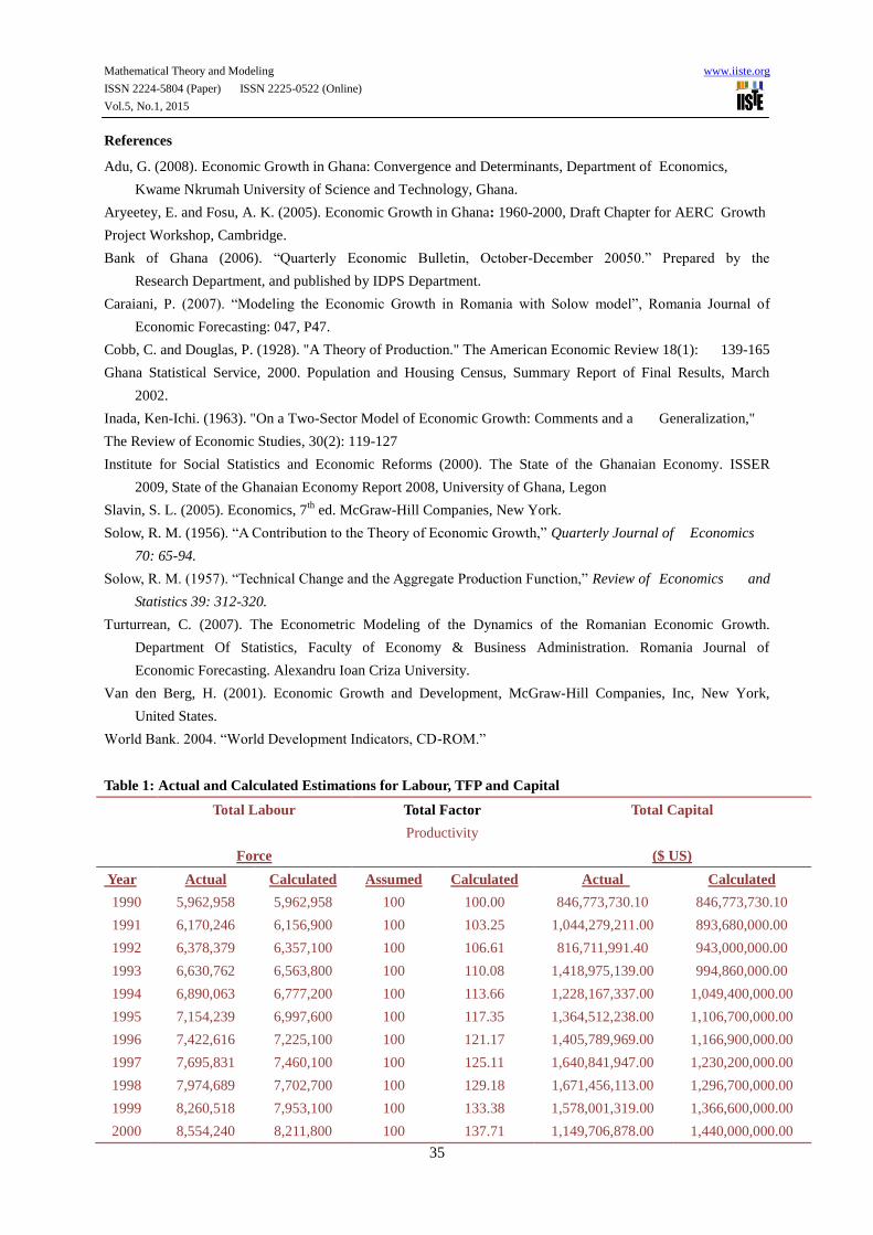
From Table 1, it can be observed that the actual data for labour over the periods 1990 to 2010 seem to be building

up over the period. But, the calculated figures of labour seemed to be growing faster than that of the actual labour

supply. The calculated figures for TFP seem to be growing over the period, indicating that in the long run when

growth rate of capital is constant, growth in GDP may be as a result of change in the level education, change of

technology, etc. This was not the case in Cobb-Douglas model, where TFP was assumed to be constant. Both actual

and calculated figures for capital were evenly spread from 1990 to 2003 and uneven from 2004 to 2010. This is a

reflection of real life situation. It should be understood that capital acquisition and usage could not be consistent as

it depends on the changing needs of the economy as it has pointed out earlier on by Baafi (2010). The calculated

figure for the capital over the period seemed to be building up with time.

The actual Production (GDP) figures were evenly spread over the period (See Table 2). They were higher in certain

periods and lower in other periods. The calculated figures for production consistently build up over the periods. It

increases year after year; highest in the last year under consideration, 2010 with a figure of 7,090,300,000.00.

Considering the production/GDP growth rate, the following findings were apparent. The growth rates were evenly

spread for most of the years under consideration, especially, 1997, 2001, and 2002 as shown in Table 3.

The actual average growth rate from 1984 to 2010 according to http://data.worldbank.org/country/ghana and

African Development indicator 2007 for Ghana was 4.5% which is relatively close to the calculated average

growth rate of 4.21%.

Figure 1 depicts the production/GDP for the economy, which builds up from year to year. The actual production

values were always above that of the calculated throughout the periods under consideration.

Figure 2 depicts the rate at which production builds up from year to year. From the graph it is apparent to see that

growth rates were positive throughout the period under consideration. It was also interesting to know that the

difference between the growth rates were marginal. The actual growth rates for some periods were always above

that of the calculated throughout the periods, except 1992, 1994, 2000 and 2009. The actual average growth rate

over the period was 4.5% as compared to the calculated value of 4.21%. From the graph the computed figures


http://data.worldbank.org/country/ghana



Vol.5, No.1, 2015

33

appear in red line. This is so because the variances between the rates were very small. This showed that the growth

rate of Ghana has been slow as was noted by Aryeetey and Fosu (2005).

The actual production per labour started from a high figure of $ 547.86 per labour in 1990 and kept increasing

throughout the period. The calculated production per labour started at $547.86 and reduced to $515.28 in 1991 and

started increasing from1993. The variances between the figures were very small from 1990 t0 2004 and afterwards

the actual figures started growing faster than the calculated (refer to Figure 3)

Observe from Figure 4 that the actual capital per labour was uneven over the periods under consideration. It

increases and decreases throughout the period. The figure ranges between $142.01 per labour in 1990 and $483.82

in 2010. The calculated capital per labour started with a figure of $145.15 in 1991 grew steadily over the period to

record $213.08 per labour in 2010.

As is depicted in figure 5, the actual percentage change was uneven over the periods. It ranges between a low

figure -27.14 percent in 2000 to as high a figure of 73.74 percent in 1993. There were fluctuations in the rate of

change of capital over the periods. The calculated change in capital ranges between 5.22 percent in 2010 and 5.54

percent in 1990. But generally the percentage change lies between 0 and 100% making the graph smooth out

around the horizontal axis.

It is amazing figure 6 showed similarities between actual and calculated rate of change in Labour Supply. The only

difference was that the calculated rates of change were always higher for the periods 2001 to 2010 and vice versa

for the periods before 2001. Though the changes were uneven, the two lines showed similar patterns. The actual

figure ranges between 1% and 5% whilst the calculated ranges between 2% and 5%. Also, we observed that the

correlation coefficient between the actual growth rates and calculated was 0.298, indicating that the two variables

are correlated, but the strength of correlation is weak as can be observed in Table 4.

5. Conclusion

The purpose of the research was to establish an appropriate economic growth model to be studied mathematically

to measure economic growth. The principal determinants of economy’s growth were the labour supply, the active

working population, Capital, thus the non-human elements that adds to labour for productivity and finally the level

of technological advancement in the economy. The conditions surrounding economy’s growth would be an

appropriate environment for both capital accumulation and healthy labour force coupled with the most appropriate

technology. The short-run relation results presented show that, there is a positive relation between the factors of

production and real GDP, both for actual and the calculated. Thus as elements used in production increases, we

expect the GDP also to increase. The results on total factor productivity show that, there is a positive relation

between real GDP growth and TFP. That is in the long run GDP growth may be as result of change in the level of

technology, level of education etc.

The long-run relation results show that, there is a positive relationship between real GDP growth and capital,

proxy by Gross domestic fixed capital formation. The results indicated that a percentage change in capital stock

lead to a 0.4 percentage change in real GDP growth. The long run relations results show a negative relation

between GDP and labour proxy by labour force. The results indicate that, real GDP growth falls by -1.2 percent

as labour force increases by one unit. Thus in the long run when GDP is constant or decreasing, a small increase

in labour supply will reduce the GDP growth rate. Comparing the outcome of our model to the actual data




Vol.5, No.1, 2015

34

gathered from the Ghana Statistical Service, World Bank Group and MOFEP. The results showed a very close

relationship between the actual (4.5%) and calculated (4.25%) average growth rate over the periods 1990 to

2010.

Economic growth is defined as the increase in the amount of goods and services produced by an economy over

time. Economy’s performance is generally measured using GDP (Gross Domestic Product) by Economists.

Being able to discern and measure progress more comprehensively that with GDP, is a key prerequisite for

improved decision making. The principal determinants of the economy’s growth as used in this study were

capital, labour and Total Factor productivity (T.F.P).

According to Slavin (2005), “growth is the quantitative increase in physical scale while development is qualitative

improvement or the unfolding of potentiality. An economy can grow without developing, or develop without

growing, or do both or neither”.

The determinants have the following effects on the growth of the economy; α and β are the output elasticities of

labour and capital respectively are constants determined by available technology. Output elasticity measures the

responsiveness of output to a change in levels of either labour or capital used in the production, ceteris paribus.

Cobb-Douglas model assumed that α= 0.7 and β= 0.3, which was one of the assumptions used in the models. For

example if: α= 0.2, a 1% increase in labour would lead to approximately a 0.2% increase in output. Further, if: α+

β= 1, the production function has a constant returns to scale. That is, if L and K are each increased by 20%, Y

increases by 20%. If: α+ β<1, returns to scale are decreasing, and if: α+ β> 1, returns to scale is increasing.

Assuming perfect competition, α and β can be shown to be labour capital’s share of output.

Solow simplify that an economy-wide production function as , as indicated in (8). Solow

assumed that TFP is proportional to itself, unlike Cobb-Douglas, which estimated TFP to be equal to 1 in their

function. Solow again argued that, since technology changes over time and increases in the level of education

also changes over time, it was prudent to allow TFP to also grow proportional to it. A little work needs to be

done on the parameters α, β from time to time in the production function. The appropriate model is the model

that answers all the questions of the system being described by the models. For example our production model of

the economy’s growth at (24), could be said to describe the system of economy’s growth if it computes the

intended output of the economy appropriately.

Finally, comparing the outcome of our model to the actual data we gathered from the Ghana Statistical Service,

World Bank Group and MOFEP. The results showed a very close relationship between the actual (4.5%) and

calculated (4.21%) average growth rate over the periods 1990 to 2010. This model predicted the growth pattern

very well and it is our thinking that a little work needs to be done on the parameters to put the results into

perspective. Therefore, Solow’s growth model predicts the growth pattern of Ghana’s economy.

Acknowledgements

Our salutations go to Dr. Osei-Frimpong of Mathematics Department, Kwame Nkrumah University of Science

and Technology, Kumasi, and Dr. Emmanuel Mensah Baah, Dean of the Academic Quality Assurance Unit,

Takoradi Polytechnic for their encouragement and support during the preparation of this paper. God bless you

Docs. Your backing was great.




Vol.5, No.1, 2015

35

References

Adu, G. (2008). Economic Growth in Ghana: Convergence and Determinants, Department of Economics,

Kwame Nkrumah University of Science and Technology, Ghana.

Aryeetey, E. and Fosu, A. K. (2005). Economic Growth in Ghana: 1960-2000, Draft Chapter for AERC Growth

Project Workshop, Cambridge.

Bank of Ghana (2006). “Quarterly Economic Bulletin, October-December 20050.” Prepared by the

Research Department, and published by IDPS Department.

Caraiani, P. (2007). “Modeling the Economic Growth in Romania with Solow model”, Romania Journal of

Economic Forecasting: 047, P47.

Cobb, C. and Douglas, P. (1928). "A Theory of Production." The American Economic Review 18(1): 139-165

Ghana Statistical Service, 2000. Population and Housing Census, Summary Report of Final Results, March

2002.

Inada, Ken-Ichi. (1963). "On a Two-Sector Model of Economic Growth: Comments and a Generalization,"

The Review of Economic Studies, 30(2): 119-127

Institute for Social Statistics and Economic Reforms (2000). The State of the Ghanaian Economy. ISSER

2009, State of the Ghanaian Economy Report 2008, University of Ghana, Legon

Slavin, S. L. (2005). Economics, 7th

ed. McGraw-Hill Companies, New York.

Solow, R. M. (1956). “A Contribution to the Theory of Economic Growth,” Quarterly Journal of Economics

70: 65-94.

Solow, R. M. (1957). “Technical Change and the Aggregate Production Function,” Review of Economics and

Statistics 39: 312-320.

Turturrean, C. (2007). The Econometric Modeling of the Dynamics of the Romanian Economic Growth.

Department Of Statistics, Faculty of Economy & Business Administration. Romania Journal of

Economic Forecasting. Alexandru Ioan Criza University.

Van den Berg, H. (2001). Economic Growth and Development, McGraw-Hill Companies, Inc, New York,

United States.

World Bank. 2004. “World Development Indicators, CD-ROM.”

Table 1: Actual and Calculated Estimations for Labour, TFP and Capital

Total Labour

Total Factor

Productivity

Total Capital

Force ($ US)

Year Actual Calculated Assumed Calculated Actual Calculated

1990 5,962,958 5,962,958 100 100.00 846,773,730.10 846,773,730.10

1991 6,170,246 6,156,900 100 103.25 1,044,279,211.00 893,680,000.00

1992 6,378,379 6,357,100 100 106.61 816,711,991.40 943,000,000.00

1993 6,630,762 6,563,800 100 110.08 1,418,975,139.00 994,860,000.00

1994 6,890,063 6,777,200 100 113.66 1,228,167,337.00 1,049,400,000.00

1995 7,154,239 6,997,600 100 117.35 1,364,512,238.00 1,106,700,000.00

1996 7,422,616 7,225,100 100 121.17 1,405,789,969.00 1,166,900,000.00

1997 7,695,831 7,460,100 100 125.11 1,640,841,947.00 1,230,200,000.00

1998 7,974,689 7,702,700 100 129.18 1,671,456,113.00 1,296,700,000.00

1999 8,260,518 7,953,100 100 133.38 1,578,001,319.00 1,366,600,000.00

2000 8,554,240 8,211,800 100 137.71 1,149,706,878.00 1,440,000,000.00


http://en.wikipedia.org/wiki/The_Review_of_Economic_Studies



Vol.5, No.1, 2015

36

2001 8,808,936 8,478,800 100 142.19 1,439,998,829.00 1,517,100,000.00

2002 9,068,519 8,754,500 100 146.81 1,156,455,431.00 1,598,100,000.00

2003 9,331,979 9,039,200 100 151.59 1,748,749,261.00 1,683,100,000.00

2004 9,585,053 9,333,100 100 156.52 2,517,616,120.00 1,772,400,000.00

2005 9,852,131 9,636,600 100 161.61 3,109,129,779.00 1,866,200,000.00

2006 10,120,320 9,949,900 100 166.86 4,411,164,569.00 1,964,600,000.00

2007 10,376,027 10,273,000 100 172.29 4,953,021,277.00 2,067,900,000.00

2008 10,647,454 10,608,000 100 177.89 6,119,680,499.00 2,176,400,000.00

2009 10,925,982 10,952,000 100 183.68 5,122,231,687.00 2,290,200,000.00

2010 11,211,796 11,309,000 100 189.65 5,424,443,356.53 2,409,700,000.00

Source: Result from analysis of data

Table 2: Actual and Calculated Estimations for GDP and GDP Growth Rate

(Production) (Production)

GDP (constant 2000 US$) GDP Growth Rate Periods

Year Actual Calculated Actual Calculated (t)

1990 3,266,886,838.00 3,266,886,838.00 3.33 3.33 0

1991 3,439,438,121.00 3,172,500,000.00 5.28 2.89 1

1992 3,572,868,343.00 3,303,200,000.00 3.88 4.12 2

1993 3,746,152,457.00 3,440,100,000.00 4.85 4.14 3

1994 3,869,775,489.00 3,583,500,000.00 3.27 4.17 4

1995 4,028,916,869.00 3,733,600,000.00 4.02 4.19 5

1996 4,214,346,194.00 3,890,900,000.00 4.6 4.21 6

1997 4,391,195,243.00 4,055,600,000.00 4.2 4.23 7

1998 4,597,598,580.00 4,228,200,000.00 4.57 4.26 8

1999 4,799,892,758.00 4,409,200,000.00 4.55 4.28 9

2000 4,977,488,790.00 4,598,800,000.00 3.74 4.3 10

2001 5,176,588,342.00 4,797,700,000.00 4.18 4.33 11

2002 5,409,534,817.00 5,006,200,000.00 4.46 4.35 12

2003 5,690,830,628.00 5,224,900,000.00 5.34 4.37 13

2004 6,009,517,143.00 5,454,300,000.00 5.58 4.39 14

2005 6,364,078,886.00 5,695,000,000.00 5.86 4.41 15

2006 6,771,379,934.00 5,947,600,000.00 6.43 4.44 16

2007 7,208,793,173.00 6,212,800,000.00 5.7 4.46 17

2008 7,816,530,776.00 6,491,100,000.00 7.23 4.48 18

2009 8,180,601,366.00 6,783,400,000.00 4.14 4.5 19

2010 8,664,892,967.00 7,090,300,000.00 5.92 4.52 20





Vol.5, No.1, 2015

37

Table 3: Actual and Calculated Estimations GDP/Production per labour, Capital per Labour, Rate of

Change of Capital and Rate of change of labour.

GDP/Production per

labour

Capital per Labour Rate of Change of

Capital

Rate of Change of Labour

Year ($ US) ($ US) (%) (%)

Actual Calculated Actual Calculated Actual Calculated Actual Calculated

1990 547.86 547.86 142.01 142.01 - - - -

1991 557.42 515.28 169.24 145.15 23.32 5.54 3.48 3.25

1992 560.15 519.61 128.04 148.34 -21.79 5.52 3.37 3.25

1993 564.97 524.10 214.00 151.57 73.74 5.50 3.96 3.25

1994 561.65 528.76 178.25 154.84 -13.45 5.48 3.91 3.25

1995 563.15 533.55 190.73 158.15 11.10 5.46 3.83 3.25

1996 567.77 538.53 189.39 161.51 3.03 5.44 3.75 3.25

1997 570.59 543.64 213.21 164.90 16.72 5.42 3.68 3.25

1998 576.52 548.92 209.60 168.34 1.87 5.41 3.62 3.25

1999 581.06 554.40 191.03 171.83 -5.59 5.39 3.58 3.25

2000 581.87 560.02 134.40 175.36 -27.14 5.37 3.56 3.25

2001 587.65 565.85 163.47 178.93 25.25 5.35 2.98 3.25

2002 596.52 571.84 127.52 182.55 -19.69 5.34 2.95 3.25

2003 609.82 578.03 187.39 186.20 51.22 5.32 2.91 3.25

2004 626.97 584.40 262.66 189.90 43.97 5.31 2.71 3.25

2005 645.96 590.98 315.58 193.66 23.49 5.29 2.79 3.25

2006 669.09 597.75 435.87 197.45 41.88 5.27 2.72 3.25

2007 694.75 604.77 477.35 201.29 12.28 5.26 2.53 3.25

2008 734.12 611.91 574.76 205.17 23.55 5.25 2.62 3.26

2009 748.73 619.38 468.81 209.11 -16.30 5.23 2.62 3.24

2010 772.84 626.96 483.82 213.08 5.90 5.22 2.62 3.26


Table 4: Correlation coefficients

Calculated value

from the model

Actual values from MOFEP,

World Bank Group

Calculated value from the

model

Pearson Correlation 1 0.298

Sig. (2-tailed) 0.189

N 21 21

Actual values from

MOFEP, World Bank

Group

Pearson Correlation 0.298 1

Sig. (2-tailed) 0.189

N 21 21





Vol.5, No.1, 2015

38

Figure 1: Production/GDP (constant 2000 US$

Figure 2: Production/GDP Growth Rate

Figure 3: Production per Labour




Vol.5, No.1, 2015

39

Figure 4: Capital per Labour

Figure 5: Percentage change in Capital

Figure 6: Rate of change of Labour Supply


The IISTE is a pioneer in the Open-Access hosting service and academic event management.

The aim of the firm is Accelerating Global Knowledge Sharing.

More information about the firm can be found on the homepage:

http://www.iiste.org

CALL FOR JOURNAL PAPERS

There are more than 30 peer-reviewed academic journals hosted under the hosting platform.

Prospective authors of journals can find the submission instruction on the following

page: http://www.iiste.org/journals/ All the journals articles are available online to the

readers all over the world without financial, legal, or technical barriers other than those

inseparable from gaining access to the internet itself. Paper version of the journals is also

available upon request of readers and authors.

MORE RESOURCES

Book publication information: http://www.iiste.org/book/

Academic conference: http://www.iiste.org/conference/upcoming-conferences-call-for-paper/

IISTE Knowledge Sharing Partners

EBSCO, Index Copernicus, Ulrich's Periodicals Directory, JournalTOCS, PKP Open

Archives Harvester, Bielefeld Academic Search Engine, Elektronische Zeitschriftenbibliothek

EZB, Open J-Gate, OCLC WorldCat, Universe Digtial Library , NewJour, Google Scholar


http://www.iiste.org/journals/

http://www.iiste.org/book/

http://www.iiste.org/conference/upcoming-conferences-call-for-paper/

modelling the economic growth rate of ghana using the

Documents