Modelling the age-dependent personal income distribution in the USA Ivan O. Kitov

IDG RAS

VIC P.O. Box 1250

Vienna, A-1220 Austria

ikitov@mail.ru Abstract Numerical modelling of the age-dependent personal income distribution (PID) in the USA is fulfilled based on a micro- and macroeconomic model and results of the overall PID modelling. The model has demonstrated an excellent prediction power in almost all income bins except the lowermost ones.

Here we address the problem of the fine age structure of the PIDs. The age-dependent PIDs are modelled by using the same defining parameters as the overall PIDs. The predicted PIDs accurately describe the observed ones reproducing such complex features as the exponential PID decay in the youngest and oldest age groups. The evolution of the age-dependent PIDs in time is also accurately predicted. The difference in the PID levels in the youngest age group is explained by some shortcomings in the design of the enumeration procedure. Corresponding recommendations are given in order to improve the PID estimates. Key words: personal income distribution, mean income, microeconomic modeling, USA, real GDP, macroeconomics JEL Classification: D01, D31, E17, J1, O12

1

Modelling the age-dependent personal income distribution in the USA Ivan O. Kitov

Abstract Numerical modelling of the age-dependent personal income distribution (PID) in the USA is fulfilled based on a micro- and macroeconomic model and results of the overall PID modelling. The model has demonstrated an excellent prediction power in almost all income bins except the lowermost ones.

Here we address the problem of the fine age structure of the PIDs. The age-dependent PIDs are modelled by using the same defining parameters as the overall PIDs. The predicted PIDs accurately describe the observed ones reproducing such complex features as the exponential PID decay in the youngest and oldest age groups. The evolution of the age-dependent PIDs in time is also accurately predicted. The difference in the PID levels in the youngest age group is explained by some shortcomings in the design of the enumeration procedure. Corresponding recommendations are given in order to improve the PID estimates.

Introduction Numerical modelling of the age-dependent personal income distribution (PID) in the USA is

fulfilled based on a micro- and macroeconomic model and results of the overall PID modelling.

Kitov (2005a) formally introduced a microeconomic model for a personal income evolution as a

function of individual capacity to earn money and economic growth. The sum of all the personal

incomes predicted by the microeconomic model (with a simple assumption about the distribution

of the capacity to earn money) builds a macroeconomic model. Defining parameters of the

macroeconomic model providing the best fit between the observed and predicted PIDs are

presented and briefly discussed in the paper.

Kitov (2005b) presented results of the overall PID modelling. Principal features of the

observed PIDs’ are revealed and discussed. The uncovered characteristics provide a deterministic

description of the PID shape and its evolution in time. As a result, the macroeconomic model

accurately describes the observed evolution of the overall PID between 1994 and 2002. The two

papers present a concept of two branches of the PIDs: a lower income branch and a high income

branch. The former is accurately described by the model and the latter is a standard Pareto

distribution. The Pareto distribution (or power law distribution) results from a number of

processes called as a whole “self-organized criticality”. There is no economic model available to

formally express the processes leading to the observed Pareto distribution and only the number

of people governed by this distribution is predicted by the developed macroeconomic model. The

number of people is the only parameter needed to model the observed Pareto distribution because

other parameters of the distribution are fixed for a given society.

2

The overall PIDs presented in (Kitov 2005b) include the personal incomes of all the

Americans above 15 years of age as published by the U.S. Census Bureau (2004a). By design,

aggregation in narrow income bins of $2500 does not depend on age. It is obvious, however, that

each and every personal income undergoes important changes with time. The starting point for

any personal income is apparently a zero income. Then the income grows with decreasing rate

to some maximum value. Between 1994 and 2002, the observed personal incomes in the USA

usually reached their relative maximum value at some age between 45 and 55 years and then

dropped. The overall PIDs are not able to describe all these complex features and processes due

to lack of age resolution. The processes and features, however, are extremely important from a

personal point of view as a prospective of income trajectory. They are also a big challenge to any

model for the personal income distribution and its evolution. In Section 1 of this paper, we

briefly discuss some problems related to the PID and its evolution in various age groups. The

high resolution data set under analysis is obtained from the same source as in the previous papers

– the U.S. Census Bureau (2004). In Section 2, we consistently apply the microeconomic and

macroeconomic model to accurately predict the observed behaviour of the age-dependent PIDs.

Some principal results of the modelling are presented in graphic form. Conclusions made in

Section 3 are discussed in a broader economic context.

1. Evolution of the personal income distribution in various age groups: Observations

The overall PIDs in the USA studied and modelled by Kitov (2005b) demonstrate a very stable

structure of the society in respect to distribution of the total income. However, the observed PIDs

change very fast from one age group to another. The personal income data sets with high age

resolution for years between 1994 and 2002 include information on the number of people in 5

year wide age intervals starting with 15 years of age. The first interval is twice as long, however,

and spans the age interval between 15 and 24 years. This widening reflects enumeration

problems in this age group, where standard definitions of income (as listed in the technical paper

63RV of the US Census Bureau (2002b)) do not cover all potential income sources as, for

example, interfamily money transfer.

Figures 1 and 2 display the PIDs measured in 1998 in various age groups in absolute

values and normalized to the total population above 15 years of age respectively. In the youngest

age group, the distribution is close to an exponential one with strong variations observed at

3

incomes above $50K. This is a result of the Current Population Survey (CPS) and Annual Social

and Economic Supplement (ASEC) to the CPS procedures covering only approximately 100,000

households (The US Census Bureau 2002a). When the PID in this relatively narrow age group

drops by three orders of magnitude, this coverage can not provide adequate estimates. At higher

income, there are no counted people at all. It is expressed by gaps in the distribution curves or

zero values in corresponding tables. Thus, one should always keep in mind that the high income

tail of the age-dependent PIDs are not reliable and the strong variations have an artificial

character representing no actual distribution. (These artificial gaps are also partly responsible for

the underestimated average income in the youngest age group as will be discussed in the next

paper.)

With increasing age or work experience (equal to the actual age of a person minus the

work starting age of 15 years), the PIDs obtain a slowly extending quasi-flat part and a quasi-

exponential decreasing part. The PID for the age group between 70 and 74 years is characterized

as a whole by an exponential roll-off similar to that for the youngest group. This indicates that

old people in the USA lose income very fast with time and not many of them can retain the same

income as they had before: compare the oldest group with the group between 60 and 64 years of

age. Figure 2 illustrates this process in relative units. The curve corresponding to the oldest

reported age group lies below the curve for the age group between 25 and 29 years for incomes

higher than $30K and well above this curve for incomes below $20K. The middle age groups are

characterized by very closely bunched population density-income distributions. Thus, the

observed PIDs for a single calendar year (1998) uncover a complex character of their evolution

with age. The PIDs for other years of the studied interval are similar and show the same principal

features.

Of the same principal importance is the evolution of the PIDs with time observed in the

same age groups. Figure 3 shows two PIDs (current dollars) in the youngest age group for

calendar years 1994 and 2002. An exponential regression gives a negative index, increasing from

-0.125 in 1994 to -0.095 in 2002. The ratio of the indices is 1.32. This value is very close to that

observed for per capita nominal GDP growth from 1994 to 2002, equal to 1.34 (Bureau of

Economic Analysis 2005). Thus, an adjustment for the per capita nominal GDP growth like the

one applied to the overall distribution by Kitov (2005b) would completely merge the curves.

4

Figures 4 and 5 show results of an exponential regression analysis of the second (or

decreasing) PID part (the quasi-flat parts are not shown) for the age groups from 24 to 29 years

and from 45 to 49 years. Figure 6 summarizes results of the exponential regression study

depicting the indices obtained for calendar years 1994 and 2002 in various age groups. The index

curves decrease with age according to a power law. Both calendar years are characterized by the

same exponent of -0.5. Thus, one can assume that the ratio of indices for all the ages is the same

and equal to 1.33, i.e. the ratio of the power law coefficients, 0.2864/0.2011=1.33, and that all

the PIDs return to that for 1994 if corrected for the per capita nominal GDP growth. This

assumption may be not so accurate, however, for the age groups around 50 years.

There are four principal features of the original PIDs dependence on work experience we

would like to stress. The first is the exponential character of the distribution in the youngest age

group over the whole reported income range. The second is the development of the quasi-

constant part of the normalized distributions extending from a zero income to approximately

$30K in the age groups above 25 years. The third important phenomenon is a fast decrease of the

distribution for the oldest age group. The distribution in this group shows a character similar to

the distribution in the youngest age group. One can assume that in some older age group, above

75 years of age, the distribution is the same as in the youngest group. And the fourth observation

is the synchronized development of the quasi-exponential roll-off parts of the distributions over

the years. Despite the change of the exponential indices with work experience, their ratio is

almost the same for the 1994 and 2002 PIDs.

The adjustment for the per capita nominal GDP growth effectively returns the overall

PID to the original one, as shown by Kitov (2005b). The same procedure is applied to the PIDs

in the studied age groups. Some results of the data processing are presented in Figures 7 through

9. In the youngest age group, the adjustment results in the same pattern as observed for the

overall distribution. The only difference is a higher scattering at higher incomes related to the

lack of reliable data in this income range, as discussed above. The largest differences between

the adjusted PID are observed for the age groups from 45 to 49 years and from 50 to 54 years

(Figures 8 and 9, respectively). These groups are near the age where the mean personal income

distribution over work experience changes from growth to fall. This critical age also changes

with time as the square root of the per capita real GDP growth (Kitov 2005a). So, one can expect

5

the largest disturbance in the PID near this age, which is currently between 50 and 55 years of

age in the USA.

2. Modelling personal income distribution in various age groups

The personal income distributions in the age groups published by the U.S. Census Bureau are

calculated in the course of the overall prediction by using the macroeconomic model developed

by Kitov (2005a). Since the model calculates each and every individual income, it is a very

simple procedure to calculate the number of people in any given age and/or income interval.

Actually, the model takes into account only 841 distinct individual income histories for every

single year of age, but corrects for the total number of people having the same age. Thus, people

of the same age are effectively divided into 841 equal groups, and size of these groups changes

with age.

Briefly the model presented by Kitov (2005a) is as follows. A personal income depends

on two principal parameters. The first one is the economic growth expressed in per capita (real or

nominal) GDP growth rate. The second parameter is a product of the personal capability to earn

money and the size of earning means. Having these parameters, one can predict any personal

income trajectory by using relationships (2) and (3) from (Kitov 2005a). Each trajectory has two

branches: increasing and decreasing. The former is described by a function of type (1-exp(-αt)),

where α is a small parameter dependent on the personal size of earning means, and t is the

personal work experience. The second branch is exactly described by a function exp(-α1t), where

α1 is also a small parameter, which in general case is not equal to α. The increasing branch

transits into the decreasing one at some critical work experience Tcr. The value of Tcr evolves in

time as the square root of the per capita real GDP. In 2002, the Tcr was of about 40 years in the

USA.

In absolute terms, both factors of the product representing the capacity to earn money

grow proportionally to the square root of the observed per capita (real or nominal depending on

whether the data presented in real or nominal dollars) GDP making the product to be

proportional to the per capita GDP growth itself. This growth of the absolute value of the

personal income with calendar year corresponds to a drift coordinated with the overall evolution

of the economy. Thus, each and every personal income is assumed to be growing proportionally

to the observed GDP growth rate. At the same time, each personal income evolves relative to

6

other personal incomes as the person gets older. (One can consider two time scales: a global time

scale for the economy as a whole – calendar years; and a local scale for the person – age). In the

beginning, this relative growth is fast and then it is slowing down to reach a zero growth rate at

Tcr. If there is no economic growth in the country (Tcr is constant), the pattern of the relative

growth will repeat itself: the personal income trajectories are all the same and do not depend on

the starting year of work. Any economic growth, whether positive or negative, leads to the

change of the size of earning means and Tcr as well. The change distorts the personal income

trajectories and the overall pattern of the relative personal incomes’ growth.

For people of the same age (for the sake of simplicity we assume that all the people of the

same age have the same birthday and start day of work), there are only 841 possible personal

income trajectories. These trajectories correspond to 841 distinct combinations of the individual

capability to earn money and the size of earning means available according to the even

distribution of these two factors as integer numbers between 2 and 30 (841=29x29).

Everybody can choose one of the trajectories and follow it in time. The person can also

jump from one trajectory to another. The latter forces somebody who had before the new

trajectory of the first person to drop to the left trajectory, i.e. the trajectories can be only swapped

not created. Thus, the relative distribution of the personal incomes is the same for people of the

same age. Ratio of personal incomes of two persons with the same capacity to earn money and

the same size of earning means but of different age depends on the observed economic growth

during the period between the calendar years they started their job careers.

The model’s defining parameters Tcr and α depend on time in a developing economy

(Kitov 2005a). A series of calculations has been conducted for various time intervals between

1950 and 2002 in order to obtain the best estimates of the defining parameters (Kitov 2005b).

The best fit parameters for 1960 (the start year of the age dependent PID study) are Tcr=26.5

years and α=0.087, respectively. These values can be reduced to any year other than 1960 by

using the per capita real GDP growth rate.

Figures 10 through 13 show the observed and predicted distributions in the age groups

from 15 to 24 years, from 25 to 29 years, from 30 to 34 years, and from 60 to 64 years in 1998.

This year has an advantage of a very simple conversion factor between the model dimensionless

units and the observed currency units (dollars) equal to 10,000. This means that 1.0 model unit

costs $10,000 in 1998 and scaling of the model results to those observed is straightforward. As

7

has been already shown, the other middle age groups have distributions very similar to those for

the age groups from 30 to 34 years and from 60 to 64 years.

In the youngest age group, the distributions diverge almost everywhere. The predicted

distribution lies above the actual one. One can explain this observation by the factors discussed

above: the low resolution in this group, the undercounting at higher incomes and the absence of

adequate income sources in the Census Bureau’s questionnaire. So, this deviation is expectable

and should be resolved somehow in further income surveys, i.e. this deviation is induced by

some deficiencies in the current design and methodology of the surveys not by the model. Both

distributions are characterized, however, by the same indices of the exponential decay from the

zero income bin to the income bin starting at $40K. The observed distribution has already an

emergent part characterized by the Pareto distribution (above $48K) and also has a large number

of people with very low income. The latter observation is consistent with the predicted

behaviour. Again, the accuracy of the enumeration at lower incomes is under doubt due to the

limited questionnaire.

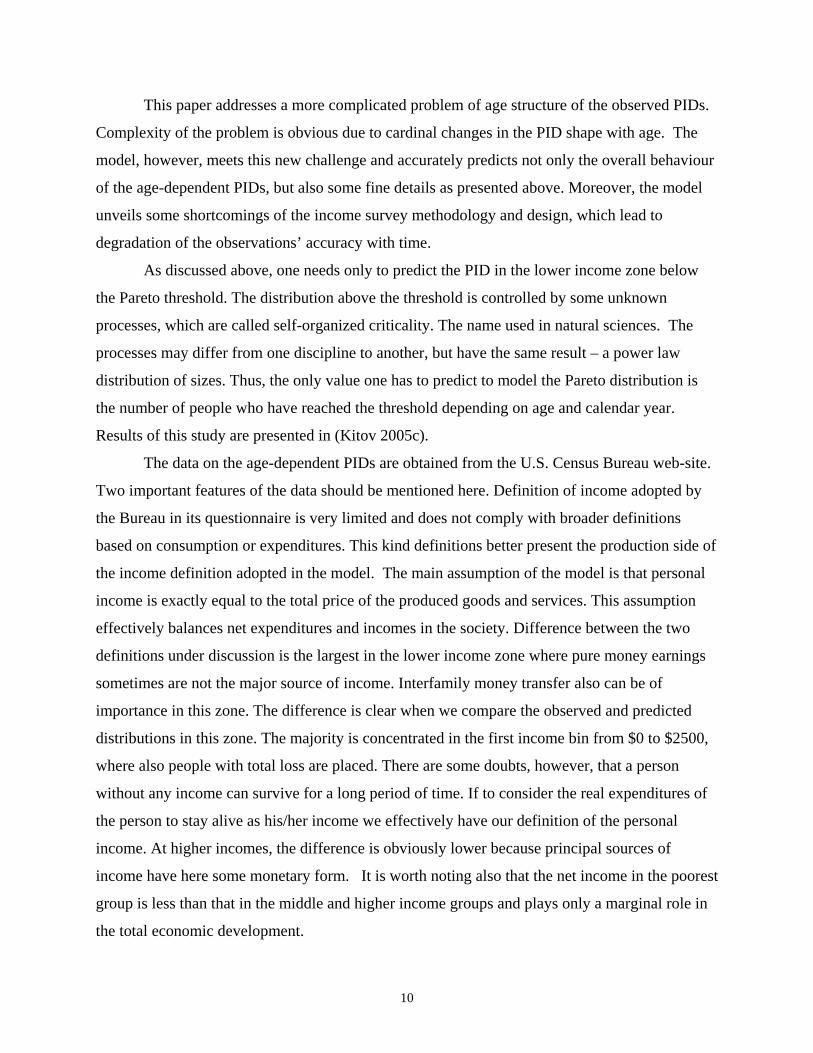
In the middle age groups, evolution of the predicted and observed distribution is

described with reasonable accuracy. Here we meet again the low income counting problem. In

the oldest age group among the ones presented here (from 60 to 64 years of age), the theoretical

curve fits the measured one with an excellent precision. As in the overall PID (Kitov 2005b), one

can distinguish a sub-critical zone, a zone where the theoretical distribution is above the

observed and a zone of an opposite behaviour. The same age group has been used for calibration

of the earning capabilities (Kitov 2005a).

The actual PIDs lack resolution in the most important age group – from 15 to 24 years of

age where dynamics of the income evolution is the fastest. The observed PID for this age interval

actually consists of ten very different single year PIDs. Figure 14 displays the predicted

evolution of the single year of age PIDs for 1998 starting from 3 years of work experience, i.e.

decomposition of the aggregated distribution into the single year of age distributions. During the

first two years of work the predicted incomes are concentrated in the lowermost income bins.

The predicted evolution reveals some important features of the PIDs. During the first eight years

of work nobody was able to reach the Pareto distribution income range starting from $48K (the

Pareto distribution threshold). This can be the actual reason for the U.S. Census Bureau to

aggregate all the personal incomes between 15 years and 24 years of age. Otherwise, there is

8

almost nobody filling the high income bins in the Pareto distribution range. (There are actually

quite a few people starting their job career before reaching the age of 15 years. There is no

official statistics for these people, however, and their overall impact is negligible in the course of

the PID evolution because they affect only the youngest age group with the lowermost incomes.

With age, all these differences in the start year of work are smoothed.)

In addition to a higher age resolution, the predicted PID can be extrapolated years back

and ahead. Figure 15 and 16 compare the predicted PID in 5 year wide work experience intervals

for calendar years 1980 and 2002. One can observe that the PIDs span very different ranges of

income despite the same virtual procedure of counting in $2500 wide intervals. In 1980, the

predicted distributions lie inside the income interval from $0 to $35K. The Pareto distribution

threshold was of about $20K according to the nominal per capita GDP increase by 2.9 times

from 1980 to 2002. (An actual distribution, if measured, would be characterized by the Pareto

law above $20K and would be extended to very high incomes well above the model predicted

$35K.) In 2002, the Pareto threshold was of about $58K and the predicted distributions occupy

the whole income range of the actual survey – from $0 to $100K. One of the effects of the

observed PID stretching with time is that relatively lower number of people occur in the

predefined income intervals. This effect results in the observed oscillations in the PIDs. The

PIDs in 1980 look much smoother than in 2002 due to smoothing effects of the large numbers.

Oscillations in the predicted PID are only induced by the discrete distribution of the capacity to

earn money, which was revealed by the calibration procedure described by Kitov (2005a).

3. Discussion and conclusions

The personal income distribution in the USA was modelled for the period between 1994 and

2002 in the second paper of the series (Kitov 2005b) and found an excellent match between the

predicted and measured PIDs. This fact allowed us to assume that the model is adequate and to

calibrate the model as well. Defining parameters of the model obtained and described in the first

two papers occurred to be accurate in prediction of the PIDs’ evolution in time. The prediction of

the evolution was almost solely based on the assumption that the critical time, Tcr, and α evolve

as the square root of the per capita real GDP.

9

This paper addresses a more complicated problem of age structure of the observed PIDs.

Complexity of the problem is obvious due to cardinal changes in the PID shape with age. The

model, however, meets this new challenge and accurately predicts not only the overall behaviour

of the age-dependent PIDs, but also some fine details as presented above. Moreover, the model

unveils some shortcomings of the income survey methodology and design, which lead to

degradation of the observations’ accuracy with time.

As discussed above, one needs only to predict the PID in the lower income zone below

the Pareto threshold. The distribution above the threshold is controlled by some unknown

processes, which are called self-organized criticality. The name used in natural sciences. The

processes may differ from one discipline to another, but have the same result – a power law

distribution of sizes. Thus, the only value one has to predict to model the Pareto distribution is

the number of people who have reached the threshold depending on age and calendar year.

Results of this study are presented in (Kitov 2005c).

The data on the age-dependent PIDs are obtained from the U.S. Census Bureau web-site.

Two important features of the data should be mentioned here. Definition of income adopted by

the Bureau in its questionnaire is very limited and does not comply with broader definitions

based on consumption or expenditures. This kind definitions better present the production side of

the income definition adopted in the model. The main assumption of the model is that personal

income is exactly equal to the total price of the produced goods and services. This assumption

effectively balances net expenditures and incomes in the society. Difference between the two

definitions under discussion is the largest in the lower income zone where pure money earnings

sometimes are not the major source of income. Interfamily money transfer also can be of

importance in this zone. The difference is clear when we compare the observed and predicted

distributions in this zone. The majority is concentrated in the first income bin from $0 to $2500,

where also people with total loss are placed. There are some doubts, however, that a person

without any income can survive for a long period of time. If to consider the real expenditures of

the person to stay alive as his/her income we effectively have our definition of the personal

income. At higher incomes, the difference is obviously lower because principal sources of

income have here some monetary form. It is worth noting also that the net income in the poorest

group is less than that in the middle and higher income groups and plays only a marginal role in

the total economic development.

10

The second feature of the data is related to the coverage of the age and income intervals.

With the PIDs stretching with time over wider and wider income range, smaller and smaller

number of people are counted in the designed income bins. In the youngest age group, the

number of people changes by almost four orders of magnitude, i.e. if there are 10,000 people in

the lowermost income interval, less than ten people are present in the highest measured income

bin (See Fig. 1). In some income bins there is nobody counted in. This observation does not

present the real personal income distribution, but reveals only increasing problems in the current

survey design. There are two ways out: not to publish the data characterized by very high

uncertainty or to increase the population coverage (number of households) to make the data

accurate and representative.

The presented model is a good basis for the development of a new methodology for the

income distribution measurements and definitions of economic equality/inequality. Current

inequality measures like Gini coefficient and Lorenz curve usually say next to nothing about the

causes (driving forces) of the observed income distribution, are of artificial character, and are age

independent as well. The model predicts the evolution of the PID with economic growth and

reveals important future changes. For example, the overall economic growth results in longer

time necessary to reach higher income. This makes young people relatively poorer - a trend

which is observed in the USA. Further increase of Tcr and decrease of α will accelerate this

process in near future. Also, people reach the peak personal income later in age, but before the

retirement age: the former approaching the latter with the overall economic growth.

Acknowledgements

The author is grateful to Dr. Wayne Richardson for his constant interest in this study, help and

assistance, and fruitful discussions. The manuscript was greatly improved by his critical review.

11

References Bureau of Economic Analysis, U.S. Department of Commerce (2005) Table “Current-Dollar and "Real" Gross Domestic Product, (Seasonally adjusted annual rates)”, last modified 05.25.05, http://bea.gov/bea/dn/gdplev.xls Kitov, I.O. (2005a), “A model for microeconomic and macroeconomic development”, (in preparation) Kitov, I. O. (2005b) “Modelling the overall personal income distribution in the USA from 1994 to 2002" (in preparation) Kitov, I.O. (2005c) “Evolution of the personal income distribution in the USA: High incomes”, paper accepted for presentation at the first meeting of the Society for the Study of Economic Inequality (ECINEQ), Palma de Mallorca, July 20-22, 2005 U.S. Census Bureau (2002a) “Source and Accuracy of the Data for the March 2002 CPS” http://www.bls.census.gov/cps/ads/2002/S&A_02.pdf U.S. Census Bureau (2002b) “Technical Paper 63RV: Current Population Survey - Design and Methodology, issued March 2002”, http://www.census.gov/prod/2002pubs/tp63rv.pdf U.S. Census Bureau (2004a) "Detailed Income Tabulations from the CPS". Last Revised: August 26 2004; http://www.census.gov/hhes/income/dinctabs.html

12

Figures

Fig. 1. Personal income distribution in age groups. In the first age group (5) - from 0 to 9 years of work experience, an almost exponential decrease in observed.

13

Fig. 2. Population density vs. personal income in age groups from 15 to 24 years (5 – central point of corresponding work experience interval from 0 to 9 years), from 25 to 29 years (12.5), …, from 70 to 74 years (57.5). In the first age group an almost exponential decrease in observed.

14

Fig. 3. Population density vs. personal income in the age group from 15 to 24 years. The index of exponential regression function increases with time from -0.125 to -0.095.

15

Fig. 4. Exponential decrease of population density function with increasing personal income in the age group from 25 to 29 years. Flat portion of the distribution is skipped. The index of the exponential regression function increases with time from -0.0783 to -0.0585.

16

Fig. 5. Exponential decrease of population density function with increasing personal income in the age group from 45 to 49 years. The flat portion of the distribution is skipped. The index of the exponential regression function increases with time from -0.049 to -0.037.

17

Fig. 6. Index of the exponential regression function vs. work experience for years of 1994 and 2002. The power law regression of the indexes gives an exponent near -0.5 in both cases. The ratio of 1994 and 2002 indexes is 1.33.

18

Fig.7. Population density distribution in the age group from 15 to 24 years adjusted for the per capita nominal GDP growth. A strong scattering at higher incomes is induced by lack or resolution power of the current ASEC due to undercoverage of the population. Population density drops by three orders of magnitude with income increase from $5,000 to $45,000.

19

Fig.8. Population density distribution in the age group from 45 to 49 years adjusted for the per capita nominal GDP growth.

20

Fig.9. Population density distribution in the age group from 50 to 54 years adjusted for the per capita nominal GDP growth.

21

Fig. 10. Comparison of predicted and actual personal income distributions in the age group from 15 to 24 years. The actual distribution is characterized by an emergent Pareto part and lies almost everywhere below the predicted curve. The difference is associated with a poor procedure of the income survey which does not take into account money redistribution.

22

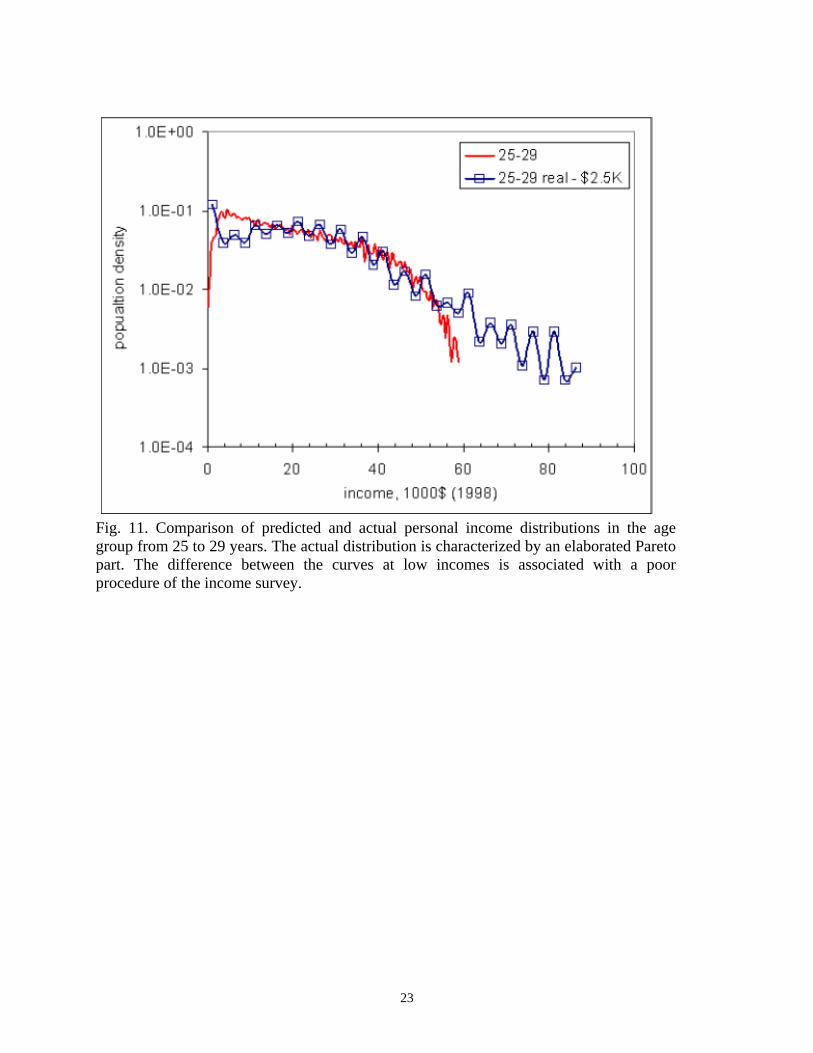
Fig. 11. Comparison of predicted and actual personal income distributions in the age group from 25 to 29 years. The actual distribution is characterized by an elaborated Pareto part. The difference between the curves at low incomes is associated with a poor procedure of the income survey.

23

Fig. 12. Comparison of predicted and actual personal income distributions in the age group from 30 to 34 years. The difference between the curves at low incomes is associated with poor procedure of the income survey.

24

Fig. 13. Comparison of predicted and actual personal income distributions in the age group from 60 to 64 years.

25

1

10

100

1000

0 10 20 30 40 50 6

income, $1K

#

0

345678910

Fig. 14. Evolution of the predicted personal income distribution (absolute number of people) in single year of age intervals between 3 years and 10 years of work experience.

26

1

10

100

1000

10000

0 5 10 15 20 25 30 35 40 45 50

income, $1K

#

15-2425-2930-3435-3940-4445-4950-5455-5960-6465-6970-74

Fig. 15 Evolution of the predicted personal income distribution (absolute number of people) in 1980.

27

1

10

100

1000

10000

0 20 40 60 80 100 120

income, $1K

#

15-2425-2930-3435-3940-4445-4950-5455-5960-6465-6970-74

Fig. 16 Evolution of the predicted personal income distribution (absolute number of people) in 2002.

28