optimal portfolio choice with path dependent labor income ...€¦ · optimal portfolio choice with...

Optimal portfolio choice with path dependentlabor income: the infinite horizon case

Fausto Gozzi

joint work with Enrico Biffis and Cecilia Prosdocimi

Milano, April 20, 2017

MotivationBenchmark model without path dependency

Sticky wages

Outline

1 Motivation

2 Benchmark model without path dependency

3 Sticky wages

Fausto Gozzi Optimal portfolio choice with path dependent labor income: the infinite horizon case


Sticky wages

Asset allocation

Merton (1971): wealth of the investor is given by risky andnon risky assets. Optimal for agents to put a constant fractionof their wealth in the risky asset throughout all their life

Starting from the ’90: models which add labor income to thewealth, see e.g. Bodie et al. (’92), Campbell-Viceira (’02),Fahri-Panageas (’07) Dybvig-Liu (’10). The total wealth of anagent is given by her financial wealth and her human capital,i.e. the present value of future labor income. Investors putoptimally a constant fraction of their financial wealth in therisky asset.

Empirical evidence of sticky wages: they respond to shocks inthe market, but with a delay (see Meghir-Pistaferri 2004)



Sticky wages

Our Goal.

Study a model of asset allocation where the wages arepath-dependent to describe more precisely their real behavior.First step of a project in progress.



Sticky wages

Outline

1 Motivation


3 Sticky wages



Sticky wages

The model of Dybvig, P.H. and Liu, H. (2010)

The market is Black & Scholes type:

dS0(t) =rS0(t)dt

dS1(t) =S1(t)µdt + S1(t)σdZ (t),



Sticky wages

dW (t) =[W (t)r + θ(t)(µ− r)− c(t) + δ

(W (t)− B(t)

)]dt

+ (1− R(t))y(t)dt + θ(t)σdZ (t), W (0) = W0

dy(t) =y(t)(µydt + σydZ (t)

), y(0) = y0

W (t) the wealth process, state

y(t) the labor income, state

θ(t) the dollar investment in the risky asset, control

c(t) the consumption, control

B(t) the bequest, control

R(t) := IT≤t and T is the retirement time, control

δ constant rate of mortality



Sticky wages

The death time τδ is modeled as a Poisson arrival time, withhazard rate δ.τδ is independent of the Wiener process (Z (t)).

We should consider as basic filtration the one generated byFτδ ∨ FZ , but we will actually work on τδ > t.

B(t) is the bequest-target we want to leave to the recipient:

for W (t)− B(t) < 0 we have to finance it buyingcontinuously a life insurance with premium δ(B(t)−W (t))

for W (t)− B(t) > 0 then the term δ(B(t)−W (t)) can beseen as a life annuity since it trades wealth in the event ofdeath for a cash inflow while living.



Sticky wages

Goal: maximize over(c(·),B(·), θ(·),T

)E∫ τδ

0e−ρt

((1− R(t))

c(t)1−γ

1− γ+ R(t)

(Kc(t))1−γ

1− γ

)dt

+e−ρτδ

(kB(τδ)

)1−γ

1− γdt

,

K > 1, different marginal utility for unit of c before and after T .The constant k > 0 measures the intensity of preference forleaving a large bequest.The expectation above can be written as J(W0, y0; c,B, θ,T ) :=

E

∫ +∞

0e−(ρ+δ)t

((KR(t)c(t))1−γ

1− γ+ δ

(kB(t)

)1−γ

1− γ

)dt



Sticky wages

The constraints

Problem 1 of Dybvig-Liu 2010

Given retirement time T , no borrowing-without-repaymentconstraint

W (t) ≥ −g(t)y(t),

where

g(t) :=

(1−e−β1(T−t)

β1

)+if β1 6= 0

(T − t)+ if β1 = 0

with

β1 := r + δ − µy +(µ− r)

σσy .



Sticky wages

Meaning of the constraints

Let ξ(t) be the state price density adjusted to condition on living;

ξ(t) := e−(r+δ+ 12

(µ−r)2

σ2 )t− (µ−r)σ

Z(t).

i.e. the solution ofdξ(t) = −ξ(t)(r + δ)dt − ξ(t)κ>dZ (t),ξ(0) = 1.

(1)

Then

g(t)y(t) = E(∫ T

ty(s)ξ(s)ds | Ft

).

ξ(t)−1E( ∫ T

t y(s)ξ(s)ds | Ft

)is the human capital at time t i.e.

the value at t of subsequent labor income.



Sticky wages

Results of Dybvig-Liu 2010

Find an explicit expression for the value function

V (W0, y0) := supadmissible strategies

J(W0, y0; c ,B, θ,T )

and for the optimal strategies (consumption, bequest, portfolio).

Also other problems with different constraints are studied pointingout the financial meaning of the results.



Sticky wages

Outline

1 Motivation


3 Sticky wages



Sticky wages

Empirical evidence of sticky wages: they respond to shocks in themarket, but with a delay (see Meghir-Pistaferri 2004)

We expect that considering sticky wages will change optimal assetallocation and optimal retirement.We start with the model with no retirement, for simplicity.



Sticky wages

The model

dW (t) =[W (t)r + θ(t)(µ− r)− c(t) + δ

(W (t)− B(t)

)]dt

+ y(t)dt + θ(t)σdZ (t), W (0) = W0

dy(t) =

(y(t)µy +

∫ 0

−dα(ξ)y(t + ξ)dξ

)dt + y(t)σydZ (t),

y(0) =y0, y(ξ) = y1(ξ) ∀ξ ∈ [−d , 0).

W (t), y(t), θ(t), c(t), B(t), as before;

α(·) a square integrable (L2) function.



Sticky wages

J1(W0, y0, y1; c ,B, θ) :=

E

∫ +∞

0e−(ρ+δ)t

(c(t)1−γ

1− γ+ δ

(kB(t)

)1−γ

1− γ

)dt

. (2)

Problem

Given T , choose c(·), θ(·), B(·) to maximize (2), with thefollowing no-borrowing-without-repayment constraint

W (t) ≥ −Gy(t)−∫ 0

−dH(ξ)y(t + ξ)dξ,



Sticky wages

The constant G and the function H are

G := (β1 − β∞)−1

H(ξ) :=∫ ξ−d e−(r+δ)(ξ−s)α(s)ds

where

β∞ :=

∫ 0

−de−(r+δ)sα(s)ds

As before

Gy(t) +

∫ 0

−dH(ξ)y(t + ξ)dξ = ξ(t)−1E

(∫ T

ty(s)ξ(s)ds | Ft

)is the human capital at time t i.e. the value at t of subsequentlabor income. This is a nontrivial result, see Biffis et al ’15.Note. Human capital must take into account the past of y . Forα = 0, H = 0 and G coincides with g .



Sticky wages

Stochastic control problem, finite horizon

state equationdx(t) = b

(x(t), c(t)

)dt + σ

(x(t), c(t)

)dZ (t)

x(0) = x0

set of admissible controls (here C is bounded)

U := c : [0,T ]× Ω −→ C | c is Ft-adapted.

objective functional

J(c(·)

):= E

∫ T

0f(t, x(t), c(t)

)dt + h

(x(T )

)Goal : maximize J subject to the state equation over U .



Sticky wages

Dynamic programming

Consider a family of problems, s ∈ [0,T ]

state equation

(∗)

dx(t) = b(x(t), c(t)

)dt + σ

(x(t), c(t)

)dZ (t) t ∈ [s,T ]

x(s) = y(3)

set of admissible controls

U s := c : [s,T ]× Ω −→ C | c is (F st )t≥s -adapted.


J(s, y ; c()

):= E

∫ T

sf(t, x (s,y)(t), c(t)

)dt + h

(x (s,y)(T )

),

where x (s,y)(t) is the solution at time t of (∗).



Sticky wages

Define the value function

V (s, y) := supc(·)∈U s

J(s, y ; c(·)

), for any (s, y) ∈ [0,T ]× R

Dynamic Programming Principle, s ∈ [s,T ]

V (s, y) = supc(·)∈U s

E∫ s

sf(t, x (s,y)(t), c(t)

)dt

+V(s, x (s,y)(s)

)If c(·) |[s,T ] is optimal on [s,T ] with initial value (s, y), then

c(·) |[s,T ] is optimal on [s,T ] with initial value (s, x (s,y)(s)).



Sticky wages

Dynamic programming cont’d

Passing to the limit we get the Hamilton-Jacobi-Bellman (HJB)equation

−vt = H

(t, x , vx , vxx

)for any (s, y) ∈ [0,T ]× R

v(T , y) = h(y) for any y ∈ R

where

H(t, x , p,P

)= sup

c∈Cf (t, x , c) + b(x , c)p +

1

2σ2(x , c)P

If V is C1,2([0,T ]×R

)+ reasonable conditions, then V solves the

HJB equation.



Sticky wages

Dynamic programming cont’d

Verification TheoremLet v a C1,2

([0,T ]× R

)-solution of the HJB and let exist a

function c : [0,T ]× R −→ C such that for any (t, x)

c(t, x) = argmaxf (t, x , c) + b(x , c)vx +1

2σ2(x , c)vxx

and c(·) is admissible, then v is the value function and c() is anoptimal control.



Sticky wages

Infinite horizon

state equation and admissible controls as before


J(s, y ; c(·)

):= E

∫ +∞

se−ρt f

(x (s,y)(t), c(t)

)dt,

value function

V (s, y) := supc(·)∈U s

J(s, y ; c(·)

), for any (s, y) ∈ [0,+∞)× R

we have

V (s, y) = e−ρsV (0, y) = e−ρsV0(y).

Hamilton-Jacobi-Bellman equation for V0

ρv = H(x , vx , vxx

)for any y ∈ R

where

H(x , p,P

)= sup

c∈Cf (x , c) + b(x , c)p +

1

2σ2(x , c)P



Sticky wages

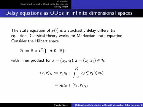
Delay equations as ODEs in infinite dimensional spaces

The state equation of y(·) is a stochastic delay differentialequation. Classical theory works for Markovian state-equation.Consider the Hilbert space

H := R× L2([−d , 0];R

),

with inner product for x = (x0, x1), z = (z0, z1) ∈ H

〈x , z〉H := x0z0 +

∫ 0

−dx1(ξ)z1(ξ)dξ

= x0z0 + 〈x1, z1〉L2



Sticky wages

SetX (t) =

(X0(t),X1(t)

):=(y(t), y(t + ξ)|ξ∈[−d ,0]

),

X (t) is an element of H for all t ∈ [0,+∞). Let X satisfy

dX (t) = AX (t)dt + CX (t)dZ (t), X (0) = (y0, y1) ∈ H

with

A(x0, x1) :=(µyx0 + 〈α(·), x1(·)〉L2 , x ′1(·)

),

C (x0, x1) := (x0σy , 0)

Then the original problem is equivalent to the control problem withstate X in the infinite dimensional space H(see Gozzi-Marinelli ’04).



Sticky wages

Our result

Theorem

The value function V0 is

V0(W , x0, x1) := f γ∞Γ1−γ

1− γ,

where

f∞ := (1 + δk1γ−1)ν,

ν :=γ

ρ+ δ − (1− γ)(r + δ + κ>κ2γ )

> 0.

Γ := W0 + Gx0 + 〈H, x1〉L2 ≥ 0,



Sticky wages

The optimal strategies are

c∗(t) := f −1∞ Γ∗(t)

B∗(t) := k−bf −1∞ Γ∗(t)

θ∗(t) :=(µ− r)Γ∗(t)

γσ2− Gσyy(t)

σ,

where Γ∗(t) := W ∗(t) + GX0(t) + 〈H,X1(t, ·)〉L2 .We have

dΓ∗(t)

Γ∗(t)=[r + δ +

1

γ(µ− r

σ)2

− f −1∞(1 + δk−b

)]dt

+µ− r

γσdZ (t).



Sticky wages

First findings

with no-labor risk (σy = 0), the optimal ratio θ∗

Γ∗ and c∗

Γ∗ areconstant, as in the Merton model

taking α = 0, we recover Dybvig-Liu result

taking α 6= 0, we recover Dybvig-Liu result, but substitutingto the optimal total wealth Λ∗ (financial wealth + humancapital) of Dybvig-Liu the quantityΓ∗(t) = W ∗(t) + G (t)X0 + 〈H(t, ·),X1(t, ·)〉Λ∗ and Γ∗ evolve with the same dynamic



Sticky wages

Sketch of the proof

Guess the value function to be

V (W0, x0, x1) := f γ∞(W0 + Gx0+〉H, x1〈L2)1−γ

1− γ,

putting V in the HJB equation, gives equations for f ,G ,H

solving these equations, we get that f ,G ,H are the constantas in the main Theorem

V is C1,2

Verification Theorem holds and the optimal feedbackstrategies are admissible



Sticky wages

Thank you for your attention



Sticky wages

References

Benzoni, L., Collin-Dufresne, P. and Goldstein, R. (2007)Portfolio Choice over the life-cycle when the stock and labormarkets are cointegrated in The Journal of Finance, 62, 5,pp.2123-2167

Dybvig, P.H. and Liu, H. (2010) Lifetime consumption andinvestment: retirement and constrained borrowing in Journalof Economic Theory, 145, pp. 885-907

Farhi, E. and Panageas, S. (2007), Saving and investing forearly retirement: a theoretical analysis, in Journal of FinancialEconomics 83, pp. 87-121



Sticky wages

Gozzi, F. and Marinelli, C. (2006), Stochastic optimal controlof delay equations arising in advertising models, in StochasticPartial Differential Equations and Application VII. Lect. NotesPure Appl. Math., 245, pp. 133 - 148. Chapman &Hall/CRC, Boca Raton

Meghir, C. and Pistaferri, L. (2004) Income variance dynamicsand heterogeneity, Econometrica, 72, 1, pp. 1-32


optimal portfolio choice with path dependent labor income ...€¦ · optimal portfolio choice with...

Documents