modelling ngong river final project 2010
DESCRIPTION
ngongTRANSCRIPT
JOMO KENYATTA UNIVERSITY OF
AGRICULTURE AND TECHNOLOGY.
DEPARTMENT OF CIVIL, CONSTRUCTION AND
ENVIRONMENTAL ENGINEERING.
MODELLING WATER QUALITY OF
THE NGONG’ RIVER
PREPARED BY:
KRHODA MICHAEL OKOYE
(E25-0177/05)
FINAL YR PROJECT FOR BSC. CIVIL, CONSTRUCTION
AND ENVIRONMENTAL ENGINEERING.
23RD November 2010

MODELLING WATER QUALITY OF THE NGONG’ RIVER
2 E25-0177/05
ACKNOWLEDGMENTS
I take this opportunity to thank the Almighty God for health and provision throughout this
period as I worked on this project. Let this be testament of His goodness for His glory both in
this life and in the life eternal.
I thank Marian Kioko at NEMA for the information and assistance that she afforded me during
the initial stages of the project. I thank Isaac Muraya at City Hall for the background
information about the Nairobi River Basin Programme. I thank Mrs Kibetu from Jomo
Kenyatta University of Agriculture and Technology (JKUAT) Dept. of Construction, Civil and
Environmental Engineering, for her wise council throughout the period that I consulted with
her about the project work. I thank Mr Kibe from the Civil Environmental Lab for the
assistance in carrying out the testing of the samples. I thank Wambia Waigwa and Paddy
Mulweye for their selfless help during sample collection.
Thank you Prof. Krhoda and Mrs Krhoda for everything you have done for me to make this
possible.

MODELLING WATER QUALITY OF THE NGONG’ RIVER
3 E25-0177/05
DECLARATION
“I KRHODA MICHAEL OKOYE do solemnly declare that this report is my original work and to the best of my knowledge, it has not been submitted for any degree award in any University or Institution.”
Signed……………………………… (Author)
Date……….………………………..
E25-0177/05
CERTIFICATION
“I have read this report and approve it for examination.”
Signed……………………………………… (Supervisor) Date………….……………………………..
MRS. KIBETU.

MODELLING WATER QUALITY OF THE NGONG’ RIVER
4 E25-0177/05
Table of Contents List of abbreviations: ................................................................................................................... 7
MODELLING THE WATER QUALITY OF THE NGONG' RIVER. ....................................... 8
1. INTRODUCTION ............................................................................................................... 8
1.1 Background: ............................................................................................................... 8
1.2 Study Justification: ..................................................................................................... 9
1.3 Problem Statement: .................................................................................................. 10
1.4 Objectives: ................................................................................................................ 10
1.4.1 Overall objectives: ........................................................................................... 10
1.4.2 Specific objectives: .......................................................................................... 10
1.5 Research Hypothesis: ............................................................................................... 10
1.6 Limitations of the research: ...................................................................................... 11
2. LITERATURE REVIEW .................................................................................................. 13
2.1 Context of modelling ................................................................................................ 13
2.2 General geographic information ............................................................................... 15
2.3 General pollution information .................................................................................. 17
2.4 Description of the river basin ................................................................................... 20
2.4.1 The IPU section ............................................................................................... 20
2.4.2 The CPU section .............................................................................................. 21
2.4.3 The MPU section ............................................................................................. 23
2.5 Hydrological measurements ..................................................................................... 24
2.6 Nutrients in the Ngong River.................................................................................... 25
2.6.1 Nitrogen compounds ........................................................................................ 25
2.6.2 Phosphorus compounds ................................................................................... 30
2.7 Results from previous studies and the gap that exists .............................................. 31
3. RESEARCH METHODOLOGY ...................................................................................... 36
3.1 Orientation ................................................................................................................ 37
3.1.1 Data collection methods................................................................................... 37
3.1.2 Measuring stream flow: ................................................................................... 37
3.1.3 Sampling: ......................................................................................................... 39
3.1.4 Materials and methods of water quality analysis ............................................. 39
3.2 Formulation of relations between variables and parameters ..................................... 50
3.3 Non-dimensionalization ........................................................................................... 50

MODELLING WATER QUALITY OF THE NGONG’ RIVER
5 E25-0177/05
3.4 Solution of model equations ..................................................................................... 51
3.5 Preliminary test application ...................................................................................... 51
3.6 Model Verification ................................................................................................... 51
3.7 Reiteration of steps 2-6 ............................................................................................. 51
3.8 Implementation ......................................................................................................... 52
4. DATA COLLECTION/ SAMPLING ............................................................................... 53
4.1 Catchment characteristics ......................................................................................... 53
5. SAMPLE RESULTS AND DATA ANALYSIS .............................................................. 59
5.1 Longitudinal Profile.................................................................................................. 59
5.2 Cross-sectional Profile .............................................................................................. 60
5.3 Biochemical Oxygen Demand .................................................................................. 60
5.4 Ammonia .................................................................................................................. 62
5.5 Nitrite ....................................................................................................................... 64
5.6 Nitrates ..................................................................................................................... 66
5.7 Phosphates ................................................................................................................ 69
5.8 Comparison of results from 2003 with 2010 ............................................................ 71
6. MODELLING ................................................................................................................... 75
6.1 THE WATER QUALITY MODEL ......................................................................... 75
6.1.1 Model Network ................................................................................................ 75
6.1.2 Model Inputs: ................................................................................................... 75
6.1.3 Hydraulic Calculations: ................................................................................... 78
6.1.4 Water quality calculations ............................................................................... 79
6.2 Solution to model equations and Preliminary test application: ................................ 83
6.2.1 BOD ................................................................................................................. 83
6.2.2 Ammonia ......................................................................................................... 83
6.2.3 Nitrate .............................................................................................................. 83
6.2.4 Nitrite ............................................................................................................... 84
6.2.5 Phosphates ....................................................................................................... 84
6.3 Model Verification and implementation: .................................................................. 84
6.4 Accounting for pollution input into the river: ........................................................... 89
6.5 Capabilities and Limitations of the Water Quality Model ........................................ 89
6.6 Discussion: ............................................................................................................... 90
6.7 Conclusions: ............................................................................................................. 90
7. RECOMMENDATIONS AND WAY FORWARD ......................................................... 91
8. REFERENCES: ................................................................................................................ 92

MODELLING WATER QUALITY OF THE NGONG’ RIVER
6 E25-0177/05
9. APPENDICES: ................................................................................................................. 95
9.1 Budget: ..................................................................................................................... 95
9.2 Working schedule: .................................................................................................... 96
9.3 The tabulated results from NRDP- Phase II, UON/UNEP project, Feb- Nov 2003, Final report: ........................................................................................................................... 97
9.4 The plotted results from NRDP- Phase II, UON/UNEP project, Feb- Nov 2003, Final report: ........................................................................................................................... 98
9.5 Manning’s co-efficient (Chow, 1959): ..................................................................... 99
9.6 Summary output from regression analysis for modelling: ...................................... 100
9.6.1 BOD ............................................................................................................... 100
9.6.2 Ammonia ....................................................................................................... 101
9.6.3 Nitrates .......................................................................................................... 102
9.6.4 Nitrites ........................................................................................................... 103
9.6.5 Phosphates: .................................................................................................... 105
9.7 SISMOD OPERATION ......................................................................................... 106

MODELLING WATER QUALITY OF THE NGONG’ RIVER
7 E25-0177/05
List of abbreviations: NRBP: Nairobi River Basin Programme
UNEP: United Nations Environmental Programme
UN- HABITAT: United Nations Habitat
UoN: University of Nairobi
AWN: Africa Water Network
TN: Total Nitrogen
TP: Total Phosphates
CBD: Central Business District
IPU: Individual Polluting Unit
CPU: Collective Polluting Unit
MPU: Mega Polluting Unit
NO3-: Nitrate ion
NO2-: Nitrite ion
NH4-: Ammonium ion
N2: Molecular nitrogen
N2O: Nitrous oxide
PO43-: Phosphate ion
HCl: Hydrochloric acid
NaOH: Sodium hydroxide
H3BO3: Boric acid
SISMOD: Simple Stream Model

MODELLING WATER QUALITY OF THE NGONG’ RIVER
8 E25-0177/05
MODELLING THE WATER QUALITY OF THE NGONG' RIVER.
1. INTRODUCTION
1.1 Background: If real life problems are attacked using mathematics, a ‘translation’ is needed to put the subject
into mathematically tractable form (Mooney, 1999). Modelling is the description of an
experimentally verifiable phenomenon by means of the mathematical language where we have
2 classes of quantities:
• Variables: we distinguish between dependent and independent variables.
• Parameters: these are used to link variables to each other. Are either constant or
adjusted by the experimenter.
Water quality models are important decision support system tools for water pollution control,
study of the health of aquatic ecosystems and assessment of the effects of point and diffuse
pollution (Bende-Michl et al, 2009). A mathematical stream water quality model with the
following specifications is used:
The model is mechanistic. This means that it is derived from the mathematical abstraction of
physical phenomena such as mass balance, transport and reaction kinetics, to allow the users to
construct mass balances on stream locations with discharges, diffuse loads and stream
junctions. A mechanistic model also provides the opportunity to give the users an introduction
to the essential processes in stream pollution and purification (Erturk et al., 2006).
The model is steady state. This means that can only characterize a system after it has reached
the steady state, and is therefore relatively easy to run (Erturk et al., 2006).
The model is a spatial model. It considers the spatial heterogeneity of the system. It solves the
water-quality related equations in one dimension that is defined along the stream in flow
direction (Erturk et al., 2006).
The model solves the water quality equations analytically. Analytical models use the exact
solution of systems equations and are therefore applicable to special simple cases, where an
analytical solution exists for the model equations.
According to the United Nations Environmental Programme, Nairobi Rivers are increasingly
chocking with uncollected garbage, human waste from informal settlements; industrial waste in
the form of liquid effluence and solid waste; agrochemicals, and other waste, especially petro-

MODELLING WATER QUALITY OF THE NGONG’ RIVER
9 E25-0177/05
chemicals and metals from micro-enterprises – the “Jua-kali”; and overflowing sewers. These
pollutants change in position and momentum as they flow within the water body. Of particular
concern is the Ngong’ River, a tributary of the Nairobi River.
This pollution situation has occasioned spread of water-borne diseases, loss of sustainable
livelihoods, loss of biodiversity, reduced availability and access to safe potable water, and the
insidious effects of toxic substances and heavy metal poisoning which affects human
productivity.
The Nairobi River Basin programme (NRBP) was established as a multi-stakeholder initiative
to bring together the Government of Kenya, UNEP, UN-Habitat, UNDP, the private sector and
civil society with a vision to restore the riverine ecosystem with clean water for the capital city
and a healthier environment for the people of Nairobi. One of the objectives of NRBP was to
rehabilitate, restore and manage the Ngong’ River ecosystem. Phase I of the programme
(October 1999 to March 2000) constituted a situation assessment of water quality, status and
impact of pollution, a project that was implemented by the Africa Water Network (AWN).
Phase II of the NRBP was conducted to the Ngong/Motoine river to provide information for
the pilot project to identify major point sources of pollution.
1.2 Study Justification: The purpose of this study is the development of a water quality model and to determine the
biological and chemical characteristics and the concentration of constituents in the river water
at different locations along the course of the river and provide data for an understanding of the
nature of the river water is essential in the management of environmental quality.
Freshwater management challenges are increasingly common. Limited resources of the Ngong’
River are allocated between agricultural, municipal and industrial use. It is thus necessary to
determine pollution generation, discharge, flows and in-stream water quality under the current
uses of the water.
An analysis of the loading data of the Ngong’ River will allow the researcher to suggest any
pollution reduction measures that can be undertaken to restore the quality of the water of the
Ngong’ River.
The section of the Ngong’ River to be considered is the profile from Karaini Dam to a location
where it drains out to the Industrial Area at Outer Ring road bridge. This area is of particular
interest in order to determine the effect of the presence of informal human settlement and
industrial processes on the quality of the water of the Ngong River flowing through the area.

MODELLING WATER QUALITY OF THE NGONG’ RIVER
10 E25-0177/05
Increasing industrialisation and the growth of large urban centres have been accompanied by
increases in the pollution stress on the aquatic environment.
1.3 Problem Statement: Models are necessary to monitor and analyse the current pollution levels of the Ngong’ River
and to determine the ability of the river to naturally dilute the pollutants because it directly
affects the livelihoods, biodiversity and availability of potable safe water for its environs.
1.4 Objectives: Objectives are broken down into overall and specific objectives.
1.4.1 Overall objectives: a. To investigate the current quality of the water in the Ngong’ River.
b. To carry out water quality modelling.
1.4.2 Specific objectives: a. To obtain samples of water from points along the longitudinal profile of the
Ngong’ River and carry out an analysis of the quality of the water.
b. To identify the level of pollutants in the Ngong’ River.
c. To determine the change in water quality by comparison of concentration of
BOD and nutrient constituents along the Ngong' River profile.
d. To determine the sources of these pollutants in terms of activities or agents
such as industries, informal settlements.
e. To undertake water quality modelling for the Ngong’ River.
f. To determine the monitoring needs and suggest possible pollution reduction
measures that can be taken to restore the quality of the water in the Ngong’
River.
1.5 Research Hypothesis: The concentrations of pollutants in the Ngong’ River has risen since AWN did their assessment
for NRBP in February- November 2003.

MODELLING WATER QUALITY OF THE NGONG’ RIVER
11 E25-0177/05
1.6 Limitations of the research: a) Scope of research: the scope of this research project is limited to
a. Biological Oxygen Demand (BOD)
b. Total Nitrogen (TN) - nitrates, nitrites and ammonia.
c. Total phosphates (TP)
b) The water quality modelling will be done through the use of the diffusion equations or
finite difference methods. The prototype is a continuum of constituents and processes.
Simulation of such a system on a computer requires representation in a discrete
fashion.
c) Sampling points shall be limited to positions at the following locations:
1. Sample site 1: Kariani Dam
Objective: identification of baseline conditions in the water course system
2. Sample site 2: Jamhuri Park dam outlet
Objective: selection of a point to determine the change in baseline conditions
before entry into Kibera Slum.
3. Sample site 3: Kibera bridge
Objective: selection of a point to evaluate the effect of informal human
settlement on the quality of the river water.
4. Sample site 4: weir at the outlet to Nairobi Dam
Objective: to assess and determine the difference in the water quality after
stabilisation in Nairobi Dam.
5. Sample site 5: Dunga Road Bridge.
Objective: selection of a point to determine the extent and effect of waste
discharges from industrial establishments
6. Sample site 6: Outer-ring Road Bridge

MODELLING WATER QUALITY OF THE NGONG’ RIVER
12 E25-0177/05
Objective: selection of a point to determine the extent and effect of waste
discharges from industries.
d) Model verification will be done with only 1 test data due to temporal constraints.

MODELLING WATER QUALITY OF THE NGONG’ RIVER
13 E25-0177/05
2. LITERATURE REVIEW
2.1 Context of modelling Water quality changes in rivers are due to physical transport processes and biological,
chemical, biochemical, and physical conversion processes.
The above processes in the water phase are governed by a set of extended transport equations
that can be represented conceptually in the diagram below (Reichert et al., 2001):
=+ + +
Diagram 2.1: shows the transportation process of pollutants in a natural water system.
Advection is the transport mechanism of a substance or the conserved property, by a fluid, due
to the fluid’s bulk motion in a particular direction e.g. the transport of pollutants in a river. The
motion of the water carries these impurities downstream. The fluid motion in advection is
described mathematically as a vector field and the material transported is typically described as
a scalar concentration of substance. Advection requires currents and thus can only take place in
fluids. The advection equation is the partial differential equation that governs the motion of the
conserved scalar as it is advected by a known velocity field.
Diffusion is the spread of particles through random motion from the regions of higher
concentration to regions of lower concentrations. The time dependence of the statistical
distribution in space is given by the diffusion equation which is a partial differential equation
which describes density fluctuations in a pollutant undergoing dispersion.
Conversion is the process by which the pollutant under investigation is broken down by
biological, chemical, biochemical, and physical conversion processes.
A modification of a mathematical stream water quality model called SISMOD (Simple
Stream Model) with the following specifications is used (Erturk et al., 2010):
The model is mechanistic. This means that it is derived from the mathematical abstraction of
physical phenomena such as mass balance, transport and reaction kinetics, to allow the users to
construct mass balances on stream locations with discharges, diffuse loads and stream
junctions. A mechanistic model also provides the opportunity to give the users an introduction
to the essential processes in stream pollution and purification.
Change in concentration
Change due to advection
Change due to diffusion or dispersion
Change due to conversion processes
MODELLING WATER QUALITY OF THE NGONG’ RIVER
14 E25-0177/05
The model is steady state. This means that can only characterize a system after it has reached
the steady state, and is therefore relatively easy to run.
The model is a spatial model. It considers the spatial heterogeneity of the system. It solves the
water-quality related equations in one dimension that is defined along the stream in flow
direction.
SImple Stream MODel (SISMOD) is modelling software that can conduct simple hydraulic
and water quality calculations along a stream in flow direction. It is easy to use and is designed
such a way that it can be integrated with other software (Erturk, 2009).
The water quality model developed in this study is a preliminary model adapted from SISMOD
that mainly aims at supporting the water quality assessment. For the purposes of this
experiment the modelling process will be applied.
SISMOD solves the relevant equations analytically- Analytical models use the exact solution
of systems equations and are therefore applicable to special simple cases, where an analytical
solution exists for the model equations; however some intermediate calculations are conducted
using numerical algorithms. Water quality calculations are conducted step by step and serially
with hydraulic calculations. The model will simulate five water quality variables including
biochemical oxygen demand, ammonium nitrogen, nitrate nitrogen and phosphate phosphorus
for primarily aerobic and conditions.
There are three types of reaches in SISMOD model network. These are defined as;
a) Headwater reach: the beginning of the streams or in model network they constitute the
beginning of the model network. In a model network several headwater reaches can be
defined.
b) Standard reach: a regular reach with no specific characteristic
c) End reach: the reach where the model network ends and all the flow goes out of the
systems. In the model network, there can only be one end reach.
Other definitions that are important in the operation of SISMOD are:
a) Diffuse Load without Flow: These are the diffuse source loads without flow that are
entering the stream reach and are in unit of kg.km-1.day-1. Diffuse source loads
without flow should be defined for each stream reach. If there are no diffuse sources
without flow for a water quality parameter in a stream reach, than it should be defined
as zero kg.km-1.day-1.

MODELLING WATER QUALITY OF THE NGONG’ RIVER
15 E25-0177/05
b) Diffuse Load with Flow: These are the diffuse source loads with flow that are entering
the stream reach. For diffuse source loads with flow, flows and the concentrations of
each simulated water quality parameter should be defined. Diffuse source loads with
flow should be provided to the model for each stream reach. If there are no diffuse
sources with flow for a water quality parameter in a stream reach, than it should be
defined as zero.
2.2 General geographic information There are three main tributaries that flow through Nairobi City’s Central Business District
(CBD), namely River Nairobi, River Mathare and River Ngong, all of which are subjected to
extreme levels of pollution ranging from agricultural fertilizers and raw domestic sewage, to
industrial waste. A general map of Ngong' River showing the relative positions of the sampling
stations along the profile is shown on the page that follows.
Diagram 2.2: Map of Ngong' River and the sampling stations along the profile of the river.

MODELLING WATER QUALITY OF THE NGONG’ RIVER
16 E25-0177/05
In most cases, solid and liquid waste from these sources are discharged directly into the river
system having undergone no treatment whatsoever, thereby severely damaging the river
ecology as well as posing severe risks to human health. The rivers themselves are now
considered an environmental health hazard due to the high concentrations of chemical and
bacteriological toxic waste. Despite this, nearly half of the urban population are at one time or
other, dependent on them as a source of water for domestic use and in the worst cases, for
drinking (Kahara, 2002).
Most heavily affected are the urban poor, who are also reliant on the sewage lines for irrigation
of vegetables and other crops that they grow within the city as a source of income.
Unfortunately, many of the city's sewage lines are deliberately damaged or blocked in order to
obtain the nutrient rich water for agriculture. Untreated industrial effluents, raw sewage and
waste (liquid and solid) from human settlements situated along the rivers have severely
impacted the rivers quality and quantity, resulting in eutrophication, proliferation of hazardous
microbes and acute chemical stress on the aquatic ecosystem (Kahara, 2002).
Increased discharges of mostly untreated or poorly treated municipal waste water from sewage
systems in the city have plainly turned these rivers into open sewers. Industries within Nairobi
that have very poor waste treatment, if any, are discharging their waste waters into the existing
municipal sewerage system and/or directly into the rivers. Non-biodegradable waste
accumulates, thus overloading the system effectively reducing its self-purification capacity
(NRBP-UNEP, 2000). The water supply of Nairobi was initially designed to serve a population
of a few thousands; however, it has become increasingly clear that the system is inadequate to
serve the current population of over two million.
Considering the number of projects involved, it is a national dilemma as to if there has been
any improvement at all.
A picture of the polluted Ngong' River is in the page that follows:

MODELLING WATER QUALITY OF THE NGONG’ RIVER
17 E25-0177/05
Diag 2.3: a heavily polluted Ngong' River coursing through Nairobi’s Eastlands area after
Industrial area (October 2008).
2.3 General pollution information Nairobi River has several tributaries, namely Motoine/ Ngong River, Nairobi River and the
Mathare River. In a study conducted for the Nairobi River Basin Project in the year 2000, the
sources (namely, Ngong' and Dagoretti forest, Ondiri/Kikuyu wetlands and Mathare catchment
area respectively) were observed as being generally clean and free of pollution. Farmers around
the Ondiri Swamp at the source of Nairobi River, use the water to irrigate land and plant
vegetables as well as other crops. They also use the water for drinking and watering their
animals. Pollution of the rivers becomes most apparent as it flows through the slum areas and
finally reaches alarmingly high levels in the industrial areas.
It is important to note that almost half of the urban population live in unplanned settlements
(slums), which for the most part lack basic water and sewerage facilities. It is not surprising
that these communities are established next to the rivers (Ndede, 2002).
Numerous studies have already been conducted over the past two decades (see Ohayo et al.
1996, Wandiga 1996, Olago et al. 2000, Issaias 2000, Kithaka 2001), to assess the rivers’ water
quality and results indicate that the levels of pollution are rising progressively between the
source and the industrial area. In each case study the main reasons for pollution in the rivers
were identified, and all agree on the following;

MODELLING WATER QUALITY OF THE NGONG’ RIVER
18 E25-0177/05
1. Non-implementation of legislation to protect urban water resources.
2. Intentional or accidental blockage of sewer lines and manholes for various reasons.
3. Absence or poor planning of settlements along rivers and water bodies.
4. Acute shortage of funds in Local Government Authorities to sort out the problems.
The most important consideration of the problem lies in its diversity, and the fact that the range
of river pollution is very broad in terms of pollutants and the area affected (NRBP- Phase II).
Various studies have been conducted on the Ngong' River and its environs, and from them,
attempts have been made to develop a strategy through which the problem can be classified
and adequately tackled.
Although much of the data that has been collected thus far has tended to be both spatially and
temporally disjointed (due to lack of a basic monitoring criterion), it has provided a enough
base to assume a general pollution trend. The data collected presents the possibility that there
may be three or more basic categories of anthropogenic pollution sources or groups of
polluters, from the time the rivers begin to be of financial or social use, till they depart from the
CBD. Each category or group of polluter presents a set of problems, which are by comparison,
very diverse from the other. No attempts have been taken before to detail different
methodologies that can capture the diverse pollution categories adequately. It is appreciated
here that for sufficient statistical analysis, the sampling methodology and overall long term
monitoring design should be adjusted to provide an objective and realistic basis for assessment
(Kahara, 2002).
It becomes clear that no matter how much effort is placed on rectifying the pollution at one
section or category of pollutants; this strategy will ultimately be cancelled by the other groups
of polluters .Each case is different and therefore requires a slightly modified approach. While it
would be an immense and economically unworkable task to deal with individual problems, the
categories of pollutants would each contain those polluters displaying similar traits in terms of
demography, types of pollution released, socio-economic structure and overall effect on the
ecology (Kahara, 2002).
The basic groups herein referred to as Polluting Units, can be divided theoretically into the
following (Kahara, 2002):
1. Individual Polluting Units (IPUs),
which are found in the upper reaches of the river basin, where the population densities
and population growth rates are relatively low. Their main activities include crop

MODELLING WATER QUALITY OF THE NGONG’ RIVER
19 E25-0177/05
farming and animal husbandry which usually results in low to medium pollution due
to limited agricultural chemical and fertilizer usage. Other problems such as high
turbidity may occur due to soil erosion arising from deforestation and poor land
management practices. Removal of riparian vegetation could also increase risks of
flash floods downstream. Many of the problems in such areas can be solved through
education and awareness programmes to suit the needs of the area and to improve land
management.
2. Collective Polluting Units (CPUs),
which are usually found within the city limits, and are characterized by high
population density and high growth rates, mainly resulting in unplanned settlements,
which encroach on the river-banks. The level of pollution produced in such areas can
be equated to several IPUs both in quantitative and qualitative effect on the river
ecology. Here the main pollutants are domestic organic waste (equivalent in
composition to fertilizer/manure), and large amounts of non-biodegradable solid waste
with high plastic content. The population in such areas is highly dynamic and
therefore it may be difficult for awareness/ education campaigns to effect sustainable
changes in residents’ beharviour. CPUs may require a more technical approach such
as planning connections to main sewerage lines and the establishment of definite
guidelines that can be enforced by the Community Based Organisations (CBOs) in the
area. These areas also require a greater support and cooperation from the Local
Authorities to be able to plan effectively.
3. Mega-Polluting Units (MPUs),
Include large-scale manufacturers and industries, which discharge pollutants in vast
quantities and high concentrations directly into the river water. This may be done
intentionally or as a result of faulty sewer lines, which require unblocking or
upgrading. The pollutants produced here are usually rich in toxic chemicals and heavy
metals, as well as high concentration of organic waste. It is expected that production
rate may increase to cater for an overall growing population (market), thus resulting in
more pollution being released. These are cases of non-implementation of legislation
governing waste treatment before being discharged into water sources. In some areas
the main problem occurs due to blocked, overflowing sewers, a problem which simply
requires rectification by the Local Authorities. The process of unblocking the sewers
is also hampered by the lack of facilities, therefore it could be suggested that the
industries take it upon themselves to contribute to the correction of sewer breakages
and take responsibility.

MODELLING WATER QUALITY OF THE NGONG’ RIVER
20 E25-0177/05
2.4 Description of the river basin The study river subject to this project is the NGONG RIVER with a total catchment area from
the source to the confluence with Nairobi River of about 127 km2. The source of Ngong' River
is Motoine swamp and Dagoretti forest, possibly from springs issuing between lava flows with
differing porosities and permeability.
The basin comprises of various land use types, namely forest, grasslands, farmlands, limited to
flood plains and around the dam; and built area, including buildings and roads. The following
are descriptions of the river basin specifically as it relates to the proposed Polluting Units. The
entire river basin is about 42.3 km long and narrow.
2.4.1 The IPU section The IPU section stretches on the upper sections of Ngong/Motoine River. From the source, the
river flows through a series of four man-made dams before River Motoine crosses Ngong Road
Bridge, and two larger dams at the Race Course. A small tributary from Ngong forest joins the
Motoine River near the Race Course, before it flows into Nairobi Dam marking the southern
boundary of the Kibera informal settlement (CPU section).
Up to the dam where the CPU section begins, the river basin is about 26.7 km long and not
more than 5 km at its widest breadth. The river channels are steep, V-shaped cross-sections as
a result of the continued uplift and deposition of lava and tuff and deeply incised and or re-
excavated within their own valleys.
Erosion and sediment deposition in the upper reaches
Sediment is produced wherever soil is exposed to rainfall energy and flowing water. Erosion
from farms, gardens, roads as well as footpaths are common. Other sediment sources include
construction sites, earth-lined channels and mass wasting processes including avalanche,
landslides and mudflows. Most of these sediment drains into the dam, reducing the storage
capacity of the dam. The problem of erosion needs to be addressed throughout the river basin,
but most urgently, in the upper reaches where deforestation and encroachment onto the riparian
way leave has led to heavy soil erosion.
Activities along the river
The Motoine River rises from Riu Swamp and is heavily used in the settled Dagoretti area. As
the river flows eastwards (mainly underground) for most of its course, farmers in the valley

MODELLING WATER QUALITY OF THE NGONG’ RIVER
21 E25-0177/05
impound its water for irrigation agriculture and several other domestic uses. The water colour
in this section of the river is mainly red due to the soil characteristics of the area. Other
polluting activities include dairy farming and abattoirs. Therefore, the Motoine River starts
receiving agrochemical pollution right from its head water in the Dagoretti area, and picks
other forms of pollution as it flows through the Ngong' Forest and the Kibera area. A second
IPU section may exist after the Industrial area, approximately 20 km up to the confluence with
the Athi River.
2.4.2 The CPU section The stretch from the Nairobi dam outlet to the confluence with Nairobi River is about 21.0 km
long. From the Nairobi Dam spillway right through the Langata Road Bridge flows through
concrete and lined channels. River-bank erosion was noted only at the Langata Road Bridge
where there was no concrete lining. The impact of concrete lining on groundwater recharge to
the adjacent floodplain and discharge to the stream during the dry season are not known,
however the lack of lateral connectivity is very likely to have an effect on the water quality.
Further downstream of the confluence down cutting has incised the river valley to about 15 to
30m deep.
Hydrological regime of Nairobi dam
The Nairobi dam was constructed in the late 1940's as a source of fresh drinking water for the
city of Nairobi. The Nairobi Dam is shallow; at the time constructed it had a surface area of
about 356,179 m2 and a volume of 98,422m3. The average depth of the dam was 2.76m. The
dam inlet is about 1700m while the dam crest is about 1680m above mean sea level. The dam
is currently heavily silted by sediments from erosion and solid waste dumped at various places
to reclaim land for agriculture. Water hyacinth (Eicchornia crassipes) as well as various other
aquatic macrophytes, such as common reeds and bulrushes, have infested the water body
disrupting fisheries and recreation (Issaias 2000).
Over the past decade the dam has reached hyper-eutrophic levels and is generally of little
socio-economic use to the city, despite its unique position in the CBD (Kahara, 2002). It is
nevertheless an essential part of the river course as a number of biochemical reaction take place
within the anaerobic water column.
Over dam precipitation is about 875mm per annum on a surface area of 356,179 m2. The
evaporation rate is about 1750mm per annum as temperature and wind velocity increase while

MODELLING WATER QUALITY OF THE NGONG’ RIVER
22 E25-0177/05
relative humidity decreases towards the lower part of Nairobi (Ohayo et al. 1996).
Evapotranspiration from the water hyacinth may be higher than potential evaporation. An
estimate of 1.13 times the rate of potential evaporation has been adopted for the water balance
calculation.
The densely populated settlements beside the dam are the most important source of both solid
and liquid pollution, but it is possible that the river can purify most of the domestic pollutants
naturally given adequate amounts of time. Solid waste is much more difficult to deal with and
this has led to a dramatic decrease in the residence time within the reservoir. Change on water
storage in the dam may be measured by continuous recording of water levels over the years.
Currently, there is no record.
However for Nairobi Dam rearranging and solving for outflow through Ngong River, we
obtain:
Qm = P + R – dS – E Equation 2.1
Where Qm = discharge
P = precipitation
dS = change in storage
E = evapotranspiration
Rearranging and simplifying, the change in storage, dS, is negligible. It is important to note
that none of the studies have as yet properly addressed the problem of water and mass balances
for the rivers reservoirs, and most are simply estimates from old data. For the purpose of
management it is suggested that a clear record of the reservoir mass/water balance be kept in
order to monitor the input of pollutants and the changes undergone during their residence in the
dams.
Activities along the Nairobi dam to the confluence with Nairobi River
The Motoine River is the main inlet into the Nairobi Dam, but other streams and springs
discharge into the Dam as well (Ndede 2002). Runoffs from the impervious surfaces, such as
iron sheet roofs of the Kibera settlement also contribute significant amounts of flow into the
Dam, especially during rainstorms. The amount of discharge from within the catchment into
the Dam at base flows is about 0.5 cumecs, including underground seepage. The amount
leaving the Dam through the spillway as the Ngong River is variable. During dry years, it

MODELLING WATER QUALITY OF THE NGONG’ RIVER
23 E25-0177/05
becomes a mere trickle, but when there are heavy rains, it floods. In November 2001, the flow
from spillway was measured at 0.2 cumecs (Ndede 2002).
Various activities such as car washing, small-scale industry and urban farming have been
observed in this area, all of which are dependent on the river water both as a source as well as a
drainage system.
Due to lack of a waste management mechanism for Kibera slum, the Motoine River system has
become a natural receptacle for all the uncollected waste emanating from the area. Dumping of
solid waste is serious at bridges and crossing points. Drainage systems within the slums have
also become channels of domestic sullage from the unserviced informal settlements. These
polluting outfalls have made the water quality of Motoine to deteriorate further as it flows
through Kibera into the Nairobi Dam. Eutrophication of the Nairobi Dam is largely responsible
for the water hyacinth infestation. The Motoine leaves the Nairobi Dam as the Ngong River at
the spillway, and data shows that it undergoes some natural purification process as it cascades
through the concrete channel in the South C area and the Industrial Area. This situation does
not persist for long, as more serious forms of pollution are released into the Ngong' River in the
Industrial Area (Ndede, 2002).
2.4.3 The MPU section Downstream of the Nairobi dam and starting with the weir, the river channel is for the most
part channelised as it flows through the Industrial area. The stream in this section is fast
flowing and much of the riparian vegetation has been removed resulting in the exposure of the
river to heavy pollution from runoff. The channels are usually wide and shallow with concrete
lining, and several bridges cross over the river beneath which a lot of garbage is dumped. The
distance covered by this section is quite short, between 2 and 4 km (Kahara, 2002).
Activities along the channelised river section
Just before the Industrial area, the river passes through another CPU section (Mukuru slum),
where various activities such as several small scale industries have been set up along the river
bank. Car garages and other large industries have been observed discharging their effluent
directly into the river. Pollutants ranging from automobile oils, pigments detergents and
unidentified solid material are found emerging from broken sewer lines. As the river departs
the MPU section, the discharge rises quite steeply and it has been suggested that this is a result
of direct sewage input.
MODELLING WATER QUALITY OF THE NGONG’ RIVER
24 E25-0177/05
The section downstream of the confluence with the Nairobi River is characterized by low
human activity apart from some agriculture towards it’s confluence with the Athi river. Several
tributaries join the river at this stage and the Dandora Sewage Treatment Works also discharge
treated sewage into the waters.
2.5 Hydrological measurements
Proper interpretation of the import of water quality variables in a sample taken from a river
requires information of the discharge of the river at the time and place of sampling. In order to
calculate the mass flux of chemicals in the water, (the mass of a chemical variable passing a
cross-section of the river in a unit time), a time series of discharge measurement is critical.
The flow rate or discharge of a river is the volume of water flowing through a cross section in a
unit of time and is usually expressed as m3/s. It is calculated as the product of average velocity
and cross-sectional area but is affected by hydraulic variables such as water depth, alignment
of the channel, gradients and roughness of the river bed. Discharge may be estimated by the
slope-area method, using hydraulic variables in one of the variations of the Manning’s equation
which, although developed for conditions of uniform flow in open channels, may give an
adequate estimate of the non-uniform flow which is usual in natural channels.
Velocity usually varies as a parabola from zero at the channel bottom to a maximum near the
surface. It has been determined empirically that for most channels the velocity at six-tenths of
the total depth below the surface is a close approximation to the mean velocity at the vertical
line. However, the average of the velocities at two-tenths and eight-tenths depth below the
surface on the same vertical line provides a more accurate value of mean velocity at that
vertical line. Velocities also vary across the channel, and measurements must therefore be
made at several points across the channel. The depth of the river varies across the width, so the
cross-section is divided into a number of vertical sections. No section should include more than
10-20% of the total discharge. Thus, between 5 and10 vertical sections are used.
A distribution of the measured velocity with depth of the river is shown in the diagram on the
following page.

MODELLING WATER QUALITY OF THE NGONG’ RIVER
25 E25-0177/05
0.2d
0.6d
0.8d
vmean
Diagram 2.2: A distribution of the measured velocity with depth of the river. (Source: pg 306,
E. Kuusisto “Water quality monitoring- a practical guide to design and implementation of
freshwater quality studies and monitoring programmes; chapter 7: physical and chemical
analysis”. 1996)
2.6 Nutrients in the Ngong River An increasing level of nutrients has been released onto our rivers which has been largely
responsible for eutrophication occurring in running waters since the 1970’s (Bartram, 1997).
These nutrients are discussed in the section that follows.
2.6.1 Nitrogen compounds Nitrogen is important in living organisms as an important component of proteins, including
genetic material. Plants and micro-organisms convert inorganic nitrogen to organic forms. In
the environment, inorganic nitrogen occurs in a range of oxidation states as nitrate (NO3-) and
nitrite (NO2-), the ammonium ion (NH4
+) and the molecular (N2). It undergoes biological and
non-biological transformations in the environment as part of the nitrogen cycle. The major
non-biological processes involve phase transformations such as volatisation, sorption and
sedimentation. The biological transformations consist of:
a) Absorption of inorganic forms (ammonium and nitrate) by plants and micro-
organisms to form organic nitrogen e.g. amino acids
b) Reduction of nitrogen gas to ammonia and organic nitrogen by micro-organisms
c) Complex heterotrophic conversions from one organism to another
d) Oxidation of ammonia to nitrate and nitrite (nitrification)
e) Ammonification of organic nitrogen to produce ammonia during the decomposition of
organic matter
f) Bacterial reduction of nitrate to nitrous oxide (N2O) and molecular nitrogen (N2)
under anoxic conditions (denitrification).

MODELLING WATER QUALITY OF THE NGONG’ RIVER
26 E25-0177/05
2.6.1.1 Ammonia Ammonia occurs naturally in water bodies arising from the breakdown of nitrogenous organic
and inorganic matter in soil and water, excretion by biota, reduction of the nitrogen gas in
water by micro-organisms and from gas exchange with the atmosphere. It is also discharged
into water bodies by some industrial processes (e.g. ammonia-based pulp and paper
production) and also as a component of municipal or community waste. At certain pH levels,
high concentrations of ammonia are toxic to aquatic life and therefore detrimental to the
ecological balance of water bodies (Bartram, 1997).
In aqueous solution, un-ionised ammonia exists in equilibrium with the ammonium ion. Total
ammonia is the sum of these 2 forms. Ammonia also forms complexes with several metal ions
and may be absorbed onto colloidal particles, suspended sediments and bed sediments. It may
also be exchanged between sediments and the overlying water. The concentration of un-ionised
ammonia is dependent on the temperature, pH and total ammonia concentration.
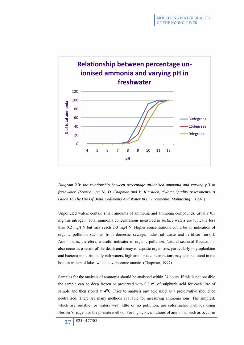
The change in percentage of the 2 forms at different pH values showing the relationship
between the percentages of un-ionised ammonia and varying pH in freshwater is shown in the
diagram that follows:
MODELLING WATER QUALITY OF THE NGONG’ RIVER
27 E25-0177/05
Diagram 2.3: the relationship between percentage un-ionised ammonia and varying pH in
freshwater. (Source: pg 78, D. Chapman and V. Kimstach, “Water Quality Assessments- A
Guide To The Use Of Biota, Sediments And Water In Environmental Monitoring”, 1997.)
Unpolluted waters contain small amounts of ammonia and ammonia compounds, usually 0.1
mg/l as nitrogen. Total ammonia concentrations measured in surface waters are typically less
than 0.2 mg/l N but may reach 2-3 mg/l N. Higher concentrations could be an indication of
organic pollution such as from domestic sewage, industrial waste and fertiliser run-off.
Ammonia is, therefore, a useful indicator of organic pollution. Natural seasonal fluctuations
also occur as a result of the death and decay of aquatic organisms, particularly phytoplankton
and bacteria in nutritionally rich waters, high ammonia concentrations may also be found in the
bottom waters of lakes which have become anoxic. (Chapman, 1997)
Samples for the analysis of ammonia should be analysed within 24 hours. If this is not possible
the sample can be deep frozen or preserved with 0.8 ml of sulphuric acid for each litre of
sample and then stored at 4⁰C. Prior to analysis any acid used as a preservative should be
neutralised. There are many methods available for measuring ammonia ions. The simplest,
which are suitable for waters with little or no pollution, are colorimetric methods using
Nessler’s reagent or the phenate method. For high concentrations of ammonia, such as occur in
0
20
40
60
80
100
120
4 5 6 7 8 9 10 11 12
% of total ammon
ia
pH
Relationship between percentage un‐ionised ammonia and varying pH in
freshwater
30degrees
15degrees
0degrees

MODELLING WATER QUALITY OF THE NGONG’ RIVER
28 E25-0177/05
wastewaters, a distillation and titration method is more appropriate. Total ammonia nitrogen is
also determined as part of the Kjedahl method (Ballance, 1996). This method of analysis is
described in the subsequent chapter.
2.6.1.2 Nitrate and Nitrite The nitrate ion is the common form of combined nitrogen found in natural waters. It may be
biochemically reduced to nitrite by denitrification processes, usually under anaerobic
conditions. The nitrite ion is rapidly oxidised to nitrate. Natural sources of nitrate to surface
waters include igneous rocks, land drainage and plant and animal debris. Nitrate is an essential
nutrient for aquatic plants and seasonal fluctuations of nitrates in water can be caused by plant
growth and decay. Natural concentrations, which seldom exceed 0.1 mg/l NO3—N, may be
enhanced by municipal and industrial wastewaters, including leachates from waste disposal
sites and sanitary landfills. In rural and suburban areas, the use of inorganic nitrate fertilisers
can be a significant source (D. Chapman, 1997).
When influenced by human activities, surface waters can have nitrate concentrations up to 5
mg/l NO3—N but often less than 1 mg/l NO3
—N. Concentrations in excess of 5mg/l NO3—N
usually indicate pollution by human and animal waste, or fertiliser run-off. In cases of extreme
pollution, concentrations may reach 200mg/l NO3—N. The World Health Organisation (WHO)
recommended maximum limit for NO3 in drinking water is 50 mg/l and waters with higher
concentrations can represent a significant health risk. (WHO 1984, Guidelines for drinking
water quality. Volume 2)
Nitrate occurs naturally in groundwater as a result of soil leaching but in areas of high nitrogen
fertiliser application it may reach very high concentrations (approximately 500 mg/l NO3—N).
In some areas, sharp concentrations in ground waters over the last 20 or 30 years have been
related to increased fertiliser applications (Hagebro et al., 1983; Roberts et al., 1987). Increased
fertiliser use is however not the only source of nitrate leaching into groundwater. Nitrate
leaching from unfertilised grassland or natural vegetation is normally minimal, although soils
in such areas contain sufficient organic matter to be a large potential source of nitrate. On
clearing and ploughing for cultivation, the increased soil aeration that occurs enhances the
action of nitrifying bacteria, and the production of soil nitrate.
Nitrite concentrations in freshwaters are usually very low, 0.001 mg/l NO2-N, are rarely higher
than 1 mg/l NO2-N. High nitrite concentrations are generally indicative of industrial effluent
and are often associated with unsatisfactory microbiological quality of water. (Hem, 1989).

MODELLING WATER QUALITY OF THE NGONG’ RIVER
29 E25-0177/05
Determination of nitrate plus nitrite in surface waters gives a general indication of the nutrient
status and level of organic pollution. Consequently, these specimens are included in most basic
water quality surveys and multipurpose or background monitoring programmes. As a result of
the potential health risk in high levels of nitrate, it is also measured in drinking water sources.
However, as little nitrate is removed during the normal processes for drinking water treatment.
Samples taken for the determination of nitrate and nitrite should be collected in glass or
polythene bottles and filtered and analysed immediately. If this is not possible, 2-4 ml of
chloroform per litre can be added to the sample to retard bacterial decomposition. The sample
can then be cooled and stored at 3-4 ⁰C. As determination of nitrate is difficult, due to
interferences from other substances present in the water, the precise choice of method may
vary according to the concentration of nitrate as N. Alternatively one sample can be analysed
for total nitrogen and the other for nitrite, and the nitrate concentration obtained from the
difference between the 2 values. Nitrite concentrations can be determined using
spectrophotometric methods. (Ballance, 1996).
2.6.1.3 Organic Nitrogen
Organic nitrogen consists mainly of protein substances (e.g. amino acids, nucleic acids and
urine) and the product of their biochemical decomposition transformations (e.g. humic acids
and fulvic acids). Organic nitrogen is naturally subject to the seasonal fluctuations of the
biological community because it is mainly formed in water by phytoplankton and bacteria, and
cycled within the food chain. Increased concentrations of organic nitrogen could be an
indication of pollution of the water body.
Organic nitrogen is usually determined using the Kjedahl method which gives total ammonia
nitrogen plus total organic nitrogen. The difference between the total nitrogen and the
inorganic forms gives the total organic nitrogen content. Samples must be unfiltered and
analysed within 24 hours, since organic nitrogen is rapidly converted to ammonia. This process
can be retarded if necessary by the addition of 2-4 ml of chloroform or 0.8 ml of concentrated
H2SO4 per litre of sample. Storage should be at 2-4 ⁰C, and when this is necessary, the
condition and duration of preservation should be stated with the results (Ballance et al., 1996).
Photochemical methods can also be used in place of Kjedahl method. These methods oxidise
all organic nitrogen (as well as ammonia) to nitrates and nitrites and, therefore, the
measurements of these must already have been carried out on the sample beforehand. If
samples are filtered total dissolved nitrogen is determined instead of the total organic nitrogen.

MODELLING WATER QUALITY OF THE NGONG’ RIVER
30 E25-0177/05
2.6.2 Phosphorus compounds
Phosphorus is an essential nutrient for living organisms and exists in water bodies as both
dissolved and particulate species. It is generally the limiting nutrient for algal growth and,
therefore, controls the primary productivity of a water body. Artificial increases in
concentrations due to human activities are the principal cause of eutrophication (Chapman,
1997).
In natural waters and in wastewaters, phosphorus occurs mostly as dissolved orthophosphates
and polyphosphates, and organically bound phosphates (Kimstach, 1997). Changes between
these forms occur continuously due to decomposition and synthesis of organically bound forms
of phosphate that occur at different pH values in pure water is shown in the diagram below:
Diagram 2.4: forms of phosphate that occur at different pH values in pure water. (Source:
page 85, D. Chapman and V. Kimstach, “Water Quality Assessments- A Guide To The Use Of
Biota, Sediments And Water In Environmental Monitoring”, 1997.)
It is recommended that phosphate concentrations are expressed as phosphorus, ie mg/l PO4-P
(and not as mg/l PO43-.
0
20
40
60
80
100
120
4 5 6 7 8 9 10 11 12
% of total pho
spha
tes
pH
Equilibrium of different forms of phosphates in relation to pH
H2PO4‐
HPO42‐
PO43‐
H2PO4‐
HPO4
MODELLING WATER QUALITY OF THE NGONG’ RIVER
31 E25-0177/05
Natural sources of phosphorus are mainly the weathering of phosphorus-bearing rocks and the
decomposition of organic matter (particularly those containing detergents), industrial effluents
and fertiliser run-off contribute to elevated levels in surface waters. Phosphorus associated with
organic and mineral constituents of sediments in water bodies can also be mobilised by
bacteria and released to the water column.
Phosphorus is rarely found in high concentrations in freshwaters as it is actively taken up by
plants. As a result there can be considerable seasonal fluctuations of phosphorus concentrations
in surface waters. In most natural surface waters, phosphorus ranges from 0.005 to 0.020 mg/l
PO4-P concentrations. As low as 0.001 mg/l PO4-P may be found in some enclosed saline
waters. Average groundwater levels are about 0.02 mg/l PO4-P (Hem, 1989).
High concentrations of phosphates can indicate the presence of pollution and are largely
responsible for eutrophic conditions.
Phosphorus concentrations are usually determined as orthophosphates, total inorganic
phosphate or total phosphorus (organically combined phosphorus and all phosphates). The
dissolved forms of phosphorus are measured after filtering the sample through a pre-washed
0.45 m pore diameter membrane filter. Particulate concentrations can be deduced by the
difference between total and dissolved concentrations. Phosphorus is readily absorbed onto the
surface of the sample containers and, therefore, containers should be rinsed thoroughly with the
sample before use. Samples for phosphate analysis can be preserved with chloroform and
stored at 2-4 ⁰C for up to 24 hours. Samples for total phosphorus determinations can be stored
in a glass flask with a tightly fitting glass stopper, provided 1 ml of 30% sulphuric acid is
added per 100 ml sample.
2.7 Results from previous studies and the gap that exists
A number of previous studies have been done to determine the quality of water of the Ngong
River. Among these, the most notable one is the Nairobi River Basin Project (NRBP) which
was initiated in 1999 to address pollution problems of the Nairobi Rivers. The Phase II of the
NRBP was conducted on the Ngong' /Motoine-Nairobi River to provide information and to
identify the major point sources of pollution. In the water quality assessment the longitudinal
profile of the Ngong' River was represented by 20 sample stations. The sample stations were as
shown in Table 2 that follows:

MODELLING WATER QUALITY OF THE NGONG’ RIVER
32 E25-0177/05
Table 2.1: station positions for NRDP UON/UNEP project (Feb. to Nov. 2003.)
STATION NUMBER STATION POSITION DISTANCE (km)
1 Motoine Dam 0.0
2 Ngong Rd bridge 2.5
3 Jamhuri Dam outlet 5.8
4 Ngong River 5.8
5 Kibera bridge 7.9
6 Inlet to Nairobi Dam 9.6
7 Midpoint of the dam 10.3
8 Weir 10.8
9 Langata Rd bridge 1 11.9
10 Langata Rd bridge 2 12.0
11 Mombasa Rd bridge 12.7
12 KCB bridge 14.2
13 Enterprise Rd bridge 15.1
14 Outer-ring rd bridge 17.8
15 Kangundo Rd bridge 25.4
16 Nairobi river confluence 27.1
17 Dandora sewage treatment
plant
28.7
18 After kamiti river confluence 32.3
19 After Nairobi falls 35.2
20 After ruiru confluence 42.3
In this current project, the scope of the study limits the section of the Ngong’ River to be
considered and the following sample stations were chosen:

MODELLING WATER QUALITY OF THE NGONG’ RIVER
33 E25-0177/05
Table 2.2: sampling stations selected for this experiment.
OLD STATION NUMBER NEW STATION
NUMBER
STATION POSITION
2 1 Ngong Rd bridge
3 2 Jamhuri Dam outlet
5 3 Kibera bridge
8 4 Weir
13 5 Enterprise Rd bridge
14 6 Outer-ring rd bridge
In order to facilitate a comparative analysis of the results obtained from assessment to the
pollution levels, the sample sites taken for this study coincide as far as possible with the
sampling stations for the Phase II of the NRBP, UoN-UNEP project. These include; Kariani
Dam on Ngong' Road, the outlet of Jamhuri park Dam, the Kibera bridge, the weir/outlet of
Nairobi Dam, Dunga Road bridge, and the outer ring road bridge.
The results from Phase II of the NRBP, UoN-UNEP project showed that the nutrients levels in
the Ngong River varied considerably. These results are shown in appendix 9.4.
At the upstream section, the concentration of phosphate was relatively low, but enough to
support excessive growth of the water plants at the stagnant sections of the river. The nitrite
levels were low varying from 0 to 0.3 mg/l. Ammonia concentration was also low at the
upstream section of the river, indicating absence of human waste contamination.
The ammonia concentration in the upstream was below 2 mg/l. However, the concentration
increased to 35 mg/l at the Kibera bridge. This was an indication of the presence of human
waste in the river. These high levels of ammonia was supported by the observation that several
toilets had been erected over the river. The free ammonia water was an indication of presence
of fresh sewage in the river. At the inlet to Nairobi dam, the ammonia concentration was 40
mg/l (NRDP- Phase II, UON/UNEP project, Feb- Nov 2003, Final report).
The water leaving the Nairobi dam showed free ammonia of 33mg/l. This was indication of
anoxic conditions. Wetlands are also major sources of ammonia arising from anaerobic
decomposition of organic matter. The concentration of free ammonia remained high at the
stations downstream, an indication of discharge of wastes high in free ammonia such as
domestic sewage and industrial discharges as well as existence of anoxic conditions in the
river. These would give rise to anaerobic breakdown of organic matter where ammonia is one
of the by-products. (NRDP- Phase II, UON/UNEP project, Feb- Nov 2003, Final report.)

MODELLING WATER QUALITY OF THE NGONG’ RIVER
34 E25-0177/05
During the wet weather, the free ammonia concentration in the river was 40 mg/l and below.
The cause of reduced levels of ammonia was dilution from surface runoff. However, whereas
ammonia concentration was low in the upstream stations averaging 0.4 mg/l, downstream, at
the industrial areas stations, the ammonia concentrations was between 26 – 28 mg/l. The major
source of free ammonia in the river was thus concluded to be due to discharge of human waste
mainly from the informal settlements (NRDP- Phase II, UON/UNEP project, Feb- Nov 2003,
Final report.)
The distribution of the nutrient pollutants were plotted into diagrams (appendix 9.3 and 9.4).
At the inlet of the Nairobi dam phosphate recorded a high of 2.5 mg/l, indicating contribution
from the Kibera informal settlement. Downstream of the Nairobi Dam up to the Mombasa
Road Bridge, phosphate concentration was between 0.1 mg/l and 0.2 mg/l, high enough to
cause high plant productivity in the river. Stations in the industrial area registered high levels
of phosphate of between 1.9 – 2.7 mg/l (NRDP- Phase II, UON/UNEP project, Feb- Nov 2003,
Final report.) The major source of phosphate pollution was taken to be from the informal
settlements, with other sources being industries.
The Final report from Phase II of the NRDP, UON/UNEP project, Feb- Nov 2003, thus
concluded that the natural sources of nutrient pollution included animal and human waste
sources. The animal sources include domestic waste in the form of compounds containing
nitrogen and phosphorus in free and combined form. The nitrogen and phosphorus combined in
waste products undergo decomposition to release nitrogen and phosphorus usually as oxides of
these elements. These oxides are subsequently sources of nutrients for plant growth.
The anthropogenic sources include surface run-off from agricultural land application and run-
off from factories producing or handling fertilizer products.
The excessive plant growth in the Ngong River also hinders flow of water resulting in stagnant
pools of water and reduced light transmittance and hence reduced dissolved oxygen exchange
from air to river water (NRDP- Phase II, UON/UNEP project, Feb- Nov 2003, Final report).
The management of organic pollution from domestic and industrial sources and farming
activities within the riparian way-leave will go a long way in reducing nutrients and hence
restoration of river ecological balanced flora and fauna.
Among the recommendations that were made in relation to the report, the following directly
address the presence of the nutrient pollutants in the Ngong River:

MODELLING WATER QUALITY OF THE NGONG’ RIVER
35 E25-0177/05
a) The discharge of human waste into the river should be addressed through efforts to
have human settlements and agricultural activities within the river relocated or
stopped.
b) The industrial discharges should be stopped through efforts by the industries to take
measures to address pollution emanating from their production processes.
c) Continue to build the capacity of the Local Authorities through improvement of the
monitoring laboratories and equipment as well as organizing refresher courses
Despite the strides made to analyse the water quality, there has been little attempt to model the
water quality of the Ngong' River as a support system tool for water pollution control as well as
the assessment of the effects of point and diffuse pollution.

MODELLING WATER QUALITY OF THE NGONG’ RIVER
36 E25-0177/05
3. RESEARCH METHODOLOGY The process of water quality modelling generally consists of the following steps (Himesh,
2000):
1. Orientation/ Problem identification
2. Formulation of relations between variables and parameters
3. Non dimensionalization
4. Solution of model equations
5. Preliminary test application
6. Model Verification
7. Reiteration of steps 2 – 6
8. Implementation
A modelling flow chart is shown in the diagram below:
Diagram 3.1: Modelling flow chart (adapted from Thomann and Mueller, 1987 and Chapra,
1997).

MODELLING WATER QUALITY OF THE NGONG’ RIVER
37 E25-0177/05
The steps are discussed below:
3.1 Orientation The modelling process always starts with an orientation stage, in which the modeller gets
aquainted with the system under consideration, that is, the Ngong' River. This is done by
means of observations and information from experts and literature. This stage also involves the
identification of the relevant variables and parameters that the system is meant to use to
interpret the system (Erturk et. al, 2004).
The variables include:
• the distance along the reach [L]= x
• the cross-section area [L2]= A(x)
• the flow rate along the reach [L3·T-1]= Q(x)
• the concentration of the relevant water quality variable [M·L-3]= C(x)
3.1.1 Data collection methods Data collection methods are the various techniques that are employed in order to carry out a
water quality assessment. They involve the measurement of the water discharge at the
sampling points as well as the collection and analysis of samples.
3.1.2 Measuring stream flow: The discharge is the volume flowing per unit period of time (Chapman, 1996).Discharge
should be measured at the time of sampling. An estimate method to determine discharge is to
measure the cross-sectional area of the stream and then getting a rough estimate of the velocity
of the river by measuring the time it takes a weighted float to travel fixed distance along the
stream.
For best results, the cross section of the stream at the point of measurement should have the
following ideal characteristics (Kuusisto, 1996):
• The velocities at all the points are parallel to one another and at right angles to the
cross section of the stream.
• The curves of distribution of velocity in the section are regular in the horizontal and
vertical planes
• The cross-section should be located at a point where the stream is nominally straight
for at least 50 m above and below the measuring station
• The velocities are greater than 10 to 15 cm/s
• The bed of the channel is regular and stable
MODELLING WATER QUALITY OF THE NGONG’ RIVER
38 E25-0177/05
• The depth of flow is greater than 30 cm
• The stream does not overflow its banks
• There is no aquatic growth in the channel
It is rare for all these characteristics to be present at any one measuring station and
compromises usually have to be made.
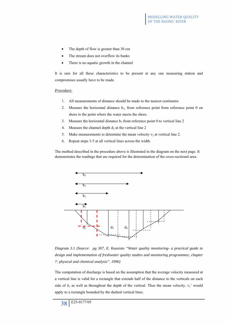
Procedure:
1. All measurements of distance should be made to the nearest centimetre
2. Measure the horizontal distance b1, from reference point from reference point 0 on
shore to the point where the water meets the shore.
3. Measure the horizontal distance b2 from reference point 0 to vertical line 2
4. Measure the channel depth d2 at the vertical line 2
5. Make measurements to determine the mean velocity v2 at vertical line 2.
6. Repeat steps 3-5 at all vertical lines across the width.
The method described in the procedure above is illustrated in the diagram on the next page. It demonstrates the readings that are required for the determination of the cross-sectional area.
b4
b3
b2
b1
d2 d3 d4
Diagram 3.1 (Source: pg 307, E. Kuusisto “Water quality monitoring- a practical guide to
design and implementation of freshwater quality studies and monitoring programmes; chapter
7: physical and chemical analysis”. 1996)
The computation of discharge is based on the assumption that the average velocity measured at
a vertical line is valid for a rectangle that extends half of the distance to the verticals on each
side of it, as well as throughout the depth of the vertical. Thus the mean velocity, v1’ would
apply to a rectangle bounded by the dashed vertical lines.

MODELLING WATER QUALITY OF THE NGONG’ RIVER
39 E25-0177/05
e.g. the area of a first rectangle is:
a1= *d2 Equation 3.1
Where: a1 = the area of the 1st rectangle of the cross-section
b2 = the horizontal distance to the 2nd point on the cross-section
d2 = depth of the river at the 2nd point of the cross-section
and the discharge through it will be:
Q1= a1*v1’ Equation 3.2
Where: v1’ = velocity of the river at the cross-section
The same procedure is repeated for the other rectangles. The discharge for the whole cross-
section will be:
Qt=Q1+Q2+......+QN = Qx Equation 3.3
Where: Qt = total discharge through the cross-section
Qx = discharge through each rectangle making up the cross-section area.
3.1.3 Sampling: Type of sampling that was employed in this study is grab sampling at selected depth and time.
Selection of sampling points is based on the following criteria (Ballance, 1996):
• To avoid polluted water at major outfalls such as drains, industrial outfalls, stagnant
pools and areas of standing water.
• To determine the effects of the dam and any standing water bodies along the stream
• Accessibility to sampling points.
• Cost effectiveness for collection, analysis and reporting
• To obtain spatially (along the profile of the river), hydrologically and temporally
distributed samples.
• Sustainability of the analysis system.
3.1.4 Materials and methods of water quality analysis For this particular study, the materials and methods that are considered are for the
determination of the nutrient pollution levels in the Ngong' River. Standard methods are used
for the analysis of nutrients.
MODELLING WATER QUALITY OF THE NGONG’ RIVER
40 E25-0177/05
3.1.4.1 BOD Standard methods were used to determine BOD. BOD is used as an approximate measure of
the amount of biochemically degradable organic matter present in a sample. The 5-day
incubation period has been accepted as the standard for this test (ISO 1990 – Water Quality).
BOD is useful for determining the relative waste loadings.
Sample handling
The test should be carried out as soon as possible after samples have been taken. If samples are
kept at room temperature for several hours, the BOD may change significantly, depending on
the character of the samples. Samples must be free from all added preservatives and stored in
glass bottles (Chapman D. 1997).
Interferences
If the pH of the sample is not between 6.5 and 8.5, add sufficient alkali or acid to bring it
within that range. Determine the amount of acid and alkali to be added by neutralising separate
portion of the sample to about pH 7.0 with 1 mol/l solution of the alkali or acid (Chapman D.
1997).
Apparatus
1. BOD bottles
2. Incubator
3. Beakers
4. pipette
Reagents
1. Phosphate buffer (dissolve 8.5g K2PO4, 21.75g K2HPO4, 33.4g Na2HPO4. 7H2O and
1.7g NH4Cl in 500ml of distilled water and dilute to 1 litre).
2. Magnesium sulphate solution (dissolve 22.5g Mg SO4.7H2O in distilled water and
dilute to 1 litre).
3. Calcium chloride solution (dissolve 27.5g CaCl2 in distilled water and dilute to 1
litre).
4. Ferric Chloride solution (dissolve 0.25g FeCl3.6H2O in distilled water and dilute to 1
litre)
Procedure
1. Into 1000ml distilled water, add 1 ml of each of the above reagents.
2. Aerate the above solution till the DO is at least 8mg/l.

MODELLING WATER QUALITY OF THE NGONG’ RIVER
41 E25-0177/05
3. Into a 250ml beaker, add the sample in 5, 10, 15 and 20ml amounts, making one as a
blank of only aerated water.
4. Make up to 200ml using the aerated water.
5. Measure the DO of each of the five solutions so made.
6. Transfer the solution above into the BOD bottle ensuring that there is no air trapped.
7. Cover with cellophane
8. Incubate at 20⁰ C for 5 days.
9. Measure the DO5.
Calculation
BOD, mg/l = Equation 3.4
Where:
D1 = DO of the diluted sample immediately after preparation, mg/l
D2 = DO of the diluted sample after 5 days incubation at 20⁰ C
P = decimal volumetric fraction of sample used.
3.1.4.2 Nitrogen ammonia: Palintest method was used to determine Nitrogen Ammonia. When nitrogen organic matter is
destroyed by microbiological activity, ammonia is produced and is therefore found in many
surface and ground waters. Higher concentrations occur in water polluted by sewage,
fertilisers, agricultural wastes or industrial wastes containing organic nitrogen, free ammonia or
ammonium salts (Ballance, 1997).
Certain aerobic bacteria convert ammonia into nitrites then nitrates. Nitrogen compounds, as
nutrients for aquatic micro-organisms, may be partially responsible for the eutrophication of
lakes and rivers. Ammonia can result from the natural reduction processes under anaerobic
conditions.
Sample handling
It is not possible to carry out the determination very soon after sampling, the sample should be
refrigerated at 4 degrees C. Chemical preservation may be achieved by adding either 20 -40 mg
HgCl2 or 1 ml H2SO4 to 1 litre of sample.

MODELLING WATER QUALITY OF THE NGONG’ RIVER
42 E25-0177/05
Principle
Ammonia can be quantitatively recovered from a sample by distillation under alkaline
conditions into a solution of boric acid followed by titration with standard acid. The method is
particularly suitable for the analysis of polluted surface water contain sufficient ammonia to
neutralise at least 1 ml of 0.00714 mol 1-1 HCl.
Apparatus
1. 1 litre round bottomed heat-resistant glass flask fitted with a splash head
2. Palintest Photometer at 640nm.
3. Usual laboratory glassware
Reagents
1. Palintest Ammonia No. 1 tablets.
2. Palintest Ammonia No. 2 tablets.
Procedure
1. Fill test tube with sample to the 10ml mark.
2. Add ammonia No. 1 and one ammonia No. 2 tablet, crush and mix to dissolve.
3. Stand for 10 minutes to allow colour development.
4. Select wavelength 640 nm on the photometer.
5. Take photometer reading (%T) in usual manner.
6. Consult ammonia calibration Diagram to find ammonia concentration.
Calculation
Ammonia nitrogen (as N) = ammonia reading in mg/1N.
The ammonia calibration table is shown below and is used for the determination of ammonia
concentration from the absorbance readings from the testing of the samples collected.
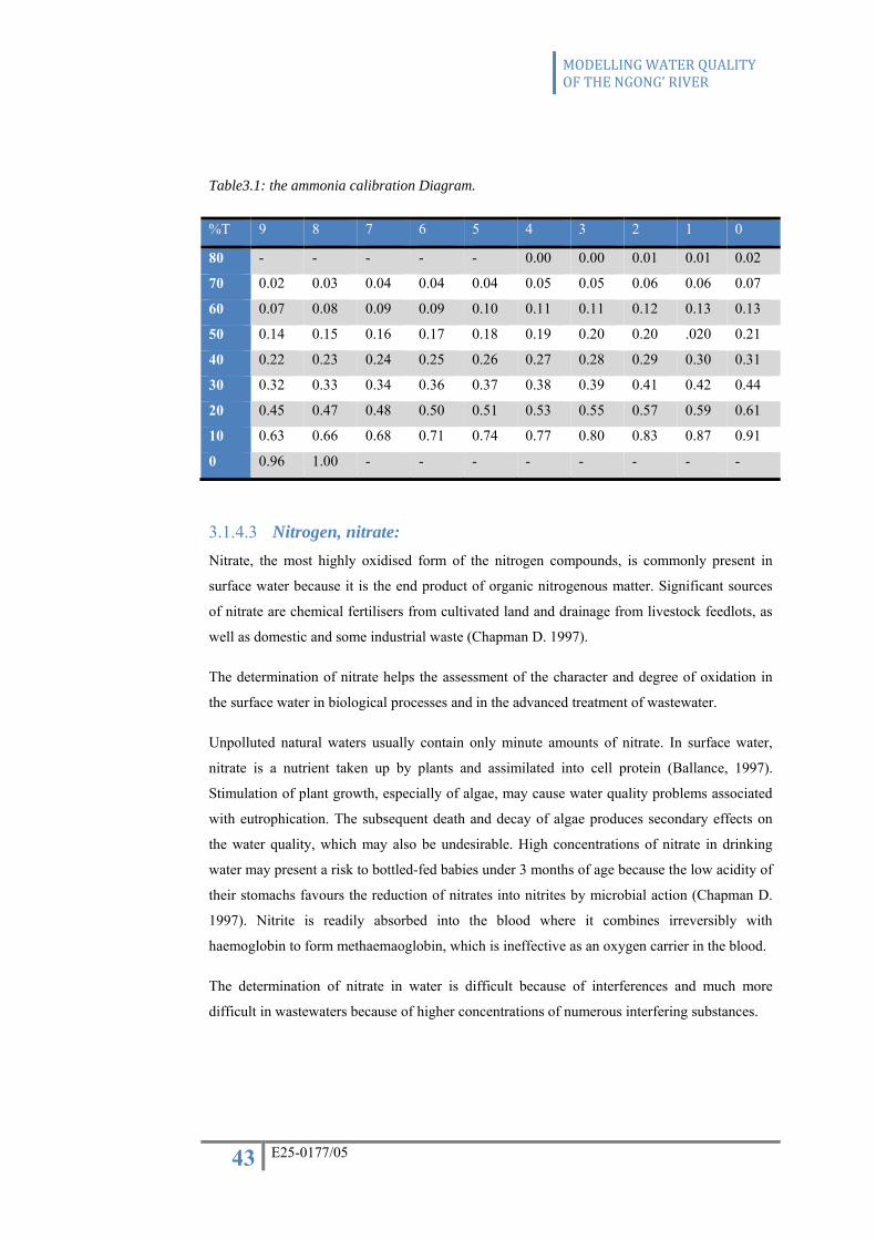
MODELLING WATER QUALITY OF THE NGONG’ RIVER
43 E25-0177/05
Table3.1: the ammonia calibration Diagram.
%T 9 8 7 6 5 4 3 2 1 0
80 - - - - - 0.00 0.00 0.01 0.01 0.02
70 0.02 0.03 0.04 0.04 0.04 0.05 0.05 0.06 0.06 0.07
60 0.07 0.08 0.09 0.09 0.10 0.11 0.11 0.12 0.13 0.13
50 0.14 0.15 0.16 0.17 0.18 0.19 0.20 0.20 .020 0.21
40 0.22 0.23 0.24 0.25 0.26 0.27 0.28 0.29 0.30 0.31
30 0.32 0.33 0.34 0.36 0.37 0.38 0.39 0.41 0.42 0.44
20 0.45 0.47 0.48 0.50 0.51 0.53 0.55 0.57 0.59 0.61
10 0.63 0.66 0.68 0.71 0.74 0.77 0.80 0.83 0.87 0.91
0 0.96 1.00 - - - - - - - -
3.1.4.3 Nitrogen, nitrate: Nitrate, the most highly oxidised form of the nitrogen compounds, is commonly present in
surface water because it is the end product of organic nitrogenous matter. Significant sources
of nitrate are chemical fertilisers from cultivated land and drainage from livestock feedlots, as
well as domestic and some industrial waste (Chapman D. 1997).
The determination of nitrate helps the assessment of the character and degree of oxidation in
the surface water in biological processes and in the advanced treatment of wastewater.
Unpolluted natural waters usually contain only minute amounts of nitrate. In surface water,
nitrate is a nutrient taken up by plants and assimilated into cell protein (Ballance, 1997).
Stimulation of plant growth, especially of algae, may cause water quality problems associated
with eutrophication. The subsequent death and decay of algae produces secondary effects on
the water quality, which may also be undesirable. High concentrations of nitrate in drinking
water may present a risk to bottled-fed babies under 3 months of age because the low acidity of
their stomachs favours the reduction of nitrates into nitrites by microbial action (Chapman D.
1997). Nitrite is readily absorbed into the blood where it combines irreversibly with
haemoglobin to form methaemaoglobin, which is ineffective as an oxygen carrier in the blood.
The determination of nitrate in water is difficult because of interferences and much more
difficult in wastewaters because of higher concentrations of numerous interfering substances.

MODELLING WATER QUALITY OF THE NGONG’ RIVER
44 E25-0177/05
Sample handling
To prevent any change in the nitrogen balance through biological activity, the nitrate
determination should be started as soon as possible after sampling. If storage is necessary,
samples should be kept at a temperature just above freezing point, with or without
preservatives, such as 0.8ml of concentrated sulphuric acid. If acid preservation is used then
the sample should be neutralised to about pH 7 immediately before the analysis is begun
(Chapman D. 1997).
The method used for the determination of nitrate level is the Phenol Disulphonic Acid method.
Principle
Nitrate in contact with sulphonic acid produces nitric acid which in dry condition (in presence
of excess concentrated H2SO4) brings about nitration of phenol disulphonic acid. This
nitrophenolic product gives intense yellow colour in alkaline medium which is measured
through colorimeter (the reaction must proceed in cold otherwise nitric acid may be lost by
volatization.)
Apparatus
1. Spectrometer
2. Hot water bath or similar apparatus
Reagents
1. Phenol disulphonic acid: dissolve 25 g of white phenol in 150 mL of concentrated
sulphuric acid then again add 85 mL of concentrated sulphuric acid. Heat it for 2 hrs
in a hot water bath, cool and keep the solution in a dark bottle.
2. Liquor ammonia(LR grade): it is diluted with equal volume of water.
3. Standard nitrate solutions: dissolve 0.722 g of anhydrous potassium nitrate in destilled
water to prepare 1 L of stock solution. This stock solution contains 100 mg NO3-N/L
(or 443 mg NO3 ions/L).
Procedure
1. Take 25 mL of sample in a porcelain dish (50 mL capacity) and evaporate it to
dryness on a hot water bath (if porcelain dish is not available take 50 mL beaker or
silica dish).
2. Add 3 mL of phenol disulphonic acid to the residue and dissolve the latter by rotating
the dish.

MODELLING WATER QUALITY OF THE NGONG’ RIVER
45 E25-0177/05
3. After 10 min, 15 mL of distilled water is added and stirred with a glass rod. On
cooling, the contents are washed down into 100 mL volumetric flask.
4. Add p. nitrophenal indicator
5. Add ammonia (1:1) slowly with mixing till the solution is alkaline as indicated by the
development of yellow color due to the presence of nitrate. Then add another 2 mL of
ammonia and the volume made up (100 mL) with distilled water.
6. Intensity of yellow colour is read in the colorimeter at 420nm (blue filter).
Observations
Preparation of standard curve for nitrate
A stock solution containing 100 ppm nitrate nitrogen (NO3-) is prepared by dissolving 0.7215 g
of AR grade potassium nitrate (oven-dried and cooled) in distilled water and making the
volume to one litre. This is diluted ten times to give a 10 ppm NO3- solution. Aliquots (2, 5,
10, 15, 20, 25 mL) are evaporated on boiling water bath to dryness in small porcelain dishes
(or beakers). When cool, 3 mL of phenol disulphonic acid is added and the yellow colour is
developed and read as described above. A blank (without nitrate) must be run and correction
made by adjusting the colorimeter to zero with blank. A calibration curve is drawn between
concentration of NO3- and colorimeter reading.
Calculation
Mg of NO3-/L =
Equation 3.5
3.1.4.4 Nitrogen, Nitrite Palintest method was used for the determination of nitrite concentration in the samples. Nitrite
is an unstable, intermediate stage in the nitrogen cycle and is formed in water either by the
oxidation of ammonia or by the reduction of nitrate (Ballance, 1997). Thus, biochemical
processes can cause a rapid change in the nitrite concentration in a water sample. In natural
waters nitrite is normally present only in low concentrations (a few tenths of an mg per litre).
Higher concentrations may be present in sewage and industrial wastes, in treated sewage
effluents and in polluted waters.
Sample handling
The determination should be made promptly on fresh samples to prevent bacterial conversion
of the nitrite to nitrate or ammonia. In no case should acid preservation be used for samples to

MODELLING WATER QUALITY OF THE NGONG’ RIVER
46 E25-0177/05
be analysed for nitrite. Short-term preservation for 1 to 2 days is possible by the addition of 40
mg mercuric ion as HgCl2 per litre of sample, with storage at 4⁰C (Ballance, 1997).
Interferences
There are very few known interferences as concentrations less than 1000 times that of nitrite.
However, the presence of strong oxidants or reductants in the samples will readily affect the
nitrite concentrations. High alkalinity (>600 mg/l as CaCo3) will give low results owing to a
shift in pH.
Apparatus
1. Palintest photometer
2. Round test tubes 10ml glass
Reagents
1. Palintest nitrocol tablets
Procedure
1. Fill round test tube with sample to the 10ml mark.
2. Add one nitrocol tablet, crush and mix to dissolve.
3. Select wavelength 520nm on the photometer.
4. Take photometer reading in usual manner
5. Consult nitrocol calibration Diagram to find nitrite concentration in the sample
The nitrocol calibration table for the determination of nitrite concentrations from the
absorbance of the sample is shown in the page that follows.

MODELLING WATER QUALITY OF THE NGONG’ RIVER
47 E25-0177/05
Table 3.3: nitrocol calibration Diagram for the determination of nitrite concentrations.
%T 9 8 7 6 5 4 3 2 1 0
90 0 .001 .003 .004 .006 .007 .009 .011 .012 .014
80 .016 .018 .019 .021 .023 .025 .027 .028 .030 .032
70 .034 .036 .038 .040 .042 .044 .046 .048 .051 .053
60 .055 .057 .060 .062 .064 .067 .069 .072 .074 .077
50 .079 .082 .084 .087 .090 .093 .096 .099 .102 .105
40 .108 .111 .114 .118 .121 .124 .128 .132 .135 .139
30 .143 .147 .151 .155 .160 .164 .169 .173 .178 .183
20 .189 .194 .200 .205 .212 .218 .224 .231 .238 .246
10 .254 .262 .271 .280 .290 .301 .312 .325 .338 .353
0 .369 .408 .431 .460 .5 - - - - -
Calculation
Read the concentrations of NO2-N in samples directly from the calibration curve. If less than
50 ml of the sample is taken, calculate the concentrations as follows:
Nitrite nitrogen (as N) =
mg/l Equation 3.6
3.1.4.5 Phosphates Phosphorus occurs in natural waters and wastewaters almost solely as phosphates. Phosphates
are presently in fertilisers and in many detergents. Consequently, they are carried into both
ground and surface waters with sewerage, industrial wastes and storm run-off (Ballance, 1997).
High concentrations of phosphorus compounds may produce a secondary problem in water
bodies where algal growth is normally limited by phosphorus. In such situations the presence
of additional phosphorus compounds can stimulate algal productivity and enhance
eutrophication processes.
Phosphates that respond to colorimetric tests without preliminary hydrolosis or oxidative
digestion of the sample are termed “reactive phosphorus.”
Principle
Organically combined phosphorus and all phosphates are first converted to orthophosphate. To
release phosphorus from combination with organic matter, a digestion or wet oxidation

MODELLING WATER QUALITY OF THE NGONG’ RIVER
48 E25-0177/05
technique is necessary. The least tedious method, wet oxidation with potassium
peroxydisulphate, is recommended.
Orthophosphate reacts with ammonium molybdate to form molybdophosphoric acid. This is
transformed by the reductants to the intensely coloured complex known as molybdenum blue.
The method based on reduction with ascorbic acid is preferable. Addition of potassium
antimonyl tartrate increases the coloration and the reaction velocity at room temperature.
For concentrations of phosphate below 20 g/l, the recommended procedure involves
extraction of the molybdenum blue complex from up to 200ml of water into a relatively small
volume of hexanol, so that a considerable increase in sensitivity is obtained.
Interferences
Relatively free from interferences. Arsenates react with the molybdate reagent to produce a
blue colour similar to that formed with phosphate. Concentrations as low as 0.1 mg As/L
interfere with the phosphorus determination. Hexavalent chromium and NO2- interfere to give
results about 3% low at concentrations of 1 mg/L and 10 to 15% low at 10 mg/L. Silfide (NaS)
and silicate do not interfere at concentrations of 1.0 and 10 mg/L.
Minimum detectable concentration is approximately 10 g P/L. P ranges as follows:
Approximately P range mg/L Light path (cm)
0.30-2.0 0.5
0.15-1.30 1.0
0.01-0.25 5.0
Apparatus
1. Colorimetric equipment: one of the following is required:
a. Spectrophotometer, with infrared phototube, for use at 880 nm, providing a
light path of 2.5 cm or longer.
b. Filter photometer equipped with a red colour filter and a light path of 0.5 cm
or longer
2. Acid washed glassware. Glassware should be left in sulphuric acid until required for
use.

MODELLING WATER QUALITY OF THE NGONG’ RIVER
49 E25-0177/05
Reagents
1. Sulphuric acid, H2SO4, 5N: dilute 70 mL of conc. H2SO4 to 500 mL with distilled
water
2. Potassium antimonyl tartrate solution: dissolve 1.3715 g K(SbO)C4H4O6. ½ H2o in
400 mL distilled water in a 500 mL volumetric flask and dilute to volume. Store in a
glass-stoppered bottle.
3. Ammonium molybdate solution: dissolve 20 g (NH4)6Mo7O24.4H2O in 500 mL of
distilled water. Store in a glass stoppered bottle.
4. Ascorbic acid, 0.1M: dissolve 1.76 g ascorbic acid in 100 mL distilled water. The
solution is stable for about 1 week at 4⁰C.
5. Combined reagent: mix the above reagents in the following proportions for 100 mL of
the combined reagent: 50 mL 5N H2SO4, 5 mL potassium antimonyl tartrate solution,
15 mL ammonium molybdate solution, and 30 ml ascorbic acid solution. Mix after
each addition of reagent. Let the reagents reach room temperature before they are
mixed and mix in the order provided. If the turbidity forms int he combined reagent,
shake and let stand for a few minutes until turbidity disappears before proceeding. The
reagent is stable for 4 hours.
6. Stock phosphate solution: dissolve in distilled water 219.5 mg anhydrous KH2PO4 and
dilute to 1000 mL; 1.00 mL = 50.0 g PO43- - P.
7. Standard phosphate solution: dilute 50.0 mL stock phosphate solution to 1000 mL
with distilled water; 1.00 mL = 2.50 g P
8. Phenolphthalein indicator solution. Dissolve 0.5g of phenolphthalein in 50ml of 95%
ethyl alcohol, and add 50 ml of distilled water. Add a dilute(e.g. 0.01 or 0.005 mol/l)
CO2 free solution of sodium hydroxide, a drop at a time, until the indicator turns
faintly pink.
Procedure
A. Treatment of sample
1. Pipet 50.0 mL of saple into a clean test tube or 125 mL flask.
2. Add 0.05 mL (1 drop) phenolphthalein indicator. If a red colour develops add 5N,
H2SO4 solution dropwise to just discharge the colour.
3. Add 8.0 mL combined reagent and mix thoroughly
4. After at least 10 min but no more than 30 min, measure absorbance of each sample at
880 nm, using reagent blank as the reference solution.

MODELLING WATER QUALITY OF THE NGONG’ RIVER
50 E25-0177/05
B. Correction for turbidity or interfering colour
5. Natural colour of water generally doesn’t interfere at the high wavelength used. For
highly coloured or turbid waters, prepare a blank by adding all the reagents except
ascorbic acid and potassium antimonyl tartrate to the sample. Subtract blank
absorbance of each sample.
C. Preparation of calibration curve
6. Prepare individual calibration curves from the series of 6 standards. Use a distilled
water blank with combined reagent to make the photometric readings for the
calibration curve.
7. Plot absorbance versus phosphate concentration to give a straight line passing through
the origin.
8. Test at least 1 phosphate standard with each sample.
Calculation
mg P/L =
Equation 3.7
3.2 Formulation of relations between variables and parameters The next step is to formulate relations between variables and parameters. For certain classes of
systems these relations have been established already long ago. Consistency is important. This
involves fixing functions to data. For the purpose of this study linear functions and intrinsically
linear functions will be used.
The term ‘linear’ in linear regression means that the function is a linear combination of basis
functions. With the basis function {1,x}, linear functions are those that can be written in the
form:
y= β0 + β1x Equation 3.8
while ‘intrinsically linear functions are those functions that can be written in the form:
y= β0f0 + β1f1 + β2f2 + β3f3 + .... + βnfn Equation 3.9
where βi are constants and the fi are the basis functions.
3.3 Non-dimensionalization This is the partial and full removal of units from an equation involving physical quantities by a
suitable substitution of variables. This technique can simplify and parametrize problems where

MODELLING WATER QUALITY OF THE NGONG’ RIVER
51 E25-0177/05
measured units are involved. It is closely related to dimensional analysis. To non-
dimensionalize a system the following steps are taken:
1. Identify all the independent and dependent variables.
2. Replace each of them with a quantity scaled relative to a characteristic unit of measure
to be determined.
3. Divide through by the co-efficient of the highest order polynomial or derivative term.
4. Choose judiciously the definition of the characteristic unit for each variable so that the
coefficients of as many as possible become 1.
5. Rewrite the system of equations in terms of their new dimensionless quantities.
3.4 Solution of model equations Since most models are in the first instance not tractable, it is good policy to solve the model
equations before preliminary test application. The stage involves the search for mathematical
solutions.
3.5 Preliminary test application Depending on the water quality variable, the analytical solution of this equation may be simple
or complex and even impossible for some cases. The distributed source terms (especially
distributed loads with flow) make the analytical solution very complex or even impossible,
when several water quality variables that depend on each other have to be expressed in form of
a system of differential equations.
3.6 Model Verification It is the testing of the calibrated model against the additional set of field data preferably under
different environmental conditions (river flow, waste load etc.), to further examine the range of
validity of the calibrated model. Collection of data for validation is such that, calibration
parameters are fully independent of the validation data. The model so verified can be used for
forecasting of water quality under a variety of perturbed environmental conditions. If a
numerical way has been found to solve the model, it remains to explore the solution as a
function of the independent variables and the adjustable parameters.
3.7 Reiteration of steps 2-6 After comparing the measured data and the calculated solution, one can improve on the model
and this is done by repeating steps 2-6. In view of the iteration process, it is convenient to
follow a modular approach from the beginning.

MODELLING WATER QUALITY OF THE NGONG’ RIVER
52 E25-0177/05
3.8 Implementation If the model suffices then it is implemented. This means that the results can be used by non
mathematicians. The appropriate presentation of the results is an important part of the
implementation process.
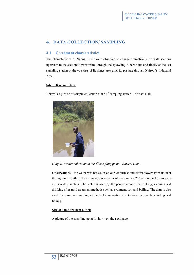
MODELLING WATER QUALITY OF THE NGONG’ RIVER
53 E25-0177/05
4. DATA COLLECTION/ SAMPLING
4.1 Catchment characteristics The characteristics of Ngong' River were observed to change dramatically from its sections
upstream to the sections downstream, through the sprawling Kibera slum and finally at the last
sampling station at the outskirts of Easlands area after its passage through Nairobi’s Industrial
Area.
Site 1: Kariaini Dam:
Below is a picture of sample collection at the 1st sampling station – Kariani Dam.
Diag 4.1: water collection at the 1st sampling point – Kariani Dam.
Observations - the water was brown in colour, odourless and flows slowly from its inlet
through to its outlet. The estimated dimensions of the dam are 225 m long and 30 m wide
at its widest section. The water is used by the people around for cooking, cleaning and
drinking after mild treatment methods such as sedimentation and boiling. The dam is also
used by some surrounding residents for recreational activities such as boat riding and
fishing.
Site 2: Jamhuri Dam outlet:
A picture of the sampling point is shown on the next page.

MODELLING WATER QUALITY OF THE NGONG’ RIVER
54 E25-0177/05
Water that flows from this point is clear and odourless.
Diag 4.2: the water that flows out of Jamhuri grounds to then flow into Kibera.
Observations – the area around is heavily polluted with human waste, plastic bags, rotten
food, rags, broken bottles and other rubbish. The water from the exit point out of Jamhuri
Park is however clear as if flows into the river. The water flows at a moderate rate. The
section of the river at this point is about 0.3 m long and 0.2 m at its deepest section.
Beyond this point there are many dumpsites and the water becomes brackish at the point
where the river flows under the bridge seperating Jamhuri and Kibera. The area has no
visible sewerage network and open sewers are seen to plainly discharge their material
straight into the river.
A picture of Ngong' River as it flows below the bridge separating Jamhuri from Kibera is
shown in the next page.

MODELLING WATER QUALITY OF THE NGONG’ RIVER
55 E25-0177/05
Diag 4.3: the river as it flows from the bridge separating Jamhuri and Kibera.
Site 3: Kibera bridge:
A picture of the process of sample collection at the Kibera Bridge is shown in the picture
below:
Diag 4.4: the Ngong' River as it passes through Kibera.
Observations – this is visibly one of the most polluted sections of the river. The water is
brackish and polluted with sediments from the surface runoff along the embankments of
the river and the discharge of raw sewage directly into the river. The water has a foul
odour and has a sluggish flow. Open sewers discharge their wastewater directly into the
river. The area is surrounded by dumpsites containing plastic bags, rotten food, rags,
broken bottles and other rubbish.
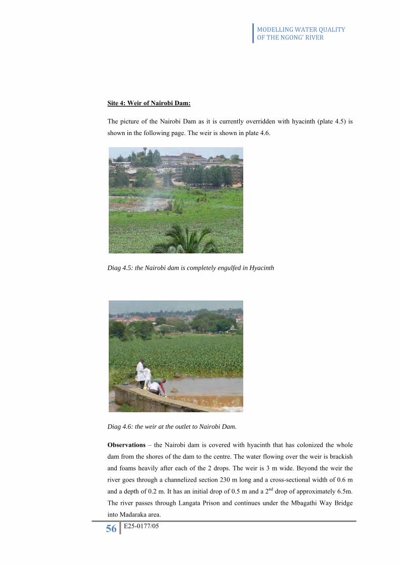
MODELLING WATER QUALITY OF THE NGONG’ RIVER
56 E25-0177/05
Site 4: Weir of Nairobi Dam:
The picture of the Nairobi Dam as it is currently overridden with hyacinth (plate 4.5) is
shown in the following page. The weir is shown in plate 4.6.
Diag 4.5: the Nairobi dam is completely engulfed in Hyacinth
Diag 4.6: the weir at the outlet to Nairobi Dam.
Observations – the Nairobi dam is covered with hyacinth that has colonized the whole
dam from the shores of the dam to the centre. The water flowing over the weir is brackish
and foams heavily after each of the 2 drops. The weir is 3 m wide. Beyond the weir the
river goes through a channelized section 230 m long and a cross-sectional width of 0.6 m
and a depth of 0.2 m. It has an initial drop of 0.5 m and a 2nd drop of approximately 6.5m.
The river passes through Langata Prison and continues under the Mbagathi Way Bridge
into Madaraka area.

MODELLING WATER QUALITY OF THE NGONG’ RIVER
57 E25-0177/05
Site 5: Dunga Rd bridge:
A picture of the sample collection process at the 5th sampling station at the Dunga Road
Bridge is shown below:
Diag 4.7: the channelized section of Ngong' River as it flows through the industrial area.
Observations –this sampling point is next to Mater Hospital. This section of Ngong' River
is channelized as it passes through Industrial Area. The channel is 4.0 m wide and 0.6 m
deep. The water is brackish and slow moving. The embankments are littered with garbage
– plastic paper bags, sacks, cloths.
Site 6: Outer-ring Rd Bridge:
The level of pollution in the Ngong' River at the Outer-ring Road bridge is shown in plate
4.8 below.
Diag 4.8: water flowing under the bridge on Outer-ring road.

MODELLING WATER QUALITY OF THE NGONG’ RIVER
58 E25-0177/05
Observations –the water appears to be heavily polluted. The water is black in colour and
has a foul smell. The embankments are littered with garbage- plastic bags, rags, broken
bottles and other rubbish. The river is slow moving with some areas being wider than
others due to dumping of waste into the river and sedimentation of soil due to the decrease
in flow rate. At the sampling point the river was 2.5 m wide.

MODELLING WATER QUALITY OF THE NGONG’ RIVER
59 E25-0177/05
5. SAMPLE RESULTS AND DATA ANALYSIS
5.1 Longitudinal Profile The altitudes of the various sampling points and the distance between them were obtained from
previous studies carried out by NRBP- Phase II and NEMA reports. The data collected from
this desk study is shown in Table 5.1 below.
Table 5.1: longitudinal profile of the Ngong' River
SAMPLE
STATION NO.
NAME HASL (M) DISTANCE
(KM)
SLOPE OF
BED = i
1 Kariani Dam 1920 0.0 -
2 Jamhuri Dam
outlet
1850 3.3 0.0212
3 Kibera bridge 1790 5.4 0.0286
4 Weir of Nairobi
dam
1690 8.3 0.0345
5 Dunga Rd
Bridge
1660 12.6 0.0070
6 Outer-ring Rd 1610 15.3 0.0185
The longitudinal profile is plotted in the diagram below that shows the height above sea level
at the various sampling stations.
Diagram 5.1: longitudinal profile of the Ngong' River.
1920
1850
1790
16901660
1610
14501500155016001650170017501800185019001950
0 3.3 5.4 8.3 12.6 15.3
HEIGHT ABO
VE SEA LEV
EL
DISTANCE ALONG THE PROFILE (km)
LONGITUDINAL PROFILE
LONGITUDINAL PROFILE

MODELLING WATER QUALITY OF THE NGONG’ RIVER
60 E25-0177/05
5.2 Cross-sectional Profile The cross-sectional properties at the various sampling stations is summarised in the table below.
Table 5.2: sampling stations and cross-sectional properties
sample
station
Name W (m) D(m) A(m2) P (m) SHAPE z= (y/x)
1 Kariani
Dam
30.00 2.30 63.71 31.91 sym
trapezoid
1.0
2 Jamhuri
Dam
outlet
0.30 0.20 0.04 0.55 sym
trapezoid
2.0
3 Kibera
bridge
2.00 0.50 0.75 1.71 sym
trapezoid
1.0
4 Weir of
Nairobi
dam
0.60 0.20 0.12 1.00 sym
rectangle
-
5 Dunga Rd 4.00 0.60 2.4 5.20 sym
rectangle
-
6 Outer-
ring Rd
2.50 0.70 1.26 3.08 sym
trapezoid
1.0
Where:
W = width of the river at the sampling station
D= depth of the river at the sampling station
A= cross-sectional area of river at the sampling station
z= slope of the sides of the embankments.
5.3 Biochemical Oxygen Demand The results from the experiments to determine the BOD5 for the water samples taken are given
in table 5.3 in the page that follows. Also given are the average BOD5 values from the different
rounds of sampling.

MODELLING WATER QUALITY OF THE NGONG’ RIVER
61 E25-0177/05
Table 5.3: results of BOD tests
SAMPLE
STATION
ROUND 1
(19.09.10)
ROUND 2
(26.09.10)
ROUND 3
(10.10.10)
ROUND 4
(17.10.10)
AVE BOD5
1 73.22 65.41 69.22 63.06 67.72
2 55.17 53.53 59.37 65.37 58.36
3 146.00 147.33 141.91 153.39 147.16
4 134.67 137.25 141.91 131.37 136.30
5 282.35 285.15 293.07 321.57 295.53
6 313.73 320.00 328.00 356.44 329.54
The BOD value at station 1 is 67.72 mg/L. This decreases to 58.36mg/L at station 2. The
decrease could be attributed to self purification of the river at the Jamhuri Dam. The BOD
increases to 147.16 mg/L at station 3 – Kibera Bridge. The increase in BOD could be attributed
to the disposal of raw human waste and other organic rubbish directly into the river. When
these decompose, they use up oxygen from the river resulting in a high BOD value. The BOD
reduces to 136.30 mg/L at station 4 – weir at outlet of Nairobi Dam. This reduction in BOD
could be attributed to the fact that Nairobi Dam acts as a stabilising pond of the Ngong' River
as it flows out of Kibera slum. The BOD increases to 295.53 mg/L at station 5- Dunga Road
Bridge. By the time the river has reached this point, it has passed close to informal settlements,
pharmaceutical, inks, dyes, edible oils and flour companies. The BOD level is highest at station
6 – on Outering Road bridge. It is understandable that this would register the highest BOD
levels because by this point the river has passed through the Eastlands area that is characterised
by numerous abattoirs, car-washes, human settlements and industries. It is also victim to being
used as a garbage disposal site as is evident at the sampling station.
The BOD5 from the different sampling stations is shown in the diagram on the next page in
diagram 5.3a and the average line graph shown in diagram 5.3b.
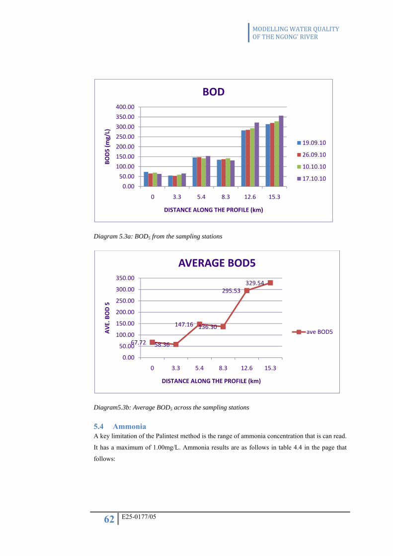
MODELLING WATER QUALITY OF THE NGONG’ RIVER
62 E25-0177/05
Diagram 5.3a: BOD5 from the sampling stations
Diagram5.3b: Average BOD5 across the sampling stations
5.4 Ammonia A key limitation of the Palintest method is the range of ammonia concentration that is can read.
It has a maximum of 1.00mg/L. Ammonia results are as follows in table 4.4 in the page that
follows:
0.00
50.00
100.00
150.00
200.00
250.00
300.00
350.00
400.00
0 3.3 5.4 8.3 12.6 15.3
BOD5 (m
g/L)
DISTANCE ALONG THE PROFILE (km)
BOD
19.09.10
26.09.10
10.10.10
17.10.10
67.72 58.36
147.16 136.30
295.53329.54
0.00
50.00
100.00
150.00
200.00
250.00
300.00
350.00
0 3.3 5.4 8.3 12.6 15.3
AVE. BOD 5
DISTANCE ALONG THE PROFILE (km)
AVERAGE BOD5
ave BOD5

MODELLING WATER QUALITY OF THE NGONG’ RIVER
63 E25-0177/05
Table 5.3: results from ammonia testing at the sampling stations
SAMPLE
STATION
19.09.10 26.09.10 10.10.10 17.10.10 ave ammonia reading
mg/L N
1 0.06 0.06 0.05 0.11 0.07
2 0.01 0.01 0.02 0.04 0.02
3 1.00 1.00 1.00 1.00 1.00
4 1.00 1.00 1.00 1.00 1.00
5 1.00 1.00 1.00 1.00 1.00
6 1.00 1.00 1.00 1.00 1.00
Ammonia usually originates from specific industrial discharges and human waste such as urine
or from anaerobic decomposition of organic matter. It is highly toxic to fish and other aquatic
animals in concentrations greater than 5 mg/L. The ammonia levels at samples stations 1 and 2
are low indicative of the fact that the river at these 2 points is relatively free of human waste
pollution. However, there is an escalation in level of ammonia from sample stations 3 to 6.
This is indicative of heavy human waste pollution. It was observed especially that in the Kibera
slum there were toilets that were erected over the river or which visibly discharged their waste
material into the river.
The ammonia concentration is shown in the diagrams that follow:
Diagram 5.4a: Ammonia values from the sampling stations
0.00
0.20
0.40
0.60
0.80
1.00
1.20
0 3.3 5.4 8.3 12.6 15.3
AMMONIA (m
g/L)
DISTANCE ALONG THE PROFILE (km)
AMMONIA
19.09.10
26.09.10
10.10.10
17.10.10

MODELLING WATER QUALITY OF THE NGONG’ RIVER
64 E25-0177/05
The water sample taken from the weir at the outlet of Nairobi also demonstrated high levels of
ammonia. From previous study, it can be shown that this could be due to anoxic conditions
present is the dam. This is because wetlands are a major source of ammonia arising from
anaerobic decomposition of organic matter. The concentrations of free ammonia further on
downstream was further indication of discharge of domestic sewage and industrial waste as
well as existence of anoxic conditions in the river. These would arise to anaerobic breakdown
of organic matter where ammonia is one of the by-products.
Diagram 5.4b: Average ammonia values from the sampling stations
5.5 Nitrite Results from the samples for the presence of nitrite are given in the table that follows.
0.07 0.02
1.00 0.95 1.00 1.00
0.00
0.20
0.40
0.60
0.80
1.00
1.20
0 3.3 5.4 8.3 12.6 15.3
AVE AMMONIA (m
g/L)
DISTANCE ALONG THE PROFILE (km)
ave ammonia
ave ammonia

MODELLING WATER QUALITY OF THE NGONG’ RIVER
65 E25-0177/05
Table 5.5: results from the nitrite testing from the sampling stations
SAMPLE
STATION
19.09.10 26.09.10 10.10.10 17.10.10 ave
NITRITE
(mg/L)
1 0.05 0.05 0.05 0.10 0.06
2 0.05 0.05 0.05 0.10 0.06
3 0.45 0.45 0.45 0.40 0.44
4 0.1 0.1 0.1 0.10 0.10
5 0.15 0.15 0.15 0.15 0.15
6 0.2 0.2 0.2 0.30 0.23
The nitrite concentration in the river is relatively low throughout the profile of the river and is
indicative of the relative low presence of nitrites. Most nitrogenous material in natural water
sources tend to be converted into nitrates, so nitrites should be considered as potential sources
of organic nitrates. Nitrites are also consumed by plants and other organisms. Major industries
that contribute to nitrite concentration in water sources include – nitrogenous fertilizer,
miscellaneous industrial inorganics, fertilizer mixing, explosives and canned foods. Nitrite
concentrations can be increased by the biochemical reduction of nitrates by denitrification
processes, usually under anaerobic conditions.
Nitrite concentration in the sampling stations upstream was lower than for sampling stations
downstream. The concentration rose to 0.44 mg/L at sampling station 3 – Kibera Slum. This
was indicative of inflow of human waste into the river. The concentration of nitrite decreased
to 0.1 mg/L at the weir of Nairobi Dam. This reduction in concentration of nitrite is attributed
to consumption by the hyacinth weed that has colonised the dam. The concentration increased
slightly to 0.15 mg/L at the Dunga Rd bridge sampling station and then rose to 0.23 mg/L at
the Outering Rd bridge sampling station. This increase would be attributed to further pollution
from the industries in Industrial area that discharge their effluent into the river as well as the
product of human waste being disposed into the river due to the informal settlements along the
bank.
The nitrite concentration at the various sampling stations is shown in the diagrams that follow.

MODELLING WATER QUALITY OF THE NGONG’ RIVER
66 E25-0177/05
Diagram 5.5a: Nitrite results from the sampling stations
The average nitrite concentration gotten from the mean of the sampling done is shown in
diagram 5.5b below.
Diagram 5.4b: average nitrite results from the sampling stations
5.6 Nitrates The determination of nitrates involves the preparation of a stock solution and the plotting of the nitrates to absorbance diagram to facilitate the determination of the concentrations of nitrates from samples collected. The standard graph is found in the following page.
00.050.1
0.150.2
0.250.3
0.350.4
0.450.5
0 3.3 5.4 8.3 12.6 15.3
NITRITE
(mg/L)
DISTANCE ALONG THE PROFILE (km)
NITRITE
19.09.10
26.09.10
10.10.10
17.10.10
0.06 0.06
0.44
0.100.15
0.23
0.000.050.100.150.200.250.300.350.400.450.50
0 3.3 5.4 8.3 12.6 15.3
AVE. NITRITE
(mg/L)
DISTANCE ALONG THE PROFILE (km)
ave NITRITE (mg/L)
ave NITRITE (mg/L)

MODELLING WATER QUALITY OF THE NGONG’ RIVER
67 E25-0177/05
Diagram 5.6a: standard solution line
The table that follows gives the results from the test for nitrates in the samples taken from the river.
Table 5.6: results from the tests done on the samples from the sampling stations
sample
station
19.09.10 26.09.10 10.10.10 17.10.10 ave NITRATES (mg
NO3-/L)
1 30.00 32.00 40.00 20.00 30.50
2 60.00 40.00 50.00 32.00 45.50
3 20.00 40.00 60.00 20.00 35.00
4 20.00 40.00 40.00 20.00 30.00
5 100.00 120.00 100.00 120.00 110.00
6 70.00 40.00 20.00 28.00 39.50
Nitrate concentrations in excess of 5 mg/L usually indicate pollution by human or animal
waste, or fertiliser run-off. In cases of extreme pollution, concentrations may reach 200 mg/L.
The WHO has recommended that the maximum nitrate concentration for water for human
consumption should not exceed 50 mg/L as waters with high concentration can exhibit a high
health risk.
y = 0.0393x + 0.0257
0.00
0.20
0.40
0.60
0.80
1.00
1.20
1.40
1.60
1.80
0 10 20 30 40 50
ABS
NITRATES (ml)
NITRATES
Series2
Linear (Series2)

MODELLING WATER QUALITY OF THE NGONG’ RIVER
68 E25-0177/05
The nitrate concentration at sampling station 1 – Kariani dam was 30.50 mg/L and this
increased to 45.5 mg/L at sampling station 2 – Jamhuri Dam outlet. The concentration then
reduced to 35.00 mg/L at the Kibera bridge sampling station. This reduction in nitrate
concentration could be attributed to anaerobic conditions present in the river at this point
preventing the oxidation of nitrogenous material. The nitrate concentration decreases further to
30.0 mg/L at the weir of Nairobi dam. This may be due to uptake by the hyacinth that has
colonised the dam. The nitrate concentration at sampling station 5 is the highest recorded from
all the sampling stations at an average nitrate concentration of 110 mg/L. This reduces to 39.5
mg/L at the last sampling station.
The results have been plotted and appear on the graph below.
Diagram 5.6b: Nitrate results from the sampling stations
0.00
20.00
40.00
60.00
80.00
100.00
120.00
140.00
0 3.3 5.4 8.3 12.6 15.3
NITRA
TES (m
g/L)
DISTANCE ALONG THE PROFILE (km)
NITRATE
19.09.10
26.09.10
10.10.10
17.10.10

MODELLING WATER QUALITY OF THE NGONG’ RIVER
69 E25-0177/05
Diagram 5.6c: average Nitrate results from the sampling stations
5.7 Phosphates The determination of phosphates involves the preparation of a stock solution and the plotting of the phosphate to absorbance diagram to facilitate the determination of the concentrations of phosphates from samples collected. The standard graph is found in the following page.
Diagram 5.7a: the standard concentration phosphates diagram.
30.50
45.5035.00 30.00
110.00
39.50
0.00
20.00
40.00
60.00
80.00
100.00
120.00
0 3.3 5.4 8.3 12.6 15.3
ave NITRA
TES (m
g/L)
DISTANCE ALONG THE PROFILE (km)
ave NITRATES (mg NO3‐/L)
ave NITRATES (mg NO3‐/L)
y = 0.0294x ‐ 0.0372
0.00
0.20
0.40
0.60
0.80
1.00
1.20
1.40
1.60
0 20 40 60
ABS
PHOSPHATES (ml)
PHOSPHATES
Series1
Linear (Series1)
MODELLING WATER QUALITY OF THE NGONG’ RIVER
70 E25-0177/05
The results from the tests done to determine the phosphates concentrations are shown in the table that follows:
Table 5.7: phosphate results from the tests done on the samples from the sampling stations
sample
station
19.09.10 26.09.10 10.10.10 17.10.10 ave PHOSPHATES
(mg/L)
1 0.00 0.00 0.00 0.00 0.00
2 0.00 0.00 0.00 0.00 0.00
3 0.91 1.10 0.96 1.03 1.00
4 0.65 0.72 0.55 0.50 0.60
5 0.62 0.77 0.55 0.58 0.63
6 1.01 1.03 0.99 0.84 0.97
There can be considerable fluctuations in phosphate concentrations in surface waters.
Phosphates are rarely found in high concentrations in fresh waters as it is actively taken up by
plants (Chapman D. et al, 1997). The concentrations of phosphates in sampling stations
upstream, registered absence of phosphates with an average of 0.00 mg/L from samples taken
at the different sampling times. The highest concentration of phosphates in the Ngong' River
was found at sampling station 3 – Kibera slum, where the concentration was 1.00 mg/L. This is
indicative of presence of pollution from domestic wastewaters, especially those containing
detergents and industrial effluents. The concentration decreases to 0.60 mg/L at the weir of
Nairobi dam. This reduction could be attributed to active uptake of phosphates by the hyacinth
present on the surface water of the Nairobi Dam. The phosphate concentration at sampling
station 5 is relatively the same as the for the previous station with a difference of 0.03 mg/L.
The concentration goes up to 0.97 mg/L at the Outer-ring Rd bridge (sampling station 6),
which can be attributed to pollution from the industries in the Industrial area of Nairobi and
numerous car washes and motor vehicle garages that discharge their effluent into the Ngong'
River.
The results are plotted and shown in the following diagrams; 4.7a and 4.7b.

MODELLING WATER QUALITY OF THE NGONG’ RIVER
71 E25-0177/05
Diagram 5.7b: Phosphate results from the sampling stations
Diagram 5.7c: Average Phosphate results from the sampling stations
5.8 Comparison of results from 2003 with 2010 From the initial base data obtained by the Nairobi River Basin Project –Phase II carried out in
2003, the following data is available for the preparation of the model awaiting further
calibration using present day results. These results are shown in the table on the next page:
0.00
0.20
0.40
0.60
0.80
1.00
1.20
0 3.3 5.4 8.3 12.6 15.3
PHOSPHATES (m
g/L)
DISTANCE ALONG THE PROFILE (km)
PHOSPHATES
19.09.10
26.09.10
10.10.10
17.10.10
0.00 0.00
1.00
0.60 0.63
0.97
0.00
0.20
0.40
0.60
0.80
1.00
1.20
0 3.3 5.4 8.3 12.6 15.3
ave PH
OSPHATES (m
g/L)
DISTANCE ALONG THE PROFILE (km)
ave PHOSPHATES (mg/L)
ave PHOSPHATES (mg/L)

MODELLING WATER QUALITY OF THE NGONG’ RIVER
72 E25-0177/05
Table 5.8: results from the NRBP- Phase II, for BOD and nutrients.
Base station BOD5 (mg/l) NH4-N
(mg/l)
NO3-N
(mg/l)
NO2-N
(mg/l)
PO4-P
(mg/l)
Kariani Dam
(2)
73.00 1.40 - 0.00 0.10
Jamhuri
Dam outlet
(3)
35.00 1.60 - 0.02 0.14
Kibera
bridge (5)
147.50 35.00 - 0.00 0.33
Weir of
Nairobi Dam
(8)
64.00 33.00 - 0.01 0.32
Enterprise
Rd bridge
(13)
370.00 39.00 - 0.07 2.91
Outerring
Rd bridge
(14)
403.00 33.00 - 0.01 2.03
There are no comparable results for nitrate tests. These results from 2003 are compared with
the results from testing in 2010 and are shown in the diagrams 5.8 to 5.12.

MODELLING WATER QUALITY OF THE NGONG’ RIVER
73 E25-0177/05
Diagram 5.8: comparison of BOD in 2003 versus 2010
It can be concluded that the BOD levels are generally the same when compared between 2003
and 2010. This implies that pollution levels have remained constant over time.
Diagram 5.9: comparison of nitrite in 2003 versus 2010
The nitrite levels are conspicuously lower in 2003 than in 2010. The difference in nitrite levels
could be due to a number of reasons:
• Different testing methods between NRBP Phase II and the current method
• An increase in nitrite pollution in 2010 when compared to 2003.
0
100
200
300
400
500
0 2 4 6 8
BOD (m
g/L)
SAMPLE STATIONS
COMPARISON OF BOD IN 2003 VS 2010
BOD (2003)
BOD (2010)
0
0.1
0.2
0.3
0.4
0.5
0 2 4 6 8
NITRITE
(mg/L)
SAMPLE STATIONS
COMPARISON OF NITRITE IN 2003 VS 2010
NITRITE 2003
NITRITE 2010

MODELLING WATER QUALITY OF THE NGONG’ RIVER
74 E25-0177/05
It is also noted that sample station 3 had the highest nitrite concentration in 2010, up from
0.0 mg/L in 2003 to 0.44 mg/L.
Diagram 5.10: comparison of phosphate in 2003 and 2010
The phosphate concentration at some of the sampling points is lower in 2010 in comparison to
2003. The phosphate concentration at sample station 5 in 2003 is higher than at any other
station. This can be attributed to high phosphate pollution due to industrial discharge.
00.51
1.52
2.53
3.5
0 2 4 6 8
PHOSPHATE
(mg/L)
SAMPLE STATIONS
COMPARISON OF PHOSPHATE IN 2003 AND 2010
PHOSPHATE 2003
PHOSPHATE 2010

MODELLING WATER QUALITY OF THE NGONG’ RIVER
75 E25-0177/05
6. MODELLING For this particular project the variables under consideration are BOD (=CBOD/1.5), ammonia
nitrogen, nitrate nitrogen, nitrite nitrogen and phosphate phosphorus.
SISMOD 0.9.5 is a one dimensional steady state model, which assumes that the stream cross-
section is known. The software is designed to be compatible with multi reach streams, where
locally uniform flow conditions can be assumed. SISMOD contains algorithms, which enable
following features:
• The model can determine which stream reaches should be calculated prior to
other reaches according to upstream - downstream topology.
• Point and diffuse source based pollutant loads can be incorporated to mass
balance.
• Hydraulic calculations can be conducted for symmetric triangular, symmetric
trapezoidal and rectangular cross sections.
• Start and end location of aerobic and anaerobic conditions can be detected and
valid equations are selected for these sections.
6.1 THE WATER QUALITY MODEL
6.1.1 Model Network The model assumes that the stream is composed of reaches. Along a reach,
• Stream bed geometry (cross-sectional area, bed slope etc.)
• Water temperature, salinity, average level of water surface with respect to sea level
• Kinetic characteristics in the water quality model,
are assumed to be constant.
For the purpose of this study it is determined that the section of the river is a standard reach.
6.1.2 Model Inputs:
STREAM SYSTEM
The stream system consists of 1 main stream with ZERO tributaries
There are ZERO point discharges

MODELLING WATER QUALITY OF THE NGONG’ RIVER
76 E25-0177/05
The hydraulic and geometric properties of the stream are shown in the table below:
Table 6.1: hydraulic and geometric properties of the stream
sample station
Name SHAPE CHANNEL DESCRIPTION
Manning’s n
1 Kariani Dam
sym trapezoid
clean, winding, some pools and shoals
0.040
2 Jamhuri Dam outlet
sym trapezoid
same as above, lower stages, more ineffective, slopes and sections
0.048
3 Kibera bridge
sym trapezoid
sluggish reaches, weedy,
0.070
4 Weir of Nairobi dam
sym rectangle Float finish concrete
0.015
5 Dunga Rd sym rectangle Float finish concrete
0.015
6 Outer-ring Rd
sym trapezoid
sluggish reaches, weedy,
0.070
Model Inputs Related to Reaches The entire profile of the river under consideration is considered to be on the standard reach. Details are contained in the table located on the next page:
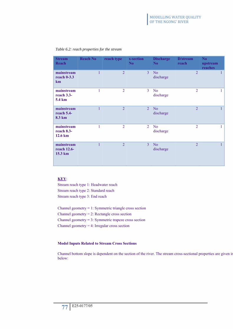
MODELLING WATER QUALITY OF THE NGONG’ RIVER
77 E25-0177/05
Table 6.2: reach properties for the stream
Stream Reach
Reach No reach type x-section No
Discharge No
D/stream reach
No upstream reaches
mainstream reach 0-3.3 km
1 2 3 No discharge
2 1
mainstream reach 3.3-5.4 km
1 2 3 No discharge
2 1
mainstream reach 5.4-8.3 km
1 2 2 No discharge
2 1
mainstream reach 8.3-12.6 km
1 2 2 No discharge
2 1
mainstream reach 12.6-15.3 km
1 2 3 No discharge
2 1
KEY: Stream reach type 1: Headwater reach Stream reach type 2: Standard reach Stream reach type 3: End reach
Channel geometry = 1: Symmetric triangle cross section Channel geometry = 2: Rectangle cross section Channel geometry = 3: Symmetric trapeze cross section Channel geometry = 4: Irregular cross section
Model Inputs Related to Stream Cross Sections
Channel bottom slope is dependent on the section of the river. The stream cross-sectional properties are given inbelow:

MODELLING WATER QUALITY OF THE NGONG’ RIVER
78 E25-0177/05
Table 6.3: stream cross-section properties
valid distance
x-section No manning's n x-section type x-section data
B i
mainstream reach 0-3.3 km
1 0.048 3 0.30 0
mainstream reach 3.3-5.4 km
1 0.070 3 1.30 0.021212121
mainstream reach 5.4-8.3 km
1 0.015 2 0.60 0.028571429
mainstream reach 8.3-12.6 km
1 0.015 2 4.00 0.034482759
mainstream reach 12.6-15.3 km
1 0.070 3 2.50 0.006976744
Model Inputs Related to Diffuse Loads without Flow
(the diffuse loads are not known in this experiment)
Model Inputs Related to Diffuse Loads with Flow
(the diffuse loads are not known in this experiment)
6.1.3 Hydraulic Calculations: In order to calculate the changes in the concentration of a water quality parameter along the
stream, flows and depths along the stream should be known. As measurement of these
parameters along the stream is not possible, they should be calculated. As the dispersion is
neglected, and the model is a steady state model, flows and depths will be calculated by
Manning Formula.
v = R2/3i1/2 Equation 6.1

MODELLING WATER QUALITY OF THE NGONG’ RIVER
79 E25-0177/05
Where:
v = velocity
n= Manning roughness coefficient
R= Hydraulic radius = wet area/wet perimeter (m)
i= Channel bed slope
Hydraulic calculations shall be carried out for 2 principle types of cross-sections; namely
symmetrical trapezoidal and symmetrical rectangular cross-sections. The details of channel
properties are given in the table below:
Table 6.4: channel properties at sampling stations
sample station Name SHAPE CHANNEL
DESCRIPTION
Manning’s n
1 Kariani Dam sym trapeze clean, winding,
some pools and
shoals
0.040
2 Jamhuri Dam
outlet
sym trapeze same as above,
lower stages,
more ineffective
slopes and
sections
0.048
3 Kibera bridge sym trapeze sluggish reaches,
weedy,
0.070
4 Weir of Nairobi
dam
sym rectangle Float finish
concrete
0.015
5 Dunga Rd sym rectangle Float finish
concrete
0.015
6 Outer-ring Rd sym trapeze sluggish reaches,
weedy,
0.070
(Chow, 1959).
6.1.4 Water quality calculations Each of the pollutant types has its own unique equation explaining the distribution of pollutants
along its profile.
6.1.4.1 BOD Under aerobic conditions, BOD is calculated using the following formula:

MODELLING WATER QUALITY OF THE NGONG’ RIVER
80 E25-0177/05
L = L0 exp (-Kr ) Equation 6.2
Where,
x : Distance along the stream reach (km)
U : Current velocity along the stream reaches (m·s-1)
L0 : BOD concentration at the beginning of stream reaches (mg·L-1)
Kr : Total BOD utilization rate (oxidation and settling) (day-1)
L : BOD concentration (mg·L-1)
The process of non-dimensionalization (the partial and full removal of units from an equation
involving physical quantities by a suitable substitution of variables) results in the following
equation:
L = L0 exp
. Equation 6.2b
6.1.4.2 Ammonia nitrogen Under aerobic conditions, ammonia nitrogen is calculated using Equation 6.3
N2 = N2,0 exp(-nitr2,2 ) Equation 6.3
Where,
x : Distance along the stream reach (km)
U : Current velocity along the stream reaches (m·s-1)
nitr2,2 : Total ammonium nitrogen utilization rate (utilization by plants and phytoplankton,
nitrification) (day-1)
N2,0 : Ammonium nitrogen concentration at the beginning of stream reach (mg·L-1)
N2 : Ammonium nitrogen concentration (mg·L-1)
The process of non-dimensionalization (the partial and full removal of units from an equation
involving physical quantities by a suitable substitution of variables) results in the following
equation:
N2 = N2,0 exp,
.) Equation 6.3b

MODELLING WATER QUALITY OF THE NGONG’ RIVER
81 E25-0177/05
6.1.4.3 Nitrate nitrogen Under aerobic conditions, nitrate nitrogen is calculated by Equation 2.4
N3 = ,, ,
[ exp (-nitr2,2 ) –exp(-nitr3,3 ) ] N2,0 + [ exp(-nitr3,3 ) ] N3,0
Equation 6.4
Where,
nitr2,2 : Total ammonium nitrogen utilization rate (utilization by plants and phytoplankton,
nitrification) (day-1)
nitr2,3 : Nitrification rate (day-1)
nitr3,3 : Total nitrate nitrogen utilization rate (utilization by plants and phytoplankton,
denitrification) (day-1)
N2,0 : Ammonium nitrogen concentration at the beginning of stream reach (mg·L-1)
N3,0 : Nitrate nitrogen concentration at the beginning of stream reach (mg·L-1)
N3 : Nitrate nitrogen concentration (mg·L-1)
The process of non-dimensionalization (the partial and full removal of units from an equation
involving physical quantities by a suitable substitution of variables) results in the following
equation:
N3 = ,, ,
* .
[ exp (-nitr2,2 ) – exp(-nitr3,3 ) ] N2,0
+ .
[exp (-nitr3,3 ) ] N3,0 Equation 6.4b
6.1.4.4 Nitrite Nitrogen The general formula for the calculation of nitrogen oxide compound concentrations is given by
Equation 2.5
N4 = ,, ,
[ exp (-nitr2,2 ) –exp(-nitr4,3 ) ] N2,0
+ [ exp (-nitr4,3 ) ] N4,0 Equation 6.5

MODELLING WATER QUALITY OF THE NGONG’ RIVER
82 E25-0177/05
Where:
nitr2,3: Nitrification rate constant (day -1)
nitr2,2 : Total ammonium nitrogen utilization rate (utilization by plants and phytoplankton,
nitrification) (day-1)
nitr4,3: Total nitrite nitrogen utilization rate constant.
N2,0 : Ammonium nitrogen concentration at the beginning of stream reach (mg·L-1)
N4,0 : Nitrite nitrogen concentration at the beginning of stream reach (mg·L-1)
The process of non-dimensionalization (the partial and full removal of units from an equation
involving physical quantities by a suitable substitution of variables) results in the following
equation:
N4 = ,, ,
*.
[ exp (-nitr2,2 ) –exp(-nitr4,3 ) ] N2,0
+ .
[ exp (-nitr4,3 ) ] N4,0 Equation 6.5b
6.1.4.5 Phosphate phosphorus Under aerobic conditions, phosphate phosphorus concentration is calculated by Equation 2.6
P2 = P2,0 exp (- phos2,2 ) Equation 6 .6
where,
x : Distance along the stream reach (km)
U : Current velocity along the stream reaches (m·s-1)
phos2,2 : Total phosphate phosphorus utilization rate (utilization by plants and
phytoplankton etc.) (day-1)
P1,0 : Organic phosphorus concentration at the beginning of stream reach (mg·L-1)
P2,0 : Phosphate phosphorus concentration at the begin of stream reach (mg·L-1)
P2 : Phosphate phosphorus (mg·L-1)

MODELLING WATER QUALITY OF THE NGONG’ RIVER
83 E25-0177/05
The process of non-dimensionalization (the partial and full removal of units from an equation
involving physical quantities by a suitable substitution of variables) results in the following
equation:
P2 = P2,0 exp ,
.) Equation 6.6b
6.2 Solution to model equations and Preliminary test application: Using regression analysis, the following solutions were derived for the equations representing
the BOD and nutrient loading in the river:
6.2.1 BOD The solved model equation gives the equation:
L = L0 exp(0.000116x + 0.013587U -0.1545) Equation 6.7
The co-efficient of determination for this formula (r2) is 0.885453
Thus Kr = - 8.538*10-3 (day -1)
Results for the regression analysis are shown in appendix 9.6.1
6.2.2 Ammonia The solved model equation is:
N2 = N2,0 exp (0.00016x + 0.411692U -0.23777) Equation 6.8
The co-efficient of determination for this formula (r2) is 0.588204
Thus nitr2,2= - 3.886*10-4 (day -1)
Results for the regression analysis are shown in appendix 9.6.2
6.2.3 Nitrate The solved model equation is:
N3 = -52.48 [exp(0.00016x + 0.411692U -0.23777)-(exp(0.004063 )] N2,0
+[0.004063 ] N3,0
= N3,0 exp(0.0000193x + 0.143822U – 0.01228) Equation 6.9
Thus nitr2,2 : - 3.886*10-4 (day -1)
nitr2,3 : 0.19284 (day -1)

MODELLING WATER QUALITY OF THE NGONG’ RIVER
84 E25-0177/05
nitr3,3 : - 0.004063 (day -1)
The co-efficient of determination for this formula (r2) is 0.32563
Results for the regression analysis are shown in appendix 9.6.3
6.2.4 Nitrite The solved model equation is:
N4 = -13.25 [exp(0.00016x + 0.411692U -0.23777)-(exp(-0.00015524 )] N2,0
+(-0.00015524 ) N4,0
= N4,0 exp(0.000085x – 0.13799U + 0.328836) Equation 6.10
The co-efficient of determination for this formula (r2) is 0.279224
Thus nitr2,2 : - 3.886*10-4 (day -1)
nitr2,3 : 0.19284 (day -1)
nitr4,3 : -0.00015524 (day -1)
Results for the regression analysis are shown in appendix 9.6.4
6.2.5 Phosphates The solved model equation is:
P = P0 exp (0.000131x + 0.092408U – 0.25538) Equation 6.11
The co-efficient of determination for this formula (r2) is 0.595935
Thus phosp2,2 = 1.4176 * 10 -3 (day -1)
Results for the regression analysis are shown in appendix 9.6.5
6.3 Model Verification and implementation: The model is tested using the results from the last sampling exercise done on the 17th of
October 2010. The flow properties (U) were assumed to be the same as the average used in the
calibration of the model.
The results from the tests are given in the table below. The values of the concentrations at the
beginning of the reach are tested and used to determine the concentrations at the other sections
of the profile.
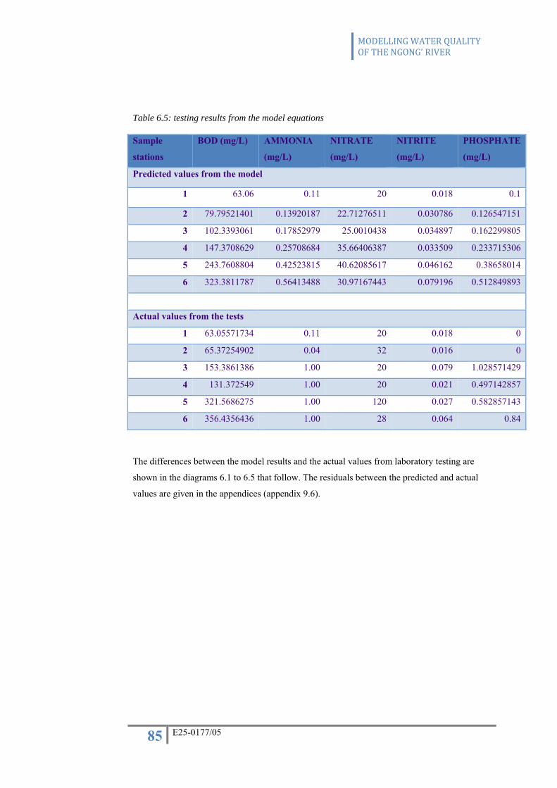
MODELLING WATER QUALITY OF THE NGONG’ RIVER
85 E25-0177/05
Table 6.5: testing results from the model equations
Sample
stations
BOD (mg/L) AMMONIA
(mg/L)
NITRATE
(mg/L)
NITRITE
(mg/L)
PHOSPHATE
(mg/L)
Predicted values from the model
1 63.06 0.11 20 0.018 0.1
2 79.79521401 0.13920187 22.71276511 0.030786 0.126547151
3 102.3393061 0.17852979 25.0010438 0.034897 0.162299805
4 147.3708629 0.25708684 35.66406387 0.033509 0.233715306
5 243.7608804 0.42523815 40.62085617 0.046162 0.38658014
6 323.3811787 0.56413488 30.97167443 0.079196 0.512849893
Actual values from the tests
1 63.05571734 0.11 20 0.018 0
2 65.37254902 0.04 32 0.016 0
3 153.3861386 1.00 20 0.079 1.028571429
4 131.372549 1.00 20 0.021 0.497142857
5 321.5686275 1.00 120 0.027 0.582857143
6 356.4356436 1.00 28 0.064 0.84
The differences between the model results and the actual values from laboratory testing are
shown in the diagrams 6.1 to 6.5 that follow. The residuals between the predicted and actual
values are given in the appendices (appendix 9.6).
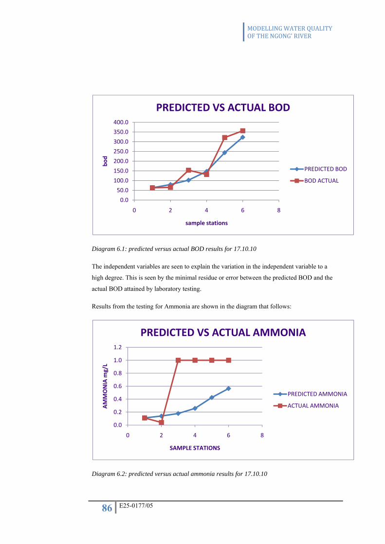
MODELLING WATER QUALITY OF THE NGONG’ RIVER
86 E25-0177/05
Diagram 6.1: predicted versus actual BOD results for 17.10.10
The independent variables are seen to explain the variation in the independent variable to a
high degree. This is seen by the minimal residue or error between the predicted BOD and the
actual BOD attained by laboratory testing.
Results from the testing for Ammonia are shown in the diagram that follows:
Diagram 6.2: predicted versus actual ammonia results for 17.10.10
0.0
50.0
100.0
150.0
200.0
250.0
300.0
350.0
400.0
0 2 4 6 8
bod
sample stations
PREDICTED VS ACTUAL BOD
PREDICTED BOD
BOD ACTUAL
0.0
0.2
0.4
0.6
0.8
1.0
1.2
0 2 4 6 8
AMMONIA m
g/L
SAMPLE STATIONS
PREDICTED VS ACTUAL AMMONIA
PREDICTED AMMONIA
ACTUAL AMMONIA

MODELLING WATER QUALITY OF THE NGONG’ RIVER
87 E25-0177/05
In the case of ammonia, the results from the model equations show a wide difference with the
actual ammonia results obtained from the laboratory testing. The validation of the model can
be determined further by the collection of more samples under different environmental
conditions for use in model calibration.
The results for the testing of nitrates are shown in the diagram that follows:
Diagram 6.3: predicted versus actual nitrate results for 17.10.10
For all stations except station 5, the results from the model equations are seen to be
approximately equal to the values gotten through laboratory testing. The nitrate value for
sample station 5 is taken, in analysis, as an ‘outlier’-a value that can be a source of error and
affects the degree to which the model explains the variance in the dependent variable.
The results from the expected and actual Nitrite concentrations are shown in the diagram
below:
0.0
20.0
40.0
60.0
80.0
100.0
120.0
140.0
0 2 4 6 8
NITRA
TE m
g/L
SAPLE STATIONS
PREDICTED VS ACTUAL NITRATE
PREDICTED NITRATE
ACTUAL NITRATE

MODELLING WATER QUALITY OF THE NGONG’ RIVER
88 E25-0177/05
Diagram 6.4: predicted versus actual nitrite results for 17.10.10
The predicted concentrations are consistently higher than the actual concentrations for all
stations except station 3, which shows a nitrite concentration of 1.00 mg/L that could be the
result of high levels of pollution into the river.
The results from the testing of the equation for the prediction of phosphate concentration when
compared to actual results from laboratory testing yielded the following diagram:
Diagram 6.5: predicted versus actual phosphates results for 17.10.10
0.00.00.00.00.00.10.10.10.10.1
0 2 4 6 8
NITRITE
mg/L
SAMPLE STATIONS
PREDICTED VS ACTUAL NITRITE
PREDICTED NITRITE
ACTUAL NITRITE
0.0
0.2
0.4
0.6
0.8
1.0
1.2
0 2 4 6 8
PHOSPHATE
mg/L
SAMPLE STATIONS
PREDICTED VS ACTUAL PHOSPHATES
PREDICTED PHOSPHATES
ACTUAL PHOSPHATES

MODELLING WATER QUALITY OF THE NGONG’ RIVER
89 E25-0177/05
Phosphate concentration from the prediction in the model equation increased exponentially
along the profile of the river. They were however lower than the actual results.
6.4 Accounting for pollution input into the river: A key component of any model is its ability to predict the input of pollutants into the river at
various sections along the profile.
In this model the quantity of pollutant that will be taken as discharged into the river at any
section is the difference between the predicted value at the particular chainage and at the flow
velocity specified minus the predicted value at the last pre-determined sample station.
6.5 Capabilities and Limitations of the Water Quality Model The model is a steady state water quality model that can estimate biochemical oxygen demand,
ammonium nitrogen, nitrate nitrogen and phosphate phosphorus concentrations along streams
for steady state. Because it is relatively easy to use and understand, it can be considered as a
useful tool that fills in the gap between manual calculations and complex models.
Its limitations are listed below:
• Hydraulic calculations can only be conducted for uniform flow. Therefore, the depths
and velocities calculated at the river sections, where flow velocities are low or rapidly
changing flow conditions occur will contain errors.
• The model simulates the transport only using advection and neglects dispersion.
Therefore, errors will increase for the aquatic environments (such as transitional
waters reaching the sea), where dispersion is important.
• No correction is made in parameters for deviations in temperature of samples from the
standard 20⁰C.
• Nitrogen and phosphorus cycles do not affect each other like in real aquatic
ecosystems through primary production. Therefore, errors will increase for the aquatic
environments, where primary production is important.
• Linear regression as used to determine the parameters and utilisation constants does
not adequately explain the variance in the data for all nutrient pollutants. The co-
efficient of determination (r2) in some cases is less than 40%.
• We need to collect a lot more data to verify the predictions of the model equations.
This is a key constraint.
MODELLING WATER QUALITY OF THE NGONG’ RIVER
90 E25-0177/05
6.6 Discussion: Water quality analyses based on the monitored data do not provide pollutant load distribution
along the entire river network. Such type of spatial information can only be generated if stream
water quality models are used to interpolate the available data. Therefore, the water quality
model developed in this study will further be controlled with the water quality assessment
realized for the selected data.
Water quality models have the advantage of including the essential mechanisms that take place
in the stream directly to the interpolation process, unlike other interpolation and statistical
methods that use/relate data from different locations numerically and partly consider the nature
of the stream. Models also provide other advantages and benefits for further stages of water
pollution control. By using models it is possible to generate scenarios, establish management
plans, project the probable environmental impacts, and estimate the costs of the measures to be
taken. Thus, water quality models are being used as decision-support system tools since they
can comment “better” on the possible future conditions of the aquatic ecosystems and have a
scientific basis for better management plans.
6.7 Conclusions: This study mainly consists of two parts. In the first one, water quality assessment is realized for
the Ngong' River by carrying out laboratory testing on the samples obtained from the pre-
selected sampling stations. The number of monitoring stations needs to be increased in order to
make a better water quality assessment.
Due to the data constraints highlighted in the limitations of the study, the modelling study has
not reached its final stage. The model itself is more suitable for screening through many
different water quality management options, and for determining the ones that could be further
investigated rather than predicting the benefits of individual management options. As more
data become available, more advanced watershed/water quality models with further
components could be developed.
The results derived from the model were found, in some instances, to be consistent with water
quality assessment for some of the pollutant types and not so in others. Such an inconsistency
between the findings of the measured and modelled values indicates that the developed model
needs further refinement by considering other variables that could directly affect and thus
predict the concentrations of these pollutant concentrations. This is essential before the model
can be used for predicting future water quality in case of any changes in the organic matter
and/or nutrient loads.

MODELLING WATER QUALITY OF THE NGONG’ RIVER
91 E25-0177/05
7. RECOMMENDATIONS AND WAY FORWARD The pollutant levels within Ngong' River needs to be considered and adequate measures need
to be taken to improve monitoring and deal with inflow of pollutants into the river. The
examples given are not full but instead, present a sample of practical and tangible actions that
can be implemented, in an effort to reduce pollution.
a. Continuous monitoring of the river pollution using the selected base stations.
b. Further study to understand the behaviour of the pollutants and their relationship with
a variety of variables.
c. Industrial discharges should be stopped through efforts by the industries to take
measures to address pollution produced as waste from their production processes
d. Address the discharge of human waste into the river especially at the sections where is
passes through the slum areas- Kibera, Mukuru. This can be initiated by relocation of
human settlement or by diversion of river water, either around such sections or within
enclosed conduits underground.
e. Clean up action plan should be drawn to involve the communities that rely on the
water from Ngong' river.
f. Some technical and financial support should be considered in developing technologies
to treat discharges from the industries within their individual premises.
g. Community sensitisation and awareness programmes to encourage a healthy attitude
towards water resource conservation and use.
h. Polluter- pays principle should be considered and it’s viability as a means of reducing
pollution should be investigated. It can be initiated in order to determine its effect on
lowering the pollution levels of the river.
i. Engineering solutions such as channelling the river or introduction of flow weirs,
especially in areas where stagnant pools exist.
The way forward is:
a. Develop techniques to consistently monitor the levels of pollution within the river and
other freshwater sources.
b. Capacity development is crucial in local authorities to enable them to discharge their
duties to monitor and prevent pollution of riverine water sources.
c. Develop an action plan to coordinate the cleaning effort of Ngong' river and it’s
‘sister’rivers.
MODELLING WATER QUALITY OF THE NGONG’ RIVER
92 E25-0177/05
8. REFERENCES: Ali Erturk, Alpaslan Ekdal, Melike Gurel, Kiziltan Yuceil, Aysegul Tanik, 2004. “Use of
mathematical models to estimate the effect of nutrient loadings on small streams.”
Ali Erturk, Melike Gurel, Mansoor Ahmed Baloch, Teoman Dikerler, Evren Varol,
Neslihan Akbulut, and Aysegul Tanik, 2006. “Application of Watershed Modeling
System (WMS) for Integrated Management of a Watershed in Turkey.”
Ali Erturk, 2009. “Simple Stream Model - Version 0.9.5 User Guide and Reference
Manual”
Bartram J. and Balance R., 1995. “Water Quality Monitoring – a practical guide to the
design and implementation of freshwater quality studies and monitoring programmes.”
Bende-Michl, U.2009. “Complementary water quality modelling to support natural
resource management decision making in Australia”
Chapman D. and Kimstach V., 1997. “Water Quality Assessments- A Guide To The Use
Of Biota, Sediments And Water In Environmental Monitoring”,
Gevearts, E. A. L. 1971. Hydrology of the Nairobi Are, Technical report. Water
Department. Howard G. 2002. Private communication (IUCN)
Gonzales, A. E, 2001. Statistical Techniques Applied to Optimization of Sampling
Campaigns in a Reservoir. Proceedings of the third International Workshop on Regional
Approaches to Reservoir Development and Management in the La Plata River Basin:
Informed decision Processes for Sustainable Development of Reservoirs. UNEP-IETC
pp. 262.
Hem J. D., “Study and interpretation of the Chemical Characteristics of Natural Waters”,
1989. WHO Guidelines for Drinking Water Quality. Volume 2. Health Criteria and other
supporting information.
Himesh S., Rao C.V.C. and Mahajan A.U, 2000. “Calibration and Validation of Water
Quality Model, Case 1. River.”
Issaias, I. 2000. Environmental Impact of Urbanization on Water Resources-A case study

MODELLING WATER QUALITY OF THE NGONG’ RIVER
93 E25-0177/05
on Nairobi Dam. Imperial College of Science, Technology and Medicine
(University of London).100pp.
Kithia, S. M 2001. The effects of Land Use Changes on the Hydrology and Water Quality
of Upper-Athi River Basin, Kenya. Programme and Abstracts for VLIR-IUCUoN Annual
Postgraduate Seminars 2001.
Krhoda, G. 2002. Nairobi River Basin Project Phase II: The Monitoring and Sampling
Strategy for Ngong/Motoine River. (In press, pp. 55).
Mooney D., Swift R., 1999. “A course in mathematical Modelling.”
Ndede, H. 2002. Baseline Survey and Environmental Impact Assessment for the Nairobi
River Basin Project-Phase II. (In press, pp. 50).
Ngecu & Gaciri 1998. Urbanisation Impact on the Water Resources with major third
world cities: A case study of Nairobi and its Environs. Episodes, Vol. 21 no. 4. PP226.
Ohayo-Mitoko, G. 1996. Concentrations of Heavy Metals, Organochlorine Pesticides,
Organic and Microbial Pollution in the Nairobi River and it’s Tributaries. Dissemination
Workshop on “Concentrations of Heavy Metals, Organochlorine pesticides, Organic and
Microbial Pollution in the Nairobi River and it’s Tributaries”. Sustainable Development
Consultants. 113pp.
Olago & Aketch 2000. Pollution Assessment in Nairobi River Basin. Pollution
Assessment Report of The Nairobi River Basin. Africa Water Network. Okoth, PF &
Otieno P. (eds).106pp. UNEP, 1999. The Nairobi River Basin Project-Project Summary.
UNEP, pp16.
Peter Reichert, Dietrich Borchardt, Mogens Henze, Wolfgang Rauch, Peter Shanahan,
László Somlyódy, Peter A. Vanrolleghem, 2001. “River Water Quality Model No. 1,
Edited by IWA Task Group on River Water Quality Modelling”
Sharon N. Kahara, 2002. “Characterizing Anthropogenic Sources of Pollution for
Tropical Urban River Management: A Proposed Case Study of the Nairobi River Basin. “
Wandiga, S. O 1996. River Pollution In Developing Countries-A case study III: Effect of
Industrial Discharges on Quality of Ngong River Waters in Kenya. Dissemination

MODELLING WATER QUALITY OF THE NGONG’ RIVER
94 E25-0177/05
Workshop on “Concentrations of Heavy Metals, Organochlorine pesticides, Organic and
Microbial Pollution in the Nairobi River and its Tributaries”. Sustainable Development
Consultants. 113pp.

MODELLING WATER QUALITY OF THE NGONG’ RIVER
95 E25-0177/05
9. APPENDICES:
9.1 Budget: The budget for undertaking the project is summarised in the table below:
ACTIVITY SHILLINGS
BACKGROUND DATA FROM NRBP/NEMA/WARMA
400
SAMPLE COLLECTION/ LABOUR/ MATERIALS
1,500
PRINTING WORK 600
TRANSPORT 2,500
CHEMICAL ANALYSIS (LABORATORY WORK)
5,000
TOTAL 10,000

MODELLING WATER QUALITY OF THE NGONG’ RIVER
96 E25-0177/05
9.2 Working schedule:
The working schedule for the project is shown here:

MODELLING WATER QUALITY OF THE NGONG’ RIVER
97 E25-0177/05
9.3 The tabulated results from NRDP- Phase II, UON/UNEP project, Feb- Nov 2003, Final report:
The results from the initial study carried out in the NRDP- Phase II are shown in Table 9.1 and Table 9.2 below:
They were much higher in the dry weather than in the wet weather (NRDP- Phase II, UON/UNEP project, Feb- Nov 2003, Final report).
TABLE 9.1
TABLE 9.2

MODELLING WATER QUALITY OF THE NGONG’ RIVER
98 E25-0177/05
9.4 The plotted results from NRDP- Phase II, UON/UNEP project, Feb- Nov 2003, Final report:
Diagram 9.1 shows the ammonia concentration along the river profile, diagram 9.2 shows the
nitrite concentration and diagram 9.3 shows the phosphate concentration along the profile.
Diagram 9.1: ammonia concentration along the river (source: fig 3.4 (c) NRDP- Phase II,
UON/UNEP project, Feb- Nov 2003, Final report.)
Diagram 9.2: nitrite concentration along the river (source: fig 3.4 (b) NRDP- Phase II,
UON/UNEP project, Feb- Nov 2003, Final report.)

MODELLING WATER QUALITY OF THE NGONG’ RIVER
99 E25-0177/05
Diagram 9.3: phosphate concentration along the Ngong River (source fig 3.4 (a) NRDP-
Phase II, UON/UNEP project, Feb- Nov 2003, Final report.)
9.5 Manning’s co-efficient (Chow, 1959): Mannning’s co-efficient for main channel for use in the manning’s formula was taken from the table below:
Table 9.3: table showing Manning’s n (Chow, 1959).
Type of Channel and Description Minimum Normal Maximum
Natural streams - minor streams (top width at floodstage < 100 ft)
1. Main Channels
a. clean, straight, full stage, no rifts or deep pools 0.025 0.030 0.033
b. same as above, but more stones and weeds 0.030 0.035 0.040
c. clean, winding, some pools and shoals 0.033 0.040 0.045
d. same as above, but some weeds and stones 0.035 0.045 0.050
e. same as above, lower stages, more ineffective slopes and sections
0.040 0.048 0.055
f. same as "d" with more stones 0.045 0.050 0.060
g. sluggish reaches, weedy, deep pools 0.050 0.070 0.080
h. very weedy reaches, deep pools, or floodways with heavy stand of timber and underbrush
0.075 0.100 0.150

MODELLING WATER QUALITY OF THE NGONG’ RIVER
100 E25-0177/05
9.6 Summary output from regression analysis for modelling: Regression analysis was used to find the solutions to the model equations. The natural log of the dependent variable was calculated to determine the exponential trendline that best explains the data. The summary output from the determination of the regression line that best fits to explain the pollution distribution along the profile of the river is given below:
9.6.1 BOD For the model, the independent variables were taken to be ‘x’ and ‘U’. The dependent variable was ‘ln’ which is the natural log of (L/L0). The table is shown below.
Table 9.4: table for determination of trendline fitting the data.
sample station
x U x/U L L/Lo ln
1 0 0 0 67.72471365 1 0
2 3300 0.525854867 6275.49578 58.36206562 0.861754336 -0.14878504
3 5400 0.910803375 5928.831788 147.1567657 2.172866562 0.776047292
4 8300 2.990619611 2775.344604 136.3020773 2.012589938 0.699422419
5 12600 3.31706844 3798.53483 295.5348476 4.363766662 1.473335598
6 15300 1.068154092 14323.77606 329.5402834 4.865879318 1.582247443
Summary output:
Regression Statistics Multiple R 0.940985 R Square 0.885453 Adjusted R Square 0.809089 Standard Error 0.314295 Observations 6
ANOVA df SS MS F
Regression 2 2.290748 1.145374 11.59507 Residual 3 0.296343 0.098781 Total 5 2.587091
Coefficients Standard
Error t Stat P-value Intercept -0.1545 0.22919 -0.67411 0.548537 x 0.000116 3.06E-05 3.772518 0.03261 U 0.013587 0.129702 0.104752 0.923183

MODELLING WATER QUALITY OF THE NGONG’ RIVER
101 E25-0177/05
RESIDUAL OUTPUT
Observation Predicted
ln Residuals 1 -0.1545 0.154499 2 0.234059 -0.38284 3 0.482006 0.294041 4 0.845445 -0.14602 5 1.346873 0.126463 6 1.628383 -0.04614
9.6.2 Ammonia For the model, the independent variables were taken to be ‘x’ and ‘U’. The dependent variable was ‘ln’ which is the natural log of (N2/N2,0). The table is shown below.
Table 9.5: table for determination of trendline fitting the data.
sample station
x U x/U AMMONIA N2/N2,0 ln
1 0 0 0 0.07 1 0
2 3300 0.525854867 6275.49578 0.02 0.285714286 -1.25276297
3 5400 0.910803375 5928.831788 1.00 14.28571429 2.659260037
4 8300 2.990619611 2775.344604 1.00 14.28571429 2.659260037
5 12600 3.31706844 3798.53483 1.00 14.28571429 2.659260037
6 15300 1.068154092 14323.77606 1.00 14.28571429 2.659260037
Summary output:
Regression Statistics Multiple R 0.766944 R Square 0.588204 Adjusted R Square 0.313673 Standard Error 1.443434 Observations 6
ANOVA df SS MS F
Regression 2 8.928127 4.464063 2.142579 Residual 3 6.250501 2.0835 Total 5 15.17863
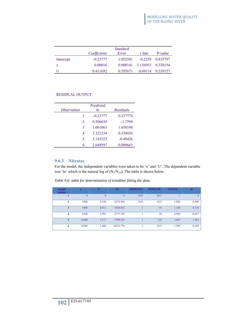
MODELLING WATER QUALITY OF THE NGONG’ RIVER
102 E25-0177/05
Coefficients Standard
Error t Stat P-value Intercept -0.23777 1.052581 -0.2259 0.835797 x 0.00016 0.000141 1.136953 0.338154 U 0.411692 0.595671 0.69114 0.539157
RESIDUAL OUTPUT
Observation Predicted
ln Residuals 1 -0.23777 0.237774 2 0.506634 -1.7594 3 1.001063 1.658198 4 2.321234 0.338026 5 3.143523 -0.48426 6 2.649597 0.009663
9.6.3 Nitrates For the model, the independent variables were taken to be ‘x’ and ‘U’. The dependent variable was ‘ln’ which is the natural log of (N3/N3,0). The table is shown below.
Table 9.6: table for determination of trendline fitting the data.
sample station
x U x/U AMMONIA NITRATE N3/N3,0 ln
1 0 0 0 0.07 30.5 1 0
2 3300 0.526 6275.496 0.02 45.5 1.492 0.400
3 5400 0.911 5928.832 1 35 1.148 0.138
4 8300 2.991 2775.345 1 30 0.984 -0.017
5 12600 3.317 3798.535 1 110 3.607 1.283
6 15300 1.068 14323.776 1 39.5 1.295 0.259

MODELLING WATER QUALITY OF THE NGONG’ RIVER
103 E25-0177/05
Summary output:
Regression Statistics Multiple R 0.57064 R Square 0.32563 Adjusted R Square -0.12395 Standard Error 0.515593 Observations 6
ANOVA df SS MS F
Regression 2 0.38509 0.192545 0.7243 Residual 3 0.797509 0.265836 Total 5 1.1826
Coefficients Standard
Error t Stat P-value Intercept -0.01228 0.375981 -0.03265 0.976004 x 1.93E-05 5.03E-05 0.384919 0.725965 U 0.143822 0.212773 0.675939 0.547522
RESIDUAL OUTPUT
Observation Predicted ln Residuals 1 -0.01228 0.012276 2 0.127195 0.272791 3 0.223185 -0.08556 4 0.578411 -0.59494 5 0.708549 0.574204 6 0.437341 -0.17877
9.6.4 Nitrites For the model, the independent variables were taken to be ‘x’ and ‘U’. The dependent variable was ‘ln’ which is the natural log of (N4/N4,0). The table is shown below.

MODELLING WATER QUALITY OF THE NGONG’ RIVER
104 E25-0177/05
Table 9.7: table for determination of trendline fitting the data.
sample station
x U x/U AMMONIA NITRITE N4/N4,0 ln
1 0 0 0 0.07 0.06 1 0
2 3300 0.526 6275.496 0.02 0.06 1 0
3 5400 0.911 5928.832 1 0.44 7 1.946
4 8300 2.991 2775.345 1 0.10 1.6 0.470
5 12600 3.317 3798.535 1 0.15 2.4 0.875
6 15300 1.068 14323.776 1 0.23 3.6 1.281
Summary output:
Regression Statistics Multiple R 0.528417 R Square 0.279224 Adjusted R Square -0.20129 Standard Error 0.839073 Observations 6
ANOVA df SS MS F
Regression 2 0.818228 0.409114 0.581091 Residual 3 2.112133 0.704044 Total 5 2.930361
Coefficients Standard
Error t Stat P-value Intercept 0.328836 0.61187 0.537428 0.628278 x 8.5E-05 8.18E-05 1.038907 0.375225 U -0.13799 0.346266 -0.39852 0.716917
RESIDUAL OUTPUT
Observation Predicted
ln Residuals 1 0.328836 -0.32884 2 0.536688 -0.53669 3 0.662015 1.283895 4 0.621441 -0.15144 5 0.941785 -0.06632
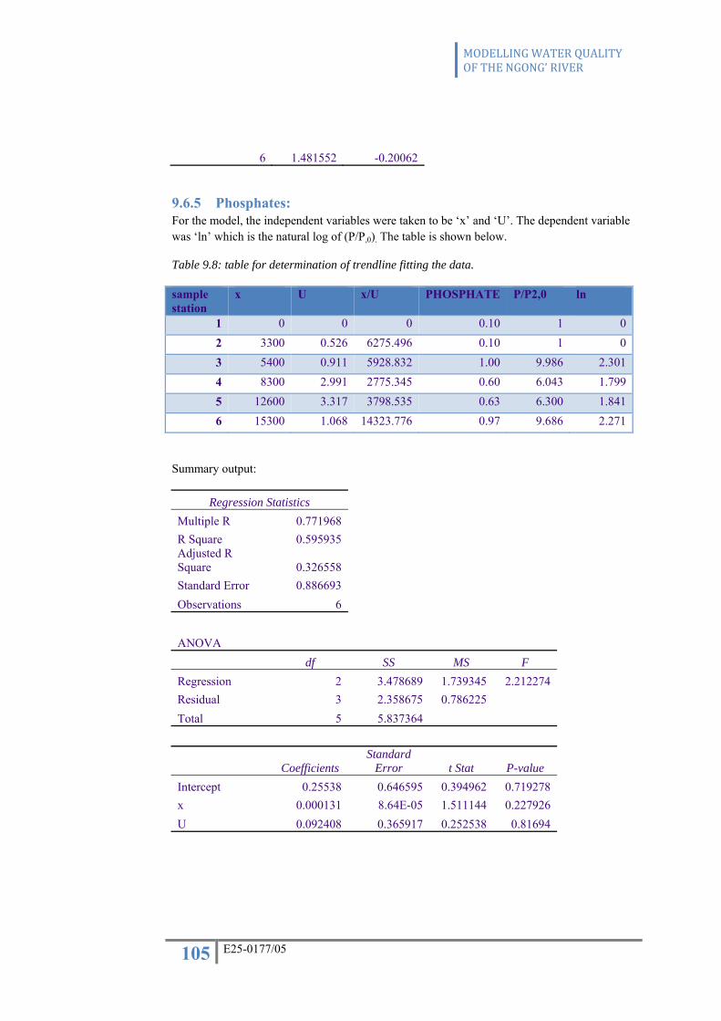
MODELLING WATER QUALITY OF THE NGONG’ RIVER
105 E25-0177/05
6 1.481552 -0.20062
9.6.5 Phosphates: For the model, the independent variables were taken to be ‘x’ and ‘U’. The dependent variable was ‘ln’ which is the natural log of (P/P,0). The table is shown below.
Table 9.8: table for determination of trendline fitting the data.
sample station
x U x/U PHOSPHATE P/P2,0 ln
1 0 0 0 0.10 1 02 3300 0.526 6275.496 0.10 1 03 5400 0.911 5928.832 1.00 9.986 2.3014 8300 2.991 2775.345 0.60 6.043 1.7995 12600 3.317 3798.535 0.63 6.300 1.8416 15300 1.068 14323.776 0.97 9.686 2.271
Summary output:
Regression Statistics Multiple R 0.771968 R Square 0.595935 Adjusted R Square 0.326558 Standard Error 0.886693 Observations 6
ANOVA df SS MS F
Regression 2 3.478689 1.739345 2.212274 Residual 3 2.358675 0.786225 Total 5 5.837364
Coefficients Standard
Error t Stat P-value Intercept 0.25538 0.646595 0.394962 0.719278 x 0.000131 8.64E-05 1.511144 0.227926 U 0.092408 0.365917 0.252538 0.81694

MODELLING WATER QUALITY OF THE NGONG’ RIVER
106 E25-0177/05
RESIDUAL OUTPUT
Observation Predicted ln Residuals 1 0.25538 -0.25538 2 0.735002 -0.735 3 1.044866 1.25629 4 1.615841 0.183036 5 2.207651 -0.3671 6 2.352494 -0.08184
9.7 SISMOD OPERATION The operation of SISMOD, which was modified for the purposes of this study, has the following input requirements:
Model Input Requirements:
Essential Information
Essential information should only be entered once in following order:
Record 1
Description line
Record 2
Description line
Record 3
To the same line in the following order
• Number of stream reaches (positive integer)
• Number of headwaters (positive integer)
• Number of cross sections (positive integer)
• Number of point loads (positive integer)
• Status of nitrogen cycle modelling (integer, zero or one)
• Status of phosphorus cycle modelling (integer, zero or one)
If the status of the nitrogen cycle is entered as one; water quality variables organic nitrogen,
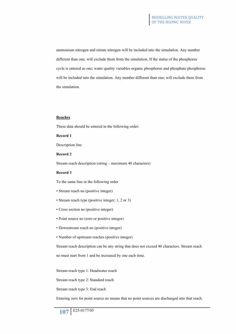
MODELLING WATER QUALITY OF THE NGONG’ RIVER
107 E25-0177/05
ammonium nitrogen and nitrate nitrogen will be included into the simulation. Any number
different than one; will exclude them from the simulation. If the status of the phosphorus
cycle is entered as one; water quality variables organic phosphorus and phosphate phosphorus
will be included into the simulation. Any number different than one; will exclude them from
the simulation.
Reaches
These data should be entered in the following order:
Record 1
Description line
Record 2
Stream reach description (string – maximum 40 characters)
Record 3
To the same line in the following order
• Stream reach no (positive integer)
• Stream reach type (positive integer; 1, 2 or 3)
• Cross section no (positive integer)
• Point source no (zero or positive integer)
• Downstream reach no (positive integer)
• Number of upstream reaches (positive integer)
Stream reach description can be any string that does not exceed 40 characters. Stream reach
no must start from 1 and be increased by one each time.
Stream reach type 1: Headwater reach
Stream reach type 2: Standard reach
Stream reach type 3: End reach
Entering zero for point source no means that no point sources are discharged into that reach.

MODELLING WATER QUALITY OF THE NGONG’ RIVER
108 E25-0177/05
Record 4
Description line entered for the upstream reaches
Record 5
Upstream reach no (integer)
Record 1 should be entered only once. Record 2, Record 3 and Record 4 are entered once for
each stream reach. Record 5 is entered for each stream reach number of upstream reached
(Record 4) times.
If a stream reach is a headwater reach, number of upstream reaches should be entered as one
and the upstream reach should be negative of the headwater no that connects to the stream
reach.
Cross Sections
These data should be entered in the following order:
Record 1
Description line
Record 2
Cross section description (string – maximum 40 characters)
Record 3
To the same line in the following order
• Cross section no (positive integer)
• Slope of the channel bottom (positive real number)
• Manning roughness coefficient (positive real number)
• Channel geometry (1, 2, 3 or 4)
Cross section description can be any string that does not exceed 40 characters. Cross section
no must start from one and be increased by one each time.
Channel geometry = 1: Symmetric triangle cross section
Channel geometry = 2: Rectangle cross section

MODELLING WATER QUALITY OF THE NGONG’ RIVER
109 E25-0177/05
Channel geometry = 3: Symmetric trapeze cross section
Channel geometry = 4: Irregular cross section
Record 4
Description line entered for the cross section geometry
Record 5
To the same line in the following order
• Channel width B if necessary (in metres, positive real number)
• Chamfer slope Z if necessary (positive real number)
Rules to consider when entering Record 5:
• Only chamfer slope Z should be entered for symmetric triangular cross sections.
• Only bed width B should be entered for rectangular cross sections.
• For the symmetric trapezoidal cross sections first the bed width B and then the
chamfer slope Z should be entered
Record 6
Number points as x, y pairs that form the irregular cross section
Record 7
Description line
Record 8
x coordinate and y coordinate