modelling geotechnical heterogeneities using
TRANSCRIPT

minerals
Article
Modelling Geotechnical Heterogeneities UsingGeostatistical Simulation and FiniteDifferences Analysis
Marisa Pinheiro 1,*, Xavier Emery 2,3, Tiago Miranda 1 ID , Luís Lamas 4 and Margarida Espada 4 ID
1 Department of Civil Engineering, ISISE, University of Minho, 4800-058 Guimarães, Portugal;[email protected]
2 Department of Mining Engineering, University of Chile, Santiago 8370448, Chile; [email protected] Advanced Mining Technology Centre, University of Chile, Santiago 8370448, Chile4 Concrete Dams Department, National Laboratory of Civil Engineering, 1700-066 Lisboa, Portugal;
[email protected] (L.L.); [email protected] (M.E.)* Correspondence: [email protected]; Tel.: +351-912-789-989
Received: 30 November 2017; Accepted: 30 January 2018; Published: 7 February 2018
Abstract: Modelling a rock mass in an accurate and realistic way allows researchers to reduce theuncertainty associated with its characterisation and reproduce the intrinsic spatial variability andheterogeneities present in the rock mass. However, there is often a lack of a structured methodology tocharacterise heterogeneous rock masses using geotechnical information available from the prospectionphase. This paper presents a characterization methodology based on the geostatistical simulationof geotechnical variables and the application of a scenario reduction technique aimed at selecting areduced number of realisations able to statistically represent a large set of realisations obtained by thegeostatistical approach. This type of information is useful for a further rock mass behaviour analysis.The methodology is applied to a gold deposit with the goal of understanding its main differences totraditional approaches based on a deterministic modelling of the rock mass. The obtained resultsshow the suitability of the methodology to characterise heterogeneous rock masses, since there wereconsiderable differences between the results of the proposed methodology, mainly concerning thetheoretical tunnel displacements, and the ones obtained with a traditional approach.
Keywords: 3D geological models; geotechnical modelling; geological heterogeneity; uncertaintyassessment; mechanical behaviour analysis
1. Introduction
Existing tools and methodologies used to characterise rock masses have shown limitations inidentifying the natural heterogeneities and in reducing uncertainties related to high spatial variability.Also, their impact on the geomechanical parameters and, consequently, on the overall behaviourof underground works is difficult to predict. In the past years, the use of probabilistic techniques,such as Taylor series and Monte Carlo simulation [1,2], have been able to mitigate these limitations;however, the impact of high levels of heterogeneity in the behaviour of rock masses is still a complextask and not duly solved. More recently, several authors have proposed the use of geostatisticaltechniques that, in contrast to traditional probabilistic techniques, take account of the spatialdependence of the data and allow for the accurate prediction of the unknown values of geomechanicalparameters, such as Rock Quality Designation (RQD), Rock Mass Rating (RMR), and discontinuitiesparameters [3–17]. Furthermore, with geostatistical simulation techniques, several scenarios orrealisations used to represent the variable(s) of interest are obtained, all of which reproduce thespatial correlation structure of the sample data [18].
Minerals 2018, 8, 52; doi:10.3390/min8020052 www.mdpi.com/journal/minerals

Minerals 2018, 8, 52 2 of 19
This paper presents a methodology developed to model the geomechanical parameters ofheterogeneous rock masses. The methodology starts with a probabilistic technique and a geostatisticalsimulation coupled with a clustering technique in order to obtain a reduced number of representativerealisations, following works applied in the mining and petroleum industries [19–23]. With theapplication of the aforementioned methodology, it is possible to map, simultaneously, the uncertaintyassociated with the geomechanical parameters’ quantification, their spatial variability, and theheterogeneities existing in the rock masses at different spatial scales.
To validate the methodology, a numerical analysis of the rock mass mechanical behaviour duringthe excavation of a tunnel will be examined. For this purpose, data from a gold deposit located inthe Atacama Region, northern Chile, will be used. The data include the Rock Mass Rating (RMR)empirical system and the Uniaxial Compressive Strength (UCS) of the intact rock, all extractedfrom mechanical boreholes and laboratory tests. Using this information, a theoretical tunnel willbe modelled, using the proposed methodology to simulate the rock mass properties, and the resultswill be compared with a similar analysis performed using a deterministic approach that assumes therock is a homogeneous mass.
The proposed methodology intends to take a step ahead by implementing geostatistical techniques,which are often assumed to be complex and impractical, mainly in relation to the geomechanicalcharacterisation of rock masses.
2. Proposed Methodology
2.1. General
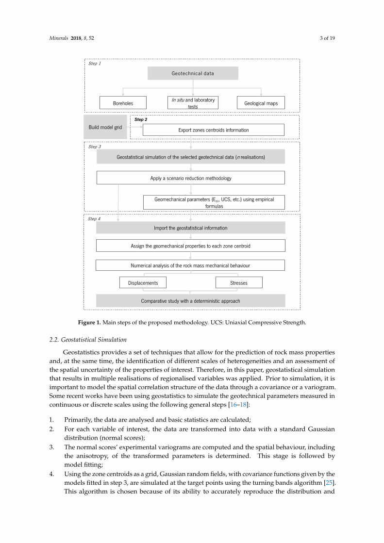
To apply this methodology it is necessary, in a first step, to collate all the available geotechnicalinformation originating from different sources, such as boreholes and in situ and laboratory tests(Figure 1: step 1). Then, a statistical analysis of the available data should be performed in order tooutline the behaviour of the variable(s) of interest through the calculation of the statistical parametersrequired for simulation.
A further preparatory step concerns the development of the grid model selected to represent therock mass block and the underground structures. Once all of the shapes and elements of the modelunder study are defined, the corresponding two-dimensional (2D) or three-dimensional (3D) spatialinformation from all zone centroids is exported so that it can be used in the following rock masscharacterisation methodology (Figure 1: step 2).
Subsequently, the chosen variables are simulated at the target grid points (zone centroids of thegrid). Each variable represents either a geomechanical parameter or an empirical system value used tocharacterise the rock mass. If the variable is an empirical system value, the use of empirical formulasto obtain the values of the geomechanical parameters is an additional required step (Figure 1: step 3).
Based on the simulation results, an important and required step is the application of a dimensionreduction methodology, whose goal is to avoid the computational burden of the following step,the finite differences analysis of the geostatistical realisations. The goal is to guarantee that the subsetof selected realisations is statistically representative of the full set. As a final step, a numerical analysisof the underground structure behaviour using finite difference elements software [24] is performedbased on the selected realisations. (Figure 1: step 4).
Minerals 2018, 8, 52 3 of 19
Minerals 2018, 8, x FOR PEER REVIEW 3 of 19
Figure 1. Main steps of the proposed methodology. UCS: Uniaxial Compressive Strength.
2.2. Geostatistical Simulation
Geostatistics provides a set of techniques that allow for the prediction of rock mass properties and, at the same time, the identification of different scales of heterogeneities and an assessment of the spatial uncertainty of the properties of interest. Therefore, in this paper, geostatistical simulation that results in multiple realisations of regionalised variables was applied. Prior to simulation, it is important to model the spatial correlation structure of the data through a covariance or a variogram. Some recent works have been using geostatistics to simulate the geotechnical parameters measured in continuous or discrete scales using the following general steps [16–18]:
1. Primarily, the data are analysed and basic statistics are calculated; 2. For each variable of interest, the data are transformed into data with a standard Gaussian
distribution (normal scores);
Figure 1. Main steps of the proposed methodology. UCS: Uniaxial Compressive Strength.
2.2. Geostatistical Simulation
Geostatistics provides a set of techniques that allow for the prediction of rock mass propertiesand, at the same time, the identification of different scales of heterogeneities and an assessment ofthe spatial uncertainty of the properties of interest. Therefore, in this paper, geostatistical simulationthat results in multiple realisations of regionalised variables was applied. Prior to simulation, it isimportant to model the spatial correlation structure of the data through a covariance or a variogram.Some recent works have been using geostatistics to simulate the geotechnical parameters measured incontinuous or discrete scales using the following general steps [16–18]:
1. Primarily, the data are analysed and basic statistics are calculated;2. For each variable of interest, the data are transformed into data with a standard Gaussian
distribution (normal scores);3. The normal scores’ experimental variograms are computed and the spatial behaviour, including
the anisotropy, of the transformed parameters is determined. This stage is followed bymodel fitting;
4. Using the zone centroids as a grid, Gaussian random fields, with covariance functions given by themodels fitted in step 3, are simulated at the target points using the turning bands algorithm [25].This algorithm is chosen because of its ability to accurately reproduce the distribution and

Minerals 2018, 8, 52 4 of 19
spatial correlation structure of the Gaussian random field to be simulated and because of its lowcentral processing unit (CPU) time and memory storage requirements, which outperform othersimulation algorithms. In addition, a post-processing stage based on kriging is used to conditionthe simulation to the normal scores;
5. The Gaussian values of each realisation are back-transformed to their original scale.
2.3. Scenario Reduction
As an output of the simulation, several realisations of the variables of interest are obtained;however, the time required to analyse each realisation is significant, especially in geotechnics wherea subsequent numerical analysis is performed, which renders this option unviable from a practicalpoint of view. An option would be to compute and use the realisations’ average values for each pointof the target grid, but this would result in smoothing the values and excluding the extreme values(in particular, the lower values that are quite important in geotechnics). As an alternative, a subset ofselected realisations can be used to characterise the variables of interest, although the selection shouldnot be made randomly and without any type of criteria.
This has led to the necessity of developing a scenario reduction methodology to allowresearchers to find a reasonable number of realisations for practical applications and, at the sametime, to realistically characterise the spatial uncertainty in the values of the variables of interest.The methodology proposed here to reduce the number of realisations relies on clustering techniques,more precisely on a partitioning type of clustering, the k-medoid algorithm [19]. The main goal is tofind an optimum number of realisations that are capable of statistically representing the whole set ofrealisations without needing a high computational time to enable a field application in undergroundworks. The general steps outlined for the methodology are as follows:
1. Calculate the Euclidean distance of any pair of realisations.2. Define a dissimilarity matrix between the n realisations using the Euclidean distances resulting
from step 1.3. Apply Multi-Dimensional Scaling (MDS) to represent the dissimilarity matrix in a 2D space,
and herewith a spatial representation of the n realisations is accomplished. The scaling chosenwas classical multidimensional scaling [26].
4. Apply a kernel transform to obtain a featured space. In detail, a scale factor is chosen so that thenonlinearity of the Euclidean distance values in the 2D space is reduced.
5. Study and find the optimal number of clusters by performing for a first time the kernel k-medoidclustering technique for different numbers of clusters (from 1 until a predefined maximum).To choose the optimal number of clusters, an evaluation criterion is used, such as the averagesilhouette method.
6. Perform the kernel k-medoid clustering for a previously defined optimum number of clusters.7. Plot (in 2D) the optimum number of clusters and their respective medoids (centres).8. Perform the post-processing analysis to understand the validity of each cluster.
As a note, it is important to underline that each point represented in the 2D space correspondsto one of the n geostatistical realisations. Also, in what concerns steps 6 and 7 above, the optimumnumber of clusters is not assumed as an input variable but is defined using optimisation methods [27],resulting in the computation and plotting of each cluster configuration while adopting as an evaluationcriterion the average silhouette width [26]. After plotting the average silhouette width for all of theclusters, the optimum number corresponds to the configuration that yields the highest value (>0.5).Figure 2 displays a summarised scheme of all of the steps required to apply the proposed scenarioreduction methodology.

Minerals 2018, 8, 52 5 of 19
Minerals 2018, 8, x FOR PEER REVIEW 5 of 19
highest value (>0.5). Figure 2 displays a summarised scheme of all of the steps required to apply the proposed scenario reduction methodology.
Figure 2. Scheme of the scenario reduction methodology. MDS: multi-dimensional scaling.
3. Case Study
The methodology is applied to a theoretical tunnel modelled using geotechnical data gathered in a gold deposit, namely information regarding the parameters of the Rock Mass Rating (RMR) empirical system [28] and Uniaxial Compressive Strength (UCS) of the intact rock. The system is used to classify the quality of the rock mass into five classes (very poor, poor, fair, good, and very good). Five of the six parameters that compose the system are summed, with the exception of the sixth parameter that is subtracted as it takes into account the relationship between the orientation of discontinuities and the structure, resulting in a continuous scale that varies from 0 to 100. The mentioned RMR parameters are: (a) Uniaxial compressive strength of rock material (P1); (b) RQD (P2); (c) Discontinuity spacing (P3); (d) Condition of discontinuities (P4); (e) Groundwater conditions (P5); and (f) Orientation of discontinuities (P6).
Geostatistical realization Euclidean Space
Feature Space
Clusters representation
Quantilea evaluation
kernel k-medoidclustering
MDS
MDS
Figure 2. Scheme of the scenario reduction methodology. MDS: multi-dimensional scaling.
3. Case Study
The methodology is applied to a theoretical tunnel modelled using geotechnical data gathered in agold deposit, namely information regarding the parameters of the Rock Mass Rating (RMR) empiricalsystem [28] and Uniaxial Compressive Strength (UCS) of the intact rock. The system is used to classifythe quality of the rock mass into five classes (very poor, poor, fair, good, and very good). Five of thesix parameters that compose the system are summed, with the exception of the sixth parameter that issubtracted as it takes into account the relationship between the orientation of discontinuities and thestructure, resulting in a continuous scale that varies from 0 to 100. The mentioned RMR parametersare: (a) Uniaxial compressive strength of rock material (P1); (b) RQD (P2); (c) Discontinuity spacing(P3); (d) Condition of discontinuities (P4); (e) Groundwater conditions (P5); and (f) Orientation ofdiscontinuities (P6).

Minerals 2018, 8, 52 6 of 19
3.1. Available Data
The data set used in this case study is composed of information recovered from explorationboreholes in a gold deposit located in the Cordillera de Los Andes, Atacama Region, Chile. The regionalgeology of the area is characterized by a group of intrusive, volcanic, and sedimentary rocks that areaffected by fault zones that control the mineralization, which allow for the identification of four mainlithological units of sedimentary rocks.
Approximately 4000 samples are available with information about the RMR’s five initialparameters. The samples are located on a regular grid of 40 m × 40 m × 20 m. At this stage,it is important to mention that the RMR under consideration for this study is the basic RMR thatconsiders the sum of parameters P1 to P5. The uniaxial compressive strength (P1) was measured inthe laboratory through uniaxial compressive tests using cylindrical rock samples (according to thestandard ASTM D4543–08) and then normalized to a diameter of 50 mm (UCS50mm). The remainingparameters (P2 to P5) were estimated directly from borehole logging. According to the results of therock mechanics laboratory tests and the interpreted RMR values from the borehole samples, the rockmass is classified as fair to good (mostly in the range of 50 to 60) in terms of geotechnical quality.
3.2. Three-Dimensional Numerical Model
A 3D numerical model was developed using the Flac3d software [24] in order to investigate thedifferences in the tunnel behaviour when a heterogeneous approach is used to obtain the geomechanicalparameters of the rock mass. The modelled tunnel presents a length of 90 m and is composed of a6 m radius arch with vertical sidewalls of the same height. The model grid is 108 m wide along the xdirection, 90 m along the y direction, 200 m along the z direction, and is composed, mostly, of brickelements, whose size increases as one moves further away from the tunnel, resulting in a finer meshnear the excavation. A total of 100,800 zones and 105,742 grid points compose the model. The tunnel’scentral axis is located 96 m below the ground surface (Figure 3). In what concerns the model boundaryconditions, the horizontal displacements in the model’s vertical boundaries were fixed, along withall of the displacements in the lower boundary. Note that this theoretical tunnel has the proposedmethodology’s validation as its main purpose.
The adopted tunnel support system is composed of 0.20 m thick shotcrete simulated with shellelements with a linear elastic isotropic behaviour, with an elastic modulus of 20 GPa and a Poisson ratioof 0.25. The construction process begins with the excavation of the tunnel arch in a 3 m length followedby the application of shotcrete in the arch. Then, the remaining part of the tunnel is excavated andfinally the shotcrete is applied in the walls of the tunnel. A gravitational initial stress field with ahorizontal-to-vertical stress ratio (K0) of 0.5 is adopted. A unit weight of 25 kN/m3 and a Poisson ratioof 0.20 were assumed for the rock mass.
Minerals 2018, 8, x FOR PEER REVIEW 6 of 19
3.1. Available Data
The data set used in this case study is composed of information recovered from exploration boreholes in a gold deposit located in the Cordillera de Los Andes, Atacama Region, Chile. The regional geology of the area is characterized by a group of intrusive, volcanic, and sedimentary rocks that are affected by fault zones that control the mineralization, which allow for the identification of four main lithological units of sedimentary rocks.
Approximately 4000 samples are available with information about the RMR’s five initial parameters. The samples are located on a regular grid of 40 m × 40 m × 20 m. At this stage, it is important to mention that the RMR under consideration for this study is the basic RMR that considers the sum of parameters P1 to P5. The uniaxial compressive strength (P1) was measured in the laboratory through uniaxial compressive tests using cylindrical rock samples (according to the standard ASTM D4543–08) and then normalized to a diameter of 50 mm (UCS50mm). The remaining parameters (P2 to P5) were estimated directly from borehole logging. According to the results of the rock mechanics laboratory tests and the interpreted RMR values from the borehole samples, the rock mass is classified as fair to good (mostly in the range of 50 to 60) in terms of geotechnical quality.
3.2. Three-Dimensional Numerical Model
A 3D numerical model was developed using the Flac3d software [24] in order to investigate the differences in the tunnel behaviour when a heterogeneous approach is used to obtain the geomechanical parameters of the rock mass. The modelled tunnel presents a length of 90 m and is composed of a 6 m radius arch with vertical sidewalls of the same height. The model grid is 108 m wide along the x direction, 90 m along the y direction, 200 m along the z direction, and is composed, mostly, of brick elements, whose size increases as one moves further away from the tunnel, resulting in a finer mesh near the excavation. A total of 100,800 zones and 105,742 grid points compose the model. The tunnel’s central axis is located 96 m below the ground surface (Figure 3). In what concerns the model boundary conditions, the horizontal displacements in the model’s vertical boundaries were fixed, along with all of the displacements in the lower boundary. Note that this theoretical tunnel has the proposed methodology’s validation as its main purpose.
The adopted tunnel support system is composed of 0.20 m thick shotcrete simulated with shell elements with a linear elastic isotropic behaviour, with an elastic modulus of 20 GPa and a Poisson ratio of 0.25. The construction process begins with the excavation of the tunnel arch in a 3 m length followed by the application of shotcrete in the arch. Then, the remaining part of the tunnel is excavated and finally the shotcrete is applied in the walls of the tunnel. A gravitational initial stress field with a horizontal-to-vertical stress ratio (K0) of 0.5 is adopted. A unit weight of 25 kN/m3 and a Poisson ratio of 0.20 were assumed for the rock mass.
(a) (b)
Figure 3. Finite difference grid of the tunnel model: (a) xyz perspective; (b) xz plan view of the tunnel zone.
Figure 3. Finite difference grid of the tunnel model: (a) xyz perspective; (b) xz plan view of thetunnel zone.

Minerals 2018, 8, 52 7 of 19
3.3. Exploratory Data Analysis
The basic statistics of the RMR and UCS variables are presented in Table 1. The RMR showsa minimum of 48 and a maximum of 78 and its geomechanical quality varies from fair to good.Regarding the UCS, although it has a higher variance, within the RMR rating scale this parameteronly presents a short range with only two different scales (rating 10 and rating 12). An additionalanalysis, prior to the geostatistical simulation, was made in order to analyse the cross-correlationbetween both variables. Hence, the Pearson product-moment correlation coefficient was computed,resulting in a weak correlation with a value of 0.09 (less than 0.3). Therefore, both variables will besimulated separately.
Table 1. Rock Mass Rating (RMR) and UCS (in MPa) statistics for the samples’ values.
Statistical Parameter RMR UCS (in MPa)
Number of samples 3969 3969Minimum 48 138Maximum 78 208
Mean 66.7 176.9Variance 14.2 1054.7
3.4. Model Spatial Continuity
Taking into account the available data of the case study, a geostatistical simulation is performedfor the RMR and the UCS on the previously constructed grid mesh (i.e., considering the zone centroids).The variograms of both variables (previously transformed into normally distributed variables) arebuilt along two main directions of anisotropy (regarding the spatial variation of the data), namely thehorizontal (xy) plane and the vertical (z) direction, considering a lag distance multiple of 40 m for thehorizontal plane and 20 m for the vertical direction (Figure 4).
Minerals 2018, 8, x FOR PEER REVIEW 7 of 19
3.3. Exploratory Data Analysis
The basic statistics of the RMR and UCS variables are presented in Table 1. The RMR shows a minimum of 48 and a maximum of 78 and its geomechanical quality varies from fair to good. Regarding the UCS, although it has a higher variance, within the RMR rating scale this parameter only presents a short range with only two different scales (rating 10 and rating 12). An additional analysis, prior to the geostatistical simulation, was made in order to analyse the cross-correlation between both variables. Hence, the Pearson product-moment correlation coefficient was computed, resulting in a weak correlation with a value of 0.09 (less than 0.3). Therefore, both variables will be simulated separately.
Table 1. Rock Mass Rating (RMR) and UCS (in MPa) statistics for the samples’ values.
Statistical Parameter RMR UCS (in MPa) Number of samples 3969 3969
Minimum 48 138 Maximum 78 208
Mean 66.7 176.9 Variance 14.2 1054.7
3.4. Model Spatial Continuity
Taking into account the available data of the case study, a geostatistical simulation is performed for the RMR and the UCS on the previously constructed grid mesh (i.e., considering the zone centroids). The variograms of both variables (previously transformed into normally distributed variables) are built along two main directions of anisotropy (regarding the spatial variation of the data), namely the horizontal (xy) plane and the vertical (z) direction, considering a lag distance multiple of 40 m for the horizontal plane and 20 m for the vertical direction (Figure 4).
(a) (b)
Figure 4. Experimental (crosses) and theoretical (solid lines) variograms along the main anisotropy directions: horizontal plane (black) and vertical (blue): (a) RMR; and (b) UCS.
It is possible to observe that the RMR shows an almost isotropic behaviour, since the variogram is similar for both analysed directions. However, this does not happen for the UCS, with the vertical direction showing a smaller correlation range than the horizontal plane, i.e., confirming the distinctive spatial behaviour in both directions (higher variability along the vertical direction). Nonetheless, neither of the variograms shows a nugget effect, proving the spatial continuity of the variables at short scale. The variograms are modelled with exponential and Gaussian basic structures as presented below (the distances between brackets represent the practical correlation range for the horizontal and vertical directions, respectively, and the number preceding the basic structure indicates the sill of the structure):
Figure 4. Experimental (crosses) and theoretical (solid lines) variograms along the main anisotropydirections: horizontal plane (black) and vertical (blue): (a) RMR; and (b) UCS.
It is possible to observe that the RMR shows an almost isotropic behaviour, since the variogramis similar for both analysed directions. However, this does not happen for the UCS, with thevertical direction showing a smaller correlation range than the horizontal plane, i.e., confirmingthe distinctive spatial behaviour in both directions (higher variability along the vertical direction).Nonetheless, neither of the variograms shows a nugget effect, proving the spatial continuity of thevariables at short scale. The variograms are modelled with exponential and Gaussian basic structuresas presented below (the distances between brackets represent the practical correlation range for the

Minerals 2018, 8, 52 8 of 19
horizontal and vertical directions, respectively, and the number preceding the basic structure indicatesthe sill of the structure):
� RMR variogram model:
γ = 0.61 Exponential (250 m; 250 m) + 0.05 Gaussian (450 m; 250 m)
� UCS variogram model:
γ = 0.44 Exponential (450 m; 150 m) + 0.66 Gaussian (500 m; 105 m)
3.5. Conditional Simulation Results
Both variables were simulated using the turning bands algorithm (with a total of 1500 turninglines) and conditioned to the sample data. The number of realisations was set to 100, resulting in100 RMR and UCS realisations.
The first realisation of both variables is presented in Table 2 and Figure 5 in order to demonstratethe existing spatial variability. The simulated values’ basic statistics are significantly different fromthose of the initial data, namely regarding the minimum and mean values that are higher for thesimulation results. This discrepancy between the minimum and mean simulated values and, as aconsequence, the variance value, can be justified with the size and location of the used grid since thegrid area is significantly smaller than the data area.
To demonstrate the spatial variability existing in the rock mass, the RMR’s first realisation and theaverage of 100 realisations are mapped in Figure 5. Overall, the scale of variation for the RMR is lowand the rock mass can be assumed to be nearly homogeneous.
Minerals 2018, 8, x FOR PEER REVIEW 8 of 19
RMR variogram model:
𝛾𝛾 = 0.61 𝐸𝐸𝐸𝐸𝐸𝐸𝐸𝐸𝐸𝐸𝐸𝐸𝐸𝐸𝐸𝐸𝐸𝐸𝐸𝐸𝐸𝐸 (250 𝑚𝑚; 250 𝑚𝑚) + 0.05 𝐺𝐺𝐸𝐸𝐺𝐺𝐺𝐺𝐺𝐺𝐸𝐸𝐸𝐸𝐸𝐸 (450 𝑚𝑚; 250 𝑚𝑚)
UCS variogram model:
𝛾𝛾 = 0.44 𝐸𝐸𝐸𝐸𝐸𝐸𝐸𝐸𝐸𝐸𝐸𝐸𝐸𝐸𝐸𝐸𝐸𝐸𝐸𝐸𝐸𝐸 (450 𝑚𝑚; 150 𝑚𝑚) + 0.66 𝐺𝐺𝐸𝐸𝐺𝐺𝐺𝐺𝐺𝐺𝐸𝐸𝐸𝐸𝐸𝐸 (500 𝑚𝑚; 105 𝑚𝑚)
3.5. Conditional Simulation Results
Both variables were simulated using the turning bands algorithm (with a total of 1500 turning lines) and conditioned to the sample data. The number of realisations was set to 100, resulting in 100 RMR and UCS realisations.
The first realisation of both variables is presented in Table 2 and Figure 5 in order to demonstrate the existing spatial variability. The simulated values’ basic statistics are significantly different from those of the initial data, namely regarding the minimum and mean values that are higher for the simulation results. This discrepancy between the minimum and mean simulated values and, as a consequence, the variance value, can be justified with the size and location of the used grid since the grid area is significantly smaller than the data area.
To demonstrate the spatial variability existing in the rock mass, the RMR’s first realisation and the average of 100 realisations are mapped in Figure 5. Overall, the scale of variation for the RMR is low and the rock mass can be assumed to be nearly homogeneous.
Figure 5. Three-dimensional (3D) maps of the RMR simulated on the target grid mesh, for: (a) realisation n. 1; and (b) variance of the 100 realisations.
Table 2. RMR and UCS (in MPa) statistics for realisation number 1.
Statistical Parameter Realisation n. 1 of the RMR Realisation n. 1 of the UCS Number of grid points 100,800 100,800
Minimum 64 137 Maximum 77 207
Mean 71.1 159.5 Variance 2.5 391.5
(a) (b)
Figure 5. Three-dimensional (3D) maps of the RMR simulated on the target grid mesh, for:(a) realisation n. 1; and (b) variance of the 100 realisations.
Table 2. RMR and UCS (in MPa) statistics for realisation number 1.
Statistical Parameter Realisation n. 1 of the RMR Realisation n. 1 of the UCS
Number of grid points 100,800 100,800Minimum 64 137Maximum 77 207
Mean 71.1 159.5Variance 2.5 391.5
Minerals 2018, 8, 52 9 of 19
3.6. From Geotechnical Data to Geomechanical Parameters
To perform the mechanical behaviour analysis of the theoretical tunnel, it was necessary toimport into the finite differences software the geomechanical parameters of the rock mass insteadof the geotechnical parameters obtained so far. Therefore, this crucial step consists in obtainingthe geomechanical parameters, namely the rock mass deformation modulus, since a linear elasticbehaviour is adopted to represent the rock mass. To perform this task, the application of empiricalformulas that use as input the geotechnical variables was carried out. The number of formulas thatcould be used with the RMR systems and the UCS value is large, so that not all can be applied;however, in order to reduce the uncertainty associated with the use of a single formula, a set of fourformulas are selected and a statistical methodology applied [29]. It is important to note that the usedformulas have been developed using data from similar rock types to the one used in this case. Since theinformation regarding the Uniaxial Compressive Strength (UCS) exists, some of the selected formulasalso consider this value (Table 3). Likewise, the same happens for the Geological Strength Index (GSI)that can be obtained from the RMR using a correlation formula [30]. This is a linear relation and the GSIis obtained by subtracting five units from the RMR value. Table 3 shows the selected Em expressionsalong with their limitations of application and their corresponding authors.
Table 3. Empirical expressions used to obtain Em and the corresponding authors.
Number Authors RequiredParameters Limitations Equation (Em in GPa)
1 [30] RMR RMR > 50 Em = 2 × RMR − 1002 [31] RMR - Em = 0.0003 × RMR3 − 0.0193 × RMR2 + 0.315 × RMR + 3.40643 [32] UCS, GSI UCS > 100 MPa Em =
(1 − D
2
)× 10(GSI−10)/40
4 [33] RMR - Em = 0.1 ×(
RMR10
)3
GSI: Geological Strength Index.
In the third formula, an additional parameter represented by the D letter is required.This parameter is dependent on the disturbance degree of the rock mass due to the excavationprocess and, in this case, an intermediate value was adopted (D = 0.5).
The admissible interval (AI) methodology [29] uses as an input the data obtained when differentformulas are applied and combines them in order to get an interval, which can be calculated using thefollowing equation:
AI = mean ± σ (1)
where the mean term corresponds to the average values of Em using all of the chosen formulas and σ
represents the standard deviation of the average values. The range of the interval is given by the Em
mean plus and minus one standard deviation.Subsequently, a filter on the Em values for each one of the four formulas is applied, which is aimed
at identifying the values located outside the range of the AI. These outside values are then eliminatedand a new average of Em is computed using the remaining accepted values. As a consequence, a singleEm value is calculated for each grid point. In the case of all of the values being rejected, the Em value isobtained with the average of the four formulas. Note that the methodology is applied to each point ofthe grid mesh and then to each one of the 100 realisations in order to obtain Em.
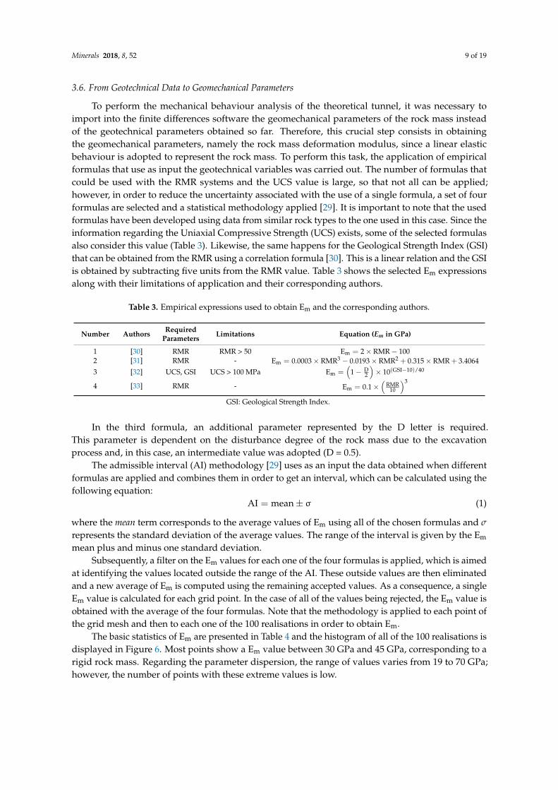
The basic statistics of Em are presented in Table 4 and the histogram of all of the 100 realisations isdisplayed in Figure 6. Most points show a Em value between 30 GPa and 45 GPa, corresponding to arigid rock mass. Regarding the parameter dispersion, the range of values varies from 19 to 70 GPa;however, the number of points with these extreme values is low.

Minerals 2018, 8, 52 10 of 19
Table 4. Statistical analysis of the Em (in GPa) values obtained through the application of empiricalformulae using the geotechnical information.
Statistical Parameter Em (in GPa)
Total of points with information 100,800Mean 39.50
Variance 7.30Standard deviation 2.70
Minimum 19.74Maximum 71.53
Minerals 2018, 8, x FOR PEER REVIEW 10 of 19
Table 4. Statistical analysis of the Em (in GPa) values obtained through the application of empirical formulae using the geotechnical information.
Statistical Parameter 𝐄𝐄𝐦𝐦 (in GPa) Total of points with
information 100,800
Mean 39.50 Variance 7.30
Standard deviation 2.70 Minimum 19.74 Maximum 71.53
Figure 6 Histograms of the Em values (in GPa) obtained for all of the 100 realisations (each colour represents one realisation).
3.7. Scenario Reduction
As a first step, the 100 realisations of the rock mass deformation modulus, obtained using geostatistical simulation, are represented in a 2D space using the Euclidean distance as a metric (Figure 7). In order to apply the kernel algorithm, the Euclidean space should be transformed to a more linear space, the Feature Space. This intermediate stage can be achieved through the application of the kernel algorithm with a bandwidth of approximately 20% of the maximum Euclidean distance. To choose the optimal number of clusters, a silhouette average width test is performed [26]. This test allows for an assessment of the number of clusters that best represents the overall group of realisations and is performed from 2 until 10 clusters (i.e., the maximum number of clusters is predefined as 10). In this case, the optimal number of clusters is 4, which, from a geotechnical point of view, should be enough to cover the more conservative, the intermediate, and the optimistic scenarios. The final division into four clusters is obtained after applying kernel k-medoid clustering, which was run 500 times. Figure 7b displays the resulting configuration, where each cluster medoid is identified with a square and the corresponding elements with points in the same colour.
In order to confirm that the selected realisations statistically represent the full set, a validation is performed based on the comparison between the results for percentiles 10, 50, and 90 for all of the realisations. These percentiles are computed for each point of the grid point and then are averaged over the grid points. In this way, it is possible to obtain a single (average) value to represent each percentile (10, 50, and 90). Secondly, the percentiles 10, 50, and 90 computed for each grid point are summed point-by-point in order to understand the percentile trend for each realisation set. From Figure 8, it is possible to verify that, for a four-cluster configuration, the correspondence between the
Figure 6. Histograms of the Em values (in GPa) obtained for all of the 100 realisations (each colourrepresents one realisation).
3.7. Scenario Reduction
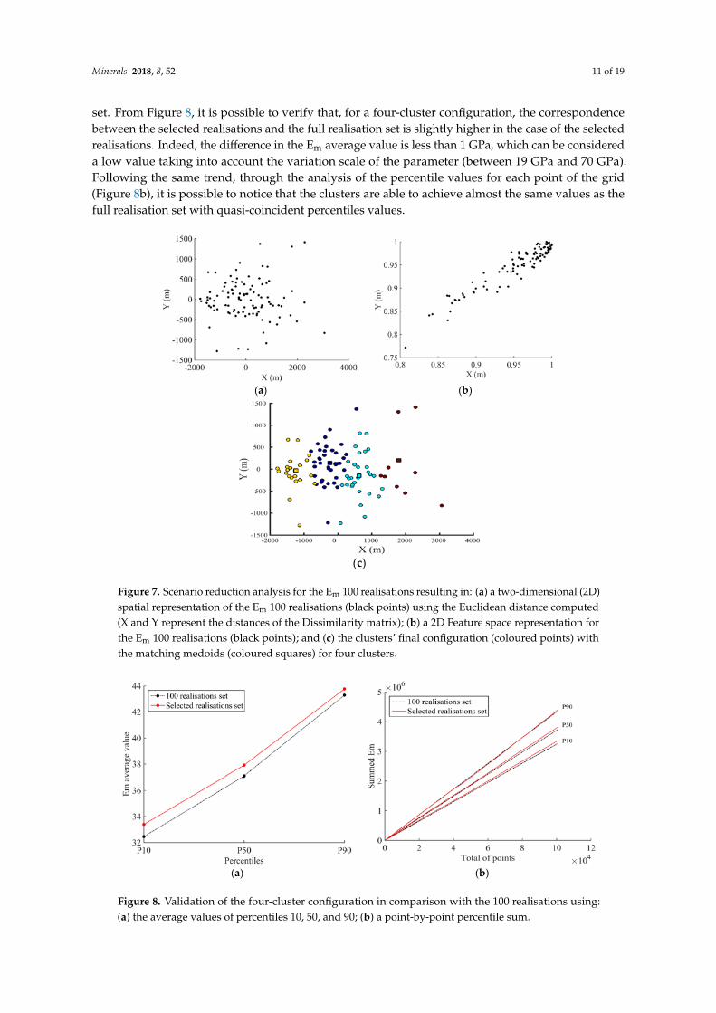
As a first step, the 100 realisations of the rock mass deformation modulus, obtained usinggeostatistical simulation, are represented in a 2D space using the Euclidean distance as a metric(Figure 7). In order to apply the kernel algorithm, the Euclidean space should be transformed to amore linear space, the Feature Space. This intermediate stage can be achieved through the applicationof the kernel algorithm with a bandwidth of approximately 20% of the maximum Euclidean distance.To choose the optimal number of clusters, a silhouette average width test is performed [26]. This testallows for an assessment of the number of clusters that best represents the overall group of realisationsand is performed from 2 until 10 clusters (i.e., the maximum number of clusters is predefined as 10).In this case, the optimal number of clusters is 4, which, from a geotechnical point of view, shouldbe enough to cover the more conservative, the intermediate, and the optimistic scenarios. The finaldivision into four clusters is obtained after applying kernel k-medoid clustering, which was run500 times. Figure 7b displays the resulting configuration, where each cluster medoid is identified witha square and the corresponding elements with points in the same colour.
In order to confirm that the selected realisations statistically represent the full set, a validationis performed based on the comparison between the results for percentiles 10, 50, and 90 for allof the realisations. These percentiles are computed for each point of the grid point and then areaveraged over the grid points. In this way, it is possible to obtain a single (average) value to representeach percentile (10, 50, and 90). Secondly, the percentiles 10, 50, and 90 computed for each gridpoint are summed point-by-point in order to understand the percentile trend for each realisation
Minerals 2018, 8, 52 11 of 19
set. From Figure 8, it is possible to verify that, for a four-cluster configuration, the correspondencebetween the selected realisations and the full realisation set is slightly higher in the case of the selectedrealisations. Indeed, the difference in the Em average value is less than 1 GPa, which can be considereda low value taking into account the variation scale of the parameter (between 19 GPa and 70 GPa).Following the same trend, through the analysis of the percentile values for each point of the grid(Figure 8b), it is possible to notice that the clusters are able to achieve almost the same values as thefull realisation set with quasi-coincident percentiles values.
Minerals 2018, 8, x FOR PEER REVIEW 11 of 19
selected realisations and the full realisation set is slightly higher in the case of the selected realisations. Indeed, the difference in the Em average value is less than 1 GPa, which can be considered a low value taking into account the variation scale of the parameter (between 19 GPa and 70 GPa). Following the same trend, through the analysis of the percentile values for each point of the grid (Figure 8b), it is possible to notice that the clusters are able to achieve almost the same values as the full realisation set with quasi-coincident percentiles values.
(a) (b)
(c)
Figure 7. Scenario reduction analysis for the Em 100 realisations resulting in: (a) a two-dimensional (2D) spatial representation of the Em 100 realisations (black points) using the Euclidean distance computed (X and Y represent the distances of the Dissimilarity matrix); (b) a 2D Feature space representation for the Em 100 realisations (black points); and (c) the clusters’ final configuration (coloured points) with the matching medoids (coloured squares) for four clusters.
(a) (b)
Figure 8. Validation of the four-cluster configuration in comparison with the 100 realisations using: (a) the average values of percentiles 10, 50, and 90; (b) a point-by-point percentile sum.
Figure 7. Scenario reduction analysis for the Em 100 realisations resulting in: (a) a two-dimensional (2D)spatial representation of the Em 100 realisations (black points) using the Euclidean distance computed(X and Y represent the distances of the Dissimilarity matrix); (b) a 2D Feature space representation forthe Em 100 realisations (black points); and (c) the clusters’ final configuration (coloured points) withthe matching medoids (coloured squares) for four clusters.
Minerals 2018, 8, x FOR PEER REVIEW 11 of 19
selected realisations and the full realisation set is slightly higher in the case of the selected realisations. Indeed, the difference in the Em average value is less than 1 GPa, which can be considered a low value taking into account the variation scale of the parameter (between 19 GPa and 70 GPa). Following the same trend, through the analysis of the percentile values for each point of the grid (Figure 8b), it is possible to notice that the clusters are able to achieve almost the same values as the full realisation set with quasi-coincident percentiles values.
(a) (b)
(c)
Figure 7. Scenario reduction analysis for the Em 100 realisations resulting in: (a) a two-dimensional (2D) spatial representation of the Em 100 realisations (black points) using the Euclidean distance computed (X and Y represent the distances of the Dissimilarity matrix); (b) a 2D Feature space representation for the Em 100 realisations (black points); and (c) the clusters’ final configuration (coloured points) with the matching medoids (coloured squares) for four clusters.
(a) (b)
Figure 8. Validation of the four-cluster configuration in comparison with the 100 realisations using: (a) the average values of percentiles 10, 50, and 90; (b) a point-by-point percentile sum.
Figure 8. Validation of the four-cluster configuration in comparison with the 100 realisations using:(a) the average values of percentiles 10, 50, and 90; (b) a point-by-point percentile sum.

Minerals 2018, 8, 52 12 of 19
4. Numerical Modelling Results
In order to understand the advantages of using the proposed methodology, the numerical modelsresulting from the individual realisations are compared with a deterministic approach, which considersthe rock mass as a homogeneous medium (deterministic values for the geomechanical parameters).Therefore, for the deterministic model, here referred to as model 1, the rock mass deformationmodulus is obtained firstly by averaging the RMR values in all of the 100,800 zone centroids and,subsequently, by applying the four aforementioned empirical formulas and averaging the Em results.Likewise, a model referred to as model 2 contemplates the four medoids (individual realisations)selected after applying the scenario reduction explained above. Finally, and since the computationaltime of each model is modest due to the simplicity of the theoretical tunnel, the results from theprevious models are compared with the ones obtained for each one of the 100 realisations. It isimportant to point out that this analysis will also serve as a validation for the scenario reductionmethodology and, subsequently, for the proposed approach.
For the sake of clarification for all of the analysed models, Figure 9 presents a scheme illustratingthe path followed on the mentioned process, starting with the variable selection and its geostatisticalsimulation, then the application of the scenario reduction methodology, and finally the Em outputvalues. Regarding model 1, the deterministic value adopted to represent Em is 32.73 GPa.
Minerals 2018, 8, x FOR PEER REVIEW 12 of 19
4. Numerical Modelling Results
In order to understand the advantages of using the proposed methodology, the numerical models resulting from the individual realisations are compared with a deterministic approach, which considers the rock mass as a homogeneous medium (deterministic values for the geomechanical parameters). Therefore, for the deterministic model, here referred to as model 1, the rock mass deformation modulus is obtained firstly by averaging the RMR values in all of the 100,800 zone centroids and, subsequently, by applying the four aforementioned empirical formulas and averaging the Em results. Likewise, a model referred to as model 2 contemplates the four medoids (individual realisations) selected after applying the scenario reduction explained above. Finally, and since the computational time of each model is modest due to the simplicity of the theoretical tunnel, the results from the previous models are compared with the ones obtained for each one of the 100 realisations. It is important to point out that this analysis will also serve as a validation for the scenario reduction methodology and, subsequently, for the proposed approach.
For the sake of clarification for all of the analysed models, Figure 9 presents a scheme illustrating the path followed on the mentioned process, starting with the variable selection and its geostatistical simulation, then the application of the scenario reduction methodology, and finally the Em output values. Regarding model 1, the deterministic value adopted to represent Em is 32.73 GPa.
Figure 9. Workflow applied to build the different models to represent the rock mass characterisation of the rock mass using as an input the RMR system.
In this section, the numerical results obtained from the finite difference calculations are presented. Emphasis will be given to the results in terms of displacements, since the deformation modulus affects them in a direct way; however, some reference will be made to the maximum and minimum principal stress values calculated in the rock mass. This analysis is performed for all of the mentioned models. In detail, regarding the displacements on the rock mass, the maximum values obtained on the top of the tunnel arch, at the mid-point of the invert and at mid-height on the left and right sidewalls, are registered.
Primarily, Table 5 presents a summary of the maximum, minimum, and percentile values obtained from the calculations for the 100 individual realisations. Since model 2 concerns individual
Figure 9. Workflow applied to build the different models to represent the rock mass characterisation ofthe rock mass using as an input the RMR system.
In this section, the numerical results obtained from the finite difference calculations are presented.Emphasis will be given to the results in terms of displacements, since the deformation modulus affectsthem in a direct way; however, some reference will be made to the maximum and minimum principalstress values calculated in the rock mass. This analysis is performed for all of the mentioned models.In detail, regarding the displacements on the rock mass, the maximum values obtained on the topof the tunnel arch, at the mid-point of the invert and at mid-height on the left and right sidewalls,are registered.
Primarily, Table 5 presents a summary of the maximum, minimum, and percentile values obtainedfrom the calculations for the 100 individual realisations. Since model 2 concerns individual realisations,they are also included in the 100 realisations values. Note that these values should serve as a referencefor further comparisons.

Minerals 2018, 8, 52 13 of 19
Table 5. Displacements and stresses values obtained for the 100 individual realisations.
StatisticalParameter
Vertical Displacement (mm) HorizontalDisplacement (mm) Max. Stress
(MPa)Min. Stress
(MPa)Arch Invert Left Wall Right Wall
Minimum 5.20 6.82 1.50 1.42 6.67 1.77Maximum 8.34 11.31 2.75 2.63 7.91 1.84
Mean 6.60 8.62 2.00 2.00 6.97 1.80P10 5.92 7.76 1.73 1.71 6.81 1.77P50 6.60 8.62 2.00 2.00 6.97 1.79P90 7.49 9.80 2.28 2.33 7.21 1.82
Comparing the 100 realisations results, some differences are worthy of reference, namely thedifferences between the maximum and minimum values for the vertical and horizontal displacements,where a significant range of values is obtained. In terms of principal stresses, these differences aresubtler with variations smaller than 1 MPa. Regarding the displacements’ mean values, the differencesbetween the left and right sidewalls are zero, confirming that the heterogeneities present in this rockmass are small.
Looking in detail at models 1 and 2, Table 6 shows a summary of the displacements andstresses obtained from the numerical analysis. Likewise, in order to understand the full data setrepresentation using the clusters, an individual analysis is completed for each displacement and stressvalue. The aim is to represent the maximum and minimum values of all of the analysed models.Therefore, in Figures 10 and 11, all of the model values for the displacements and principal stressesobtained after the tunnel excavation are represented.
Table 6. Summary of the displacements and stresses results obtained in models 1 and 2.
Model CorrespondingRealisation
VerticalDisplacement (mm)
HorizontalDisplacement (mm)
Max. Stress(MPa)
Arch Invert Left Wall Right Wall Arch Invert
Model 1 - 5.86 9.36 1.79 1.79 6.91 1.77Model 2-Cluster 1 Realisation 28 6.31 9.25 2.00 2.14 6.85 1.80Model 2-Cluster 2 Realisation 46 6.07 8.24 1.82 1.87 7.05 1.80Model 2-Cluster 3 Realisation 53 6.95 10.1 2.11 2.22 6.99 1.80Model 2-Cluster 4 Realisation 74 6.02 7.03 1.56 1.84 7.91 1.80
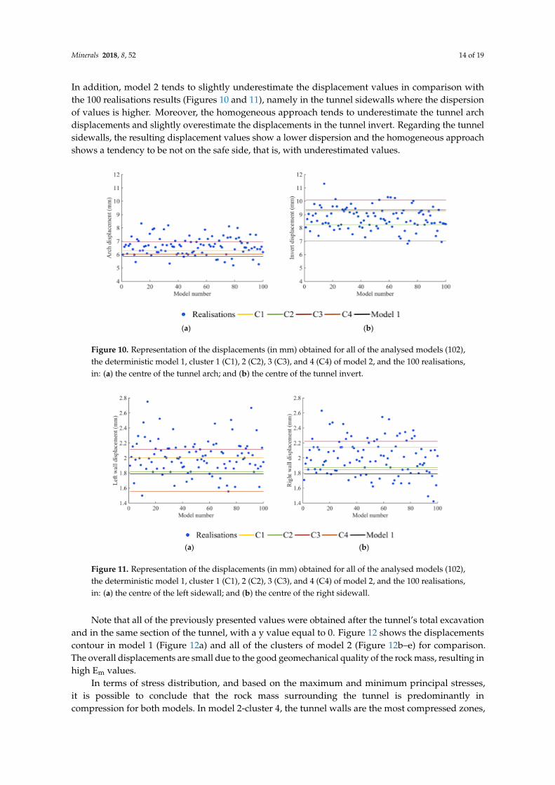
In what concerns the maximum displacements results, in a more general analysis, the followingcomments can be made: (1) there are significant differences between the displacements’ maximumvalues from cluster to cluster, mainly in the tunnel invert; (2) differences are registered in the horizontaldisplacements of the tunnel sidewalls; and (3) model 1 (homogeneous approach) shows, in general,lower displacement values in comparison with each individual cluster.
In a detailed analysis, the maximum vertical displacements of model 1 (homogeneous approach)are observed in the centre of the tunnel invert with a magnitude of 9.36 mm, while the central point ofthe tunnel arch shows a smaller value of 5.86 mm (Figure 10).
Concerning model 2, cluster 3 is the one that registers the highest displacement values in all of theanalysed points, while cluster 4 registers the lowest ones. The maximum vertical displacementoccurs in the centre of the tunnel invert with, approximately, 10.1 mm (cluster 3), whereas themaximum displacement on the tunnel arch admits a magnitude of 6.95 mm (cluster 3). For thesidewalls, the values vary between 1.56 mm (left) and 1.84 mm (right) for cluster number 4 and2.11 mm (left) and 2.22 mm (right) for cluster number 3. The observed disparity between thehorizontal displacements can be explained by the assumed variability in the Em values (Figure 11).Looking at Figures 10 and 11, it is possible to conclude that there are higher values and moredispersion in the displacements obtained in the tunnel invert in comparison with the tunnel arch.
Minerals 2018, 8, 52 14 of 19
In addition, model 2 tends to slightly underestimate the displacement values in comparison withthe 100 realisations results (Figures 10 and 11), namely in the tunnel sidewalls where the dispersionof values is higher. Moreover, the homogeneous approach tends to underestimate the tunnel archdisplacements and slightly overestimate the displacements in the tunnel invert. Regarding the tunnelsidewalls, the resulting displacement values show a lower dispersion and the homogeneous approachshows a tendency to be not on the safe side, that is, with underestimated values.
Minerals 2018, 8, x FOR PEER REVIEW 14 of 19
Looking at Figures 10 and 11, it is possible to conclude that there are higher values and more dispersion in the displacements obtained in the tunnel invert in comparison with the tunnel arch. In addition, model 2 tends to slightly underestimate the displacement values in comparison with the 100 realisations results (Figures 10 and 11), namely in the tunnel sidewalls where the dispersion of values is higher. Moreover, the homogeneous approach tends to underestimate the tunnel arch displacements and slightly overestimate the displacements in the tunnel invert. Regarding the tunnel sidewalls, the resulting displacement values show a lower dispersion and the homogeneous approach shows a tendency to be not on the safe side, that is, with underestimated values.
(a) (b)
Figure 10. Representation of the displacements (in mm) obtained for all of the analysed models (102), the deterministic model 1, cluster 1 (C1), 2 (C2), 3 (C3), and 4 (C4) of model 2, and the 100 realisations, in: (a) the centre of the tunnel arch; and (b) the centre of the tunnel invert.
(a) (b)
Figure 11. Representation of the displacements (in mm) obtained for all of the analysed models (102), the deterministic model 1, cluster 1 (C1), 2 (C2), 3 (C3), and 4 (C4) of model 2, and the 100 realisations, in: (a) the centre of the left sidewall; and (b) the centre of the right sidewall.
Note that all of the previously presented values were obtained after the tunnel’s total excavation and in the same section of the tunnel, with a y value equal to 0. Figure 12 shows the displacements contour in model 1 (Figure 12a) and all of the clusters of model 2 (Figure 12b–e) for comparison. The overall displacements are small due to the good geomechanical quality of the rock mass, resulting in high Em values.
In terms of stress distribution, and based on the maximum and minimum principal stresses, it is possible to conclude that the rock mass surrounding the tunnel is predominantly in compression for both models. In model 2-cluster 4, the tunnel walls are the most compressed zones, with values of 7.9
Figure 10. Representation of the displacements (in mm) obtained for all of the analysed models (102),the deterministic model 1, cluster 1 (C1), 2 (C2), 3 (C3), and 4 (C4) of model 2, and the 100 realisations,in: (a) the centre of the tunnel arch; and (b) the centre of the tunnel invert.
Minerals 2018, 8, x FOR PEER REVIEW 14 of 19
Looking at Figures 10 and 11, it is possible to conclude that there are higher values and more dispersion in the displacements obtained in the tunnel invert in comparison with the tunnel arch. In addition, model 2 tends to slightly underestimate the displacement values in comparison with the 100 realisations results (Figures 10 and 11), namely in the tunnel sidewalls where the dispersion of values is higher. Moreover, the homogeneous approach tends to underestimate the tunnel arch displacements and slightly overestimate the displacements in the tunnel invert. Regarding the tunnel sidewalls, the resulting displacement values show a lower dispersion and the homogeneous approach shows a tendency to be not on the safe side, that is, with underestimated values.
(a) (b)
Figure 10. Representation of the displacements (in mm) obtained for all of the analysed models (102), the deterministic model 1, cluster 1 (C1), 2 (C2), 3 (C3), and 4 (C4) of model 2, and the 100 realisations, in: (a) the centre of the tunnel arch; and (b) the centre of the tunnel invert.
(a) (b)
Figure 11. Representation of the displacements (in mm) obtained for all of the analysed models (102), the deterministic model 1, cluster 1 (C1), 2 (C2), 3 (C3), and 4 (C4) of model 2, and the 100 realisations, in: (a) the centre of the left sidewall; and (b) the centre of the right sidewall.
Note that all of the previously presented values were obtained after the tunnel’s total excavation and in the same section of the tunnel, with a y value equal to 0. Figure 12 shows the displacements contour in model 1 (Figure 12a) and all of the clusters of model 2 (Figure 12b–e) for comparison. The overall displacements are small due to the good geomechanical quality of the rock mass, resulting in high Em values.
In terms of stress distribution, and based on the maximum and minimum principal stresses, it is possible to conclude that the rock mass surrounding the tunnel is predominantly in compression for both models. In model 2-cluster 4, the tunnel walls are the most compressed zones, with values of 7.9
Figure 11. Representation of the displacements (in mm) obtained for all of the analysed models (102),the deterministic model 1, cluster 1 (C1), 2 (C2), 3 (C3), and 4 (C4) of model 2, and the 100 realisations,in: (a) the centre of the left sidewall; and (b) the centre of the right sidewall.
Note that all of the previously presented values were obtained after the tunnel’s total excavationand in the same section of the tunnel, with a y value equal to 0. Figure 12 shows the displacementscontour in model 1 (Figure 12a) and all of the clusters of model 2 (Figure 12b–e) for comparison.The overall displacements are small due to the good geomechanical quality of the rock mass, resulting inhigh Em values.
In terms of stress distribution, and based on the maximum and minimum principal stresses,it is possible to conclude that the rock mass surrounding the tunnel is predominantly incompression for both models. In model 2-cluster 4, the tunnel walls are the most compressed zones,

Minerals 2018, 8, 52 15 of 19
with values of 7.9 MPa and 1.8 MPa for the maximum and minimum principal stresses, respectively.Moreover, the tunnel arch and invert show compression stresses ranging between 4.0 MPa and 0.4 MPa.Similarly, the stresses of model 1 present the same range of values as model 2. Indeed, this similarity inthe stress values can be justified by the lower influence of the Em variation on the rock mass principalstresses. As expected, the stresses are smaller on the tunnel invert and arch where the maximumdisplacements are observed. Regarding the tensile stresses, they only appear in the centre of the wallsand invert with values under 0.2 MPa.
Minerals 2018, 8, x FOR PEER REVIEW 15 of 19
MPa and 1.8 MPa for the maximum and minimum principal stresses, respectively. Moreover, the tunnel arch and invert show compression stresses ranging between 4.0 MPa and 0.4 MPa. Similarly, the stresses of model 1 present the same range of values as model 2. Indeed, this similarity in the stress values can be justified by the lower influence of the Em variation on the rock mass principal stresses. As expected, the stresses are smaller on the tunnel invert and arch where the maximum displacements are observed. Regarding the tensile stresses, they only appear in the centre of the walls and invert with values under 0.2 MPa.
(a) (b)
(c) (d)
(e)
Figure 12. XZ plane at y = 0 with the contour of displacement (colour scale in m) of the rock mass after the excavation for: (a) model 1; (b) model 2-cluster 1; (c) model 2-cluster 2; (d) model 2-cluster 3; and (e) model 2-cluster 4.
5. Discussion
Figure 12. XZ plane at y = 0 with the contour of displacement (colour scale in m) of the rock massafter the excavation for: (a) model 1; (b) model 2-cluster 1; (c) model 2-cluster 2; (d) model 2-cluster 3;and (e) model 2-cluster 4.
5. Discussion
In this section, an analysis will be made comparing the obtained values for the displacementsand principal stresses of this tunnel case, with the aim to address three main points: (1) the

Minerals 2018, 8, 52 16 of 19
heterogeneity representation of the individual realisations when compared with a traditional approachthat assumes the rock mass is a homogeneous medium; (2) comparing the results, in terms of valuesand computational time, of using the scenario reduction optimal cluster configuration with respect toall of the 100 realisations, i.e., giving an answer to the question if the optimal clusters configuration isable to integrate the most conservative and optimistic values and embody a good solution to integrateinto the numerical analysis; and (3) the computational time needed to analyse the 100 geostatisticalrealisations and the ones obtained from the proposed methodology.
Regarding the first point, it is possible to observe from Figure 12 that the heterogeneity ofthe rock mass is manifested by the asymmetrical pattern of the displacements contour in model 2.Indeed, the disparity of the values of the horizontal displacements confirms this statement. In relationto model 1, model 2 shows percentage differences in displacements values ranging from 1% to 25%,being either positive or negative. In terms of principal stresses, the maximum difference between theheterogeneous (model 2) and the homogeneous approach was 14% for the maximum principal stressesand 2% in the case of the minimum principal stresses.
It seems important to mention that, even if they are small, the differences between a heterogeneousand a homogeneous model can be relevant in the geotechnical analysis of underground works; in fact,these differences should be higher as the rock mass spatial variability increases and as the rock massshows worse characteristics.
To perform the analysis regarding point number 2, histograms containing all the models’results have been computed (Figures 13 and 14). Similar to the graphical representation of thedisplacements and principal stress values, using the histograms it is possible to confirm the sametendency observed for model 2; that is, the ability of the model, introducing the concept of clustering,to show more optimistic and more conservative results. Also, it is possible to state that many of the100 realisations show values in-between the referred clusters, confirming the capability of the scenarioreduction methodology to represent, statistically, the full set of realisations. To complete this analysis,the first three moments (mean, standard deviation, and skewness) obtained from the 100 realisationsdistribution fitting can be consulted in Table 7. For all of the analysed zones, the displacementsshow a symmetrical distribution with some tendency to the right side (positive skewness); that is,higher displacements. About the third point concerning computational time, it was approximately2 h for each individual realisation. Hence, to analyse the 100 realisations a total of 200 h isneeded. If a reduction methodology is adopted, the time can go down to a maximum of 21 h(2 h per realisation for a maximum of 10 realisations, plus 1 h to apply the scenario reductionmethodology). However, we strongly believe that this time difference can even be bigger in the case ofmore complex numerical models that require more computational time in the finite difference software.
Minerals 2018, 8, x FOR PEER REVIEW 16 of 19
In this section, an analysis will be made comparing the obtained values for the displacements and principal stresses of this tunnel case, with the aim to address three main points: (1) the heterogeneity representation of the individual realisations when compared with a traditional approach that assumes the rock mass is a homogeneous medium; (2) comparing the results, in terms of values and computational time, of using the scenario reduction optimal cluster configuration with respect to all of the 100 realisations, i.e., giving an answer to the question if the optimal clusters configuration is able to integrate the most conservative and optimistic values and embody a good solution to integrate into the numerical analysis; and (3) the computational time needed to analyse the 100 geostatistical realisations and the ones obtained from the proposed methodology.
Regarding the first point, it is possible to observe from Figure 12 that the heterogeneity of the rock mass is manifested by the asymmetrical pattern of the displacements contour in model 2. Indeed, the disparity of the values of the horizontal displacements confirms this statement. In relation to model 1, model 2 shows percentage differences in displacements values ranging from 1% to 25%, being either positive or negative. In terms of principal stresses, the maximum difference between the heterogeneous (model 2) and the homogeneous approach was 14% for the maximum principal stresses and 2% in the case of the minimum principal stresses.
It seems important to mention that, even if they are small, the differences between a heterogeneous and a homogeneous model can be relevant in the geotechnical analysis of underground works; in fact, these differences should be higher as the rock mass spatial variability increases and as the rock mass shows worse characteristics.
To perform the analysis regarding point number 2, histograms containing all the models’ results have been computed (Figures 13 and 14). Similar to the graphical representation of the displacements and principal stress values, using the histograms it is possible to confirm the same tendency observed for model 2; that is, the ability of the model, introducing the concept of clustering, to show more optimistic and more conservative results. Also, it is possible to state that many of the 100 realisations show values in-between the referred clusters, confirming the capability of the scenario reduction methodology to represent, statistically, the full set of realisations. To complete this analysis, the first three moments (mean, standard deviation, and skewness) obtained from the 100 realisations distribution fitting can be consulted in Table 7. For all of the analysed zones, the displacements show a symmetrical distribution with some tendency to the right side (positive skewness); that is, higher displacements. About the third point concerning computational time, it was approximately 2 h for each individual realisation. Hence, to analyse the 100 realisations a total of 200 h is needed. If a reduction methodology is adopted, the time can go down to a maximum of 21 h (2 h per realisation for a maximum of 10 realisations, plus 1 h to apply the scenario reduction methodology). However, we strongly believe that this time difference can even be bigger in the case of more complex numerical models that require more computational time in the finite difference software.
(a) (b)
Figure 13. Histograms and distribution fitting curve for the 100 realisations and values (lines) for models 1 to 5 of displacements in: (a) the centre of the tunnel arch; (b) the centre of the tunnel invert. Figure 13. Histograms and distribution fitting curve for the 100 realisations and values (lines) for
models 1 to 5 of displacements in: (a) the centre of the tunnel arch; (b) the centre of the tunnel invert.

Minerals 2018, 8, 52 17 of 19Minerals 2018, 8, x FOR PEER REVIEW 17 of 19
(a) (b)
Figure 14. Histograms and distribution fitting curve for the 100 realisations and values (lines) for models 1 to 5 values (lines) of displacements in: (a) the centre of the left sidewall; (b) the centre of the right sidewall.
Table 7. Distribution curve fitting details (first three moments) regarding the 100 realisations’ obtained values for displacements.
Displacement Mean Standard Deviation
Skewness
Maximum horizontal displacement (mm): left sidewall 2.01 0.67 0.091 Maximum horizontal displacement (mm): right sidewall 2.00 0.24 0.100 Maximum vertical displacement (mm): centre of the arch 6.63 0.67 0.006 Maximum vertical displacement (mm): centre of the invert 8.71 0.83 0.003
6. Conclusions
In this work, a methodology for the numerical modelling of heterogeneous rock masses that considers uncertainty quantification, variability of the geomechanical parameters, and the presence of heterogeneities was presented. The methodology is outlined to combine geostatistical simulation and finite difference analysis. Therefore, using geotechnical information commonly obtained from field surveys, it is possible to simulate the variables of interest while honouring the values observed or measured at the data locations. A scenario reduction methodology allows researchers to obtain a smaller number of realisations without losing relevant information so that a numerical analysis of the underground structure can be made using a smaller number of possible scenarios. A prior step requires the conversion of the geotechnical information into the deformation modulus (Em) through the use of empirical formulas. If detailed in situ data based on large-scale tests existed, this step could be avoided.
In order to validate the proposed methodology, a real data set containing geotechnical data about a gold deposit was used. The geotechnical set contains information of the empirical system RMR and values of the UCS measured by laboratory tests. The main goal of this work was not only to validate the proposed methodology, but also to compare the main differences in the mechanical behaviour of the structure when modelled using the heterogeneous approach and a deterministic, i.e., an isotropic and homogeneous, model. The heterogeneous approach proved to be encouraging for heterogeneous rock mass modelling due to the lower computational time required and the capability to statistically represent a full set of realisations (resulting in different scenarios, from conservative to optimistic ones).
Therefore, the main findings of this work are: (1) the developed methodology allows for the simulation of a rock mass’s geomechanical properties and the export of that information into numerical analysis software to perform a rock mass mechanical behaviour analysis; (2) the use of geostatistical information allows for the identification of a rock mass’s spatial variability and
Figure 14. Histograms and distribution fitting curve for the 100 realisations and values (lines) formodels 1 to 5 values (lines) of displacements in: (a) the centre of the left sidewall; (b) the centre of theright sidewall.
Table 7. Distribution curve fitting details (first three moments) regarding the 100 realisations’ obtainedvalues for displacements.
Displacement Mean Standard Deviation Skewness
Maximum horizontal displacement (mm): left sidewall 2.01 0.67 0.091Maximum horizontal displacement (mm): right sidewall 2.00 0.24 0.100Maximum vertical displacement (mm): centre of the arch 6.63 0.67 0.006Maximum vertical displacement (mm): centre of the invert 8.71 0.83 0.003
6. Conclusions
In this work, a methodology for the numerical modelling of heterogeneous rock masses thatconsiders uncertainty quantification, variability of the geomechanical parameters, and the presenceof heterogeneities was presented. The methodology is outlined to combine geostatistical simulationand finite difference analysis. Therefore, using geotechnical information commonly obtained fromfield surveys, it is possible to simulate the variables of interest while honouring the values observedor measured at the data locations. A scenario reduction methodology allows researchers to obtain asmaller number of realisations without losing relevant information so that a numerical analysis ofthe underground structure can be made using a smaller number of possible scenarios. A prior steprequires the conversion of the geotechnical information into the deformation modulus (Em) throughthe use of empirical formulas. If detailed in situ data based on large-scale tests existed, this step couldbe avoided.
In order to validate the proposed methodology, a real data set containing geotechnical data abouta gold deposit was used. The geotechnical set contains information of the empirical system RMR andvalues of the UCS measured by laboratory tests. The main goal of this work was not only to validatethe proposed methodology, but also to compare the main differences in the mechanical behaviour ofthe structure when modelled using the heterogeneous approach and a deterministic, i.e., an isotropicand homogeneous, model. The heterogeneous approach proved to be encouraging for heterogeneousrock mass modelling due to the lower computational time required and the capability to statisticallyrepresent a full set of realisations (resulting in different scenarios, from conservative to optimistic ones).
Therefore, the main findings of this work are: (1) the developed methodology allows for thesimulation of a rock mass’s geomechanical properties and the export of that information into numericalanalysis software to perform a rock mass mechanical behaviour analysis; (2) the use of geostatistical

Minerals 2018, 8, 52 18 of 19
information allows for the identification of a rock mass’s spatial variability and heterogeneities,which results in more accurate and realistic rock mass models; (3) although the rock mass used herehad lower variability, some interesting differences were detected between the proposed approachand the homogeneous one, with the homogeneous one having a tendency to underestimate thedisplacement value (which is not on the safe side); and (4) the scenario reduction methodology allowsresearchers to obtain a reduced and practical number of realisations that produces results that arerepresentative of the full realisations set.
In future developments, the proposed methodology should be validated with a different type ofrock where the geomechanical variability is higher.
Acknowledgments: This research work has been developed in the scope of the Doctoral Programme inCivil Engineering at the University of Minho, Portugal. It was supported by the Portuguese Science andTechnology Foundation (FCT), under grant No. SFRH/BD/89627/2012 inserted in the LNEC project namedP2I-RockGeoStat, and by the Chilean Commission for Scientific and Technological Research, under grantCONICYT/FONDECYT/REGULAR/N◦1170101.
Author Contributions: Marisa Pinheiro, Xavier Emery, Tiago Miranda, Luís Lamas, and Margarida Espadaconceived and designed the experiments; Marisa Pinheiro performed the experiments; and Marisa Pinheiro andXavier Emery wrote the paper.
Conflicts of Interest: The authors declare no conflict of interest. The founding sponsors had no role in the designof the study; in the collection, analyses, or interpretation of data; in the writing of the manuscript, and in thedecision to publish the results.
References
1. Metropolis, N.; Ulam, S. The monte carlo method. J. Am. Stat. Assoc. 1949, 44, 335–341. [CrossRef] [PubMed]2. Ang, A.H.-S.; Tang, W.H. Probability Concepts in Engineering Planning and Design; John Wiley & Sons:
New York, NY, USA, 1984.3. Madani, N.; Asghari, O. Fault detection in 3D by sequential Gaussian simulation of Rock Quality Designation
(RQD). Arabian J. Geosci. 2013, 12, 3737–3747. [CrossRef]4. Ozturk, C.A.; Nasuf, E. Geostatistical assessment of rock zones for tunneling. Tunn. Undergr. Space Technol.
2002, 17, 275–285. [CrossRef]5. Ryu, D.W.; Kim, T.K.; Heo, J.S. A study on geostatistical simulation technique for the uncertainty modelling
of RMR. Tunn. Undergr. 2003, 13, 87–99.6. You, K.H. An estimation technique of rock mass classes for a tunnel design. Geotech. Eng. 2003, 19, 319–326.
(In Korean)7. Oh, S.; Chung, H.; Kee Lee, D. Geostatistical integration of MT and boreholes data for RMR evaluation.
Environ. Geol. 2004, 46, 1070–1078. [CrossRef]8. Stavropoulou, M.; Exadaktylos, G.; Saratsis, G. A combined three-dimensional geological-geostatistical
numerical model of underground excavations in rock. Rock Mech. Rock Eng. 2007, 40, 213–243. [CrossRef]9. Exadaktylos, G.; Stavropoulou, M. A specific upscaling theory of rock mass parameters exhibiting spatial
variability: Analytical relations and computational scheme. Int. J. Rock Mech. Min. Sci. 2008, 45, 1102–1125.[CrossRef]
10. Jeon, S.; Hong, C.; You, K. Design of tunnel supporting system using geostatistical methods. In GeotechnicalAspects of Underground Construction in Soft Ground; Liu, H., Ed.; CRC Press: Boca Raton, FL, USA, 2009;pp. 781–784.
11. Egaña, M.; Ortiz, J. Assessment of RMR and its uncertainty by using geostatistical simulation in a miningproject. J. GeoEng. 2013, 8, 83–90.
12. Ferrari, F.; Apuani, T.; Giani, G.P. Rock Mass Rating spatial estimation by geostatistical analysis. Int. J. RockMech. Min. Sci. 2014, 70, 162–176. [CrossRef]
13. Ellefmo, S.L.; Eidsvik, J. Local and spatial 476 joint frequency uncertainty and its application to rock masscharacterisation. Rock Mech. Rock Eng. 2009, 42, 667–668. [CrossRef]
14. Ozturk, C.A.; Simdi, E. Geostatistical investigation of geotechnical and constructional properties inKadikoy–Kartal subway, Turkey. Tunn. Undergr. Space Technol. 2014, 4, 35–45. [CrossRef]

Minerals 2018, 8, 52 19 of 19
15. Deisman, N.; Khajeh, M.; Chalaturnyk, R.J. Using geological strength index (GSI) to model uncertainty inrock mass properties of coal for CBM/ECBM reservoir geomechanics. Int. J. Coal Geol. 2013, 112, 76–86.[CrossRef]
16. Pinheiro, M.; Emery, X.; Miranda, T.; Vallejos, J. Truncated Gaussian simulation to map the spatialheterogeneity of rock mass rating. Rock Mech. Rock Eng. 2016, 49, 1–6. [CrossRef]
17. Pinheiro, M.; Vallejos, J.; Miranda, T.; Emery, X. Geostatistical simulation to map the spatial heterogeneity ofgeomechanical parameters: A case study with rock mass rating. Eng. Geol. 2016, 205, 93–103. [CrossRef]
18. Chilès, J.P.; Delfiner, P. Geostatistics: Modeling Spatial Uncertainty; John Wiley & Sons: New York, NY, USA,2012; p. 699.
19. Scheidt, C.; Caers, J. Uncertainty quantification in reservoir performance using distances and Kernelmethods-application to a West Africa deep-water turbidite reservoir. SPE J. 2009, 14, 680–692. [CrossRef]
20. Scheidt, C.; Caers, J. Representing spatial uncertainty using distances and kernels. Math. Geosci. 2009, 41,397–419. [CrossRef]
21. Armstrong, M.; Ndiaye, A.; Razanatsimba, R.; Galli, A. Scenario reduction applied to geostatisticalsimulations. Math. Geosci. 2013, 45, 165–182. [CrossRef]
22. Deutsch, C.V.; Srinivasan, S. Improved reservoir management through ranking stochastic reservoir models.In Proceedings of the SPE/DOE Improved Oil Recovery Symposium’96, Tulsa, OK, USA, 21–24 April 1996.[CrossRef]
23. McLennan, J.A.; Deutsch, C.V. Ranking geostatistical realizations by measures connectivity. In Proceedingsof the SPE/PS-CIM/CHOA International Thermal Operations and Heavy Oil Symposium, Calgary, AB,Canada, 1–3 November 2005.
24. Itasca. FLAC—Fast Lagrangian Analysis of Continua 2013, Version 5.0 User’s Manual; Itasca Consulting Group,Inc.: Minneapolis, MN, USA, 2013.
25. Emery, X.; Lantuéjoul, C. TBSIM: A computer program for conditional simulation of three-dimensionalGaussian random fields via the turning bands method. Comput. Geosci. 2006, 32, 1615–1628. [CrossRef]
26. Tibshirani, R.; Walther, G.; Hastie, T. Estimating the number of clusters in a data set via the gap statistic. J. R.Stat. Soc. Ser. B 2001, 63, 411–423. [CrossRef]
27. Rousseeuw, P.J. Silhouettes: A graphical aid to the interpretation and validation of cluster analysis. J. Comput.Appl. Math. 1987, 20, 53–65. [CrossRef]
28. Bieniawski, Z.T. Engineering Rock Mass Classifications; John Wiley & Sons: New York, NY, USA, 1989; p. 272.29. Miranda, T. Contribution to the Calculation of Geomechanical Parameters for Underground Structures
Modelling in Granite Formations. Master’s Thesis, University of Minho, Guimarães, Portugal, 2003; p. 186.(In Portuguese)
30. Hoek, E.; Brown, E.T. Practical estimates of rock mass strength. Int. J. Rock Mech. Min. Sci. 1997, 34,1165–1186. [CrossRef]
31. Mohammadi, H.; Rahmannejad, R. The estimation of rock mass deformation modulus using regression andartificial neural network analysis. Arabian J. Sci. Eng. 2010, 1A, 205–217.
32. Hoek, E.; Carranza-Torres, C.; Corkum, B. Hoek-Brown failure criterion-2002 Edition. In Proceedings ofthe Fifth North American Rock Mechanics Symposium, Toronto, ON, Canada, 7–10 July 2002; Volume 1,pp. 267–273.
33. Read, S.A.L.; Perrin, N.D.; Richards, L.R. Applicability of the Hoek–Brown failure criterion to New Zealandgreywacke rocks. In Proceedings of the Ninth International Congress on Rock Mechanics, Paris, France,25–28 August 1999; Volume 2, pp. 655–660.
© 2018 by the authors. Licensee MDPI, Basel, Switzerland. This article is an open accessarticle distributed under the terms and conditions of the Creative Commons Attribution(CC BY) license (http://creativecommons.org/licenses/by/4.0/).