modelling and simulation of service area based ofdm air … · 2011-05-27 · yin liu...
TRANSCRIPT

Yin LiuKurt–Schumacher-Str. 46D–67663 KaiserslauternGebourtsort: Beijing/China
Modelling and Simulation of Service Area BasedOFDM Air Interfaces for Beyond 3G Mobile Radio
Systems
deutscher Titel:
Modellierung und Simulation vonOFDM–Luftschnittstellen fur Mobilfunksystemejenseits der dritten Generation auf der Basis von
Service–Gebieten
Vom Fachbereich Elektrotechnik und Informationstechnik
der Technischen Universitat Kaiserslautern
zur Verleihung des akademischen Grades
Doktor der Ingenieurwissenschaften (Dr.–Ing.)
genehmigte Dissertation
von
M.Sc. Yin Liu
D 386
Tag der Einreichung: 2. Dezember 2004Tag der mundlichen Prufung: 11. Februar 2005
Dekan des FachbereichsElektrotechnik: Prof. Dr.–Ing. G. Huth
Vorsitzender derPrufungskommission: Prof. Dr.–Ing. habil. A. Potchinkov
1. Berichterstatter: Prof. Dr.–Ing. habil. Dr.–Ing. E. h. P.W. Baier2. Berichterstatter: Prof. Dr.–Ing. R. Zengerle


III
Vorwort
Die vorliegende Arbeit entstand in der Zeit von November 2001 bis Februar 2005
im Rahmen meiner Tatigkeit als wissenschaftliche Mitarbeiterin Prof. Dr.–Ing. ha-
bil. Dr.–Ing. E. h. P. W. Baiers am Lehrstuhl fur hochfrequente Signalubertragung
und –verarbeitung der Technischen Universitat Kaiserslautern. Ich mochte all jenen
danken, die mich bei der Entstehung dieser Arbeit unterstutzt haben.
Mein besonderer Dank ergeht an Herrn Prof. Baier fur die Anregung, die Betreuung
und die Forderung meiner Arbeit. Durch seine stete Diskussionsbereitschaft sowie
durch zahlreiche Ratschlage und Hinweise hat er wesentlich zum Gelingen dieser Arbeit
beigetragen.
Herrn Prof. Dr.–Ing. R. Zengerle danke ich fur zahlreiche sehr hilfreiche Hinweise fur
die kritisch–kooperative Durchsicht der Dissertation und fur die Ubernahme des Ko-
rreferats. Weiterhin danke ich dem Vorsitzenden der Promotionskommission, Herrn
Prof. Dr.–Ing. habil. A. Potchinkov. Im Rahmen meiner wissenschaftlichen Arbeit
entstand auch eine enge Kooperation mit der Arbeitsgruppe Prof. Dr. H. Rohlings,
TU Hamburg-Harburg, aus der wichtige Anregungen und Hinweise fur meine Arbeit
resultierten.
Den jetzigen und den ehemaligen Kollegen am Lehrstuhl fur hochfrequente Signal–
ubertragung und –verarbeitung danke ich fur die angenehme Arbeitsatmosphare
und fur viele fruchtbare Diskussionen, die mir oftmals weitergeholfen haben. Ein
besonderer Dank ergeht an Herrn Dr.–Ing. habil. T. Weber fur die Betreuung und die
Unterstutzung beim Einarbeiten in das JOINT–Konzept und fur die freundschaftliche
Zusammenarbeit in gemeinsamen Projekten. Weiterhin bedanke ich mich herzlich bei
den Herren Dr.–Ing. A. Sklavos und Dr.–Ing. I. Maniatis fur die gute Zusammenarbeit.
Mein Dank gebuhrt auch der Siemens AG, insbesondere den Herren Dr.–Ing. E. Schulz
und Dipl.–Ing. W. Zirwas, fur die Forderung meiner Arbeit und viele fruchtbare Disku–
ssionen.
Der Technischen Universitat Kaiserslautern danke ich fur die Moglichkeit die
leistungsfahigen Rechner des Regionalen Hochschulrechenzentrums Kaiserslautern
(RHRK) zu benutzen. Den Mitarbeitern des RHRK danke ich fur die Beratung und
die Hilfestellung in Rechnerfragen.
Ein weiterer Dank ergeht an alle Studenten, die im Rahmen ihrer Studien–, Diplom–
und Masterarbeiten sowie als wissenschaftliche Hilfskrafte unter meiner Anleitung

IV
Beitrage zu dieser Arbeit geleistet haben.
Nicht zuletzt mochte ich mich bei meinem Mann Tao Tang und meiner Schwester Yi
Liu bedanken, die mir immer ein großer Ruckhalt waren. Ganz besonders herzlich
danke ich meiner Mutter Liqin Lin und meinem Vater Tonglin Liu. Sie haben mir
das Studium der Elektrotechnik ermoglicht und mich immer nach besten Kraften
unterstutzt. Ihnen ist diese Arbeit gewidmet.
Kaiserslautern, im Februar 2005
Yin Liu

V
Contents
1 Introduction 1
1.1 Service area based architectures versus cellular architectures . . . . . . 1
1.2 Basic features of JOINT as considered in the thesis . . . . . . . . . . . 4
1.3 Importance of modelling and simulation of JOINT . . . . . . . . . . . . 6
1.4 Open questions . . . . . . . . . . . . . . . . . . . . . . . . . . . . . . . 7
1.5 Goals and structure of the thesis . . . . . . . . . . . . . . . . . . . . . 8
2 Channel models 11
2.1 Preliminary remarks . . . . . . . . . . . . . . . . . . . . . . . . . . . . 11
2.2 Modelling in both time and frequency domains . . . . . . . . . . . . . . 11
2.3 Characteristics of the channel . . . . . . . . . . . . . . . . . . . . . . . 12
2.3.1 Fast fading . . . . . . . . . . . . . . . . . . . . . . . . . . . . . 12
2.3.2 Slow fading . . . . . . . . . . . . . . . . . . . . . . . . . . . . . 16
3 JOINT: A multipoint–to–multipoint OFDM system 20
3.1 Motivation . . . . . . . . . . . . . . . . . . . . . . . . . . . . . . . . . . 20
3.2 OFDM transmission technique . . . . . . . . . . . . . . . . . . . . . . . 20
3.3 Time synchronization . . . . . . . . . . . . . . . . . . . . . . . . . . . . 25
3.4 Parametrization of JOINT . . . . . . . . . . . . . . . . . . . . . . . . . 28
4 Maximum–likelihood joint channel estimation in the uplink of JOINT 31
4.1 Preliminary remarks . . . . . . . . . . . . . . . . . . . . . . . . . . . . 31
4.2 System model . . . . . . . . . . . . . . . . . . . . . . . . . . . . . . . . 31
4.3 Algorithm of joint channel estimation . . . . . . . . . . . . . . . . . . . 33
4.4 Choice of the pilot vectors . . . . . . . . . . . . . . . . . . . . . . . . . 34
5 Linear zero–forcing joint detection in the uplink of JOINT 36
5.1 Preliminary remarks . . . . . . . . . . . . . . . . . . . . . . . . . . . . 36
5.2 System model in the uplink of JOINT . . . . . . . . . . . . . . . . . . . 36
5.3 Algorithm of linear zero–forcing joint detection . . . . . . . . . . . . . . 38
5.3.1 Reference system: matched filter . . . . . . . . . . . . . . . . . 38
5.3.2 Zero forcing . . . . . . . . . . . . . . . . . . . . . . . . . . . . . 38
5.3.3 Signal–to–noise–ratio degradation . . . . . . . . . . . . . . . . . 39
6 Linear zero–forcing joint transmission in the downlink of JOINT 40
6.1 Preliminary remarks . . . . . . . . . . . . . . . . . . . . . . . . . . . . 40
6.2 System model in the downlink of JOINT . . . . . . . . . . . . . . . . . 40
6.3 Algorithm of linear zero–forcing joint transmission . . . . . . . . . . . . 43

VI Contents
6.3.1 Reference system: matched filter . . . . . . . . . . . . . . . . . 43
6.3.2 Transmit zero forcing . . . . . . . . . . . . . . . . . . . . . . . . 43
6.3.3 Transmission efficiency . . . . . . . . . . . . . . . . . . . . . . . 44
7 Implementation of the JOINT simulation chain 46
7.1 Preliminary remarks . . . . . . . . . . . . . . . . . . . . . . . . . . . . 46
7.2 Fundamentals of software engineering . . . . . . . . . . . . . . . . . . . 46
7.3 Introduction to MLDesigner . . . . . . . . . . . . . . . . . . . . . . . . 48
7.4 Implementation of key modules of the JOINT simulation chain . . . . . 50
7.4.1 Preliminary remarks . . . . . . . . . . . . . . . . . . . . . . . . 50
7.4.2 Channel models . . . . . . . . . . . . . . . . . . . . . . . . . . . 51
7.4.3 Joint channel estimation . . . . . . . . . . . . . . . . . . . . . . 54
7.4.4 Joint detection . . . . . . . . . . . . . . . . . . . . . . . . . . . 56
7.4.5 Joint transmission . . . . . . . . . . . . . . . . . . . . . . . . . 59
7.5 Implementation of the JOINT simulation chain . . . . . . . . . . . . . 62
7.6 Specific problems and solutions . . . . . . . . . . . . . . . . . . . . . . 64
7.6.1 Synchronization . . . . . . . . . . . . . . . . . . . . . . . . . . . 64
7.6.2 Simulation efficiency . . . . . . . . . . . . . . . . . . . . . . . . 65
8 Performance of JOINT in a single–service–area scenario 68
8.1 Preliminary remarks . . . . . . . . . . . . . . . . . . . . . . . . . . . . 68
8.2 Duality of the uplink and the downlink performances . . . . . . . . . . 68
8.2.1 General model of linear data transmission . . . . . . . . . . . . 68
8.2.2 Bit error probability . . . . . . . . . . . . . . . . . . . . . . . . 71
8.2.3 Energy efficiency . . . . . . . . . . . . . . . . . . . . . . . . . . 74
8.3 Impact of imperfect channel state information . . . . . . . . . . . . . . 76
8.3.1 Sources of imperfect channel state information . . . . . . . . . . 76
8.3.2 Impact of imperfect channel state information . . . . . . . . . . 80
8.4 Numerical results . . . . . . . . . . . . . . . . . . . . . . . . . . . . . . 87
8.4.1 Fixed channel snapshot . . . . . . . . . . . . . . . . . . . . . . . 87
8.4.2 Rayleigh fading channel . . . . . . . . . . . . . . . . . . . . . . 88
9 Performance of JOINT in a multiple–service–area scenario 92
9.1 Preliminary remarks . . . . . . . . . . . . . . . . . . . . . . . . . . . . 92
9.2 Multiple–service–area scenario . . . . . . . . . . . . . . . . . . . . . . . 92
9.3 Modified system model . . . . . . . . . . . . . . . . . . . . . . . . . . . 95
9.3.1 Uplink system model in a multiple–service–area scenario . . . . 95
9.3.2 Downlink system model in a multiple–service–area scenario . . . 96
9.4 Average bit error rate . . . . . . . . . . . . . . . . . . . . . . . . . . . . 98
9.5 Bit error rate statistics . . . . . . . . . . . . . . . . . . . . . . . . . . 103

Contents VII
9.6 Spectrum efficiency . . . . . . . . . . . . . . . . . . . . . . . . . . . . . 104
10 Summaries 109
10.1 English . . . . . . . . . . . . . . . . . . . . . . . . . . . . . . . . . . . . 109
10.2 Deutsch . . . . . . . . . . . . . . . . . . . . . . . . . . . . . . . . . . . 110
10.3 Chinese . . . . . . . . . . . . . . . . . . . . . . . . . . . . . . . . . . . 116
A Positions of access points and mobile terminals of Section 9.2 117
A.1 Preliminary remarks . . . . . . . . . . . . . . . . . . . . . . . . . . . . 117
A.2 Positions of access points . . . . . . . . . . . . . . . . . . . . . . . . . . 117
A.2.1 Positions of reference access points in co–channel service areas . 117
A.2.2 Positions of other access points in co–channel service areas . . . 121
A.3 Positions of mobile terminals . . . . . . . . . . . . . . . . . . . . . . . . 121
List of frequently used abbreviations and symbols 123
Literature 130
Tabellarischer Lebenslauf 137


1
Chapter 1
Introduction
1.1 Service area based architectures versus cellular
architectures
Even though 3G mobile radio networks up to now have not yet come widely into
operation, already today research activities directed towards the definition and de-
sign of Beyond 3G (B3G) systems are being started in many parts of the world
[WM02, Nat03, EKLG+03]. According to the observations made in connection with
the emergence of 2G and 3G systems, the time, which elapses from the first sys-
tem considerations until eventually system operation commences, easily reaches one
decade. Therefore, today’s activities towards B3G systems are far from being pre-
mature. Among the various demands put by operators and potential users on B3G
systems, the flexible support support of data rates significantly above those typical of
2G and 3G systems is of paramount importance [TNA+01]. Because also in the future
the available and allotted frequency bands will be a scarce resource, the support of
high data rates requires system designs which make optimum use of the assigned fre-
quency spectrum and thus guarantee a high spectrum efficiency. Spectrum efficiency
can be enhanced by measures on different layers of the ISO/OSI reference model [EF86].
Basically, we can discern between measures on the physical layer, which beneficially
exploit the phenomena of wave propagation, and measures on higher layers, which
aim at making optimum use of the resources offered by the physical layer by assign-
ing them advantageously to the different communication links. In a balanced system
design, measures on all layers would interplay in such a way that spectrum efficiency
is maximized. As a basis for such a maximization, the physical layer deserves special
attention. This thesis deals with a novel architecture of the physical layer suitable for
B3G systems.
As a rule, in conventional 2G [RW95, EV97, Wal98] cellular architectures mobile ter-
minals (MTs) of each cell are radio linked exclusively to the base station (BS) of their
individual cell. This is also true for 3G [ETS97a, Wal98] cellular architectures with
the exception of the few MTs being in soft handoff. The straightforward assignment
of MTs to BSs is advantageous with respect to the signalling requirements, but it has
the following drawbacks:
• In the uplink (UL), the signals radiated by the MTs not only impinge at their
own BS as desired signals, but also at the BSs of other cells as undesired signals.

2 Chapter 1: Introduction
c o r e n e t w o r k
c e l l
B SM T
d a t a
Fig. 1.1. Conventional cellular architecture, example with 12 cells
• In the downlink (DL), the signals radiated by the BS not only impinge at their
own MTs as desired signals, but also at MTs of other cells as undesired signals.
The mentioned undesired signals act as interference instead of being constructively
utilized. This detrimental effect is particularly pronounced if rather high transmit
powers are required in order to compensate the high propagation losses in the case of
MTs being far away from their BS or suffering from heavy shadowing.
In the novel architecture proposed in this thesis, instead of individual BSs access points
(APs) are introduced with groups of such APs being linked to a central unit (CU). Each
such group defines a service area (SA), and the MTs of each SA can communicate
with the SA–specific CU via all APs of the SA. By means of Figs. 1.1 and 1.2 the
conventional cellular architecture [MD79, DB96, Gib99, Wes02] and the novel SA based
architecture [WMSL02] are compared with each other. Fig. 1.1 shows a conventional
cellular architecture. Each cell contains a BS, and the MTs of each cell communicate
solely with this BS. All BSs are connected to a central entity termed core network in
Fig. 1.1, which, in the case of GSM, consists of the base station controllers and the
mobile switching centers [RW95, EV97, Wal98]. The core network can be considered
the data source and data sink in the communication with the MTs. Fig. 1.2 shows
the novel SA based architecture. Instead of a number of cells – each with a BS – of

1.1 Service area based architectures versus cellular architectures 3
C UC U
c o r e n e t w o r k
S A
A PM T
C U
S A
S A
d a t a
Fig. 1.2. Novel SA-based architecture, example with three SAs
conventional cellular architectures we now have a SA with a number of APs, which are
connected to a CU. The CUs in their turn are connected to the core network. In the
conventional cellular architecture, see Fig. 1.1, each cell constitutes a multipoint–to–
point structure in the UL and a point–to–multipoint structure in the DL. In contrast
to this, see Fig. 1.2, each SA of the SA-based architecture constitutes a multipoint–
to–multipoint structure both in the UL and in the DL.
The basic way of operation of the SA-based architecture as shown in Fig. 1.2 is the
following:
• In the UL the transmit signals of the MTs of a SA are received by all APs of
the SA and fed to the CU, where they are jointly processed. The aim of this
joint processing consists in exploiting the energies of all signals received by the
APs of the SA in such a way that the required total transmit energy in the
SA is minimized and that the complexity of the MTs can be kept low. An UL
transmission scheme which allows to reach these goals is joint detection (JD)
published in [Kle96, Skl04].
• In the DL, each MT of a SA is supported by transmit signals radiated by all
APs of the SA. These signals are jointly generated in the CU based on the data
for each MT of the SA in such a way that the required total transmit energy

4 Chapter 1: Introduction
in the SA is minimized, and that the complexity of the MTs can be kept low.
A DL transmission scheme which allows to reach these goals is the scheme joint
transmission (JT) published in [MBW+00, TWMB01, Skl04].
Because JD and JT are important features of the proposed architecture, the designation
”Joint Transmission and Detection Integrated Network” (JOINT) has been coined for
this architecture. The rationale of JOINT can be applied both in conglomerates of SAs
as shown in Fig. 1.2 and in single, that is isolated SAs.
In the case of the conventional cellular architecture the MTs of each cell form a group
of MTs which can be supported without causing mutual interference [Kle96, Ver98,
Pap00], that is intracell interference may be eliminated. In the case of the SA based
architecture the MTs of each SA form such a group of MTs which can be supported
without causing mutual interference [WMSL02, Skl04], that is intra–SA interference
can be eliminated. A look at Figs. 1.1 and 1.2 shows that in the case of the SA based
architecture the groups of MTs which can be supported without mutual interference
are larger than in the case of the conventional cell architecture. Therefore, in the SA
based architecture the interference problems are relaxed as compared to those in the
case of the conventional cellular architecture. This relation is expected to entail in
capacity increase.
1.2 Basic features of JOINT as considered in the
thesis
In the framework of the basic architecture of JOINT described in Section 1.1 and
illustrated in Fig. 1.2, many degrees of freedom exist for the system designer as for
instance with respect to the design criteria
• multiple access (MA) scheme (FDMA, TDMA, CDMA, SDMA),
• transmission mode (single carrier, multi–carrier),
• duplexing scheme (TDD, FDD), and
• antenna arrangements at the APs and the MTs (single–element antennas, multi–
element antennas).
Considering these freedoms, the following choices are made in this thesis:

1.2 Basic features of JOINT as considered in the thesis 5
• MA scheme: SDMA,
• transmission mode: Multi–carrier, specifically OFDM,
• duplexing scheme: TDD, and
• antenna arrangements: Single–element antennas at the APs, single–element an-
tennas at the MTs.
In what follows, these choices are briefly motivated. The MA scheme SDMA is an
obvious separation scheme for spatially dislocated MTs which communicate with a
number of spatially dislocated APs, as it is the case in JOINT. Of course SDMA could
be combined with other MA schemes, which, however, is not in the scope of this thesis.
The choice of OFDM is made with respect to the advantages of this transmission
mode as for instance suitability for high data rates, flexibility, low transmitter and
receiver complexity [WE71, Bin90, Pra98, vNP00, KS01, RGG01] etc. As opposed to
the duplexing scheme FDD, the selected scheme TDD facilitates the flexible support
of highly different data rates in UL and DL, and allows to exploit the reciprocity of
UL and DL channels in the context of channel estimation. At the MTs single–element
antennas are chosen with a view to keep the MT complexity low. This argument does
not count so much for the APs, where, in addition to single–element antennas, also
multi–element antennas are considered with a view to performance enhancements.
In addition to the above mentioned design criteria also criteria like
• splitting up of the signal processing effort between the APs and the CU of a SA,
• implementation of the links between the APs and the CU of a SA (base band,
RF band, coaxial wire, optical fibre, radio relay etc.),
• geometrical definition of SAs and placement of APs, and
• algorithms to perform JD and JT
could be considered. However, these criteria do not play a major role in the context of
this thesis.

6 Chapter 1: Introduction
1.3 Importance of modelling and simulation of
JOINT
The rapidly increasing demand for a higher capacity of mobile radio systems and for
good quality of service (QoS) pushes the development of mobile radio system solutions
for the future networks. The process of designing and developing such future mobile
radio systems, like the JOINT system, is a very ambitious task due to the inherent
complexity and the manifold external factors of limitation. Without the facility of
measurements in existing systems, simulations based on the accurate modelling of
the system and of the investigation scenarios are the most feasible way to determine
the potential increase in the system capacity and/or the system performance under
development costs as low as possible.
In mobile radio systems as for instance the SA based system JOINT, numerous MTs
transmit and receive information–carrying signals over time variant mobile radio chan-
nels. Multiple access interference (MAI) is the main limiting factor to the capacity and
the performance of the mobile radio system. In the UL of JOINT, as mentioned in the
previous section, the MTs transmit their signals using the entire available bandwidth
B simultaneously. During the UL transmissions, different kinds of interferences occur,
which degrade the system performance. On the way to the receiver, the signal radiated
by a MT becomes a victim of multipath propagation [Pro95, Gib99], i.e., a number
of echoes of the original signal overlap at the receiver causing intersymbol interference
(ISI). At the same time, the signals transmitted by the remaining MTs simultaneously
active in the considered SA cause intra–SA MAI at the receiver. Furthermore, expand-
ing our considerations from the single SA to multiple adjacent co–channel SAs, it is
obvious that the transmissions in these SAs will cause inter–SA MAI to each other. In
the DL of JOINT, the CU designs the desired signals which are then transmitted from
all APs to all MTs simultaneously active in the considered SA. The mentioned ISI,
intra–SA MAI and inter–SA MAI also occur during the DL transmission. These inter-
ferences limit the system performance and lead to the problem that the mobile radio
system is obliged to take the trade–off between QoS and the system load. In order to
study these interferences analytically and numerically only comprehensive simulations
are reasonable means. One key prerequisite for the simulation is the accurate modelling
of the system.
The task of interference reduction is processed in the CU of each SA. Multiuser de-
tection in the UL of JOINT is performed by means of JD [Ver98, Kle96] so that the
interference in the resulting data estimates becomes as low as possible. The CU applies
JT [MBW+00, BMWT00, TWMB01] in the DL, i.e., it designs the transmit signals

1.4 Open questions 7
based on the premises that the resulting estimates at the MTs are free from interfer-
ences and the necessary transmit energy at the APs is minimized, see also Section 1.2.
JD and JT presuppose the knowledge of mobile radio channels, which is estimated
by a pilot–aided channel estimation technique termed joint channel estimation (JCE)
[SMWB01, MWSL02] in the JOINT system. Investigations through modelling and
simulations, concerning the performances in the UL and the DL of JOINT, respec-
tively, will show that these techniques are able to combat interferences and enhance
the system performance.
Besides the mentioned technologies applied at the CU in each SA, there are still many
other aspects which will influence the system performance of JOINT as for example
time variance of mobile radio channels. Static channel realizations might be suitable
for the investigation on special features of signal processing algorithms. However, due
to mobility of MTs and versatile dynamic properties of the system, a more realistic and
reliable analysis can be only obtained based on the realtime modelling and simulation
of time variant channels, taking all important phenomena into account.
1.4 Open questions
The rapid development of mobile radio communications technologies not only paves the
way towards the commercialization of 3G mobile radio networks nowadays, but also en-
courages the research on beyond 3G or other future mobile radio systems. Many efforts
have been taken to enhance and/or develop the technologies aiming at improving the
efficiency of the data transmission and estimation, for instance JD [Kle96, Ver98] in the
UL, JT [MBW+00, BMWT00, TWMB01] in the DL, and JCE [SMWB01, MWSL02]
offering the channel knowledge for JD and JT. The novel air interface solution JOINT,
integrating these technologies into a SA based OFDM system, is proposed for the future
networks, as mentioned in the previous sections. Yet there are some open questions
concerning this integrated system concept.
Firstly, the concept of JOINT has been created, while the detailed and accurate mod-
elling of JOINT is not available up to now. Moreover, the key algorithms, like e.g.,
JD and JT, have not been specified for the SA concept in the OFDM system, which
are crucial for the proposed system JOINT. The channel model, which is very impor-
tant for the investigation since the system behaves significantly differently in different
channel environments, is also vacant and should be described and modelled.
Secondly, there is yet no feasible simulation platform for JOINT. Some current simu-
lation softwares, like e.g., Matlab, have their respective advantages in scientific calcu-

8 Chapter 1: Introduction
lations and are suitable for implementing detailed algorithms. However, the computa-
tional efforts increase dramatically if all the important aspects of JOINT are realized.
A good simulation platform is to be found and the simulation chain of JOINT should
be implemented on it with high simulation efficiency but low cost of computational
effort.
Thirdly, the question whether the proposed system JOINT can really improve the sys-
tem performance compared to that of 3G cellular systems is to be answered. Further-
more, improvements or refinements of JOINT are expected in order to defend the novel
proposal against other competing candidates. In detail the following topics concerning
the physical layer are important:
• Performances of JOINT in the UL and in the DL with perfect channel knowledge,
• impact of non perfect channel knowledge on JD and JT,
• system level simulations of JOINT,
• joint link and system level simulations JOINT.
One of the main goals of JOINT is to increase the system capacity. The advantage of
the SA based system JOINT in system capacity compared to 3G cellular systems and
WLAN systems as for instance IEEE 802.11 is expected and needs to be illustrated.
On the other hand, some disadvantages, e.g., a considerably large crest factor, an
inherent drawback in the OFDM system, will degrade the performance of JOINT. How
to handle it is also an interesting topic.
1.5 Goals and structure of the thesis
The goals of this thesis, corresponding to the open questions formulated in Section 1.4,
are described in the following:
• Completing the system design of JOINT,
• optimizing the existing algorithms and building accurate modules of the proposed
system JOINT, including the key components, e.g., JD, JT and JCE at the CU,
and channel models for different scenarios,
• implementing the simulation chain of JOINT in an efficient simulation platform,
and

1.5 Goals and structure of the thesis 9
• evaluating the performance of the proposed system JOINT based on the simula-
tion results.
Corresponding to the above four goals the thesis comprises 10 chapters. Chapters 2 to
6 focus on modelling the JOINT concept, including the channel models and the key
technologies applied in JOINT. Chapter 7 concerns the implementation of the JOINT
simulation chain. Chapters 8 and 9 focus on performance evaluations based on the
simulation results. Finally Chapter 10 summarizes the thesis.
Chapter 2 describes the channel models applied in the investigation in this thesis.
In Chapter 3, the SA based air interface JOINT, see Section 1.2, is described and mod-
elled in detail. The basic characteristics of OFDM are described. The parametrization
of JOINT is introduced based on the application of OFDM. A system model based on
the SA concept is developed with a matrix–vector formalism in the frequency domain.
Chapter 4 tackles briefly the theory of JCE applied in JOINT. JCE solves the impor-
tant problem of offering the channel estimation for JD in the UL and JT in the DL,
respectively.
In Chapter 5, a linear zero–forcing (ZF) JD algorithm applied in the UL of JOINT
is elaborated. A performance criterion termed signal–to–noise–ratio (SNR) degrada-
tion is introduced, which reveals the price, in terms of SNR, to be paid for the MAI
elimination.
In Chapter 6, a linear ZF JT algorithm applied in the DL of JOINT is addressed.
Aiming at obtaining interference–free data estimates at the receiver side, i.e., the MTs,
the modulation process at the CU is designed carefully. However, more energy, which
can be illustrated by the term transmission efficiency, has to be spent at the transmitter
side, i.e., the APs at the CU, to combat the intra–SA MAI.
Chapter 7 gives an introduction to the implementation of the JOINT simulation chain.
With MLDesigner [MT03], which is an advantageous simulation software fulfilling the
requirements mentioned in the previous section, the key algorithms of JD, JT and JCE
are implemented. Moreover, a number of channel models are generated according to
different investigation scenarios. Flexibility is one of the characteristics of the JOINT
simulation chain, e.g., replacing functionalities can be easily handled by adding or
removing modules. Some problems, like e.g., synchronization and simulation efficiency,
which have once hurdled the implementation process, and their solutions are mentioned
at the end of Chapter 7.

10 Chapter 1: Introduction
Chapter 8 evaluates the UL and DL performances of JOINT in a single–SA scenario
obtained through the simulations. Furthermore, the impact of imperfect channel knowl-
edge on the performance of JOINT is studied.
Chapter 9 focuses on the performance of JOINT in a multiple–SA scenario, in which
the noise, the intra–SA MAI and the inter–SA MAI are all taken into account. The
simulation results in terms of the average bit error rate (BER), and the BER statistics
are presented. Based on the simulation results, the spectrum efficiency is analyzed. A
comparison of the spectrum efficiencies of the SA based system JOINT and conventional
cellular systems shows the advantage of JOINT in improving the system capacity, which
is one of the main goals of JOINT.
Finally, the thesis is summarized in Chapter 10.

11
Chapter 2
Channel models
2.1 Preliminary remarks
The system design and performance heavily depend on the characteristics of the chan-
nels for which the system has to work. Therefore, the channel information is necessary
for the investigation and evaluation of the system performance. Unlike the wired com-
munication channel, mobile radio channels are indeterministic and variable. Generally,
there are two possible ways to obtain the required channel information, namely
• by measurements or
• by channel models, which should not be too far from the real world.
In this thesis the mobile radio channels are modelled based on a stochastic process with
parameters, some of which are determined according to measured channel properties.
Simulations on computers can be only performed in the time discrete or the frequency
discrete manner. Moreover, the discrete modelling of signals and channels can bring
much simplification to the implementation of signal processing. Therefore, for the
following considerations, the equivalent discrete lowpass representation of channel im-
pulse responses (CIRs) and channel transfer functions (CTFs) is used [SJ67, Pro95]. In
what follows complex quantities are underlined, and vectors and matrices are printed in
boldface. Vectors and matrices referring to the frequency domain carry a tilde, whereas
vectors and matrices referring to the time domain have no further distinguishing marks.
Estimates of the corresponding signals are addressed with a hat. Furthermore, (·)∗ and
(·)T designate the complex conjugate and the transposition, respectively. The following
operators are used to address an individual element and a submatrix of the matrix in
brackets: The operator [·]x,y yields the element in the x–th row and the y–th column,
and the operator [·]x1,y1x2,y2
yields the submatrix bounded by the rows x1 and x2 and the
columns y1 and y2.
2.2 Modelling in both time and frequency domains
With respect to a time instant t, a mobile radio channel between a transmitter and a
receiver can be characterized by a CIR vector [SMWB01]
h(t) = (h1(t) . . . hW (t))T (2.1)

12 Chapter 2: Channel models
of dimension W , where the time instant t belongs to a discrete set of observation time
instants, i.e.,
t ∈ {t1, . . . , tn, . . .}, n ∈ N. (2.2)
Correspondingly in the frequency domain, an NF × 1 CTF vector [SMWB01]
h(t) =(h1(t) . . . hNF
(t))T
(2.3)
is used to describe the CTFs on all the NF subcarriers for the time instant t. (2.3)
and (2.1) can be related to each other by discrete Fourier transform (DFT) and inverse
DFT (IDFT) [OW97]. If we assume that W of (2.1) and NF of (2.3) fulfill [SMWB01,
MWSL02]
W ≤ NF, (2.4)
then we can zeropad the vector h(t) of (2.1) to obtain the vector
hZP(t) =
h(t)T 0 · · · 0︸ ︷︷ ︸
NF−W
T
. (2.5)
Now with F denoting the NF ×NF Fourier matrix whose elements are
[F ]m,n = e−j 2π
NF(m−1)(n−1)
,m = 1 . . . NF, n = 1 . . . NF, (2.6)
the relations
h(t) = F · hZP(t) (2.7)
and
hZP(t) = F−1 · h(t) (2.8)
are valid [SMWB01, MWSL02]. With the dimension–reduced Fourier matrix [F ]1,1NF,W ,
consisting of the first W columns of the Fourier matrix F , (2.7) can be simplified as
[SMWB01, MWSL02]
h(t) = [F ]1,1NF,W h(t). (2.9)
2.3 Characteristics of the channel
2.3.1 Fast fading
When a transmitter or a receiver moves on a small scale, multipath [Pro95] fading or
fast fading is addressed to characterize the channel. In a mobile radio system, the

2.3 Characteristics of the channel 13
0 700.5
1
1.5
2
τ
|h(τ, t)|
τmaxτmin
τh
Fig. 2.1. Schematic run of the magnitude |h(τ, t)| of a CIR h(τ, t) at the timeinstant t
signals in general reach the receiver via a multitude of paths. One direct line–of–sight
(LoS) path may exist or not, and the other paths are non–LoS (NLoS) paths. Due
to reflection, scattering or diffraction by obstacles, the multipath [Pro95] signals reach
the receiver each with a different intensity, zero phase and delay. With P denoting
the number of the paths, the signals are delayed by delays τp, p = 1 . . . P , and changed
in phases with phase shifts ϕp, p = 1 . . . P . The motion of the MT results in Doppler
shifts fd,p, p = 1 . . . P, of the corresponding propagation paths. Therefore, a CIR
h(τ, t) =1√P
P∑p=1
exp(jϕp) exp(j2πfd,pt) δ(τ − τp) (2.10)
with respect to τ at a time instant t can be obtained [COS89]. Fig. 2.1 shows schemat-
ically the CIR magnitude |h(τ, t)| versus the delay τ at the time instant t. Such a CIR
h(τ, t) can be characterized by
• its minimum delay τmin,
• its maximum delay τmax, and
• its duration or excess delay
τh = τmax − τmin. (2.11)
h(τ, t) of (2.10) is usually not band–limited. Filtered by a band–pass filter with band-
width B, which is also the bandwidth of the transmission system, follows the CIR
[COS89]
hBP(τ, t) = h(τ, t) ∗ sinc(Bτ)
=1√P
P∑p=1
exp(jϕp) exp(j2πfd,pt) sinc(B(τ − τp)), (2.12)

14 Chapter 2: Channel models
a)
b)
w
w
|hw(t)|
|hw(t)|
W
W
w1 w2
w1 w2
Fig. 2.2. Schematic run of the magnitude |hw(t)| of a CIR hw(t) at the timeinstant t, with w1 corresponding to the minimum delay τmin and w2
corresponding to the maximum delay τmax, respectively,a) indoor case,b) outdoor case
which is now band–limited. Then, by sampling (2.12) with the bandwidth B and
truncating the discrete sequence to the dimension W [COS89], the obtained CIR
hw(t) = hBP(τ, t)|τ=(w−1)· 1B
=1√P
P∑p=1
exp(jϕp) exp(j2πfd,pt) sinc(w − 1−Bτp). (2.13)
is just the corresponding w–th element hw(t) of (2.1). The larger the CIR dimension
W is, the closer the (2.1) gets to the real channel.
Usually the discrete band–pass CIRs hw(t) of (2.13) of a point–to–point channel link
start with a number of zero–valued samples. For a multipoint–to–multipoint channel
applied in JOINT, the numbers of these zero–valued samples at the front of the CIRs
hw(t) of different links are different. Omitting the front zero–valued hw(t) samples
brings only a phase shift to the receive signals in the case of data estimation and does
not much influence the performance of the data estimation. Therefore, for the data
2.3 Characteristics of the channel 15
estimation the zeros at the front of the CIRs hw(t) can be omitted and then the CIRs
hw(t) of different channel links are well synchronized.
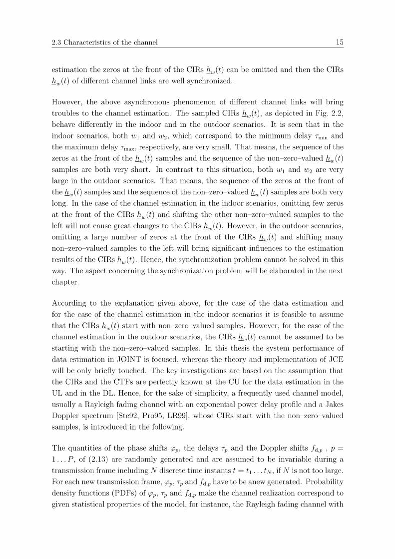
However, the above asynchronous phenomenon of different channel links will bring
troubles to the channel estimation. The sampled CIRs hw(t), as depicted in Fig. 2.2,
behave differently in the indoor and in the outdoor scenarios. It is seen that in the
indoor scenarios, both w1 and w2, which correspond to the minimum delay τmin and
the maximum delay τmax, respectively, are very small. That means, the sequence of the
zeros at the front of the hw(t) samples and the sequence of the non–zero–valued hw(t)
samples are both very short. In contrast to this situation, both w1 and w2 are very
large in the outdoor scenarios. That means, the sequence of the zeros at the front of
the hw(t) samples and the sequence of the non–zero–valued hw(t) samples are both very
long. In the case of the channel estimation in the indoor scenarios, omitting few zeros
at the front of the CIRs hw(t) and shifting the other non–zero–valued samples to the
left will not cause great changes to the CIRs hw(t). However, in the outdoor scenarios,
omitting a large number of zeros at the front of the CIRs hw(t) and shifting many
non–zero–valued samples to the left will bring significant influences to the estimation
results of the CIRs hw(t). Hence, the synchronization problem cannot be solved in this
way. The aspect concerning the synchronization problem will be elaborated in the next
chapter.
According to the explanation given above, for the case of the data estimation and
for the case of the channel estimation in the indoor scenarios it is feasible to assume
that the CIRs hw(t) start with non–zero–valued samples. However, for the case of the
channel estimation in the outdoor scenarios, the CIRs hw(t) cannot be assumed to be
starting with the non–zero–valued samples. In this thesis the system performance of
data estimation in JOINT is focused, whereas the theory and implementation of JCE
will be only briefly touched. The key investigations are based on the assumption that
the CIRs and the CTFs are perfectly known at the CU for the data estimation in the
UL and in the DL. Hence, for the sake of simplicity, a frequently used channel model,
usually a Rayleigh fading channel with an exponential power delay profile and a Jakes
Doppler spectrum [Ste92, Pro95, LR99], whose CIRs start with the non–zero–valued
samples, is introduced in the following.
The quantities of the phase shifts ϕp, the delays τp and the Doppler shifts fd,p , p =
1 . . . P , of (2.13) are randomly generated and are assumed to be invariable during a
transmission frame including N discrete time instants t = t1 . . . tN , if N is not too large.
For each new transmission frame, ϕp, τp and fd,p have to be anew generated. Probability
density functions (PDFs) of ϕp, τp and fd,p make the channel realization correspond to
given statistical properties of the model, for instance, the Rayleigh fading channel with

16 Chapter 2: Channel models
an exponential power delay profile and a Jakes Doppler spectrum [Ste92, Pro95, LR99].
Generally, the phase shifts ϕp are independent realizations of the random variable ϕ
with a uniform distribution in [0,2π), i.e., the PDF of ϕ in [Ste92]
pϕ(ϕ) =
{12π
for ϕ ∈ [0, 2π),0 else.
(2.14)
For the widely–used exponentially decreasing power delay profile [COS89], if a denotes
the exponent of the power delay profile and can be determined by
a =3 ln 10
τmax
, (2.15)
the delays τp are independent realizations of a random variable τ with the PDF [Ste92]
pτ (τ) =
{ a1−exp(−aτmax)
exp (−aτ) for 0 ≤ τ < τmax,
0 else.(2.16)
If the multipath signals are received from all directions with equal probabilities, with
fd,max denoting the maximum Doppler shift, the Doppler shifts fd,p are independent
realizations of a random variable fd with a Jakes PDF [Ste92, Pro95, LR99]
pfd(fd) =
1
πfd,max
√1−
(fd
fd,max
)2for |fd| ≤ fd,max,
0 else.
(2.17)
Following (2.14), (2.16) and (2.17), the phase shifts ϕp, the excess delays τp and the
Doppler shifts fd,p are generated so that the CIR vector h(t) and CTF vector h(t) can
be realized to describe the Rayleigh fading channel with an exponential power delay
profile and a Jakes Doppler spectrum [Ste92, Pro95, LR99], which is to be applied in
the data estimation for the scenarios in which the transmitter or the receivers make
small–scale movement in this thesis.
2.3.2 Slow fading
Due to the shadowing effect during the propagation, the power received fluctuates
with time slowly as the transmitter or the receiver moves in a large scale [Par92, LR99,
Pro95]. This phenomenon is termed slow fading or large–scale fading. Generally the
log–normal fading is suitable for modelling shadowing effects caused by obstacles during
the propagation [Par92, Pro95, LR99]. Therefore, slow fading can be also termed log–
normal fading.

2.3 Characteristics of the channel 17
��
��
�
Fig. 2.3. Two–ray model
For the power Pt(t) transmitted at the time instant t, the power Pr(t) received is given
by [Par92, Pro95, LR99]
Pr(t) = g(t) · Pt(t), (2.18)
where g(t) is the linear path gain of the corresponding propagation channel. The linear
path gain g(t) obeys approximately a log–normal distribution [Par92, Pro95, LR99],
i.e., the logarithm
G(t) = 10 log10 g(t) (2.19)
can be approximated as a Gaussian variable with a standard deviation σG and a mean
value G.
In reality the standard deviation σG usually takes values between 0 . . . 10 dB according
to the environment [COS91, Par92, BARY96, DB96, LR99].
The average logarithmic path gain G, which depends on the distance ρ between the
transmitter and the receiver, has to be determined according to the considered scenario.
There are many outdoor path loss models [COS91, Par92, BARY96, DB96, LR99] to
describe the average logarithmic path gain G, on the basis of either theoretical analysis
or on measurement results in different propagation scenarios. Some of these models
are introduced briefly in the following:
• The free space model [Par92]: The average logarithmic path gain G decreases in
the free space at a decay rate of 20 dB/decade [Par92, LR99], i.e., G drops 20
dB as ρ gets ten times larger.
• The two–ray model depicted in Fig. 2.1: Since one reflected path is taken into
account [Par92] beyond one direct path from the transmitter to the receiver, the
average logarithmic path gain G drops at a decay rate of about 40 dB/decade
[Par92].

18 Chapter 2: Channel models
100
101
102
103
104
−160
−140
−120
−100
−80
−60
−40
���
�����
Fig. 2.4. An example of the dual–slope model, when, e.g., gT =gR = 1, α1 = 2.0, α2 = 4.0 and ρB = 300m hold
• The COST–231–Hata model and COST–231–Walfish–Ikegami model [COS91]:
These two models are the results of experiments performed under the conditions
described in [COS91].
All the models mentioned above have one point in common: The average logarithmic
path gain G drops versus the distance ρ with a constant decay rate. However, more
and more measurement results [HN80, Ste92, XBMLS92] indicate that in most outdoor
environments the decay rate of the average logarithmic path gain G versus the distance
ρ is not a constant value, in other words, this decay rate depends on the distance ρ
[XBMLS92]. In order to model the channel more accurately, a dual–slope model is pro-
posed with the concept of the break–even–point distance ρB [XBMLS92]. With α1 and
α2 denoting the two different attenuation exponents, respectively, which describe the
two different decay rates, and with λ denoting the wavelength, the average logarithmic
path gain G versus the distance ρ is given by
G/dB =
{ −10α1 log10
(4πρλ
)+ 10 log10 (gTgR) for 0 ≤ ρ < ρB,
−10α1 log10
(4πρB
λ
)+ 10 log10 (gTgR)− 10α2 log10
(ρ
ρB
)for ρ ≥ ρB,
(2.20)
where gT and gR denote the antenna gains of the transmit antenna and the receive
antenna, respectively [XBMLS92]. According to (2.20) the average logarithmic path
gain G decreases with the decay rate equal to 10α1 dB/decade within the break–even–
point range, that is for ρ < ρB, and with the decay rate equal to 10α2 dB/decade out

2.3 Characteristics of the channel 19
of the break–even–point range, that is for ρ ≥ ρB, where α1 < α2 holds, as depicted in
Fig. 2.4. The values of the attenuation exponents α1, α2 and of the break–even–point
distance ρB should be chosen according to the indicated scenario.
For the resultant of two independent stochastic processes, fast fading and slow fading,
the modified CIR vector h′(t) can be obtained by multiplying the CIR vector h(t) of
(2.1) with a factor√
g(t), that is
h′(t) =√
g(t) · h(t). (2.21)
Consequently, the modified CTF vector h′(t) can be obtained by multiplying the CTF
vector h(t) of (2.3) also with the factor√
g(t)
h′(t) =
√g(t) · h(t). (2.22)
This modified channel model including the Rayleigh fading mentioned in Subsection
2.3.1 and the log–normal fading described in this subsection is applied in the data
estimation for the outdoor urban scenarios considered in this thesis.

20
Chapter 3
JOINT: A multipoint–to–multipointOFDM system
3.1 Motivation
In order to generate a solid basis for the considerations in the following chapters,
in the present Chapter 3 an expansion from the conventional point–to–point OFDM
transmission [Doe57, WE71, PR80, Bin90, Pra98, KS01, FK03] to the multipoint–to–
multipoint OFDM transmission, which is applied in JOINT, is first discussed in Section
3.2. The problem of time synchronization in JOINT is basically addressed in Section
3.3. Finally the parameter values to be applied in the numerical simulations of JOINT
are given in Section 3.4. In what follows, the consideration is with respect to the time
instant t. Therefore, for the sake of simplicity, t will be omitted in the notation if it is
not declared otherwise.
3.2 OFDM transmission technique
OFDM is a multiplexing and modulation technique gaining considerable interest in
recent years. Moreover, OFDM is applied in numerous communications systems over
the world [ETS97b, ETS97c, RCLF89, RS95, TL97, Cim85, Bin91, CTC91, Jon95,
IEE99, CWKS97, vNAM+99, ETS96, ETS99]. The advantages and disadvantages of
the OFDM transmission technique have been elaborated in lots of publications, e. g.
[Bin90, Pra98, vNP00, KS01]. In the following the application of OFDM in JOINT is
addressed.
Generally, a mobile radio system can be described by a linear transmission structure
(LTS) as the one illustrated in Fig. 3.1.a. The mobile radio channels considered in
this thesis are assumed to be linear. Here, the LTS consists of the modulator in the
transmitter, the linearly modelled mobile radio channel and the demodulator at the
receiver. At the input of the LTS, the vector
x =(x(1) . . . x(N)
)T(3.1)
containing N complex values of the input signal is fed into the LTS. At the receiver,
i. e., the output of the LTS, the vector
y =(y(1) . . . y(M)
)T(3.2)
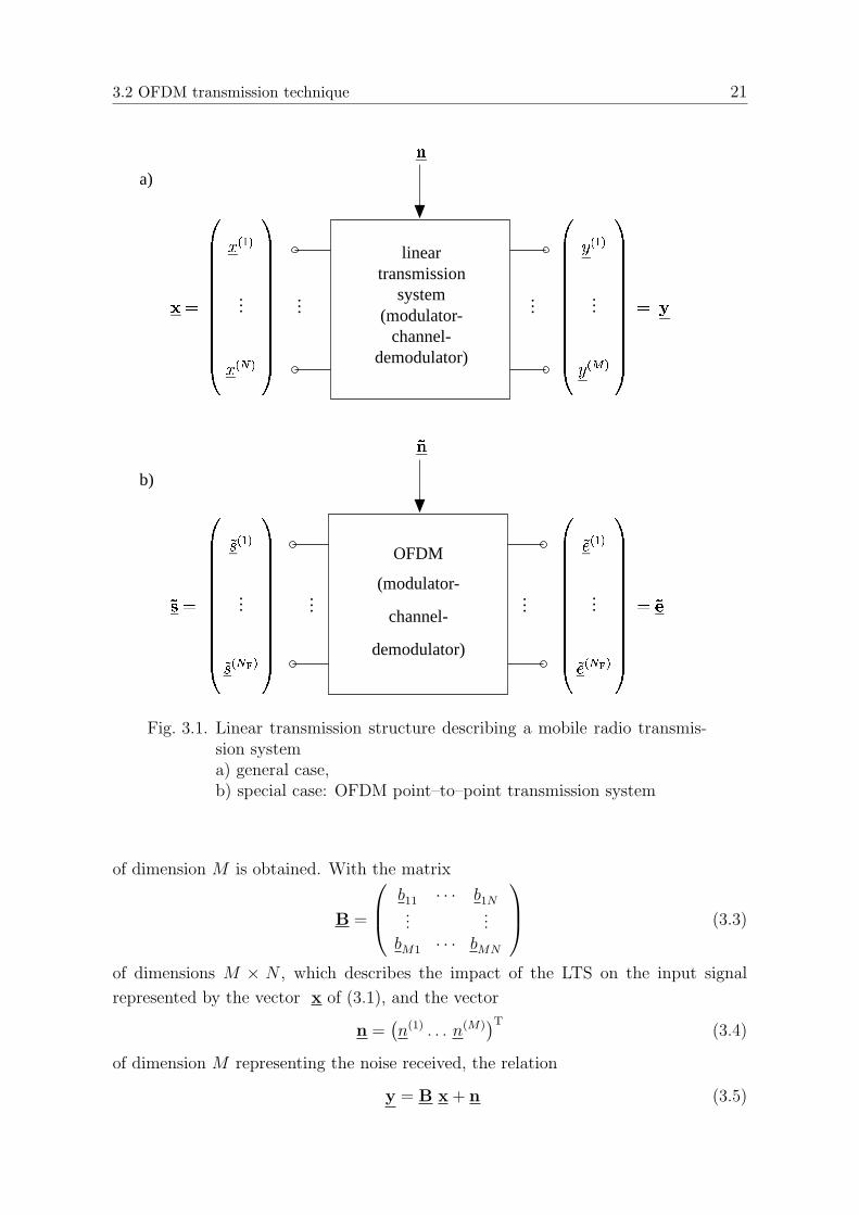
3.2 OFDM transmission technique 21
��
(modulator-
channel-
demodulator)
lineartransmission
system(modulator-
channel-demodulator)
b)
�������������
�������������
�������������
�������������
���
� ��
...
����
�� ��
... ������ ......
a)
�������������
�������������
�������������
�������������
���
���
...
���
� �
... ���� ......
�
OFDM
Fig. 3.1. Linear transmission structure describing a mobile radio transmis-sion systema) general case,b) special case: OFDM point–to–point transmission system
of dimension M is obtained. With the matrix
B =
b11 · · · b1N...
...bM1 · · · bMN
(3.3)
of dimensions M × N , which describes the impact of the LTS on the input signal
represented by the vector x of (3.1), and the vector
n =(n(1) . . . n(M)
)T(3.4)
of dimension M representing the noise received, the relation
y = B x + n (3.5)

22 Chapter 3: JOINT: A multipoint–to–multipoint OFDM system
holds between the input vector x of (3.1) and the output vector y of (3.2) of the LTS.
As it can be observed from the structure of the matrix B of (3.3), in general relations
exist between each of the elements of x on the one side and y on the other side, which
constitute a challenge for the equalization at the receiver of the LTS.
One special case of a LTS is illustrated in Fig. 3.1.b, where a point–to–point OFDM
transmission system is presented in the frequency domain. In the case of OFDM, both
the input vector
s =(s1 . . . sNF
)T(3.6)
and the output vector
e =(e1 . . . eNF
)T(3.7)
consist of NF complex amplitudes, where NF denotes the number of subcarriers. With
the noise vector
n =(n1 . . . nNF
)T, (3.8)
(3.5) is rewritten as
e = B s + n . (3.9)
The speciality of OFDM lies in the structure of the matrix B of (3.3) and (3.9). It can be
seen from (3.6), (3.7) and (3.9) that for the typical OFDM point–to–point transmission
the matrix B is square. Further, in the OFDM applying LTS of Fig. 3.1.b, the structure
modulator – channel – demodulator is represented by the structure inverse fast Fourier
transform (IFFT) – cyclic prefix addition – channel – cyclic prefix removal – FFT
[WE71, Bin90, Pra98]. Due to this special LTS structure in the case of OFDM,
bmn =
{bnF
for n = m, nF = 1 . . . NF,0 else
(3.10)
holds for the elements of B, i.e., B is a diagonal matrix. Therefore, the equalization
task at the receiver of the LTS [Bin90, Pra98, FK03] can be facilitated. Due to the fact
that the matrix B of (3.3) becomes diagonal for the OFDM applying LTS of Fig. 3.1.b,
the relation between the vector s of the transmitted signal of (3.6) and the vector e
of the receive signal of (3.7) can be examined subcarrierwise.
Extending these considerations to JOINT, the structure depicted in Fig. 3.1.b repre-
sents the link between an arbitrary pair of an MT and an AP in the considered SA.
Therefore, JOINT is a multipoint–to–multipoint OFDM system. For instance, in the
UL of JOINT it is assumed that in the SA there are KB APs distributed and K MTs
simultaneously active, each being equipped with a single antenna. In this case, the
matrix B in (3.9), is represented by the channel matrix
H(k, kB)
=
h(k,kB)
1 · · · 0...
. . ....
0 · · · h(k,kB)
NF
∈ CNF×NF , (3.11)

3.2 OFDM transmission technique 23
between the MT k, k = 1 . . . K, and the AP kB, kB = 1 . . . KB, where the values h(k,kB)
nF,
nF = 1 . . . NF, denote the CTFs of the subcarriers between the MT k and the AP kB.
With (3.11), (3.5) is rewritten as
e(kB)u = H
(k, kB)s(k)u + n(kB)
u . (3.12)
For such a multiple–MT and multiple–AP scenario the total channel matrix contains
several diagonal submatrices describing the mobile radio channels between each MT k,
k = 1 . . . K, and each AP kB, kB = 1 . . . KB, i.e.,
Hu =
H(1,1) · · · H
(K,1)
......
H(1,KB) · · · H
(K,KB)
(3.13)
holds. With (3.13), with the total vector
su =(
s(1)u
T. . . s(K)
u
T)T
(3.14)
of the transmitted signals of dimension KNF, with the total vector
eu =(e(1)
u
T. . . e(KB)
u
T)T
(3.15)
of the receive signals of dimension KBNF and with the total vector
nu =(
n(1)u
T. . . n(KB)
u
T)T
(3.16)
of the noise vector of dimension KBNF, (3.12) takes the form
eu = Hu su + nu (3.17)
for the multiple–MT and multiple–AP scenario in the UL of JOINT. With the appli-
cation of the simple OFDM transmitter at the MTs su is either the transmitted data
vector
du =(d
(1)
u,1 . . . d(1)
u,NF. . . d
(K)
u,1 . . . d(K)
u,NF
)T
(3.18)
of dimension KNF for the data transmission or the pilot vector
p =(p(1)
1. . . p(1)
NF. . . p(K)
1. . . p(K)
NF
)T
(3.19)
of dimension KNF for JCE.
With (3.11), (3.13) and (3.17) it becomes obvious that due to the application of OFDM,
the subcarrierwise investigation is feasible in the multiple–MT and multiple–AP case
of JOINT and results in a relaxed computational effort in data estimation at the CU.

24 Chapter 3: JOINT: A multipoint–to–multipoint OFDM system
Therefore, a subcarrierwise representation is favorable, if data estimation is considered,
i.e.,
e(1)u,nF...
e(KB)u,nF
︸ ︷︷ ︸eu,nF
=
h(1,1)
nF· · · h
(K,1)
nF...
...
h(1,KB)
nF· · · h
(K,KB)
nF
︸ ︷︷ ︸Hu,nF
·
s(1)u,nF...
s(K)u,nF
︸ ︷︷ ︸su,nF
+
n(1)u,nF...
n(KB)u,nF
︸ ︷︷ ︸nu,nF
(3.20)
holds for the corresponding subcarrier nF, nF = 1 . . . NF.
In the DL, with (3.11) (3.5) can be rewritten as
e(k)d = H
(k, kB)s(kB)d + n
(k)d (3.21)
for the DL transmission. Due to the reciprocity of the UL and the DL channel in the
application of TDD, the total channel matrix in the DL
Hd = Hu
T=
H(1,1) · · · H
(1,KB)
......
H(K,1) · · · H
(K,KB)
(3.22)
holds. With (3.22), with the total vector
sd =(
s(1)d
T. . . s
(KB)d
T)T
(3.23)
of the transmitted signals of dimension KBNF, with the total vector
ed =(e
(1)d
T. . . e
(K)d
T)T
(3.24)
of the receive signals of dimension KNF and with the total vector
nd =(
n(1)d
T. . . n
(K)d
T)T
(3.25)
of the noise vector of dimension KNF, (3.21) takes the form
ed = Hd sd + nd (3.26)
for the multiple–MT and multiple–AP scenario in the DL of JOINT, where sd is the
designed on the basis of the transmitted data vector
dd =(d
(1)
d,1 . . . d(1)
d,NF. . . d
(K)
d,1 . . . d(K)
d,NF
)T
(3.27)
of dimension KNF.

3.3 Time synchronization 25
� � � �� � � �� � � �� � � �
� � � � � � � � � � � � �� � � � � � � � � � � � �� � � � � � � � � � � � �� � � � � � � � � � � � �
� � � � � � � � � � � � �� � � � � � � � � � � � �� � � � � � � � � � � � �� � � � � � � � � � � � �� � � �� � � �� � � �� � � �
Ts
Toss
Tcp
Fig. 3.2. Temporal structure of an OFDM slot
Moreover, the subcarrierwise DL transmission of JOINT reads
e(1)d,nF...
e(K)d,nF
︸ ︷︷ ︸ed,nF
=
h(1,1)
nF· · · h
(1,KB)
nF...
...
h(K,1)
nF· · · h
(K,KB)
nF
︸ ︷︷ ︸Hd,nF
=HT
u,nF
·
s(1)d,nF...
s(KB)d,nF
︸ ︷︷ ︸sd,nF
+
n(1)d,nF...
n(K)d,nF
︸ ︷︷ ︸nd,nF
. (3.28)
3.3 Time synchronization
A crucial task in OFDM systems are time and frequency synchronization [KMH98,
vNP00, FK03]. In this section we consider the time synchronization problem. As
the point–to–point OFDM system is extended to the multipoint–to–multipoint OFDM
system a new problem of time synchronization arises, which will be explained and
solved in the following. Before we go deeper into the topic, it is necessary to briefly
introduce some basics, e.g., on the OFDM symbol structure.
Each OFDM symbol slot consists of two parts [Pra98, vNP00, FK03]:
• The OFDM symbol of duration Ts, which contains the data or the pilots to be
transmitted by being mapped on the subcarriers, and
• the above mentioned cyclic prefix of duration Tcp, which contains a cyclic exten-
sion of the OFDM symbol [PR80, vNP00].
Consequently,
Toss = Ts + Tcp (3.29)
holds for the duration of the OFDM symbol slot, as depicted in Fig.3.2.

26 Chapter 3: JOINT: A multipoint–to–multipoint OFDM system
�������
AP AP 2
MT 2
MT 1
AP 1
MT 1
MT 2
a) b)
���������
���������
���������
���������
�������
Fig. 3.3. Time synchronization issues in the ULa) multipoint–to–point transmissionb) multipoint–to–multipoint transmission as in JOINT
In the case of point–to–point OFDM transmission systems time synchronization is a
well studied problem which can be solved by controlling the timing reference of e.g.,
the transmitter [vNP00, FK03].
If we extend such a point–to–point system to a multipoint–to–point system as shown
in Fig. 3.3a with different time delays between the MTs and the APs, there are also
well known solutions to the time synchronization problem [KMH98, vdBBB+99]. To-
tally different is the situation in the case of JOINT, see Fig. 3.3b, where we have a
multipoint–to–multipoint system. In such a system, in the example of Fig. 3.3b we
consider the case K equal to two, it is generally impossible to achieve that the signals
of MT 1 and MT 2 arrive synchronously both at AP 1 and AP 2. An exception would
be the particular situation that all distances between APs and MTs would be equal. In
what follows we will briefly show how time synchronization of JOINT can be achieved
in situations as the one shown in Fig.3.3b.
Fig. 3.4 shows schematically the magnitudes of the four CIRs h(k, kB)(τ), k, kB ∈ {1, 2}introduced in Fig. 3.3b. In this example the smallest possible value of Tcp would be
given by
Tcp,min = τ (1,1)max − τ
(1,2)min = τsup − τ
(1,2)min . (3.30)
τsup denotes the supremum of the maximum delays. Therefore with respect to the time
synchronization problem in JOINT we propose to choose
Tcp ≥ τsup. (3.31)
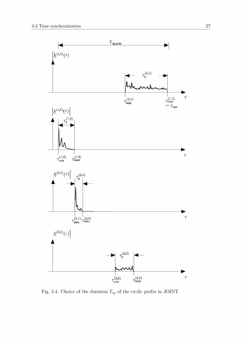
3.3 Time synchronization 27
0 10 20 30 40 50 60 701
1.1
1.2
1.3
1.4
1.5
1.6
1.7
1.8
1.9
0 700.5
1
1.5
2
10 20 30 40 50 60 700
0.05
0.1
0.15
0.2
0.25
0 700.5
1
1.5
2
�����������
���
�
�
�
�
�����������
���
�����������
���
�����������
���
��� ��
�����
������ ���
����� ��
�������
������ ���
����� ��
������ ���
����� ��
�������
�������
�������
������ ��
������ ��
Fig. 3.4. Choice of the duration Tcp of the cyclic prefix in JOINT

28 Chapter 3: JOINT: A multipoint–to–multipoint OFDM system
OFDM symbol slots
subc
arri
ers
time
11
freq
uenc
y
Tfr = NB · Toss
B=
NF
·∆
fn
F
NB
Toss
NF
Fig. 3.5. Time–frequency representation of an OFDM frame
3.4 Parametrization of JOINT
The design of an OFDM based system like JOINT demands a trade–off between various
system requirements and channel properties, which, into the bargain, often conflict with
each other. This section presents important parameters and relations between them in
order to achieve a proper design of JOINT.
Fig. 3.5 illustrates the time–frequency representation of an OFDM frame as applied
in JOINT. In the time direction, one OFDM frame stretches out over a total of NB
OFDM symbol slots. Each OFDM symbol slot nB, nB = 1 . . . NB, covers the NF
available subcarriers in the frequency direction. Adjacent subcarriers are spaced by
∆fnFapart. The duration Tfr of an OFDM frame is given by the product of the
number NB of OFDM symbol slots and the duration Toss of one OFDM symbol slot,
i. e.,
Tfr = NB · Toss, (3.32)
whereas the product of the number NF of available subcarriers and the subcarrier

3.4 Parametrization of JOINT 29
spacing ∆fnFgives the system bandwidth B, i. e.,
B = NF ·∆fnF. (3.33)
Now, following the well known rationale of OFDM [WE71, Bin90, vNP00, FK03],
certain relations have to be fulfilled between the quantities of, such as, the subcarrier
spacing ∆fnF, the OFDN symbol duration Ts, the supremum τsup of the maximum
delays and the cyclic prefix duration Tcp.
In order to achieve the orthogonality between the adjacent subcarriers typical for
OFDM [Bin90, vNP00, FK03],
Ts ·∆fnF= 1 (3.34)
has to be valid. The cyclic prefix duration Tcp must be chosen in such a way that
it at least exceeds the supremum of the maximum delay τsup of the CIR, which is
approximately the reverse of the coherence bandwidth Bc of the channel, to overcome
the frequency selectivity, i.e.,
Tcp ≥ 1
Bc
≈ τsup (3.35)
is to be met. Providing a cyclic prefix of the required non–zero duration Tcp reduces
transmission capacity and is the price to be paid for enabling low cost signal processing
at the receiver by FFT also in the case of radio channels exhibiting a non–zero delay
spread [PR80, Bin90, Pra98, vNP00, FK03]. This price can be quantified by a quantity
Tcp/Ts termed overhead. Usually, in OFDM systems
Tcp/Ts = 0.1 . . . 0.25 (3.36)
holds for the overhead [PR80, Bin90, Pra98, vNP00, FK03] so that the overhead Tcp/Ts
introduced by the insertion of the cyclic prefix is kept as low as possible. According to
(3.33), (3.34) and (3.36) the subcarrier spacing ∆fnFis given by
∆fnF=
B
NF
=1
Ts
=1
4 . . . 10 Tcp
. (3.37)
With (3.35) and (3.37) follows
Bc ≈ 1
τsup
≈ 1
Tcp
= 4 . . . 10 ∆fnF. (3.38)
One of the drawbacks of the OFDM transmission technique is its sensitivity to Doppler
shifts [vNP00, KS01, FK03]. A measure for the Doppler shift is the maximum Doppler
frequency fd,max. With the carrier frequency fc, the maximum relative velocity vmax
between transmitter and receiver and the speed c0 of light
fd,max = fcvmax
c0
, (3.39)

30 Chapter 3: JOINT: A multipoint–to–multipoint OFDM system
Table 3.1. System parametrization of JOINT
Parameter Value
supremum of maximum delays τsup = 5 µscoherence bandwidth Bc=200 kHz
carrier frequency fc=5.5 GHzmaximum speed vmax=200 km/h
maximum Doppler frequency fd,max=1.018 kHzbreak–even–point distance ρB = 300 m
attenuation exponents α1 = 2.0 and α2 = 4.0antenna gains gT = gR = 1
system bandwidth B=20 MHzOFDM symbol duration Ts = 25.6 µscyclic prefix duration Tcp = 6.4 µs
OFDM symbol slot duration Toss = 32 µsnumber of subcarriers (FFT length) NF=512
subcarrier spacing ∆fnF=39.063 kHz
modulation QAM
holds [Kam96, Hay01]. The sensitivity of OFDM to Doppler shifts is negligible if
∆fnFÀ fd,max (3.40)
holds as a requirement to be observed in OFDM system design.
To describe the log–normal fading the break–even–point distance ρB of (2.20) is as-
sumed to be 300 m for the typical outdoor environment. The two attenuation exponents
α1 and α2 of (2.20) are assumed to be equal to 2.0 and 4.0, respectively. Moreover,
the antenna gains gT and gR of the transmit antenna and the receive antenna are both
assumed to be one.
In order to illustrate the theoretical considerations of this thesis by quantitative exam-
ples, a certain parameter set of JOINT should be chosen. Table 3.1 gives the chosen
system parametrization of JOINT.
31
Chapter 4
Maximum–likelihood joint channelestimation in the uplink of JOINT
4.1 Preliminary remarks
An important presupposition of the data detection and transmission of JOINT is that
channel state information (CSI) is known at the CU. The task to estimate the CIRs
and the CTFs is performed by JCE at the CU in the UL of JOINT. JCE, a pilot–aided
multiuser channel estimation technique [SMWB01, MWSL02], aims at estimating all
the CTFs between MTs and APs in a SA simultaneously with the aid of the pilot
signals in the UL, which have special properties known both at the transmitters and
receivers. In JOINT it is assumed that the pilot symbols are transmitted once in the
middle of an OFDM frame, which contains a number of symbol slots assigned to the
UL and the DL symbols.
4.2 System model
The pilot symbols radiated by MT k, k = 1 . . . K, can be either stacked in an MT–
specific pilot vector
p(k) =(p(k)
1. . . p(k)
NF
)T
(4.1)
of dimension NF, which forms a part of the total pilot vector of (3.19), or in an NF×NF
diagonal pilot matrix [SMWB01, MWSL02]
P(k)
=
p(k)
1· · · 0
.... . .
...
0 · · · p(k)
NF
. (4.2)
With P(k)
of (4.2) the total pilot matrix
P =(
P(1)
. . . P(K)
)(4.3)
of dimensions NF × (KNF) can be established [SMWB01, MWSL02]. According to
(2.1) and (2.3), the K unknown CIR vectors
h(k,kB) =(h
(k,kB)1 . . . h
(k,kB)W
)T
(4.4)

32 Chapter 4: Maximum–likelihood joint channel estimation in the uplink of JOINT
valid for AP kB, kB = 1 . . . KB, can be stacked in an AP–specific CIR vector
h(kB) =(h(1,kB)T . . . h(K,kB)T
)T
(4.5)
of dimension KW , and the K unknown CTF vectors
h(k,kB)
=(h
(k,kB)
1 . . . h(k,kB)
NF
)T
(4.6)
valid for the AP kB can be stacked in an AP–specific CTF vector
h(kB)
=
(h
(1,kB)T
. . . h(K,kB)T
)T
(4.7)
of dimension KNF. It is assumed that at the AP kB the AP–specific receive vector
e(kB)h =
(e(kB)h,1 . . . e
(kB)h,NF
)T
(4.8)
of dimension NF is corrupted by the noise vector
n(kB)h =
(n
(kB)h,1 . . . n
(kB)h,NF
)T
(4.9)
of dimension NF. With (4.3), (4.7) and (4.9)
e(kB)h = P h
(kB)+ n
(kB)h (4.10)
holds for the AP–specific receive vector of (4.8) [SMWB01, MWSL02], where the K NF
unknown elements of the AP–specific CTF vector h(kB)
of (4.7) have to be determined.
During the time slot for the pilot transmission in the UL, the pilot energies
E(k)p,nF
=1
2|p(k)
nF|2 = Ep, k = 1 . . . K, nF = 1 . . . NF, (4.11)
invested for the pilot symbols p(k)
nFof (4.1) are assumed to be equal. If n
(kB)h of (4.9) is
uncorrelated,
E{
n(kB)h n
(kB)h
∗T}= 2σ2INF , kB = 1 . . . KB, (4.12)
follows for the covariance matrix of n(kB)h with σ2 denoting the variance of the real and
the imaginary parts of the components of n(kB)h . In the SA full system load is assumed
to hold in the following, that is
NF = K ·W. (4.13)

4.3 Algorithm of joint channel estimation 33
4.3 Algorithm of joint channel estimation
The goal of JCE is to obtain the CTF estimates on the basis of the information of the
AP–specific receive vector e(kB)h , kB = 1 . . . KB, of (4.10) and the total pilot matrix P
of (4.3).
With a (KNF)× (KW ) block–diagonal matrix [SMWB01, MWSL02]
FW,tot =
[F ]1,1NF,W · · · 0...
. . ....
0 · · · [F ]1,1NF,W
, (4.14)
whose diagonal submatrices are the dimension–reduced Fourier matrices [F ]1,1NF,W of
(2.9), and with the AP–specific CIR vector h(kB) of (4.5), (2.9) is rewritten as
h(kB)
= FW,toth(kB) (4.15)
for the multiple–MT and multiple–AP scenario with respect to the AP kB. With (4.15)
(4.10) can be rewritten as [SMWB01, MWSL02]
e(kB)h = P FW,tot︸ ︷︷ ︸
G
h(kB) + n(kB)h . (4.16)
In order to minimize the mean square error E{||e(kB)
h − G h(kB)||2
}the estimate
h(kB)
=(G∗TG
)−1
G∗Te
(kB)h (4.17)
of the AP–specific CIR vector h(kB) of (4.5) can be obtained [SMWB01, MWSL02]. If
the white noise n(kB)h of (4.9) also yields to Gaussian distribution, the estimate h
(kB)of
(4.17) is the maximum–likelihood (ML) estimate. Obviously, FW,tot is known once NF
and W are chosen. The number of the unknowns concerning the AP–specific channels
is reduced from KNF to KW . With (4.15) and (4.17) the unbiased estimate of the
AP–specific CTF vector h(kB)
is given by [SMWB01, MWSL02]
ˆh(kB)
= FW,tot
(G∗TG
)−1
G∗T
︸ ︷︷ ︸Z
e(kB)h
= h(kB)
+ Z n(kB)h . (4.18)
(4.16) and (4.18) show that either the matrix G or the matrix Z contains the matrix
FW,tot, i.e., the receive signals on all the subcarriers have to be processed jointly.

34 Chapter 4: Maximum–likelihood joint channel estimation in the uplink of JOINT
Therefore, JCE is not a subcarrierwise process. Once the pilot matrix P is chosen for
the transmission, the matrices G and Z are fixed, since the matrix FW,tot is constant
for the given K, W and NF. Moreover, for all the APs the matrices G and Z are the
same because the design of the pilot matrix P is regardless of the APs. These facts
can be utilized in the implementation of the algorithm.
4.4 Choice of the pilot vectors
As stated previously, the pilot vectors are not only known both at the MTs and the CU,
but also have some special properties so that the estimates ˆh(kB)
of the h(kB)
of (4.18)
with good performances can be obtained without too much effort. Now a question
arises: Which kind of vectors can be chosen as the pilot vectors p(k) of (4.1)?
To answer the above question, the performance evaluation criterion of JCE is first dis-
cussed. In [SMWB01, MWSL02] the signal–to–noise–ratio (SNR) degradation is intro-
duced as an evaluation criterion for JCE in the presence of the noise. The SNR degrada-
tion is defined as the ratio of the SNR obtained in a reference case and the SNR obtained
by JCE. The single MT case is chosen as the reference case [SMWB01, MWSL02], where
the MT k uses all the NF available subcarriers for the pilot transmission, e.g., the pilot
vector
p(k)
ref=
√2Ep
1 . . . 1︸ ︷︷ ︸
NF
T
(4.19)
for the considered MT k is transmitted. Then the reference SNR
γ(k,kB)ref,nF
=EpNF
2σ2W
∣∣∣h(k,kB)
nF
∣∣∣2
(4.20)
for the estimate ˆh(k,kB)
nFof the CTF h
(k,kB)
nFat the output of the joint channel estimator
is obtained [SMWB01, MWSL02]. With (4.18) follows the SNR
γ(k,kB)nF
=
∣∣∣h(k,kB)
nF
∣∣∣2
∣∣∣∣h(k,kB)
nF− ˆh
(k,kB)
nF
∣∣∣∣2
=
∣∣∣h(k,kB)
nF
∣∣∣2
2σ2[
Z Z∗T]
i,i
, i = (k − 1)NF + nF, (4.21)

4.4 Choice of the pilot vectors 35
of the estimate ˆh(k,kB)
nFof the CTF h
(k,kB)
nF[SMWB01, MWSL02]. Consequently, with
(4.20) and (4.21) the SNR degradation
δ(k,kB)nF
=γ
(k,kB)ref,nF
γ(k,kB)nF
=EpNF
W[ Z Z
∗T]i,i, i = (k − 1)NF + nF, (4.22)
can be obtained [SMWB01, MWSL02]. In (4.22) the diagonal elements of Z Z∗T
are
anti–proportional to the pilot energy Ep so that the SNR degradations δ(k,kB)nF do not
depend on the pilot energy Ep [SMWB01, MWSL02]. With (4.16), (4.18) and (4.22)
it is seen that for a given scenario where the parameters Ep, W , K and NF are chosen,
the matrix product Z Z∗T
and the SNR degradations δ(k,kB)nF of (4.22) depend only on
the chosen pilot vectors p(k) of (4.1)[SMWB01, MWSL02].
The goal to design the pilot vectors p(k) of (4.1) for JCE is to obtain the SNR degrada-
tions δ(k,kB)nF of (4.22) as small as possible [SMWB01, MWSL02]. A good example of the
pilot vectors is designed on the basis of the well known Walsh codes [Pro95, MWSL02],
whose SNR degradations δ(k,kB)nF at the output of the joint channel estimator are equal
to 1. In the frequency domain, the Walsh codes to be assigned to the MTs as pilots are
chosen from the columns of the NF ×NF Hadamard matrix [Pro95]. E.g., for NF = 8
follows the 8× 8 Hadamard matrix
W8 =
1 1 1 1 1 1 1 11 −1 1 −1 1 −1 1 −11 1 −1 −1 1 1 −1 −11 −1 −1 1 1 −1 −1 11 1 1 1 −1 −1 −1 −11 −1 1 −1 −1 1 −1 11 1 −1 −1 −1 −1 1 11 −1 −1 1 −1 1 1 −1
. (4.23)
According to (4.23) it is seen that if the pilots based on the Walsh codes are applied
for JCE, all the NF subcarriers are utilized simultaneously for the MTs and there may
exist many different sets of pilots, since K ≤ NF is always valid in JOINT.
In this thesis, the pilot vectors based on the Walsh codes are applied for JCE.
36
Chapter 5
Linear zero–forcing joint detection in theuplink of JOINT
5.1 Preliminary remarks
As mentioned in Chapter 1 the CU minimizes the intra–SA MAI among the various
simultaneously active links in the considered SA in the UL through JD, which belongs
to the category of multiuser detection (MUD) [Ver98]. There are some optimum MUD
approaches, e.g., the maximum a posteriori (MAP) sequence estimation [Ver86] and
the maximum–likelihood (ML) sequence estimation [For72, Ver98] algorithms. How-
ever, such search processes for the data estimates are too computation–consuming and
limit their application. Some suboptimum linear JD algorithms [Kle96, Ver98, Bla98]
exist, which form a compromise between the system performance and the computa-
tional complexity, e.g., the zero–forcing (ZF) [Kle96, Ver98, Bla98, Skl04] JD and the
minimum–mean–square–error (MMSE) [Kle96, Skl04] JD. In JOINT, the applied JD
algorithm can be chosen from various options. For the sake of simplicity the linear
receive–ZF (RxZF) JD is focused on in this thesis.
A subcarrierwise investigation of the data detection in the uplink is feasible due to the
application of OFDM according to Chapter 3. Therefore, in the following sections the
subcarierwise representations are used.
5.2 System model in the uplink of JOINT
For the OFDM based UL of JOINT, the subcarrierwise data transmission is illustrated
in Fig.5.1. In a SA, KB APs are fixedly located and connected to the CU, and K MTs
are simultaneously active. For the subcarrier nF, nF = 1 . . . NF, the data symbols d(k)
u,nF
of the MT k, k = 1 . . . K, which can be stacked in a vector
du,nF=
(d
(1)
u,nF. . . d
(K)
u,nF
)T
(5.1)
of dimension K, are handled and transmitted simultaneously into the multiport–to–
multiport channel. The distorted signals are received by the APs and collected at the
CU, where JD is performed. This yields the data estimate vector
ˆdu,nF=
(ˆd(1)
u,nF. . . ˆd(K)
u,nF
)T
, (5.2)

5.2 System model in the uplink of JOINT 37
AP 2
MT 1
MT 2AP 1
CU
. . .
d(1)
u,nF
d(K)
u,nF
d(2)
u,nF
ˆd
(2)u,nF
ˆd
(K)u,nF
ˆd
(1)u,nF
MT K
AP KB
Fig. 5.1. Subcarrierwise system model of the UL of JOINT
which consists of K estimates ˆd(k)u,nF
of the data symbols d(k)
u,nFof (5.1).
Since one goal of JOINT is keeping the MT structure as simple as possible, simple
OFDM transmitters are applied at the MTs. Therefore, the transmit vector su,nFof
(3.20) of dimension K in the UL is just equal to the data vector du,nFof (5.1), i.e.,
su,nF= du,nF
. (5.3)
Consequently, (3.20) can be rewritten as
eu,nF= Hu,nF
· du,nF+ nu,nF
. (5.4)
For the assumption of equal transmit energies
Ed =1
2|d(k)
u,nF|2, (5.5)
and the independent data symbols d(k)
u,nFof (5.1) the covariance matrix
Rd,u = E{du,nF
d∗Tu,nF
}= 2EdI
K (5.6)

38 Chapter 5: Linear zero–forcing joint detection in the uplink of JOINT
of the transmit data vector du,nFis obtained. If the noise nu,nF
of (3.20) is white with
the variance σ2 of the real and imaginary parts [Pro95],
Rn,u = E{
nu,nFn∗Tu,nF
}= 2σ2IKB (5.7)
follows for the covariance matrix of the noise vector nu,nFof (3.20).
5.3 Algorithm of linear zero–forcing joint detection
5.3.1 Reference system: matched filter
The matched filter (MF) has a relatively simple structure including several correlators
to match the corresponding channels. The MF delivers a biased data estimation vector
[Kle96, Skl04]
ˆdu,nF=
[diag
(H∗Tu,nF
Hu,nF
)]−1
H∗Tu,nF
eu,nF
= du,nF+ MAI part + noise part (5.8)
at the output. Ignoring the intra–SA MAI, in the SA based system the MF maximizes
the SNR [Kle96, Skl04]
γ(k)MF,nF
=Ed
σ2
[H∗Tu,nF
Hu,nF
]k,k
, k = 1 . . . K, (5.9)
of the data symbol d(k)
u,nFof (5.1). Therefore, the MF is usually chosen as the reference
system, which yields the optimum SNR.
5.3.2 Zero forcing
The idea of ZF comes out by multiplying the receive signal vector by a matrix, which
can counteract the influence of the MAI. To find the solution to the linear equation
system of (5.4) valid for the UL of JOINT, the number K of the unknowns (d(k)
u,nF)
should not exceed the number KB of the equations, i.e., the condition
K ≤ KB (5.10)
must be satisfied. In such cases, the unbiased estimation vector [Kle96, Skl04]
ˆdu,nF=
(H∗Tu,nF
Hu,nF
)−1
H∗Tu,nF
eu,nF
= du,nF+
(H∗Tu,nF
Hu,nF
)−1
H∗Tu,nF
nu,nF(5.11)

5.3 Algorithm of linear zero–forcing joint detection 39
of the data vector du,nFof (5.1) can be obtained. On the basis of the MF
part H∗Tu,nF
eu,nF, the leading part
(H∗Tu,nF
Hu,nF
)−1
eliminates the intra–SA MAI
[Kle96, Skl04]. Such an unbiased estimation is realized at the price of the enhanced
noise(H∗Tu,nF
Hu,nF
)−1
H∗Tu,nF
nu,nF[Kle96, Skl04]. Therefore, the SNR
γ(k)ZF,nF
=Ed
σ2
[(H∗Tu,nF
Hu,nF
)−1]
k,k
, k = 1 . . . K, (5.12)
is generally larger than the SNR γ(k)MF,nF
of (5.9) of the MF system.
5.3.3 Signal–to–noise–ratio degradation
As introduced for JCE in Chapter 4, the SNR degradation is a performance criterion.
For the RxZF JD in the UL, the SNR degradation indicates how much the system
performance is degraded in terms of SNR due to the effort to eliminate the intra–SA
MAI compared to the MF based reference system, which has the optimum SNR, see
(5.9).
With (5.9) and (5.12) the SNR degradation
δ(k)nF
=γ
(k)MF,nF
γ(k)ZF,nF
=
[(H∗Tu,nF
Hu,nF
)−1]
k,k
[H∗Tu,nF
Hu,nF
]k,k
(5.13)
can be computed on the basis of the channel matrix Hu,nF. The SNR degradation δ
(k)nF
of (5.13) is equal to or greater than one [Kle96, Skl04]. If the columns of Hu,nFare
orthogonal to each other, i.e., the matrix H∗Tu,nF
Hu,nFbecomes a diagonal matrix., then,
the numerator and the denominator of (5.13) become equal, and the SNR degradation
δ(k)nF of (5.13) becomes one, which is the best case. If the rank of the channel matrix
Hu,nFis not full, i.e., if some columns of Hu,nF
are correlated, the SNR degradation
δ(k)nF of (5.13) will converge to ∞, which corresponds to the worst case.

40
Chapter 6
Linear zero–forcing joint transmission inthe downlink of JOINT
6.1 Preliminary remarks
The basic idea of JT [MBW+00, TWMB01, Skl04] is to design the transmit signals
in such a way that interferences in the data symbols received are a priori avoided.
The perfect channel knowledge is assumed to be available on the transmitter side. In
practical systems the mentioned channel knowledge could be obtained by JCE in the
uplink, because the channel reciprocity can be exploited in the case that TDD is used.
Transmit matched filtering (TxMF) and transmit zero forcing (TxZF) are the two basic
linear JT algorithms. In what follows the linear TxZF JT is focused on.
A subcarrierwise investigation of JT in the downlink is feasible due to the application of
OFDM according to Chapter 3. Therefore, in the following sections the subcarrierwise
representations are used.
6.2 System model in the downlink of JOINT
For the OFDM based DL of JOINT, the subcarrierwise data transmission is illustrated
in Fig.6.1. In a SA, KB APs are at fixed locations and connected to the CU, and K
MTs are simultaneously active. For the subcarrier nF, nF = 1 . . . NF, the data symbols
d(k)
d,nFto be transmitted to the MTs k can be stacked in a vector
dd,nF=
(d
(1)
d,nF. . . d
(K)
d,nF
)T
(6.1)
of dimension K. These data symbols are jointly processed by the TxZF JT at the CU.
The KB × 1 transmit vector sd,nFof (3.28) in the DL can be obtained by multiplying
the modulator matrix MnFof dimensions K × KB by the data vector dd,nF
of (6.1),
i.e.,
sd,nF= Md,nF
dd,nF. (6.2)
Consequently, (3.28) can be rewritten as
ed,nF= Hd,nF
sd,nF+ nd,nF
= Hd,nFMd,nF
dd,nF+ nd,nF
. (6.3)

6.2 System model in the downlink of JOINT 41
CU
AP 1
MT 2
MT 1
AP 2
. . .
ˆd
(1)d,nF
d(K)
d,nFd
(2)
d,nFd
(1)
d,nF
ˆd
(K)d,nF
ˆd
(2)d,nF
MT K
AP KB
Fig. 6.1. Subcarrierwise data transmission in the DL of JOINT
The estimates ˆd(k)d,nF
of the data symbols d(k)
d,nFof (6.1) are stacked into a vector
ˆdd,nF=
(ˆd
(1)d,nF
. . . ˆd(K)d,nF
)T
(6.4)
of dimension K. It is assumed that the data symbols d(k)
d,nFof (6.1), which have the
equal energies
Ed =1
2|d(k)
d,nF|2, (6.5)
are uncorrelated to each other. Therefore, the covariance matrix
Rd,d = E{dd,nF
d∗Td,nF
}= 2EdI
K (6.6)
of the transmit data vector dd,nFof (6.1) is obtained. If the noise nd,nF
of (6.3) is
white with the variance σ2 of the real and imaginary parts [Pro95], for the covariance
matrix follows
Rn,d = E{
nd,nFn∗Td,nF
}= 2σ2IK . (6.7)

42 Chapter 6: Linear zero–forcing joint transmission in the downlink of JOINT
With (6.2) and (6.5) the total transmit energy [TWMB01, WMZ04, Skl04] reads
Td =1
2s∗Td,nF
sd,nF
=1
2d∗Td,nF
M∗Td,nF
Md,nFdd,nF
= Ed · trace{M
∗Td,nF
Md,nF
}. (6.8)
The transmit vector sd,nFof (6.2) is the superposition of partial transmit vectors s
(k)d,nF
each containing the information on the specific data symbol d(k)
d,nFof (6.1) [TWMB01,
WMZ04, Skl04], i.e.,
sd,nF=
K∑
k=1
s(k)d,nF
=K∑
k=1
[Md,nF
]1,k
KB,kd
(k)
d,nF(6.9)
holds. The partial transmit energy is transmitted
T(k)d,nF
=1
2s(k)d,nF
∗Ts(k)d,nF
= Ed ·[Md,nF
]1,k
KB,k
∗T [Md,nF
]1,k
KB,k
= Ed ·[M
∗Td,nF
Md,nF
]k,k
, (6.10)
for the specific data symbol d(k)
d,nFof (6.1)[TWMB01, WMZ04, Skl04]. The receive
vector ed,nFof (6.3) is the superposition of partial receive vectors e
(k)d,nF
each containing
the information on the specific data symbol d(k)
d,nFof (6.1) [TWMB01, WMZ04, Skl04],
i.e.,
ed,nF=
K∑
k=1
e(k)d,nF
=K∑
k=1
[Hd,nF
]k,1
k,KB
[Md,nF
]1,k
KB,kd
(k)
d,nF(6.11)
holds. With (6.11) the corresponding useful energy [TWMB01, WMZ04, Skl04]
R(k)d,nF
=1
2e
(k)d,nF
∗Te
(k)d,nF
=1
2|d(k)
d,nF|2
[(Hd,nF
Md,nF
)∗T (Hd,nF
Md,nF
)]
k,k
= Ed ·[(
Hd,nFMd,nF
)∗T (Hd,nF
Md,nF
)]
k,k
(6.12)
for the specific data symbol d(k)
d,nFof (6.1)[TWMB01, WMZ04, Skl04] is received.

6.3 Algorithm of linear zero–forcing joint transmission 43
6.3 Algorithm of linear zero–forcing joint transmis-
sion
6.3.1 Reference system: matched filter
The aim of the TxMF JT is to minimize the partial transmit energy T(k)d,nF
of (6.10)
required for the data symbol d(k)
d,nFof (6.1) if the intra–MAI is neglected, i.e., each
column vector[Md,nF
]1,k
KB,kof (6.10) is optimized separately. From this rationale the
modulator matrix
MTxMF,nF= H
∗Td,nF
(diag
(Hd,nF
H∗Td,nF
))−1
(6.13)
follows for the TxMF JT. With (6.10), (6.12) and (6.13), the partial transmit energy
T(k)TxMF,nF
= Ed ·[M
∗TTxMF,nF
MTxMF,nF
]k,k
=Ed[
Hd,nFH∗Td,nF
]k,k
(6.14)
and the corresponding useful energy
R(k)TxMF,nF
= Ed ·[(
Hd,nFMTxMF,nF
)∗T (Hd,nF
MTxMF,nF
)]
k,k
= Ed (6.15)
received can be obtained for the data symbol d(k)
d,nFof (6.1) in the case of TxMF. With
(6.14) and (6.15) the ratio
R(k)TxMF,nF
T(k)TxMF,nF
=Ed
Ed/[Hd,nF
H∗Td,nF
]k,k
=[Hd,nF
H∗Td,nF
]k,k
(6.16)
indicates how much transmit energy T(k)TxMF,nF
of (6.14) is converted to the useful receive
energy R(k)TxMF,nF
of (6.15) with respect to TxMF.
6.3.2 Transmit zero forcing
The idea behind the TxZF JT is to eliminate the intra–SA MAI and to minimize
the required transmit energy T(k)d,nF
of (6.10) at the same time. In order to receive
interference–free estimateˆdd,nF
= ed,nF= dd,nF
(6.17)

44 Chapter 6: Linear zero–forcing joint transmission in the downlink of JOINT
at the receivers of the MTs in the absence of the noise, the modulator matrix
MTxZF,nF= H
∗Td,nF
(Hd,nF
H∗Td,nF
)−1
(6.18)
is obtained for the TxZF JT. With (6.10), (6.12) and (6.18), the partial transmit energy
T(k)TxZF,nF
= Ed ·[M
∗TTxZF,nF
MTxZF,nF
]k,k
= Ed ·[(
Hd,nFH∗Td,nF
)−1]
k,k
(6.19)
and the corresponding useful energy
R(k)TxZF,nF
= Ed ·[(
H(k)
d,nFM
(k)
TxZF,nF
)∗T (H
(k)
d,nFM
(k)
TxZF,nF
)]
k,k
= Ed (6.20)
received can be obtained for the data symbol d(k)
d,nFof (6.1) in the case of TxZF. With
(6.19) and (6.20) the ratio
R(k)TxZF,nF
T(k)TxZF,nF
=Ed
Ed ·[(
Hd,nFH∗Td,nF
)−1]
k,k
=1[(
Hd,nFH∗Td,nF
)−1]
k,k
(6.21)
indicates how much transmit energy T(k)TxZF,nF
of (6.19) is converted to the useful receive
energy R(k)TxZF,nF
of (6.20) with respect to TxZF.
6.3.3 Transmission efficiency
The price to be paid for the elimination of the intra–MAI by the TxZF JT is an
increase of the average transmit energy Td of (6.8) as compared to the TxMF JT.
Therefore, how efficiently the energy T(k)d,nF
is invested for the data symbol d(k)
d,nFof
(6.1) is an important measure to evaluate the performance of the JT algorithms. Now,
we introduce the concept of transmission efficiency [TWMB01, WMZ04, Skl04]. The
transmission efficiency η(k)nF for the data symbol d
(k)
d,nFof (6.1) is defined as the ratio of

6.3 Algorithm of linear zero–forcing joint transmission 45
the ratioR
(k)TxZF,nF
T(k)TxZF,nF
of (6.21) and the ratioR
(k)TxMF,nF
T(k)TxMF,nF
of (6.16) [TWMB01, WMZ04, Skl04]:
η(k)nF
=R
(k)TxZF,nF
/T(k)TxZF,nF
R(k)TxMF,nF
/T(k)TxMF,nF
=T
(k)TxMF,nF
T(k)TxZF,nF
=1[(
Hd,nFH∗Td,nF
)−1]
k,k
[Hd,nF
H∗Td,nF
]k,k
. (6.22)
The transmission efficiency η(k)nF of (6.22) takes the values from zero to one, with one
being the optimum.

46
Chapter 7
Implementation of the JOINT simulationchain
7.1 Preliminary remarks
In previous chapters channel models and key processes, e.g., JCE, JD and JT of JOINT,
are introduced. In order to evaluate the performance of JOINT, the implementation
of a JOINT simulation chain is necessary. A possible simulation tool is MLDesigner
[MT03], which is a software system for the design of missions, systems, products and
chips [MT03]. Implementing the JOINT simulation chain is a very complicated process.
Up to now nearly ten thousand lines of codes have been accomplished by the author.
To see what has been done, we can refer to the programs. It would be too much to
include all these contents in this thesis. In order to explain the basics of the work, the
author only focuses on some key issues involved in the implementation of the JOINT
simulation chain. In the present chapter the fundamentals of software engineering
and a brief introduction to MLDesigner are given for a better understanding. The
implementation of the key functional modules, e.g., channel models, JCE, JD and JT,
is elaborated. After that, the JOINT simulation chain is described. Finally, some
experiences accumulated during the implementation, which are valuable for future
work, are presented.
7.2 Fundamentals of software engineering
The definitions of programming, software development and software engineering are
three basic concepts in software engineering, which are defined [Rom95] as follows:
• Programming. Programming indicates the construction of a program, of a part
of a program or of a component according to the desired specifications [Rom95].
Generally the programming is basic for the project to be implemented. The goal
of the programming is to realize some sole functionalities of the components.
• Software development. Software development aims at constructing the pro-
grams to solve some problems, which may be not clearly specified [Rom95]. The
software development can be distinguished from the programming by a higher
complexity. In one word, programming is a part of software development.

7.2 Fundamentals of software engineering 47
• Software engineering. Software engineering indicates an entire process of def-
inition, implementation, optimization and verification of principles, methods and
other aspects of the software project [Rom95]. Software engineering has the
highest complexity among the three mentioned concepts.
In order to accomplish the JOINT simulation chain, a number of aspects, including
e.g., requirement definitions, algorithm implementations and verifications, have to be
considered.
From the inception of an idea for a software system until it is implemented, and even
after the start of being utilized by users, the system undergoes updates and evolutions.
So does the JOINT simulation chain. The software is said to have a life cycle [GJM91]
composed of several phases. A typical waterfall life cycle model [GJM91] as depicted
in Fig.7.1 comprises the following phases:
• Requirement analysis and specification. The requirement analysis is usually
the first phase of a large–scale software project, as e.g., the JOINT simulation
chain. It is undertaken after a feasibility study [GJM91], which defines the precise
cost and benefits of the software project. The purpose of this phase is to identify
and specify the exact requirements for the system, i.e., the issue ”what is the
problem” is to be addressed here. For JOINT with SAs being the architectural
entities, the goal is to construct a link level simulation chain of JOINT based on
a single–SA scenario and on a multi–SA scenario.
• Design and specification. Once all the requirements for the system are docu-
mented, both the overall system structure design and the detailed module design
can be dealt with in the design and specification phase. The purpose of this phase
is to specify a particular software system, which meets the requirements proposed
in the previous phase, i.e., the issue ”how to solve the problem” is stated. For
the JOINT simulation chain, data flows of the system are specified. Moreover,
ports, parameters and functionalities of all modules of JOINT should be clearly
defined.
• Coding and module testing. In this phase the actual code for the individual
modules is produced by programming and tested. Each module of JOINT, simple
or complex, is indispensable. Testing is absolutely required as well, since the exact
realization of each module is the guarantee of the reliability of the simulation
results.
• Integration and system testing. All the modules developed and tested in-
dividually are put together and integrated in this phase and tested as a whole
system, e.g., the JOINT simulation chain.
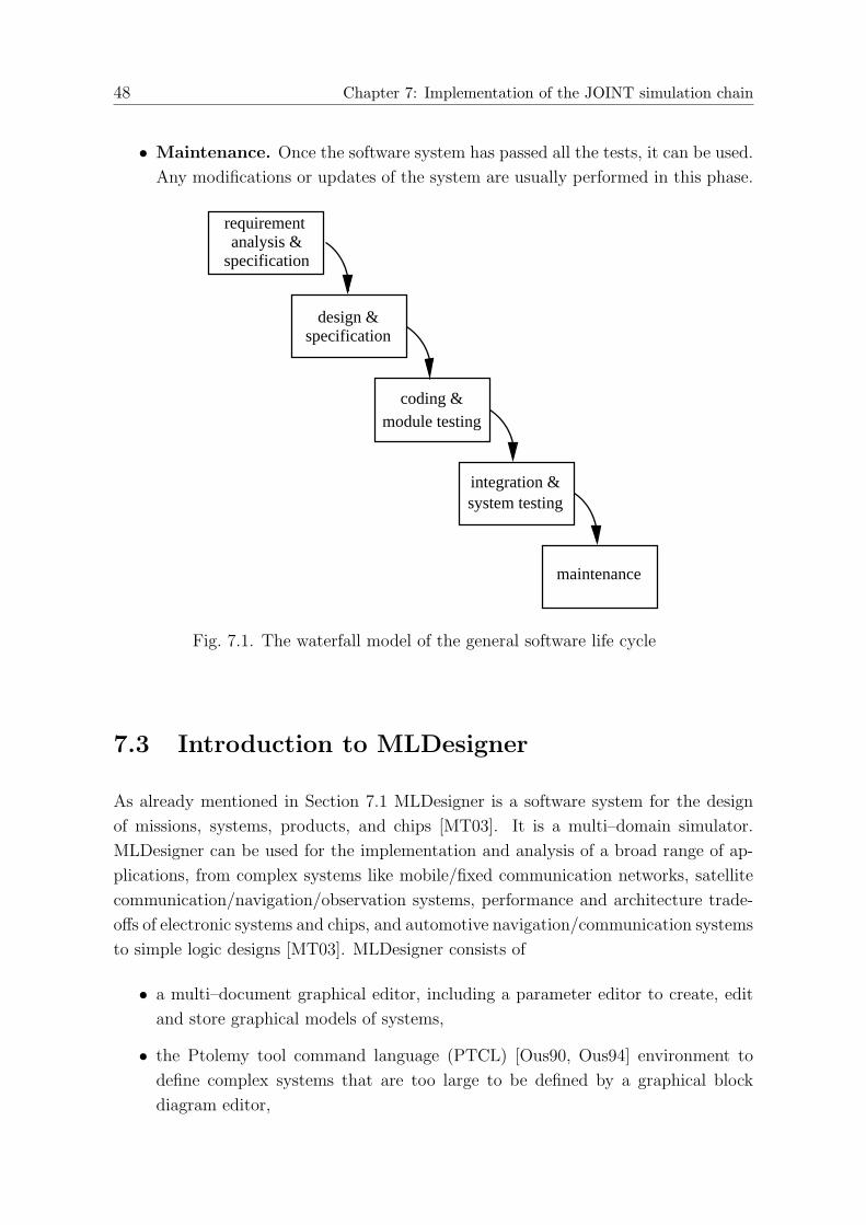
48 Chapter 7: Implementation of the JOINT simulation chain
• Maintenance. Once the software system has passed all the tests, it can be used.
Any modifications or updates of the system are usually performed in this phase.
specificationdesign &
analysis &requirement
specification
maintenance
integration &system testing
coding &module testing
Fig. 7.1. The waterfall model of the general software life cycle
7.3 Introduction to MLDesigner
As already mentioned in Section 7.1 MLDesigner is a software system for the design
of missions, systems, products, and chips [MT03]. It is a multi–domain simulator.
MLDesigner can be used for the implementation and analysis of a broad range of ap-
plications, from complex systems like mobile/fixed communication networks, satellite
communication/navigation/observation systems, performance and architecture trade-
offs of electronic systems and chips, and automotive navigation/communication systems
to simple logic designs [MT03]. MLDesigner consists of
• a multi–document graphical editor, including a parameter editor to create, edit
and store graphical models of systems,
• the Ptolemy tool command language (PTCL) [Ous90, Ous94] environment to
define complex systems that are too large to be defined by a graphical block
diagram editor,

7.3 Introduction to MLDesigner 49
• an animation and plotting system to present simulation results and performance
measures,
• integrated multi–domain simulators, including debugging animators,
• more than 1400 core modules and
• more than 260 example systems.
The functional modelling in MLDesigner is generally realized either by a network of
embedded model components or by the programming code. A model component may
define a number of ports or parameters as well as other model elements such as mem-
ories, events, and resources [MT03] to describe its external interfaces or behavior.
External interfaces are needed for embedding the model component into the functional
model of other model components. Embedding is realized by instantiating model in-
stances, i.e., the model contains references to embedded model components. This type
of hierarchical system model structure, as shown in Fig.7.2, allows embedding of mod-
ules from other domains. For a better understanding of the thesis, it is necessary to
know the following terms:
• Primitive. Primitives are the model components of the lowest level in MLDe-
signer. The functionality of a primitive is realized by using the Ptolemy
[Ous90, Ous94] language containing C++ code fragments. The model ports of a
primitive component define its external interfaces, whereas the primitive source
code written in the Ptolemy [Ous90, Ous94] language defines the behavior of the
primitive. Primitives can have input/output ports and parameters for interfacing.
They are called Stars in the Ptolemy vocabulary [Ous90, Ous94].
• Module. Modules are made up of connected embedded primitives or modules.
Like primitives, modules can have input/output ports as well as parameters for
interfacing. A module can be a simple structure with one level or a hierarchical
structure with more levels of embedded modules. Modules are called Galaxies in
the Ptolemy vocabulary [Ous90, Ous94].
• System. System is the top–level model and consists of a number of connected
primitives or modules. A system does not have any input/output ports. Defined
parameters are used to parameterize the system model. A system model is called
a Universe in the Ptolemy vocabulary [Ous90, Ous94].
As already said, MLDesigner is a multi–domain simulator. Among the diverse do-
mains Synchronous Data Flow (SDF) [MT03] is one of the most mature domains in
50 Chapter 7: Implementation of the JOINT simulation chain
Primitive
Primitive
Primitive
Module Module
Primitive
Primitive
Module
System
Fig. 7.2. Embedded structure of MLDesigner
MLDesigner, having a large amount of primitives and demo programs. Therefore, the
JOINT simulation chain is implemented in this SDF domain. The SDF domain is a
data–driven, statically scheduled domain. ”Data–driven” means that the availability
of particles at the inputs of a primitive enables the primitive. Primitives without any
inputs are always enabled. ”Statically scheduled” means that the firing order of the
primitives is determined once during the start–up phase.
7.4 Implementation of key modules of the JOINT
simulation chain
7.4.1 Preliminary remarks
In the present subsection the key primitives and modules of the JOINT simulation
chain are described. For a first overview, the key primitives and the key modules,
respectively, are listed in Tables 7.1 and 7.2.

7.4 Implementation of key modules of the JOINT simulation chain 51
Table 7.1. Key primitives of JOINT
Designation Functionality
ChannelModels Generator of CSIBitSource Generator of random binary information bitsNoise Generator of the complex Gaussian noisePilot gen Generator of the pilots for the MTsQPSK Mod QPSK modulatorQPSK DeMod QPSK demodulatorMux Multiplexer of the data and the pilotsDemux De–multiplexer the receive data and the receive pilotsJointChannelEstimation Estimator of CSIsort channels Sorter of the CTF matrix for the subcarrierwise processingJD core Detector with subcarierwise JD algorithmsJT core Transmitter with subcarierwise JT algorithmsBER Calculator of BERs
7.4.2 Channel models
7.4.2.1 Features
CSI, which is required by the data transmission and estimation, see Chapters 5 and 6,
is generated by the primitive ”ChannelModels”. The following requirements are met
according to the system design:
• The primitive ”ChannelModels” generates NB slot–specific CSI data for NB time
slots of a frame each time when the primitive is triggered.
• According to different scenarios multiple channel models are available.
• Beyond the randomly generated CSI data, the primitive ”ChannelModels” is able
to load the static CSI data from an existing file, which may be obtained by other
means. In other words, not only the living channels, but also the given snapshots
of the channels can be offered according to the desired scenario.
7.4.2.2 Particular description
As depicted in Fig.7.3, the primitive ”ChannelModels” has only one output port, which
offers the complex CSI data sequently.
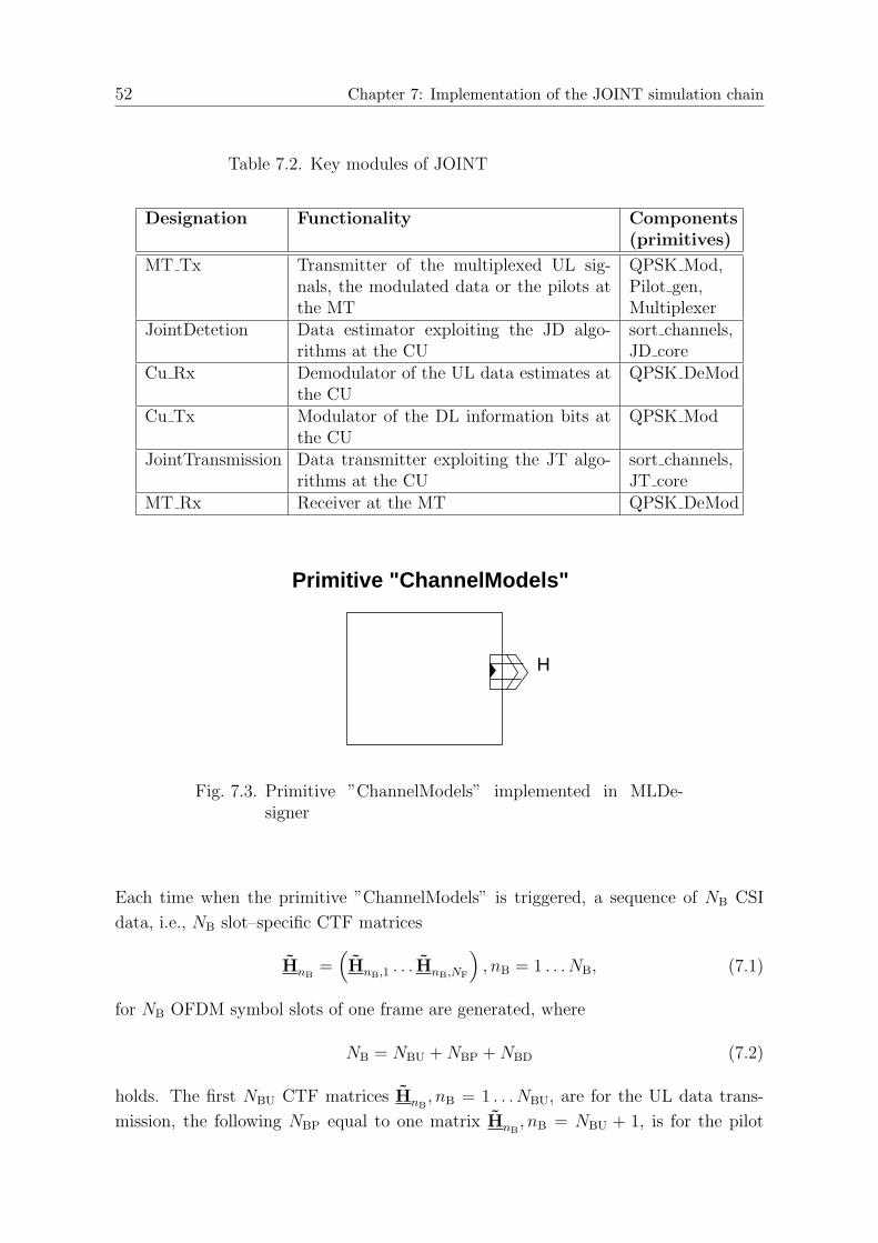
52 Chapter 7: Implementation of the JOINT simulation chain
Table 7.2. Key modules of JOINT
Designation Functionality Components(primitives)
MT Tx Transmitter of the multiplexed UL sig-nals, the modulated data or the pilots atthe MT
QPSK Mod,Pilot gen,Multiplexer
JointDetetion Data estimator exploiting the JD algo-rithms at the CU
sort channels,JD core
Cu Rx Demodulator of the UL data estimates atthe CU
QPSK DeMod
Cu Tx Modulator of the DL information bits atthe CU
QPSK Mod
JointTransmission Data transmitter exploiting the JT algo-rithms at the CU
sort channels,JT core
MT Rx Receiver at the MT QPSK DeMod
H
Primitive "ChannelModels"
Fig. 7.3. Primitive ”ChannelModels” implemented in MLDe-signer
Each time when the primitive ”ChannelModels” is triggered, a sequence of NB CSI
data, i.e., NB slot–specific CTF matrices
HnB=
(HnB,1 . . . HnB,NF
), nB = 1 . . . NB, (7.1)
for NB OFDM symbol slots of one frame are generated, where
NB = NBU + NBP + NBD (7.2)
holds. The first NBU CTF matrices HnB, nB = 1 . . . NBU, are for the UL data trans-
mission, the following NBP equal to one matrix HnB, nB = NBU + 1, is for the pilot
7.4 Implementation of key modules of the JOINT simulation chain 53
transmission in the UL, and the last NBD CTF matrices HnB, nB = NBU +2 . . . NB, are
for the DL data transmission.
The slot–specific CTF matrix HnBof (7.1) consists of NF subcarrier–specific submatri-
ces HnB,nF, each of dimensions NAP×NMT, where NAP and NMT represent the number
of the considered APs and the number of the considered MTs in the co–channel SAs,
respectively. With NSA denoting the number of the co–channel SAs in the considered
area and with the assumption of the same number KB of APs and the same number
K of MTs in each SA,
NAP = NSA ·KB (7.3)
and
NMT = NSA ·K (7.4)
hold. Consequently, the subcarrier–specific submatrix
HnB,nF=
H(1,1)
nB,nF· · · H
(1,NSA)
nB,nF...
...
H(NSA,1)
nB,nF· · · H
(NSA,NSA)
nB,nF
(7.5)
of (7.1) comprises NSA × NSA submatrices H(nSA,nSA)
nB,nF, each of dimensions KB × K,
describing all the co–channel CTFs in the considered area, which is covered by the
multiple SAs. The submatrices H(nSA,nSA)
nB,nFon the diagonal of (7.5) correspond to the
subcarrier–specific matrix Hu,nFof (3.20) in the UL or the transpose of the subcarrier–
specific matrix HT
d,nFof (3.28) in the DL in the corresponding SAs., i.e.,
H(nSA,nSA)
nB,nF= Hu,nF
= HT
d,nF. (7.6)
The single–SA scenario is a special case of NSA equal to one. With (7.3) and (7.4)
NAP = KB (7.7)
and
NMT = K (7.8)
can be obtained for NSA equal to one.
The elements of the slot–specific CTF matrix HnBof (7.1) can be generated according
to the algorithms in Chapter 2 for different types of channel models. The types of the
channel models can be chosen by setting the parameter ”chan type”. Different integer
values of ”chan type” correspond to the basic channel models, e.g., ”1” representing
for a non–cross–coupling channel model, in which
HnB,nF= IK (7.9)

54 Chapter 7: Implementation of the JOINT simulation chain
holds, ”2” presenting a Rayleigh fading channel model with an exponential power delay
profile and a Jakes Doppler spectrum [Ste92, Pro95, LR99] as introduced in Subsection
2.3.1, ”3” representing a Rayleigh fading channel model with log–normal fading as
described in Subsection 2.3.2, and ”4” representing a channel model loaded from an
existing file.
For the other parameters concerning the channel models and JOINT, which are con-
sistent with the ones used in Chapters 2 and 3, refer to Table 3.1.
7.4.3 Joint channel estimation
7.4.3.1 Features
The task of the primitive ”JointChannelEstimation” is to offer the desired CSI data
for the data estimation in the UL and the data transmission in the DL, as stated in
Chapter 4. The following requirements are met according to the system design:
• The primitive ”JointChannelEstimation” delivers NB slot–specific CSI data for
NB OFDM symbol slots of a frame each time when the primitive is triggered.
• For different purposes of investigations the primitive ”JointChannelEstimation”
is able to offer either the estimated CSI data or the true CSI data.
• Both single–SA scenarios and multiple–SA scenarios can be handled.
7.4.3.2 Particular description
The primitive ”JointChannelEstimation” has two input ports, see Fig. 7.4. One in-
put port is e, which is a multiple–input port for complex matrices. Therefore, NF
subcarrier–specific receive pilot vectors
eh,nF=
(e(1)h,nF
. . . e(NAP)h,nF
)T
, (7.10)
each of dimension NAP, can be collected in a parallel manner. As depicted in Fig.7.4,
the other input port is H, which is a port for a single complex matrix. The total CTF
matrix
H =
H1...
HNB
(7.11)
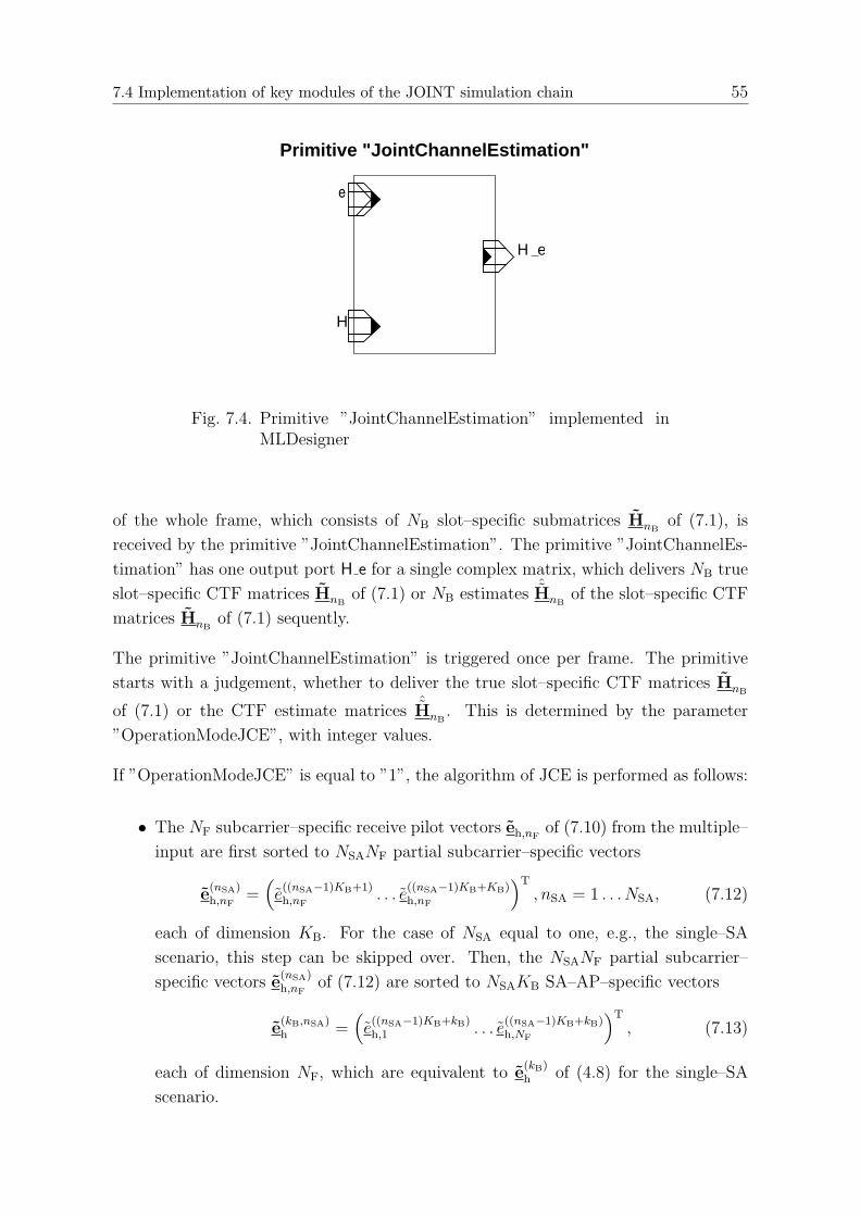
7.4 Implementation of key modules of the JOINT simulation chain 55
H_e
e
HH
e
Primitive "JointChannelEstimation"
Fig. 7.4. Primitive ”JointChannelEstimation” implemented inMLDesigner
of the whole frame, which consists of NB slot–specific submatrices HnBof (7.1), is
received by the primitive ”JointChannelEstimation”. The primitive ”JointChannelEs-
timation” has one output port H e for a single complex matrix, which delivers NB true
slot–specific CTF matrices HnBof (7.1) or NB estimates ˆHnB
of the slot–specific CTF
matrices HnBof (7.1) sequently.
The primitive ”JointChannelEstimation” is triggered once per frame. The primitive
starts with a judgement, whether to deliver the true slot–specific CTF matrices HnB
of (7.1) or the CTF estimate matrices ˆHnB. This is determined by the parameter
”OperationModeJCE”, with integer values.
If ”OperationModeJCE” is equal to ”1”, the algorithm of JCE is performed as follows:
• The NF subcarrier–specific receive pilot vectors eh,nFof (7.10) from the multiple–
input are first sorted to NSANF partial subcarrier–specific vectors
e(nSA)h,nF
=(e((nSA−1)KB+1)h,nF
. . . e((nSA−1)KB+KB)h,nF
)T
, nSA = 1 . . . NSA, (7.12)
each of dimension KB. For the case of NSA equal to one, e.g., the single–SA
scenario, this step can be skipped over. Then, the NSANF partial subcarrier–
specific vectors e(nSA)h,nF
of (7.12) are sorted to NSAKB SA–AP–specific vectors
e(kB,nSA)h =
(e((nSA−1)KB+kB)h,1 . . . e
((nSA−1)KB+kB)h,NF
)T
, (7.13)
each of dimension NF, which are equivalent to e(kB)h of (4.8) for the single–SA
scenario.
56 Chapter 7: Implementation of the JOINT simulation chain
• Secondly, the SA–AP–specific receive pilot vectors e(kB,nSA)h of (7.13) are pro-
cessed, respectively, for the corresponding SA nSA, nSA = 1 . . . NSA, according to
(4.16) to (4.18). Therefore, the SA–AP–specific CTF estimate vectors ˆh(kB,nSA),
which are equivalent to ˆh(kB) of (4.18) in the case of the single–SA scenario, each
of dimension KNF, can be obtained.
• Thirdly, the estimate ˆHnBof the slot–specific CTF matrix HnB
of (7.1) for the
time slot nB equal to NBU + 1, which is reserved for the pilot transmission, can
be constructed with the NSAKB SA–AP–specific CTF estimate vectors ˆh(kB,nSA).
Since it is assumed that the channels are time invariant during one transmission
frame, NB replicas of the slot–specific CTF estimate matrix ˆHNBU+1 at the time
slot nB equal to NBU + 1 are delivered sequently at the output port H e.
If ”OperationModeJCE” is equal to ”0”, the algorithm of JCE is not performed. The
total CTF matrix H of (7.11) is simply sorted into NB sequent slot–specific CTF
matrices HnBof (7.1). The NB matrices HnB
of (7.1), which may differ from each
other, are delivered sequently at the output port H e.
The parameter ”PilotType” indicates which type of pilots is used, corresponding to the
type of pilots applied in the MTs. Different integer values correspond to the different
types of pilots. In the following investigations, the pilots based on Walsh codes, as
introduced in Section 4.4, are considered. Concerning the other parameters related to
JCE, e.g., the channel dimension W and the pilot energy Ep, these parameters are
consistent with the ones used in Chapter 4.
7.4.4 Joint detection
7.4.4.1 Features
The whole task of the data estimation in the UL is undertaken by the module ”Joint-
Dection”. The prerequisites of JD are the known CSI data in terms of the CTF
matrices HnBof (7.1), which are offered by the primitive ”JointChannelEstimation”
as discussed in Subsection 7.4.3. The following requirements are met according to the
system design:
• The linear JD algorithms are realized in the module ”JointDection”.
• Subcarrierwise processing for the linear JD algorithms is favored.
• The extension to some nonlinear JD algorithms is possible.
• Both single–SA scenarios and multiple–SA scenarios can be handled.

7.4 Implementation of key modules of the JOINT simulation chain 57
7.4.4.2 Particular description
The module ”JointDection”, consisting of two functional components, i.e., the primitive
”sort channel” and the primitive ”JD core”, as depicted in Fig.7.5, is processed NBU
times per frame. The module ”JointDection” has two input ports. One input port is
e, which is a multiple–input port for complex matrices. Therefore, NF slot–subcarrier–
specific receive data vectors
eu,nB,nF=
(e(1)u,nB,nF
. . . e(NAP)u,nB,nF
)T, (7.14)
each of dimension NAP equal to NSAKB, can be collected in parallel for the time slot
nB, nB = 1 . . . NBU. In the case of NSA equal to one, i.e., the single–SA scenario,
the slot–subcarrier–specific receive data vectors eu,nB,nFof (7.14) are equivalent to the
subcarrier–specific receive data vectors eu,nFof (3.20), each of dimension KB. The
other input port is H, which is for a single complex matrix. Through the port H the
slot–specific CTF matrices HnBof (7.1) are delivered sequently, for the corresponding
time slot nB in the UL transmissions. The module ”JointDection” has one output port
d e, which is a multiple–output port for complex matrices. Through the port d e NF
slot–subcarrier–specific data estimate vectors
ˆdu,nB,nF=
(ˆd(1)
u,nB,nF. . . ˆd(NMT)
u,nB,nF
)T
, (7.15)
each of dimension NMT equal to NSAK, are delivered for the time slot nB. In the case
of NSA equal to one, i.e., the single–SA scenario, ˆdu,nB,nFof (7.15) is equivalent to the
subcarrier–specific data estimate vectors ˆdu,nFof (5.2), each of dimension K.
The primitive ”sort channel” aims at sorting the slot–specific CTF matrix HnBof
(7.1) into a slot–subcarrier–specific form HnB,nFof (7.1), which are desired by the
subcarrierwise JD algorithms, for the time slot nB. The input port of the primitive
”sort channel” is connected to the input port H of the module ”JointDetection”. The
output port of the primitive ”sort channel”, which is a multiple–output port for com-
plex matrices, is connected to one of the input ports of JD core so that the NF sorted
slot–subcarrier–specific CTF matrices HnB,nFof (7.1) are delivered in parallel to the
primitive ”JD core” at the time slot nB.
The primitive ”JD core” accomplishes the key JD algorithms. The primitive ”JD core”
has two input ports. Both input ports are multiple–input ports for complex matrices.
One input port is connected directly to the input port e of the module ”JointDetection”
to receive the NF parallel slot–subcarrier–specific receive data vectors eu,nB,nFof (7.14),
each of dimension NSAKB. The other input port is connected to the output port of
the primitive ”sort channel” for the NF slot–subcarrier–specific CTF matrices HnB,nF

58 Chapter 7: Implementation of the JOINT simulation chain
sort_channel
JD_core
e
H
d_e
$N_F
Joint Detection module
sort channel matrix subcarrier wise
H
Module "JointDetection"
ed_e
Fig. 7.5. Module ”JointDection” implemented in MLDesigner
of (7.1). The output port d e of the primitive ”JD core” is a multiple–output port for
complex matrices. The primitive ”JD core” works as follows:
• Firstly, the NF slot–subcarrier–specific receive data vectors eu,nB,nFof (7.14) are
sorted to NSANF partial slot–subcarrier–specific receive data vectors
e(nSA)u,nB,nF
=(e((nSA−1)KB+1)u,nB,nF
. . . e((nSA−1)KB+KB)u,nB,nF
)T, (7.16)
each of dimension KB.
• Then, the NF slot–subcarrier–specific CTF matrices HnB,nFof (7.1) are sorted
so that NSANF SA–slot–subcarrier–specific CTF matrix H(nSA,nSA)
nB,nFof (7.5), each
of dimensions KB ×K, which are actually the diagonal submatrices of HnB,nFof
(7.5), are obtained.
• Thirdly, according to the JD algorithms discussed in Chapter 5, two options
are available: the RxMF JD and the RxZF JD. The parameter ”detector type”
determines which type of the joint detectors is applied. The SA–slot–subcarrier–
specific data estimate vectors ˆd(nSA)
u,nB,nFcan be obtained with (5.8) for the RxMF
JD, or with (5.11) for the RxZF JD, respectively.

7.4 Implementation of key modules of the JOINT simulation chain 59
• The NSANF SA–slot–subcarrier–specific data estimate vectors ˆd(nSA)
u,nB,nF, each of
dimension K, are sorted to NF slot–subcarrier–specific data estimate vectorsˆdu,nB,nF
of (7.15), each of dimension NSAK.
For single–SA scenarios, the process described above can be simplified by setting NSA
equal to one.
7.4.5 Joint transmission
7.4.5.1 Features
The task of the data transmission in the DL is undertaken by the module ”Joint-
Transmission”. The prerequisites of JT are the known CSI data in terms of the CTF
matrices HnBof (7.1), which are offered by the primitive ”JointChannelEstimation”
as discussed in Subsection 7.4.3. The following requirements are met according to the
system design:
• The linear JT algorithms are realized in the module ”JointTransmission”.
• Subcarrierwise processing for the linear JT algorithms is favored.
• The extension to some nonlinear JT algorithms is possible.
• Both single–SA scenarios and multiple–SA scenarios can be handled.
7.4.5.2 Particular description
The module ”JointTransmission”, consisting of the primitive ”sort channel” and the
primitive ”JT core”, as depicted in Fig.7.6, is processed NBD times per frame. The
module ”JointTransmission” has two input ports. One input port is d, which is a
multiple–input port for complex matrices. Therefore, NF slot–subcarrier–specific trans-
mit data vectors
dd,nB,nF=
(d
(1)
d,nB,nF. . . d
(NMT)
d,nB,nF
)T
, (7.17)
each of dimension NMT, can be sent in parallel for the time slot nB, nB = NBU+2 . . . NB.
In the case of NSA equal to one, i.e., the single–SA scenario, the slot–subcarrier–
specific transmit data vectors dd,nB,nFof (7.17) are equivalent to the subcarrier–specific
transmit data vector dd,nFof (6.1), each of dimension K. The other input port is H,

60 Chapter 7: Implementation of the JOINT simulation chain
sort channel
JT_core
d
H
t
$N_F
Joint Transmission module
sort channel matrix subcarrier wise
d
H
Module "JointTransmission"
t
Fig. 7.6. Module ”JointTransmission” implemented in MLDe-signer
which is for a single complex matrix. Through the port H the DL slot–specific CTF
matrices HT
nBare delivered sequently at the time slot nB for the DL transmissions. The
module ”JointTransmission” has one output port t, which is a multiple–output port
for complex matrices. Through the port t NF slot–subcarrier–specific transmit vectors
sd,nB,nF=
(s(1)d,nB,nF
. . . s(NAP)d,nB,nF
)T
, (7.18)
each of dimension NAP equal to NSAKB, are delivered for the time slot nB. In the case
of NSA equal to one, i.e., the single–SA scenario, sd,nB,nFof (7.18) is equivalent to the
subcarrier–specific transmit vector sd,nFof (3.28), each of dimension KB.
The primitive ”sort channel” aims at sorting the DL slot–specific CTF matrix HT
nB
into a slot–subcarrier–specific form HT
nB,nF, which is desired by the subcarrierwise JT
algorithms for the time slot nB. The input port of the primitive ”sort channel” is
connected to the input port H of the module ”JointTransmission”. The output port of
the primitive ”sort channel”, which is a multiple–output port for complex matrices, is
connected to one of the input ports of the primitive ”JT core” so that the NF sorted
DL slot–subcarrier–specific CTF matrices HT
nB,nFof (7.1) are delivered in parallel to
the primitive ”JT core”.

7.4 Implementation of key modules of the JOINT simulation chain 61
The primitive ”JT core” accomplishes the key JT algorithms. The primitive ”JT core”
has two input ports. Both input ports are multiple–input ports for complex matrices.
One input port is connected directly to the input port d of the module ”JointTransmis-
sion” to receive NF parallel slot–subcarrier–specific data vectors dd,nB,nFof (7.17) to
be transmitted, each of dimension NSAK. The other input is connected to the output
port of the primitive ”sort channel” for the NF slot–subcarrier–specific CTF matrices
HT
nB,nF. The output port t of the primitive ”JT core” is a multiple–output port, which
delivers NF slot–subcarrier–specific transmit vectors sd,nB,nFof (7.18). The primitive
”JT core” works as follows:
• Firstly, the NF slot–subcarrier–specific data vectors dd,nB,nFof (7.17) to be trans-
mitted are sorted to NSANF partial slot–subcarrier–specific data vectors
d(nSA)
d,nB,nF=
(d
((nSA−1)K+1)
d,nB,nF. . . d
((nSA−1)K+K)
d,nB,nF
)T
, (7.19)
each of dimension K.
• Then, the NF slot–subcarrier–specific CTF matrices HT
nB,nFin the DL trans-
mission are sorted so that NSANF SA–slot–subcarrier–specific CTF matrix
H(nSA,nSA)
nB,nF
T
in the DL, each of dimensions K ×KB, which are actually the trans-
pose of the diagonal submatrices of HnB,nFof (7.5), are obtained.
• Thirdly, two options, the TxMF JT and the TxZF JT, are available according
to the two JT algorithms discussed in Chapter 6. The parameter ”transmit-
ter type” determines which type of the joint transmitters is applied. The SA–
slot–subcarrier–specific modulator matrix M(nSA)
nB,nFcan be obtained with (6.11)
for the TxMF JT, or with (6.14) for the TxZF JT, respectively. Therefore, the
SA–slot–subcarrier–specific transmit vectors
s(nSA)d,nB,nF
=(s((nSA−1)KB+1)d,nB,nF
. . . s((nSA−1)KB+KB)d,nB,nF
)T
, (7.20)
each of dimension KB, can be obtained.
• The NSANF SA–slot–subcarrier–specific transmit vectors s(nSA)d,nB,nF
of (7.20), are
sorted to NF slot–subcarrier–specific data estimate vectors sd,nB,nFof (7.18).
For single–SA scenarios, the process described above can be simplified by setting NSA
equal to one.

62 Chapter 7: Implementation of the JOINT simulation chain
7.5 Implementation of the JOINT simulation chain
Concerning the physical layer (PHY) investigation in conventional cellular systems,
link level and system level performances [Ste96, Lu01] are usually jointly considered.
However, in the SA based system JOINT, things become different and complicated,
mainly in the system level investigation. For instance in the UL, since APs in a SA
are distributed away from each other, the interferences received at the different APs
differ from each other so that the signal–to–noise–and–interference ratios (SNIRs) at
the different APs become variable as well, even when the noise power is given to be
the same. On the other hand, in the DL the data transmission signals are strictly
designed by the JT algorithms. Therefore, it is problematic to calculated the exact
interferences at the MTs without the knowledge about the detailed transmission in
other co–channel SAs. In one word, it is very difficult to do the system level simulations
with power control schemes in the SA based system as compared in the conventional
cellular system.
In this thesis, the end–to–end performance investigation of JOINT, in terms of BERs,
is focused on. Therefore, a simulation chain of JOINT for the BER simulation is
implemented, as depicted in Fig. 7.7. The JOINT simulation chain for the system
level investigations is not included in the thesis. The link level JOINT simulation
chain comprises the UL part and the DL part, which are associated by the reciprocal
channels.
In the UL part, a complete link consists of
• the primitive ”BitSource”, an information–bit generator which generates the bi-
nary sequences in parallel for the multiple MTs,
• the module ”MT Tx”, a transmitter of the MT which includes a modulator, a
pilot generator and a data–pilot multiplexer for each MT,
• the primitive ”Noise UL”, a noise generator which generates the Gaussian noise
in the UL,
• the primitive ”ChannelModels” introduced in Subsection 7.4.2,
• the primitive ”Chan UL”, which realizes the UL process, in which signals are
distorted by a linear transmission system and the noise,
• the primitive ”Demux”, a de–multiplexer which distinguishes the pilot and the
data transmission for the following the primitive ”JointChannelEstimation” and
the module ”JointDetection”, introduced in Subsections 7.4.3 and 7.4.4, respec-
tively,

7.5 Implementation of the JOINT simulation chain 63
• the module ”CU Rx”, a demodulator and
• the primitive ”BER”, a BER calculator, which compares the estimate bits and
the data bits and calculates the BERs for the corresponding MTs.
In the DL part, a complete link consists of
• the primitive ”BitSource”, an information–bit generator which is the same as the
one in the UL part,
• the module ”CU Tx”, a transmitter of the CU which realizes the signal modula-
tion for each MT,
• the module ”JointTransmission” as introduced in 7.4.5,
• the primitive ”Noise DL”, a noise generator which generates the Gaussian noise
in the DL,
• the primitive ”Chan DL”, a primitive which realizes the DL process, in which
signals are distorted by a linear transmission system and the noise,
• the module ”MT Rx”, a demodulator and
• the primitive ”BER”, a BER calculator which compares the estimate bits and
the data bits and calculates the BERs for the corresponding MTs.
There are some other primitives like e.g., ”form”/ ”re–form”, ”Park”, ”switchA”/
”switchB”/ ”switchC” and ”UL 2 DL”, which realize the important roles forming the
desired structures for input ports of the other functional primitives or modules without
changing the values of the particles, where the particles indicate any data flowing
through primitives and/or modules of a system, including e.g., data bits and data
symbols in the form of scalars or of vectors/matrices [MT03].
By setting the proper parameters, the JOINT simulation chain, as shown in Fig.7.7,
can be run for single–/multiple–SA scenarios, for different channel models, and for
some other different system requirements.

64 Chapter 7: Implementation of the JOINT simulation chain
7.6 Specific problems and solutions
7.6.1 Synchronization
The topic on synchronization of JOINT has been considered in Section 3.3. Here,
the problem of synchronization among the modules and the primitives of the JOINT
simulation chain is addressed.
As stated in Section 7.3, most of the primitives and modules are designed and imple-
mented in the SDF domain. One basic principle in the SDF domain is the balance
between the produced particles and the consumed particles [MT03].
Each port of an SDF primitive has an attribute that specifies the number of particles
consumed for input ports or the number of particles produced for output ports [MT03].
When an input port is connected to an output port with an arc, the number of particles
produced on the arc by the source primitive may not be the same as the number of
particles consumed from that arc by the destination primitive. To maintain a balanced
system, the scheduler must fire the source and destination primitives with different
frequencies.
The primitive ”JointChannelEstimaiton” is a good example to show how the balance
is kept. The primitive ”JointChannelEstimaiton” is processed once per frame exactly
at the time slot nB equal to NBU +1 for the pilot transmission. However, the primitive
”JointChannelEstimaiton” has to receive all the CSI data of the NB time slots in the
whole frame in order to fulfill the design requirement of delivering the true CSI data
as well as the CSI estimates for JD in the UL and for JT in the DL. Such a confliction
can be solved by some tricks to keep the system in balance. At the input port H of the
primitive ”JointChannelEstimaiton” the NB slot–specific CTF matrices HnBof (7.1)
should be be loaded together in the form of a new big matrix H of (7.11) at the time
slot nB equal to NBU + 1 when the primitive ”JointChannelEstimaiton” is triggered.
This means between the channel model primitive and the primitive ”JointChannelEs-
timaiton” there should exist a primitive named ”Park”, as depicted in Fig. 7.7, in
which the sequent slot–specific CTF matrices HnBof (7.1) sent out at the output
port H of the channel model primitive are detained and sorted into a big matrix H
of (7.11) delivered to the input port H of the primitive ”JointChannelEstimaiton”.
On the other hand the NB sequent slot–specific matrices HnBof (7.1) will be de-
livered from the output port H e of the primitive ”JointChannelEstimaiton” to the
output port H of the module ”JointDetection” and to the output port H of the mod-
ule ”JointTransmission”. However, only the first NBU slot–specific CTF matrices HnB
of (7.1) are required by the module ”JointDetection”, and the last NBD slot–specific

7.6 Specific problems and solutions 65
CTF matrices HnBof (7.1) are required by the module ”JointTransmission”, respec-
tively. Therefore, between the primitive ”JointChannelEstimaiton” and the modules
”JointDetection”/”JointTransmission”, there should exist a primitive ”Switch”, as de-
picted in Fig. 7.7, in which the NB sequent slot–specific CTF matrices HnBof (7.1)
are handled so that the first NBU slot–specific CTF matrices HnBof (7.1) and the last
NBD slot–specific CTF matrices HnBof (7.1) are delivered separately. This means one
slot–specific CTF matrix HnBof (7.1) at the time slot nB equal to NBU+1 is discarded.
7.6.2 Simulation efficiency
The JOINT simulation consists of many modules and primitives. Great amounts of
calculations are carried out when simulations are running. Therefore, the CPU and
memory of a computer system are greatly occupied during the simulations. Especially
concerning the memory, if the memory consumption of the simulation chain is too high
and exceeds the upper limit of the tolerance of the computer system, the simulation
will be blocked or even cancelled. In order to avoid this, we have to carefully design
the system to make an efficient use of the memory.
One way is to optimize the algorithms during the implementation. For instance in
the JCE algorithm, the matrix Z of (4.18), only depends on the pilot matrix P of
(4.16) and the matrix FW,tot of (4.18), as discussed in Section 4.3. Meanwhile, the pilot
matrix P of (4.16) and the matrix FW,tot of (4.18) are fixed once the parameters K, W
and NF are determined. Therefore, the matrix Z of (4.18) is constant throughout the
simulation once the parameters K, W and NF are fixed. This means, that the matrix
Z of (4.18) needs to be calculated only once during the simulation in the optimized
JCE algorithm. Such a modification can be achieved by putting the part of codes for
the Z calculation into the ”begin” method in stead of the ”go” method, where the
term method is a term of C++ programs indicating a paragraph of codes for the given
functionality. The method ”begin” is to be executed only once at the very beginning
after the total system is successfully compiled and properly scheduled. However, the
method ”go” is to be executed each time when the primitive is triggered. Consequently,
the computational effort and the memory consumption are greatly reduced.
Another way to improve the memory efficiency is to avoid memory leaks. Most primi-
tives deal with matrices. Therefore, allocating memory space to these matrices during
the calculation is necessary. Memory leaks occur when new memory space is allocated
dynamically and never deallocated. In C programs, new memory space is allocated by
the functions ”malloc” or ”calloc”, and deallocated by the function ”free”. In C++,
new memory space is usually allocated by the operator ”new” and deallocated by the

66 Chapter 7: Implementation of the JOINT simulation chain
operator ”delete”. The problem with memory leaks is that the memory space, which is
not deallocated after being used, accumulates over time and may cripple or even crash
a program. The operator ”cleanup” should be applied to variables containing dynamic
memory. Some common mistakes may lead to memory leaks, like, e.g., the improper
usage of the operator ”delete” and overwriting a variable containing dynamic memory
without freeing any existing memory first. Besides carefully checking the codes, the
following two tricks can be used:
• In the method ”constructor” of a primitive, the variables containing dynamic
memory should be initialized to zero.
• By freeing memory apply the method ”cleanup”, which covers all possible cases
of memory leaks during simulations.

7.6 Specific problems and solutions 67
CU_R
xMT_Tx
Bit Source
Chan UL
Dem
uxJD switchB
Channel Model
switchA
Bit Source
CU_Tx
Chan DL
MT_Rx
form
re-form
form
re-form
JCE
Pack
UL 2 DL
UL 2 DL
JT
Noise_UL
Pack
Noise_DL
Pack
BER
BER
$K
$N_F
$K
$K
$N_F
$N_F
$K
$K
$N_F
$K
$N_F
$N_F
$N_F
$N_F
$N_F
$N_F
$N_F
$N_F
$K
$K
$K
$K
JOIN
T si
mul
atio
n ch
ain
(on
link
leve
l)
Fig. 7.7. JOINT simulation chain in MLDesigner

68
Chapter 8
Performance of JOINT in asingle–service–area scenario
8.1 Preliminary remarks
The main advantage of the SA based JOINT compared to conventional cellular systems
is that JOINT is capable to combat the intra–SA MAI and to improve the system
performance, as explained in Chapter 1. In the present chapter, the system performance
of JOINT will be evaluated in a single–SA scenario, in which the inter–SA MAI is
temporarily ignored. Therefore, the performance of the data estimation technique and
the data transmission technique of JOINT in the noise–limited case can be focused on.
In the present chapter, first the duality between the UL and the DL of JOINT is
discussed under the assumption of perfect CSI. A general model of the linear data
transmission is given. The UL performance and the DL performance, in terms of bit
error probabilities, are compared on the basis of this general model so that the duality
of the UL and the DL performances can be deduced. Moreover, this performance
duality is also analyzed with respect to the efficiency of energy transmission.
CSI is the prerequisite for the data estimation in the UL and the data transmission in
the DL. However, the CSI estimation errors are inevitable if JCE is applied. Two major
factors, which lead to the CSI estimation errors, are analyzed. In the present chapter,
the influences of the CSI estimation errors on the UL and the DL performances are
also discussed.
Finally, numerical results obtained with the JOINT simulation chain introduced in
Chapter 7 are given to demonstrate the aforementioned analysis.
8.2 Duality of the uplink and the downlink perfor-
mances
8.2.1 General model of linear data transmission
In order to deeply understand the intrinsic relation between the UL transmission and
the DL transmission of JOINT, it is necessary to study a more general linear data

8.2 Duality of the uplink and the downlink performances 69
transmission first, which covers all the common characteristics of the UL transmission
and the DL transmission.
HnFDnF
ˆdnF
nnF
enFsnF
dnF
MnF
Fig. 8.1. General subcarrierwise model of a linear transmission
Fig. 8.1 shows such a general model of the linear data transmission in the frequency
domain with respect to the subcarrier nF [Skl04], regardless of the UL or the DL. The
data vector
dnF=
(d
(1)
nF. . . d
(K)
nF
)T
(8.1)
of dimension K is first pre–processed by a linear modulator matrix MnFof dimensions
KI×K, where KI denotes the number of the inputs of the MIMO channel. Therefore,
the transmit vector
snF=
(s(1)
nF. . . s(KI)
nF
)T(8.2)
of dimension KI can be generated by multiplying the data vector dnFof (8.1) by the
modulation matrix MnF, i.e.,
snF= MnF
dnF. (8.3)
Then, the transmit vector snFof (8.2) is fed into the MIMO channel denoted by the
CTF matrix HnFof dimensions KO×KI, where KO denotes the number of the outputs
of the MIMO channel. The transmit vector snFof (8.2) is corrupted by the noise,
which is denoted by the noise vector
nnF=
(n(1)
nF. . . n(KO)
nF
)T(8.4)
of dimension KO. Therefore, the receive vector
enF=
(e(1)
nF. . . e(KO)
nF
)T(8.5)
of dimension KO can be obtained by
enF= HnF
snF+ nnF
. (8.6)
The receive vector enFof (8.5) is processed by a linear detection process mathematically
described by the detector matrix DnFof dimensions K × KO so that with (8.3) and
(8.6) the data estimate vector
ˆdnF=
(ˆd(1)
nF. . . ˆd(K)
nF
)T
(8.7)

70 Chapter 8: Performance of JOINT in a single–service–area scenario
of dimension K is given by
ˆdnF= DnF
enF
= DnFHnF
MnFdnF
+ DnFnnF
. (8.8)
It is assumed that the uncorrelated data symbols d(k)
nFhave equal energies
Ed =1
2|d(k)
nF|2, k, 1 . . . K. (8.9)
For the covariance matrix of the data vector dnFof (8.1) follows
Rd = E{dnF
d∗TnF
}= 2Ed · IK . (8.10)
With σ2 denoting the variance of real and imaginary parts of the uncorrelated noise
elements n(kO)nF
of (8.4), the covariance matrix of the noise vector nnFof (8.4) reads
Rn = E{
nnFn∗TnF
}= 2σ2 · IKO . (8.11)
According to (6.10) the transmit energy
T (k)nF
=1
2|d(k)
nF|2
[M
∗TnF
MnF
]k,k
= Ed ·[M
∗TnF
MnF
]k,k
(8.12)
invested for the data symbol d(k)
nFof (8.1) is obtained. The ratio
Ed
T(k)nF
=1[
M∗TnF
MnF
]k,k
(8.13)
of the desired energy Ed of (8.9) to the transmit energy T(k)nF of (8.12) tells us how
efficiently the energy T(k)nF of (8.12) is transmitted for the data symbol d
(k)
nFof (8.1) with
the energy Ed of (8.9). Generally, the ratio Ed/T(k)nF of (8.13) is a positive value no
greater than one.
In order to obtain the unbiased data estimate ˆdnFof (8.8),
DnFHnF
MnF= IK (8.14)
has to be fulfilled so that (8.8) can be rewritten as
ˆdnF= dnF
+ DnFnnF
. (8.15)

8.2 Duality of the uplink and the downlink performances 71
The filtered noise DnFnnF
accounts for the data estimation error
∆nF= ˆdnF
− dnF= DnF
nnF. (8.16)
With (8.10), (8.11) and the assumption that the data vector dnFof (8.1) and the noise
vector nnFof (8.4) are statistically independent, the covariance matrix of the data
estimation error ∆nFof (8.16) reads
R∆ = E{∆nF
∆∗TnF
}= 2σ2
(DnF
D∗TnF
). (8.17)
With (8.10) and (8.17) the SNR
γ(k)nF
=12|d(k)
nF|2
12|ˆd(k)
nF− d
(k)
nF|2
=Ed
σ2[DnF
D∗TnF
]k,k
(8.18)
of the data symbol d(k)
nFof (8.1) can be obtained.
8.2.2 Bit error probability
In the UL of JOINT, since it is assumed that MTs and APs are equipped with single
antennas,
KI = K (8.19)
and
KO = KB (8.20)
hold. From the viewpoint of the receiver side, i.e., at the CU, the modulator matrix
MnFof (8.3) and the CTF matrix HnF
of (8.6) are a priori known. To keep the MT
structure as simple as possible is one target of the system design. Therefore, simple
OFDM transmitters are assumed to be used at the MTs, i.e., the modulator matrix
Mu,nF= IK (8.21)
holds for the UL. For the UL CTF matrix, refer to the CTF matrix Hu,nFof (3.20)
with dimensions KB ×K.
For the unbiased data estimation fulfilling (8.14), the linear RxZF JD [Kle96, Skl04]
algorithm is applied at the CU in the UL of JOINT. The linear RxZF JD [Kle96, Skl04]

72 Chapter 8: Performance of JOINT in a single–service–area scenario
minimizes the square error ‖eu,nF− Hu,nF
ˆdu,nF‖2 of the reconstructed receive signal
Hu,nF
ˆdu,nF. Therefore, with (8.14) and (8.21) the UL detector matrix
Du,nF=
((Hu,nF
Mu,nF
)∗T (Hu,nF
Mu,nF
))−1 (Hu,nF
Mu,nF
)∗T
=(M
∗Tu,nF
H∗Tu,nF
Hu,nFMu,nF
)−1
M∗Tu,nF
H∗Tu,nF
=(H∗Tu,nF
Hu,nF
)−1
H∗Tu,nF
(8.22)
can be derived. According to (8.12) and (8.21) the transmit energies
T (k)u,nF
= Ed (8.23)
invested for the data symbols d(k)
u,nFof (8.1) in the UL are equal. With (8.18), (8.22)
and (8.23) the SNR
γ(k)u,nF
=Ed
σ2[Du,nF
D∗Tu,nF
]k,k
=T
(k)u,nF
σ2
[(H∗Tu,nF
Hu,nF
)−1]
k,k
(8.24)
of the data symbol d(k)
u,nFof (8.1) in the UL is obtained. For the QPSK modulation, if the
noise elements n(k)u,nF
of (8.4) are complex Gaussian variables, the bit error probability
P(k)b,u,nF
=1
2erfc
√γ
(k)u,nF
2=
1
2erfc
√√√√√√T
(k)u,nF
σ2[(H∗Tu,nF
Hu,nF
)−1]
k,k
(8.25)
of the data symbol d(k)
u,nFof (8.1) in the UL is derived as a function of the pseudo SNR,
i.e., the transmit–energy–to–noise–power ratio T(k)u,nF/σ2 in the UL and the UL CTF
matrix Hu,nFof (3.20).
In the DL of JOINT, due to the application of single antennas on MTs and APs,
KI = KB (8.26)
and
KO = K (8.27)
hold. From the viewpoint of the transmitter side, i.e., at the CU, the detector matrix
DnFof (8.7) and the CTF matrix HnF
of (8.6) are a priori known. As in the UL, also

8.2 Duality of the uplink and the downlink performances 73
in the DL, the MT structure has to be kept as simple as possible. Therefore, simple
OFDM receivers are assumed to be used at the MTs, i.e., for the DL detector matrix
follows
Dd,nF= IK . (8.28)
For the DL CTF matrix, refer to the CTF matrix Hd,nFof (3.28) with dimensions
K ×KB, which is the transpose of the UL CTF matrix Hu,nFof (3.20).
For the unbiased data transmission fulfilling (8.14), the linear TxZF JT [MBW+00,
TWMB01, Skl04] algorithm is applied at the CU in the DL of JOINT. With (8.14) and
(8.28) the DL modulator matrix
Md,nF=
(Dd,nF
Hd,nF
)∗T ((Dd,nF
Hd,nF
)(Dd,nF
Hd,nF
)∗T)−1
=(H∗Td,nF
D∗Td,nF
)(Dd,nF
Hd,nFH∗Td,nF
D∗Td,nF
)−1
= H∗Td,nF
(Hd,nF
H∗Td,nF
)−1
(8.29)
is derived. According to (8.12) and (8.29) the transmit energy
T(k)d,nF
= Ed
[M
∗Td,nF
Md,nF
]k,k
= Ed
[(Hd,nF
H∗Td,nF
)−1]
k,k
(8.30)
invested for the data symbol d(k)
d,nFof (8.1) in the DL can be obtained. With (8.18),
(8.29) and (8.30) the SNR
γ(k)d,nF
=Ed
σ2[Md,nF
M∗Td,nF
]k,k
=T
(k)d,nF
σ2
[(Hd,nF
H∗Td,nF
)−1]
k,k
(8.31)
of the data symbol d(k)
d,nFof (8.1) in the DL is obtained. For the QPSK modulation, if the
noise elements n(k)d,nF
of (8.4) are complex Gaussian variables, the bit error probability
P(k)b,d,nF
=1
2erfc
√γ
(k)d,nF
2=
1
2erfc
√√√√√√√
T(k)d,nF
σ2[(Hd,nF
H∗Td,nF
)−1]
k,k
(8.32)
of the data symbol d(k)
d,nFof (8.1) in the DL is derived as a function of the pseudo SNR
T(k)d,nF
/σ2 in the DL and the DL CTF matrix Hd,nFof (3.28).

74 Chapter 8: Performance of JOINT in a single–service–area scenario
If we carefully compare the bit error probabilities P(k)b,u,nF
of (8.25) in the UL and P(k)b,d,nF
of (8.32) in the DL, we can see that for equal pseudo SNRs
T(k)u,nF
σ2=
T(k)d,nF
σ2(8.33)
the relation
P(k)b,u,nF
= P(k)b,d,nF
(8.34)
holds due to the reciprocity of the the UL and the DL channels. It can be seen that
in order to combat the intra–SA MAI, the enhanced noise Du,nFnu,nF
of (8.16) caused
by the application of the linear RxZF JD [Kle96, Skl04] in the UL degrades the system
performance. On the other way, the enhanced transmit energy T(k)d,nF
of (8.30) is the
price paid for the interference elimination with the application of the linear TxZF JT
[MBW+00, TWMB01, Skl04]. According to (8.34), for the same variance σ2 of the noise
the same energies have to be invested for the data symbols d(k)
u,nFof (8.1) in the UL and
d(k)
d,nFof (8.1) in the DL, respectively, to obtain the same quality of performances. This
is the duality of the UL and the DL with the application of the linear ZF [Kle96, Skl04].
8.2.3 Energy efficiency
As stated in Subsection 8.2.2, (8.34) shows the inherent consistency of the linear RxZF
JD [Kle96, Skl04] and the linear TxZF JT [MBW+00, TWMB01, Skl04] with respect
to the interference elimination. In order to comprehensively evaluate the system per-
formance of JOINT, it is necessary to look deeply inside the duality of the UL and the
DL with the viewpoint of energy transmission.
To transmit energies efficiently at the given QoS is one target of future mobile radio
systems. As already mentioned in Chapters 5 and 6, the MF realizes the optimum
MT–specific energy transmission and the optimum MT–specific energy reception, re-
spectively. Therefore, the MF system is chosen as the reference system.
The efficiency
η(k)Tx,nF
=Ed/T
(k)nF(
Ed/T(k)nF
)ref
(8.35)
at the transmitter side is defined as the ratio of Ed/T(k)nF of (8.13) in the con-
sidered system to(Ed/T
(k)nF
)ref
of (8.13) in the reference system. The efficiency
[Ver98, WSLW03, Skl04]
η(k)Rx,nF
=γ
(k)nF
γ(k)ref,nF
(8.36)

8.2 Duality of the uplink and the downlink performances 75
at the receiver side is defined as the ratio of the SNR γ(k)nF of (5.9) in the considered
system to the SNR γ(k)ref,nF
of (5.9) in the reference MF system. The efficiency η(k)Tx,nF
of (8.35) and the efficiency η(k)Rx,nF
of (8.36) are two separate efficiency assessments of
the transmitter and of the receiver, respectively. For the evaluation of the total link
an overall energy efficiency
ε(k)nF
= η(k)Tx,nF
· η(k)Rx,nF
(8.37)
is defined as the product of the efficiency η(k)Tx,nF
of (8.35) of the transmitter side and
the efficiency η(k)Rx,nF
of (8.36) of the receiver side.
In the UL, no special scheme has to be applied to combat the intra-SA MAI at the
MTs. With (6.14), (8.13) and (8.21) and the efficiency
η(k)Tx,u,nF
= 1 (8.38)
of (8.35) in the UL is optimum. At the receiver side of the CU, the linear RxZF JD is
applied. With (5.9), (5.13), (8.18) and (8.22) the efficiency [Ver98, WSLW03, Skl04]
η(k)Rx,u,nF
=1[(
H∗Tu,nF
Hu,nF
)−1]
k,k
[H∗Tu,nF
Hu,nF
]k,k
=1
δ(k)nF
(8.39)
of (8.36) is obtained for the UL receiver. This means that there is no energy loss at
the transmitter side in the UL. The energy loss is only caused by the linear RxZF JD
[Kle96, Skl04] at the CU. With (8.38) and (8.39) the overall energy efficiency
ε(k)u,nF
= η(k)Tx,u,nF
· η(k)Rx,u,nF
=1[(
H∗Tu,nF
Hu,nF
)−1]
k,k
[H∗Tu,nF
Hu,nF
]k,k
(8.40)
of (8.37) in the UL holds.
In the DL the linear TxZF JT [MBW+00, TWMB01, Skl04] is applied at the trans-
mitter side of the CU. With (6.14) and (8.30) the efficiency
η(k)Tx,d,nF
=1[(
Hd,nFH∗Td,nF
)−1]
k,k
[Hd,nF
H∗Td,nF
]k,k
(8.41)
of (8.35) is obtained for the DL transmitter. At the receiver side of the DL, no special
receiver scheme has to be applied to combat the MAI, see (8.28). Therefore, with (5.9),
(8.31) and (8.28) the efficiency [Ver98, WSLW03, Skl04]
η(k)Rx,d,nF
= 1 (8.42)

76 Chapter 8: Performance of JOINT in a single–service–area scenario
of (8.36) is obtained for the DL receiver. This means that there is no energy loss at
the receiver side in the DL. The energy loss is only caused by the linear TxZF JT at
the CU. With (8.41) and (8.42) the overall energy efficiency
ε(k)d,nF
= η(k)Tx,d,nF
· η(k)Rx,d,nF
=1[(
Hd,nFH∗Td,nF
)−1]
k,k
[Hd,nF
H∗Tud,nF
]k,k
(8.43)
of (8.37) in the DL holds.
With (8.38) and (8.42) the equality of the efficiencies
η(k)Tx,u,nF
= η(k)Rx,d,nF
= 1 (8.44)
holds. Similarly, with (8.39) and (8.41) the equality of the efficiencies
η(k)Tx,d,nF
= η(k)Rx,u,nF
=1[(
H∗Tu,nF
Hu,nF
)−1]
k,k
[H∗Tu,nF
Hu,nF
]k,k
(8.45)
is obtained due to the reciprocity of the UL and the DL channel described in (3.28).
Consequently, the equality of the overall energy efficiencies
ε(k)u,nF
= ε(k)d,nF
= ε(k)nF
. (8.46)
is obtained. (8.44), (8.45) and (8.46) show that the price paid for the interference
elimination by the linear ZF [Kle96, Ver98, Bla98] is the same for either the UL or the
DL [Skl04], and can well explain Equation (8.34).
8.3 Impact of imperfect channel state information
8.3.1 Sources of imperfect channel state information
8.3.1.1 Introduction
It is known that CSI is the prerequisite for JD and JT at the CU [Man04]. Therefore,
the accuracy of the CSI estimation is a guarantee of the good performance of JOINT.
CSI is estimated by JCE, see Chapter 4. However, it is inevitable that the channel
estimation errors occur, i.e., only imperfect CSI is available for JD and JT. In the
present subsection, we will trace to the two sources, the noise and the time variance
of channels, which lead to the channel estimation errors, and investigate their impacts
on JCE. Moreover, the impacts of the channel estimation errors on the UL and DL
performances are to be discussed.

8.3 Impact of imperfect channel state information 77
8.3.1.2 Channel estimation error due to noise
As already stated in Section 4.3, JCE is an ML estimation algorithm [Man04], i.e., for
the noise–free case the perfect CSI can be obtained. In the case that the noise exists,
the CTF estimation errors ˆh(k,kB)nF
− h(k,kB)
nFof (4.21) occur. Therefore, the noise, which
is an important factor influencing the JCE performance, is first considered. For the
sake of simplicity the channel is assumed to be time–invariant temporarily.
With (4.15) to (4.18) the ML estimation of the AP–specific CTF vector h(kB)
of (4.18)
readsˆh
(kB)
= h(kB)
+ Z n(kB)h , (8.47)
where the estimation matrix
Z = FW,tot
((P FW,tot
)∗T (P FW,tot
))−1 (P FW,tot
)∗T(8.48)
holds with the total pilot matrix P of (4.3) and the block–diagonal matrix FW,tot of
(4.14) [SMWB01, MWSL02]. In the case that the pilot vector p(k) of (4.1) is designed
on the basis of Walsh codes, and the pilot energy Ep of (4.11) is equal to the data
energy Ed of (8.9), the diagonal elements
[Z Z
∗T]i,i
=W
EpNF
, i = 1 . . . KNF, (8.49)
of the matrix Z Z∗T
are equal.
With (8.47) the CTF estimation error vector
∆(kB)h,n = ˆh
(kB)
− h(kB)
= Z n(kB)h (8.50)
depends on the noise vector n(kB)h of (4.9), the uncorrelated elements of which have
the variance σ2 of real and imaginary parts, and on the estimation matrix Z of (8.48).
For the covariance matrix of the CTF estimation error vector ∆(kB)h,n of (8.50) follows
R∆h,n= E
{∆
(kB)h,n ∆
(kB)h,n
∗T}= E
{Z n
(kB)h n
(kB)h
∗TZ∗T}
= 2σ2 · diag(
Z Z∗T)
=2σ2W
EpNF
IKNF = 2σ2h,n IKNF . (8.51)
It can be seen from (8.51) that the elements of ∆(kB)h,n of (8.50) are also uncorrelated
and have the variance σ2h,n of real and imaginary parts. Regardless of the time variance
of the channels, the CTF estimation error vector ∆(kB)h,n of (8.50) results only from the
noise vector n(kB)h . Moreover, the variance σ2
h,n of the CTF estimation error vector
∆(kB)h,n of (8.50) is proportional to the variance σ2 of the noise.

78 Chapter 8: Performance of JOINT in a single–service–area scenario
8.3.1.3 Channel estimation error due to time variant channels
In reality the channels are time-variant due to the motions of the MTs. For the sake
of clarity the subscript nB denoting the index of the time slot is added to all the
notations in the rest of the chapter. JCE is only performed once during the frame, and
the estimated CSI will be used by JD and JT. The time–variant channels lead to the
errors between the realtime CTFs h(k,kB)
nB,nFin the time slots nB of the data transmission
and estimation, and the CTF estimates ˆh(k,kB)
nB,nF, which are all equal to the CTF estimate
ˆh(k,kB)
n′B,nFobtained at the time slot n′B by JCE, even if the CTF estimate ˆh
(k,kB)
n′B,nFis perfectly
estimated by JCE in the noise–free case.
When the time–variant channels are considered, and the noise–free case is assumed
when performing JCE, i.e., at the time slot n′B when JCE is performed, with the
slot–AP–specific CTF vector
h(kB)
n′B=
(h
(1, kB)
n′B,1 , . . . h(K, kB)
n′B,NF
)T
(8.52)
of dimension KNF, the equal slot–AP–specific CTF estimate vectors
ˆh(kB)
nB= h
(kB)
n′B, nB = 1 . . . NB, (8.53)
are obtained. With (8.53) the CTF estimation error vector
∆(kB)h,nB
= ˆh(kB)
nB− h
(kB)
nB= h
(kB)
n′B− h
(kB)
nB(8.54)
corresponding to the time slot nB is obtained. For the covariance matrix of the CTF
estimation error vector ∆(kB)h,nB
of (8.54) follows
R∆h,tv= E
{∆
(kB)h,nB
∆(kB)h,nB
∗T}= E
{(h
(kB)
n′B− h
(kB)
nB
)(h
(kB)
n′B− h
(kB)
nB
)∗T}(8.55)
= E{‖h(kB)
n′B‖2
}+ E
{‖h(kB)
nB‖2
}− E
{h
(kB)
n′Bh
(kB)
nB
∗T}− E
{h
(kB)
nBh
(kB)
n′B
∗T}.
According to [Pro95], with the time difference
∆t = (n′B − nB) · Toss (8.56)
between the time slots nB and n′B the space–time correlation function
ρF
(0, ∆t) =1
2E
{h
(k,kB)
nB,nF· h(k,kB)
n′B,nF
∗}(8.57)
8.3 Impact of imperfect channel state information 79
holds. With (8.57) and the assumption that the CTFs h(k,kB)
nB,nFare uncorrelated to each
other, (8.55) can be rewritten as
R∆h,tv=
(4ρ
F(0, 0)− 2ρ
F(0,−∆t) − 2ρ
F(0, ∆t)
)· IKNF
=(4ρ
F(0, 0)− 2ρ∗
F(0, ∆t) − 2ρ
F(0, ∆t)
)· IKNF
=(4ρ
F(0, 0)− 4Re
{ρ∗
F(0, ∆t)
})· IKNF . (8.58)
As introduced in Section 2.3, a Jakes Doppler spectrum [Ste92, Pro95, LR99] is assumed
to describe the stochastic channel. It is known that the Jakes Doppler power spectrum
[Ste92, Pro95, LR99]
Sc(0, fd) =
1πfd,max√
1−(
fdfd,max
)2, for |fd| ≤ fd,max,
0, else,
(8.59)
is the Fourier transform of the space–time correlation function ρF
(0, ∆t) of (8.57)
[Pro95]. In other words, the space–time correlation function ρF
(0, ∆t) of (8.57) can
be obtained by the inverse Fourier transform of the Doppler power spectrum Sc(0, fd)
of (8.59). With (8.59) the space–time correlation function ρF
(0, ∆t) of (8.57) can be
derived as
ρF
(0, ∆t) =
∫ +∞
−∞Sc(0, fd) · ej 2 π fd∆t dfd
=
∫ +fd,max
−fd,max
1πfd,max√
1−(
fd
fd,max
)2· ej 2 π fd∆t dfd
=1
πfd,max
· fd,max ·∫ +fd,max
−fd,max
1√f 2
d,max − f 2d
· ej2πfd∆t dfd
=1
π·∫ −fd,max
+fd,max
1√f 2
d,max − f 2d
· e−j2πfd∆t d(−fd)
=1
π·∫ +fd,max
−fd,max
1√f 2
d,max − f 2d
· e−j2πfd∆t d(fd)
= 21
π·∫ +fd,max
0
1√f 2
d,max − f 2d
· cos(2πfd∆t) d(fd)
= J0(2πfd,max∆t), (8.60)
where J0(·) represents the zero–order Bessel function of the first kind [Pro95]. It can
be seen that the space–time correlation function ρF
(0, ∆t) of (8.60) is real. Therefore,
Re{
ρF
(0, ∆t)}
= ρF
(0, ∆t) (8.61)

80 Chapter 8: Performance of JOINT in a single–service–area scenario
holds. With
J0(0) = 1, (8.62)
(8.60) and (8.61) the covariance matrix R∆h,tvof (8.58) can be written as
R∆h,tv= 2σ2
h,tv · IKNF = 2 (1− J0(2πfd,max∆t)) · IKNF . (8.63)
The correlation duration [WLM+03]
Tk =3c0
4πfcvmax
. (8.64)
is a very important parameter to describe the stochastic property of the channels.
With (3.39), (8.63) and (8.64) the variance of the elements of the CTF estimation
error vector ∆(kB)h,nB
of (8.54) caused by the time–variant channels reads
σ2h,tv = 1− J0(2
vmax
c0
· fc · π∆t) = 1− J0
(3
2· ∆t
Tk
). (8.65)
Fig. 8.2 shows the normalized variance 2σ2h,tv
/E
{|h(k,kB)
nB,nF|2
}of the CTF estimation
error vector ∆(kB)h,nB
of (8.54) due to the time–variant channels. It can be seen that the
normalized variance 2σ2h,tv
/E
{|h(k,kB)
nB,nF|2
}is only a function of ∆t/Tk. Only when
∆t
Tk
¿ 1. (8.66)
holds, the normalized variance 2σ2h,tv
/E
{|h(k,kB)
nB,nF|2
}is small, and the CTF estimation
error vector ∆(kB)h,nB
of (8.54) can be ignored so that the channels can be considered as
time–invariant.
8.3.2 Impact of imperfect channel state information
8.3.2.1 Imperfect channel state information
In Subsection 8.3.1 the different properties of imperfect CSI caused by the two major
factors have been analyzed. In general the CTF estimation matrix
ˆHu,nB,nF= Hu,nB,nF
+ EnB,nF= ˆHu,nF
(8.67)
consists of the true CTF matrix Hu,nB,nFof the time slot nB and the corresponding error
matrix EnB,nF, each of dimensions KB ×K. During the frame, all the CTF estimation
matrices ˆHu,nB,nFare equal, while the true CTF matrices Hu,nB,nF
vary. Since the two

8.3 Impact of imperfect channel state information 81
0 1 2 3 40
0.5
1
1.5
2
2.5
3
3.5
4
∆t
Tk
2σ
2 h,t
v
E
{
|h(k
,kB
)
nB
,nF|2}
Fig. 8.2. Normalized variance 2σ2h,tv
/E
{|h(k,kB)
nB,nF|2
}, versus ∆t/Tk
factors, the noise and the time variance of the channels, are independent of each other,
with (8.51) and (8.65) the elements of the error matrix EnB,nFof (8.67) are uncorrelated
complex Gaussian variables with the variance
σ2h = f
(σ2
h,n, σ2h,tv
) ≈ σ2h,n + σ2
h,tv (8.68)
of their real and imaginary parts.
8.3.2.2 Impact on the uplink data estimation
At the CU only the CTF estimation matrix ˆHu,nB,nFof (8.67) is available. There-
fore, the detection matrix Du,nB,nFof (8.22) of the time slot nB, nB 6= n′B, has to be
constructed with the CTF estimation matrix ˆHu,nB,nFof (8.67), i.e.,
Du,nB,nF=
(ˆH∗Tu,nB,nF
ˆHu,nB,nF
)−1ˆH∗Tu,nB,nF
. (8.69)
With (8.67) and (8.69) the UL data estimation vector
ˆdnB,nF= Du,nB,nF
eu,nB,nF
=
((Hu,nB,nF
+ EnB,nF
)∗T (Hu,nB,nF
+ EnB,nF
))−1
·(Hu,nB,nF
+ EnB,nF
)∗Teu,nB,nF
(8.70)
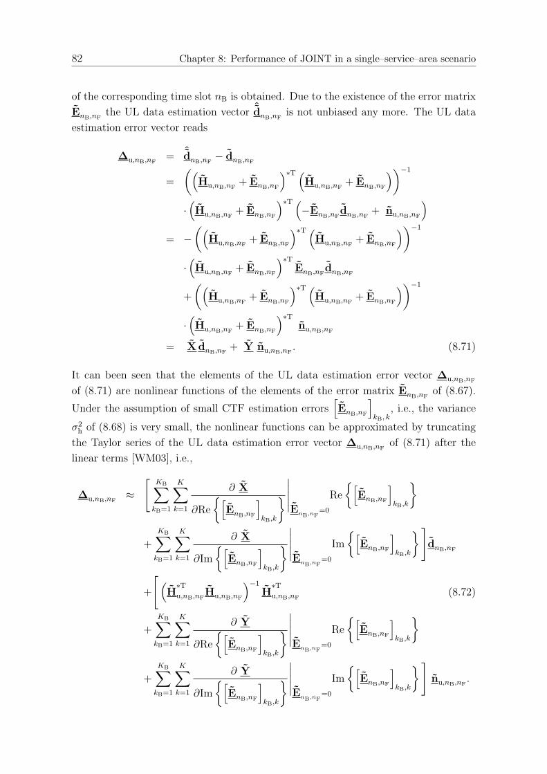
82 Chapter 8: Performance of JOINT in a single–service–area scenario
of the corresponding time slot nB is obtained. Due to the existence of the error matrix
EnB,nFthe UL data estimation vector ˆdnB,nF
is not unbiased any more. The UL data
estimation error vector reads
∆u,nB,nF= ˆdnB,nF
− dnB,nF
=
((Hu,nB,nF
+ EnB,nF
)∗T (Hu,nB,nF
+ EnB,nF
))−1
·(Hu,nB,nF
+ EnB,nF
)∗T (−EnB,nF
dnB,nF+ nu,nB,nF
)
= −((
Hu,nB,nF+ EnB,nF
)∗T (Hu,nB,nF
+ EnB,nF
))−1
·(Hu,nB,nF
+ EnB,nF
)∗TEnB,nF
dnB,nF
+
((Hu,nB,nF
+ EnB,nF
)∗T (Hu,nB,nF
+ EnB,nF
))−1
·(Hu,nB,nF
+ EnB,nF
)∗Tnu,nB,nF
= X dnB,nF+ Y nu,nB,nF
. (8.71)
It can been seen that the elements of the UL data estimation error vector ∆u,nB,nF
of (8.71) are nonlinear functions of the elements of the error matrix EnB,nFof (8.67).
Under the assumption of small CTF estimation errors[EnB,nF
]kB, k
, i.e., the variance
σ2h of (8.68) is very small, the nonlinear functions can be approximated by truncating
the Taylor series of the UL data estimation error vector ∆u,nB,nFof (8.71) after the
linear terms [WM03], i.e.,
∆u,nB,nF≈
[KB∑
kB=1
K∑
k=1
∂ X
∂Re
{[EnB,nF
]kB,k
}∣∣∣∣∣EnB,nF
=0
Re
{[EnB,nF
]kB,k
}
+
KB∑
kB=1
K∑
k=1
∂ X
∂Im
{[EnB,nF
]kB,k
}∣∣∣∣∣EnB,nF
=0
Im
{[EnB,nF
]kB,k
}]dnB,nF
+
[(H∗Tu,nB,nF
Hu,nB,nF
)−1
H∗Tu,nB,nF
(8.72)
+
KB∑
kB=1
K∑
k=1
∂ Y
∂Re
{[EnB,nF
]kB,k
}∣∣∣∣∣EnB,nF
=0
Re
{[EnB,nF
]kB,k
}
+
KB∑
kB=1
K∑
k=1
∂ Y
∂Im
{[EnB,nF
]kB,k
}∣∣∣∣∣EnB,nF
=0
Im
{[EnB,nF
]kB,k
}]nu,nB,nF
.

8.3 Impact of imperfect channel state information 83
After some simplifications we obtain from (8.72)
∆u,nB,nF≈ −
(H∗Tu,nB,nF
Hu,nB,nF
)−1
H∗Tu,nB,nF
EnB,nFdnB,nF
+(H∗Tu,nB,nF
Hu,nB,nF
)−1
H∗Tu,nB,nF
nu,nB,nF
+(H∗Tu,nB,nF
Hu,nB,nF
)−1
E∗Tu,nB,nF
nu,nB,nF
−(H∗Tu,nB,nF
Hu,nB,nF
)−1 (H∗Tu,nB,nF
Eu,nB,nF+ E
∗Tu,nB,nF
Hu,nB,nF
)
·(H∗Tu,nB,nF
Hu,nB,nF
)−1
H∗Tu,nB,nF
nu,nB,nF. (8.73)
With (8.10) and (8.11) the covariance matrix of the UL data estimation error vector
∆u,nB,nFof (8.71) reads
R∆u= E
{(ˆdnB,nF
− dnB,nF
)(ˆdnB,nF
− dnB,nF
)∗T}
≈ 2σ2(H∗Tu,nB,nF
Hu,nB,nF
)−1
+ 2Ed · 2σ2h ·K
(H∗Tu,nB,nF
Hu,nB,nF
)−1
+2σ2 · 2σ2htrace
{(H∗Tu,nB,nF
Hu,nB,nF
)−1} (
H∗Tu,nB,nF
Hu,nB,nF
)−1
+2σ2 · 2σ2h (KB −K)
(H∗Tu,nB,nF
Hu,nB,nF
)−2
= 2σ2(H∗Tu,nB,nF
Hu,nB,nF
)−1
·(
1 +2Ed · 2σ2
h ·K2σ2
+ 2σ2htrace
{(H∗Tu,nB,nF
Hu,nB,nF
)−1})
+2σ2h (KB −K)
(H∗Tu,nB,nF
Hu,nB,nF
)−2
. (8.74)
For the special full–loaded case that the number KB of APs per SA is equal to the
number K of MTs per SA, the last term 2σ2h (KB −K)
(H∗Tu,nB,nF
Hu,nB,nF
)−2
on the
right hand of (8.74) becomes zero so that (8.74) can be rewritten as
R∆u≈ 2σ2
(H∗Tu,nB,nF
Hu,nB,nF
)−1
·(
1 +2Ed · 2σ2
h ·K2σ2
+ 2σ2htrace
{(H∗Tu,nB,nF
Hu,nB,nF
)−1})
︸ ︷︷ ︸ξu,nF
, (8.75)
where ξu,nFis a factor greater than one. Consequently, with (8.18), (8.24) and (8.75)
the SNR
γ(k)u,nB,nF
=Ed
σ2 · ξu,nF
[(H∗Tu,nB,nF
Hu,nB,nF
)−1]
k,k
=γ
(k)u,nB,nF
ξu,nF
(8.76)

84 Chapter 8: Performance of JOINT in a single–service–area scenario
of the data symbol d(k)
u,nB,nFin the UL can be obtained in the case of imperfect CSI.
It can be seen that the CTF estimation error matrix EnB,nFof (8.67) acts like the
additional noise, which makes the system performance worse. If QPSK is applied, with
(8.76) the bit error probability of (8.25) can be rewritten as
P(k)b,u,nB,nF
=1
2erfc
√γ
(k)u,nB,nF
2
(8.77)
=1
2erfc
√√√√√√T
(k)u,nB,nF
σ2
2ξu,nF
[(H∗Tu,nB,nF
Hu,nB,nF
)−1]
k,k
.
8.3.2.3 Impact on the downlink data transmission
At the CU only the CTF estimation matrix ˆHu,nB,nFof (8.67) is available for the TxZF
JT of the DL. Therefore, the modulation matrix Md,nB,nFof (8.29) of the time slot nB
has to be constructed with the CTF estimation matrix ˆHu,nB,nFof (8.67), i.e.,
Md,nB,nF= ˆH
∗Td,nB,nF
(ˆHd,nB,nF
ˆH∗Td,nB,nF
)−1
= ˆH∗u,nB,nF
(ˆH
T
u,nB,nF
ˆH∗u,nB,nF
)−1
(8.78)
=(Hu,nB,nF
+ EnB,nF
)∗ ((Hu,nB,nF
+ EnB,nF
)T (Hu,nB,nF
+ EnB,nF
)∗)−1
.
It can be seen that the modulator matrix Md,nB,nFof (8.78) is a nonlinear function
of the error matrix EnB,nFof (8.67). Similarly as in the UL, with the assumption of
small CTF estimation errors[EnB,nF
]kB,k
, i.e., with a small variance σ2h of (8.68), the
modulator matrix Md,nB,nFof (8.78) can be approximated by a linear function of the
error matrix EnB,nFof (8.67) by truncating the Taylor series of Md,nB,nF
of (8.78) after

8.3 Impact of imperfect channel state information 85
the linear terms [WM03]. Therefore,
Md,nB,nF≈ H
∗u,nB,nF
(H
T
u,nB,nFH∗u,nB,nF
)−1
+
KB∑
kB=1
K∑
k=1
∂Md,nB,nF
∂Re
{[EnB,nF
]kB,k
}∣∣∣∣∣EnB,nF
=0
Re
{[EnB,nF
]kB,k
}
+
KB∑
kB=1
K∑
k=1
∂Md,nB,nF
∂Im
{[EnB,nF
]kB,k
}∣∣∣∣∣EnB,nF
=0
Im
{[EnB,nF
]kB,k
}
≈ H∗u,nB,nF
(H
T
u,nB,nFH∗u,nB,nF
)−1
+ E∗nB,nF
(H
T
u,nB,nFH∗u,nB,nF
)−1
−H∗u,nB,nF
(H
T
u,nB,nFH∗u,nB,nF
)−1
·(H
T
u,nB,nFE∗nB,nF
+ ET
nB,nFH∗u,nB,nF
)(H
T
u,nB,nFH∗u,nB,nF
)−1
(8.79)
can be obtained after some simplifications.
Consequently, with (8.7), (8.28) and (8.79) the DL data estimation vector
ˆdnB,nF= Hd,nB,nF
Md,nB,nFdnB,nF
+ nd,nB,nF
= HT
u,nB,nFMd,nB,nF
dnB,nF+ nd,nB,nF
(8.80)
can be obtained. With (8.80) the DL data estimation error vector reads
∆d,nB,nF= ˆdnB,nF
− dnB,nF
≈ E∗nB,nF
H∗u,nB,nF
(H
T
u,nB,nFH∗u,nB,nF
)−1
dnB,nF+ nd,nB,nF
. (8.81)
It can be seen that the unbiased estimation in the DL is destroyed by the CTF esti-
mation error matrix EnB,nFof (8.67), i.e., the DL data estimation error vector ∆d,nB,nF
consists of not only the noise part nd,nB,nFof (8.81), but contains also the interference
part, which is the first term on the right side of (8.81). With (8.10) and (8.11) the
covariance matrix
R∆d≈
(2σ2 + 2Ed · 2σ2
h · trace
{(H
T
u,nB,nFH∗u,nB,nF
)−1})
· IK (8.82)
of the DL data estimation error vector ∆d,nB,nFof (8.81) can be obtained.
The transmit energy T(k)d,nB,nF
of (8.30) invested for the data symbol d(k)
nB,nFin the DL is
also influenced by imperfect CSI. With (8.30) and (8.79) the transmit energy reads
T(k)d,nB,nF
= Ed
[M
∗Td,nB,nF
Md,nB,nF
]k,k
= Ed
[(H
T
u,nB,nFH∗u,nB,nF
)−1]
k,k
·(
1 + 2σ2h · trace
{(H
T
u,nB,nFH∗u,nB,nF
)−1})
+Ed · 2σ2h · (KB −K)
[(H
T
u,nB,nFH∗u,nB,nF
)−2]
k,k
. (8.83)

86 Chapter 8: Performance of JOINT in a single–service–area scenario
It can be seen that imperfect CSI leads to an increased transmit energy T(k)d,nB,nF
of
(8.83). In the full–loaded case of KB equal to K the last term on the right side of
(8.83) becomes zero. In such a case with (8.82) and (8.83) the SNR
γ(k)d,nB,nF
=Ed
σ2
(1 +
2Ed·2σ2h
2σ2 trace
{(H
T
u,nB,nFH∗u,nB,nF
)−1})
≈T
(k)d,nB,nF
σ2[(H
T
u,nB,nFH∗u,nB,nF
)−1]
k,k
· 1(1 +
2Ed·2σ2h
2σ2 trace
{(H
T
u,nB,nFH∗u,nB,nF
)−1})
· 1(1 + 2σ2
h · trace
{(H
T
u,nB,nFH∗u,nB,nF
)−1})
=
T(k)d,nB,nF
σ2
ξd,nF
[(H
T
u,nB,nFH∗u,nB,nF
)−1]
k,k
(8.84)
of the data symbol d(k)
d,nB,nFin the DL can be obtained, where
ξd,nF=
(1 +
2Ed · 2σ2h
2σ2trace
{(H
T
u,nB,nFH∗u,nB,nF
)−1})
= ·(
1 + 2σ2h · trace
{(H
T
u,nB,nFH∗u,nB,nF
)−1})
(8.85)
holds. It can be seen that the degradation factor ξd,nFof (8.85) is greater than one.
(8.84) shows that the worse system performance in the DL results from the interference,
see (8.82), and the increased transmit energy T(k)d,nB,nF
of (8.83) is due to the existence
of the CTF estimation error matrix EnB,nFof (8.67).
It is assumed that the QPSK modulation is applied. The bit error probability of (8.32)
can be rewritten as
P(k)b,d,nB,nF
=1
2erfc
√γ
(k)d,nB,nF
2
(8.86)
=1
2erfc
√√√√√√√
T(k)d,nB,nF
σ2
2ξd,nF
[(H
T
u,nB,nFH∗u,nB,nF
)−1]
k,k
.

8.4 Numerical results 87
8.4 Numerical results
8.4.1 Fixed channel snapshot
In order to visualize the analysis in the previous sections an exemplary single–SA
scenario with a fixed CTF matrix
Hu,nB,nF= H
T
d,nB,nF=
1 2 33 1 12 2 0
, (8.87)
with
KB = K = 3, (8.88)
is considered in the present subsection. K equal to 3 data symbols d(k)
u,nB,nFand d
(k)
d,nB,nF
are transmitted in the UL and in the DL, which result in the individual bit error
probabilities P(k)b,u,nB,nF
in the UL and the bit error probabilities P(k)b,d,nB,nF
in the DL,
respectively. For the sake of simplicity and clarity, in the following the bit error prob-
abilities P(1)b,u,nB,nF
and P(1)b,d,nB,nF
of the data symbols d(1)
u,nB,nFand d
(1)
d,nB,nFare depicted.
Firstly, as depicted in Fig. 8.3, the fact that the simulation results with perfect CSI
match the theoretical results perfectly illustrates the duality of the UL and the DL
performances of JOINT in the case that perfect CSI is available.
Secondly, it is assumed that only the noise plays a role in causing the CTF estima-
tion error EnB,nFof (8.67). Therefore, with (8.51) the variance σ2
h of (8.68) is only
proportional to the variance σ2 of the noise, i.e.,
σ2h = σ2
h,n ∝ σ2. (8.89)
In such a case with (8.77) and (8.86) the equality
P(1)b,u,nB,nF
= P(1)b,d,nB,nF
(8.90)
still holds. As depicted in Fig. 8.3 the simulation results match the theoretical results
obtained by (8.77) and (8.86) well. This means that the analysis based on the Taylor
series (8.77) and (8.86) are good approximations. The bit error probability curves in
such cases are shifted versions of the MF bound, and parallel to the curves of the case
with perfect CSI. This shows that the CTF estimation error matrix EnB,nFof (8.67)
caused by the noise only acts like additional noise.
Finally, it is assumed that only the time variance of channels is to be considered to
cause the CTF estimation error matrix EnB,nFof (8.67). In such a case the variance
σ2h = σ2
h,tv (8.91)

88 Chapter 8: Performance of JOINT in a single–service–area scenario
of (8.68) only depends on the time–variant channels according to (8.63). For the fixed
channel snapshot of (8.87), the fixed value σ2h equal to 0.09 is simply assumed for the
variance σ2h of (8.91), which corresponds to large errors since the standard deviation
σh equal to 0.3 is rather high. Due to the fixed variance σ2h, which is independent of
the variance σ2 of the noise, the equality of (8.90) does not hold any more. As the
ratio T(k)u,nB,nF/σ2 increases to very large values, the bit error probability P
(k)b,u,nF
of (8.77)
converges to
P(k)b,u,∞,nB,nF
= limT
(k)u,nB,nF
σ2 →∞P
(k)b,u,nB,nF
≈ 1
2erfc
√√√√√1
4σ2h ·K
[(H∗Tu,nB,nF
Hu,nB,nF
)−1]
k,k
. (8.92)
Similarly, as the ratio T(k)d,nB,nF
/σ2 increases to very large values, the bit error probability
P(k)b,d,nB,nF
of (8.86) converges to
P(k)b,d,∞,nB,nF
= limT
(k)d,nB,nF
σ2 →∞
P(k)b,d,nB,nF
≈ 1
2erfc
√√√√√1
4σ2h · trace
{(H∗Tu,nB,nF
Hu,nB,nF
)−1}
. (8.93)
According to (8.92) and (8.93) the bit error probability curves of the UL and of the DL
converge to different error floors. This means as well, that (8.90) cannot be satisfied
any more for the fixed σ2h of the CTF error EnB,nF
of (8.67). In other words, imperfect
CSI caused by the time–variant channels leads to different error floors of the bit error
probability curves in the UL and in the DL. In Fig. 8.4 the mentioned phenomenon can
be seen.
8.4.2 Rayleigh fading channel
The influence of imperfect CSI on the individual bit error probabilities P(1)b,u,nB,nF
of
(8.77) in the UL and the bit error probabilities P(1)b,d,nB,nF
of (8.86) in the DL with a
snapshot of the CTF matrix Hu,nB,nFof (8.87) has been analyzed in detail. In the
present subsection the average bit error probability performance in a scenario with
living Rayleigh fading channels is focused.

8.4 Numerical results 89
−10 −5 0 5 10 15 2010
−3
10−2
10−1
100
UL simulation results
MF bound
with imperfect CSI
with perfect CSI
DL simulation results
theoretical results
P(1)
b,n
B,n
F
10 log10
(
T(1)nB,nF
σ2
)
/ dB
Fig. 8.3. Individual bit error probability P(1)b,nB,nF
, if only the
noise plays a role in the CTF estimation error EnB,nF,
Ep/Ed = 1
JCE is applied in the simulations. Both factors, the noise and the time variance
of the channels, are taken into account. In order to achieve different degrees of the
time variance, different maximum velocities vmax of the MTs are assumed. In the
simulations, the OFDM frame is assumed to consist of NBU equal to five slots for the
UL transmission, NBP equal to one slot for the UL pilot transmission and NBD equal
to five slots for the DL transmission. For the other simulation parameters, refer to
Table. 3.1.
The average bit error probability Pb is obtained by averaging over the fast fading
channels, the multiple slots in the UL or in the DL, and the corresponding MTs. T
represents the average transmit energy of the data symbols d(k)
u,nFfor the UL or d
(k)
d,nF
for the DL. As depicted in Fig. 8.5, the Pb curves of the UL cases are plotted with
solid lines, and the Pb curves of the DL cases are plotted with marks. The following
conclusions can be drawn from these curves:
• The Pb curves in the UL and in the DL are almost the same for the cases with
perfect CSI or imperfect CSI.

90 Chapter 8: Performance of JOINT in a single–service–area scenario
−10 −5 0 5 10 15 2010
−3
10−2
10−1
100
with perfect CSI
in the UL
with imperfect CSI
simulation results in the DL
theoretical results
MF bound
P(1)
b,n
B,n
F
10 log10
(
T(1)nB,nF
σ2
)
/ dB
Fig. 8.4. Individual bit error probability P(1)b,nB,nF
, if only timevariance of channels plays a role in the CTF estimationerror EnB,nF
• The noise and the time variance of the channels play a joint role in influencing
the JCE performance and the Pb performance. For instance, when the noise
vanishes, the time variance of channels dominates. Therefore, the Pb curves of
the cases with imperfect CSI converge to the error floors finally.
• The value of the maximum velocity vmax significantly influences the error floors
in the cases with imperfect CSI. Different maximum velocities vmax correspond
to different degrees of the time variance. The greater the maximum velocity vmax
is, the more significant the time variance of channels appears, and the worse
performance becomes, for the fixed frame structure. Therefore, if the MTs move
very fast, it should be considered to adjust the frame structure and to process
JCE more frequently in order to track the time–variant channels accurately.

8.4 Numerical results 91
−10 −5 0 5 10 15 2010
−3
10−2
10−1
100
marks: DL
UL & DL with JCE
UL & DL with perfect CSI
lines: UL
= 0, 50, 100 km/h
Pb
10 log10
(
T
σ2
)
/ dB
vmax
Fig. 8.5. Average bit error probability Pb, with the Raleigh fadingchannel, KB = K = 2, NBU = NBD = 5, ∆t = 32µs,NF = 512, Ep/Ed = 1

92
Chapter 9
Performance of JOINT in amultiple–service–area scenario
9.1 Preliminary remarks
In Chapter 8 the system performance of JOINT, especially in the single–SA scenario,
in which the inter–SA MAI is provisionally not taken into consideration, has been in-
vestigated. In reality mobile radio systems are usually interference–limited. Therefore,
it is necessary to investigate the performance of JOINT in a multiple–SA scenario,
in which not only the noise but also the MAI, including the intra–SA MAI and the
inter–SA MAI, are taken into account [LWZ04].
In the present chapter, first the multiple–SA scenario is described. Then the system
performance, in terms of the average BERs and the BER statistics, are analyzed based
on simulation results carried out with the JOINT simulation chain described in Chapter
7. Moreover, according to some given system criterion the spectrum efficiency of JOINT
is studied.
It is assumed that the perfect SA–specific CSI data are available at the corresponding
CU for the UL and the DL in the simulations. Since great amounts of simulations
have to be carried out, the computational effort is a critical problem. Thanks to the
application of OFDM the subcarrierwise processing is possible, see Section 3.2. In the
present chapter only an arbitrary subcarrier is considered without loss of generality.
9.2 Multiple–service–area scenario
In order to investigate the advantages of JOINT over conventional cellular systems in
the interference elimination, it is necessary to define a multiple–SA scenario, which is
comparable to the cellular scenario [LWZ04].
In contrast to cellular systems, the basic entity of JOINT is the SA, consisting of
several neighboring sub–areas, which are equivalent to cells in cellular systems. For
the sake of simplicity, it is assumed that there is one AP located at the center of each
sub–area, and there is at most one active MT randomly distributed in each sub–area.

9.2 Multiple–service–area scenario 93
� � � � � �� � � � � �� � � � � �� � � � � �� � � � � �� � � � � �� � � � � �
� � � � � �� � � � � �� � � � � �� � � � � �� � � � � �� � � � � �� � � � � �
� � � � � � �� � � � � � �� � � � � � �� � � � � � �� � � � � � �� � � � � � �� � � � � � �
� � � � � � �� � � � � � �� � � � � � �� � � � � � �� � � � � � �� � � � � � �� � � � � � �
� � � � � � �� � � � � � �� � � � � � �� � � � � � �� � � � � � �� � � � � � �� � � � � � �
� � � � � �� � � � � �� � � � � �� � � � � �� � � � � �� � � � � �� � � � � �
� � � � � � �� � � � � � �� � � � � � �� � � � � � �� � � � � � �� � � � � � �� � � � � � �
� � � � � �� � � � � �� � � � � �� � � � � �� � � � � �� � � � � �� � � � � �
� � � � � � �� � � � � � �� � � � � � �� � � � � � �� � � � � � �� � � � � � �� � � � � � �
� � � � � �� � � � � �� � � � � �� � � � � �� � � � � �� � � � � �� � � � � �
� � � � � � �� � � � � � �� � � � � � �� � � � � � �� � � � � � �� � � � � � �� � � � � � �
� � � � � �� � � � � �� � � � � �� � � � � �� � � � � �� � � � � �� � � � � �
� � � � � �� � � � � �� � � � � �� � � � � �� � � � � �� � � � � �� � � � � �
� � � � � � �� � � � � � �� � � � � � �� � � � � � �� � � � � � �� � � � � � �� � � � � � �
� � � � � � �� � � � � � �� � � � � � �� � � � � � �� � � � � � �� � � � � � �� � � � � � �
� � � � � � �� � � � � � �� � � � � � �� � � � � � �� � � � � � �� � � � � � �� � � � � � �
� � � � � �� � � � � �� � � � � �� � � � � �� � � � � �� � � � � �� � � � � �
π
3
R
Fig. 9.1. An example of the SA based system architecture withthe SA size KB = 3 and the reuse factor r = 3
As depicted in Fig. 9.1, the hexagons represent the sub–areas with radius R, and the
APs and the MTs are located in the corresponding hexagonal sub–areas. The radius
R = 250 m (9.1)
of the hexagonal sub–area is assumed in the following investigations.
The number KB of APs per SA also represents the SA size, indicating how many
sub–areas there are per SA. A SA is a cluster of neighboring sub–areas, which share
the same frequency resource. Neighboring SAs, which form a cluster of SAs, may use
different frequency resources, i.e., the frequency resources can be reused among the
different clusters of SAs. The size of the cluster of SAs is described by the reuse factor
r. Fig. 9.1 depicts an excerpt of the area, which is covered by the multiple SAs. The
neighboring hexagonal sub–areas with the same pattern form a SA using the same
frequency resource. The neighboring SAs with different patterns form a cluster of SAs
using different frequency resources. The SAs with the same pattern represent the co–
channel SAs, in which we are interested. In the case of KB equal to one, i.e., each SA
comprising only a single sub–area, the SA–based system architecture is equivalent to
the cellular system.
Due to the hexagonal shape of the sub–areas, in most cases the SAs are non–hexagonal,
except for the SA size KB equal to one. Because of different combinations of the SA
size KB and the reuse factor r, it is difficult to define a scenario with fixed dimensions,
in which the SA based system architectures are applied. Fortunately, it is found that,
whatever the SAs look like, if one of the APs in one SA is chosen as the reference
AP, the reference APs of the neighboring four co–channel SAs always form a diamond,

94 Chapter 9: Performance of JOINT in a multiple–service–area scenario
� � � � �� � � � �� � � � �� � � � �
� � � � �� � � � �� � � � �� � � � �
� � � �� � � �� � � �� � � �
� � � �� � � �� � � �� � � �� � � �
� � � �� � � �� � � �
� � � �� � � �� � � �� � � �
� � � � �� � � � �� � � � �� � � � �
� � � �� � � �� � � �� � � �
� � � �� � � �� � � �� � � �
� � � �� � � �� � � �� � � �
� � � � �� � � � �� � � � �� � � � �
� � � �� � � �� � � �� � � �
� � � �� � � �� � � �� � � �� � � �
� � � �� � � �� � � �
� � � �� � � �� � � �� � � �
� � � � �� � � � �� � � � �� � � � �
� � � � �� � � � �� � � � �� � � � �
� � � �� � � �� � � �� � � �
� � � �� � � �� � � �� � � �� � � �
� � � �� � � �� � � �
� � � �� � � �� � � �� � � �
� � � � �� � � � �� � � � �� � � � �
� � � �� � � �� � � �� � � �
� � � �� � � �� � � �� � � �
� � � �� � � �� � � �� � � �� � � �
� � � �� � � �� � � �
� � � �� � � �� � � �� � � �
number of co−channel SAs
reference cluster of SAs
NSA = 5 × 5
Fig. 9.2. Considered area with the SA size KB = 3 and the reusefactor r = 3
as depicted in Fig. 9.1. In other words, the reference APs of the co–channel SAs are
located along a parallelogram grid. In the following simulations, instead of a scenario
with fixed dimensions, the quasi–parallelogram scenario with the fixed number NSA of
the co–channel SAs, e.g.,
NSA = 5× 5, (9.2)
are investigated. As shown in Fig. 9.2, the reference cluster of SAs is at the center of the
given scenario. Most co–channel interfering SAs, which have the dominant influence
on the reference SA are included so that with a finite scenario we can approximate the
ideal infinite scenario.
The random channel with Rayleigh fading and log–normal fading described in Subsec-
tion 2.3.2 is assumed in the investigation. Concerning the slow fading, the dual–slope
model [XBMLS92] is applied. For the corresponding channel parameters, refer to Table
3.1 in Section 3.4.
In the multiple–SA scenario described above, the distances between the MTs and APs
play a role to determine the CTFs between the MTs and the APs since slow fading
is taken into account. Therefore, the positions of the APs and the MTs are critical
concerning the scenario realizations. Unlike conventional cellular systems, the challenge
of implementation of such a multiple–SA scenario lies in locating the APs and the MTs
based on the SA concept. For the details on the positions of the APs and the MTs,
refer to Appendix A.

9.3 Modified system model 95
9.3 Modified system model
9.3.1 Uplink system model in a multiple–service–area sce-nario
The UL and DL system models introduced in Sections 5.2 and 6.2 have to be extended
to adapt to the multiple–SA scenario [LWZ04]. On the considered subcarrier nF, the
total UL data vector of dimension KNSA reads
du,mul,nF=
(d
(1)
u,nF
T
. . . d(NSA)
u,nF
T)T
=(d
(1)
u,nF. . . d
(K)
u,nF. . . d
((NSA−1)K+1)
u,nF. . . d
((NSA−1)K+K)
u,nF
)T
. (9.3)
The total UL CTF matrix
Hu,mul,nF=
H(1,1)
nF· · · H
(NSA,1)
nF...
...
H(1,NSA)
nF· · · H
(NSA,NSA)
nF
(9.4)
of the whole scenario consists of NSA ×NSA submatrices
H(nSA,n′SA)
nF=
h((nSA−1)K+1,(n′SA−1)KB+1)
nF· · · h
((nSA−1)K+K,(n′SA−1)KB+1)
nF...
...
h((nSA−1)K+1,(n′SA−1)KB+KB)
nF· · · h
((nSA−1)K+K,(n′SA−1)KB+KB)
nF
, (9.5)
each of dimensions KB ×K including the CTFs between the K MTs in the SA nSA,
nSA = 1 . . . NSA, and the KB APs in the SA n′SA, n′SA = 1 . . . NSA. With (9.4) and the
total UL noise vector
nu,mul,nF=
(n(1)
u,nF
T. . . n(NSA)
u,nF
T)T
=(n(1)
u,nF. . . n(KB)
u,nF. . . n((NSA−1)KB+1)
u,nF. . . n((NSA−1)KB+KB)
u,nF
)T(9.6)
of dimension KBNSA the total UL receive vector
eu,mul,nF=
(e(1)
u,nF
T. . . e(NSA)
u,nF
T)T
=(e(1)u,nF
. . . e(KB)u,nF
. . . e((NSA−1)KB+1)u,nF
. . . e((NSA−1)KB+KB)u,nF
)T(9.7)
of dimension KBNSA becomes
eu,mul,nF= Hu,mul,nF
du,mul,nF+ nu,mul,nF
(9.8)

96 Chapter 9: Performance of JOINT in a multiple–service–area scenario
according to (3.17) and (5.4). Concerning the SA nSA, with the application of the
linear RxZF JD [Kle96, Skl04] the SA–specific data estimate vector ˆd(nSA)
u,nFof (5.11)
can be rewritten as [LWZ04]
ˆd(nSA)
u,nF=
(H
(nSA,nSA)
nF
∗TH
(nSA,nSA)
nF
)−1
H(nSA,nSA)
nF
∗Te(nSA)
u,nF
= d(nSA)
u,nF+
(H
(nSA,nSA)
nF
∗TH
(nSA,nSA)
nF
)−1
H(nSA,nSA)
nF
∗T ∑
n′SA 6=nSA
H(n′SA,nSA)
u,nFd
(n′SA)
nF
︸ ︷︷ ︸inter−SA MAI
+
(H
(nSA,nSA)
nF
∗TH
(nSA,nSA)
nF
)−1
H(nSA,nSA)
nF
∗Tn(nSA)
nF
︸ ︷︷ ︸enhanced noise
. (9.9)
It can be seen that the data estimate vector ˆd(nSA)
u,nFof (9.9) is not unbiased any
more, since the RxZF detector matrix
(H
(nSA,nSA)
nF
∗TH
(nSA,nSA)
nF
)−1
H(nSA,nSA)
nF
∗Tof
(9.9), which is designed for the SA nSA, cannot counteract the interfering sig-
nals∑
n′SA 6=nSAH
(n′SA,nSA)
u,nFd
(n′SA)
nFof (9.9) from the other co–channel SAs n′SA. Both
the inter–SA MAI
(H
(nSA,nSA)
nF
∗TH
(nSA,nSA)
nF
)−1
H(nSA,nSA)
nF
∗T ∑n′SA 6=nSA
H(n′SA,nSA)
u,nFd
(n′SA)
nF
of (9.9) and the enhanced noise
(H
(nSA,nSA)
nF
∗TH
(nSA,nSA)
nF
)−1
H(nSA,nSA)
nF
∗Tn(nSA)
nFof (9.9)
account for the UL data estimation error vector [LWZ04]
ˆd(nSA)
u,nF− d
(nSA)
u,nF=
(H
(nSA,nSA)
nF
∗TH
(nSA,nSA)
nF
)−1
H(nSA,nSA)
nF
∗T ∑
n′SA 6=nSA
H(n′SA,nSA)
u,nFd
(n′SA)
nF
︸ ︷︷ ︸inter−SA MAI
+
(H
(nSA,nSA)
nF
∗TH
(nSA,nSA)
nF
)−1
H(nSA,nSA)
nF
∗Tn(nSA)
nF
︸ ︷︷ ︸enhanced noise
(9.10)
in the corresponding SA nSA.
9.3.2 Downlink system model in a multiple–service–area sce-nario
On the subcarrier nF, the total DL data vector of dimension KNSA reads
dd,mul,nF=
(d
(1)
d,nF
T
. . . d(NSA)
d,nF
T)T
=(d
(1)
d,nF. . . d
(K)
d,nF. . . d
((NSA−1)K+1)
d,nF. . . d
((NSA−1)K+K)
d,nF
)T
. (9.11)

9.3 Modified system model 97
Concerning the SA nSA, with the application of the linear TxZF JT [MBW+00,
TWMB01, Skl04], the SA–specific DL transmit vector of (6.2) reads
s(nSA)d,nF
= H(nSA,nSA)
nF
∗ (H
(nSA,nSA)
nF
T
H(nSA,nSA)
nF
∗)−1
︸ ︷︷ ︸M
(nSA)
TxZF,nF
d(nSA)
d,nF. (9.12)
With the total UL CDF matrix Hu,mul,nFof (9.4), with the total DL transmit vector
sd,mul,nF=
(s(1)d,nF
T. . . s
(NSA)d,nF
T)T
(9.13)
of dimension KBNSA consisting of NSA SA–specific transmit vector s(nSA)d,nF
of (9.13) and
with the total DL noise vector
nd,mul,nF=
(n
(1)d,nF
T. . . n
(NSA)d,nF
T)T
=(n
(1)d,nF
. . . n(K)d,nF
. . . n((NSA−1)K+1)d,nF
. . . n((NSA−1)K+K)d,nF
)T
(9.14)
of dimension KNSA the total DL receive vector
ed,mul,nF=
(e
(1)d,nF
T. . . e
(NSA)d,nF
T)T
=(e(1)d,nF
. . . e(K)d,nF
. . . e((NSA−1)K+1)d,nF
. . . e((NSA−1)K+K)d,nF
)T
(9.15)
of dimension KNSA is constructed as
ed,mul,nF= H
T
u,mul,nFsd,mul,nF
+ nd,mul,nF. (9.16)
Consequently, the SA–specific data estimate vector
ˆd(nSA)
d,nF= e
(nSA)d,nF
= d(nSA)
d,nF+ n
(nSA)d,nF
(9.17)
+∑
n′SA 6=nSA
H(nSA,n′SA)
nF
T
H(n′SA,n′SA)
nF
∗ (H
(n′SA,n′SA)
nF
T
H(n′SA,n′SA)
nF
∗)−1
d(n′SA)
d,nF
︸ ︷︷ ︸inter−SA MAI
of the SA–specific data vector d(nSA)
d,nFof (9.11) is obtained.
It can be seen that the SA–specific data estimate vector ˆd(nSA)
d,nF
of (9.17) is not unbiased any more due to the inter–SA MAI∑
n′SA 6=nSAH
(nSA,n′SA)
nF
T
H(n′SA,n′SA)
nF
∗ (H
(n′SA,n′SA)
nF
T
H(n′SA,n′SA)
nF
∗)−1
d(n′SA)
d,nFof (9.17)

98 Chapter 9: Performance of JOINT in a multiple–service–area scenario
coming from the other co–channel SAs n′SA. The inter–SA MAI∑
n′SA 6=nSAH
(nSA,n′SA)
nF
T
H(n′SA,n′SA)
nF
∗ (H
(n′SA,n′SA)
nF
T
H(n′SA,n′SA)
nF
∗)−1
d(n′SA)
d,nFof (9.17) and
the noise n(nSA)d,nF
of (9.17) account for the DL data estimation error vector
ˆd(nSA)
d,nF− d
(nSA)
d,nF= n
(nSA)d,nF
(9.18)
+∑
n′SA 6=nSA
H(nSA,n′SA)
nF
T
H(n′SA,n′SA)
nF
∗ (H
(n′SA,n′SA)
nF
T
H(n′SA,n′SA)
nF
∗)−1
d(n′SA)
d,nF
︸ ︷︷ ︸inter−SA MAI
in the corresponding SA nSA.
9.4 Average bit error rate
In the system where the noise and the MAI are considered, the average BERs Pb
versus the pseudo SNR, i.e., the ratio T/σ2 of the average transmit energy T of the
data symbols d(k)
u,nFor d
(k)
d,nFto the variance σ2 of the noise reveal the performance,
especially from the viewpoint of the energy transmission, as discussed in Subsection
8.2.2. Thermal noise is assumed at the receiver. Described by the noise figure F
[Cou97], which is an inherent property of the receiver device, the noise variance σ2 of
(4.12), (5.6) and (6.7), reads [Cou97]
σ2 = κT0 B F, (9.19)
where κ is Boltzmann’s constant equal to 1.38× 10⁻²³ J/K, T0 is the absolute temper-
ature, e.g., equal to 290 K, and the bandwidth B of the considered system is equal to
the subcarrier spacing ∆fnFof Table 3.1, since only a single subcarrier is considered
in the following investigation. With (9.19) the logarithmic ratio
10 log10
(T
σ2
)= 10 log10
(T
10−3 w
)− 10 log10 F + 10 log10
(10−3 w
κT0 B
)
= TdBm − FdB + const (9.20)
depends only on the difference between the logarithmic average transmit energy TdBm
in dBm and the logarithmic noise figure FdB in dB. The average BERs Pb are averaged
over all the individual BERs Pb in the UL and in the DL, respectively, in the reference
SA, which is the considered SA in the central cluster of SAs, as depicted in Fig. 9.2.
In the present section the simulation results are plotted as the curves of the average
BERs Pb versus the difference TdBm/dBm − FdB/dB. In the real system with a limit
of total transmit power 30 dBm [Cou97], the typical values
TdBm = 30 dBm− 10 log10 NF = 30 dBm− 10 log10 512 = 3 dBm (9.21)

9.4 Average bit error rate 99
and
FdB = 5 dB (9.22)
are usually valid.
Fig. 9.3 depicts the average BER performances of the equivalent cellular system, i.e.,
of the cases of
KB = K = 1, (9.23)
for different reuse factors r in the UL and in the DL, respectively. The average BER Pb
curves in the UL are plotted with solid lines, and the Pb curves in the DL are plotted
with marks. It is seen that the average Pb curves perform almost the same in the
UL and in the DL for the different reuse factors r = 1, 3, 4, 7, respectively. It proves
that the prices paid for the interference elimination with the application of linear ZF
[Kle96, Skl04] are the same in the UL and in the DL. This phenomenon is consistent
with the conclusion drawn in Section 8.2 concerning the duality of the UL and the DL
with perfect CSI.
−50 −40 −30 −20 −10 0 10 20 3010
−3
10−2
10−1
100
� � � � � � � � � � � � � � � � � � � � �� � � � � � � � � � � � � � � � � � � � �� � � � � � � � � � � � � � � � � � � � �
� � � � � � � � � � � � � � � � � � � � �� � � � � � � � � � � � � � � � � � � � �� � � � � � � � � � � � � � � � � � � � �
marks: DL
lines: UL
60 −50 −40 −30 −20 −10 0 10 20
TdBm/dBm − FdB/dB
Pb
r = 1, 3, 4, 7
Fig. 9.3. Average BERs Pb in the reference SA, KB = K = 1
Figs. 9.3 to 9.6 depict the average BER performances of JOINT with different com-
binations of the number K of MTs per SA, the number KB of APs per SA and the
reuse factor r, in the UL and in the DL, respectively. The Pb curves of the equivalent
cellular system for the corresponding reuse factors r are plotted with dashed lines as
references. The following can be stated:
• The Pb curves converge to error floors [LWZ04]. Since either the RxZF JD
[Kle96, Skl04] or the TxZF JT [MBL+00, TWMB01, Skl04] at the CU is applied

100 Chapter 9: Performance of JOINT in a multiple–service–area scenario
60 −50 −40 −30 −20 −10 0 10 20−50 −40 −30 −20 −10 0 10 20 3010
−3
10−2
10−1
100
−50 −40 −30 −20 −10 0 10 20 3010
−3
10−2
10−1
100
−50 −40 −30 −20 −10 0 10 20 3010
−3
10−2
10−1
100
−50 −40 −30 −20 −10 0 10 20 3010
−3
10−2
10−1
100
cellular system
cellular system
cellular system
60 −50 −40 −30 −20 −10 0 10 20 60 −50 −40 −30 −20 −10 0 10 20
60 −50 −40 −30 −20 −10 0 10 20 60 −50 −40 −30 −20 −10 0 10 20
cellular system
TdBm/dBm − FdB/dB
Pb
TdBm/dBm − FdB/dB
Pb K = 1, 2, 3
Pb
Pb
TdBm/dBm − FdB/dBTdBm/dBm − FdB/dB
K = 1, 2, 3
K = 1, 2, 3K = 1, 2, 3
r = 1 r = 3
r = 4 r = 7
Fig. 9.4. Average BERs Pb in the reference SA in the UL, KB = 3
based on the knowledge of the CTF matrix H(nSA,nSA)
nFof (9.5) of the correspond-
ing SA nSA regardless of the other co–channel SAs n′SA, the intra–SA MAI is
eliminated, while the inter–SA MAI in the multiple–SA scenario remains as a
factor degrading the UL or the DL performance, as well as the noise. Meanwhile,
the impact of the inter–SA MAI on the average BER performance, which greatly
depends on the average transmit energy TdBm of (9.20) for the given channel
model described in Subsection 2.3.2, does not change as the noise varies. There-
fore, when the logarithmic noise figure FdB of (9.20) is very small or the average
transmit energy TdBm of (9.20) is very large, i.e., TdBm of (9.20) dominates the
difference TdBm/dBm − FdB/dB of (9.20), the error floors occur, in the UL and
in the DL, respectively.
• It becomes obvious from Figs. 9.4 to 9.6 that as the increase of the number K
of MTs per SA the UL performance becomes worse due to the enlarged inter–
SA MAI and the extra enhanced noise to eliminate the increased intra–SA MAI

9.4 Average bit error rate 101
−50 −40 −30 −20 −10 0 10 20 3010
−3
10−2
10−1
100
−50 −40 −30 −20 −10 0 10 20 3010
−3
10−2
10−1
100
−50 −40 −30 −20 −10 0 10 20 3010
−3
10−2
10−1
100
−50 −40 −30 −20 −10 0 10 20 3010
−3
10−2
10−1
100
� � � � � � � � � � � � � � � � � � � � � �� � � � � � � � � � � � � � � � � � � � � �� � � � � � � � � � � � � � � � � � � � � �� � � � � � � � � � � � � � � � � � � � � �� � � � � � � � � � � � � � � � � � � � � �� � � � � � � � � � � � � � � � � � � � � �
� � � � � � � � � � � � � � � � � � � � � �� � � � � � � � � � � � � � � � � � � � � �� � � � � � � � � � � � � � � � � � � � � �� � � � � � � � � � � � � � � � � � � � � �� � � � � � � � � � � � � � � � � � � � � �� � � � � � � � � � � � � � � � � � � � � �
� � � � � � � � � � � � � � � � � � � � � �� � � � � � � � � � � � � � � � � � � � � �� � � � � � � � � � � � � � � � � � � � � �� � � � � � � � � � � � � � � � � � � � � � � � � � � � � � � � � � � � � � � � � � � �� � � � � � � � � � � � � � � � � � � � � �
� � � � � � � � � � � � � � � � � � � � � �� � � � � � � � � � � � � � � � � � � � � �
cellular system
cellular system
cellular system
60 −50 −40 −30 −20 −10 0 10 20 60 −50 −40 −30 −20 −10 0 10 20
60 −50 −40 −30 −20 −10 0 10 20 60 −50 −40 −30 −20 −10 0 10 20
cellular system
TdBm/dBm − FdB/dB
Pb
TdBm/dBm − FdB/dB
Pb
Pb
Pb
TdBm/dBm − FdB/dBTdBm/dBm − FdB/dB
K = 1, 2, 3, 4
K = 1, 2, 3, 4
K = 1, 2, 3, 4K = 1, 2, 3, 4
r = 1 r = 3
r = 4 r = 7
Fig. 9.5. Average BERs Pb in the reference SA in the UL, KB = 4
[LWZ04] according to (9.9). The DL performance is degraded as well due to the
enlarged inter–SA MAI according to (9.17).
• As the increase of the reuse factor r, the average distances between the interferers
of the co–channel SAs and the receivers in the reference SA correspondingly
increase so that the received inter–SA MAI decreases as well. Consequently the
system performance is greatly improved.
• It can bee seen in Figs. 9.4 to 9.6 that for the same number K of MTs per SA
and the same reuse factor r, a larger SA size KB corresponds to a better average
BER performance in the UL [LWZ04] as well as in the DL.
• Through the performance comparison of the case of full load, i.e., K equal KB, of
JOINT and the cellular system, whose simulation results are plotted with dashed
curves in Figs. 9.4 to 9.6, it is found that with the small–value reuse factor, e.g.,
r equal to one, the differences between the SA based system performances and
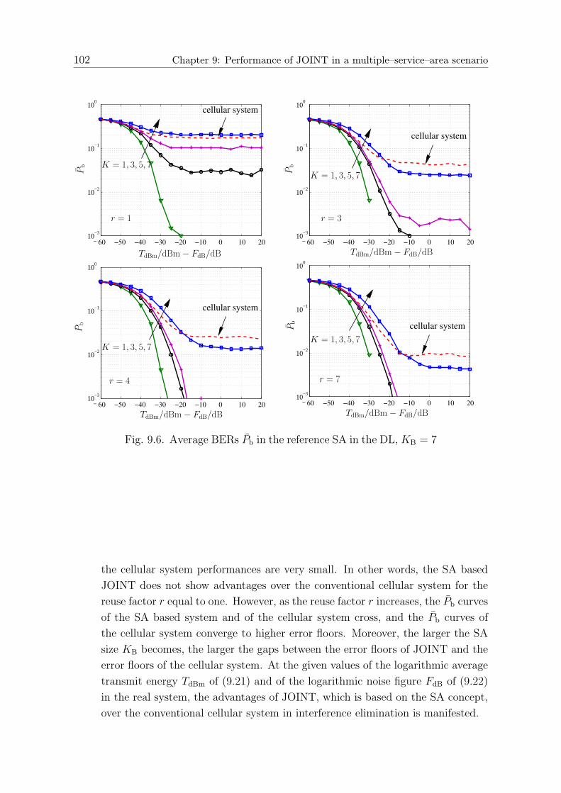
102 Chapter 9: Performance of JOINT in a multiple–service–area scenario
−50 −40 −30 −20 −10 0 10 20 3010
−3
10−2
10−1
100
−50 −40 −30 −20 −10 0 10 20 3010
−3
10−2
10−1
100
−50 −40 −30 −20 −10 0 10 20 3010
−3
10−2
10−1
100
−50 −40 −30 −20 −10 0 10 20 3010
−3
10−2
10−1
100
� � � � � � � � � � � � � � � � � � � � � �� � � � � � � � � � � � � � � � � � � � � �� � � � � � � � � � � � � � � � � � � � � �
� � � � � � � � � � � � � � � � � � � � � �� � � � � � � � � � � � � � � � � � � � � �� � � � � � � � � � � � � � � � � � � � � �
� � � � � � � � � � � � � � � � � � � � � �� � � � � � � � � � � � � � � � � � � � � �� � � � � � � � � � � � � � � � � � � � � �
� � � � � � � � � � � � � � � � � � � � � �� � � � � � � � � � � � � � � � � � � � � �� � � � � � � � � � � � � � � � � � � � � �
� � � � � � � � � � � � � � � � � � � � � �� � � � � � � � � � � � � � � � � � � � � �� � � � � � � � � � � � � � � � � � � � � �� � � � � � � � � � � � � � � � � � � � � �
� � � � � � � � � � � � � � � � � � � � � �� � � � � � � � � � � � � � � � � � � � � �� � � � � � � � � � � � � � � � � � � � � �
� � � � � � � � � � � � � � � � � � � � � �� � � � � � � � � � � � � � � � � � � � � �� � � � � � � � � � � � � � � � � � � � � �
cellular system
cellular system
60 −50 −40 −30 −20 −10 0 10 20 60 −50 −40 −30 −20 −10 0 10 20
60 −50 −40 −30 −20 −10 0 10 20 60 −50 −40 −30 −20 −10 0 10 20
cellular system
cellular system
TdBm/dBm − FdB/dB
Pb
TdBm/dBm − FdB/dB
Pb
Pb
Pb
TdBm/dBm − FdB/dBTdBm/dBm − FdB/dB
K = 1, 3, 5, 7
K = 1, 3, 5, 7
K = 1, 3, 5, 7K = 1, 3, 5, 7
r = 1 r = 3
r = 4 r = 7
Fig. 9.6. Average BERs Pb in the reference SA in the DL, KB = 7
the cellular system performances are very small. In other words, the SA based
JOINT does not show advantages over the conventional cellular system for the
reuse factor r equal to one. However, as the reuse factor r increases, the Pb curves
of the SA based system and of the cellular system cross, and the Pb curves of
the cellular system converge to higher error floors. Moreover, the larger the SA
size KB becomes, the larger the gaps between the error floors of JOINT and the
error floors of the cellular system. At the given values of the logarithmic average
transmit energy TdBm of (9.21) and of the logarithmic noise figure FdB of (9.22)
in the real system, the advantages of JOINT, which is based on the SA concept,
over the conventional cellular system in interference elimination is manifested.

9.5 Bit error rate statistics 103
9.5 Bit error rate statistics
In Section 9.4 the system performances, in terms of the average BERs, have been
discussed for the UL and the DL. However, the Pb curves only give us a rough assess-
ment of the system performance of JOINT. Instead of the average BERs, the outage
probability Pout [FGS03] is a more meaningful quality criterion to evaluate the system
performance. The outage probability Pout [FGS03] is the probability that the outage
occurs if the MT–specific BER Pb, which is the BER averaged only over the noise and
the fast fading for the corresponding MT, is greater than a given outage threshold, i.e.,
a given maximum acceptable BER Pmax. In order to comprehensively assess JOINT
the statistics of the MT–specific BERs Pb in the reference SA are discussed in the
following.
Usually for the uncoded transmission, the maximum acceptable BER
Pmax = 0.01 (9.24)
is assumed [FGS03]. The outage probability
Pout = Prob (Pb ≥ Pmax = 0.01) (9.25)
not greater than 0.05 [FGS03] is chosen as the quality criterion, e.g., for the system
with the given values of the logarithmic average transmit energy TdBm of (9.21) and of
the logarithmic noise figure FdB of (9.22).
Fig. 9.7 depicts the BER statistics, in terms of complementary cumulative distribution
function (CCDF) curves of the equivalent cellular system, see (9.23), for different reuse
factors r in the UL and in the DL, respectively. The UL results are plotted with dashed
lines, and the DL results are plotted with solid lines. It can be seen that the CCDF
curves in the UL are very close to the CCDF curves in the DL for different reuse factors
r. This phenomenon is consistent with the conclusion of Section 8.2 concerning the
duality of the UL and the DL with perfect CSI.
Figs. 9.8 to 9.10 depict the CCDF curves of the MT–specific BERs Pb in the reference
SA. In each figure, the vertical dashed line indicates the maximum acceptable BER
Pmax of (9.24), and the horizonal dashed line represents the outage probability Pout
of (9.25). Concerning the CCDF curves, the flatter the curve, the better the system
performs. The following points can be seen in Figs. 9.8 to 9.10:
• To fulfill the quality criterion of (9.25) for each case there exists an upper limit
of the system load K/KB, which may be smaller than the full system load K/KB
equal to one.

104 Chapter 9: Performance of JOINT in a multiple–service–area scenario
10−3
10−2
10−1
100
0
0.02
0.04
0.06
0.08
0.1
ULDL
Prob(P
b≥
P)
r = 4
r = 1
r = 7
P
r = 3
Fig. 9.7. CCDF curves of the BERs Pb, KB = K = 1
• At the given values of TdBm of (9.21) and of FdB of (9.22) the SA based JOINT
shows advantages over the cellular system in the interference elimination. More-
over, the larger the SA size KB becomes, the greater performance improvement
can be obtained.
• Increasing the reuse factor r can improve the system performance, however, the
usage of frequency resources becomes less efficient.
9.6 Spectrum efficiency
Based on the analysis in Sections 9.4 and 9.5 it is seen that the improved performances
of JOINT, in terms of the average BERs and the BER statistics, can be obtained
through increasing the SA size r, increasing the reuse factor r or reducing the system
load K/KB, i.e., the system performance could be further improved with the sacrifice
of capacity. High capacity is a major challenge for future mobile radio systems. A
trade–off between the performance and the capacity has to be made for the system
design.
Spectrum efficiency ηc [Ste92, DB96] is a good measure, which links the system per-
formance and the capacity. In conventional cellular system the spectrum efficiency ηc
is defined as the ratio of the total data rate per cell and the corresponding bandwidth
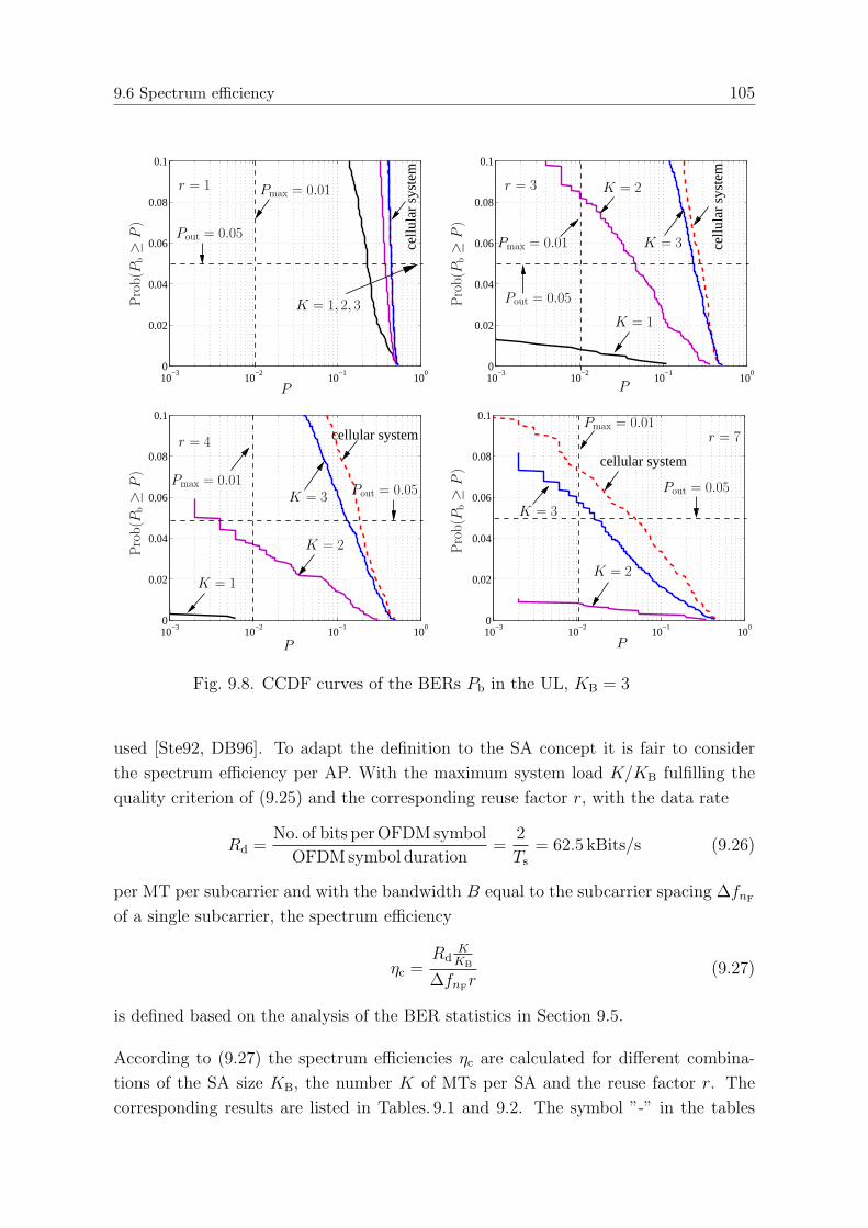
9.6 Spectrum efficiency 105
10−3
10−2
10−1
100
0
0.02
0.04
0.06
0.08
0.1
10−3
10−2
10−1
100
0
0.02
0.04
0.06
0.08
0.1
10−3
10−2
10−1
100
0
0.02
0.04
0.06
0.08
0.1
10−3
10−2
10−1
100
0
0.02
0.04
0.06
0.08
0.1
cellular system
cellu
lar
syst
em
cellu
lar
syst
em
cellular systemP
rob(P
b≥
P)
Prob(P
b≥
P)
P P
r = 1
K = 3
Pout = 0.05
Pout = 0.05
Pout = 0.05
PP
Pmax = 0.01
K = 3
r = 3
r = 4
Pout = 0.05
r = 7
K = 2
Pmax = 0.01
K = 1, 2, 3
K = 1
Pmax = 0.01 K = 3
K = 2
K = 1
K = 2
Pmax = 0.01
Prob(P
b≥
P)
Prob(P
b≥
P)
Fig. 9.8. CCDF curves of the BERs Pb in the UL, KB = 3
used [Ste92, DB96]. To adapt the definition to the SA concept it is fair to consider
the spectrum efficiency per AP. With the maximum system load K/KB fulfilling the
quality criterion of (9.25) and the corresponding reuse factor r, with the data rate
Rd =No. of bits per OFDM symbol
OFDM symbol duration=
2
Ts
= 62.5 kBits/s (9.26)
per MT per subcarrier and with the bandwidth B equal to the subcarrier spacing ∆fnF
of a single subcarrier, the spectrum efficiency
ηc =Rd
KKB
∆fnFr
(9.27)
is defined based on the analysis of the BER statistics in Section 9.5.
According to (9.27) the spectrum efficiencies ηc are calculated for different combina-
tions of the SA size KB, the number K of MTs per SA and the reuse factor r. The
corresponding results are listed in Tables. 9.1 and 9.2. The symbol ”-” in the tables

106 Chapter 9: Performance of JOINT in a multiple–service–area scenario
10−3
10−2
10−1
100
0
0.02
0.04
0.06
0.08
0.1
10−3
10−2
10−1
100
0
0.02
0.04
0.06
0.08
0.1
10−3
10−2
10−1
100
0
0.02
0.04
0.06
0.08
0.1
10−3
10−2
10−1
100
0
0.02
0.04
0.06
0.08
0.1
cellular system
cellu
lar
syst
em
cellu
lar
syst
em
cellular system
P P
P P
K = 1, 2, 3, 4
K = 2K = 3
Pout = 0.05
K = 2
K = 4Pout = 0.05
Pro
b(P
b≥
P)
Pro
b(P
b≥
P)
r = 1 r = 3
r = 4 r = 7
K = 3
Pmax = 0.01Pmax = 0.01
Pout = 0.05
Pmax = 0.01 K = 4 Pmax = 0.01
Pout = 0.05
K = 3
K = 4
K = 2
Pro
b(P
b≥
P)
Pro
b(P
b≥
P)
Fig. 9.9. CCDF curves of the BERs Pb in the DL, KB = 4
means that the corresponding case does not fulfill the criterion of (9.25). For the
optimum spectrum efficiency follows
ηc,op = maxK
KB,r
ηc, KB = 1, 3, 4, 7, . . . (9.28)
for each case of KB. As listed in Table. 9.3, it can be seen that the SA based JOINT has
a great potential for improving the spectrum efficiency ηc compared to the conventional
cellular system.

9.6 Spectrum efficiency 107
10−3
10−2
10−1
100
0
0.02
0.04
0.06
0.08
0.1
10−3
10−2
10−1
100
0
0.02
0.04
0.06
0.08
0.1
10−3
10−2
10−1
100
0
0.02
0.04
0.06
0.08
0.1
10−3
10−2
10−1
100
0
0.02
0.04
0.06
0.08
0.1
cellular system
cellu
lar
syst
em
cellular system
cellu
lar
syst
em
P P
Pro
b(P
b≥
P)
P P
r = 1 r = 3
r = 4 r = 7
K = 3, 4, 5, 6, 7
Pout = 0.05
Pout = 0.05K = 5
K = 7
Pmax = 0.01
K = 6
Pout = 0.05
K = 7
Pmax = 0.01
Pmax = 0.01 Pmax = 0.01
K = 6
K = 1
K = 5K = 4
K = 3
K = 6
K = 7
K = 2
Pout = 0.05
K = 4
Pro
b(P
b≥
P)
Pro
b(P
b≥
P)
Pro
b(P
b≥
P)
Fig. 9.10. CCDF curves of the BERs Pb in the DL, KB = 7
Table 9.1. Spectrum efficiencies ηc of the reference system of KB =1 and K = 1
r = 1 r = 3 r = 4 r = 7 r = 9 r = 12ηc
bits/s/Hz- - - - - 0.1333

108 Chapter 9: Performance of JOINT in a multiple–service–area scenario
Table 9.2. Spectrum efficiencies ηc of JOINT
KKB
= 13
r = 1 r = 3 r = 4 r = 7ηc
bits/s/Hz- 0.1778 0.1333 0.0762
KKB
= 23
r = 1 r = 3 r = 4 r = 7ηc
bits/s/Hz- - 0.2667 0.1524
KKB
= 33
r = 1 r = 3 r = 4 r = 7ηc
bits/s/Hz- - - -
KKB
= 14
r = 1 r = 3 r = 4 r = 7ηc
bits/s/Hz- 0.1333 0.1 0.0571
KKB
= 24
r = 1 r = 3 r = 4 r = 7ηc
bits/s/Hz- 0.2667 0.2 0.1143
KKB
= 34
r = 1 r = 3 r = 4 r = 7ηc
bits/s/Hz- - 0.3 0.1714
KKB
= 44
r = 1 r = 3 r = 4 r = 7ηc
bits/s/Hz- - - 0.2286
KKB
= 17
r = 1 r = 3 r = 4 r = 7ηc
bits/s/Hz0.2286 0.0762 0.0571 0.0327
KKB
= 27
r = 1 r = 3 r = 4 r = 7ηc
bits/s/Hz0.4571 0.1524 0.1143 0.0653
KKB
= 37
r = 1 r = 3 r = 4 r = 7ηc
bits/s/Hz- 0.2286 0.1714 0.098
KKB
= 47
r = 1 r = 3 r = 4 r = 7ηc
bits/s/Hz- 0.3048 0.2286 0.1306
KKB
= 57
r = 1 r = 3 r = 4 r = 7ηc
bits/s/Hz- 0.381 0.2857 0.1633
KKB
= 67
r = 1 r = 3 r = 4 r = 7ηc
bits/s/Hz- - 0.3429 0.1960
KKB
= 77
r = 1 r = 3 r = 4 r = 7ηc
bits/s/Hz- - - 0.2286
Table 9.3. Optimum spectrum efficiencies ηc,op
KB = 1 KB = 3 KB = 4 KB = 7ηc,op
bits/s/Hz0.1333 0.2667 0.3 0.4571

109
Chapter 10
Summaries
10.1 English
The thesis is focused on modelling and simulation of a Joint Transmission and De-
tection Integrated Network (JOINT), a novel air interface concept for B3G mobile
radio systems. Besides the utilization of the OFDM transmission technique, which is a
promising candidate for future mobile radio systems, and of the duplexing scheme time
division duplexing (TDD), the subdivision of the geographical domain to be supported
by mobile radio communications into service areas (SAs) is a highlighted concept of
JOINT. A SA consists of neighboring sub-areas, which correspond to the cells of con-
ventional cellular systems. The signals in a SA are jointly processed in a Central Unit
(CU) in each SA. The CU performs joint channel estimation (JCE) and joint detection
(JD) in the form of the receive-zero-forcing (RxZF) Filter for the uplink (UL) trans-
mission and joint transmission (JT) in the form of the transmit-zero-forcing (TxZF)
Filter for the downlink (DL) transmission. By these algorithms intra-SA multiple ac-
cess interference (MAI) can be eliminated within the limits of the used model so that
unbiased data estimates are obtained, and most of the computational effort is moved
from mobile terminals (MTs) to the CU so that the MTs can do with low complexity.
A simulation chain of JOINT has been established in the software MLDesigner by the
author based on time discrete equivalent lowpass modelling. In this simulation chain,
all key functionalities of JOINT are implemented. The simulation chain is designed
for link level investigations. A number of channel models are implemented both for
the single-SA scenario and the multiple-SA scenario so that the system performance of
JOINT can be comprehensively studied. It is shown that in JOINT a duality or a sym-
metry of the MAI elimination in the UL and in the DL exists. Therefore, the typical
noise enhancement going along with the MAI elimination by JD and JT, respectively,
is the same in both links. In the simulations also the impact of channel estimation
errors on the system performance is studied. In the multiple-SA scenario, due to the
existence of the inter-SA MAI, which cannot be suppressed by the algorithms of JD
and JT, the system performance in terms of the average bit error rate (BER) and the
BER statistics degrades. A collection of simulation results show the potential of JOINT
with respect to the improvement of the system performance and the enhancement of
the spectrum efficiency as compared to conventional cellular systems.

110 Chapter 10: Summaries
10.2 Deutsch
Obwohl Mobilfunksysteme der dritten Generation (3G) derzeit noch nicht auf Front
im Einsatz sind, sind bereits heute in vielen Teilen der Welt Forschungsaktivitaten
in Richtung von Mobilfunksystemen jenseits von 3G (Beyond 3G Systems, B3G) an-
gelaufen. Diese Aktivitaten sind nicht als verfruht zu bezeichnen, weil erfahrungs-
gemaß zwischen den ersten Schritten zur Entstehung eines neuen Mobilfunksystems bis
zu dessen endgultiger Inbetriebnahme durchaus ein Jahrzehnt oder mehr verstreichen
konnen. Ein wichtiger Aspekt bei der Konzeption von B3G-Mobilfunksystemen ist das
Ermoglichen wesentlich hoherer Datenraten als es die 2G- und 3G-Systeme gestatten.
Zunachst liegt es nahe, das Unterstutzen solch hoherer Datenraten ausschließlich durch
den Einsatz breiterer Frequenzbander zu ermoglichen. Weil allerdings Ubertragungs-
bandbreite auch kunftig ein kostbares Gut sein wird, erfordert das Unterstutzen solch
hoherer Datenraten eine moglichst effiziente Nutzung der Ressource Frequenzbereich,
d.h. eine moglichst hohe spektrale Effizienz. Die spektrale Effizienz kann durch Maß-
nahmen auf verschiedenen Ebenen des ISO/OSI-Referenzmodells gesteigert werden.
Grundsatzlich kann man unterscheiden zwischen Maßnahmen auf der physikalischen
Ebene, die in vorteilhafter Weise auf die Phanomene der Wellenausbreitung eingehen
und diese ausnutzen, und Maßnahme auf hoheren Ebenen, die auf eine moglichst opti-
male Nutzung der von der physikalischen Schicht bereitgestellten Ressourcen abzielen.
Bei einem ausgewogenen Systementwurf kommt es auf ein harmonisches Zusammen-
spiel dieser beiden Klassen von Maßnahmen an, wobei die physikalische Ebene als Basis
des Ganzen eine besondere Bedeutung hat. Die vorliegende Dissertation befaßt sich
mit einer neuen Architektur der physikalischen Ebene fur B3G-Mobilfunksysteme.
Bei der herkommlichen zellularen Struktur, wie man sie bei den heutigen 2G- und 3G-
Systemen vorfindet, sind die mobilen Terminale (MT) einer jeden Zelle im allgemeinen
exklusiv der Basisstation (BS) der betreffenden Zelle zugeordnet, wenn man von dem
gelegentlich verwendeten Verfahren der ”weichen” Ubergabe (engl. Soft Handoff) ab-
sieht. Diese strukturell einfache Art der Zuordnung ist vorteilhaft hinsichtlich des
erforderlichen Signalisierungsaufwands, hat jedoch einige gravierende Nachteile:
• In der Aufwartsstrecke treffen die von den MTs einer Zelle abgestrahlten Signale
nicht nur an der BS der eigenen Zelle ein, sondern unerwunschterweise auch an
den BSs anderer Zellen.
• In der Abwartsstrecke treten die von der BS abgestrahlten Signale nicht nur
an den der betreffenden BS zugeordneten MTs auf, sondern unerwunschterweise
auch an den MTs anderer BSs.

10.2 Deutsch 111
c o r e n e t w o r k
c e l l
B SM T
d a t a
Bild 10.1. Conventionalle zellulare Architektur, Beispiel mit 12 Zellen
Die genannten unerwunschten Signale wirken als Storung und werden als Vielfachzu-
griffsinterenferenz (engl. Multiple Access Interference, MAI) bezeichnet. Bei herkomm-
lichen Systemen kann die MAI aus anderen Zellen, die auch als Interzell-MAI bezeich-
net wird, nicht unterdruckt oder gar nutzbringend ausgewertet werden, was sich letzten
Endes schadlich auf die spektrale Effizienz auswirkt.
In der neuen Architektur, die in dieser Arbeit vorgeschlagen und untersucht wird,
geht es um die Milderung des genannten schadlichen Effekts der Interzell-MAI. Hierzu
werden in dem System anstelle der individuellen BSs Radiozugangspunkte (engl. Ac-
cess Point, AP) eingefuhrt, und Gruppen solcher APs werden mit einer der jeweiligen
Gruppe zugeordneten Zentraleinheit (engl. Central Unit, CU) verbunden, z.B. uber
Leitungen, Glasfasern oder mit Richtfunk. Der geographische Bereich um eine solche
Gruppe von APs bildet ein Servicegebiet (engl. Service Area, SA), und die MTs einer
jeden SA konnen mit der CU der SA uber die APs der SA kommunizieren. In den
Bildern 10.1 und 10.2 sind die konventionelle zellulare bzw. die neue SA-basierte Ar-
chitektur dargestellt, so daß ein Vergleich dieser beiden Architekturen moglich wird.
In der konventionelle zellularen Architektur nach Bild 10.1 kommunizieren die MTs
einer Zelle nur mit der BS ihrer Zelle, d.h. nur mit einem einzigen Funkzugangspunkt.
Die grundsatzliche Arbeitsweise der SA-basierten Architektur nach Bild 10.2 kann fol-
gendermaßen charakterisiert werden:

112 Chapter 10: Summaries
C UC U
c o r e n e t w o r k
S A
A PM T
C U
S A
S A
d a t a
Bild 10.2. Neue SA-basierte Architektur, Beispiel mit drei SAs
• In der Aufwartstrecke werden die Sendesignale der MTs der SA von allen APs
der SA empfangen und zur CU weitergeleitet, wo sie gemeinsam verarbeitet wer-
den. Das Ziel einer solchen gemeinsamen Verarbeitung besteht im Ausnutzen der
Empfangsleistungen aller APs derart, daß die gesamte abgestrahlte Leistung in
der SA und die Komplexitat der MTs klein gehalten werden konnen. Eine solche
gemeinsame Signalverarbeitung ist unter der Bezeichnung gemeinsame Detektion
(engl. Joint Detection, JD) bekannt und wird in abgewandelter Form auch schon
bei manchen 3G-Konzepten eingesetzt.
• In der Abwartsstrecke wird jede MT der SA durch die Sendesignale aller APs der
SA unterstutzt. Diese Signale werden in der CU gemeinsam erzeugt, und zwar
derart, daß die gesamte von den APs der SA abgestrahlte Sendeleistung moglichst
klein wird. Ein hierbei in der CU anwendbares Verfahren der Signalerzeugung
ist unter der Bezeichnung gemeinsames Senden (engl. Joint Transmission, JT)
bekannt und ist derzeit in verschiedenen Versionen ein weltweiter Gegenstand der
Forschung.
Weil der Einsatz von JD und JT wichtige Merkmale der vorgeschlagenen neuen SA-
basierten Architektur sind, wurde fur diese die Bezeichnung”
Joint Transmission and
Detection Integrated Network (JOINT)“ eingefuhrt.

10.2 Deutsch 113
Bei der herkommlichen zellularen Architektur nach Bild 10.1 kann man die MTs einer
Zelle durch den Einsatz entsprechender Vielfachzugriffsverfahren so versorgen, daß
keine gegenseitigen Storungen innerhalb der Zelle auftreten, d.h. daß es keine Intrazell-
MAI gibt. Bei dem Konzept JOINT konnen die MTs einer ganzen SA so versorgt wer-
den, daß man innerhalb einer jeden SA keine gegenseitigen Storungen durch Interferenz
hat, d.h. es gibt keine Intrazell-MAI. Ein Vergleich der Strukturen nach Bild 10.1 und
10.2 zeigt nun, daß bei der SA-basierten Architektur die Anzahl der interferenzfrei ver-
sorgbaren MTs wesentlich großer ist als bei der herkommlichen zellularen Architektur.
Dieser Sachverhalt ist der Grund fur die im SA-basierten Konzept erwartete hohere
spektrale Effizienz.
Im Rahmen der oben beschriebenen SA-basierten Architektur von JOINT hat man
beim Systementwurf zahlreiche Freiheitsgrade, z.B. hinsichtlich
• des Vielfachzugriffsverfahrens (FDMA, TDMA, CDMA, SDMA),
• des Ubertragungsmodus (Einzeltrager- oder Mehrtragerubertragung),
• des Duplexverfahrens (TDD oder FDD), und
• der Antennenanordnungen an den APs und den MTs (Einelement- oder Mehrele-
mentantennen).
Vor dem Hintergrund dieser Freiheitsgrade wird in der vorliegenden Arbeit eine gewisse
Auswahl getroffen, die sich an den Rahmenbedingungen orientiert, die sich derzeit in
der B3G-Standardisierung abzeichnen. Folgendes wird fur die Untersuchungen in dieser
Arbeit ausgewahlt:
• Vielfachzugriffsverfahren: SDMA,
• Ubertragungsmodus: Mehrtragerubertragung, speziell OFDM,
• Duplexverfahren:TDD,
• Antennenanordnung: Ein- oder Mehrelementantennen an den APs, Einelemen-
tantennen an den MTs.
Im folgenden wird diese Auswahl kurz begrundet. Das Vielfachzugriffsverfahren SDMA
ist ein naheliegendes Trennverfahren fur raumlich dislozierte MTs, die mit einer An-
zahl raumlich ebenfalls dislozierter APs kommunizieren, wie es bei JOINT der Fall
ist. Auf den Ubertragungsmodus OFDM, der im ubrigen ganz generell ein Favorit

114 Chapter 10: Summaries
im Bereich B3G ist, fiel die Wahl wegen seiner Flexibilitat und seines Potentials einer
niedrigen Sender- und Empfangerkomplexitat. Das Duplexverfahren TDD wurde aus-
gewahlt, weil es Anwendungen mit stark unterschiedlicher Datenraten in Auf- und
Abwartsstrecke unterstutzt; mit FDD konnte man solche Asymmetrien nicht ohne
weiteres bewaltigen. Uberdies ermoglicht TDD Vereinfachungen beim Beschaffen der
in der CU fur die Algorithmen JD und JT erforderlichen Kanalinformation, weil man
die Reziprozitat der gleichfrequenten Funkkanale von Auf- und Abwartsstrecke aus-
nutzen kann.
Der Entwurf und die Entwicklung von Mobilfunksystemen auf der Grundlage des
Konzepts JOINT ist aufgrund der zu bewaltigenden Komplexitat, der vielfaltigen
Moglichkeiten der Parameterwahl und der vielen zu beachtenden Randbedingun-
gen eine sehr anspruchsvolle Aufgabe. Diese Aufgabe kann weder allein durch
geschlossene Systemberechnungen noch durch Messungen an realisierten Hardware-
Funktionsmustern bewaltigt werde. Vielmehr ist als eine wesentliche Komponente
bei solchen Arbeiten die Systemsimulation auf dem Rechner erforderlich. Hierzu
benotigt man hinreichend genaue mathematische Modelle handhabbarer Komplexitat
aller Systemkomponenten wie z.B. Sender, Empfanger, Antennen, Ubertragungskanale
etc. Weiterhin benotigt man, um den eigenen Programmieraufwand in Grenzen zu
halten, ein moglichst komfortables und flexibles kommerzielles Simulationswerkzeug.
Gegenstand der vorliegenden Arbeit sind die Modellierung und Simulation SA-basierter
Ubertragungssysteme nach dem Konzept JOINT. Als Werkzeug zum Losen dieser Auf-
gaben hat die Verfasserin das Werkzeug MLDesigner ausgewahlt. Mit den Ergebnis-
sen ihrer Arbeit hat sie auch zur Weiterentwicklung von JOINT beigetragen, wobei
erwahnt werden sollte, daß die Grundlagen der in JOINT verwendeten Algorithmen
fur die Kanalschatzung sowie zum Durchfuhren von JD und JT in zwei anderen Pro-
motionsvorhaben gelegt wurden. Das primares Anliegen in der vorliegenden Arbeit
ist das Aufbereiten von JOINT fur die Simulationen und das Gewinnen quantitativer
Ergebnisse zur Performanzevaluierung und gunstigen Parametrisierung von JOINT.
In Systemen wie JOINT senden und empfangen eine Vielzahl von MTs information-
stragende Signale uber die zeitvarianten und frequenzselektiven Ubertragungskanale
zwischen den MTs und den APs. Die daraus resultierende gegenseitige Storung der
einzelnen Verbindungen (engl. Muliple Access Interference, MAI) ist der wesentliche
Grund fur die Begrenztheit der spektralen Effizienz. Bei der Modellierung und Simula-
tion von JOINT spielen deshalb das quantitative Ermitteln und moglichst weitgehende
Eliminieren solcher Interferenzen durch JD bzw. JT eine zentrale Rolle. Wichtige
durch die Simulation zu beantwortende Fragen betreffen
• die Performanz von JOINT in Auf- und Abwartsstrecke einer isolierten SA unter

10.2 Deutsch 115
der Voraussetzung perfekter Kanalkenntnis,
• die Auswirkungen nicht perfekter Kanalkenntnis auf die Performanz einer
isolierten SA,
• die Auswirkungen von Inter-SA-MAI im Falle eines Verbandes von mehreren SAs.
Kapitel 1 ist die Einleitung der Arbeit. In Kapitel 2 werden die fur die Simulation
erstellten Kanalmodelle vorgestellt. Kapitel 3 ist der detaillierten mathematischen
Modellierung von JOINT gewidmet. Zum Beschreiben von Signalen und Operatio-
nen im zeitdiskreten aquivalenten Tiefpaßbereich werden hierbei Vektoren bzw. Ma-
trizen eingefuhrt. In diesem Kapitel werden auch die bei den spateren Simulatio-
nen gewahlten Parametersatze zusammengestellt. Kapitel 4 ist speziell dem Prob-
lem der Kanalschatzung in JOINT und der Modellierung des entsprechenden Algo-
rithmus JCE (Joint Channel Estimation) gewidmet. Kapitel 5 befaßt sich mit der
mathematischen Modellierung des in der Aufwartsstrecke von JOINT zu wahlenden
Signalverarbeitungsalgorithmus JD. Hierbei wird auch das Performanzkriterium SNR-
Degradation eingefuhrt, das zum quantitativen Bewerten des durch die Simulationen
ermittelten Systemverhaltens geeignet ist. In Kapitel 6 wird in entsprechender Weise
der in der Abwartsstrecke von JOINT zu wahlende Algorithmus JT mathematisch mod-
elliert; weiterhin wird in diesem Kapitel ein der SNR-Degradation der Aufwartsstrecke
entsprechendes Performanzkriterium eingefuhrt. Dieses Kriterium wird als Sende-
effizienz bezeichnet und ist ein Maß fur die zum Erzielen einer bestimmten Emp-
fangsqualitat erforderliche Sendeleistung in der SA. Kapitel 7 gibt einen umfassenden
Uberblick uber die Implementierung der JOINT-Simulationskette mit dem Werkzeug
MLDesigner. Hierbei wird auf moglichst große Flexibilitat der Simulationskette abge-
hoben. Flexibiltat wird durch eine konsequente modulare Anordnung und komfortable
Parametereinstellmoglichkeiten erzielt, so daß eine leichte Austauschbarkeit von Simu-
lationsmodulen und ein muheloser Wechsel von Parametern gewahrleistet. In Kapitel
8 werden umfangreiche Simulationsergebnisse zur Performanz der Aufwartstrecke und
der Abwartsstrecke in einer isolierten SA von JOINT prasentiert. Besonderes Au-
genmerk wird hierbei auf den Einfluß einer fehlerbehafteten Kanalschatzung auf das
Systemverhalten gelegt. Kapitel 9 ist schließlich Simulationsergebnissen zum Verhalten
von JOINT in einem Verbund mehrerer SAs gewidmet. Es werden Fehlerwahrschein-
lichkeiten sowie Wahrscheinlichkeitsdichteverteilungen von Fehlerwahrscheinlichkeiten
ermittelt. Auf der Grundlage dieser Ergebnisse kann dann die spektrale Effizienz kon-
ventioneller zellularer Systeme und SA-basierter Systeme nach dem Konzept JOINT
vergleichen werden. Bei den Simulationen zeigte sich, daß die spektrale Effizienz beim
Konzept JOINT je nach Parametrisierung zwei bis drei mal hoher ist als beim kon-
ventionellen zellularen Konzept. Dieser Vergleich zeigt eindrucksvoll das vorteilhafte

116 Chapter 10: Summaries Abschneiden von JOINT. 10.3 Chinese 本篇论文的重点是对 JOINT(Joint Transmission and Detection Integrated Network),即
联合传输与检测集成网络系统,进行建模与仿真。JOINT 着眼于超三代(Beyond 3G,
B3G)移动通讯系统,是一项崭新的空间接口技术。在性能优越的正交频分复用
(Orthogonal Frequency Division Multiplexing, OFDM)传输技术的基础上,JOINT 采用
了时分复用(Time Devision Duplex, TDD)模式。另外,JOINT 以传统的蜂窝小区(cell)
的概念为基础,对移动通讯系统所覆盖的区域重新进行划分,所形成的服务区
(service areas, SAs)的概念,在 JOINT 中最为引人注目。一个 SA 由相邻的若干子服
务区(sub-areas)构成,其中,sub-areas 在概念上对应于传统蜂窝移动系统中的 cells。
在同一个 SA 内的信号将由该 SA 中的中央控制区(central unit, CU)联合处理。在上行
链路(uplink, UL)中,CU 执行联合信道检测(joint channel estimation, JCE)算法以及联
合数据检测(joint detection, JD)算法;在下行链路(downlink, DL)中,CU 执行联合数
据传输(joint transmission, JT)算法。其中,处于接收端的 JD 和处于发送端的 JT 都采
用了强制归零(zero forcing, ZF)算法。通过上述技术在系统中的应用,可以有效地抑
制同一 SA 内多址干扰(intra-SA multiple access interference, intra-SA MAI)的影响,从
而实现无偏数据估计。与此同时,主要的、复杂的信号处理任务都由 CU 承担,因
此移动终端 (mobile terminals, MTs)可以保持轻便的设计。作者在仿真软件
MLDesigner 中完成了对 JOINT 系统的设计与实现。全部关键组件都是建立在时域离
散等效低通的模型基础上,为链路层仿真所设计,适用于单服务区(single-SA)与多
服务区(multiple-SA)、以及不同的信道模型的情况。通过研究发现,在 single-SA 的
情况下,系统在 UL 和 DL 中呈现出某种对称性,即在抑制 intra-SA MAI 方面,JD
和 JT 要付出相同的代价。另外,本文还研究了信道估计的误差对系统性能造成的影
响。针对 multiple-SA 的情况,由于来自其他同频服务区的干扰(inter-SA MAI)无法
通过上述 JD 和 JT 算法消除,系统性能将会有所降低。对仿真结果,特别是关于平
均误码率(bit error rate, BER)和 BER 的统计特性的分析表明,与传统的蜂窝式系统结
构相比,基于 SA 概念上的 JOINT 系统,在提高系统性能和增进频谱利用率等方面
具有很大的潜力,具有非常好的研究与开发前景。

117
Appendix A
Positions of access points and mobileterminals of Section 9.2
A.1 Preliminary remarks
The method to implement the multiple–SA scenarios described in Section 9.2 is dis-
cussed in the following. Since the shape of the sub–areas, which form the SA, is
hexagonal, the shape of the SAs might become non–hexagonal. Moreover, the shape
of the clusters of the SAs might be non–hexagonal as well. These facts will make the
implementation of the scenarios more difficult, especially to locate the APs and the
MTs of the co–channel SAs. In the following, with the aid of hierarchical–diamond
grids, the positions of the APs and the MTs in the co–channel SAs are generated step
by step.
A.2 Positions of access points
A.2.1 Positions of reference access points in co–channel ser-vice areas
The positions of the APs in the sub–areas, of the reference APs in the SAs, and of
the reference APs in the co–channels SAs are located along three hierarchical–diamond
grids, respectively.
At the first level, the APs of all the hexagonal sub–areas are located along the diamond
grid, as depicted in Fig.A.1. With R denoting the radius of the hexagonal sub–areas
the distance
D1 =√
3R (A.1)
between the neighboring points along the grid can be obtained for the first–level grid.
The rotation angle ϕ1 is defined as the angle between the unit vector−→l1 of the first–
level grid and the dashed reference line (RL). E.g., in Fig.A.1 with the initial angle
θ1
ϕ1 = θ1 (A.2)

118 A: Positions of access points and mobile terminals of Section 9.2
holds, where θ1 is usually assumed to be zero. With (A.1) and (A.2) the two unit
vectors of the grid can be expressed as
−→l1 =
(D1 cos ϕ1
D1 sin ϕ1
)=
( √3R cos θ1√3R sin θ1
)(A.3)
and−→l2 =
(D1 cos
(ϕ1 + π
3
)D1 sin
(ϕ1 + π
3
))
=
( √3R cos
(θ1 + π
3
)√
3R sin(θ1 + π
3
))
(A.4)
so that the first–level grid can be totally determined.
RL
ϕ1 = θ1
π
3
D1
R
−→l2 −→
l1
Fig. A.1. First–level grid of all the APs in the sub–areas
RL
π3
−→m2
D2−→m1
ϕ2 = θ1 + θ2θ2 θ2i1D1
j1D12
3π
D2
θ1
Fig. A.2. Second–level grid of the reference APs in all the SAs
On the second level, the grid, along which the reference APs of all the SAs are located,
can be obtained based on the first–level grid. In the scenarios with the hexagonal
sub–areas the SA size reads
KB = i21 + j21 + i1j1, with i1, j1 ∈ N0, i1 + j1 6= 0. (A.5)

A.2 Positions of access points 119
RL
θ2
π3
−→n2
D3
θ3
θ3
2
3π
−→n1
D3
i2D2
j2D2
θ1
ϕ3 = θ1 + θ2 + θ3
Fig. A.3. Third–level grid of the reference APs in the co–channelSAs
With (A.1) the distance
D2 =√
KBD1 =√
3KBR (A.6)
between the neighboring points along the grid can be obtained for the second–level grid.
In the triangle depicted on the right of Fig. A.2, according to the geometry property of
triangles [Ton56],
(j1D1)2 = D2
2 + (i1D1)2 − 2D2 · i1D1 cos θ2 (A.7)
holds. With (A.7) the additional rotation angle
θ2 = arccos
(2i1 + j1
2√
i21 + j21 + i1j1
)(A.8)
is obtained. For the rotation angle on the second level follows
ϕ2 = θ1 + θ2. (A.9)
Therefore, with (A.6) and (A.9), the two unit vectors of the second level grid can be
expressed as
−→m1 =
(D2 cos ϕ2
D2 sin ϕ2
)=
( √3KBR cos (θ1 + θ2)√3KBR sin (θ1 + θ2)
)(A.10)
and
−→m2 =
(D2 cos
(ϕ2 + π
3
)D2 sin
(ϕ2 + π
3
))
=
( √3KBR cos
(θ1 + θ2 + π
3
)√
3KBR sin(θ1 + θ2 + π
3
))
(A.11)
so that the second–level grid can be totally determined.

120 A: Positions of access points and mobile terminals of Section 9.2
π3 ϕ3 = θ1 + θ2 + θ3
D3
(x(4,1), y(4,1))
y
x
Fig. A.4. Positions (x(i,j), y(i,j)) of the reference APs in the co–channel SAs
On the third level, the grid, along which the reference APs of the co–channel SAs are
located, can be obtained based on the second–level grid. In the scenarios with the
hexagonal sub–areas the reuse factor reads
r = i22 + j22 + i2j2, with i2, j2 ∈ N0, i2 + j2 6= 0. (A.12)
Therefore, with (A.6) the distance
D3 =√
rD2 =√
3KBrR (A.13)
between the neighboring points along the grid can be obtained for the third–level grid.
In the triangle depicted on the right of Fig. A.2, according to the geometry property of
triangles [Ton56],
(j2D2)2 = D2
3 + (i2D2)2 − 2D3 · i2D2 cos θ3 (A.14)
holds. With (A.14) the additional rotation angle
θ3 = arccos
(2i2 + j2
2√
i22 + j22 + i2j2
)(A.15)
on the third level is obtained. For the rotation angle on the third level follows
ϕ3 = θ1 + θ2 + θ3. (A.16)
With (A.13) and (A.16), the two unit vectors of the third level grid can be expressed
as−→n1 =
(D3 cos ϕ3
D3 sin ϕ3
)=
( √3KBrR cos (θ1 + θ2 + θ3)√3KBrR sin (θ1 + θ2 + θ3)
)(A.17)

A.3 Positions of mobile terminals 121
and
−→n2 =
(D3 cos
(ϕ3 + π
3
)D3 sin
(ϕ3 + π
3
))
=
( √3KBrR cos
(θ1 + θ2 + θ3 + π
3
)√
3KBrR sin(θ1 + θ2 + θ3 + π
3
))
(A.18)
so that the third–level grid can be totally determined.
An arbitrary reference AP, as well as the corresponding SA, can be denoted by a pair
of integers (i, j) on the third–level grid, e.g., the indicated reference AP in Fig.A.4 is
denoted by (4, 1). With (A.13) and (A.16) the reference AP (i, j) on the third–level
grid can be represented with the Cartesian coordinates(
x(i,j)
y(i,j)
)= jD3
(sin(π
6− ϕ3)
cos(π6− ϕ3)
)+ iD3
(cos ϕ3
sin ϕ3
)
=√
3KBrR
(j sin(π
6− ϕ3) + i cos ϕ3
j cos(π6− ϕ3) + i sin ϕ3
). (A.19)
A.2.2 Positions of other access points in co–channel serviceareas
To locate all the APs in the co–channel SAs, it is necessary to know first the positions
of the APs kB, kB = 1 . . . KB, in the SA (0,0). Fig.A.5 depicts the positions of the
KB APs in some cases of different SA sizes KB. With (A.19) the position of the AP
kB, kB = 1 . . . KB, in the co–channel SA (i, j) can be calculated by(
x(i,j, kB)AP
y(i,j, kB)AP
)=
(x
(0,0, kB)AP
y(0,0, kB)AP
)+
(x(i,j)
y(i,j)
). (A.20)
A.3 Positions of mobile terminals
In [Meu98] the algorithm of generating a random position with uniform distribution in
a hexagon was introduced. In this algorithm, a random position (xrand, yrand), which is
uniformly distributed in an equilateral triangle, one of the six components forming the
hexagon, is first generated, as depicted in Fig.A.6. Then, by rotation five positions in
the other five equilateral triangles can be obtained. Finally, one of the six positions is
chosen as the random desired position.
With the aid of the random position (xrand, yrand) generated by
yrand =
√3
2R(1−√u), u ∈ [0, 1], (A.21)

122 A: Positions of access points and mobile terminals of Section 9.2
KB = 1
KB = 3
KB = 7KB = 4
(0, 0)
(0, 0) (0, 0)
(0, 0)
(
√3R2
, 32R)
(√
3R, 0)
(−√
3R2
, 32R) (
√3R2
, 32R)
(√
3R, 0)(−√
3R, 0)(√
3R, 0)
(
√3R2
,−32R) (
√3R2
,−32R)(−
√3R2
,−32R)
(
√3R2
, 32R)
Fig. A.5. Positions (x(0,0, kB)AP , y
(0,0, kB)AP ) of the APs kB, kB =
1 . . . KB, in the SA (0,0), for different SA sizes KB
R
(xrand, yrand)
Fig. A.6. Generation of random positions in a hexagon with theaid of a random position (xrand, yrand) in the dashed–linetriangle
and
xrand =R
2+ (v − 1
2)
(R− 2√
3yrand
), v ∈ [0, 1], (A.22)
in the equilateral triangle depicted in Fig.A.6, where random variables u and v are
uniformly distributed in the interval [0, 1], with m denoting an integer randomly dis-
tributed in the set {0, 1, 2, 3, 4, 5} [Meu98] and with (A.20), a possible position
(x
(i,j, k)MT
y(i,j, k)MT
)=
(cos(mπ
3+ π
6) − sin(mπ
3+ π
6)
sin(mπ3
+ π6) cos(mπ
3+ π
6)
)(xrand
yrand
)+
(x
(i,j, kB)AP
y(i,j, kB)AP
)(A.23)
of the MT k, in the sub–area, at whose center the AP kB is located, in the co–channel
SA (i, j) [Meu98].

123
List of frequently used abbreviations andsymbols
Abbreviations
2G / 3G 2nd Generation / 3rd Generation
AP access point
B3G beyond 3 Generation
BER bit error rate
CCDF complementary cumulative distribution function
CDMA code division multiple access
CIR channel impulse response
CSI channel state information
CTF channel transfer function
CU central unit
DL downlink
JCE joint channel estimation
JD joint detection
JOINT Joint Transmission and Detection Integrated Network
JT joint transmission
LTS linear transmission system
MA multiple access
MAI multiple access interference
MF matched filter
MIMO multiple input multiple output
ML maximum likelihood
MT mobile terminal
MUD multiuser detection
OFDM orthogonal frequency division multiplexing
SA service area
SNR signal–to–noise ratio
TDD Time Division Duplexing
TxZF transmit zero forcing
UL uplink
ZF zero forcing

124 List of frequently used abbreviations and symbols
Symbols
B system bandwidth
Bc coherence bandwidth
c0 speed of light in the vacuum
d(k)
nFdata symbol of the MT k on the subcarrier nF in the general
transmission modelˆd(k)
nFestimate of the data symbol d
(k)
nF
d(k)
d, nFDL data symbol of the MT k on the subcarrier nF
ˆd(k)d, nF
estimate of the data symbol d(k)
d, nF
d(k)
d, nB, nFDL data symbol of the MT k on the subcarrier nF at the time slot nB
d(k)
u, nFUL data symbol of the MT k on the subcarrier nF
ˆd(k)u, nF
estimate of the data symbol d(k)
u, nF
d(k)
u, nB, nFUL data symbol of the MT k on the subcarrier nF at the time slot nB
dnFsubcarrier–specific data vector in the general transmission model
ˆdnFestimate vector of the subcarrier–specific data vector dnF
in the general
transmission model
dd DL total data vector
dd, nFsubcarrier–specific DL data vector
ˆdd, nFestimate vector of the subcarrier–specific DL data vector dd, nF
dd, mul, nFsubcarrier–specific DL data vector in the multiple–SA scenario
dd, nB, nFslot–subcarrier–specific DL data vector
d(nSA)
d, nFsubcarrier–specific DL data vector of the SA nSA
ˆd(nSA)
d, nFestimate vector of the subcarrier–specific DL data vector d
(nSA)
d, nF
du total UL data vector
du, nFsubcarrier–specific UL data vector
ˆdu, nFestimate vector of the subcarrier–specific UL data vector du, nF
du, mul, nFsubcarrier–specific UL data vector in the multiple–SA scenario
du, nB, nFslot–subcarrier–specific UL data vector
d(nSA)
u, nFsubcarrier–specific UL data vector of the SA nSA
ˆd(nSA)
u, nFestimate vector of the subcarrier–specific UL data vector d
(nSA)
u, nF
DnFsubcarrier–specific detector matrix in the general transmission model
Dd, nFsubcarrier–specific DL detector matrix
Du, nFsubcarrier–specific UL detector matrix
e(kB)d, nF
DL receive value of the AP kB on the subcarrier nF
e(k)u, nF
UL data symbol of the MT k on the subcarrier nF
ed total DL receive vector

List of frequently used abbreviations and symbols 125
ed, nFsubcarrier–specific DL receive vector
e(nSA)d, nF
subcarrier–specific DL receive vector of the SA nSA
ed, mul, nFsubcarrier–specific DL receive vector in the multiple–SA scenario
eu total UL receive vector
eu, nFsubcarrier–specific UL receive vector
e(nSA)u, nF
subcarrier–specific UL receive vector of the SA nSA
eu, mul, nFsubcarrier–specific UL receive vector in the multiple–SA scenario
Ed data symbol energy
Ep pilot symbol energy
EnB, nFCTF estimation error matrix of the time slot nB on the subcarrier nF
fc carrier frequency
fd, max maximum Doppler frequency
∆fnFsubcarrier spacing
F noise figure
FdB logarithmic noise figure
F Fourier transform matrix
FW, tot total Fourier transform matrix
g(t) linear path gain
G(t) logarithmic path gain
G average logarithmic path gain
gR antenna gain at the receiver
gT antenna gain at the transmitter
h(k, kB)w w–th tap CIR between the MT k and the AP kB
h(k, kB)
w estimate of the CIR h(k, kB)w
h(k, kB)
nFCTF between the MT k and the AP kB on the subcarrier nF
ˆh(k, kB)
nFestimate of the CTF h
(k, kB)
nF
h(k, kB)
nB, nFslot–specific CTF between the MT k and the AP kB on the
subcarrier nF
ˆh(k, kB)
nB, nFestimate of the slot–specific CTF h
(k, kB)
nB, nF
the subcarrier nF
h(t) time continuous CIR vector
h(t) time continuous CTF vector
h(kB) AP–specific CIR vector
h(kB)
estimate vector of the AP–specific CIR vector h(kB)
h(kB)
AP–specific CTF vector
ˆh(kB)
estimate vector of the AP–specific CTF vector h(kB)
HnFsubcarrier–specific CTF matrix in the general transmission model
Hd DL CTF matrix
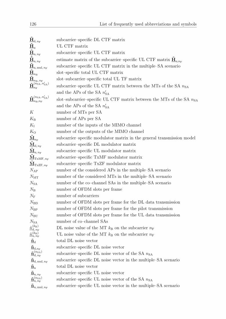
126 List of frequently used abbreviations and symbols
Hd, nFsubcarrier–specific DL CTF matrix
Hu UL CTF matrix
Hu, nFsubcarrier–specific UL CTF matrix
ˆHu, nFestimate matrix of the subcarrier–specific UL CTF matrix Hu,nF
Hu, mul, nFsubcarrier–specific UL CTF matrix in the multiple–SA scenario
HnBslot–specific total UL CTF matrix
HnB, nFslot–subcarrier–specific total UL TF matrix
H(nSA, n′SA)
nFsubcarrier–specific UL CTF matrix between the MTs of the SA nSA
and the APs of the SA n′SA
H(nSA, n′SA)
nB,nFslot–subcarrier–specific UL CTF matrix between the MTs of the SA nSA
and the APs of the SA n′SA
K number of MTs per SA
KB number of APs per SA
KI number of the inputs of the MIMO channel
KO number of the outputs of the MIMO channel
MnFsubcarrier–specific modulator matrix in the general transmission model
Md, nFsubcarrier–specific DL modulator matrix
Mu, nFsubcarrier–specific UL modulator matrix
MTxMF, nFsubcarrier–specific TxMF modulator matrix
MTxZF, nFsubcarrier–specific TxZF modulator matrix
NAP number of the considered APs in the multiple–SA scenario
NMT number of the considered MTs in the multiple–SA scenario
NSA number of the co–channel SAs in the multiple–SA scenario
NB number of OFDM slots per frame
NF number of subcarriers
NBD number of OFDM slots per frame for the DL data transmission
NBP number of OFDM slots per frame for the pilot transmission
NBU number of OFDM slots per frame for the UL data transmission
NSA number of co–channel SAs
n(kB)d, nF
DL noise value of the MT kB on the subcarrier nF
n(kB)u, nF
UL noise value of the MT kB on the subcarrier nF
nd total DL noise vector
nd,nFsubcarrier–specific DL noise vector
n(nSA)d, nF
subcarrier–specific DL noise vector of the SA nSA
nd, mul, nFsubcarrier–specific DL noise vector in the multiple–SA scenario
nu total DL noise vector
nu, nFsubcarrier–specific UL noise vector
n(nSA)u, nF
subcarrier–specific UL noise vector of the SA nSA
nu, mul, nFsubcarrier–specific UL noise vector in the multiple–SA scenario

List of frequently used abbreviations and symbols 127
p(k)
nFpilot symbol for the MT k on the subcarrier nF
p(k) MT–specific pilot vector
P(k)
MT–specific pilot matrix
P total pilot matrix
P(k)b, d, nF
bit error probability of the DL data symbol d(k)
d, nF
P(k)b, d, nB, nF
bit error probability of the DL data symbol d(k)
d, nB, nF
P(k)b, u, nF
bit error probability of the UL data symbol d(k)
u, nF
P(k)b, u, nB, nF
bit error probability of the UL data symbol d(k)
u, nB, nF
r reuse factor
R radius of the hexagonal sub–area
Rd data rate per MT per subcarrier
R(k)d, nF
useful receive energy of the DL data symbol d(k)
d, nF
R(k)TxMF, nF
useful receive energy of the DL data symbol d(k)
d, nFwith TxMF
R(k)TxZF, nF
useful receive energy of the DL data symbol d(k)
d, nFwith TxZF
Rd, d covariance matrix of the data vector dd, nF
Rd, u covariance matrix of the data vector du, nF
Rn, d covariance matrix of the noise vector nd, nF
Rn, u covariance matrix of the noise vector nu, nF
R∆ covariance matrix of the data estimation error vector ∆nFin the
general transmission model
R∆, d covariance matrix of the DL data estimation error vector ∆d, nB, nF
R∆, u covariance matrix of the UL data estimation error vector ∆u, nB, nF
s(kB)d, nF
DL transmit symbol of the AP kB on the subcarrier nF
s(k)u, nF
UL transmit symbol of the MT k on the subcarrier nF
sd DL total transmit vector
sd,nFsubcarrier–specific DL transmit vector
sd, mul, nFsubcarrier–specific DL transmit vector in the multiple–SA scenario
s(nSA)d, nF
subcarrier–specific DL transmit vector of the SA nSA
su UL total transmit vector
su, nFsubcarrier–specific UL transmit vector
su, mul, nFsubcarrier–specific UL transmit vector in the multiple–SA scenario
s(nSA)u, nF
subcarrier–specific UL transmit vector of the SA nSA
T average transmit data symbol energy
TdBm average transmit data symbol energy in dBm
Tcp cyclic prefix duration
Ts OFDM symbol duration
Toss OFDM symbol slot duration
Tfr OFDM frame duration

128 List of frequently used abbreviations and symbols
Td total transmit anergy
Tk correlation duration
T(k)nF transmit energy invested for the data symbol d
(k)
nFin the general
transmission model
T(k)d, nF
transmit energy invested for the DL data symbol d(k)
d, nF
T(k)u, nF transmit energy invested for the UL data symbol d
(k)
u, nF
T(k)TxMF, nF
transmit energy invested for the DL data symbol d(k)
d, nFwith TxMF
T(k)TxZF, nF
transmit energy invested for the DL data symbol d(k)
d, nFwith TxZF
vmax maximum velocity of MTs
W dimension of the CIR vector
α1 the first attenuation exponent in the dual–slope model
α2 the second attenuation exponent in the dual–slope model
γ(k)nF SNR of the data symbol d
(k)
nFin the general transmission model
γ(k)d, nF
SNR of the DL data symbol d(k)
d, nF
γ(k)u, nF SNR of the UL data symbol d
(k)
u, nF
γ(k)MF, nF
SNR of the UL data symbol d(k)
u, nFwith RxMF
γ(k)ZF, nF
SNR of the UL data symbol d(k)
u, nFwith RxZF
δ(k)nF SNR degradation of the data symbol d
(k)
nFin the general transmission
model
∆(kB)h, n AP–specific CTF estimation error vector due to the noise
∆(kB)h, nB
AP–specific CTF estimation error vector due to the time variance
∆d, nB, nFsubcarrier–specific DL data estimation error vector
∆u, nB, nFsubcarrier–specific UL data estimation error vector
ηc spectral efficiency
ηc, op optimum spectral efficiency
η(k)Tx, nF
efficiency of the data symbol d(k)
nFat the transmitter side in the general
transmission model
η(k)Rx, nF
efficiency of the data symbol d(k)
nFat the receiver side in the general
transmission model
η(k)Tx, d, nF
efficiency of the DL data symbol d(k)
d, nFat the transmitter side
η(k)Tx,u, nF
efficiency of the UL data symbol d(k)
u, nFat the transmitter side
η(k)Rx,d, nF
efficiency of the DL data symbol d(k)
d, nFat the receiver side
η(k)Rx,u, nF
efficiency of the UL data symbol d(k)
u, nFat the receiver side
ε(k)nF overall energy efficiency of the data symbol d
(k)
nFin the general
transmission model
ε(k)d, nF
overall energy efficiency of the DL data symbol d(k)
d, nF
ε(k)u, nF overall energy efficiency of the UL data symbol d
(k)
u, nF

List of frequently used abbreviations and symbols 129
κ Bolzmann’s constant
ρ distance between the transmitter and the receiver
ρB break–even–point distance
σ2 variance of real and imaginary parts of noise
σ2h, n variance of the CTF estimation errors due to the noise
σ2h, tv variance of the CTF estimation errors due to the time variance
ρB break–even–point distance
τmax maximum delay
τmin minimum delay
τh excess delay
τsup supremum of maximum delays

130
Literature
[BARY96] Bach Andersen, J.; Rappaport, T. S.; Yoshida, S.: Propagation measure-ments and models for wireless communications channels. IEEE Commu-nications Magazine, vol. 34, 1996, pp. 42–49.
[Bin90] Bingham, J. A. C.: Multicarrier modulation for data transmission: Anidea whose time has come. IEEE Communications Magazine, vol. 28,1990, pp. 5–14.
[Bin91] Bingham, J.: ADSL, VDSL and Multicarrier Modulation. New York:John Wiley & Sons, 1991.
[Bla98] Blanz, J. J.: Empfangsantennendiversitat in CDMA-Mobilfunksystemenmit gemeinsamer Detektion der Teilnehmersignale. FortschrittberichteVDI, Reihe 10, No. 535. Dusseldorf: VDI-Verlag, 1998.
[BMWT00] Baier, P. W.; Meurer, M.; Weber, T.; Troger, H.: Joint transmission(JT), an alternative rationale for the downlink of time division CDMAusing multi-element transmit antennas. Proc. IEEE 6th InternationalSymposium on Spread Spectrum Techniques & Applications (ISSSTA’00),vol. 1, Parsippany, 2000, pp. 1–5.
[Cim85] Cimini, L.: Analysis and simulation of a digital mobile channel usingorthogonal division frequency multiplexing. IEEE Transactions on Com-munications, vol. 33, 1985, pp. 665–675.
[COS89] COST 207: Digital land mobile radio communications. Final Report, Of-fice for Official Publications of the European Communities, Luxemburg,1989.
[COS91] COST 231: Urban Transmission Loss Models for Mobile Radio in the900- and 1800- MHz Bands. Technical Report COST 231 TD (91) (119,Rev. 2), COST 231, 1991.
[Cou97] Couch, L. W.: Digital and Analog Communication Systems, 5th Edition.Prentice-Hall International, 1997.
[CTC91] Chow, P.; Tu, J.; Cioffi, J.: Performance evaluation of a multichan-nel tranceiver system for ADSL and VHDSL services. IEEE Journal onSelected Areas in Communications, vol. 9, 1991, pp. 909–919.
[CWKS97] Chow, P.; Widjada, I.; Kim, J.; Sakai, P.: IEEE 802.11 wireless local areanetworks. IEEE Communications Magazine, vol. 9, 1997, pp. 116–126.
[DB96] David, K.; Benkner, T.: Digitale Mobilfunksysteme. Stuttgart: B. G.Teubner, 1996.
[Doe57] Doelz, M.: Binary Data Transmission Technique for Linear Systems.Proc. IRE, 1957, pp. 656–661.

List of frequently used abbreviations and symbols 131
[EF86] Effelsberg, W.; Fleischmann, A.: Das ISO-Referenzmodell fur offeneSysteme und seine sieben Schichten. Informatik-Spektrum, vol. 9, 1986,pp. 280–299.
[EKLG+03] El-Khazen, K.; Lefevre, F.; Garrec, D.; Guiraudou, M.; Benali, O.: Be-yond 3G demonstrator for enhanced service signaling, discovery and man-agement. Proc. IEEE Symposium on Computers and Communications(ISCC’2003), vol. 2, Kemer-Antalya, 2003, pp. 1367–1372.
[ETS96] Radio equipment and systems, high performance radio local area network(HIPERLAN) Type 1. Technical Report EN 300–652, European Telecom-munication and Standardization Institute (ETSI), 1996.
[ETS97a] Universal Mobile Telecommunications System (UMTS); Selection pro-cedures for the choice of radio transmission technologies of the UMTS(UMTS 30.03 version 3.1.0). Technical Report TR 101 112, EuropeanTelecommunication and Standardization Institute (ETSI), 1997.
[ETS97b] Digital video broadcasting: Framing structure, channel coding, and modu-lation for digital terrestial television. Technical Report EN 300–744, Eu-ropean Telecommunication and Standardization Institute (ETSI), 1997.
[ETS97c] Radio broadcasting systems; digital audio broadcasting (DAB) to mobile,portable and fixed receivers. Technical Report EN 300–401, ed. 2, Euro-pean Telecommunication and Standardization Institute (ETSI), 1997.
[ETS99] Broadband radio access networks (BRAN) HIPERLAN Type 2 tech-nical specification Part 1 – physical layer. Technical ReportDTS/BRAN030003–1, European Telecommunication and Standardiza-tion Institute (ETSI), 1999.
[EV97] Eberspacher, J.; Vogel, H. J.: GSM Global System for Mobile Commu-nication. Stuttgart: B. G. Teubner, 1997.
[FGS03] Fischione, C.; Graziosi, F.; Santucci, F.: Outage performance of powercontrolled DS-CDMA wireless systems with heteroheneous traffic sources.Wireless Personal Communications, vol. 24, 2003, pp. 171–187.
[FK03] Fazel, K.; Kaiser, S.: Multi-Carrier and Spread Spectrum Systems. Chich-ester: John Wiley & Sons, 2003.
[For72] Forney, Jr, G. D.: Maximum-likelihood sequence estimation of digitalsequences in the presence of intersymbol interference. IEEE Transactionson Information Theory, vol. 18, 1972, pp. 363–378.
[Gib99] Gibson, J. D. (Ed.): The Mobile Communications Handbook. Heidelberg:Springer-Verlag, 1999.
[GJM91] Ghezzi, C.; Jazayeri, M.; Mandrioli, D. (Ed.): Fundamentals of SoftwareEngineering. Englewood Cliffs, NJ.: PRENTICE HALL, 1991.

132 List of frequently used abbreviations and symbols
[Hay01] Haykin, S. (Ed.): Communication Systems. Chichester: John Wiley &Sons, 2001.
[HN80] Hata, M.; Nagatsu, T.: Mobile location using signal strength measure-ments in a cellular systems. IEEE Transactions on Vehicular Technology,vol. 29, 1980, pp. 245–252.
[IEE99] IEEE standard for wireless LAN medium access control (MAC) and phys-ical layer (PHY) specifications, High-speed Physical Layer (PHY) in the5GHz Band. Technical Report ISO/IEC 8802–11:1999/Amd 1:2000(E),IEEE, 1999.
[Jon95] Jones, D.: Frequency domain echo cancellation for discrete multitoneasymmetric digital subscriber lines tranceivers. IEEE Transactions onCommunications, vol. 43, 1995, pp. 1663–1672.
[Kam96] Kammeyer, K. D.: Nachrichtenubertragung. Stuttgart: B. G. Teubner,1996.
[Kle96] Klein, A.: Multi-user Detection of CDMA Signals – Algorithms and TheirApplication to Cellular Mobile Radio. Fortschrittberichte VDI, Reihe 10,No. 423. Dusseldorf: VDI-Verlag, 1996.
[KMH98] Kapoor, S.; Marchok, D.; Huang, Y.-F.: Pilot assisted synchronizationfor wireless OFDM systems over fast time varying fading channels. Proc.IEEE 48th Vehicular Technology Conference (VTC’98), vol. 3, Ottawa,1998, pp. 2077–2080.
[KS01] Kammeyer, K.-D.; Schmidt, H.: OFDM: An old idea solves new prob-lems. Proc. International Symposium on Theoretical Electrical Engineer-ing (ISTET01), Linz, 2001, pp. K1–K9.
[LR99] Liberti, J. C.; Rappaport, T. S.: Smart Antennas for Wireless Communi-cations: IS-95 and Third Generation CDMA Applications. Upper SaddleRiver: Prentice Hall, 1999.
[Lu01] Lu, Y.: Contributions to the application of adaptive antennas and CDMAin the TD-CDMA downlink. Dissertation, Lehrstuhl fur hochfrequenteSignalubertragung und -verarbeitung, Universitat Kaiserslautern, 2001.
[LWZ04] Liu, Y.; Weber, T.; Zirwas, W.: Uplink performance of a service areabased multiuser mobile rario system. Proc. 9th International OFDM-Workshop (InOWo’04), Dresden, 2004, pp. 17–21.
[Man04] Maniatis, I.: Joint channel estimation in service area based OFDM airinterfaces for beyond 3G mobile radio systems. Dissertation, Lehrstuhl furhochfrequente Signalubertragung und -verarbeitung, Universitat Kaiser-slautern, 2004.

List of frequently used abbreviations and symbols 133
[MBL+00] Meurer, M.; Baier, P. W.; Lu, Y.; Papathanassiou, A.; Weber, T.:TD-CDMA downlink: Optimum transmit signal design reduces receivercomplexity and enhances system performance. Proc. 7th InternationalConference on Telecommunications (ICT’00), vol. 1, Acapulco, 2000, pp.300–305.
[MBW+00] Meurer, M.; Baier, P. W.; Weber, T.; Lu, Y.; Papathanassiou, A.: Jointtransmission: advantageous downlink concept for CDMA mobile radiosystems using time division duplexing. IEE Electronics Letters, vol. 36,2000, pp. 900–901.
[MD79] Mac Donald, V. H.: The cellular concept. The Bell System TechnicalJournal, vol. 58, 1979, pp. 15–41.
[Meu98] Meurer, M.: Simulatives ermitteln des trager- zu interferenzverhaltnisseseines digitalen zellularen mobilfunksystems unter ber”ucksichtigung dergror”aumigen teilnehmerbewegung. Diplomarbeit, Universitat Kaiser-slautern, 1998.
[MT03] MLDesigner Technologies, I.: MLDesigner Document. Technical Docu-ment, MLDesigner Technologies, Inc, 2003.
[MWSL02] Maniatis, I.; Weber, T.; Sklavos, A.; Liu, Y.: Pilots for joint channelestimation in multi-user OFDM mobile radio systems. Proc. IEEE 7thInternational Symposium on Spread Spectrum Techniques & Applications(ISSSTA’02), vol. 1, Prague, 2002, pp. 44–48.
[Nat03] Natarajan, N.: On systems beyond 3G: requirements and approaches.Proc. International Conference on Communication Technology 2003(ICCT2003), vol. 2, Beijing, 2003, pp. 1305–1309.
[Ous90] Ousterhout, J. K.: Tcl: An embeddable command language. Proc. Pro-cessing of USENIX Conference, Washington, DC., 1990, pp. 133–146.
[Ous94] Ousterhout, J. K.: An Introduction to Tcl and Tk. Redwood City, CA:Addison-Wesley Publishing, 1994.
[Pap00] Papathanassiou, A.: Adaptive antennas for mobile radio systems usingTime Division CDMA and joint detection. Dissertation, Lehrstuhl furhochfrequente Signalubertragung und -verarbeitung, Universitat Kaiser-slautern, 2000.
[Par92] Parsons, J. D.: The Mobile Radio Propagation Channel. London: PentechPress, 1992.
[PR80] Peled, A.; Ruiz, A.: Frequency Domain Data Transmission UsingReduced Computational Complexity Algorithms. vol. 5, Denver, 1980,pp. 964–967.
[Pra98] Prasad, R.: Universal Wireless Personal Communications. Boston:Artech House, 1998.

134 List of frequently used abbreviations and symbols
[Pro95] Proakis, J. G.: Digital Communications. New York: McGraw-Hill, 1995.
[RCLF89] Rault, J.; Castelain, D.; Le Floch, B.: The coded orthogonal divisionmultiplexing (COFDM) technique, and its application to digital radiobroadcasting towards mobile receivers. Proc. IEEE Global Telecommuni-cations Conference (GLOBECOM’89), vol. 1, Dallas, 1989, pp. 428–432.
[RGG01] Rohling, H.; Grunheid, R.; Galda, D.: OFDM transmission technique forthe 4th generation of mobile communication systems. Proc. 6th Interna-tional OFDM-Workshop (InOWo’01), Hamburg, 2001, pp. 0–1–0–28.
[Rom95] Rombach, H. (Ed.): Software Engineering I, Skript zur Vorlesung. Kaiser-slautern: Universitat Kaiserslautern, 1995.
[RS95] Russel, M.; Stuber, G.: Terrestrial digital video broadcasting for mobilereception using OFDM. Wireless Personal Communications, vol. 2, 1995,pp. 45–66.
[RW95] Redl, S.; Weber, M.: GSM-Technik und Meßpraxis, Netzeigenschaften,Ubertragungsverfahren, praktische Meßtechnik. Munchen: Franzis-Verlag,1995.
[SJ67] Stein, S.; Jones, J. J.: Modern Communication Principles. New York:McGraw-Hill, 1967.
[Skl04] Sklavos, A.: Service area based OFDM air interfaces for beyond 3G mobileradio systems. Dissertation, Lehrstuhl fur hochfrequente Signalubertra-gung und -verarbeitung, Universitat Kaiserslautern, 2004.
[SMWB01] Sklavos, A.; Maniatis, I.; Weber, T.; Baier, P. W.: Joint channel esti-mation in multi-user OFDM systems. Proc. 6th International OFDM-Workshop (InOWo’01), Hamburg, 2001, pp. 3–1–3–4.
[Ste92] Steele, R.: Mobile Radio Communications. London: Pentech Press, 1992.
[Ste96] Steil, A.: Spektrale Effizienz digitaler CDMA–Mobilfunksysteme mitgemeinsamer Detektion. Fortschrittberichte VDI, Reihe 10, No. 437.Dusseldorf: VDI-Verlag, 1996.
[TL97] Thibault, L.; Le, M.: Performance evaluation of COFDM for digital audiobroadcasting part I: Parametric study. IEEE Transaction On Broadcast-ing, vol. 43, 1997, pp. 64–75.
[TNA+01] Tjelta, T.; Nordbotten, A.; Annoni, M.; Scarrone, E.; Bizzarri, S.;Tokarchuk, L.; Adams, C.; Craig, K.; Dinis, M.: Future broadband radioaccess systems for integrated services and flexible resource management.IEEE Communications Magazine, vol. 39, 2001, pp. 56–63.
[Ton56] Tonndorf, R.: Englische Aussprache mathematischer Formeln. Elektron-ische Rundschau, vol. 4, 1956, pp. 107–112.

List of frequently used abbreviations and symbols 135
[TWMB01] Troger, H.; Weber, T.; Meurer, M.; Baier, P. W.: Performance assessmentof joint transmission (JT) multi-user downlinks with multi-element trans-mit antennas. European Transactions on Telecommunications, vol. 12,2001, pp. 407–415.
[vdBBB+99] van de Beek, J.-J.; Borjesson, P.; Boucheret, M.-L.; Landstrom, D.; Are-nas, J.; Odling, P.; Ostberg, C.; Wahlqvist, M.; Wilson, S.: A time andfrequency synchronization scheme for multiuser OFDM. IEEE Journalon Selected Areas in Communications, vol. 17, 1999, pp. 1900–1914.
[Ver86] Verdu, S.: Minimum probability of error for asynchronous gaussianmultiple-access channels. IEEE Transactions on Information Theory,vol. 32, 1986, pp. 85–96.
[Ver98] Verdu, S.: Multiuser Detection. Cambridge: Cambridge University Press,1998.
[vNAM+99] van Nee, R.; Awater, G.; Morikura, M.; Takanashi, H.; Webster, M.:Near high-rate wireless LAN standards. IEEE Communications Maga-zine, vol. 12, 1999, pp. 82–88.
[vNP00] van Nee, R. D. J.; Prasad, R.: OFDM for Wireless Multimedia Commu-nications. Boston: Artech House, 2000.
[Wal98] Walke, B.: Mobilfunknetze und ihre Protokolle: Grundlagen, GSM,UMTS und andere zellulare Mobilfunknetze. vol. 1. Stuttgart: B. G.Teubner, 1998.
[WE71] Weinstein, S. B.; Ebert, P. M.: Data transmission by frequency-divisionmultiplexing using the discrete Fourier transform. IEEE Transactions onCommunications, vol. 19, 1971, pp. 628–634.
[Wes02] WesoÃlowski, K.: Mobile Communication Systems. New York: John Wiley& Sons, 2002.
[WLM+03] Weber, T.; Liu, Y.; Maniatis, I.; Meurer, M.; Costa, E.: Performance of aMultiuser OFDM Mobile Rario System with Joint Detection. Proc. 8thInternational OFDM-Workshop (InOWo’03), Hamburg, 2003, pp. 191–195.
[WM02] Wisely, D.; Mitjana, E.: Paving the road to systems beyond 3G - the ISTMIND project. Proc. IEEE 3rd International Symposium on Personal,Indoor and Mobile Radio Communications (PIMRC’02), vol. 3, Lisbon,2002, pp. 1042–1046.
[WM03] Weber, T.; Meurer, M.: Potential of optimum joint transmission. Proc.1. Diskussionssitzung der ITG-Fachgruppe Angewandte Informationsthe-orie, Erlangen, 2003.

136 List of frequently used abbreviations and symbols
[WMSL02] Weber, T.; Maniatis, I.; Sklavos, A.; Liu, Y.: Joint transmission anddetection integrated network (JOINT), a generic proposal for beyond3G systems. Proc. 9th International Conference on Telecommunications(ICT’02), vol. 3, Beijing, 2002, pp. 479–483.
[WMZ04] Weber, T.; Meurer, M.; Zirwas, W.: COST 273 TD (04) 008: Transmitnonlinear zero forcing for OFDM multiuser downlinks. Proc. COST 273Workshop, Athens, Greece, 2004, pp. 2077–2080.
[WSLW03] Weber, T.; Sklavos, A.; Liu, Y.; Weckerle, M.: The air interface conceptJOINT for beyond 3G mobile radio networks. Proc. 15th InternationalConference on Wireless Communications (WIRELESS 2003), vol. 1, Cal-gary, 2003, pp. 25–33.
[XBMLS92] Xia, H.; Bertoni, H.; Macial, L.; Lindsay-Stewart, A.: Radio propagationmeasurements and modelling for line-of-sight microcellular systems. Proc.IEEE 42th Vehicular Technology Conference (VTC’92), vol. 1, Denver,1992, pp. 349–354.

137
Tabellarischer Lebenslauf
Name: Yin LiuAdresse: Kurt-Schumacher-Str. 46
67663 Kaiserslautern
Geburtsdatum: 26 Oktober 1975
Familienstand: verheiratet
Staatsangehorigkeit: chinesisch
Schulausbildung: September 1982 – Juli 1988 Grundschule in BeijingSeptember 1988 – Juli 1994 Gymnasium in Beijing
Hochschulaufnahmenprufung: Juli 1994
1. Studium: September 1994 – Juli 1999Studium der Automationan der Tsinghua University, Beijing, China
Studienabschluß: Bachelor of Engineering
2. Studium: Oktober 1999 – Oktober 2001Studium der Elektrotechnikan der Technischen Universitat Kaiserslautern
Studienabschluß: Master of Science
Berufstatigkeit: seit November 2001wissenschaftlicher Mitarbeiterinam Lehrstuhl fur hochfrequente Signalubertragungund–verarbeitung der Technischen UniversitatKaiserslautern