modelling and simulation of a grid connected photovoltaic heat pump system with thermal energy

P177,

8th International Conference on System Simulation in Buildings, Liege, December 13-15, 2010

Modelling and simulation of a grid connected photovoltaic heat pump system with thermal energy storage using Modelica

R. De Coninck1,2*, R. Baetens3, B. Verbruggen4, J. Driesen4, D. Saelens3, L. Helsen1

(1) Division of applied mechanics and energy conversion section, Department of mechanical engineering (2) 3E, BE-1000 Brussels, Belgium

(3) Division of building physics, Department of civil engineering (4) Electrical energy computer architectures, Department of Electrical engineering

(1)(3)(4) K.U.Leuven, BE-3000 Leuven, Belgium

ABSTRACT

When the penetration of renewable electricity production in the electricity infrastructure increases, an increased part of the production follows a stochastic behaviour. In order to reduce grid peak loads and to maintain the required balance between production and consumption at all times, two solutions can be envisaged: electricity storage and demand side management (DSM).

One typical DSM solution consists of using thermal energy storage (TES) to decouple electric loads from thermal demands. In order to study the dynamic interaction between thermal (incl. building) and electric systems, their integration in one single simulation environment is required.

This study develops a model in the object oriented language Modelica and uses the model to assess the impact of additional TES capacity. The model describes an energy concept consisting of a dwelling with a grid connected photovoltaic system, a compression heat pump, a hot water storage tank and a control strategy. The multi-disciplinary model, developed in this study, is a first step towards the simulation of complex systems in which thermal and electric components are combined in order to study for example the effects of DSM on grid stability.

The results of a simulation study, using the newly developed model, are presented. The benefits of adding thermal storage capacity with regard to the overall seasonal performance factor (SPF) and the impact of the system on the electrical grid are analysed for a standard control strategy and two variants: a control strategy focusing on operation during daytime and a control strategy focusing on limiting net power exchange peaks. The daytime strategy is able to increase the overall SPF for different storage tank sizes if the storage tank is sufficiently insulated. Both alternative control strategies are able to substantially reduce the number of net power exchange peaks, even with relatively small storage tanks.

Keywords: Photovoltaic, heat pump, thermal energy storage (TES), grid load, simulation, Modelica

1. INTRODUCTION

On May 18th 2010 the European parliament adopted a recast of the Directive on Energy Performance of Buildings (2002/91/EC - the Directive is expected to be published in the official journal in June 2010, the version adopted by the European Parliament on the 23rd of

P177,


April 2009 can be found in (The European Parliament, 2009)). Article 9 of this Directive obliges EU member states to build only ‘near zero energy buildings’ (near ZEB) from 2020 onwards.

Although the definition of a near ZEB in the EU Directive is not elaborated, many different definitions for ZEB can be found in the literature. Torcellini et al. (2006) discuss the impact of four different definitions and conclude that the choice of definition in the design phase influences the energy concept of the building. However, for each of the definitions, it is possible to reach the ZEB target by a combination of energy efficiency, heat pumps and sufficient photovoltaic (PV) systems. In such an all-electric building, the PV system has to cover the electricity consumption on a yearly basis in order to be a site, source or emission ZEB. Only a cost ZEB – for which the net yearly energy services bill has to be zero - might require more PV production than the yearly consumption, depending on the electricity tarification.

From this analysis it can be expected that buildings with a heat pump and a photovoltaic system will become standard practice in new constructions in the short to medium term. Already today we see a strong growth on the domestic heat pump and PV markets (European Heat Pump Association, 2010), (EurObserv'ER 2009).

The major flaw of each of the definitions investigated by Torcellini et al. (2006) is the yearly basis for the analysis. If a large share of the buildings would be ZEB with PV and heat pumps installed, the impact on the electricity grid could be substantial: all these buildings would inject electricity on the grid when the local production exceeds consumption and take electricity from the grid in the opposite cases. These time periods characterized by either peak injection or consumption would occur simultaneously for the majority of these buildings as the weather conditions (both solar radiation and temperature) dictate to a large extent both the electricity production (via PV) and consumption (via the heat pumps). This simultaneity can cause grid stability problems, as described in different contributions (Pepermans, Driesen, Haeseldonckx, Belmans, & D, 2005), (Vu Van, Woyte, Soens, Driesen, & Belmans, 2003), (Houseman, 2009). The specific case of grid coupled PV with a heat pump heating system has been simulated by Baetens et al. (2010).

In this paper, solutions to reduce the grid impact of a combined PV and heat pump concept for a single family dwelling are investigated, while keeping track of the heat pump system performance. The paper focuses on the influence of the size of the storage tank and the control strategy for the heat pump with the aim to increase the SPF of the whole system (and thus lowering total energy use) and reduce both the size and amount of net power exchange peaks.

2. MODEL DEVELOPMENT

A detailed model has been developed in Modelica (The Modelica Association, 1997). Modelica is an open source, object oriented and equation based modeling language. Modelica offers the advantage that the differential and algebraic equations (DAE) that describe the physical behaviour of the components are solved in one DAE system instead of solving all components sequentially. The object oriented approach also enables an easier integration of previous modelling work. Through the use of Optimica, Modelica offers extended functionality with regard to (dynamic) system optimisation (Åkesson, Årzén, Gäfvert, Bergdahl, & Tummescheit, 2009).

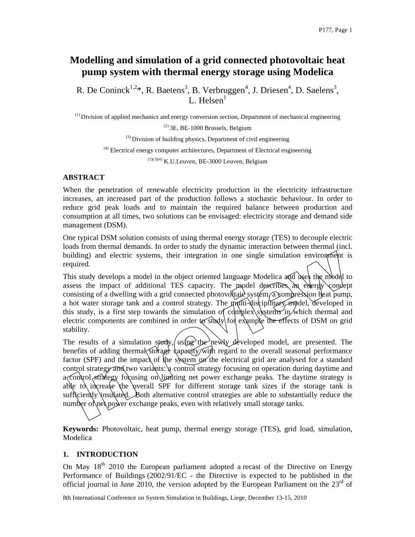
The model is schematically presented in Figure 1. It consists of a 2-zone building, an air-to-water heat pump, a stratified storage tank, a heat distribution system with two radiator circuits

P177,


and a grid connected PV system. The different components of the model are described in sections 2.1 to 2.4.

Figure 1 – General model scheme

2.1 Building

In this paper, a high-order lumped capacitance model (Clarke 2001, Underwood & Yik 2004) for predicting the unsteady building response is developed within Modelica. A first-order lumped capacitance approach is used for each of the different construction layers of the building, whereas a second-order model is used for all surface layers in order to cope with restrictions for low Biot-numbers (Incropera et al. 2007) and to allow a more accurate prediction of indoor surface temperatures. Similarly as in the TRNSYS type56, inter-surface longwave radiation is modeled by means of a zone star temperature (Davies 1993), reducing the complexity of the model compared to view factors and allowing a straight-forward implementation of internal convective and radiative gains.

The absorption, transmission and reflection of solar radiation through the array of air and glass layers in the windows is modeled with the embedded technique described by Edwards (1977, 1982). The transmitted diffuse short-wave solar radiation is distributed over all room surfaces weighted to their surface and absorption coefficient, whereas the direct short-wave solar gains are modeled to fall on the floor. Liesen & Pedersen (1997) show that only small differences would arise when making different assumptions on the distribution of the transmitted solar energy.

Within the developed building model, a stochastic generated occupancy profile from Richardson et al. (2008) and domestic load profile are included. The modeled domestic electricity consumption profile takes into account standby power (de Almeida et al. 2008) and domestic cooling appliances (Firth et al. 2008, Liu et al. 2004), lighting (Stokes et al. 2004, Richardson et al. 2009), fan operation, cooking (Glorieux & Vandeweyer 2002, Wood & Newborough 2003) and the use of media like television and computer (Glorieux &

P177,


Vandeweyer 2002, TPDCB 2010). For the purpose of detailed energy prediction and simulation, the original tool for lighting has been coupled to minute global irradiance data derived from Meteonorm 6.1 (Meteotest, 2008) for Uccle, Belgium. The use of the washing machine and tumble dryer are not modelled in detail as their current use is determined by the day and night regime of electricity resulting in a lack of relevant information on their usage and consumption profiles.

The modelled building is conceived as an energy regulation complying building with two rectangular thermal zones (day zone and night zone) with a floor surface of 80 m² each. The walls are massive cavity walls with 15 cm of mineral wool (λ=0.036 W/mK), The roof also contains 15 cm of mineral wool, the floor is insulated with 10 cm PUR. All windows have double glazing (U=1.1 W/m²K). An uncontrolled natural ventilation with fixed air change rate of 0.3 ACH is assumed. All internal gains as well as the occupation hours are based on the stochastic methods described above. The occupation determines the heating set point (21°C in the day zone, 16°C in the night zone), there is no heating outside the occupation hours.

2.2 Heating system

The hydraulic scheme of the heating system is presented in Figure 2. The model is based on the ‘hydronic heating’ example in the Modelica Building library v0.8, developed by Michael Wetter (2009). The heat production system is composed of an air-to-water heat pump (on-off control), a storage tank, supply and return ducts and a pump (P1). The heat distribution side consists of a pump (P2), a three-way valve to control the water temperature, supply and return ducts and two heat emission circuits, each composed of a radiator, a thermostatic valve and two ducts.

Figure 2 – Simplified hydraulic scheme of the heating system, with basic nomenclature

The heat pump characteristics are derived from catalogue data from the Viessmann Vitocal 350 heat pump (Viessmann, 2006). The thermal (QHP) and electric power (PEl,HP) are expressed as a function of ambient temperature and condenser temperature THP, as presented in equations (1) and (2).

+⋅+⋅⋅= 3.13862.8414.26

10000,

, HPAmbQ

P TTnomHPHPEl

(1)

+⋅+⋅⋅= 1098975.24148.1

10000

2,

AmbAmbQ

Q TTnomHPHP

(2)

P177,


In the model developed within this study, the heat pump has an internal water volume and internal dry mass which are coupled to assign an equal temperature. Thermal heat pump losses are modeled between on the one hand this internal volume and dry mass and on the other hand the surroundings (assumed to be constant at 15°C). The instantaneous coefficient of performance (COP) of the heat pump can be calculated as QHP/PEl,HP. Equations (3) and (4) define two different seasonal performance factors (SPF), based on the nomenclature of Figure 2.

∫= ∫

HPEl

HP

pumpheat P

QSPF

,

(3)

∫∫∫∫ ∫

++

+=

2,1,,

2,1,

PElPElHPEl

heatingheating

systemPPP

QQSPF

(4)

The storage tank has ten stratification layers with a uniform temperature each. Heat conduction is modeled between the layers through the fluid, and between the layers and the surroundings (at constant temperature of 15°C). Temperature inversion is detected and the concerned layers are ideally mixed (Wetter, 2009). Two temperature sensors are available in the tank, TTop in the upper layer and TBot, in the 8th layer (2nd but last).

A dynamic radiator model has been implemented. To allow for varying mass flow rates, the transferred heat is computed using a discretization along the water flow path (10 steps), and heat is exchanged between each compartment and a uniform room air and radiation temperature. For the transient response, heat storage is computed using a finite volume approach for the water and the metal mass, which are both assumed to be at the same temperature (Wetter, 2009).

The thermal behavior of the ducts is neglected. The ducts are simulated taking into account only their pressure drop (dp) with a fixed flow coefficient k=mflow/√(dp). Near the origin, the square root relation is linearized to ensure that the derivative is bounded. A linearized flow characteristic is assumed for all valves, the three-way valve has a leak flow rate of 1% of the nominal flow rate. The pumps have a (linear) flow characteristic that defines the relation between flow rate and pressure drop (Wetter, 2009).

Pump P2 (Figure 2) is pressure drop controlled: it keeps a predefined pressure drop between its inlet and outlet at all times. The thermostatic valves are temperature controlled. A temperature setpoint (operative temperature) is received from the building model, based on occupancy. A proportional controller converts the difference between the setpoint and actual operative temperature in a control signal between 0 and 1 that is passed to the thermostatic valve.

2.3 Photovoltaic system

The PV panels are modeled using the single-diode equivalent circuit. This consists of a current source, Iph, a Diode with current Io, a shunt resistor Rsh and a series resistor Rs. Here Iph represents the light current and Io the diode reverse saturation current. The equation of this equivalent circuit is given by (5), with i representing the current flowing out of the panel and v the voltage at the clamps.

P177,


s

s t

v iRn V s

ophsh

v iRi I I e

R

+

+= − −

(5)

The five parameters in this model, Iph, Io, Rsh, Rs and Vt are calculated following the method described by Sera, Teodorescu, and Rodriguez (2007). The parameters are calculated based on characteristics of the PV panel which are, in most cases, provided by the manufacturer. These specifications are the current Impp and voltage Vmpp at the maximum power point under standard testing conditions (STC), the short circuit current Isc and open circuit voltage Voc at STC, and the temperature coefficients ki and kv of the short circuit current and open circuit voltage. Given Vmpp and Impp should satisfy equation (5), the derivative of the power with respect to the voltage at maximum power point should be zero and the derivative of the current with respect to the voltage at short-circuit current should be the negative of the shunt conductance, Rs, Rsh and Vt can be calculated. Io and Iph at STC can be found from equation (5) for the short-circuit and open-circuit condition.

In this study, 30 panels, all considered to be identical, with 230 Wp each are modeled. The output per PV panel is calculated given perfect maximum power point tracking capability. This output is assumed to be dependent on the position of the sun, the radiation and the ambient temperature.

The position of the sun is given by minute values of the zenith angle from the meteoreader and the orientation is calculated using the time of the day. The sun’s position together with the orientation and tilt of the PV panels, gives the incidence angle of direct beam radiation on the panel and allows to calculate the amount of beam radiation that gets reflected and passes the PV panel cover using incidence angles modifiers derived from De Soto, Klein, and Beckman (2006).

The absorbed solar radiation is calculated given the incidence angle modifiers and minute values for the diffuse and direct beam radiation supplied by the meteoreader, together with the ground reflected radiation (De Soto et al. 2006). The ambient temperature, together with the temperature rise caused by the absorbed radiation and the panel efficiency, enable to estimate the cell temperature. Cell temperature and absorbed radiation are used to calculate the parameters of the PV panel for non-reference working conditions (De Soto et al. 2006). Solving equation (5) for these new parameters and given the assumption of perfect maximum power point tracking capability and constant inverter efficiency yields the electrical energy output of the PV system.

2.4 Heat pump control

A heating curve is defined, through which the heating curve temperature (Thc) is calculated as follows (Wetter, 2009):

lR

NRNSmlR

NRNSRhc QT

TTQT

TTTT Re

,,Re

,,

22

1

⋅

−−

+⋅

−+

+=−

(6)

In this equation, TR is the room temperature, TS,N and TR,N are the nominal supply and return temperature and QRel is the relative heat demand calculated as:

DesignR

AmbientRl TT

TTQ

−−=Re

(7)

with TDesign the minimum outdoor temperature for which the heating system is designed.

P177,


This heating curve incorporates the heat emission characteristics of the radiators by taking into account the heat transfer exponent m. In most heating systems, the heating water temperature set point (HWTS) is a running average of the heating curve temperature with a time lag typically between four and twelve hours. However, as shown in Figure 3, such a HWTS is still relatively sensitive to intra-day temperature variations.

Another approach would be to apply a first order filter to the heating curve in order to flatten out the intra-day oscillations. The effect of a first order filter with a time constant of twelve hours is presented in Figure 3, showing that a filtered HWTS is more dampened.

Optimization of the HWTS is not the subject of the present study. All simulations are made with a first order filter with a time constant of twelve hours on the set point.

Figure 3 – HTWS without modifier (= Thc), as running average with twelve hours time lag and filtered

with twelve hours time constant for two weeks. Thc is calculated based on TR =20°C, TS,N =60°C, TR,N =50°C and TDesign=-8°C

The heat pump control strategy is based on comparing the top and bottom tank temperatures (TTop and TBot) with the current HWTS as shown in equations (8) and (9).

KHWTSTTopwhenHPon 3+< (8)

KHWTSTBotwhenHPoff 4+> (9)

The HWTS has not only a large impact on the COP of the heat pump, it also influences to some extent the operation time of the heat pump when a storage tank is present. This is shown in equation (8): when the HWTS is rising, HPon will become true and the heat pump has to start.

In systems with a small storage tank, the heat pump has to follow the heat demand closely. Therefore we can say that the heat pump operation is largely determined by the heat demand and the time derivative of the HWTS, whereas the heat pump’s COP is mainly determined by the HWTS and the ambient temperature.

Three different control strategies have been analysed in this work:

1. Heating Curve – control of the heat pump solely based on the equations (8) and (9);

P177,


2. Daytime – satisfaction of equation (8) + additionally trying to charge the storage tank during a predefined daytime period;

3. Grid load - satisfaction of equation (8) + additionally starting AND shutting down the heat pump when the net power exchange exceeds predefined boundary values;

The details of these control strategies are explained in their respective sections in the next chapter.

3. SIMULATION RESULTS AND DISCUSSION

3.1 Modelica simulation

The simulations are all carried out over a period of 6 weeks, starting at the 1st of January, thereby focusing on heating during the winter season. The meteodata are minute values for solar radiation and ambient temperature computed by Meteonorm 6.1 (Meteotest, 2008) for Uccle, Belgium. The solar irradiation on the building and PV surfaces are computed with a radiation processor TRNSYS 16 and imported in Modelica.

All simulations are performed with Dymola 7.3. For information, the simulation duration for 6 weeks ranged from 1h to 2h (depending on the computer used) with 4th and 5th order stiff solvers esdirk34a and esdirk45a.

3.2 Reference situation

The reference situation has a storage tank with a volume of 300 l and a thermal resistance of the insulation of 2.5 m²K/W. The averaged (over six weeks) heat demand of the building as a function of the hour of the day is presented in Figure 4, which shows that the majority of the heat demand occurs in the morning with a second, much smaller peak towards the evening. However, similar to all user behavior, the heat demand is stochastically computed and therefore this average demand cannot be seen as a profile.

A sequence (time series) of temperatures for 4 days is presented in Figure 5. This figure shows the stochastic nature of the operative room temperatures, and consequently the heat demand, and the occurrence of short occupancy periods. In average over the six simulated weeks, there are two occupancy periods per day. To check the thermal comfort, all hours for which the operative temperature of one of the rooms is 1K below the setpoint are summed. For all simulations discussed in this paper, the number of thermal discomfort hours is in the range [57h – 63h].

Taking into account thermal losses from the heat pump to the surroundings, the heat pump SPF, as defined in equation (3) is 2.41 for the reference situation. The heating system SPF, defined in equation (4) reaches 2.29.

P177,


Figure 4 – Average ambient temperature (top) and heat demand (bottom) by hour of the day over six

weeks. The figure also shows the averaged HWTS (top) and the averaged nominal COP of the heat pump (bottom)

Figure 5 – Time series of ambient temperature and room temperatures (top) and HWTS and storage tank

temperatures (bottom) for four typical days

P177,


3.3 Heating curve control strategy

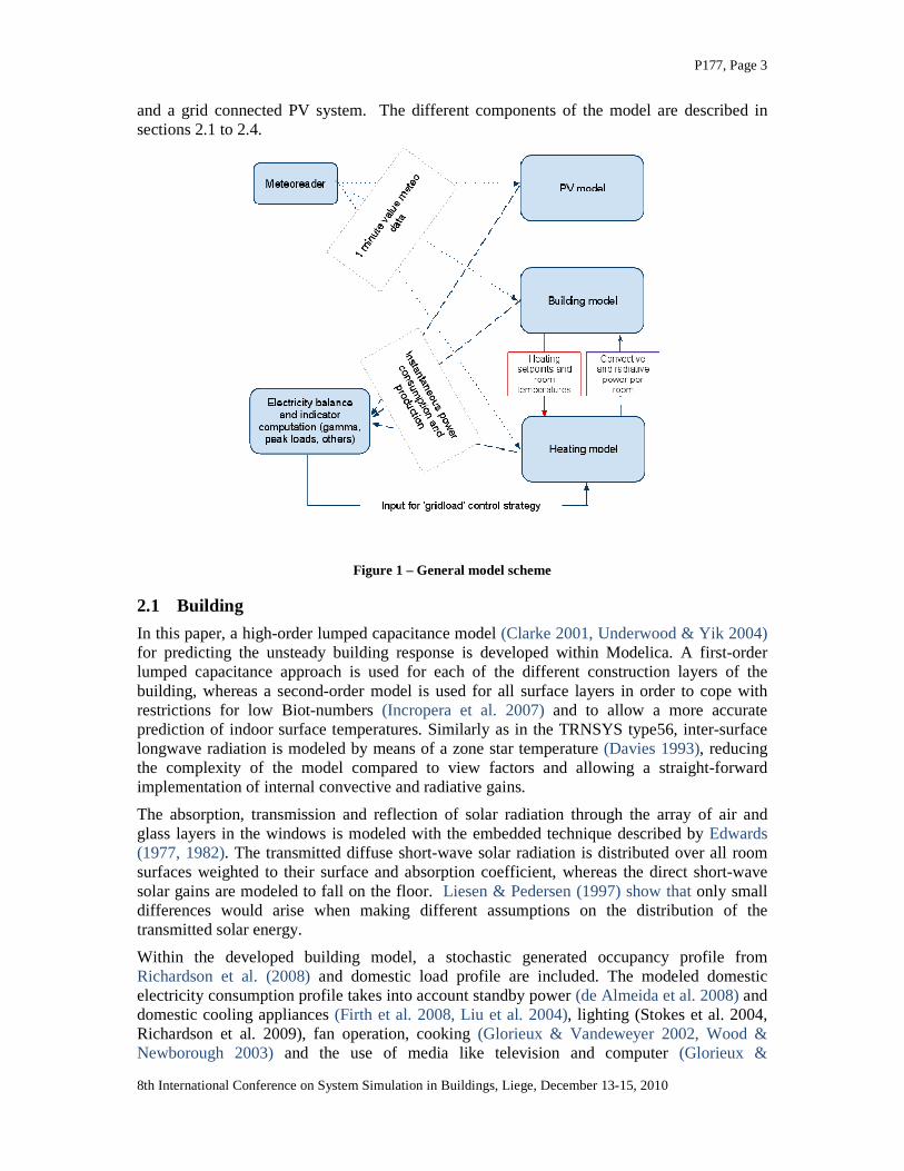
In a first series of simulations, the effect of increasing the storage tank size is analysed without changing the control strategy. Figure 6 shows the evolution of heat pump and heating system SPF with the storage size. It is clear that the total system efficiency is always lower than the reference case, due to the additional thermal losses of the storage tank, even for higher heat pump efficiencies (in some cases). The average distribution of the heat pump power as a function of the hour of the day is shown in Figure 7 for different storage volumes.

Figure 6 –SPF of heat pump (grey triangles) and total heating system (black dots) for the heating curve

control strategy as a function of storage size, compared to the reference case (= 300 l storage tank)

Figure 7 – Average distribution of heat demand and heat pump power as a function of the hour of the day

for the heating curve control strategy

It is clear that the matching between the average heat demand and the average heat pump power reduces with increasing storage volume. For a single dwelling this is not very important, but when different buildings with heat pumps are clustered, flattening out of the heat pump operation times will have a large impact on the cluster’s peak power and capacity factor.

P177,


3.4 Daytime control strategy

The second control strategy aims at increasing the heat pump’s SPF by shifting its average operation time. As seen in Figure 4, operating the heat pump in the afternoon would lead to higher SPF’s thanks to the higher ambient temperature (on average).

There are different solutions to implement such a control strategy. One option, Model Predictive Control (MPC), tries to optimize the control by using a simulation based forecast of the boundary conditions and state variables (Bianchi, 2006). This approach is for instance applied by Degrauwe et al. (2010) for similar air-to-water heat pumps as used in the current study.

In the current research, we have deliberately chosen for a simple control strategy based on very few real-time measurements. The aim is to study the impact of some variations rather than optimizing the control strategy.

As in the heating curve control, the daytime control will always satisfy equation (8). Based on Figure 4, the daytime period (DTP) is fixed from 12 AM till 7 PM. During this period, the storage tank is charged until it is completely full (equation (9)), outside this period, charging stops when the tank top temperature is again at HWTS + 3K. However, a minimum on-time of 20 minutes for the heat pump is implemented.

In order to increase the probability of charging during DTP, the controller will not wait until equation (8) is met. Therefore, a tank state of charge (SOC) is defined that enables to assess the charge status at any time. When the SOC is below a pre-defined threshold during DTP, charging will start. Even though the tank has 10 nodes, with regard to practical implementation, the SOC is defined based on two temperature measurements only, in the top and 8th layer of the tank (see Figure 2).

The definition is based on the principle that two partial SOC values are determined, one for each temperature sensor, and the tank SOC is computed as the average of those two partial values.

2BotTop

Tank

SOCSOCSOC

+=

(10)

The values for the partial states of charge are determined by linear interpolation between a value for SOC=0 and SOC=1, as illustrated in Figure 8.

SOCTop

T

1

HWTS+ 3K

HWTS + DTHP,Nom

SOC

0

SOCTop

T

1

HWTS+ 3K

HWTS + DTHP,Nom

SOC

0

SOC

T

0

1

HWTS –DTHeat,Nom

HWTS + 4K

SOCBot

SOC

T

0

1

HWTS –DTHeat,Nom

HWTS + 4K

SOCBot

Figure 8 – Principle used to determine the partial SOCTop (left) and SOCBot (right)

In order to determine the required four boundary conditions for SOCTop and SOCBot the following reasoning is applied. The tank is completely empty (SOCTank=0) when equation (8) is met. This defines the TTop for condition SOCTop=0. At that time, it is assumed that TBot

P177,


is at the heating system’s return temperature, HWTS-DTHeating, nom, with DTHeating, nom the nominal temperature difference between heating supply and return. This results in the condition for SOCBot=0.

On the other hand, the tank is completely full (SOCTank=1) when equation (9) is met. This defines the TBot for condition SOCBot=1. In order to determine the condition for SOCTop=1, it is assumed that when equation (9) is met, the real bottom temperature in the tank (10th node) is equal to HWTS. The assumed TTop at that time is then HWTS + DTHP, nom, with DTHP, nom the nominal temperature difference between condenser in- and outlet.

This definition of SOC is used in both the daytime and grid load control strategies with DTHeating, nom = 15 K and DTHP, nom = 14 K. It can be noted that SOCTank is completely depending on HWTS, and therefore it is a unit-free indicator of the energy content of the storage tank with respect to the current heating needs, not compared to the surroundings.

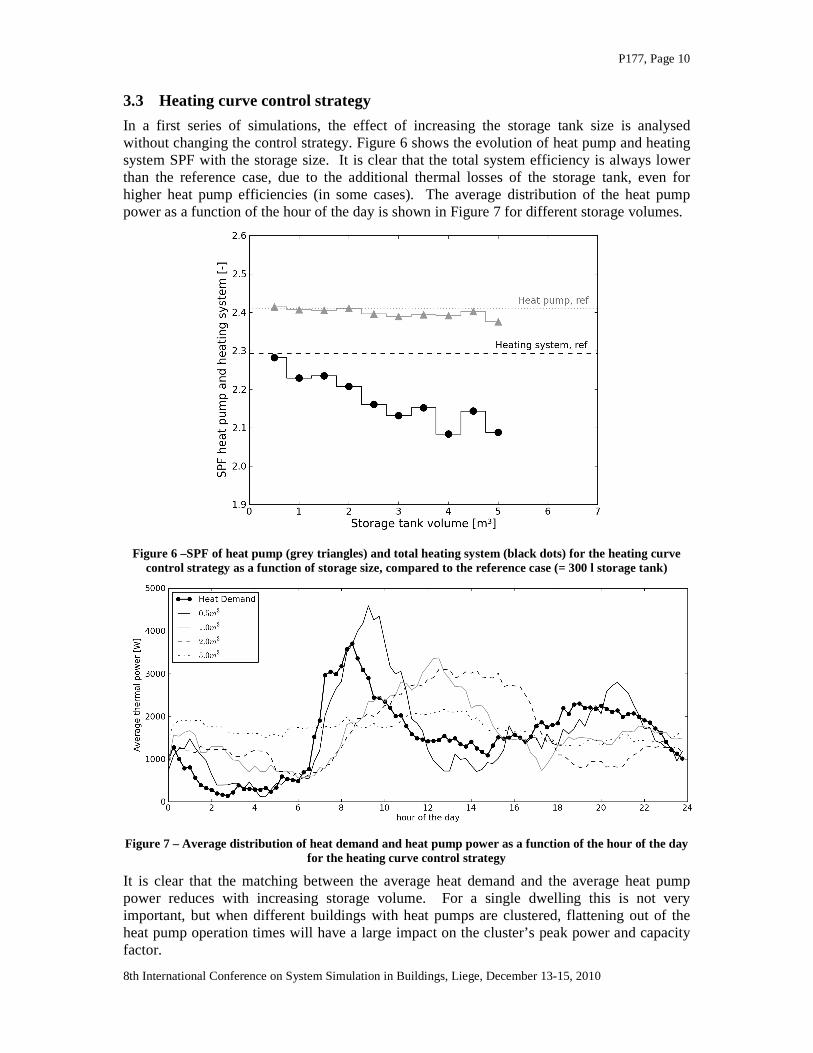
The averaged thermal heat pump power as a function of the hour of the day is presented in Figure 9 for different storage sizes when the daytime control strategy is applied. The DTP can be clearly identified on this graph, and it can be seen that for all storage sizes, the heat pump operates most often during DTP. However, in the case of small tanks, the heat pump has to shut down much before the end of the DTP because the tank is full. As a consequence, for these small tank volumes, the heat pump has to run more often beyond the DTP, especially in the morning when the heat demand is large. From 1 m³ tank volume upwards, it is possible to produce most of the heat during DTP.

Figure 9 - Average distribution of heat demand and heat pump power as a function of the hour of the day

for different storage sizes, using the daytime control strategy

Figure 10 shows that the daytime control strategy is able to raise both the heat pump and system SPF, but only for a small storage tank of 0.5 m³. Due to increasing storage losses, the system SPF drops quickly with increasing tank volume.. Additional simulations have been performed with a better insulation of the tank (5 and 10 m²K/W respectively). The resulting system SPF’s are shown in Figure 11. These results show clearly that insulation of the storage tank is a crucial parameter. This conclusion is not new in the context of air-to-water heat pumps, it agrees with measurements performed by Verhelst et al. (2008). With well insulated tanks, it is possible to increase the system SPF with up to 4% compared to the reference situation.

P177,


Figure 10 –SPF of heat pump (grey triangles) and total heating system (black dots) for the daytime control

strategy as a function of storage size, compared to the reference case

Figure 11 –SPF of total heating system, daytime control strategy, as a function of storage size, compared

to the reference case. Three different insulation levels, from lower to higher: 2.5, 5 and 10 m²K/W

3.5 Grid load control strategy

When different buildings with identical or similar energy concepts are connected to the same electricity grid, the simultaneity of the electricity demand and injection peaks can cause the grid to collapse. Therefore, a third control strategy is implemented that tries to reduce peaks, both positive (consumption) and negative (injection).

The principle of the grid load control strategy is to try to keep the storage tank at an intermediate SOC at all times in order to be able to switch off or on the heat pump when the power consumption respective injection surpasses a predefined threshold, identified as BCons and BInj.

When the net power exchange Pg reaches the threshold (either BCons or BInj), switching on or off the heat pump (on when Pg<BInj, off when Pg>BCons) will always lower the net power exchange (if the total threshold band, BCons - BInj is larger than the heat pump power PHP

P177,


which is always the case in this study). Defining the switching on condition when there is no immediate emergency is more difficult because the electric power consumption of the heat pump is variable and thus the resulting net power exchange after switching on can not be known in advance.

To cope with this issue, the electricity consumption of the heat pump immediately after switching on (PHp,last) is stored in the internal memory of the controller and the resulting conditions for switching on the heat pump are given by equation (11).

( )

)4(

))((

3

,

Injg

lastHPConsgStartTank

on

BPANDKHWTSTBotOR

PBPANDSOCSOCOR

KHWTSTTopwhenHP

>+<

−<<+<

(11)

The conditions for switching off the heat pump are given by equation (12):

( )[

])4(

)(

))((

)3(min20

KHWTSTBotOR

BPOR

PBPANDSOCSOC

ANDKHWTSTTopnotANDtwhenHP

Consg

HPInjgStopTank

onHPoff

+>

>

+>>

+<>

(12)

These equations contain different parameters; in the following simulations SOCStart is always 0.5, SOCStop is 0.7 and the absolute value of BInj and BCons is either 3500 or 4500W.

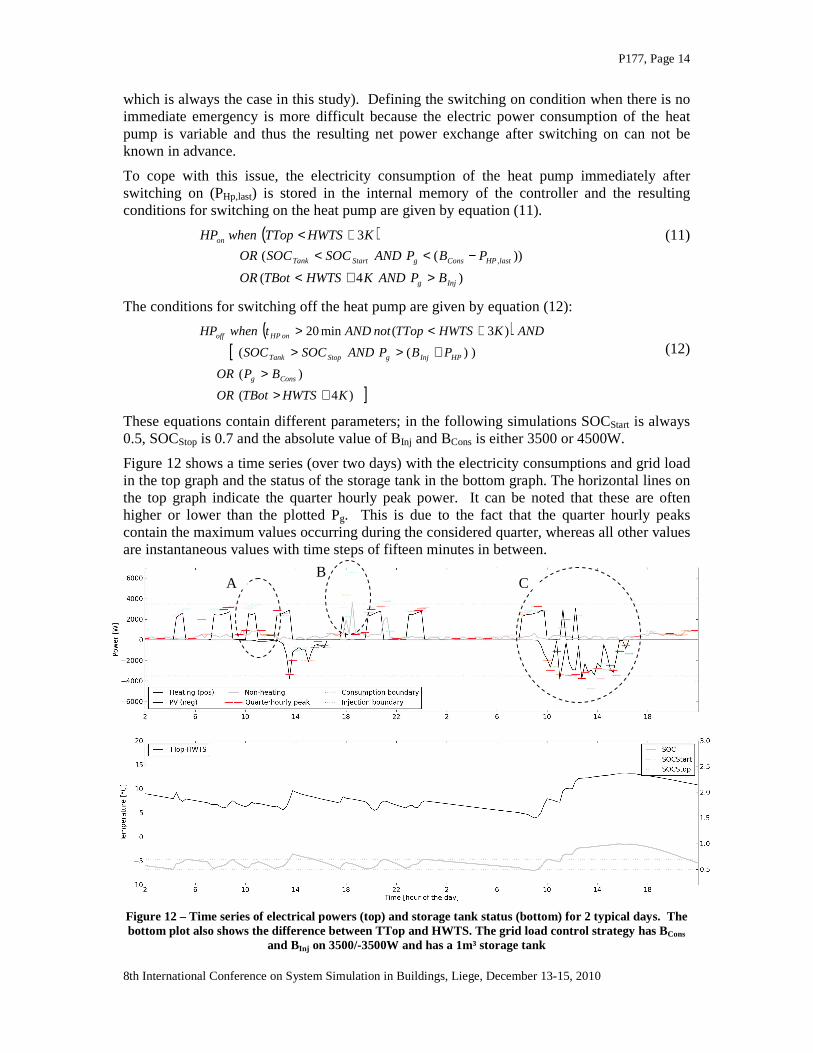
Figure 12 shows a time series (over two days) with the electricity consumptions and grid load in the top graph and the status of the storage tank in the bottom graph. The horizontal lines on the top graph indicate the quarter hourly peak power. It can be noted that these are often higher or lower than the plotted Pg. This is due to the fact that the quarter hourly peaks contain the maximum values occurring during the considered quarter, whereas all other values are instantaneous values with time steps of fifteen minutes in between.

Figure 12 – Time series of electrical powers (top) and storage tank status (bottom) for 2 typical days. The bottom plot also shows the difference between TTop and HWTS. The grid load control strategy has BCons

and BInj on 3500/-3500W and has a 1m³ storage tank

B A C

P177,


Figure 12 illustrates some interesting phenomena:

A. the heat pump is shut down, otherwise Pg would become larger than BCons ;

B. the heat pump is shut down, but this is not enough to limit Pg and 2 (quarter hourly) peaks appear. The first one is occurring during operation of the heat pump, since the heat pump cannot immediately shut down because of the requirement to operate minimum 20 minutes. The second peak is due to the non-heating electricity consumption only;

C. in order to limit power injection to 3500 W, the heat pump starts to charge the storage tank above a SOC of 0.7, but has to stop when TBot reaches HWTS+4K. With a larger tank (or a lower initial SOC), the following peaks could probably have been avoided.

3.6 Grid impact

To assess the degree of success of the studied control strategies, objective indicators need to be defined. In the discipline of electrical engineering, the capacity factor (CF, defined as the peak power/rated connection (kW/kVA)) and full load equivalent hours (FLEHO, defined as yearly consumption/peak power, in h) are often used. These indicators contain no information, however, on the amount of peaks that occur. Moreover, the FLEHO will improve when the consumption increases for a given peak power, making it even less suited to compare control strategies.

In the current study the indicators that have been chosen are the one percent peak (OPP) and the percentage of time with a net grid exchange above 5000 W (both injection and consumption). The OPP is defined as the mean power of the one percent highest quarter hourly peaks. The 5000 W barrier has been chosen since this is a point at which some grid connections might change, i.e. PV systems of more than 5000 Wp should have a three phase connection. The combination of these indicators gives an idea of the value of the highest peaks and the amount of peaks.

A histogram of the quarter hourly peaks is shown in Figure 13 for the reference and the two alternative control strategies. The histogram shows that the majority of quarter hourly peaks is situated between 0 - 1000 W, with a second group of peaks situated between 2000 - 4000 W.

P177,


Figure 13 – Histogram of quarter hourly peaks. Ordinate corresponding to the x value shows the amount of peaks during the considered 6 week period for which the peak lies between x +/- 50 W. Consumption is

positive. 3 cases are shown: reference, grid load control strategy with both boundaries at -3500 W and 3500 W and 1 m³ storage and daytime control strategy with 1 m³ storage tank. The boundaries are

visualised, as is the 5000 W boundary used as indicator

In the current study the indicators that have been chosen are the one percent peak (OPP) and the percentage of time with a net grid exchange above 5000 W (both injection and consumption). The OPP is defined as the mean power of the one percent highest quarter hourly peaks. The 5000 W barrier has been chosen since this is a point at which some grid connections might change, i.e. PV systems of more than 5000 Wp should have a three phase connection. The combination of these indicators gives an idea of the value of the highest peaks and the amount of peaks.

The impact of the grid load strategy on the two defined indicators is presented in Figure 14. The results show that already with a relatively small storage tank of 0.5 m³ or 1 m³, both the OPP and the number of peaks > 5 kW can be significantly reduced. The number of peaks can be reduced by almost 50% in the best cases, the OPP by around 20%. However, the highest peaks could not be eliminated, they are not caused by the heat pump nor the PV system.

P177,


Figure 14 – Impact of grid load control on OPP and percentage of time > 5 kW for different storage tank volumes. Left plot is with boundaries at 4500 and -4500 W, right plot has boundaries at 3500 and -3500 W.

The impact of the daytime control strategy on the grid indicators is presented in Figure 15. It is clear that the results are very positive for 1 m³ and 1.5 m³ storage tanks. The reason for this low grid impact can be understood by analyzing Figure 16, which shows the average electricity production and consumption (heating and non-heating) as a function of the hour of the day. The graph shows that the heat pump works most often during periods characterized by large PV production, thereby reducing both positive and negative power peaks.

Figure 15 – Impact of daytime control strategy on OPP and percentage of time > 5 kW for different

storage tank volumes

The overall results for a selection of cases are shown in Figure 17. From these results, it can be observed that different control strategies and different settings of those control strategies are able to reduce the grid impact. However, all cases have lower system SPF values than the

P177,


reference. When the results of Figure 11 are kept in mind, one can conclude that with better insulated storage tanks, the daytime strategy is able to save energy compared to the reference case.

Figure 16 - Average distribution of heat demand (thermal) and electric power for heat pump (daytime

control strategy, 1m³ tank), non-heating consumption and PV production as a function of the hour of the day

Figure 17 – Comparison of different control strategies. OPP and percentage of time > 5 kW (top), SPF (bottom) of heating system (black dots) and heat pump (grey triangles). DT stands for daytime, GLxxxx for grid load with boundaries xxxx.

P177,


4. CONCLUSION

In this study, a dwelling equipped with PV and a heating system based on an air-to-water heat pump has been modeled in Modelica, an open source and object oriented equation based modeling language. The study aimed at investigating the effect of 3 different control strategies (heating curve only, daytime priority and grid load based) on the total efficiency and grid impact of the system.

In order to control the stratified storage tank, a state of charge has been defined based on two temperature measurements in the tank and the current heating water temperature setpoint.

The study has shown that increasing the storage volume will automatically increase the overall energy consumption (and thus decrease the system performance factor) unless an adapted control strategy is applied. With a daytime priority control strategy and a well insulated tank, energy savings are possible, although they are relatively small (4%). This result emphasizes the importance of careful insulation of storage tanks.

In order to reduce the impact on the grid, the grid load control strategy was implemented. The strategy works well and is able to reduce the amount of peaks by almost 50%. The remaining peaks are mainly caused by the non-heating electricity profile. Therefore, the combination of a storage tank of only 1 m³ and an adapted control strategy is able to eliminate almost completely the consumption peaks caused by users and the heating system. The effectiveness of reducing injection peaks largely depends on the size of the storage tank.

It is noteworthy that the daytime strategy, which is clearly less complicated and does not require power meters, can reach the same effect on the grid impact if the heat pump operation time is prioritized during periods when the PV system is likely to reach high power outputs.

If the capacity factor is to be reduced, which means lowering the highest peak, a more global DSM strategy will be required because the highest peaks in the current model are not caused by the heating or PV system.

This study clearly has its limits, one of the major being the fact that simulations were only carried out over a 6 weeks winter period. The next steps consist of extending the simulations to a whole year, improving the building design in order to reach lower energy demands, and studying the potential impact of storage on the nominal power of the heat pump.

5. ACKNOWLEDGEMENTS

The authors gratefully acknowledge the K.U.Leuven Energy Institute (EI) for funding this research through granting the project entitled Optimized energy networks for buildings.

6. REFERENCES

Åkesson, J., Årzén, K., Gäfvert, M., Bergdahl, T., & Tummescheit, H. (2009). Modeling and optimization with Optimica and JModelica.org—Languages and tools for solving large-scale dynamic optimization problems. Computers & Chemical Engineering. doi: 10.1016/j.compchemeng.2009.11.011.

Baetens, R., De Coninck, R., Helsen, L., Saelens, D. (2010). The impact of domestic load profiles on the grid-interaction of building integrated photovoltaic (BIPV) systems in extremely low-energy dwellings, Presented at ‘The renewable energy research conference (RERC)’, June 06, 2010, Trondheim, Norway

Bianchi, M. A. (2006): Adaptive Modellbasierte Prädiktive Regelung einer Kleinwärmepumpenanlage, PhD Thesis, ETH Zürich.

P177,


Clarke, J.A. (2001). Energy simulation in building design (2nd ed.). Oxford: Butterworth-Heinemann.

Davies, M.G. (1993). Definitions of room temperature. Building and Environment 28, 3838-398.

de Almeida, A., Fonseca, P., Bandairinha, R., Fernandes, T., Araújo, R., Nunes, U., Dupret, M., Zimmermann, J.P., Schlomann, B., Gruber, E., Kofod, C., Feildberg, N., Grinden, B., Simeonov, K., Vorizek, T., Markogianis, G., Giakoymi, A., Lazar, I., Ticuta, C., Lima, P., Angioletti, R., Larsonneur, P., Dukhan, S., de Groote, S., de Smet, J., Vorsatz, D., Kiss, B., Loftus, A.-C., Pagliano, L., Roscetti, A. & Valery, D. (2008). REMODECE - Residential monitoring to decrease energy use and carbon emissions in Europe. Final report, p.96.

De Soto, W., Klein, S. A., & Beckman, W. A. (2006). Improvement and validation of a model for photovoltaic array performance. Solar Energy, 80, 78-88. doi: 10.1016/j.solener.2005.06.010.

Degrauwe, D., Verhelst, C., Logist, F., Van Impe, J. & Helsen, L. (2010). Multi-objective optimal control of an air-to-water heat pump for residential heating. In SSB2010 (pp. 1-14).

Edwards, D.K. (1977). Solar absorption by each element in an absorber-coverglass array. Solar Energy 19, 401-402.

Edwards, D.K. (1982). Finite element embedding with optical interference. International Journal of Heat and Mass Transfer 25, 815-821.

EurObserv'ER (2009). Baromètre photovoltaïque / Photovoltaic barometer : 9 533,3 MWc dansl'UE / in the EU. Systèmes solaires - Le journal du photovoltaïque 1, 72-103.

European Heat Pump Association. (2010). Outlook 2010 European Heat Pump Statistics - Summary. Brussels. Retrieved from www.ehpa.org (last consulted on July 16, 2010).

Firth, S., Lomas, K., Wright, A. & Wall, R. (2008). Identifying trends in the use of domestic appliances from household electricity consumption measurements. Energy and Buildings 40, 926-936.

Glorieux, I. & Vandeweyer, J. (2002). Statistische studie nr110 - 24 uur ... Belgische tijd, een onderzoek naar de tijdsbesteding van de Belgen.

Houseman, D. (2009). True Integration Challenges For Distributed Resources In The Distribution Grid. In 20 th International Conference on Electricity Distribution 20 th International Conference on Electricity Distribution Prague , 8-11 June 2009 (p. Paper 0012). CIRED.

Incropera, F.P., and DeWitt, D.P., 2002. Fundamentals of Heat and Mass Transfer. 5th ed. John Wiley & Sons, Hoboken, NJ.

Incropera, F.P., DeWitt, D.P., Bergman, T.L. & Lavine, A.S. (2007). Introduction to Heat Transfer (5th ed.). John Wiley & Sons.

Liesen, R.J. & Pedersen, C.O. (1997). An evaluation of inside surface heat balance models for cooling load calculations. ASHRAE Transactions 103, 485-502.

Liu, D., Chang, W.R. & Lin, J.Y. (2004). Performance comparison with effect of door opening on variable and fixed frequency refrigerators/freezers. Applied Thermal Engineering 24, 2281-2292.

Meteotest, 2008. METEONORM Version 6.1 - Edition 2009.

P177,


Pepermans, G., Driesen, J., Haeseldonckx, D., Belmans, R., & D, W. (2005). Distributed generation : definition , benefits and issues $. Energy Policy, 33, 787-798. doi: 10.1016/j.enpol.2003.10.004.

Richardson, I., Thomson, M. & Infield, D. (2008). A high-resolution domestic building occupancy model for energy demand simulations. Energy and Buildings 40, 1560-1566.

Richardson, I., Thomson, M., Infield, D. & Delahunty, A. (2009). Domestic lighting: A high-resolution energy demand model. Energy and Buildings 41, 781-789.

Sera, D., Teodorescu, R., & Rodriguez, P. (2007). PV panel model based on datasheet values. IEEE, (4), 2392-2396.

The European Parliament. (2009). P6_TA(2009)0278 - Energy performance of buildings ( recast ) - (COM(2008)0780). Energy. Retrieved from http://www.europarl.europa.eu/sides/getDoc.do?pubRef=-//EP//NONSGML+TA+P6-TA-2009-0278+0+DOC+PDF+V0//EN (last consulted on May 28, 2010).

The Modelica Association. (1997). Modelica — A unified object-oriented language for physical systems modeling. Simulation Practice and Theory, 5(6), p32. doi: 10.1016/S0928-4869(97)84257-7.

Torcellini, P., Pless, S., Deru, M., & Crawley, D. (2006). Zero Energy Buildings: A Critical Look at the Definition; Preprint. Retrieved from http://www.osti.gov/bridge/servlets/purl/883663-3U8fQe/ (last consulted on June 02, 2010).

TPDCB, 2010. The power consumption database. Available at: www.tpcdb.com (last consulted on June 25, 2010).

Underwood, C.P. & Yik, F.W.H. (2004). Modelling methods for energy in buildings. Oxford, Blackwell Publishing Ltd.

Verhelst, C., , H. Nolens, K. Schoovaerts, and L. Helsen, "Performance of an air-to-water heat pump system in a low energy residential building: modelling and experimental results", 2008. Presented at the "9th IEA Heat Pump Conference", May. 20-22, 2008, Zürich, Switzerland.

Viessmann. (2006). Vitocal 350, Technical description (p. 11). Zaventem.

Vu Van, T., Woyte, A., Soens, J., Driesen, J., & Belmans, R. (2003). Impacts Of Distributed Generation On Distribution System Power Quality. In 7th International Conference Electrical Power Quality And Utilisation September 17-19, 2003, Cracow, Poland (pp. 585-592).

Wetter, M. (2009). Modelica Library for Building Heating, Ventilation and Air-Conditioning Systems. In The 7th International Modelica Conference (pp. 393-402). The Modelica Association. doi: 10.3384/ecp09430042.

modelling and simulation of a grid connected photovoltaic heat pump system with thermal energy

Documents