modelling and implementation of a vision system for
TRANSCRIPT

Modelling and Implementationof a Vision System
for Embedded Systems
Per Andersson
Licentiate Thesis, 2003
Department of Computer ScienceLund Institute of Technology
Lund University

ISSN 1404-1219
Dissertation 16, 2003
LU-CS-LIC:2003-1
Department of Computer Science
Lund Institute of Technology
Lund University
Box 118
SE-221 00 Lund
Sweden
Email: [email protected]
WWW: http://www.cs.lth.se/home/Per Andersson
c© 2003 Per Andersson

iii

iv

ABSTRACT
Today more and more functionality is included in embedded systems,
resulting in an increased system complexity. Existing design method-
ologies and design tools are not adequate to deal with this increase in
complexity. To overcome these limitations application specific design so-
lutions are more common. In this thesis we presents such solutions for
real-time image processing. This work is part of the WITAS Unmanned
Aerial Vehicle (UAV) project. Within this project we are developing a
prototype UAV.
We introduce Image Processing Data Flow Graph (IP-DFG), a data
flow based computational model that is suitable for modelling complex
image processing algorithms. We also present IPAPI, a run-time system
based on IP-DFG. We use IPAPI for early evaluation of image process-
ing algorithms for the vision subsystem of the WITAS UAV prototype.
This is carried out via co-simulation of IPAPI with the other subsys-
tems, such as the reasoning subsystem and helicopter control subsys-
tem. We also show how IPAPI can be used as a framework to derive an
optimised implementation for the on-board system.
FPGAs can be used to accelerate the image processing operations.
Time multiplexed FPGAs (TMFPGAs) have shown potential in both re-
ducing the price of FPGAs and in hiding the reconfiguration time for dy-
namically reconfigured FPGAs. To use a TMFPGA, the operation must
be temporally partitioned. We present an algorithm that does temporal
partitioning on a technology mapped net-list. This makes it possible to
use excising design tools when developing for TMFPGAs.

vi

ACKNOWLEDGEMENTS
I would like to thank my supervisor Krzysztof Kuchcinsky for his sup-
port and help with my work, especially for the advises and help with
the writing of this thesis. I would also like to thank Klas Nordberg and
Johan Wiklund, both from the ISY department of Linkoping university,
for sharing their knowledge in the area of image processing. Without
your help my work would have been much harder.
This work has been carried out at the computer departments at Lin-
koping University and at Lund University. I would like to tank the
staff at both departments for creating a inspiring and relaxed working
environment. A special thank to Flavius Gruian for the help with LATEX
and comments on the writing of this thesis.
I would also like to thank my mother and late father for always
wanting the best for me. My gratitude also go to my sister, her husband
and their soon to be born child, it has always been a pleasure visiting
you.
This work is part of the WITAS UAV project and was supported by
the Wallenberg foundation.

viii

CONTENTS
1 Introduction 1
1.1 Motivation . . . . . . . . . . . . . . . . . . . . . . . . . . . . 1
1.2 Contributions . . . . . . . . . . . . . . . . . . . . . . . . . . 3
2 Background 5
2.1 Embedded System Design . . . . . . . . . . . . . . . . . . . 5
2.2 Image Processing Algorithm Development . . . . . . . . . . 7
2.3 Improving the Design Process . . . . . . . . . . . . . . . . . 8
3 Computational Models 11
3.1 Data Flow Graphs . . . . . . . . . . . . . . . . . . . . . . . . 11
3.1.1 Firing Rules . . . . . . . . . . . . . . . . . . . . . . . 12
3.1.2 Deterministic Behaviour . . . . . . . . . . . . . . . . 13
3.1.3 Consistency . . . . . . . . . . . . . . . . . . . . . . . 15
3.1.4 Recursion . . . . . . . . . . . . . . . . . . . . . . . . . 16
3.2 Analysis of DFGs . . . . . . . . . . . . . . . . . . . . . . . . 18
3.2.1 Consistency . . . . . . . . . . . . . . . . . . . . . . . 18
3.2.2 Static DFGs . . . . . . . . . . . . . . . . . . . . . . . 19
3.2.3 Boolean DFGs . . . . . . . . . . . . . . . . . . . . . . 20
3.2.4 Problems with current DFG variants . . . . . . . . . 20
4 Image Processing-Data Flow Graph 23
4.1 The WITAS Project . . . . . . . . . . . . . . . . . . . . . . . 23
4.1.1 IPAPI - a run-time system for image processing . . 25
4.2 IP-DFG - a computational model . . . . . . . . . . . . . . . 26

x CONTENTS
4.2.1 Hierarchy . . . . . . . . . . . . . . . . . . . . . . . . 27
4.2.2 Iteration . . . . . . . . . . . . . . . . . . . . . . . . . 30
4.2.3 Token mapping functions . . . . . . . . . . . . . . . 33
5 IPAPI 35
5.1 The Architecture of IPAPI . . . . . . . . . . . . . . . . . . . 35
5.2 The AltiVec Implementation . . . . . . . . . . . . . . . . . . 36
5.2.1 The AltiVec Unit in Combination With JNI . . . . . 37
5.2.2 Experimental Results . . . . . . . . . . . . . . . . . . 38
6 Partitioning for Time Multiplexing 41
6.1 Time Multiplexed FPGAs . . . . . . . . . . . . . . . . . . . 41
6.2 The Partitioning Problem . . . . . . . . . . . . . . . . . . . 43
6.2.1 Data Dependency . . . . . . . . . . . . . . . . . . . . 45
6.2.2 Dependency Loops . . . . . . . . . . . . . . . . . . . 46
6.3 The Partitioning Algorithm . . . . . . . . . . . . . . . . . . 49
6.3.1 Scheduling . . . . . . . . . . . . . . . . . . . . . . . . 49
6.3.2 The Priority Function . . . . . . . . . . . . . . . . . . 51
6.3.3 Deadline Inheritance . . . . . . . . . . . . . . . . . . 53
6.3.4 The Size of the Partitions . . . . . . . . . . . . . . . 54
6.3.5 Experimental results . . . . . . . . . . . . . . . . . . 55
7 Conclusions 57
7.1 Summary . . . . . . . . . . . . . . . . . . . . . . . . . . . . . 57

CHAPTER 1
INTRODUCTION
This thesis addresses embedded system design and particularly with
questions related to design of vision systems for Unmanned Aerial Ve-
hicles (UAVs). The focus is on systems dedicated for complex image
precessing. We present contributions in several parts of the design
process of such systems. This thesis presents a computational model
suitable for complex image processing algorithms, a framework based
on this computational model which supports the engineers when de-
riving an optimised implementation and an algorithm for automating
design when targeting time multiplexed FPGAs. The thesis addresses
tool support and design automation, rather than design methodology.
1.1 Motivation
An embedded system is a system dedicated for a particular application,
as opposed to a general purpose system that is designed to run almost
any application. Since an embedded system is designed for a particular
application, it can be tailored for this application, resulting in a system
more suitable for the task compared to a general system. For example
a system with lower price and lower power consumption.
The design process of embedded systems is attaining an increas-
ing interest. One reason for this is the increasing productivity gap. It
is well known that the manufacturing capacity is expected to increase
faster than the design capacity. This has been the situation for some
years now. There already is a difference in system complexity of what
can be manufactured compared to what can be developed. Increasing

2 Introduction
the development productivity will be the main challenge for researchers
in the near future. One approach to increase the productivity in the de-
sign process is to improve the individual design steps. This includes
better design tools, i.e. faster simulators and more accurate estimators.
With better design tools, a larger part of the design process can be auto-
mated. Decisions can be based on more accurate data, which will lead
to fewer iterations of the design steps. This approach can give a re-
spectable increase in productivity, but it will not give the leap in design
productivity that is needed to solve the productivity gap problem. It
is believed that a leap in productivity can be achieved by allowing the
designer to work on a higher level of abstraction, in a computational
model and language suitable for the application he is currently work-
ing on. The most suitable computational model and language will most
likely be different for different parts of a system. To be able to use this
approach tools that support multiple models of computation are needed.
Those can be tools from different vendors cooperating trough an open
interface.
A consequence of the productivity gap is that the development cost
is an increasing part of the total system cost. One approach to decrease
the development cost of a system is to use platforms. For an application
area a platform is developed and will be used for several products in
that area. The development cost of the platform can be amortised over
a larger number of products and units. The platform is likely to be
more complex than the individual products. To manage this approach
it is important that the developer can manage this complexity. Again
a promising approach to this problem is to work with computational
models and languages suitable for the application. Also it is important
to have design tools that support platforms, encouraging for example
component and architecture reuse.
Time to market is another aspect of embedded system development
that also needs attention. It is important to release a product at the
right time. If it is released to early, the market is not ready or the prod-
uct will be too expensive. If a product is released late it cannot compete
with similar products on the market. This time window can be as short
as a few months. Usually it is more important to be first on the mar-
ket than to have the best product so, in this situation, the development
time reduction is the main challenge for the developers. Increasing the
development productivity can lead to decreased development time, but
there are other approaches too. Development time can be decreased
by increase parallelism in the design process. Hardware/software co-

1.2 Contributions 3
design is one approach which achieves this, co-simulation is another.
The underlying idea is to work on different subsystems in parallel rather
than in sequence. For maximum flexibility, design tools should be open
and able to interact with other tools from different vendors. For exam-
ple, it should be possible to test the implementation of one subsystem
by co-simulation with an abstract model of another subsystem.
To summarise embedded system are becoming more complex as more
functionality is included in these systems. The existing design methods
and tools are not adequate to deal with this increase in complexity. One
promising approach for overcoming the complexity problem is to use
application specific computational models. This requires heterogeneous
designs and, hence, tools supporting this co-design approach. Complex-
ity is not the only problem when designing embedded systems, other
issues, such as time to market, also must be considered.
This thesis attempts to solve some of these problems by introduc-
ing a computational model and a run-time system/simulator for vision
applications.
1.2 Contributions
In this thesis we present our work within the WITAS1 Unmanned Aerial
Vehicle (UAV) project. The work focuses on designing image processing
systems and improving the design process of such systems. Our work
covers a large part of the design process, form the early abstract mod-
elling to generating executables. There are four main contributions:
• The development of a computational model, Image Processing Data
Flow Graph (IP-DFG), tailored for modelling and implementa-
tion of complex image processing algorithms. IP-DFG is based
on boolean data flow graphs which have been extended with hier-
archy and explicit support for iterations.
• Integration of IP-DFG with a run-time system called Image Pro-
cessing Application Program Interface (IPAPI). IPAPI is used in
the WITAS project to co-simulate the vision subsystem with the
other subsystems in the WITAS simulator. IPAPI and the WITAS
simulator is used to evaluate different image processing algorithms.
The original idea of IPAPI comes from Patrick Doherty and Klas
1WITAS is an acronym for the Wallenberg laboratory for research on Information Tech-nology and Autonomous Systems

4 Introduction
Nordberg, both at Linkoping University. We have actively partici-
pated in the development of IPAPI, but the majority of the imple-
mentation of the memory management and scheduling layer has
been done in the computer vision laboratory in ISY, Linkoping
University. Our main contribution is the underlying computa-
tional model and the data processing layer.
• IPAPI evaluation. We show that IPAPI is a good framework for
developing efficient implementations of complex image processing
algorithms. This involves the whole design process, from the early
implementation independent model to the optimised implementa-
tion. We show that by using IPAPI the engineer can focus on the
inner data processing loops and optimise this parts for the target
architecture, while the memory management and scheduling is
automatically managed by IPAPI.
• An algorithm for temporal partitioning. Temporal partitioning is
a new design step needed when using Time Multiplexed FPGAs
(TMFPGAs). The temporal partitioning is fully automated and it
is fast, which makes it suitable for large designs. The method can
be used to implement IP-DFG applications on TMFPGAs.
The rest of this thesis is organised as follows. In chapter 2 we give
our view of embedded systems and we discus the design process for em-
bedded systems. An overview of existing computational models based
on data flow graphs are presented in chapter 3. The computational
model IP-DFG is introduced in chapter 4. In that chapter we also give
a brief overview of the WITAS project. The implementation of IPAPI
and its optimisation for the PowerPC processor is discussed in chapter
5. In chapter 6 the partitioning algorithm for TMFPGAs is described.
Conclusions are presented in chapter 7.

CHAPTER 2
BACKGROUND
In this chapter we discus our view of embedded systems. We discuss
the design process and different ways to improve it. We also relate our
contributions presented in this thesis to the design process.
2.1 Embedded System Design
An embedded system is a system specially designed for a particular ap-
plication. This is different from a general purpose systems that is de-
signed to run any application. Since an embedded system is designed
for a particular application it can be tailored for this application. This
allows more aggressive optimisations and specialisation, resulting in a
system more suitable for the task. This can lead to systems with lower
price and lower power consumption, which is important for mobile ap-
plications.
Over the years, people have proposed different definitions of what
an embedded system is. Instead of giving an exact definition, which is
hard, we give two characteristics that all embedded systems have in
common. An embedded system is a dedicated system and it is of mod-
erate complexity. For example a mobile phone has moderate complexity
and is designed to make phone calls, thus an embedded system. A nu-
clear power plant is a dedicated system, but it is a complex system and
we do not consider it to be an embedded system even though it has sev-
eral characteristics in common with embedded systems. In this thesis
we focus on digital embedded system, that is embedded systems build
from digital components such as CPUs, memories, and ASICs.

6 Background
Since an embedded system is a dedicated system of moderate com-
plexity, people might be mistaken and think that the design of embed-
ded systems is an easy task, the designer is supposed to implement
a specified functionality in a device. However, in reality the situation
is much more complicated. There are many other factors, besides the
functionality, that must be considered. For example, for a mobile phone
the size, price and the standby time are the main selling factors, not
only the ability to use it as a phone. The main problem is finding the
implementation with the best trade-off between the selling factors.
In the beginning of the design process, the functionality of an em-
bedded system can be very abstract, for example to “make a phone call”.
In the early design phases, the behaviour of the embedded system are
made more concrete. This is referred to as behavioural modelling.
The main purpose of the behavioural modelling is to extract prop-
erties, such as computation and memory requirements, to base the ar-
chitecture selection on. During design space exploration, the space of
different architectures is searched for the architecture with the small-
est cost. Here cost does not only mean money, but all beneficial as-
pects, such as power consumption and time to market, can be included
in the cost. During design space exploration the system architecture is
decided, that is which CPUs, ASICs, FPGAs and memory components
will be used and how they are communicating. The functions of the be-
havioural model is mapped to the different components and it is decided
how these components are communicating. (point to point links, busses
or networks)
After the architecture selection, the functionality that was mapped
to the different components needs to be implemented. The implementa-
tions are much more detailed than the behavioural model, and usually
contains parts that are specific for a particular processor or ASIC. For
example software code can use accelerators only present on the target
CPU, such as the AltiVec unit on the PowerPC processor or the SSE
unit on an Pentium4 processor, or an ASIC implementation can used a
hard IP block only usable in a certain fabrication process.
The design process is shown in figure 2.1. The different activities are
overlapping. For example it can happen that during implementation
some estimates that was done during the design space exploration turn
out to be incorrect. In this situation the designer might be forced to go
back and modify the architecture by adding more memory, processing
power, or do a different function mapping.
To simplify the designer’s work and to improve their productivity, it

2.2 Image Processing Algorithm Development 7
level of
abstraction
time
Behaviour Modelling
Design Space Exploration
Implementation
Figure 2.1: Embedded system design process.
is important to have a good tool support for the different design steps.
During the behavioural modelling, a simulator is needed to test the be-
havioural model. For the design space exploration, estimates from the
behavioural models are needed. Tool support for searching the design
space is also needed. In some situations the implementation can be au-
tomatically derived from the behavioural model using code generation.
Compilers and logic synthesis tools are of course also used during the
implementation step.
2.2 Image Processing Algorithm Development
By far the most common way to develop image processing algorithms is
using Matlab. Matlab is a tool for numerical computations on matrices
and vectors. The implementation of the matrix and vector operations is
very efficient for a desktop computers, which allows fast and easy fine
tuning of the image processing algorithms. Matlab gives much support
to the developer of the image processing algorithm. However, it does
not give much support for the system developer. It is hard to extract
certain properties of the algorithm, such as computational and mem-
ory requirements, from its Matlab implementation. Further, to get an
efficient implementation for the final system, the image processing al-
gorithm usually have to be reimplemented from scratch in either C/C++
or VHDL, depending on whether it is mapped to software or hardware.

8 Background
2.3 Improving the Design Process
Within the research community and among tool vendors, much effort is
put into improving the the design process of embedded systems. One
way to do this is to improve the quality of existing tools. For example, if
better estimates could be derived from the behavioural model an archi-
tecture with lower cost, that matches the actual design requirements
more closely can be derived during design space exploration.
Another approach is to increase the productivity of the engineers.
This can be achieved by allowing the engineers to work on a higher
level of abstraction or in a computational model and language more
suitable for the functionality they are describing. IP-DFG presented in
chapter 4 is an example of a computational model specially designed
for the application area of complex image processing. Image processing
algorithms are commonly built from well known operations, such as
convolution, and a few algorithm specific operations. Using IP-DFG, an
engineer can create a behavioural model of an algorithm using library
actors for the well known functions and only implement the algorithm
specific actors.
IPAPI, which is presented in chapter 5, is a framework for image
processing tasks meant to be used during the whole design process.
IPAPI simplifies the transition from the behavioural model to an opti-
mised implementation. During behavioural modelling, it can execute
the image processing algorithms. Its open design makes it easy to use
for co-simulation with other simulators modelling other parts of the sys-
tem. The data processing layer of IPAPI can be stepwise refined to an
optimised implementation fully utilising all features of the target archi-
tecture. The memory management and scheduling layer maintain the
structure and behaviour of the the image processing tasks, allowing the
engineers to focus on the computational intensive data processing loops.
The process of optimising the image processing algorithms within the
WITAS project for the AltiVec unit in the PowerPC processor are de-
scribed in chapter 5. The memory and scheduling layers of IPAPI can
be replaced. This makes it possible to optimise scheduling and memory
usage for the particular set of image processing algorithms used within
a system.
When new hardware technology is introduced, new design automa-
tion algorithms are needed for tools that make it possible to tailor the
new technology in existing design flows. TMFPGA is a new technol-
ogy and in chapter 6 we present an algorithm for temporal partitioning

2.3 Improving the Design Process 9
of technology mapped net-lists. Temporal partitioning is needed when
when targeting TMFPGAs using a traditional FPGA synthesis chain.

10 Background

CHAPTER 3
COMPUTATIONAL MODELS
In this chapter, data flow oriented models of computation are presented.
Data flow graphs (DFGs) are suitable for modelling many functions in
the area of signal analysis. We discuss the expression power of different
variants of DFGs. We also show pitfalls and problems with the general
DFG model and how this is reduced with more restrictive variants. A
method to analyse data flow graphs is also presented.
3.1 Data Flow Graphs
Data Flow Graph is a model of computation suitable for modelling op-
erations on streams of data. It has a widespread use in the signal pro-
cessing community, both in academy and in industry. A DFG is a special
case of a Khan process network, a computational model where concur-
rent processes are communicating through unidirectional FIFO chan-
nels. Reads from a channel are blocking and writes are non-blocking.
For a theoretical description of DFGs see [LP95]. A process in a DFG is
called an actor. Actors communicate through unidirectional unbounded
FIFO channels. Each actor is executed by repeated firings, during
which the actor reads tokens from its input channels and produces to-
kens on its output channels. A token represents a quantum of data. A
DFG is usually visualised by a graph, where the actors are represented
by nodes and communication channels by arcs.
The DFG model captures the inter-behaviour of actors. It models the
communication between actors and decides when actors can fire. The
DFG model ensures the synchronisation enforced by data dependencies

12 Computational Models
among the actors. A DFG actor is specified by two parts, a firing rule
and a firing function. The firing of an actor is data driven and the firing
rule specifies which tokens must be present for an actor to fire. In the
general DFG model a firing rule is only a trigger for the firing of an
actor. More refined DFG models also include constraints on the token
production of the actor in the firing rule, see section 3.2.2 and 3.2.3.
The firing function of an actor defines the function called when an actor
fires. The firing function is usually not described using the DFG model
of computation, instead the function is commonly implemented in an
imperative language like C or Java.
3.1.1 Firing Rules
The firing of actors are data driven. Each actor has a set of firing rules
that decides when an actor can fire. A firing rule is a pre-fire condition
and does not cover the effect of a firing, i.e. tokens production on out-
puts. Later in this chapter firing rules will be extended also to cover
post-fire conditions. A firing rule specifies a token pattern for the head
of the actors input channels. A token pattern is a sequence of values
and a wildcards. A wildcard is written ∗ and is matched by any token.
The empty sequence is called bottom and is written ⊥. Observe that a
pattern is matched against the leading tokens in a FIFO queue, so ⊥is satisfied by a queue containing zero or more tokens and not just the
empty queue. For example the pattern [true, 5, ∗] is matched by a queue
containing at least three tokens, the first token has the value true and
the second has the value 5. The third token can have any value, the
pattern only requests that it is present. In this thesis [ and ] are used
to represent a token sequence while { and } are used for representing a
set of sequences.
It is possible to create complex control structures by using several
firing rules for the actors in a DFG. For example the DFG in figure
3.1 models an if. . . then . . . else structure. There are two inputs to the
graph, one with control tokens and one with data tokens. Depending
on whether the control token is true or false the switch actor will for-
ward the corresponding data token to either the actor foo(·) or the actor
bar(·). The actor select will merge the token flows from foo(·) and bar(·)in the correct order. The firing rules of select are {[true], [∗],⊥} and
{[false],⊥, [∗]}, the order of the inputs are {cntrol, T, F}
The firing of an actor is only limited by the presence of tokens. Hence
the actors of an DFG can fire in parallel. In the example from figure 3.1

3.1 Data Flow Graphs 13
datacontrol
�switch
T F
foo(·) bar(·)
T F
select
Figure 3.1: A DFG implementation of an if. . . then . . . else structure.
the actors foo(·) and bar(·) can work in parallel. Even though the pro-
cessing of the tokens can be done in parallel the tokens are guaranteed
to leave the DFG in correct order. The DFG model of computation has
an implicit synchronisation mechanism that guarantees a deterministic
order of tokens in this graph. However this is not true for all graphs.
3.1.2 Deterministic Behaviour and Sequential Firing Rules
As stated in the beginning of this chapter, DFGs are a special case of
Khan process networks. Consequently a DFG is nondeterministic iff
the corresponding Khan process network is nondeterministic. There are
five ways to make a Khan process network nondeterministic, namely:
1. Allowing more than one process to write to the same channel,
2. Allowing more than one process to consume data from the same
channel,
3. Allowing processes to be internally nondeterministic,
4. Allowing processes to share variables,
5. Allowing processes to test inputs for emptiness.

14 Computational Models
In a DFG an arc is always connected to two actors, one reading from
it and one writing to it. When a DFG is visualised, it is common that
arcs fork, as the control arc in figure 3.1. The semantic meaning of this
is that there are two channels after the fork and in the fork tokens are
copied to both channels. Therefore 1 and 2 cannot occur in a DFG.
It is common that the actors of a DFG are implemented using lan-
guages that allow both nondeterministic behaviour and sharing of vari-
ables, for example C or Java. To get a deterministic behaviour for a
DFG, it is important that variables are not shared between actors and
that the implementation of the actors are deterministic.
According to 5, checking an input channel for emptiness can lead to
nondeterministic behaviour. This constraints the firing rules that can
be used in an actor in a deterministic DFG. For example an actor with
the firing rules {[∗],⊥} and {⊥, [∗]} should fire if there is a token on
either of its inputs. Since reads are blocking, any implementation must
check for emptiness to decide which firing rule to apply. When there are
tokens on both inputs, it is ambiguous which firing rule to chose. This
actor is therefore a nondeterministic merge.
Of course it is possible to interpret the nondeterministic merge men-
tioned above as applying the firing rules every second time. This inter-
pretation makes it possible to implement the actor without checking
inputs channels for emptiness. However this is a deviation from the
DFG semantics. An actor should be able to fire at any time when any of
its firing rules is matched.
Since checking for emptiness on an input can lead to nondetermin-
ism and reads are blocking, it is important to ensure that the firing
rules of an actor can be matched against the actor inputs only using
blocking reads. Such set of firing rules is said to be sequential. It is
easy to check if the set of firing rules for an actor is sequential:
1. Chose one input where all firing rules require at least one token.
That is, find an input which does not have the pattern ⊥ in any
firing rule. If no such input exists the firing rules are not sequen-
tial.
2. Divide the firing rules into subsets. In each subset all firing rules
have the same leading token for the pattern of the input chosen in
1. If a firing rule has a wildcard, ∗, as the leading token it should
belong to all sets.
3. For the input chosen in 1 remove the first token in the pattern of
all firing rules.

3.1 Data Flow Graphs 15
4. If all subsets only have ⊥ as pattern for all inputs then the firing
rules are sequential. Otherwise repeat step 1 to 4 for every subset
that containing a pattern not equal to ⊥.
It is not sufficient for an actor to have sequential firing rules for it
to have deterministic behaviour. Even though the firing rules can be
matched using blocking reads, it is possible that several firing rules
match the same input. For example, consider the two patterns {[true, ∗]}and {[∗, false]}. together they form a sequential firing rule, but both
match the input sequence [true, false, . . .]. It is ambiguous which to
chose. A set of firing rules is said to be un-ambiguous iff an input
sequence matches at most one firing rule.
It is also important that the firing rules of an actor is complete. This
means that an input sequence of sufficient length matches at least one
firing rule. For example the firing rules {[true, false]} and {[false]} are
not complete since the input sequence [true, true, . . .] does not match
any of the firing rules.
In this sub-section we have discussed problems at the actor level of a
DFG. Even if one only uses deterministic actors with complete and un-
ambiguous firing rules there can still be problems at the graph level.
This will be discussed in the next sub-section.
3.1.3 Consistency
A DFG is consistent if in the long run the same number of tokens are
consumed as produced on each channel [Lee91]. In [GGP92] Gao et
al. calls the same property well-behaved. If a DFG is not consistent
then at least one of two problems will arise. On some channels more
tokens are produced than consumed resulting in token accumulation.
On other channels more tokens are consumed than produced, resulting
in deadlock.
Consider the DFG in figure 3.2(a). The problem here is that tokens
will accumulate on the arc a. Since the switch actor discards some to-
kens (forward them to the F output) the number of tokens passing on
the arcs a and b will be different. The size of the FIFO queue on arc a
will increase each time switch forwards a token to its F output. Because
of this the DFG is not consistent and will suffer from token accumula-
tion.
Figure 3.2(b) shows an attempt to implement an accumulator. The
diamond on the arc from switch to the adder is an initial token with
the value 0. The token is placed on the arc before the DFG is executed.

16 Computational Models
(a)
data
ctrl
�
switch
T F
+
b
a
(b)
data
ctrl
+
switch
T F
0
Figure 3.2: Some problematic DFGs. Execution results in deadlock or
token accumulatiuon.
This DFG works fine until the accumulated value is read, that is until
a token on the control input to switch is false. When this happens
there is no feedback token from switch to the adder and hence the adder
cannot fire. The DFG deadlocks. The DFG becomes consistent if the
switch actor is replaced by an actor that forwards the input token to
T when the control input is true. When the control input is false the
replacement actor generates a new token with the value 0 on T and
forward the input token to F .
Even if a DFG is consistent it can still deadlock. This happens if the
DFG starts in a state where it is deadlocked. Consider the accumulator
in 3.2(b). If the initial token is removed the DFG deadlocks. The adder
waits for a token from switch and switch waits for a token from the
adder, so neither of the actors can fire. This illustrate the importance of
a proper initialisation. If a DFG is consistent and properly initialised,
it will not deadlock.
3.1.4 Recursion
In DFGs, tail recursion is implemented using cycles in the graph. Fig-
ure 3.3(a) shows an attempt to implement the factorial function. When
the guarded counter fires it consumes one token. This token should con-

3.1 Data Flow Graphs 17
(a)
�
guarded
counter
∗
�
last of
N
(b)
�
guarded
counter
∗1
�
last of
N
T F
mux
1
counting?
Figure 3.3: The fractorial function implemented using DFG. The core
functionality is captured in (a), but this is not a working DFG. A correct
implementation is shown in (b).
tain an integer, N . The actor then produces N tokens with the values
N, N − 1, . . . , 1. Last of N does the reverse. It consume an integer to-
ken, with value N , from its upper input. It then consumes N tokens
from the input on the left side, discarding all but the last, which it out-
puts. It is easy to see the intended function in figure 3.3(a). A sequence
n = [N, N − 1, . . .] is generated and the product of the sequence is cal-
culated. The multiplication actor will have the function pi = pi−1 ∗ ni
and last of N will discard all but the last of this tokens, so the result
is N !. This DFG has the same problem as the accumulator in figure
3.2(b). It will deadlock because there is no initial token on the feed-
back arc for the multiplication actor. Even if an initial token is placed
on this arc, the DFG will only work once. When the DFG starts a new
factorial calculation the token on the feed back arc must be reset to 1.
This is done in figure 3.3(b). The mux consume one token on each input
and depending on the value on the control input (right side) it forward
either the token from input T or F. Last of N now also generates this
control signal, which is a sequence of N − 1 true tokens followed by one
false token. From this example it is clear that it can be hard both to
implement and to understand recursive functions implemented using

18 Computational Models
DFGs. This is because the graphs contain actors and arcs whose only
purposes are to generate initial tokens and to remove remaining tokens
after the end of the calculation. These components are mixed with the
body of the recursive function.
3.2 Analysis of DFGs
In the previous section several problems with DFGs were presented.
In this section we present a method to analyse DFGs. This makes it
possible to detect some of these problems at compile time. The general
principle is that all tokens produced should be consumed. This leads
to one equation for each channel in the DFG [LM87]. This equation
involves the average token production and consumption rates of the ac-
tors. For general DFGs this values are hard to derive. We first present a
method for DFG analysis followed two variants of DFGs more suitable
for this kind of analysis.
3.2.1 Consistency
To avoid token accumulation all tokens produced must be consumed
within finite time. This constrains the relative firing rates of actors
connected trough a channel. For an actor a communicating with an-
other actor b the following must hold:
γaqa = γbqb (3.1)
where γa is the average number of tokens produced on the channel, for
each firing, by actor a. If actor a consumes tokens from the channel then
γa is negative. qa is the relative firing rate of actor a, i.e. the number
of firings of a divided by the total number of firings in the graph. The
sum of q for all actors in the DFG is 1. Collecting one such equation for
each channel results in a system of equations which can be compactly
written using matrix notation
Γq = 0 (3.2)
q is a vector with the relative firing rates of the actors and should be
normalised,
1T q = 1 (3.3)
If equation 3.2 and 3.3 have a solution, the DFG is consistent. Γ can be
data dependent. For example in figure 3.1, γ for the T input of the select
3.2 Analysis of DFGs 19
actor is equal to the probability that a true token arrives at the control
input. If 3.2 and 3.3 have a solution for all possible token sequences,
the DFG is strongly consistent.
3.2.2 Static DFGs
Static DFGs are sometimes called regular DFGs. In a static DFG an
actor consumes a fixed number of tokens from its inputs and produces
a fixed number of tokens to its outputs each time it fires [LM87]. To
make the firing rule complete, the patterns must be sequences of wild-
cards. This implies that an actor can only have one firing rule. With
this limitations, it does not make sense to talk about firing rules and
token patterns. Instead a static DFG actor is usually represented by
the transfer function and the number of tokens consumed/produced for
each input/output.
The static DFG model is quite limited compared to the general DFG
model. There can be no data dependent structures, such as the if . . . then
. . . else structure in figure 3.1. However, static DFGs are sufficient for
many applications, especially in the area of signal analysis. If data
dependent decisions are needed, they can be implemented using con-
ditional assignment instead of conditional execution. With conditional
assignment, both possible result are calculated and a mux actor is used
to select the correct result. A mux is an actor with two data inputs and
one control input. It consume one token for each input as it fires and
depending of the value of the control token forwards either of the data
token to its output. Static DFGs are used in many signal analysis and
image processing applications. For this application domain one only
needs up-sampling, mathematical calculations, and down-sampling.
For static DFGs, the analysis introduced in section 3.2.1 becomes
simple. The token consumptions/productions are constants, thus γ in
equation 3.1 is a constant. Γ is a constant matrix and equation 3.2
can be solved. If there exists a solution, then there will be no token
accumulation and the DFG will not deadlock. One still has to ensure a
proper initialisation, so the DFG does not start in a deadlocked state.
The solution to equation 3.2 can also be used to derive a static schedule
and exact memory bounds of the FIFO queues [LM87].

20 Computational Models
3.2.3 Boolean DFGs
Static DFGs are very convenient from the analysis and scheduling points
of view. However, they are limited to static behaviours. It is not possi-
ble to model data dependent decisions. To overcome this limitation,
while still preserve some possibility of analysis, boolean DFGs were
introduced [Buc93]. In boolean DFGs an actor can have a control in-
put. As an actor fires, it consume one token from the control input.
This token must contain a boolean value. The number of tokens con-
sumed/produced for the other inputs/outputs are a function of the boolean
value of the control token. In other words, an actor can have two firing
rules: one with the pattern [true] and one with the pattern [false] for
the control input. The pattern for the other inputs must be a sequence
of ∗ or ⊥. Select and switch are examples of boolean DFG actors. Us-
ing boolean DFGs it is possible to model data dependent decisions and
iterations.
Boolean DFGs can be analysed with the method presented in section
3.2.1. The control input is modelled by a probability function. γ in
equation 3.1 then becomes a probability variable and if equation 3.2
has a solution for any probability then the DFG is strongly consistent.
Consistency for boolean DFGs is discussed in [Lee91, Buc93].
3.2.4 Problems with current DFG variants
There are several limitations and problems with the DFG variants that
have been presented in this chapter. The main problem is the lack of
support for modularisation, both at fine and coarse level of granularity.
The DFGs have a flat structure. It is not possible to create functions,
subgraphs, or divide a graph into components. This was addressed in
the Ptolemy and the Ptolemy II projects[Lee01]. Both projects empha-
sise a component based aspects of modeling and design. In Ptolemy
and Ptolemy II a design is made of components, which can use different
computational models. The components can be combined in a hierar-
chical way. There are computational models for both static and boolean
DFGs [Lee01].
There are also problems at a finer level of granularity. To preserve
consistency, special care must be taken when implementing dynamic
decisions and recursive functions. It is common that actors which create
initial tokens or remove remaining tokens are added to the DFG. These
actors are mixed with the actors that perform the modelled function.

3.2 Analysis of DFGs 21
This leads to graphs where control and data dependencies are mixed.
Such graphs are usually hard to understand and debug.
To overcome the mentioned limitations we have developed Image
Processing DFG (IP-DFG). IP-DFG is a DFG based model, aimed at
modelling and implementation of complex image processing algorithms.
IP-DFG is presented in more detail in chapter 4.

22 Computational Models
CHAPTER 4
IMAGE PROCESSING-DATA
FLOW GRAPH
In this chapter we present Image Processing DFG (IP-DFG), a model
of computation developed for complex image processing algorithms. IP-
DFG was developed as part of the WITAS Unmanned Aerial Vehicle
(UAV) project. In this chapter we first give a brief outline of the WITAS
project, and then present IP-DFG.
4.1 The WITAS Project
Substantial research has recently been devoted to the development of
Unmanned Aerial Vehicles (UAVs) [DGK+00, AUV, BWR01, EIY+01].
An UAV is a complex and challenging system to develop. It operates au-
tonomously in unknown and dynamically changing environments. This
requires different types of subsystems to cooperate. For example, the
subsystem responsible for planning and plan execution bases its deci-
sions on information derived from the surroundings in the vision sub-
system. The vision system, on the other hand, decides which image pro-
cessing algorithms to run, based on expectations of the surroundings,
information derived by the planning and plan execution subsystem.
We currently develop an UAV in the WITAS UAV project [DGK+00,
NFW+02]. This is a long term research project covering many areas
relevant for UAV development. Within this project, both basic research
and applied research is carried out. As part of the project, a proto-

24 Image Processing-Data Flow Graph
Figure 4.1: The WITAS prototype helicopter.
type UAV is developed. The UAV platform is a mini helicopter. We
are looking at scenarios involving traffic supervision and surveillance
missions. The helicopter currently used in the project for experimenta-
tion is depicted in figure 4.1. On the side of the helicopter is mounted
the on-board computer system while the camera gimbal is mounted be-
neath the helicopter. The project is a cooperation between several uni-
versities in Europe, the USA, and South America. The research groups
participating in the WITAS UAV project are actively researching top-
ics including, but not limited to, knowledge representation, planning,
reasoning, computer vision, sensor fusion, helicopter modelling, heli-
copter control, human interaction by dialog. See [DGK+00] for a more
complete description of the activities within the WITAS UAV project.
One of the most important information sources for the WITAS UAV
is vision. In this subsystem, symbolic information is derived from a
stream of images. There exists a large set of different image processing
algorithms that are suited for different purposes and different condi-
tions. It is desirable for an UAV to be able to combine different algo-
rithms as its surrounding and goal changes. To allow this, one needs
a flexible model for the image processing algorithms together with a
run-time system that manages the combination and execution of these
algorithms. Further more a run-time system needs to represent im-
age processing algorithms in a model with a clear semantic definition.
This would make it possible to do both static (off-line) and dynamic
(run-time) optimisations. Optimisations make it possible to utilise the
available processing power optimally by varying the quality and the
size of the regions an algorithm is applied to, as the number of image
processing tasks varies.

4.1 The WITAS Project 25
4.1.1 IPAPI - a run-time system for image processing
Early in the WITAS UAV project it was clear that the planning and
plan execution subsystem would need to access and guide the image
processing subsystem. For this purpose, an Image Processing Applica-
tion Program Interface (IPAPI) was defined. IPAPI has evolved from a
simple run-time system with static behaviour to a run-time system with
dynamic behaviour, where the planning and plan execution subsystem
configure the set of algorithms to be executed based on what symbolic
information it needs to extract from its surroundings.
IPAPI has a library with implementations of different algorithms.
An algorithm is executed as long as its results are needed. The creation,
execution, and removal of algorithms is managed by IPAPI. IPAPI also
updates the Visual Object data Base (VOB) with the result of the algo-
rithms. The VOB contains one entry for each dynamic object the UAV
keeps track of in its surrounding, The VOB is the UAV’s view of the
world. Other subsystem access image processing result from the VOB.
Internally the image processing algorithms are represented using
a DFG based model. This representation is described later in this
chapter. IPAPI has functionality for dynamic creation and removal of
graphs. It dynamically manages the size of temporary data in the al-
gorithms i.e. buffers for images. The planning and plan execution sub-
system sets the size of the region of either the input or the output of
a graph. IPAPI then propagates the size through the graph and allo-
cates memory for buffers needed during execution. When the size of the
regions propagates through the graph, operations that affect the size,
i.e. the result is the intersection of the input regions, are accounted for.
IPAPI also manages the execution of the graphs.
IPAPI has a type system. For each input and output of an actor, a
type is specified. The types are checked when inputs are connected to
outputs during the creation of graphs. The typing of inputs and outputs
of actors makes it possible for the run-time system to automatically add
conversion between different algorithms of the graphs, for example an
image with pixels encoded as integers can be converted to an image
with pixels encoded as floating points. See [NFW+02] for a more de-
tailed description of IPAPI and its part in the WITAS on-board system.

26 Image Processing-Data Flow Graph
4.2 IP-DFG - a computational model
We had two goals when developing the computational model to be used
in IPAPI. First, the model should be simple for humans to work with yet
it should have sufficient expression power to allow seamless modelling
of complex image processing algorithms. The second goal was to find
a model that is suitable for integration with a flexible run-time system
such as IPAPI. The model should simplify dynamic combinations of dif-
ferent algorithms. It should allow dynamic change of region sizes and
the parallelism of an algorithm should be preserved. Since there is no
need to describe non-determinism in image processing algorithms the
model should only allow deterministic behaviour. We call the represen-
tation Image Processing Data Flow Graph (IP-DFG) [AKND02].
IP-DFG is based on boolean DFG, but has been extended with hier-
archy and new rules for token consumption when an actor fires. This
makes the model more flexible. IP-DFG implements conditional actors
using a formalism similar to boolean DFG. An actor can have one con-
trol input and, if it does, it has two firing rules. The value of the control
token decides which firing rule is used and the firing rule determines
the number of tokens consumed and produced, i.e. the number of to-
kens consumed and produced is a function of the control token. Actors
without a control input consume and produce a fixed number of tokens
each time they fire.
As in general DFGs, tokens are stored on the arcs in FIFO queues.
When an actor fires, it consumes tokens from its inputs and produces
tokens at its outputs. The number of tokens produced and consumed
depends on which firing rule that is matched. In a traditional DFG
all tokens matched by the firing rule are consumed. This is not the
case in an IP-DFG. An IP-DFG actor does not need to remove all tokens
matching the firing rule from its inputs. In an IP-DFG a firing rule
contains a tuple, 〈m, n〉i, for each input, i. The number, m, indicates
how many tokens need to be present on the input i for the actor to
fire. This is equivalent to a pattern with m wildcards. The number, n,
indicate how many tokens to remove from the input queues when the
firing rule is matched. If an actor has a pattern with m tokens and n
tokens are removed when it fires, the actor is said to read m tokens
and consume n. This simplifies the implementation of functions that
use the same token in several firings, for example the sliding average
function. The sliding average function over m tokens reads m tokens
but consumes only 1. m − 1 tokens remain in the FIFO-queue of the

4.2 IP-DFG - a computational model 27
input and will be read the next time the actor fires. This behaviour is
common for image processing algorithms that extract dynamic features
in an image sequence, for example optical flow algorithm.
4.2.1 Hierarchy
An IP-DFG is composed of boolean DFGs in a hierarchical way. An actor
can encapsulate an acyclic boolean DFG. Such an actor is called a hier-
archical actor. Since the internal graph of a hierarchal actor is acyclic,
it cannot model iterations. Instead, in IP-DFG iterations are explic-
itly defined, see section 4.2.2. This makes the model more suitable for
human interaction. In an IP-DFG a hierarchical actor is no different
from any other boolean DFG actor. It has two firing rules and when it
fires, it consumes and produces tokens according to the matching firing
rule. Internally the firing is divided into three steps. The three steps
perform initialisation, execution and result transmission. For initialisa-
tion and result transmission a token mapping function is used. A token
mapping function maps a set of token sequences to another set of token
sequences, {S1, . . . , Sn} → {S′
1, . . . , S′
m}. A token mapping function is
usually simple, i.e. a result sequence is identical to a source sequence.
However, it is possible to perform more complex operations in a token
mapping function. For example, to split one sequence or concatenate
two sequences. The token sequences in a token mapping function al-
ways have a finite length, by contrast to DFGs which are working on
infinite token sequences. Token mapping functions are discussed in
section 4.2.3.
A hierarchical actor is stateless. To guarantee this, the first step
of the firing of a hierarchical actor is to generate the initial state of
all internal arcs. The contents of the arcs are created from the tokens
read by the hierarchical actor as it is fired. This is done according to a
token mapping function. When a hierarchical actor with n inputs and m
internal arcs fires, a sequence of tokens, Si, are read from each input,
i. The token mapping function maps the set of all input sequences,
{S1, . . . , Sn}, to a set of sequences {S ′
1, . . . , S′
m}, where a sequence, S ′
k, is
used as the initial state of the FIFO queue of the internal arc k. There
is one token sequence for each of the internal arcs. Each firing rule has
a token mapping function.
The second step is the execution of the internal boolean DFG. This
is done according to the firing rules of the actors in the internal boolean
DFG. When no internal firing rules are matched, the boolean DFG is

28 Image Processing-Data Flow Graph
�
find
select new
merg
e
�
f
i
f ’
pfixpoints
image
fixpoints’
pos
init mapping:
f = fixpoint
i = image
result mapping:
fixpoint’ = f ’
pos = p
Figure 4.2: A hierarchical actor for tracking a fix-point. If the fix-point
is not visible a new fix-point is selected.
blocked and the second step ends.
In the third and final step, the result tokens are mapped to the out-
puts of the hierarchical actor. This is done according to a token map-
ping function. When the internal boolean DFG is blocked, there is a
sequence of tokens, Si, on each internal arc i. The token mapping func-
tion maps the set of all the sequences of the internal arcs, {S1, . . . , Sm},
to a set of sequences {S ′
1, . . . , S′
o}. For each output, oi, of the hierar-
chical actor a sequence, S ′
i, in the result set is transmitted. After the
token mapping function is performed all tokens remaining in the inter-
nal boolean DFG are dead. The initialisation mapping guarantees that
they will not be used in the next firing of the hierarchical actor and the
run-time system can reclaim the memory used by these tokens. This
also prevents token accumulation.
To illustrate, consider a camera control algorithm for an UAV. The
camera is to be pointed at an area of interest. The camera should point
to this area independent of the helicopter movement. This can be done
by tracking a number of fix-points in the image [For00]. A fix-point is
a point that is easy to track. If one fix-point is out of sight, i.e. hidden,
the camera control algorithm should find another fix-point. Figure 4.2

4.2 IP-DFG - a computational model 29
shows a sub-function in the algorithm. The sub-function is called point-
Locator and finds one fix-point with a given signature in a given image,
or if the fix-point is not found selects a new one. The result of pointLoca-
tor is an updated or new fix-point signature and corresponding param-
eters used in the camera control loop. PointLocator consume/produce
one token on each input/output when it fires. The internal actors has
the following firing rules (inputs are ordered counter clockwise starting
with the the upper-most left-most one):
find: {[∗], [∗]}
select new: {[∗], [true]}, {⊥, [false]}
merge: {[∗], [true],⊥}, {⊥, [false], [∗]}
The firing of pointLocator starts with the initialisation step. There are
two token sequences, Sfixpoint and Simage, both containing one token ini-
tially. According to the token mapping function, the sequence Sfixpoint
is placed in the FIFO queue of the internal arc f, while the sequence
Simage is placed in the FIFO queue of i. After this, the internal boolean
DFG is executed. The actor find fires first, since it is the only actor with
a matched firing rule. It generates one token on each of its outputs. The
gray arc is connected to the control input of select new and merge. The
generated control token is true if the fix-point was found or else false. If
the token is true both select new and merge can fire. In this case select
new does not generate any token and merge forwards the fix-point token
from find. If the fix-point was not found, only select new can fire. Select
new now picks a new fix-point and send it to its output. Merge forwards
this token to the f’ arc. At this moment, the boolean DFG is blocked
and the result mapping starts. The tokens on the internal arcs f’ and
p are transferred to the outputs fix-point’ and pos. In this example the
actor select new fired independent of whether a new fix-point needs to
be selected. It is important to understand that it is only in one of these
firings that the actor does any work. The purpose of the second firing
rule is only to remove tokens from the control input. If the run-time
system knows that the actor is stateless, it can chose not to fire an ac-
tor that does not produce any output. Instead, the tokens matching the
firing rule are discarded. Also note that if the fix-point was not found,
the fix-point token from find to merge will not be consumed. This is not
a problem because the next time pointLocator fires, the token will be re-
moved during initialisation. In fact a run-time system should reclaim
this token directly when pointLocator is blocked.

30 Image Processing-Data Flow Graph
From this example it seems unnecessary to have a token mapping
function for initialisation and transferring the result to the outputs. It
would be simpler to directly connect the internal arcs with the FIFO
queues of the surrounding arcs. However, this separation allows an
actor to create constant tokens during the initialisation step and it sim-
plifies modelling of iterative functions as described in the next section.
4.2.2 Iteration
For our purpose we distinguish between iteration and tail recursion. In
iteration over data, the same function is applied on independent data,
while in tail recursion, one invocation takes the result of an earlier in-
vocation as input. In a computational model based on the token flow
model iteration over data is achieved by placing several tokens, each
containing one quantum of data, in the graph. The actors will fire ap-
propriate number of times. To use the pointLocator shown in figure 4.2
for tracking ten fix-points, one simply places ten tokens containing the
signature on the fix-point arc and ten images on the image arc, pointLo-
cator will then fire ten times. This implementation tracks different fix-
points in different images. For tracking several fix-points in the same
image, a more suitable approach is to change the firing rules. By setting
the firing rule of pointLocator to consume ten tokens on the fix-point in-
put and one on the image input, the proper tokens are placed on the f
and i internal arcs during the initialisation mapping. The behaviour of
find should be changed, it should not generate a fix-point token if the
fix-point was not found. The firing rule of the actors find and select new
must also be changed. They should read one token and consume none
from the i arc. The image token on the internal arc i will be removed
after the result mapping, making pointLocator to behave correctly the
next time it fires.
Tail recursion is an important type of iteration commonly used for
iterative approximations. In tail recursion the result of one invocation
of a function is used as argument for the next invocation of the same
function. Tail recursion is equivalent to iteration and in the rest of this
thesis we will use the term iteration. In IP-DFGs iteration is imple-
mented using hierarchical actors. When a hierarchical actor fires, the
internal graph can be executed several times. For modelling iterations,
we have extend hierarchical actors with a termination arc and an iter-
ation mapping function. Such actors are called iterative actors.
When an iterative actor fires, it is initialised and the internal boolean

4.2 IP-DFG - a computational model 31
DFG is executed once as a hierarchical actor. As part of the execution a
termination condition is evaluated, resulting in a boolean token on the
terminate arc. The terminate arc is a special arc in the internal boolean
DFG of an iterative actor. If the last token on the terminate arc is false
when the internal boolean DFG is blocked, the internal boolean DFG is
to be executed again. Before the repeated execution starts, the internal
boolean DFG must be transformed from its blocked state, where no fir-
ing rules are satisfied, to the initial state of the next iteration. This is
done according to the iteration mapping function. The iteration map-
ping function generates a token sequence for each arc in the internal
graph from the token sequences in the blocked graph. This mapping
is defined by a token mapping function. Tokens not explicitly declared
to remain in the boolean DFG will be removed, in order to to avoid
token accumulation. The internal boolean DFG is executed until the
termination condition is satisfied. When this happens, result tokens
are generated according to the output mapping as described in 4.2.1
The separation of the iteration body and token mapping functions
allows a cleaner implementation of iterative functions. Consider the
camera control algorithm from section 4.2.1. The core of the algorithm
is to find the cameras position and heading in the 3D world. This can be
done by using the Geographical Position System (GPS) and anchoring
objects in an image from the camera with a geographical information
system. This is very computationally intensive, so it is preferable not
to do this often. A less computational intensive approach is to use an
iterative algorithm that estimates the movement of the camera in the
3D world. This can be done by tracking a set of points in the sequence
of 2D images from the camera [For00]. The calculations assume that
all points are located on the ground plane. However, this is not the
case for all points in the world, i.e. points at the top of a building. An
algorithm based on this approach should ignore points not behaving
as if they were on the ground plane. An iterative actor which does
this is shown in figure 4.3. All actors consume/produce one token on
each input/output, except the plane input of the new plane actor, which
reads one token, but the token is not consumed. In each iteration one
estimate of the ground plane is calculated. Also the distance between
the estimated plane and the fix-points are calculated. If there is one
fix-point with a distance larger than a threshold, then the fix-point with
the largest distance is removed and a new iteration is to be done. The
actor new plane calculates a new estimate of the ground plane from
an earlier ground plane estimate and a set of current and earlier fix-

32 Image Processing-Data Flow Graph
�
new
plane
residual
�
plane
FPPair
plane’
terminate
FPPair’
oldPlane
fixpoints
newPlane
init mapping:
plane = oldPlane
FPPair = fixpoints
iteration mapping:
plane = plane
FPPair = FPPair’
result mapping:
newPlane = last(plane’, 0)
Figure 4.3: A recursive algorithm which estimates a plane in the 3D
vorld from a set of fix-points.
points positions. The set of fix-points is stored in one token. The actor
residual finds the fix-point with the largest distance from the estimated
ground plane. If this distance is larger than a threshold, then this point
is removed and a token with the remaining fix-points are sent to the
FPPair’ arc and a false token is sent to the terminate arc, otherwise true
are sent to the terminate arc. The firing of the iterative actor is simple
to follow. First, in the initialisation mapping function an earlier ground
plane and a set of tracked fix-points are mapped to the internal boolean
DFG. Next the internal boolean DFG is executed. The actor new plane
fires first followed by residual, resulting in a blocked boolean DFG. If
the estimate of the ground plane was based on fix-points not behaving
as if being on a plane, then the last token generated on the terminate arc
is false, and the set of fix-points now believed to be on the ground plane
is in the token on the FPPair’ arc. The internal boolean DFG is to be
executed again and the iteration mapping function generates the initial
state for the next iteration. The token on the plane arc is to stay on the
arc and the token with the set of fix-points on the PFPair’ arc is mapped
to the FPPair arc. Now the internal boolean DFG is executed again.
This repeats until all fix-points are sufficiently close to the estimate

4.2 IP-DFG - a computational model 33
distance
plane’
fp
dist
plane
fixpoints
distance
init mapping:
plane’ = plane
fp = unwrap(fixpoints)
result mapping:
distance = wrap(dist)
Figure 4.4: A hierarchical actor that calculates the distance from a set
of points, wrapped into one token, to a plane. The result is the set of
distances wrapped into one token.
of the ground plane, resulting in a true token on the terminate arc.
The result mapping function then maps the last estimated plane to the
newPlane output.
4.2.3 Token mapping functions
Token mapping functions are used in hierarchical and iterative actors
to transfer tokens between the internal arcs and the external arcs. They
are also used in iterative actors to change the internal state between
iterations. This can be seen as a mapping from one set of token se-
quences of final length to another set of token sequences of finite length,
{S0, . . . , Sn} → {S′
0, . . . , S′
m}. Each sequence is associated to one arc and
the token sequence is the contents of the arcs FIFO queue. In a token
mapping function a result sequence is created from concatenations of
sequences. The sequences can be original sequences, new sequences or
an empty sequence (⊥). New sequences are created from individual to-
kens from the source sequences and new tokens created from constants.
In a token mapping function a new token can also be created by
wrapping a token sequence. The original token sequence can be recre-
ated by unwrapping token created by a wrapping. This makes it pos-
sible to work at different levels of abstraction in different parts of a
model. For example consider the plane estimate actor for the camera
control algorithm in figure 4.4. In the iterative plane estimation actor
in figure 4.3 the fix-points are treated as a set, encapsulated in one to-

34 Image Processing-Data Flow Graph
ken. However, as part of the algorithm, the distance for each fix-point
to a plane is to be calculated. This is done by the hierarchical actor in
figure 4.4. During the initialisation mapping the set of fix-points is un-
wrapped and placed as a sequence of tokens on the fp arc. The distance
actor will fire once for each fix point and the result mapping will later
wrap the sequence of distances to one token.
To preserve properties of a graph a token mapping function is said
to be monotonic if it preserves the relative precedence of all tokens. If
token tk precedes token tl in any of the input sequences tk precedes tlfor all result sequences in which both tokens appear.

CHAPTER 5
IPAPI
In this chapter we explain how we use IPAPI when developing image
processing algorithms within the WITAS project. We detail how the
implementation evolves from a prototype used in the WITAS simulator
to an optimised implementation for the on board platform.
5.1 The Architecture of IPAPI
IPAPI was developed to manage the execution of the image processing
tasks in the WITAS on-board system. The on-board system is to oper-
ate in a dynamic environment, where the number of image processing
tasks varies over time. As explained in section 4.1.1, IPAPI must adapt
the image processing tasks to cope with the limited on-board resources,
both processing power and memory. For this purpose, IPAPI’s archi-
tecture captures these three aspects, data processing, memory manage-
ment and scheduling.
IPAPI uses IP-DFG as the internal computational model. For each
image processing task IPAPI creates a graph structure, i.e. actor objects
connected by arc objects. During the creation of new image processing
tasks, IPAPI chooses an implementation for each actor from a library
of actor implementations. The selection is based on the name of the
actor and the available hardware. This makes it possible to used differ-
ent implementations for different architectures. Currently there exist
a platform independent implementation in Java, an ANSI C implemen-
tation, and an implementation for the PowerPC processor, which takes
advantage of the PowerPC processors vector unit, the AltiVec unit.
36 IPAPI
The actor library contains aspects needed for data processing and
memory management. For each actor, it contains an implementation
of the actors firing function, a function that takes tokens as input and
returns tokens. It does not provide functionality for memory manage-
ment, however it provides the information needed for the memory man-
agement. For each actor, information of the size relation between the
input images and the output images are provided. For example the out-
put can be the intersection of the inputs or, for convolution, the output is
the input with the border effect removed. Based on this information, a
graph wide memory manager allocates memory for the internal buffers
needed on the arcs between the actors, i.e. the storage for temporary
data in the image processing tasks.
The main parts of the IPAPI run-time system are the scheduler and
the memory manager. The scheduler handles the execution of the actor
implementations, while the memory manager handles the allocation
of all memory buffers needed by an image processing task. Both the
memory manager and the scheduler use the same underlying graph
structure.
5.2 The AltiVec Implementation
Initially IPAPI was implemented in Java. This was used as a platform-
independent implementation of the vision sub-system in the WITAS
simulator. This implementation is suitable for use in a simulated en-
vironment, but for the on-board system it does not provide sufficient
performance. To overcome this, an implementation optimised for the
on-board hardware has been developed. The on-board system has one
MPC7400 processor, a processor in the PowerPC family with AltiVec
support, dedicated for the image processing sub-system.
To achieve good performance it is not necessary to reimplement the
whole IPAPI system. It is sufficient to reimplement the data process-
ing layer, while keeping the Java implementation of the scheduler and
memory manager. This saves development time and does not affect the
run time performance very much.
To accelerate the data processing layer of IPAPI the actor firing func-
tion was reimplemented in C with Motorola’s AltiVec extensions [PIM].
To interface with the memory manager and the scheduler Java Native
Interface (JNI) [Lia99] was used.

5.2 The AltiVec Implementation 37
5.2.1 The AltiVec Unit in Combination With JNI
The PowerPC processor has become popular for use in high performance
embedded systems in the area of telecommunication and signal process-
ing. This is to a large extend due to the AltiVec unit, which provides
a high performance processing unit. Motorola has also extended the
C/C++ language to allow quick and easy development of highly opti-
mised implementations.
The AltiVec unit is a vector processing unit present in the recent
PowerPC processors from Motorola, i.e. the MPC74xx family. The Al-
tiVec unit follows the RISC paradigm, i.e. register to register opera-
tions. There is one register file with 32 entries and all operations take
their operands from the register file and write the result to the register
file. The register to register operations can be arithmetic operations (+,
- and *), logic operations (bitwise and, or), comparison operations or el-
ement rearrangement within a vector. There is also support for division
and square root. In addition to the register to register operations, there
are operations for moving data between the register file and memory
and operations for cache prefetch. All operations work on 128 bit wide
vectors. A 128 bit vector is arranged to 16, 8 or 4 elements of 8, 16 or
32 bit each, processed in parallel. An element is a signed or unsigned
integer, or a 32 bit floating point value. For a detailed description of
AltiVec, see Motorola’s documentation [PIM, PEM]
The Java Native Interface (JNI) is an interface allowing a mix of
Java and implementations compiled to native executables, i.e. C and
C++ implementations. This makes it possible to implement in C some
methods in a Java class. The methods are compiled using a native com-
piler to a dynamically loaded library. JNI also provides a mechanism
for the native code to access other methods and attributes from Java
objects. This mechanism follows Java’s scope and access rules, i.e. all
attributes in the the own object and all public attributes in the current
scope can be accessed. JNI is described in detail in [Lia99].
A simple way to accelerate the data processing layer would be to im-
plement the actors firing function in native methods. The tokens are
stored in Java objects and the native implementations can access them
through JNI. This makes it possible to mix actors with Java and na-
tive implementations in the same graph. This is the approach we are
using for the ANSI C implementation of actors. However, there is a
problem with AltiVec optimised implementations, Javas memory align-
ment. The read and store operations of the AltiVec unit need the 128
bit vector to be 16 byte aligned in memory. Java allocated objects only

38 IPAPI
Table 5.1: Execution times in milliseconds for different implementa-
tions of two IP-DFGs.edge polytest4
interpreted Java 2030 24174
ANSI C 50 619
AltiVec C 20 188
provide alignment according to the requirement of the scalar part of the
processor, that is 4 byte alignment of floating points and 1 byte align-
ment of bytes. To solve this we have modified the memory manager.
Tokens used in AltiVec optimised actors are allocated at native level,
with the correct memory alignment. These tokens cannot be accessed
directly from Java. To make it possible to mix AltiVec and Java imple-
mented actors we have implemented conversion actors that copy data
between the two types of tokens.
5.2.2 Experimental Results
Most of the image processing algorithms we are considering to use
within the WITAS project are under development. Some are evaluated
using matlab and others have been implemented in Java for evaluation
in the WITAS simulator. At this time it is not clear which algorithms
will be optimised for AltiVec and used in the final WITAS on-board sys-
tem.
To show that it is sufficient to optimise the data processing layer of
IPAPI we have optimised a few sample IP-DFGs. We have done timing
analysis of two typical IP-DFGs, edge and polytest4. Edge is a simple
graph, consisting of a single convolution node, which performs edge de-
tection. Figure 5.1 shows the result of applying edge to a benchmark
image, well known in the image processing community. Polytest4 de-
tects high level features in an image of a road network. Figure 5.2(b) is
the result after applying polytest4 to the image in figure 5.2(a). Road
intersections, curves and road ends are highlighted. Polytest4 also per-
forms sub-sampling and apply this operation to several scales of the
original image.
The execution time for different implementations of the two IP-DFGs
are shown in table 5.1. The execution times are measured on an Ap-
ple PowerMac with a 450 MHz G4 processor and 256 MB memory. All

5.2 The AltiVec Implementation 39
Figure 5.1: The output of the edge IP-DFG.
(a) (b)
Figure 5.2: The output of the polytest4 IP-DFG. (a) the input image
with a road network and (b) the output with intersections and curves
highlighted.

40 IPAPI
experiments were carried out under Linux PPC using Blackdown Java
VM 1.3.0beta-b02, configured for native threads and nojit. This is a sim-
ilar setup as the WITAS on-board system. The only difference is that
the on-board system is based on a cPCI board from Motorola instead of
a motherboard from Apple. At the moment we do not have access to any
Java hotspot for the Linux PPC environment. A Java hotspot does just-
in-time compilation of the Java bytecode and can reduce the execution
times for the Java implementation significantly. Running the IP-DFGs
under Mac OS X, using Apples JVM with hotspot reduced the execution
time for edge to 148 ms and for polytest4 to 1272 ms.
Our experiments show that the AltiVec optimised implementations
runs more than 100 times faster then the Java implementation and 2.5
to 3 times faster than the C implementation on the target platform.
This is a significant improvement in performance and we are confident
that it is sufficient to optimise the data processing layer of IPAPI to
achieve the required processing power.

CHAPTER 6
PARTITIONING FOR TIME
MULTIPLEXING
In chapter 5 a run-time system for IP-DFGs was presented. Using a
PowerPC processor and optimising the implementations of the firing
functions for the AltiVec unit resulted in good performance. It is pos-
sible to improve the performance even more by using an FPGA to ac-
celerator some firing functions. Since some functions require a large
number of logic gates to implement we have investigated partitioning
techniques for such applications. In this chapter we present an algo-
rithm for partitioning a design for time multiplexing. The algorithm is
tailored for use with Time Multiplexed FPGAs (TMFPGAs). We first
give an overview of TMFPGAs and then we present our algorithm.
The partitioning problem is treated at logic level. This is much lower
level of abstraction compared to the earlier chapter in this thesis. In an
IP-DFG a node performs a function on an image, for example convolu-
tion. In this chapter a node performs a simple logic function. Several
hundred nodes are needed to build a floating point adder.
6.1 Time Multiplexed FPGAs
FPGAs are often considered to be expensive compared to the gate count
they provide. To reduce this price Time Multiplexed FPGAs (TMFP-
GAs) were introduced. In a TMFPGA the cost is reduced by increasing
the equivalent gate count per silicon area. This is achieved by divid-

42 Partitioning for Time Multiplexing
FF
FF
FF
FF
step1 step2 step3
Figure 6.1: In a TMFPGA a pipeline is divided to micro-cycles. The
micro-cycles are executed in sequence using the same LUTs and inter-
connects.
ing the logic circuit into micro-cycles which are execute in sequence us-
ing the same FPGA resources. This is illustrated in figure 6.1. The
logic between the flip-flops(FFs) is divided into three micro-cycles. The
micro-cycles are to be executed in sequence with a reconfiguration of
the FPGA between each micro-cycle. This makes it possible to share
the FPGA resources in a time multiplexed way. Today, commercial
FPGAs allow dynamic reconfiguration. However, the time for recon-
figuration is long, usually several milliseconds. The bottleneck is the
loading of the new configuration from the off-chip memory. The recon-
figuration time can be reduced by storing several configurations on the
FPGA die. Several architectures based on this idea have been suggested
[EEC+95, FFM+99, SV98, TCJW97].
We have based our work [AK00] on a generic architecture, depicted
in figure 6.2. We assume that the TMFPGA can store several contexts
on chip. The TMFPGA consists of an array of Processing Elements
(PEs). The interconnections between the PEs allow multiple levels of
logic in one partition. Each PE can perform one combinatorial opera-
tion in each context, i.e. the PE has one Look Up Table (LUT). During
technology mapping the logic in a circuit is mapped into LUTs, so each
combinatorial node in the net-list corresponds to one LUT.
Each PE contains a register file, is used to store values generated in
one partition so they can be used later. This is useful in two situations.

6.2 The Partitioning Problem 43
context 1
context 2...
context n
Processing Element
LUT
memoryreg.
file
PE
PE
PE
PE
PE
PE
PE
PE
PE
interconnection network
Figure 6.2: Our generic TMFPGA architecture.
The first situation is when a node and any of its successor nodes are
placed in different partitions. Since the nodes are executed at different
times, the output from the predecessor node cannot be directly routed
to the input of the successor nodes. Therefore the output of the pre-
decessor node is stored in a register. The second situation where the
register file is useful is for sequential circuits. If a value generated in
one iteration is used in the next iteration it must be stored in a register.
This corresponds to an originally defined flip-flop in the net-list. Sev-
eral of the recently announced time multiplexed architectures fulfil our
assumptions, for instance Trimbergs architecture [TCJW97].
6.2 The Partitioning Problem
When a TMFPGA is to be used, the net-list must be divided into micro-
steps. This is referred to as the partitioning problem. The net-list is
to be divided into disjoint sets. Since the partitions are executed in
sequence, the partitioning step also decides the execution order of the
nodes. A consequence of this is that data dependency must be consid-
ered during partitioning.
In figure 6.3, two possible partitions of a net-list are shown. In
(a) the nodes {A, B, C, D} are placed in, p1, the first partition. The
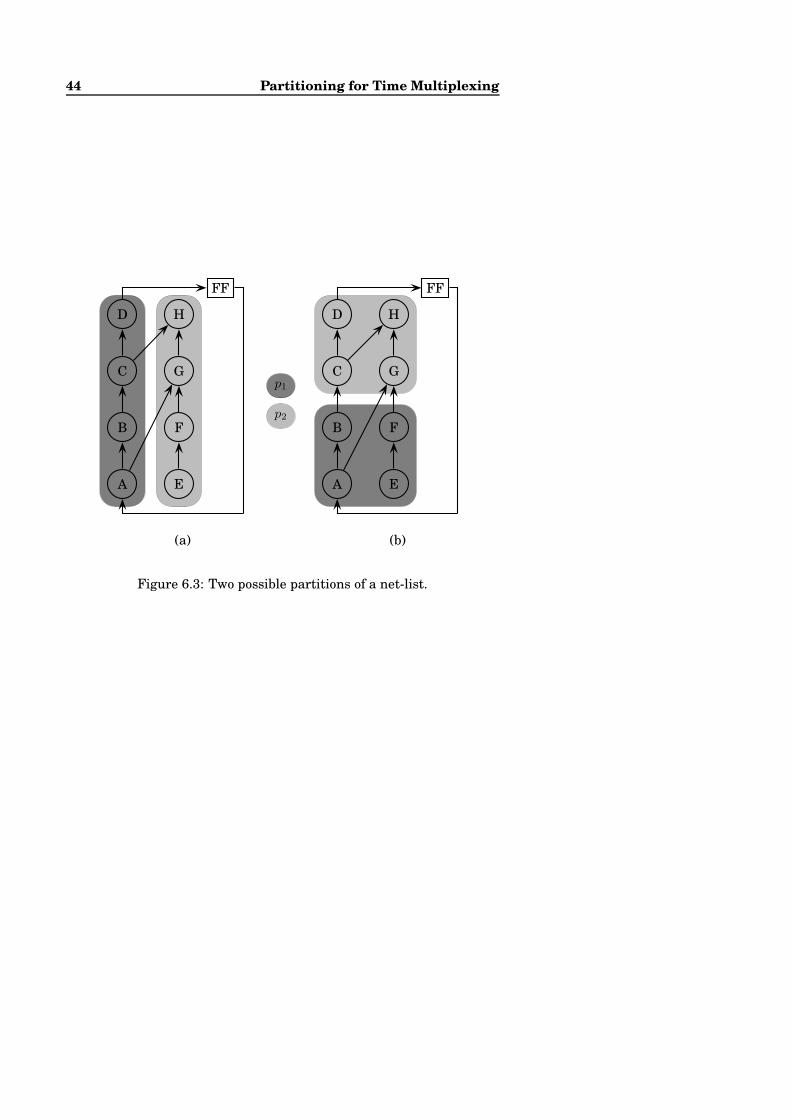
44 Partitioning for Time Multiplexing
p1
p2
(a)
FF
A
B
C
D
E
F
G
H
(b)
FF
A
B
C
D
E
F
G
H
Figure 6.3: Two possible partitions of a net-list.

6.2 The Partitioning Problem 45
(a) A B FF C
(b) A B C
Figure 6.4: Data dependency. (a) the net-list, (b) the dependency graph.
nodes {E, F, G, H} goes to, p2, the second partition. In (b) the parti-
tions are {A, B, E, F} and {C, D, G, H}. Both in (a) and (b) the size of
each partition is 4 nodes, so they use the same amount of resources.
However, the time to execute one iteration, corresponding to one clock
cycle in the net-list, is different. In (a), the data has to propagate
through 4 nodes in each partition. The total time for one iteration is
T = 8Tnode + 2Treconfigure. For the other case, (b), some nodes can be
evaluated in parallel within the partitions. The time for one iteration
is T = 4Tnode + 2Treconfigure.
The critical path in the net-list is the longest path of nodes that can-
not execute in parallel. Partitioning does not increase parallelism, so
executing all partitions in sequence cannot be faster than the propaga-
tion delay of the critical path of the non-partitioned net-list. Thus the
critical path in the non partitioned net-list is a lower bound of the sum
of the critical paths in the partitions. The only time overhead of using
a TMFPGA with a partitioning with minimal timing is the reconfigura-
tion time. This is the case for the partitioning in figure 6.3(b). We have
developed a partitioning algorithm that aims at finding a partitioning
with minimal time overhead.
6.2.1 Data Dependency
As mentioned above, data dependencies must be considered during par-
titioning. To handle this, we do not partition the net-list directly. In-
stead we first create a dependency graph from the net-list and then we
partition this dependency graph. The dependency graph represents the
partial order imposed on the nodes by data dependencies. There exist
two kinds of data dependencies, direct data dependency and forward
data dependency. This is illustrated in figure 6.4. Node B uses the re-
sult of node A to produce its output. This is a direct data dependency.

46 Partitioning for Time Multiplexing
Obviously, node A must be evaluated before node B. This is represented
with a solid arc in figure 6.4(b). Forward data dependency is illustrated
by nodes B and C in figure 6.4. In the net-list, the flip-flop is used to
delay the output of B so it will be the input to node C in the next clock
cycle. In a time-multiplexed FPGA, each clock cycle is divided to micro-
steps. At the end of the micro-step where node B is executed, the value
of the flip-flop will be updated, i.e. the value is written to a register in
the register file where node B is placed. The old value of the flip-flop
is overwritten. The overwritten value is the value node C must use in
this iteration. Therefore node C must have already been executed. This
is illustrated in the dependency graph by a dashed arc.
The dependency graph represents a partial order between nodes and
since the partitions are executed in sequence the dependency graph con-
strains the relative placement of nodes to partitions. If there is an arc
from node A to node B in the dependency graph, node A may not be
placed in a later partition than node B. Placing two nodes in the same
partition is always possible. However, it might influence the perfor-
mance. If there is a direct data dependency between two nodes placed
in the same partition, the duration of that partition will be longer. This
is because the signal has to propagate through two nodes before all
outputs are stable. If the critical path is longer than the number of
partitions, this is unavoidable. Forward data dependencies represent
the read and write order of registers. Those do not introduce delays in
a partition, since reading from and writing to registers are part of the
reconfiguration.
6.2.2 Dependency Loops
As described above, partitioning is similar to scheduling. Indeed, the
partitioning problem can be formulated as a scheduling problem. Par-
titioning a net-list to n partitions is the same as scheduling the com-
binatorial nodes in the corresponding dependency graph such that at
times t0, . . . , tn−1 no nodes are executing. The times t0, . . . , tn−1 are the
reconfiguration times. All nodes executed in the time interval [tk−1, tk]are placed in partition k. The schedules for the partitions in figure 6.3
are shown in figure 6.5. For partition (a) the reconfiguration takes place
at times 0 and 4 and for partition (b) at times 0 and 2. When treating
partitioning as a scheduling problem, timing aspects can be handled by
enforcing a deadline for the schedule.
Scheduling is a well known problem in many areas. For example

6.2 The Partitioning Problem 47
(a)
A B C D E F G H
time 1 2 3 4 5 6 7
(b)
A B C D
E F G H
Figure 6.5: Two possible partitions of a net-list. A thick line indicates
the reconfiguration of the FPGA.
several scheduling algorithms have been developed for high-level syn-
thesis. The conditions for this partitioning problem are, however, dif-
ferent. During high-level synthesis, an acyclic task graph is scheduled.
For the TMFPGA partitioning problem, the dependency graph is not
acyclic. Figure 6.6(a) shows one of several possible net-lists with cyclic
data-dependency. Figure 6.6(b) shows the corresponding dependency
graph. There is a direct data dependency from B to A and a forward
data dependency from A to B, thus giving a cyclic dependency. The
scheduling algorithms from high-level synthesis cannot be applied di-
rectly to this partitioning problem. If the dependency graph could be
transformed such that the resulting graph is acyclic, any scheduling
algorithm could be used.
Assuming that the net-list does not have any combinatorial loops,
the direct data dependencies form an acyclic graph. Therefore any loop
in a data dependency graph must contain at least one forward data
dependency. A forward dependency enforces the order of reading from
and writing to a flip-flop. The old value must be read before the new one
is written. Adding one register to temporary store the new value until

48 Partitioning for Time Multiplexing
(a) FF
B A
(b)
B A
(c) FFC
B A
(d)B A
C
Figure 6.6: Cyclic dependency. (a) the net-list, (b) the dependency
graph, (c) the transformed net-list, (d) the transformed dependency
graph.
the flip-flop can be updated, will remove this dependency. We assume
that in a TMFPGA a register can only be updated from the output of
a LUT, i.e. there is no direct register to register transfer. To move the
value from the temporal register to the flip-flop, it has to pass through
a LUT. This dummy LUT is created by adding one node to the net-list.
This process is depicted in figure 6.6. A dummy node C is added to the
net-list in 6.6(a). The added node is placed between the node updating
the flip-flop, B, and the flip-flop. The resulting net-list is shown in 6.6(c)
and its corresponding dependency graph in 6.6(d). The arc from A to B
in the dependency graph is replaced by one from B to C and one from A
to C. Since there are no paths from A to B after the transformation, the
original loop is broken. There is no outgoing arc from the added node
C, so C cannot be involved in any loop. This ensures that no new loops
are created during the transformation.
Breaking all loops in the dependency graph using the transforma-
tion described above gives an unnecessary overhead. If all nodes in a
loop are placed in the same partition no dependencies are violated and
no additional nodes are needed. Our approach is to ignore some of the
forward data dependencies. This is further explained in section 6.3.1.
Ignoring some arcs in the dependency graph results in an acyclic graph,
called the scheduling graph. This graph is scheduled and if any of the
ignored dependencies is violated, we remove the violated dependency

6.3 The Partitioning Algorithm 49
by the transformation described above. In order to remove the depen-
dency, a node is added to the net-list.
6.3 The Partitioning Algorithm
The main part of our algorithm is the scheduler. The scheduler takes a
net-list, a deadline, and a maximum size for the partitions as input, and
generates a schedule as an output. The scheduling function is explained
in section 6.3.1. Scheduling might fail for two reasons. The generated
schedule might not meet the deadline or, during scheduling, nodes were
added, resulting in a net-list exceeding the partition size. When the
scheduling fails, we relax the size constraint and try to schedule again.
During the new scheduling attempt we use the net-list that was gen-
erated during the previous failed scheduling, i.e. the original net-list
with some additional nodes. We repeat this until a schedule that meets
all constraints is found. The partitioning algorithm is depicted in figure
6.7.
6.3.1 Scheduling
For performance reasons we are using list scheduling to schedule the
net-list nodes. The start time of a node in the derived schedule decides
which partition it is placed in. The scheduling step uses three graph
representations of the design: the net-list, the dependency graph, and
the scheduling graph. The net-list is the LUT equivalent net that is
generated during logic synthesis. The net-list is used to derive timing
information of the nodes. The dependency graph is created from the
net-list, as described in section 6.2.1. From the dependency graph some
arcs are removed to create the scheduling graph. This is an acyclic
graph that is scheduled using list scheduling. The arcs removed during
the creation of the scheduling graph are ignored during scheduling. If
any of the dependencies corresponding to the removed arcs are violated,
the net-list is transformed to remove the dependencies from the design.
The scheduling is depicted in the lower part of figure 6.7.
To create the scheduling graph we first find all nodes that belong
to a loop in the dependency graph. This is the problem of finding all
strongly connected components, which can be done in linear time by
two depth-first traversals of the graph [CLR90].
From the dependency graph, all forward data dependency arcs end-
ing in a node from a loop are removed. After removing these arcs, the

50 Partitioning for Time Multiplexing
PARTITION(net_list){
size = net_list.size/nr_partitions
while(schedule_fails){
net_list = SCHEDULE(net_list, size, deadline)
size=max(size+1, net-list.size/nr_partitions)
}
}
SCHEDULE(net_list, size, deadline){
create_scheduling_graph
for partition = 1 to number_of_partitions{
calculate_ASAP
calculate_ALAP
while(not_full(partition) and all_nodes_are_not_scheduled){
possible = get_all_possible_nodes
node = get_highest_priority(possible)
add(node, partition)
}
check_violations_and_modify_net_list
}
if(unscheduled_nodes_exist OR deadline_missed)
signal failure
return the modified net_list
}
Figure 6.7: The partitioning algorithm.

6.3 The Partitioning Algorithm 51
resulting graph is acyclic. This is the scheduling graph. At this point
only the arcs in the dependency graph are removed, the net-list is un-
changed. The dependencies represented by the removed arcs will be
ignored during scheduling. In figure 6.6(b) the arc from A to B will be
removed and in figure 6.6(d) no arcs will be removed since there are no
loops.
When the scheduling graph has been created, it is scheduled using
list scheduling. List scheduling is an iterative process. In each itera-
tion, one node is selected. The selected node is scheduled, i.e. placed in
a partition. To chose which node to select, a set of possible nodes is cre-
ated. A node is eligible for selection if it is not already scheduled and all
its predecessors in the scheduling graph are scheduled. From the set of
possible nodes, the node with the highest priority is selected. The way
of assigning priorities is described in section 6.3.2. The scheduling loop
is repeated until all nodes are scheduled.
The first n1 selected nodes are placed in partition 1, the following
n2 nodes are placed in partition 2 and so on. How we decide about the
sizes of the partitions is explained in section 6.3.4.
During scheduling, when a partition is filled, the unscheduled nodes
will be scheduled in a later partition than the scheduled nodes. At this
time it is easy to check if there are any dependencies that cannot be ful-
filled. Only the removed forward data dependencies need to be checked.
A dependency cannot be fulfilled if the corresponding arc goes from an
unscheduled node to a scheduled node. After filling one partition, if we
detect that an ignored dependency will be violated, it is removed from
the net-list. This is done by the transformation shown in figure 6.6. All
three graphs are transformed. The added dummy node is treated in the
same way as any other nodes. When all its predecessors in the schedul-
ing graph are scheduled, it will be placed in the set of possible nodes
and it will eventually be selected for scheduling.
6.3.2 The Priority Function
Due to the nature of list scheduling, there is no problem to distribute
the nodes evenly among the partitions. We do not think that the num-
ber of nodes added due to violated data dependencies is a problem ei-
ther. The major concern is to find a schedule that meets the deadline.
The priority function was designed to address this issue.
One way to find a tight schedule is to minimise the critical paths, i.e.
the depths, of the partitions. The priority function does this by giving

52 Partitioning for Time Multiplexing
(a)
ASAP = n ASAP = n + 1
A
B
C
D
partition 1
(b)
ASAP = n + 1 ASAP = n + 2
C
B D
Figure 6.8: A node can have different ASAP values for different parti-
tions. (a) before recalculation of the ASAP values and (b) after recalcu-
lation.
higher priorities to nodes that will not increase the critical path of the
current partition, and a lower priorities to nodes that will increase it.
When nodes are added to a partition, the inverse of the depth of the
nodes in the net-list can be used as a priority. Nodes with depth one
have the highest priority, followed by nodes with depth two and so on.
The depth of a node can be found by doing ASAP scheduling of the net-
list. Observe that it is not the scheduling graph that is used to calculate
the ASAP value. It contains both direct and forward data dependencies,
since a forward data dependency does not correspond to a propagation
delay, but only to the read and write order of the registers.
The procedure described above is used for the first partition. For
later partitions, the use of the original ASAP as priority is not optimal.
In figure 6.8(a) node A and B have ASAP = n. Node A is scheduled
in partition 1 while there is no space for node B. Now if both node B
and C are scheduled in partition 2 both nodes will have a depth of 1
in that partition. Therefore both nodes should have the same priority
for partition 2. To solve this, we recalculate the ASAP value for all
unscheduled nodes when one partition is full. When the ASAP value is
recalculated all nodes must have an ASAP that is larger than the ASAP
of any scheduled nodes. A consequence of this is that a node can have
different priorities for different partitions.
The purpose of the priority function is to order the nodes. The n1

6.3 The Partitioning Algorithm 53
nodes with the highest priority are scheduled in the first partition, the
next ,n2, nodes in partition 2 and so on. When a partition is full it
is likely that some unscheduled nodes have the same ASAP as some
scheduled nodes. In figure 6.8(a) node A is scheduled, but not node B.
The overall schedule is influenced by the selection criterion for nodes to
be scheduled and nodes to be saved for later partitions. Using only the
inverse ASAP as a priority function is not sufficient. For nodes with the
same ASAP we give a higher priority to nodes with smaller mobility.
The mobility of a node is defined as the length of the time interval it
can be scheduled in without violating the deadline. The mobility can
be calculated by doing ALAP and ALAP scheduling of the net-list and
then for each node mobility = ALAP − ASAP .
We do not define a mathematical function for the priority. Instead
we define an ordering of the nodes in a net-list. For two node A, B
A ≺ B iff (A.ASAP < B.ASAP ) ∨
((A.ASAP = B.ASAP ) ∧ (A.ALAP < B.ALAP ))(6.1)
If two nodes have the same ASAP the node with the smallest ALAP
will have the highest priority. Since the ASAP values are the same, this
is the node with the smallest mobility. For nodes with different ASAP
the node with the smallest ASAP has the highest priority.
6.3.3 Deadline Inheritance
If all nodes were scheduled in decreasing priority order, a close to opti-
mal timing is likely to be found. This is not always possible since the
nodes are scheduled in the partial order represented by the scheduling
graph. During scheduling, one node can be blocked by another node
with lower priority. This happens if there is a forward data dependency
from a low priority node to a high priority node, see figure 6.9. Only
considering the net-list in figure 6.9(a) node D has a high mobility, it
can be scheduled between 1 and 3. However there is a forward data
dependency from D to A, so the low priority node D precedes the high
priority node A in the scheduling graph, shown in figure 6.9(b). We ad-
dress this by what we call deadline inheritance. For all nodes, the ALAP
value must be smaller or equal to the ALAP value of all its successors in
the scheduling graph. This property is not automatically fulfilled since
the ALAP values are calculated in the net-list, which does not contain
the forward data dependencies in the scheduling graph. With deadline
inheritance ALAP of node D will change from 3 to 1, and D becomes a

54 Partitioning for Time Multiplexing
(a) (ASAP, ALAP)
A B C
FF
D
(1, 1) (2, 2) (3, 3) (1, 3)
(b) D A B C
(1, 3) (1, 1) (2, 2) (3, 3)
Figure 6.9: A net-list (a) and the corresponding scheduling graph (b).
With deadline inheritance the ALAP of node D will change from 3 to 1.
high priority node. The ALAP value for the nodes is calculated by first
doing ALAP scheduling of the net-list followed by deadline inheritance
during a depth-first traverse of the scheduling graph.
6.3.4 The Size of the Partitions
The list scheduler adds one node at a time to the current partition. The
question is “how many nodes should be placed in each partition”? One
way is to divide the nodes evenly among the partitions. Our experi-
ments showed that this works for some net-lists, but for others it does
not generate a minimal schedule length.
When a node with ASAP equal to n is added to a partition, it means
that all nodes with ALAP smaller or equal to n must also be scheduled
in that partition, or the deadline will be missed. To avoid missing the
deadline, before adding node to a partition we check that all other nodes
with ALAP less or equal to the ASAP of this node will also fit in this
partition. If there is not enough space in the partition for all these
nodes we consider the partition to be full. This check only needs to be
done when the critical path of a partition is extended.
Our criteria for a partition to be full is either that a maximum num-

6.3 The Partitioning Algorithm 55
Table 6.1: MCNC Partitioning93 benchmarks characteristics.
net-list nodes ff depth strongly connected
components
c5315 606 0 14 -
c6288 1199 0 45 -
c7552 643 0 13 -
s9234 373 138 16 1
s13207 1006 450 18 10
s15850 1256 540 22 9
s38417 3361 1464 15 10
s38584 4082 1300 20 41
ber of nodes has been added or adding one more node will lead to a
missed deadline. That is adding one more node will increase the critical
path in the partition and there is not enough space left in the partition
to add all nodes that must be scheduled in the same partition.
6.3.5 Experimental results
We have implemented our algorithm in Java and run it on the MCNC
Partitioning93 benchmark circuits. We used the largest circuits with a
critical path of at least 8 nodes. The experiments were run on a SUN
Ultra-1 SPARC with 192 MB memory. The Java Virtual Machine used
was Solaris VM, Java version 1.2.1. In all our experiments we divided
the net-list to 8 partitions. The benchmark characteristics are shown
in table 6.1.
In our experiments we focused on minimal timing. The deadline for
the schedule was set to the depth of the net-list, i.e. the critical path.
With this timing constraint, the partitioning algorithm was run, both
with and without deadline inheritance. The results are shown in table
6.2.
The column labelled ’nodes added’ shows the number of nodes added
to the net-list by the partitioning algorithm. For the combinatorial
circuits no nodes are added since all direct data dependencies are re-
spected during scheduling.
The size increase of the partitions is shown both in number of nodes
and in percentage. For some circuits the space added to the partitions
is smaller than the number of nodes added to the net-list. This is pos-

56 Partitioning for Time Multiplexing
Table 6.2: Partitioning results.
net-list no deadline inheritance with deadline inheritance
nodes increase of cpu nodes increase of cpu
added partition size (s) added partition size (s)
nr % nr %
c5315 0 0 0 0.26 0 0 0 0.26
c6288 0 0 0 0.36 0 0 0 0.39
c7552 0 0 0 0.38 0 0 0 0.42
s9234 0 0 0 0.19 0 0 0 0.21
s13207 33 4 3.2 0.98 22 3 2.4 1.06
s15850 39 5 3.2 0.99 36 5 3.2 1.01
s38417 14 17 4.0 23.5 11 1 0.2 2.76
s38584 60 7 1.4 3.19 61 7 1.4 3.38
sible because there is some free space even for a minimal size of the
partitions. i.e. free space = netList.size modulo nrPartitions.
The experiments show that deadline inheritance can decrease the
number of nodes added during partitioning. It also improves timing.
This is clear for the circuit s38417. Without deadline inheritance the
partition size is increased by 17 before the deadline is met. This made
space for 8*17=136 nodes, but only 14 were used. With deadline inher-
itance the deadline was met after increasing the size of the partitions
by one.
Our experiments showed that the algorithm can partition net-lists
with up to 4000 nodes in less than 4 seconds. This was done without
any timing overhead and with a space overhead of up to 3.2%.

CHAPTER 7
CONCLUSIONS
7.1 Summary
Improving the productivity in the design of embedded systems is a im-
portant research topic. We have presented several contributions that
can improve the productivity in the development of image processing
systems. As part of the WITAS UAV project we are developing a pro-
totype UAV. The material presented here consists of our experiences
from the the development of the vision sub-system for the WITAS UAV
prototype.
We have developed a computational model, IP-DFG, which is suit-
able for modelling of complex image processing algorithms. IP-DFG is
based on boolean DFGs which have been extended with hierarchy and
better support for token consumptions and iterations.
We have been using IP-DFG as the computational model in a frame-
work for complex image processing modelling and implementation. The
framework is called IPAPI and covers the design process from system
level modelling to optimised implementation. IPAPI is suitable for co-
simulation with other parts of a large system.
Seen as a run time system IPAPI provides three functional aspects,
data processing, memory management and scheduling. Data process-
ing corresponds to the firing functions in an IP-DFG. The firing of the
actors are captured in the scheduler and the memory manager handles
the tokens. To create an IPAPI model of an algorithm, the designer cap-
tures the semantic in a IP-DFG graph, and provides an implementation
of the algorithm specific firing functions, that is, the image operations

58 Conclusions
that are unique for this algorithm.
IPAPI provides more flexibility compared to a traditional task based
run time system. It is possible for IPAPI to dynamically combine differ-
ent algorithms and adapt the size of the image regions they are applied
to. This flexibility does not introduce more complexity during the im-
plementation. Instead the memory manager and scheduler in IPAPI
manages the dependencies introduced by the flexibility.
We have been using IPAPI to optimise a few typical image process-
ing algorithms within the WITAS project for the PowerPC processor.
The optimised implementations take full advantage of the AltiVec unit,
a vector unit in the PowerPC processor. With this optimised imple-
mentation we achieved sufficient computational power in the WITAS
on board system.
We also present an algorithm for temporal partitioning. This algo-
rithm is tailored to be used for time multiplexed FPGAs and makes it
possible to use existing FPGA tools for time multiplexed FPGAs. This
can be used to increase the performance for some actors by using a
FPGA accelerator.

BIBLIOGRAPHY
[AK00] P. Andersson and K. Kuchcinski. Performance Oriented
Partitioning for Time-Multiplexed FPGAs. In the Proceed-
ings of the Euromicro Symposium on Digital System Design,
September 2000.
[AKND02] P. Andersson, K. Kuchcinski, K. Nordberg, and P. Doherty.
Integrating a Computational Model and a Run Time Sys-
tem for Image Processing on a UAV. In the Proceedings
of the Euromicro Symposium on Digital System Design,
September 2002.
[AUV] AUVSI - The Association for Unmanned Vehicle Systems
International. http://www.auvsi.org/.
[Buc93] J. T. Buck. Scheduling Dynamic Dataflow Graphs With
Bounded Memory Using the Token Flow Model. PhD the-
sis, University of Carlifornia at Berkeley, 1993.
[BWR01] G. Buskey, G. Wyeth, and J. Roberts. Autonomous He-
licopter Hover Using an Artificial Neural Network. In
the Proceedings of the IEEE International Conference on
Robotics and Automation (ICRA), volume 2, 2001.
[CLR90] T. H. Cormen, C. E. Leiserson, and R. L. Rivest. Introduc-
tion to Algorithms. MIT Press/McGraw-Hill, 1990.
[DGK+00] P. Doherty, G. Granlund, K. Kuchcinski, E. Sanderwall,
K. Nordberg, E. Skarman, and J. Wiklund. The WITAS Un-

60 BIBLIOGRAPHY
manned Aerial Vehicle Project. In the Proceedings of the
14th European Conference on Artificial Intelligence, 2000.
[EEC+95] T. Edward, I. Eslick, D. Chen, J. Brown, and A. De-
Hon. A First Generation DPGA Implementation. In the
Proceedings of the Third Canadian Workshop on Field-
Programmable Devices, pages 138–143, May 1995.
[EIY+01] J. Evans, G. Inalhan, Yung Soon Jang, R. Teo, and C. J.
Tomlin. Dragonfly: a Versatile UAV Platform for the Ad-
vancement of Aircraft Navigation and Control. In the Pro-
ceedings of the 20th Conference Digital Avionics Systems
(DASC), volume 1, 2001.
[FFM+99] T. Fujii, K. Furuta, M. Motomura, M. Nomura, M. Mizuno,
K. Anjo, K. Wakabayashi, Y. Hirota, Y.-e. Nakazawa, H. Ito,
and M. Yamashina. A Dynamically Reconfigurable Logic
Engine With a Multi-Context/Multi-Mode Unified-Cell Ar-
chitecture. In the Proceedings of the Solid-State Circuits
Conference, pages 364–365, 1999.
[For00] P. E. Forssen. Updating Camera Location and Heading us-
ing a Sparse Displacement Field. Technical Report LiTH-
ISY-R-2318, Dept. EE, Linkoping University, SE-581 83
Linkoping, Sweden, November 2000.
[GGP92] G. R. Gao, R. Govindarajan, and P. Panangaden. Well-
Behaved Dataflow Programs for DSP Computation. In the
Proceedings of the IEEE International Conference on Acous-
tics, Speech, and Signal Processing (ICASSP-92), volume 5,
pages 561–564, 1992.
[Lee91] E. A. Lee. Consistency in Dataflow Graphs. IEEE Trans-
actions on Parallel and Distributed Systems, 2(2):223–235,
April 1991.
[Lee01] E. A. Lee. Overview of the Ptolemy Project. Technical Re-
port Technical Memorandum UCB/ERL M01/11, University
of California, Berkeley, March 2001.
[Lia99] S. Liang. The JavaTMNative Interface: Programmer’s Guide
and Specification. Addison Wesley Longman, Inc., 1999.

BIBLIOGRAPHY 61
[LM87] E. A. Lee and D. G. Messerschmitt. Static Scheduling of
Synchronous Data Flow Programs for Digital Signal Pro-
cessing. IEEE transactions on computers, January 1987.
[LP95] E. A. Lee and T. M. Parks. Data Flow Process Networks.
Proceedings of the IEEE, 83(May):773–801, May 1995.
[NFW+02] K. Nordberg, P. E. Forsen, J. Wiklund, P. Doherty, and P. An-
dersson. A Flexible Runtime System for Image Processing
in a Distributed Computational Environment for an Un-
maned Aereal Vehicle. In the proceedings of the 9th Interna-
tional Workshop on Systems, Signals and Image Processing,
IWSSIP, November 2002.
[PEM] Motorola literature Distribution, P.O. Box 5405, Denver,
Colorado 80217. AltiVec Technology, Programming Envi-
ronments Manual.
[PIM] Motorola literature Distribution, P.O. Box 5405, Denver,
Colorado 80217. AltiVec Technology, Programming Interface
Manual.
[SV98] S. M. Scalera and J. R. Vazquez. The Design and Implemen-
tation of a Context Switching FPGA. In the Proceedings of
the IEEE symposium on FPGAs for Custom Computing Ma-
chines, pages 78–85, 1998.
[TCJW97] S. Trimberger, D. Carberry, A. Johnson, and J. Wong. A
Time-Multiplexed FPGA. In the Proceedings of the Field-
Programmable Custom Computing Machines, pages 22–28,
1997.