MODELLING AND COMPUTATION IN GEOPHYSICAL

EXPLORATION

by

Yile Zhang

A thesis submitted in partial fulfillment of the requirements for the degree of

Doctor of Philosophy

in

Applied Mathematics

Department of Mathematical and Statistical Sciences

University of Alberta

c⃝Yile Zhang, Winter 2016

Abstract

Mathematical model and numerical computation play a pivotal role in modern geo-

physical exploration. By applying computational algorithms to the observed field

data, the underground structure can be inferred. This process is generally referred

as a geophysical inversion problem. However, due to the model complexity, nu-

merical stability and computing time, solving a geophysical inversion problem is

a very challenging task. A typical inversion problem may involve several million

of unknowns, and this frequently requires considerable amount of computing time

even by using a super-workstation.

This thesis focuses on modelling and developing fast and efficient numerical

algorithms for geophysical exploration. By recognizing a Block-Toeplitz Toeplitz-

Block (BTTB) structure in a potential field inversion problem and combining the

conjugate gradient method with the BTTB structure, a class of efficient numerical

schemes are proposed. From the simulation results applied to synthetic and field

data, we conclude that the proposed schemes significantly improve the stability and

accuracy of a downward continuation problem, and they are more superior to the

existing methods. Since a regularization process inherently induces distortion in the

inversion solution, we construct a novel non-regularized inversion scheme based on

a multigrid (MG) technique. The MG based scheme not only preserves the stability

ii

of a regularization method, but it also induces less distortion in the reconstructed

magnetization solution.

We expand our 2D results to a 3D gravity field inversion by proposing a 2D

multi-layer model to approximate the density distribution. Based on the multi-layer

model, an efficient 3D inversion scheme is proposed, in which all formulation in-

cluding the regularization, preconditioning and inversion are conducted under a

BTTB-based framework. Mathematical analysis for convergence and consistency

are presented, and a multi-resolution simulation confirms the efficiency and accu-

racy of the proposed numerical scheme.

As an indispensable tool in high precision exploration, electromagnetic (EM)

method is frequently applied to reconstruct the conductivity distribution. We pro-

pose an implicit ADI-FDTD scheme to model the diffusion behavior of the EM

wave. The time and space grids in our proposed scheme can be much larger than

that used in the conventional Du-Fort-Frankel method, while more accurate nu-

merical solution is obtained. Numerical analysis and computational simulation are

presented to demonstrate the effectiveness of the proposed scheme.

iii

Preface

The research conducted for this thesis forms part of research collaboration with

Prof. Yau Shu Wong and Dr. Jian Deng at the University of Alberta, Sha Lei and

Julien Lambert at TerraNotes Ltd Geophysics, Prof. Dong Liang at York University,

Dr. Wanshan Li at Shandong University, and Yuanfang Lin at East China Normal

University. I was the key investigator of all the research projects in Chapters 2-5.

The main results of Chapter 2 of this thesis have been published as Yile Zhang,

Yau Shu Wong, Yuanfang Lin, An Improved Conjugate Gradient Method for Down-

ward Continuation of Potential Field Data, Journal of Applied Geophysics, 2016,

126, 74 - 86. I was responsible for algorithm design, numerical simulation and

manuscript composition, Prof. Yau Shu Wong was involved in the scheme design,

numerical analyses and manuscript improvement. Yuanfang Lin was involved in

literature study.

The main results of Chapter 3 of this thesis have been published as Yile Zhang,

Yau Shu Wong, Jian Deng, Sha Lei, and Julien Lambert, Numerical Inversion

Schemes for Magnetization Using Aeromagnetic Data, International Journal of Nu-

merical Analysis and Modeling, 2015, 12 (4) 684 - 703. I was responsible for the

scheme design, numerical simulation and analysis, and manuscript writing, Prof.

Yau Shu Wong provides the idea of the scheme and routine of research, and in-

iv

volved in numerical analysis of simulation results, Dr. Jian Deng, Julien Lambert

and Sha Lei were involved in the manuscript improvement, and Sha Lei was re-

sponsible for providing the geophysical data.

The main results of Chapter 4 of this thesis have been published as Yile Zhang,

Yau Shu Wong, BTTB-based Numerical Scheme for 3D Gravity Field Inversion,

Geophysical Journal International, 2015, 203(1), 243 - 256. I was responsible

for the model construction and algorithm design, theoretical analysis, numerical

simulation and manuscript writing. Prof. Yau Shu Wong was involved in algorithm

design, numerical analysis for simulation, and manuscript improvement.

The main results of Chapter 5 of this thesis have been published as Wanshan

Li, Yile Zhang, Yau Shu Wong and Dong Liang, ADI-FDTD Method for Two-

dimensional Transient Electromagnetic Problems, Communications in Computa-

tional Physics, 2016, 19(1), 94 - 123. I am the corresponding author, and proposed

the basic model and corresponding algorithm, I was also responsible for numerical

simulation and manuscript writing. Dr. Wanshan Li was responsible for numerical

simulation, theoretical proof, and manuscript writing. Prof. Yau Shu Wong gave the

idea and the routine of the study, and involved in manuscript improvement. Prof.

Dong Liang was involved in manuscript improvement.

v

Acknowledgement

As time passing to the completion of my Ph.D study, first and foremost, I would like

to express my very great appreciation to my supervisor Prof. Yau Shu Wong. I feel

very lucky and grateful of being accepted as his PhD student. He showed me the

skills of research, the way of professional presenting and discussion, how to solve

mathematical problems from industrial areas and how to form good professional

research habits. He always encourages me to pursue a higher goal in life, and

provides invaluable suggestions in career planning. I am also very grateful for his

careful reading through this long thesis and helping me with the structures, language

and typos. The main part of this thesis comes from four papers we collaborated.

I am very grateful to all committee members of my thesis defense for their

precious time and valuable work. Especially, I would like to thank Prof. Peter

Minev, Prof. Cristina Anton, Prof. Bin Han and Prof. Xinwei Yu, Thanks for your

invaluable time and patience for reading through this long thesis.

Special thanks go to my research group colleague Dr. Jian Deng, who always

stands by me and give me good idea of research.

Finally, I would like to reserve my gratitude to my parent, Without their support,

understanding and love, I would have never completed this thesis and my Ph.D

program.

vi

List of Figures

2.1 Pseudo-magnetic field on the ground level (h=0 m). . . . . . . . . . 28

2.2 The upward continuation of the pseudo-magnetic field in Figure 2.1

to the elevation of (a) h=50 m; (b) h=250 m. . . . . . . . . . . . . . 29

2.3 RMS vs µ graph for (a) TR method; (b) AIT method; (c) BTTB-

RRCG method . . . . . . . . . . . . . . . . . . . . . . . . . . . . 30

2.4 RMS vs µ graph for TR method under the different level of noise. . 30

2.5 The downward continuation with ∆h = 200 m for the 0.005%

noised magnetic field in Figure 2.2(b) by using (a) TR; (b) AIT;

(c) TS and (d) BTTB-RRCG method. . . . . . . . . . . . . . . . . 31

2.6 The downward continuation error distribution by (a) TR; (b) AIT;

(c) TS and (d) BTTB-RRCG method. . . . . . . . . . . . . . . . . 32

2.7 The downward continuation error distribution for 5% noised data

by (a) TR;(b) AIT; (c) BTTB-RRCG method. . . . . . . . . . . . . 35

2.8 Synthetic density model. . . . . . . . . . . . . . . . . . . . . . . . 37

2.9 Generated field by density model in Figure 2.8. . . . . . . . . . . . 37

2.10 The downward continuation results by (a) TR;(b) AIT; (c) BTTB-

RRCG method. . . . . . . . . . . . . . . . . . . . . . . . . . . . . 38

2.11 The downward continuation error distribution for by (a) TR;(b)

AIT; (c) BTTB-RRCG method. . . . . . . . . . . . . . . . . . . . . 38

2.12 (a) The real magnetic field data at h = 0 m;(b) The upward contin-

uation by ∆ = 200 m of the field data in Figure 2.12(a) . . . . . . . 39

2.13 The downward continuation by ∆h = 200 m for 2.5% noised real

field data by (a) TR;(b) AIT; (c) BTTB-RRCG method. . . . . . . . 41

2.14 The downward continuation error distribution for 2.5% noised real

field data by (a) TR;(b) AIT; (c) BTTB-RRCG method. . . . . . . . 41

2.15 The downward continuation by ∆h = 200 m after tailoring for

2.5% noised real field data by (a) TR;(b) AIT; (c) BTTB-RRCG

method. . . . . . . . . . . . . . . . . . . . . . . . . . . . . . . . . 42

2.16 The downward continuation error distribution after tailoring for 2.5%

noised real field data by (a) TR;(b) AIT; (c) BTTB-RRCG method. . 43

2.17 Convergence rate of BTTB-RRCG method in the real field data ap-

plication, where e = ||ATh − T0||2. . . . . . . . . . . . . . . . . . 44

3.1 Forward Model. . . . . . . . . . . . . . . . . . . . . . . . . . . . . 48

3.2 Two-grid and V-cyle MG. . . . . . . . . . . . . . . . . . . . . . . . 52

3.3 Initial magnetization distribution. . . . . . . . . . . . . . . . . . . . 56

3.4 Magnetic field data at different depths. . . . . . . . . . . . . . . . . 57

vii

3.5 Convergence rate of CG, RRCG, PCG and MG method at tolerance=1∗10−3. . . . . . . . . . . . . . . . . . . . . . . . . . . . . . . . . . . 60

3.6 Inversion of the magnetic field at h=250 m by CG, RRCG, PCG and

MG method. . . . . . . . . . . . . . . . . . . . . . . . . . . . . . . 60

3.7 Error vs noise level for the CG, RRCG, PCG and MG method under

tolerance=10−2. . . . . . . . . . . . . . . . . . . . . . . . . . . . . 62

3.8 Original field data and selected window W. . . . . . . . . . . . . . 64

3.9 Test case I. . . . . . . . . . . . . . . . . . . . . . . . . . . . . . . 64

3.10 Inversion results for test case I with tolerance 3 ∗ 10−1 . . . . . . . 65

3.11 Inversion result for test case I at depth h=50 m . . . . . . . . . . . . 67

3.12 Inversion result for test case I at depth h=100m . . . . . . . . . . . 68

3.13 Test case II. . . . . . . . . . . . . . . . . . . . . . . . . . . . . . . 69

3.14 Inversion result for test case II at h = 100m. . . . . . . . . . . . . . 70

3.15 Inversion result for test case II with tolerance = 1 ∗ 10−2. . . . . . . 71

4.1 Uniform splitting of a 3D forward gravity model. . . . . . . . . . . 87

4.2 Non-uniform splitting of a 3D forward gravity model. . . . . . . . . 88

4.3 Synthetic density model I. . . . . . . . . . . . . . . . . . . . . . . 99

4.4 Gravity field generated by synthetic model I, unit of the gravity field

in mGal. . . . . . . . . . . . . . . . . . . . . . . . . . . . . . . . . 99

4.5 Inversion result with different constrains. . . . . . . . . . . . . . . . 100

4.6 Inversion result of gravity field without noise and with 2% Gaussian

noise. . . . . . . . . . . . . . . . . . . . . . . . . . . . . . . . . . 102

4.7 Synthetic density model II. . . . . . . . . . . . . . . . . . . . . . . 102

4.8 Gravity field generated by the synthetic model II. . . . . . . . . . . 102

4.9 Inversion result for gravity field in Figure 4.8 with 2% Gaussian noise.103

4.10 Real gravity field data. . . . . . . . . . . . . . . . . . . . . . . . . 104

4.11 Inversion results at location 1, 2 and 3 in Figure 4.10 at four differ-

ent resolutions. . . . . . . . . . . . . . . . . . . . . . . . . . . . . 105

4.12 The logarithm of the number of unknowns versus the logarithm of

the computing time. . . . . . . . . . . . . . . . . . . . . . . . . . . 105

4.13 Inversion with weighting parameter β = 1.4 . . . . . . . . . . . . . 107

4.14 Misfit versus the iteration steps. . . . . . . . . . . . . . . . . . . . 107

5.1 Geometry for the 2D TEM problem with the double line source. . . 115

5.2 Comparison of analytical and numerical solutions computed by the

ADI-FDTD and DF schemes for the vertical EMF (∂tBz) induced

by a double line source on a half-space. Profiles are at (a)0.007 ms,

(b)0.1 ms, (c)3 ms, (d)15 ms after the source current was switched

off. . . . . . . . . . . . . . . . . . . . . . . . . . . . . . . . . . . . 135

5.3 Relative L∞ and L2 errors for the ADI-FDTD and DF schemes . . 136

viii

5.4 Contours of electric field in a half-space computed by the ADI-

FDTD scheme induced by a switched-off 500m wide double line

source at the earth-air interface. Profiles are at (a)3 ms, (b)10 ms,

(c)15 ms, (d)21 ms after source current was switched off. . . . . . . 136

5.5 Model geometry for half-space with large-contrast conductor. . . . . 139

5.6 Profiles of the vertical EMF (∂tBz) by the ADI-FDTD scheme for

the half-space conductor with a 1000:1 contrast. The negative line

source is on the right. Open marks indicate negative values and

dark marks represent positive ones. . . . . . . . . . . . . . . . . . . 140

5.7 Profiles of the horizontal EMF (∂tBx) by the ADI-FDTD scheme

for the half-space conductor with a 1000:1 contrast. The negative

line source is on the right. Open marks indicate negative values. . . 140

5.8 Contours of electric field(the values are the logarithm of E) com-

puted by the ADI-FDTD scheme(on the left) and the DF scheme(on

the right) for the half-space with the conductor of 1000:1, induced

by a switched-off 500m wide double line source at the earth-air in-

terface. . . . . . . . . . . . . . . . . . . . . . . . . . . . . . . . . 144

5.9 Model geometry for overburden and half-space with small-contrast

conductor. . . . . . . . . . . . . . . . . . . . . . . . . . . . . . . . 146

5.10 Profiles of the vertical EMF (∂tBz) by the ADI-FDTD scheme for

the half-space with small contrast conductor model. The negative

line source is on the right. Open marks indicate negative values and

dark marks represent positive ones. . . . . . . . . . . . . . . . . . . 147

5.11 Profiles of the horizontal EMF (∂tBx) by the ADI-FDTD scheme

for the half-space with small contrast conductor model. The nega-

tive line source is on the right. Open marks indicate negative values. 147

5.12 Contours of electric field(the values are the logarithm of E) com-

puted by the ADI-FDTD scheme(on the left) and the DF scheme(on

the right) for the half-space with small contrast conductor mod-

el, induced by a switched-off 500m wide double line source at the

earth-air interface. . . . . . . . . . . . . . . . . . . . . . . . . . . . 149

ix

List of Tables

2.1 Computational errors using TR, AIT, TS and BTTB-RRCG methods 33

2.2 Error of downward continuation by using TR, AIT and BTTB-

RRCG methods with different level of noise . . . . . . . . . . . . . 34

2.3 Storage and computing time by conventional and BTTB-RRCG

methods . . . . . . . . . . . . . . . . . . . . . . . . . . . . . . . . 35

2.4 Error of downward continuation by using TR, AIT and ITM meth-

ods for synthetic gravity data . . . . . . . . . . . . . . . . . . . . . 37

2.5 Error by TR, AIT and BTTB-RRCG methods for real field data . . . 43

3.1 Condition number of the coefficient matrix corresponding to differ-

ent depths. . . . . . . . . . . . . . . . . . . . . . . . . . . . . . . . 56

3.2 Computing time and number of V-cycles of MG with various grid

levels. . . . . . . . . . . . . . . . . . . . . . . . . . . . . . . . . . 57

3.3 Computing time and iteration numbers of various numerical inver-

sion for synthetic data at h=250m. . . . . . . . . . . . . . . . . . . 59

3.4 Relative error of CG and MG method at different depths and tolerance. 60

3.5 Relative error of CG, RRCG, PG and MG with different noise levels

(%). . . . . . . . . . . . . . . . . . . . . . . . . . . . . . . . . . . 62

3.6 Computing time for test case I with tolerance 3 ∗ 10−1 . . . . . . . 66

3.7 Computing time for test case I using RRCG and MG . . . . . . . . 66

3.8 The computing time for test case II. . . . . . . . . . . . . . . . . . 69

4.1 Computing time for inversion of gravity field real data . . . . . . . 105

5.1 Time steps in second for the ADI-FDTD and DF schemes . . . . . 134

5.2 CPU time in second for the ADI-FDTD and DF schemes . . . . . . 136

5.3 Time steps in second for ADI-FDTD and DF schemes . . . . . . . . 140

x

Contents1. Introduction . . . . . . . . . . . . . . . . . . . . . . . . . . . . . . . . . . . . . . . . . . . . . . 1

1.1 Inverse source and scattering problem . . . . . . . . . . . . . . . . . . . . . . . . . . . . . . 4

1.2 Organization of the Thesis . . . . . . . . . . . . . . . . . . . . . . . . . . . . . . . . . . . . . . . . 6

2. Downward Continuation for Potential Field . . . . . . . . . . . . . . . . . . 9

2.1 Mathematical Background . . . . . . . . . . . . . . . . . . . . . . . . . . . . . . . . . . . . . . . . 13

2.2 BTTB-RRCG iterative scheme . . . . . . . . . . . . . . . . . . . . . . . . . . . . . . . . . . . . 19

2.3 Simulation using synthetic data . . . . . . . . . . . . . . . . . . . . . . . . . . . . . . . . . . . 26

2.4 Applications using real field data . . . . . . . . . . . . . . . . . . . . . . . . . . . . . . . . . . 39

2.5 Conclusion . . . . . . . . . . . . . . . . . . . . . . . . . . . . . . . . . . . . . . . . . . . . . . . . . . . . . . 44

3. Numerical Inversion for Magnetization . . . . . . . . . . . . . . . . . . . . . . 46

3.1 Magnetic Field Forward Model . . . . . . . . . . . . . . . . . . . . . . . . . . . . . . . . . . . . 48

3.2 Numerical Simulations . . . . . . . . . . . . . . . . . . . . . . . . . . . . . . . . . . . . . . . . . . . 55

3.3 Concluding Remarks . . . . . . . . . . . . . . . . . . . . . . . . . . . . . . . . . . . . . . . . . . . . . 72

4. 3D Inversion for Gravity Field Data . . . . . . . . . . . . . . . . . . . . . . . . . 74

4.1 Gravity Field Forward Model . . . . . . . . . . . . . . . . . . . . . . . . . . . . . . . . . . . . . 78

4.2 BTTB-based Gravity Inversion . . . . . . . . . . . . . . . . . . . . . . . . . . . . . . . . . . . . 86

4.3 BTTB-based regularization . . . . . . . . . . . . . . . . . . . . . . . . . . . . . . . . . . . . . . . 92

4.4 Numerical Results . . . . . . . . . . . . . . . . . . . . . . . . . . . . . . . . . . . . . . . . . . . . . . . 98

4.5 Concluding Remarks . . . . . . . . . . . . . . . . . . . . . . . . . . . . . . . . . . . . . . . . . . . . . 106

5. ADI-FDTD for 2-D Transient Electromagnetic Problems . . . . .110

5.1 TEM Model . . . . . . . . . . . . . . . . . . . . . . . . . . . . . . . . . . . . . . . . . . . . . . . . . . . . . 114

5.2 Numerical Formulation for ADI-FDTD with Integral Boundary . . . . . . . 116

5.3 Stability analysis of ADI-FDTD in L2 norm . . . . . . . . . . . . . . . . . . . . . . . . 124

5.4 Convergence analysis of ADI-FDTD . . . . . . . . . . . . . . . . . . . . . . . . . . . . . . . 130

5.5 Numerical Simulations . . . . . . . . . . . . . . . . . . . . . . . . . . . . . . . . . . . . . . . . . . . 133

5.6 Concluding Remarks . . . . . . . . . . . . . . . . . . . . . . . . . . . . . . . . . . . . . . . . . . . . . 150

6. Conclusion . . . . . . . . . . . . . . . . . . . . . . . . . . . . . . . . . . . . . . . . . . . . . . .152

Bibliography . . . . . . . . . . . . . . . . . . . . . . . . . . . . . . . . . . . . . . . . . . . . . . .155

viixi

Chapter 1

Introduction

Inverse problems form the basis of modern geophysical exploration. In a practical

survey, most of the observed fields are produced by natural sources, but artificial

sources are frequently used to generate induced fields in some cases [123]. Consider

that the underground geology and the external observed geophysical field are linked

together by a physical law, it is feasible to infer the underground structure from the

observed field.

Predicting the external observable field from given geophysical parameters is

called a forward problem. Inversely, inferring the underground geological structure

from the observed field is an inverse problem, and the reconstructed solution is an

inverse problem solution.

Inverse problem is generally challenging in terms of computation and interpre-

tation [71, 14]. From a numerical prospective, the data obtained from measurement

is always polluted due to the fluctuation of the measuring apparatus, therefore an

inversion scheme should be robust enough for large perturbation. From a mod-

elling prospective, it is impossible to construct an accurate model for the under-

ground structure since the natural geology can be extremely complex. Assumption

1

is usually required to keep the mathematical formulation simple. However, such

simplification also makes the interpretation more difficult.

An effective way to enhance the inversion solution is to increase the inversion

resolution. As a popular method in geophysical exploration, a seismic method pos-

sess more flexibility to achieve a high resolution than other methods [69, 39, 81].

By changing the location of a seismic wave field source, plentiful field data can be

collected to reduce the uncertain of the underground geology. However, even for a

seismic wave method, the accuracy and existence of an inversion solution can not

be guaranteed without using a regularization [5].

The regularization is a critical topic in geophysical inversion. The definition

of a well-posed problem is given by [48, 123], in which a well-posed mathemati-

cal model for a physical problem requires: 1. A solution exists; 2. The solution

is unique and 3. The solution changes continuously with the initial conditions.

Problems that are not well-posed are ill-posed. We define a general geophysical

inversion problem as follows:

A(x) = d, x ∈M, d ∈ D, (1.0.1)

whereD is the domain of observed data, M is the domain of geological model, A is

the forward operator generating the data d from a given model x. Consider the case

of a potential field problem, where the forward operator A is a linear operator. The

observed data is always polluted and resulting a noisy data dε. Denote the inversion

2

solution bym, since the matrixA in (1.0.1) is usually full, huge and ill-conditioned,

the numerical inversion solution m is sensitive to a small change of dε. For a non-

linear inversion problem including an electromagnetic problem and a seismic wave

problem, the non-linearity makes the noise effect even more complicated. It is not

hard to conclude that all geophysical inversion problems are ill-posed.

However, an inversion problem which is ill-posed does not imply that the in-

version solution of an ill-posed problem is useless. In 1977, Tikhonov proposed a

clever way to solve an ill-posed problem [105], in which the problem is approximat-

ed by a family of well-posed problems by introducing additional prior information

and constraints. Thereafter, the basic idea of a regularization has been developed

and extensively applied to all geophysical inversion problems [123]. The regular-

ization is capable of improving the robustness of a numerical scheme regardless of

the problem dimension, and it has been reported that regularization is effective for

1D [55], 2D [96] and 3D [119] geophysical inversion problems. Many progress

have been made in applying the Tikhonov regularization for geophysical inversion

problems. However, in recent years, the geophysical database grows explosively

due to the use of aero-survey and sensor techniques. Processing enormous field da-

ta is now routinely needed to handle survey from satellite data and high resolution

data.

The trend of growing large field data exerts additional challenges to a numerical

inversion scheme. Therefore, developing efficient computing methods for geophys-

3

ical inversion problem is of significance in theoretical study and practical applica-

tions. The main goal of this thesis is to make contributions in the following issues:

(i) How to construct a fast inversion for large scale data without sacrificing the

quality of the solution by using a modest computing resource.

(ii) How to achieve a fast computation for regularization without simplification.

(iii) How to preform a high-resolution inversion.

(iv) How to carry out numerical analysis for inversion schemes under the geo-

physical background.

In the following section, we review the formulation of geophysical problems.

1.1 Inverse source and scattering problem

Geophysical methods are based on studying the observed field generated by dif-

ferent geophysical parameter distributions. The most important geophysical fields

are gravity field, magnetic field, electromagnetic field and seismic wave. Although

these fields are generated by totally different physical parameters, the inversion

process can be classified into two categories.

For the first type, once the underground parameters are fixed, the resulting fields

are determined. A typical example is the gravity inversion, where the observed

gravity fields are uniquely determined by the underground density distribution. The

4

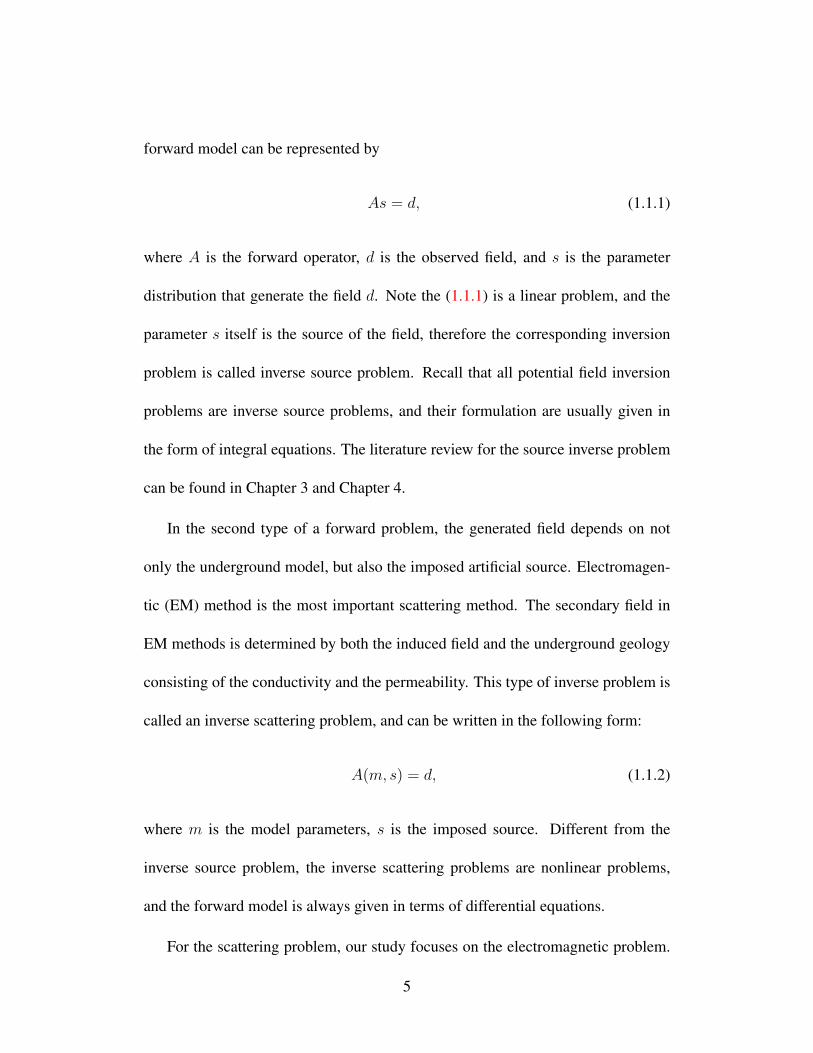
forward model can be represented by

As = d, (1.1.1)

where A is the forward operator, d is the observed field, and s is the parameter

distribution that generate the field d. Note the (1.1.1) is a linear problem, and the

parameter s itself is the source of the field, therefore the corresponding inversion

problem is called inverse source problem. Recall that all potential field inversion

problems are inverse source problems, and their formulation are usually given in

the form of integral equations. The literature review for the source inverse problem

can be found in Chapter 3 and Chapter 4.

In the second type of a forward problem, the generated field depends on not

only the underground model, but also the imposed artificial source. Electromagen-

tic (EM) method is the most important scattering method. The secondary field in

EM methods is determined by both the induced field and the underground geology

consisting of the conductivity and the permeability. This type of inverse problem is

called an inverse scattering problem, and can be written in the following form:

A(m, s) = d, (1.1.2)

where m is the model parameters, s is the imposed source. Different from the

inverse source problem, the inverse scattering problems are nonlinear problems,

and the forward model is always given in terms of differential equations.

For the scattering problem, our study focuses on the electromagnetic problem.

5

The forward formulation of an electromagnetic problem is based on solving the

Maxwell equation, and there are mainly two approaches:

(i) Apply numerical method such as finite difference (FD), finite element (FE)

and integral equation (IE) to solve the problem in time domain and to compute

the transient solution directly.

(ii) Compute the solution in a frequency domain by FD, FE or IE, and then trans-

form the frequency domain solution into the time domain.

A literature review for the EM problems can be found in Chapter 5.

1.2 Organization of the Thesis

The thesis is arranged into five chapters. The first chapter presents a brief intro-

duction of the geophysical inversion problem, and the corresponding time-domain

and frequency-domain formulation are reviewed. In the second chapter, a novel

computation scheme for a downward continuation is investigated. In a time do-

main formulation of a downward continuation, the conjugate gradient (CG) method

is implemented by utilizing the Block-Toeplitz Toeplitz-Block (BTTB) structure.

Unlike a wavenumber domain regularization method, the BTTB-based CG method

induces little artifacts near the boundary. The application of a re-weighted regular-

ization in a space domain significantly improves the stability of the CG scheme for

noisy data. The synthetic data with different level of noise and real field data are

6

used to validate the effectiveness of the proposed scheme. The continuation results

are compared with recently proposed wavenumber domain methods and the Taylor

series method.

In the third chapter, we study the magnetic field inversion problem. We show

that a 3D magnetic field formulation can be converted into a 2D form. By con-

structing a multi-grid scheme, the system matrix preserve the BTTB structure at

each grid level. Consequently, the storage and computational complexity can be

greatly reduced. Comparing with a regularization method, the multigrid method in-

duces much smaller distortion in an inversion process, and preserve the stability of

a regularized method. These properties of the proposed BTTB-MG scheme make it

a good alternative to a regularized method when a high accuracy is required for the

inversion with perturbed data.

In the forth chapter, a 3D gravity field inversion problem is investigated. First, a

novel model for a 3D gravity field formulation is presented, such that the complex

3D density model can be approximated by a sequence of 2D multi-layer models.

The proof of the consistency and convergence for the proposed model are given.

Differed from a conventional 3D inversion method, the proposed method directly

generates a BTTB structure in each 2D layer, such that the 3D inversion scheme is

as efficient as a 2D problem. Both regularization and optimal preconditioning op-

erator can be constructed in terms of BTTB structure. Consequently, very efficient

solvers can be developed, such that tremendous reduction in storage requirement

7

and computing time can be achieved. We applied the proposed scheme for real field

data to reconstruct 3D underground density distribution under different resolutions.

The fifth chapter focuses on developing efficient numerical computation for

eletromagnetic forward model. An alternating direction finite-difference time-domain

(ADI-FDTD) scheme is proposed for a 2D transverse electric (TE) mode electro-

magnetic (EM) propagation problem. Unlike the conventional upward continuation

approach for the earth-air interface, an integral formulation for the interface bound-

ary is developed and it can effectively incorporate to the ADI solver. Stability and

convergence analysis together with an error estimate are presented. Numerical sim-

ulations are carried out to validate the proposed method, and the advantage of the

present method over the popular Du-Fort-Frankel scheme is clearly demonstrated.

The simulations of the electromagnetic field propagation in the ground with anoma-

ly further verify the effectiveness of the proposed scheme.

Finally, it should be mentioned that four scientific papers have been written

based on the work reported in this thesis. The four papers have been published in

International Journal of Numerical Analysis and Modeling, Geophysical Journal

International, Communications in Computational Physics and Journal of Applied

Geophysics.

8

Chapter 2

Downward Continuation for Potential

Field

Downward continuation is frequently applied to enhance the potential field data. It

provides geological information at low elevation by using the field data from high

elevation. In recent years, the aero-gravity and magnetic survey have been wide-

ly used in prospecting [120]. Hence, it is desirable to develop efficient and robust

downward continuation methods to deal with large amounts of aero-potential field

data. According to the physical law, the potential field data at higher elevation con-

tains dim geophysical information, which makes the data less valuable. The poten-

tial field data can be enhanced by using a downward continuation technique, such

that the potential field at lower elevation or even underground within the harmonic

source-free region [78] can be effectively estimated.

In a wavenumber domain (Fourier spectral domain), the continuation can be

carried out by multiplying a continuation factor with the spectrum of the observa-

tion data. Unfortunately, the downward continuation factor grows rapidly as the

continuation distance increases. The high frequency components including noise in

9

the observation data will be amplified and thus resulting a severe polluted solution.

Therefore, using downward continuation in a wavenumber domain is an inherently

unstable process. Using appropriate filters or constrains, stable downward con-

tinuation can be constructed. Dean [32] proposed a method to constrain the high

frequency components. The use of a Wiener filter is investigated in [20, 79]. Re-

cently, Pavsteka et al. [78] propose a robust wavenumber domain method where the

filter is designed based on the characteristics of Tikhonov regularization, Zeng et al.

[117] use an adaptive iterative Tikhonov method to apply Tikhonov filter in each it-

eration in a wavenumber domain. The advantage of a wavenumber domain method

is that the downward continuation process can be accelerated by fast Fourier trans-

form (FFT). It has been proved that an appropriate designed filter can guarantee the

accuracy and stability of downward continuation even for noisy data [78, 117].

Another type of downward continuation method is based on the Taylor expan-

sion, where the potential field at one elevation can be expanded by the potential

field and its vertical derivative terms at another elevation. The success of the Tay-

lor series method depends on the accuracy and stability in computing the vertical

derivative terms. Fedi and Florio [36, 35] propose ISVD method, where the odd

vertical derivatives can be computed in a stable way, and the even order vertical

derivative can be efficiently computed by finite difference. Zhang et al. [118] pro-

pose a truncated Taylor series iterative scheme to achieve robust and stable down-

ward continuation. Ma et al [67] compute the downward continuation by adding an

10

upward continuation and a second vertical derivative at the observation plane, and

the scheme can also be converted to an iterative version. The Taylor series method

is capable of providing very accurate solution when the data are relatively clean,

and the iterative Taylor series method usually has a fast convergence rate.

It should be noted that both the wavenumber domain methods and the Taylor

series methods can be accelerated by FFT. However, the FFT itself can induce an

artifact, and the FFT-induced artifact can be seen in many existing methods, this

is particularly obvious in some iterative wavenumber domain methods [117]. The

FFT-induced error in the downward continuation process has already been studied

by researchers in [107, 24, 78]. To resolve the difficulty, either extrapolation is

needed to extend the original data [78], or a smaller window should be used to

exclude the results near the boundary. For the Taylor series methods, besides the

FFT-induced error, another problem is the robustness for the noisy data. Although

the ISVD method [36, 35] can be applied to compute the odd derivatives in a stable

way, but the even derivatives are still computed by the standard finite difference

which is sensitive to the noise. Other iterative methods such as that based on the

Taylor series has a similar problem [118, 67]. Without a denoising procedure, it is

hard to apply the Taylor series methods for the field data with more than 1%noise.

In summary, the FFT produces an efficient computation with the numerical

complexity of order n log n, where n is the number of unknowns. To apply the

FFT, a continuation process including the regularization is usually converted into

11

the wavenumber domain. For this reason, regularized downward continuation in

a space domain has seldom been investigated. Zhang and Wong [119] propose a

numerical scheme for 3D gravity field inversion, where a special algebraic struc-

ture called Block-Toeplize Toeplize-Block (BTTB) matrix is utilized to make the

scheme efficient.

In this chapter, we consider conjugate gradient (CG) method utilizing the BT-

TB structure for downward continuation problem. The BTTB structure is derived

from the downward continuation formulation in space domain, and it has the same

numerical efficiency as the FFT-based methods. However, compared with the FFT-

based methods, the proposed method induces very small artifact near the bound-

ary, such that neither extrapolation nor tailoring process are required to reduce the

boundary error. This characteristic of the BTTB structure allows the use of an it-

erative scheme without accumulating the error near the boundary. Combining the

BTTB structure with re-weighted regularized conjugate gradient method (BTTB-

RRCG), a stable downward continuation method can be constructed. Here, all for-

mulations are in time domain, such that various space domain regularization stabi-

lizers can be applied. We compare the proposed computational scheme with other

recently proposed schemes for downward continuation. The simulation results for

synthetic and field data demonstrate that the proposed scheme is more accurate and

robust for applications using clean and noisy data.

In section 2.1, the formulation of downward continuation is presented. We

12

briefly introduce the Tikhonov regularized method (TR) [78], adaptive iterative

Tikhonov method (AIT) [117], and stable iterative Taylor series method (ITS) [67].

Section 2.2 focuses on the proposed BTTB-RRCG scheme. In Section 2.3, syn-

thetic field data are used to validate the proposed numerical scheme, and the result

is compared with those obtained by TR, AIT and ITS methods. A Gaussian noise

from 0.1% to 5% of the maximum magnitude of the synthetic data are added to test

the robustness. The error are analyzed by using RMS and the relative error in terms

of L-2 norm and L-∞ norm. Particularly, the FFT-induced error near the boundary

is investigated. In section 2.4, we apply the proposed scheme to the field data, and

similar to the synthetic case, the result is compared with other existing methods.

2.1 Mathematical Background

The relationship between the potential field data at two observation planes is given

by [117]:

T(x, y, h0) =h0 − h

2π

∫ ∞

−∞

∫ ∞

−∞

T(x′, y′, h)dx′dy′

[(x− x′)2 + (y − y′)2 + (h− h0)2]3/2, (2.1.1)

where x and y are the horizontal coordinates, T(x, y, h0) is the observation field at

higher elevation h0, and T(x, y, h) is the unknown field at lower elevation h such

that h0 > h. The downward continuation process is to seek T(x, y, h) at lower

elevation from the potential field T(x, y, h0) at higher elevation.

Denote the kernel as K, the integral equation (2.1.1) can be converted into the

13

following convolution form

T(x, y, h0) =

∫ ∞

−∞

∫ ∞

−∞K(x− x′, y − y′, h0 − h)T(x′, y′, h)dx′dy′, (2.1.2)

which can be further simplified as

T(h0) = K ∗ T(h), (2.1.3)

where ∗ denotes the convolution. According to the convolution theorem,

F(T(h0)) = F(K ∗ T(h)) = F(K) · F(T(h)), (2.1.4)

therefore,

T(h0) = F−1(F(K) · F(T(h))). (2.1.5)

Since

F(K) =

∫ ∞

−∞

∫ ∞

−∞K(x, y)e−2πi(ux+vy)dxdy = e−(h0−h)

√u2+v2 , (2.1.6)

denote T(h0) and T(h) by Th0and Th, respectively, then equation (2.1.3) can be

rewritten into the following matrix form

Th0= F−1ΛFTh, (2.1.7)

where F and F−1 are the Fourier matrices corresponding to a 2D Fourier transform,

and Λ is the continuation kernel K in the wavenumber domain given by (2.1.6).

Consider for h0−h > 0, the kernel e−(h0−h)√u2+v2 is stable, since the high frequen-

14

cy component can be compressed. This explains why an upward continuation is a

stable process.

According to (2.1.7), the most straightforward way to conduct the downward

continuation is

Th = F−1Λ−1FTh0, (2.1.8)

where Λ−1 is given by e(h0−h)√u2+v2 . Obviously, since h0 − h > 0, the kernel

given by e(h0−h)√u2+v2 will amplify all frequency components in Th0

, such that the

solution of Th will be polluted by the high frequency component or noise in Th0.

Denote Th by T, (2.1.8) can be rewritten into a simplified form as

T = Λ−1Th0, (2.1.9)

where T and Th0are the potential field in wavenumber domain with heights h and

h0.

According to the analysis above, the downward continuation is an inherently

unstable process, and conventionally, there are mainly two approaches to resolve

this issue: Tikhonov regularization in wavenumber domain and the Taylor series

method.

15

2.1.1 Wavenumber domain Tikhonov regularization method

Let us denote the downward continuation formulation (2.1.1) into the following

form:

Th0= AT, (2.1.10)

where A is the upward continuation operator. As we have discussed early, solving

(2.1.10) is an ill-posed problem, which is equivalent to compute (2.1.9). Tikhonov

and Arsenin [105] proposed an effective way to solve this kind of problem. In-

stead of solving (2.1.10) directly, they converted the problem into the following

minimization problem:

min||Wd(AT − Th0)||2 + µ||Wm(T − Tref)||2, (2.1.11)

where µ is the regularization parameter, Wd and Wm are the data weighting matrix

and model weighting matrix, respectively, Tref is the prior information, and || · · · ||

denotes the L2-norm. In a downward continuation, Tref is usually a zero vector. Let

Wd and Wm be the identity matrix, then the solution of (2.1.11) can be given by

TTik = (ATA + µI)−1ATTh0. (2.1.12)

Convert (2.1.12) into a wavenumber domain, we have [117]:

TTik =Λ2

Λ2 + µΛ−1Th0

= LTikΛ−1Th0

. (2.1.13)

16

Compare (2.1.13) with (2.1.9), it can be seen that LTik is the Tikhonov regular-

ization filter in a wavenumber domain, which is given by

LTik =e−2∆h

√u2+v2

e−2∆h√u2+v2 + µ

. (2.1.14)

where ∆h = h0 − h is the downward continuation distance.

Based on (2.1.14), Zeng et al. [117] proposed an iterative Tikhonov scheme in

the following form:

Tn = Tn−1 +e−2∆h

√u2+v2

e−2∆h√u2+v2 + µ

Λ−1Rn−1, (2.1.15)

with the initial value T0 is given by T0 = LTikΛ−1Th0

, Rn = Th0− Λ−1Tn.

Actually, the Tikhonov regularization (2.1.11) may have different forms with

different Tikhonov regularization stabilizers. Applying the Tikhonov formulation

given in [106], Pasteka et al. [78] proposed another efficient Tikhonov regulariza-

tion filter in a wavenumber domain in the form of

LTik =1

1 + µ(u2 + v2)e∆h√u2+v2

. (2.1.16)

Our numerical simulations show that as a one-step Tikhonov regularization fil-

ter, (2.1.16) is better than (2.1.14) in the robustness and accuracy, while the iterative

version of (2.1.14) is slightly better than (2.1.16).

17

2.1.2 Taylor series methods

Differed from the FFT-based iterative method, the Taylor series method is to express

the potential field at the elevation h by the potential field at another elevation h0 as

T(x, y, h) = T(x, y, h0) +∂T(x, y, h0)

∂z∆h+

1

2!

∂2T(x, y, h0)

∂z2∆h2 + · · ·

+1

m!

∂mT(x, y, h0)

∂zm∆hm, (2.1.17)

where ∆h = h0 − h.

The ISVD method proposed by Fedi and Florio [36, 35] uses vertical integrating

the field in a wavenumber domain to compute the odd vertical derivative, which has

a good stability for noisy data. Ma et al. [67] introduced a method to remove the

odd derivative from the Taylor formulation in the following form

T(x, y, h) ≈ 2T(x, y, h0)− T(x, y, h0 +∆h) +∂2T(x, y, h0)

∂z2h20, (2.1.18)

where T(x, y, h0+∆h) is the upward continuation of the observation field T (x, y, h0)

with a continuation distance ∆h. Recall that an upward continuation is a stable

process, therefore the downward continuation scheme (2.1.18) based on upward

continuation should be stable.

Both the ISVD method and Taylor formulation (2.1.18) requires computing the

second vertical derivative by a finite difference. From the Laplace equation, the

second vertical derivative can be computed by a second order horizontal derivative

in x and y direction. Although finite differencing is an efficient way to compute the

18

horizontal derivative [36], it is sensitive to noisy data. In our simulation, assume the

grid size is given by h and to reduce the error to minimum, we apply a second order

central scheme (2.1.19) to compute the second horizontal derivative in the interior,

and the second order forward scheme (2.1.20) to compute the second horizontal

derivative on the boundary, such that the overall numerical derivative is of second

order accuracy.

f ′′(x) =f(x+ h)− 2f(x) + f(x− h)

h2(2.1.19)

f ′′(x) =f(x+ 2h)− 2f(x+ h) + f(x)

h2(2.1.20)

2.2 BTTB-RRCG iterative scheme

We now present a new approach for a downward continuation. Instead of converting

the downward continuation formulation into a wavenumber domain as in (2.1.6), we

work with a space domain formulation and discretize (2.1.1) as

T (x(i), y(i), h0) =N∑

j=1

M∑

k=1

G(x(i), y(i), x′(j), y′(k), h0 − h)T (x′(j), y′(k), h)∆x∆y,

i = 1, 2, · · · , N ∗M, (2.2.1)

where h0 and h are defined as before, N and M are the number of data grids in

the x and y direction, ∆x and ∆y are the grid interval in the x and y direction.

Denote the data points on the lower plane indicated by T (x′(i), y′(j), h), where

i = 1, · · · , N, j = 1, · · · ,M . Renumbering the data grids to T (x′(l), y′(l), h),

19

where l = 1, · · · , N ∗ M , which means that we rearrange the index of the data

without changing the total number of data points.

Thus, (2.2.1) can be rewritten as

T (x(i), y(i), h0) =N×M∑

l=1

G(x(i), y(i), x′(l), y′(l), h0 − h)T (x′(l), y′(l), h)∆x∆y,

i = 1, 2, · · · , N ∗M, (2.2.2)

where

G(i, l, h) =h0 − h

[(x(i)− x(l))2 + (y(i)− y(l))2 + (h− h0)2]3

2

. (2.2.3)

By (2.2.2) and (2.2.3), the original downward continuation formualtion (2.1.1)

can be approximated by the linear system

T0 = GT. (2.2.4)

Here, T0 is the discretized observation field, T is the unknown field data, and G

is a (N ×M) by (N ×M) BTTB matrix generated from the discretization (2.2.2).

The BTTB matrix is given in the following form:

GMN =

G(0) G(−1) · · · G(2−M) G(1−M)

G(1) G(0) G(−1) · · · G(2−M)

... G(1) G(0). . .

...

G(M−2) · · · . . .. . . G(−1)

G(M−1) G(M−2) · · · G(1) G(0)

, (2.2.5)

20

in which each block G(m) is a Toeplitz matrix given by

G(m) =

g(m)0 g

(m)−1 · · · g

(m)2−N g

(m)1−N

g(m)1 g

(m)0 g

(m)−1 · · · g

(m)2−N

... g(m)1 g

(m)0

. . ....

g(m)N−2 · · · . . .

. . . g(m)−1

g(m)N−1 g

(m)N−2 · · · g

(m)1 g

(m)0

, m = 0, 1, · · · ,M − 1, (2.2.6)

where gi is constant along its diagonals and the value is defined by (2.2.3).

One important property of a BTTB matrix is that the first row and the first

column contain all information of a given matrix. Consequently, for the matrix G

given by (2.2.5), we only need to store the first row and first column, such that

the storage requirement for the sensitivity matrix can be dramatically reduced from

(N ∗ M)2 to 2(N ∗ M). It should be noted that for the downward continuation

problem, the BTTB matrix is always a symmetric matrix regardless of the choice

for ∆x and ∆y. Hence, the storage requirement for the sensitivity matrix is further

reduced to N ∗M .

Another important feature of BTTB structure is that any BTTB matrix can be

embedded into a Block-Circulat Circulant-Block (BCCB) matrix as [15]:

CMN =

GMN ×

× GMN

, (2.2.7)

21

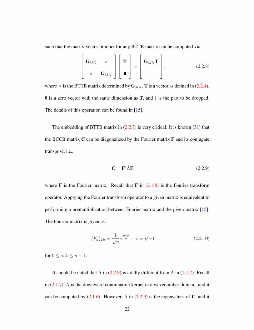
such that the matrix-vector product for any BTTB matrix can be computed via

GMN ×

× GMN

T

0

=

GMNT

†

, (2.2.8)

where × is the BTTB matrix determined by GMN , T is a vector as defined in (2.2.4),

0 is a zero vector with the same dimension as T, and † is the part to be dropped.

The details of this operation can be found in [15].

The embedding of BTTB matrix in (2.2.7) is very critical. It is known [31] that

the BCCB matrix C can be diagonalized by the Fourier matrix F and its conjugate

transpose, i.e.,

C = F∗ΛF, (2.2.9)

where F is the Fourier matrix. Recall that F in (2.1.8) is the Fourier transform

operator. Applying the Fourier transform operator to a given matrix is equivalent to

performing a premultiplication between Fourier matrix and the given matrix [15].

The Fourier matrix is given as:

(Fn)j,k =1√ne

2πijk

n , i =√−1 (2.2.10)

for 0 ≤ j, k ≤ n− 1.

It should be noted that Λ in (2.2.9) is totally different from Λ in (2.1.7). Recall

in (2.1.7), Λ is the downward continuation kernel in a wavenumber domain, and it

can be computed by (2.1.6). However, Λ in (2.2.9) is the eigenvalues of C, and it

22

has different dimension from Λ.

The computation of Λ in (2.2.9) is different from computing Λ in (2.1.6). For

an n by n circulant matrix C, the Λ can be computed via FFT by observing the first

column of Fn is 1√n

1n, where 1n = (1, 1, . . . , 1)T ∈ Rn is the vector consisting of

all ones. Let e1 = (1, 0, . . . , 0)T ∈ Rn, then by using (2.2.9), we have

FnCne1 =1√nΛn1n, (2.2.11)

which implies that Λ can be computed by applying fast Fourier transform to C.

The BTTB matrix has many other attractive properties including the construc-

tion for an efficient preconditioner, and recent work on preconditioners has been

reported in [15].

Now the downward continuation problem (2.1.1) is converted into solving the

linear system (2.2.4). Similar to a wavenumber domain method, the Tihonov regu-

larization (2.1.12) can also be applied. In this study, we consider using the conjugate

gradient type method to solve the regularization problem (2.1.12), since theoretical-

ly it has a rapid rate of convergence [3]. Compared with the steepest decent method

[114, 117], which can be regarded as first order gradient method, the conjugate gra-

dient method is a second order gradient method. Combining the BTTB property

(2.2.9) and (2.2.8) with the RRCG scheme in [123], we develop a BTTB-RRCG

scheme. The details of the standard RRCG scheme can be found in [123]:

RRCG. For the minimization problem given in (2.1.11), denote the observation

23

field Th0by d, and the potential field at the target plane Th by m. Let m0 be an

initial approximation, α0 be the initial regularization parameter. The re-weighted

regularized conjugate gradient (RRCG) algorithm is given as follows.

r0 = Am0 − d, s0 = Wm(m0 − mref),

Iα0

0 = Iα0(m0) = ATW2dr0 + α0Wms0,

for n = 1, 2, 3 · · ·

rn = Amn − d, sn = Wm(mn − mref),

Iαn

n = Iαn(mn)=ATW2drn + αnWmsn,

βαnn = ||Iαn

n ||2/||Iαn−1

n−1 ||2,

Iαn

n = Iαn

n Iαn−1

n−1 , Iα0

0 = Iα0

0 ,

kαnn = (I

αnT

n Iαn

n )/[IαnT

n (ATW2dA + αW2

m)Iαn

n

],

mn+1 = mn − kαnn I

αn

n , γ = ||sn+1||2/||sn||2,

αn+1 =

αn if γ ≤ 1

αn/γ if γ > 1

By combining the discretization process and the properties of BTTB matrix with

the RRCG algorithm, the BTTB-RRCG algorithm is given as follows:

BTTB-RRCG. For the downward continuation problem (2.1.10), denote the obser-

vation field Th0by d, and the potential field at the target plane Th by m.

Step 1. Discretize the upward continuation operator (2.1.1) by using (2.2.2).

Step 2. Generate the matrix G in (2.2.4) in the form of (2.2.5), and a compact

storage format is used to store G.

24

Step 3. Choose an appropriate regularization in time domain, and convert the

problem (2.2.4) into a minimization problem (2.1.11). The regularization stabilizer

is also in the form of BTTB matrix.

Step 4. Apply the RRCG algorithm mentioned above to the minimization prob-

lem. In each operation, the system matrix G is embedded into a BCCB matrix as in

(2.2.8), such that the matrix-vector product can be conducted by using (2.2.9) and

(2.2.11).

The details of the compact storage in step 2 can be found in [15], and the regu-

larization stabilizer in terms of BTTB structure has been reported in [119].

The initial regularization parameter α0 is chosen according to a trial and er-

ror method. It should be noted that when the field data is clean without noise,

the BTTB-CG method should have a better performance than the BTTB-RRCG

method, since the regularization itself will inevitably introduce certain degree of

distortion in the downward continuation solution. On the other hand, it has been

shown that by applying a regularization, the stability of the gradient type methods

can be greatly improved [123, 117].

Note that by using BTTB-RRCG algorithm proposed above, we can always find

a unique solution of the minimization problem (2.1.11) by the following theorem:

Theorem 1.1 [122]: Let A be an arbitrary linear continuous operator, acting from

a complex Hilbert space M to a complex Hilbert space D, and W be an absolutely

positively determined (APD) linear continuous operator in M . Then the Tikhonov

25

parametric functional

Pα(m) = ||Am − d||2 + α||Wm||2

has a unique minimum, mα ∈ M , and the regularized gradient type method con-

verges to this minimum for any initial approximation m0 : mn → mα, n→ ∞.

According to Theorem 1,1, the solution of proposed BTTB-RRCG is unique

and convergent for any initial guess. In the next section, we will verify the pro-

posed scheme by using synthetic and field data, and investigate the sensitivity of

regularization parameter α in the proposed BTTB-RRCG method.

2.3 Simulation using synthetic data

To validate the proposed BTTB-RRCG scheme, we now consider a test case with

a synthetic magnetic field data. The computation is carried out by a laptop with

i7-3630 CPU and 12G RAM. The numerical results will be compared with those ob-

tained by the Tikhonov regularized method (TR) [78], the adaptive iterative Tikhonov

method (AIT) [117] and the iterative Taylor series method (ITS) [67].

We consider two synthetic tests in this section. By tradition, the synthetic field

is generated by a 3D synthetic susceptibility or density model. However, in the first

synthetic test, we present another approach. First, we design a pseudo-magnetic

field on the ground level (h = 0 m), and we refer this to a pseudo-magnetic field

since it is not generated by a 3D susceptibility model. Then, we realize an upward

26

continuation of the pseudo-magnetic field on the ground level to two different el-

evations h1 and h2 generating two synthetic fields Th1and Th2

, where h2 > h1.

Finally, we conduct a downward continuation for Th2with a continuation distance

∆h = h2 − h1, such that an inferred potential field Th1can be estimated. By com-

paring Th1with Th1

, and evaluating the statistics of the difference between Th1and

Th1, we study the characteristics of the downward continuation.

Performing the synthetic downward continuation simulation in such way is rea-

sonable, because we do not really need to compute the underground 3D suscepti-

bility distribution. Moreover, it has been shown that with some assumptions, the

3D susceptibility distribution can be simplified into a 2D case [120]. Therefore,

a pseudo-magnetic field distribution is sufficient. More importantly, we can now

design the distribution of the magnetic field and include anomalies with various fre-

quency components and anomalies near the boundary, such that the edge-effect can

be investigated. However, in a traditional approach, the 3D susceptibility model is

always in the interior of the model domain, and the generated field has a very small

or zero value near the boundary. Consequently, there is almost no edge-effect in the

computation. The synthetic field data is too simple to evaluate the performance of a

downward continuation scheme for test cases with real field data, in which the fields

are usually complicated near the boundary. The design of a pseudo-magnetic field

on the ground level is also much more convenient than constructing a complicated

3D susceptibility distribution.

27

The pseudo-magnetic field on the ground level is shown in Figure 2.1, where

∆x = ∆y = 9.98 m. The synthetic field contains two semi-circle anomalies on

the upper left and lower right boundaries, and there is no other anomaly near the

boundary. In the interior of the synthetic field, there are two circle anomalies with

sharp boundary variation and a swirl shape anomaly with two shape corners. The

synthetic field is designed to include the field variation with different frequencies,

and the two semi-circle on the boundary is used to investigate the edge-effect of the

scheme.

Figure 2.1: Pseudo-magnetic field on the ground level (h=0 m).

We now conducted an upward continuation to the synthetic field as shown in

Figure 2.1 with a continuation distance ∆h = 50 m and ∆h = 250 m, where the

T50 and T250 are shown in Figure 2.2(a) and 2.2(b), respectively. Then, we carry out

a downward continuation for the field at h = 250m as illustrated in Figure 2.2 with

a continuation distance ∆h = 200 m, and the performance of the computational

scheme can be evaluated by comparing the downward continuation field T50 and

28

T50. Note that the field data is slightly perturbed by adding 0.005% Gaussian noise

to the maximum of the magnitude of T250.

(a) h = 50 m (b) h = 250 m

Figure 2.2: The upward continuation of the pseudo-magnetic field in Figure 2.1 to

the elevation of (a) h=50 m; (b) h=250 m.

For the regularization parameters, an optimal regularization parameter can be

determined using the C − norm method [78]. However, to compare with different

regularization methods, we apply a straightforward procedure to evaluate the opti-

mal regularization parameter µ in the TR, AIT and BTTB-CG methods by plotting

the RMS of the downward continuation error with different µ, where the RMS is

defined in (2.3.1). Since the exact downward continuation result is known, the value

of µ is obviously optimal. TheRMS vs µ curves for the TR, AIT and BTTB-RRCG

method are shown in Figure 2.3.

In this study, optimal parameters used in the simulation are µTR = 514, µAIT =

0.0157, µRRCG = 0.095. We have considered data with different level of noise from

0% to 5%. However, the optimal value for µ is almost the same, since the optimal

regularization parameter is not sensitive when the noise level is less than or equal

29

0 1000 2000 3000 4000 5000 6000 7000 8000 9000 10000−1.7

−1.6

−1.5

−1.4

−1.3

−1.2

−1.1

−1

−0.9

−0.8

Regularization parameter µ

log

10(R

MS

err

or)

(a) TR

0.01 0.011 0.012 0.013 0.014 0.015 0.016 0.017 0.018 0.019 0.02−1.64

−1.635

−1.63

−1.625

−1.62

−1.615

Regularization parameter µ

log

10(R

MS

err

or)

(b) AIT

0.08 0.085 0.09 0.095 0.1 0.105 0.11−1.6257

−1.6257

−1.6257

−1.6257

−1.6257

−1.6257

−1.6257

−1.6257

−1.6257

−1.6257

−1.6257

Regularization parameter µ

log

10(R

MS

err

or)

(c) BTTB-RRCG

Figure 2.3: RMS vs µ graph for (a) TR method; (b) AIT method; (c) BTTB-RRCG

method

to 5%, and this has been confirmed for TR, AIT and BTTB-RRCG method. Using

TR method as an example and introducing 0%, 2% and 4% noise to the data, we

plot the RMS vs µ graph as shown in Figure 2.4. It can be seen that the optimal

regularization parameters for the data with different noise level are between 500 to

600, which are very similar.

100 200 300 400 500 600 700 800 900 1000−1.64

−1.62

−1.6

−1.58

−1.56

−1.54

−1.52

−1.5

Regularization parameter µ

log

10(R

MS

err

or)

0% noise

2% noise

4% noise

Figure 2.4: RMS vs µ graph for TR method under the different level of noise.

The optimal iteration of AIT is 2 from a trial and error method, and it should be

30

noted that with more iterations used, the results deteriorate. By plotting the residue

defined by e = ||ATh − T0||2 vs iteration number N , we can estimate the iteration

numbers in the BTTB-RRCG. For the ITS method, once the noise is added, the

iteration will amplify the noise if no denoising filter is applied. Therefore, we only

consider a non-iterative version for ITS, and we rename the method as TS in the

following. The downward continuation results for the field in Figure 2.2(b) with

0.005% Gaussian noise by TR, AIT, TS and BTTB-RRCG methods are illustrated

in Figure 2.5.

(a) TR (b) AIT

(c) TS (d) BTTB-RRCG

Figure 2.5: The downward continuation with ∆h = 200 m for the 0.005% noised

magnetic field in Figure 2.2(b) by using (a) TR; (b) AIT; (c) TS and (d) BTTB-

RRCG method.

31

The results shown in Figure 2.5 confirm that all four methods produce a stable

solution. The error distribution is computed by plotting the difference between the

continuation results at h = 50 m in Figure 2.5 and the accurate field at h = 50 m

in Figure 2.2(a). The error distribution by the four methods are clearly shown in

Figure 2.6.

(a) TR (b) AIT

(c) TS (d) BTTB-RRCG

Figure 2.6: The downward continuation error distribution by (a) TR; (b) AIT; (c)

TS and (d) BTTB-RRCG method.

To quantify the performance of these methods, we define the RMS, RE2 and

RE∞ as

RMS =

√√√√ 1

N ∗M

N∑

i=1

M∑

j=1

(Tcon − Treal)2, (2.3.1)

32

RE2 =||Tcon − Treal||2

||Treal||2, (2.3.2)

RE∞ =||Tcon − Treal||∞

||Treal||∞. (2.3.3)

Table 2.1 reports the performance of TR, AIT, TS and BTTB-RRCG in terms

of RMS, RE2, RE∞ and the computing time.

Table 2.1: Computational errors using TR, AIT, TS and BTTB-RRCG methods

TR AIT TS BTTB-RRCG

RMS 0.0234 0.0233 0.0202 0.0187

RE2 6.25% 6.17% 4.63% 3.99%

RE∞ 17.00% 16.03% 21.76% 5.74%

Computing time (s) 0.065 s 0.068 s 0.092 s 6.738 s

From Figure 2.6, it can be seen that the edge-effect is clearly evident on the

upper and lower boundary by the TR and AIT methods. In contrast, the edge effect

is much smaller for the TS and the proposed BTTB-RRCG method. It is inter-

esting to note that the RMS and RE2 for the TS are relatively low, however, the

RE∞ is quite high. From the error distribution illustrated in Figure 2.6(c), the ef-

fect due to noise is noticeable. From Figure 2.7(c) and Table 2.1, the BTTB-RRCG

method produces good results in terms of RMS, RE2 and RE∞. The BTTB-

RRCG method requires more computing time than other methods, since it is an

iterative scheme. However, the computing time per iteration is similar with the TR

and AIT methods. Note that the numerical complexity of BTTB-RRCG is of order

n log n, which is same as a FFT base method. It can be easily verify that the error

can not be reduced by increasing the field data resolution. Moreover, the edge-

33

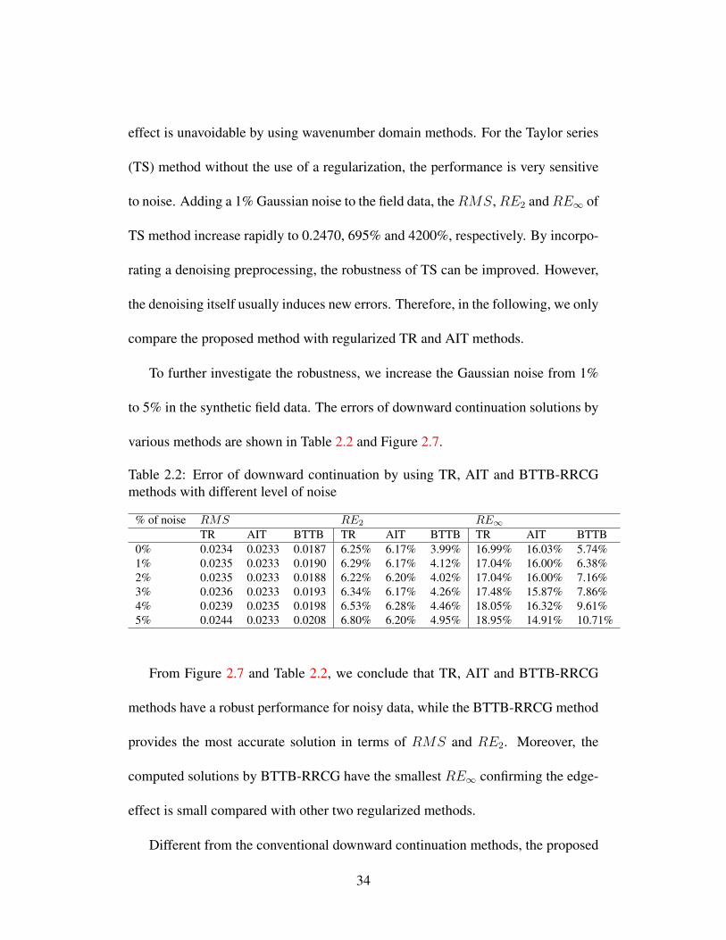
effect is unavoidable by using wavenumber domain methods. For the Taylor series

(TS) method without the use of a regularization, the performance is very sensitive

to noise. Adding a 1% Gaussian noise to the field data, theRMS,RE2 andRE∞ of

TS method increase rapidly to 0.2470, 695% and 4200%, respectively. By incorpo-

rating a denoising preprocessing, the robustness of TS can be improved. However,

the denoising itself usually induces new errors. Therefore, in the following, we only

compare the proposed method with regularized TR and AIT methods.

To further investigate the robustness, we increase the Gaussian noise from 1%

to 5% in the synthetic field data. The errors of downward continuation solutions by

various methods are shown in Table 2.2 and Figure 2.7.

Table 2.2: Error of downward continuation by using TR, AIT and BTTB-RRCG

methods with different level of noise

% of noise RMS RE2 RE∞

TR AIT BTTB TR AIT BTTB TR AIT BTTB

0% 0.0234 0.0233 0.0187 6.25% 6.17% 3.99% 16.99% 16.03% 5.74%

1% 0.0235 0.0233 0.0190 6.29% 6.17% 4.12% 17.04% 16.00% 6.38%

2% 0.0235 0.0233 0.0188 6.22% 6.20% 4.02% 17.04% 16.00% 7.16%

3% 0.0236 0.0233 0.0193 6.34% 6.17% 4.26% 17.48% 15.87% 7.86%

4% 0.0239 0.0235 0.0198 6.53% 6.28% 4.46% 18.05% 16.32% 9.61%

5% 0.0244 0.0233 0.0208 6.80% 6.20% 4.95% 18.95% 14.91% 10.71%

From Figure 2.7 and Table 2.2, we conclude that TR, AIT and BTTB-RRCG

methods have a robust performance for noisy data, while the BTTB-RRCG method

provides the most accurate solution in terms of RMS and RE2. Moreover, the

computed solutions by BTTB-RRCG have the smallest RE∞ confirming the edge-

effect is small compared with other two regularized methods.

Different from the conventional downward continuation methods, the proposed

34

(a) TR (b) AIT

(c) BTTB-RRCG

Figure 2.7: The downward continuation error distribution for 5% noised data by (a)

TR;(b) AIT; (c) BTTB-RRCG method.

BTTB-RRCG method is an iterative method in space domain, which is seldom

investigated due to the computation workload. However, by taking advantage of

the BTTB structure makes the CG type methods as effective as wavenumber domain

methods. Table 2.3 reports the computing time and storage requirement for various

data sizes using the conventional CG method and the BTTB-RRCG method. The

resolution of M ∗N implies that the field data is given by M by N matrix.

Table 2.3: Storage and computing time by conventional and BTTB-RRCG methods

Resolution Conventional CG method BTTB-RRCG

Storage cost Time cost Storage cost Time cost

128*128 1.47 GB 260 seconds 0.31 MB 0.33 seconds

256*256 23.52 GB 1.16 hours 1.22 MB 1.63 seconds

512*512 376.32 GB 18.6 hours 4.95 MB 6.11 seconds

1024*1024 6000 GB 297 hours 30 MB 24.88 seconds

35

From Table 2.3, BTTB-RRCG is much more efficient than the conventional CG.

Moreover, it is noted that as the size of the problem increases, both the computing

cost and storage requirement for the conventional CG increases exponentially. In

contrast, the computational complexity for the BTTB-RRCG increases linearly.

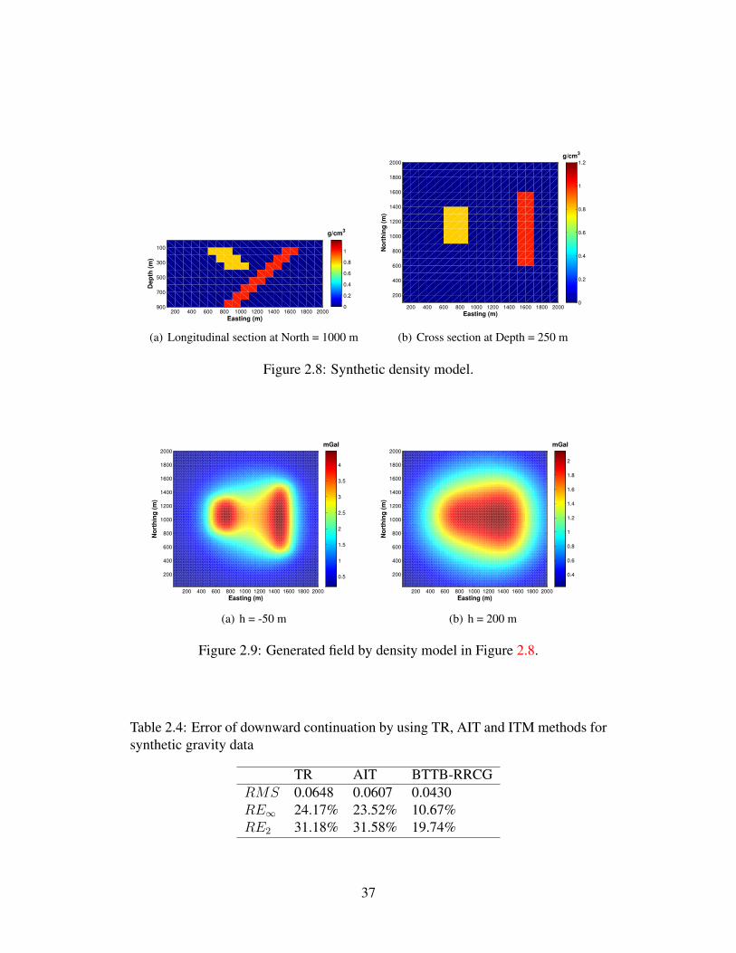
The second synthetic test focuses on the density model as shown in Figure 2.8,

and the gravity field is generated by the synthetic density model. The density model

consists of two dipping prisms underground, where the density of the long prism

and the short prism are 1.0g/cm3 and 0.8g/cm3. The depth from the ground to the

top of the density anomaly is 100 m. The density anomalies are used to generate a

gravity field at h = −50 m and h = 200 m as illustrated in Figure 2.9(a) and 2.9(b)

respectively, where the grid interval is ∆x = ∆y = 20 m. Denote the gravity field

at h = −50 m and h = 200 m by T−50 and T200, we add 2.5% Gaussian noise

to T200 and then apply the TR, AIT and the proposed BTTB-RRCG to conduct the

downward continuation to T200 with continuation distance h = 250 m to compute

the field T−50. The downward continuation is conducted to the underground, be-

cause within the harmonic source-free region, the downward continuation should

be always feasible.

The continuation results are shown in Figure 2.10, and the error distribution is

given in Figure 2.11. By comparing T−50 in Figure 2.10 with T−50 in Figure 2.9(a),

we also report the error in terms of RMS, RE∞ and RE2 in Table 2.4.

From the downward continuation results in Table 2.4, the proposed BTTB-

36

100

300

500

700

900200 400 600 800 1000 1200 1400 1600 1800 2000

Dep

th (

m)

Easting (m)

g/cm3

0

0.2

0.4

0.6

0.8

1

(a) Longitudinal section at North = 1000 m

200 400 600 800 1000 1200 1400 1600 1800 2000

200

400

600

800

1000

1200

1400

1600

1800

2000

Easting (m)

No

rth

ing

(m

)

g/cm

3

0

0.2

0.4

0.6

0.8

1

1.2

(b) Cross section at Depth = 250 m

Figure 2.8: Synthetic density model.

200 400 600 800 1000 1200 1400 1600 1800 2000

200

400

600

800

1000

1200

1400

1600

1800

2000

Easting (m)

No

rth

ing

(m

)

mGal

0.5

1

1.5

2

2.5

3

3.5

4

(a) h = -50 m

200 400 600 800 1000 1200 1400 1600 1800 2000

200

400

600

800

1000

1200

1400

1600

1800

2000

Easting (m)

No

rth

ing

(m

)

mGal

0.4

0.6

0.8

1

1.2

1.4

1.6

1.8

2

(b) h = 200 m

Figure 2.9: Generated field by density model in Figure 2.8.

Table 2.4: Error of downward continuation by using TR, AIT and ITM methods for

synthetic gravity data

TR AIT BTTB-RRCG

RMS 0.0648 0.0607 0.0430

RE∞ 24.17% 23.52% 10.67%

RE2 31.18% 31.58% 19.74%

37

200 400 600 800 1000 1200 1400 1600 1800 2000

200

400

600

800

1000

1200

1400

1600

1800

2000

Easting (m)

No

rth

ing

(m

)

mGal

−1

−0.5

0

0.5

1

1.5

2

2.5

3

3.5

(a) TR

200 400 600 800 1000 1200 1400 1600 1800 2000

200

400

600

800

1000

1200

1400

1600

1800

2000

Easting (m)

No

rth

ing

(m

)

mGal

−0.5

0

0.5

1

1.5

2

2.5

3

3.5

(b) AIT

200 400 600 800 1000 1200 1400 1600 1800 2000

200

400

600

800

1000

1200

1400

1600

1800

2000

Easting (m)

No

rth

ing

(m

)

mGal

0.5

1

1.5

2

2.5

3

3.5

4

(c) BTTB-RRCG

Figure 2.10: The downward continuation results by (a) TR;(b) AIT; (c) BTTB-

RRCG method.

200 400 600 800 1000 1200 1400 1600 1800 2000

200

400

600

800

1000

1200

1400

1600

1800

2000

Easting (m)

No

rth

ing

(m

)

mGal

−1.5

−1

−0.5

0

0.5

1

1.5

(a) TR

200 400 600 800 1000 1200 1400 1600 1800 2000

200

400

600

800

1000

1200

1400

1600

1800

2000

Easting (m)

No

rth

ing

(m

)

mGal

−1.5

−1

−0.5

0

0.5

1

1.5

(b) AIT

200 400 600 800 1000 1200 1400 1600 1800 2000

200

400

600

800

1000

1200

1400

1600

1800

2000

Easting (m)

No

rth

ing

(m

)

mGal

−1.5

−1

−0.5

0

0.5

1

1.5

(c) BTTB-RRCG

Figure 2.11: The downward continuation error distribution for by (a) TR;(b) AIT;

(c) BTTB-RRCG method.

38

RRCG method is clearly more accurate than the TR and AIT method in terms of

RMS, RE∞ and RE2. More importantly, consider that for the density model in

Figure 2.10, all anomalies are positive which means generated gravity fields should

be positive. However, in Figure 2.10, both TR and AIT methods induce negative

values on the left side. However, the proposed BTTB-RRCG scheme perfectly p-

reserve the positivity property, and has a much smaller boundary effect than other

two methods.

2.4 Applications using real field data

Now, we apply the proposed BTTB-RRCG scheme using real field data 1. The field

data shown in Figure 2.12(a) is the magnetic field distribution at the ground level,

where the data grid size are ∆x = ∆y = 10 m. The upward continuation of the

field data to h = 200 m is shown in Figure 2.12(b),

(a) h=0 m (b) h = 200 m

Figure 2.12: (a) The real magnetic field data at h = 0 m;(b) The upward continua-

tion by ∆ = 200 m of the field data in Figure 2.12(a)

1The field data used in this thesis is provided by TerraNotes Ltd

39

By adding 2.5% Gaussian noise to the potential field in Figure 2.12(b), the TR,

AIT and BTTB-RRCG methods are used for a downward computation with a con-

tinuation distance h = 200 m. The same regularization parameter for the synthet-

ic data is used for the real field data applications. In real applications, the exact

downward continuation results are always unknown, therefore we can only have an

estimation of the value for the optimal regularization parameters. In our study, we

use the optimal regularization parameters obtained in the synthetic case for the real

field data. Recall that in a downward continuation formulation (2.1.10), the upward

continuation operator A depends only on the ∆x,∆y, and h. Once these parameters

are fixed, the spectral characteristic of the continuation operator is determined. In

the first synthetic case, ∆x = ∆y = 9.98m, and h = 200m, while in the real field

data, ∆x = ∆y = 10m, and h = 200m, which means that the spectral characteristic

of the continuation operators are similar between the first synthetic case and real

field case.

The downward continuation results for the real field data are shown in Figure

2.13, and their error distributions are illustrated in Figure 2.14.

From Figure 2.14(a) and 2.14(b), we observe that the edge-effect is evident n-

ear the boundary for the TR and AIT methods. A simple procedure to improve

the computed solution is to remove a layer near the boundary. Figures 2.15 and

2.16 illustrate the solutions by tailoring 40 grids (i.e., 400 m) from the edge for the

solutions shown in Figure 2.13 and 2.14. It is important to note that the solution

40

(a) TR (b) AIT

(c) BTTB-RRCG

Figure 2.13: The downward continuation by ∆h = 200 m for 2.5% noised real field

data by (a) TR;(b) AIT; (c) BTTB-RRCG method.

(a) TR (b) AIT

(c) BTTB-RRCG

Figure 2.14: The downward continuation error distribution for 2.5% noised real

field data by (a) TR;(b) AIT; (c) BTTB-RRCG method.

41

computed by the BTTB-RRCG method is very stable and with little edge effec-

t. The BTTB-RRCG scheme is an accurate scheme even without the use of any

extrapolating and tailoring process.

(a) TR (b) AIT

(c) BTTB-RRCG

Figure 2.15: The downward continuation by ∆h = 200 m after tailoring for 2.5%

noised real field data by (a) TR;(b) AIT; (c) BTTB-RRCG method.

From the tailored computed solutions for downward continuation shown in Fig-

ures 2.15 and 2.16, it is clear that the BTTB-RRCG method is robust and accu-

rate for the real field data compared with TR and AIT methods. By evaluating

downward continuation results by TR, AIT and BTTB-RRCG methods in terms of

RMS, Table 2.5 reports the errors in terms of L2 and L∞ norm. Figure 2.17 dis-

plays the convergence rate of the BTTB-RRCG using real field data. It is noted

that the residue reaches a steady state after 15 iterations, hence the iteration can be

42

(a) TR (b) AIT

(c) BTTB-RRCG

Figure 2.16: The downward continuation error distribution after tailoring for 2.5%

noised real field data by (a) TR;(b) AIT; (c) BTTB-RRCG method.

terminated much earlier than the prescribed 35 iterations.

Table 2.5: Error by TR, AIT and BTTB-RRCG methods for real field data

TR AIT BTTB-RRCG

RMS 0.0348 0.0357 0.0240

RE2 3.39% 3.55% 1.61%

RE∞ 6.02% 6.52% 3.37%

The robustness and accuracy of the proposed BTTB-RRCG method are verified

by the simulation results based on test cases using synthetic and field data. The CG

type method is a popular iterative technique for solving large scale linear equations,

and it is particularly efficient for large sparse matrices. The main computational

work per iteration is typically depended on the matrix-vector product operation. In

the present applications, the matrix A is a full matrix, and without taking advantage

43

0 5 10 15 20 25 30 350.4

0.6

0.8

1

1.2

1.4

1.6

1.8

2

Number of iteration

log

10(e

)

Figure 2.17: Convergence rate of BTTB-RRCG method in the real field data appli-

cation, where e = ||ATh − T0||2.

of BTTB structure, it requires considerable computing resources. We compare the

computational complexity using the conventional RRCG method and the BTTB-

RRCG method. The results speak for itself. It is clear that the utilizing the BTTB-

structure dramatically reduces both the storage and computing cost, and a large

scale downward continuation problem can be computed with a modest computing

resource.

2.5 Conclusion

In this chapter, we propose efficient approach by utilizing the BTTB structure with

the re-weighted regularized conjugate gradient method. Not only the BTTB struc-

ture greatly enhance the stability and robustness of the downward continuation com-

putation, but the computation workload and storage requirement are also signifi-

cantly reduced. We demonstrate that compared with the conventional wavenumber

domain FFT-based methods, the BTTB-RRCG scheme induce negligible artifac-

t near the boundary. The simulation results using the clean and highly perturbed

44

synthetic field data as well as the real field data verify that the proposed method are

more accurate and robust compared to the Taylor-series and wavenumber domain

regularized methods.

It is also easier to implement various regularization stabilizers directly in time

domain instead of wavenumber domain. By plotting the residue at each iteration,

we can quickly estimate the number of iterations required for the BTTB-RRCG

method. The BTTB structure allows the design of an optimal preconditioner to

further accelerate the convergence rate, in which the preconditioner is also in the

form of BTTB matrix.

The work presented in this chapter has been published in Journal of Applied

Geophysics [121].

45

Chapter 3

Numerical Inversion for Magnetization

Magnetic field survey is a popular tool for fast mapping of large areas in geophysical

and environmental study. A typical survey consists of mapping one or more com-

ponents of the earth geomagnetic field in order to analyze the magnetic anomalies.

The magnetic anomalies mapping is generally used in many geological applications

such as estimating the basement topography, assessing the depth in oil exploration

and the magnetic polarization in mineral prospecting.

Recall that for the potential field inversion problem, the model can be expressed

mathematically as an integral formulation, which can be converted into linear equa-

tions Au = b, where b is the observation magnetic field data, and the matrix A is

often large, dense and ill-conditioned [29].

Instead of using a 3D potential field inversion [64, 82], 2-D model is more

preferred in many cases, and this is particularly true for the aero-magnetic survey.

The simplicity of a 2-D model also makes the 2-D inversion practical and efficient.

The inversion for tabular magnetic anomalies or thin layer magnetic anomalies have

been investigated in [40, 87, 6, 88, 111].

For an irregular raw data, it can be rewritten into a uniform data conveniently by

46

the use of a regridding procedure. Many efficient methods have been developed, for

instance, Briggs [10] proposed a minimum curvature method for regrid non-uniform

data. Cordell and Blakely [25, 9] presented an equivalent layer method (ELM), in

which a fictitious source layer is introduced, and then the non-uniform data points

are interpolated on a uniform grid according to the source layer. The advantage of

implementing the ELM has been reported by Cooper [23], and a comparative study

of ELM and the minimum curvature method can be found in [70].

Once the field data are gridded regularly, the linear system of a magnetic in-

version problem leads to a symmetric Block-Toeplitz Toeplitz-Block (BTTB) ma-

trix, which has a similar form as the downward continuation problem discussed in

Chapter 2. Actually, in the study of interpolating the potential field data, the BT-

TB structure has already been noticed. Rauth and Strohmer [89] investigated the

potential field gridding problem by interpolating the non-uniform field data into a

uniform field data, where a trigonometric polynomial is used to approximate the

magnetic field, and the coefficients of the polynomial are computed by solving a

BTTB system.

In this chapter, we investigate fast magnetic field inversion scheme. Particu-

lar attention is focused on incorporating the BTTB structure to develop efficient

numerical inversion algorithms based on the multigrid (MG) technique. A com-

parative study of the MG and conjugate gradient type methods is presented, and

the performance of these methods is validated by numerical simulations applied to

47

the synthetic field data and the real geophysical data. We show that the BTTB-MG

technique is robust, accurate, and compared with regularized methods, it is provides

more information.

3.1 Magnetic Field Forward Model

Assuming that the magnetic data covers an area which is filled with a set of vertical

prisms with arbitrary horizontal section and the bottom at infinity, the magnetic

anomaly reduced to the pole is given by a layer of poles on the top of each prism as

shown in Figure 3.1.

Figure 3.1: Forward Model.

The magnetization is defined as the magnetic moment (M) per volume given by

J =dM

dv, (3.1.1)

which is induced by the earth magnetic field, and it is the source of the magnetic

48

anomaly. To determine the magnetic field generated by magnetization, the concept

of magnetic scalar potential ψ is introduced. When there is no free current, the

magnetic scalar potential can be used to determine the magnetic H-field especially

for the permanent magnets in the following way:

H = −∇ψ. (3.1.2)

It is known that the magnetic potential generated by dM at an arbitrary point P

is defined by dψ = dM·rρ

, where r is a coordinate of P , and ρ is the distance from P

to dv. According to (3.1.1),

dψ = −[

J · ∇(1

ρ)

]dv. (3.1.3)

Thus, the magnetic potential at the point P generated by a prism is given by

ψ = −∫

V

[J · ∇(

1

ρ)

]dv. (3.1.4)

According to the Gauss formula, (3.1.4) can be further rewritten as

ψ =

∫

S

(J · dS)ρ

−∫

V

(divJ

ρ)dv. (3.1.5)

where V is the volume of magnetization, and S is the surface area of the magne-

tization. By assuming that in each prism, the value of magnetization J is uniform,

and the magnetization in the prisms have the same direction, then divJ = 0, and

only the first term in (3.1.5) is retained. The integral on the side facing the prisms

can be neglected, since the bottom is assumed to be infinitely deep and the upper

49

surface can be regarded as the source plane. Hence, (3.1.5) can be simplified as

ψ =

∫

S

JnρdS, (3.1.6)

where Jn is the vertical magnetization in the nth prism. Here, the magnetic potential

ψ is a function of the coordinate point P . If we denote the position of dv as Q, and

the coordinate Q as r′, then ρ = |r − r′|. According to (3.1.2), the magnetic field

generated by each prism is given by

H = −∇ψ = −∇∫

S

Jn|r − r′|dS, (3.1.7)

in which the vertical magnetic field is

Hz =

∫

S

Jn(z − z′)

|r − r′|3 dS. (3.1.8)

Now, consider all prisms as a whole, thus the magnetic field at the point P

is generated by all prisms. By (3.1.8), denote the Jn as a function of coordinate,

then the magnetic anomaly is described by the convolution of two functions: the

kernel depending on the positions of the observations and the other describing the

distribution of magnetization as the following:

Hz(x, y, z) =

∫∫

S

m(x′, y′, z′)G(x, y, z, x′, y′, z′)dx′dy′, (3.1.9)

where

G(x, y, z, x′, y′, z′) =z − z′

[(x− x′)2 + (y − y′)2 + (z − z′)2]3

2

. (3.1.10)

50

It is interesting to note that the kernel in (3.1.10) has exactly the same format as

that in Chapter 2 of a downward continuation formulation. Similarly, the forward

model of a magnetic field problem can be written as

b = Au, (3.1.11)

where b is the observed magnetic field, u is the magnetization distribution, and A

is the magnetic forward operator.

3.1.1 Multigrid techniques

It is well-known that the convergence of CG type methods depends on the condi-

tion number of the matrix A. In a magnetic inversion problem, the system matrix in

(3.1.11) is usually very ill-conditioned and with a large condition number. Multi-

grid (MG) technique is developed based on multilevel iterative methods, and it has

generally been regarded that MG is an optimal iterative method for solving large

positive definite systems resulting from elliptic partial differential equations. The

technique is optimal since the convergence rate is independent of the condition

number of A and the size of the linear system.

When solving a linear system by a classical relaxation scheme based on the

Jacobi or Gauss-Seidel method, we note that the high frequency error can be elimi-

nated very quickly, but it is hard to remove the low frequency error. Consequently,

a rapid error reduction is typically observed at the initial stage, and after that the

51

error decreases very slowly leading to a slow convergence rate.

Suppose we want to solve a linear system (3.1.11), instead of applying an iter-

ative scheme directly, we now consider the solution being computed by applying a

relaxation scheme to multilevel or multigrid systems

Ajuj = bj, (3.1.12)

where Aj denotes the matrix at different grid levels with A1=A known as the finest

grid, and the matrices Aj , j = 2, 3, · · · are referred as the coarse grid levels, bj and

uj are the observed field and inverted solution in each level. The coefficient matrix

Aj for j > 1 can be constructed using the same way as for A1 but with a coarser

mesh. The superior performance of a MG method is achieved due to the fact that

the low frequency error on the fine grid can be regarded as the high frequency error

on the coarse gird. Thus by employing a relaxation scheme to a sequence of various

grid levels, the high and low frequency error components can be eliminated rapidly

and this ensures a fast convergence rate for a MG method.

The idea of a MG approach can be easily explained by a two-grid method as

illustrated in Figure 3.2.

Figure 3.2: Two-grid and V-cyle MG.

52

Recall that if u is the computed solution of Au = b, the residual is defined by

r = b − Au = A(u − u) = Ae, (3.1.13)

where e is the error vector. By solving Ae = r, we can then improve the numerical

solution, such that

u = u + e. (3.1.14)

Let Ω1 and Ω2 denote the fine grid (i.e. level 1) and the coarse grid (i.e. level

2). In a two-grid method, starting with an initial approximation u0, the algorithm is

given as

(i) Smoothing step: In Ω1, apply relaxation (3.1.15) v1 time, u1 → S(u1, b1),

(ii) Compute the residual and transfer from Ω1 to Ω2:

r1 = b1 − A1u1, r2 = R21r

1,

(iii) In Ω2, solve the error equation: A2e2 = r2,

(iv) Interpolate error from Ω2 to Ω1 and improve the approximation: u1 → u1 +

I12e2,

(v) Correction step: Apply relaxation again v2 time, u1 → S(u1, b1),

(vi) Repeat the procedure until a stopping criteria such as ||r1|| < ε is achieved.

Here, S(u1, b1) denotes a smoothing or a relaxation process which will be de-

fined shortly. Dropping the superscript index for the matrix A, let A = D−L−LT,

53

where L is the lower triangular of matrix A, u0 is an initial approximation, the

weighted Jacobi relaxation is selected as a smoothing operator such that S(u1, b1)

is defined by

u1 = [(1− ω)I + ωD−1(L + LT)]u0 + ωD−1b1, (3.1.15)

where ω is a parameter, which can be estimated by a formula proposed in [100]:

ω ≤ a0,0ρ(A)

, (3.1.16)

where a0,0 is the first element of the matrix A and ρ(A) is the spectral radius of A.

Note that R21 is a restriction operator which is used to transfer the residual from a

fine grid denoted as grid 1 to coarse grid denoted as grid 2, and I12 is an interpolation

operator which is used to interpolate the error from a coarse grid to a fine grid. Also,

(i) is generally referred as the smoothing step, and (iii) is the correction step in an

MG cycle.

The most important advantage of using BTTB structure in the multi-grid method

is that, in step (iii), the system matrix of at coarser level always keep the BTTB

structure as the original system. This means that in each level, we are able to apply

the efficient FFT to accelerate the computation. By repeatedly applying a two-grid

method, we can construct an efficient multigrid method, and the V-cycle MG is

shown in Figure 3.2. The details on the construction of the coarse grid coefficient

matrices, the restriction and interpolation operators can be found in [11].

54

3.2 Numerical Simulations

To validate the effectiveness of the proposed BTTB-MG scheme, we consider the

following test cases. The proposed BTTB-MG method will be assessed and com-

pared with the BTTB-RRCG method based in terms of efficiency, accuracy and

robustness. The computation is carried out using a laptop computer with Intel i7-

3632QM 2.2 Hz and 12G RAM. For the MG method, the level of grids in the

V-cycle will be determined, and v1 =v2 = 1 will be used in the smoothing and

correction steps.

3.2.1 Synthetic data

The first test case is constructed as in Figure 3.3, which illustrates an initial mag-

netization distribution. The reason we use this synthetic data has been discussed

in Chapter 2, and it is considered to be the source generating the magnetic field

solution for the magnetic inversion problem. In Figure 3.4, we display the comput-

ed magnetic field data generated by the given synthetic magnetization distribution

with different depth h = 50m, 100m, 200m, 250m, respectively. By applying the

magnetic inversion scheme to these synthetic magnetic field data, we can evalu-

ate the performance of the BTTB-MG scheme, and compare it with the proposed

BTTB-RRCG scheme. First, let the relative error (RE) be defined as:

RE =||Uinv − Uexact||∞

||Uexact||∞× 100%, (3.2.1)

55

Table 3.1: Condition number of the coefficient matrix corresponding to different

depths.

Depth (m) Condition Number

50 1.2410*108

100 5.8372*108

200 2.1781*109

250 3.2852*109

where Uinv is the computed inverse solution, Uexact is the exact solution.

Figure 3.3: Initial magnetization distribution.

In Table 3.1, we list the condition number of the coefficient matrix T in (3.1.11)

for a range of depths from h = 50 m to 250 m. The condition number increases as

the depth is increasing, therefore, within the 250 m depth, that the largest condition

number appears at the maximum depth. Hence, the synthetic field data at h = 250

m is chosen as the test case in which the simulation data will be inverted. Instead

of using fixed iteration numbers as in Chapter 2, the stopping criterion used in this

56

Figure 3.4: Magnetic field data at different depths.

computation is

||rn||∞||r0||∞

< tol,

where tol is the tolerance of the iteration, rn is the residue at the n-step iterations,

r0 is the initial residue. For the multigrid method, to determine the optimal level of

the grid in V-cycle iteration scheme, we report the level of grids vs the computing

time and number of cycles in the following Table 3.2.

Table 3.2: Computing time and number of V-cycles of MG with various grid levels.

Tol=10−3 Tol=10−4

Level TMG (s) N TMG (s) N2 7.122357 24 62.540190 203

3 3.575487 11 32.270307 97

4 3.248739 10 33.257580 103

5 3.209048 10 33.601279 103

57

In Table 3.2, we present the MG results where the level denotes the number of

grid levels used in a V-cycle, T is the computing time in second, N is the number

of cycles to reach a given tolerance. It is clear that a good performance is achieved

when the grid level is greater than two. However, for the inversion problem consid-

ered here, taking three grid levels in a V-cycle seems to suffice, and a 50% reduction

in computing time over a two-grid method is achieved. However, it should be noted

that the number of multigrid levels is problem dependent and also depends on the

resolution of grids. We use three level grid in the following problem because the

field data used in the simulation has very similar resolution with the case we tested

above. While for the data with different resolution, more work is needed to find the

optimal grid level.

To compare the effectiveness of various numerical inversion schemes, Table 3.3

reports the inversion of the synthetic magnetic field data at h = 250 m by CG,

Preconditioned CG (PCG), RRCG and MG methods, where all numerical schemes

are taking advantage of the BTTB structure. Particularly, the preconditioner used in

the PCG method is constructed according to (4.2.9) in Chapter 4. Here, N denotes

the number of iterations in CG type methods and the number of cycles in MG

method, and N/A means that the scheme fails to converge within 2000 iterations. In

Figure 3.5, we plot the convergence rate for the CG, PCG, RRCG and MG methods.

From the results presented in Table 3.3 and Figure 3.5, we note that the pre-

58

Table 3.3: Computing time and iteration numbers of various numerical inversion

for synthetic data at h=250m.

Tolerance TCG (s) N TRRCG (s) N TPCG (s) N TMG (s) N

1 ∗ 10−2 0.678969 9 9.323636 50 0.547881 7 0.585323 2

1 ∗ 10−3 1.330730 19 31.220969 167 1.175903 14 3.219449 11

1 ∗ 10−4 3.477457 53 N/A N/A 2.692719 35 27.853854 97

1 ∗ 10−5 11.896358 182 N/A N/A 7.668079 99 306.236100 1026

conditioned CG (PCG) is the most efficient in term of computing time needed to

reach a given accuracy, and it then follows by the CG, MG and RRCG. Although

the RRCG method has been a robust method used in many geophysical application-

s, it has a slow convergence rate and fails to reach a given tolerance within 2000

iterations when a small tolerance is required as indicated in Table 3.3. When the

tolerance is in the level of 1∗10−2 or 1∗10−3, the performance of the CG, PCG and

MG are comparable in terms of convergence rate and the computing time required.

In Figure 3.6, the computed solutions of the four methods for the inversion problem

are displayed.

In Table 3.4, we present the relative errors between the accurate distribution and

the inversion solution computed by the CG and MG methods for the test cases using

the synthetic data. For a given depth, the relative error can be reduced by setting a

smaller tolerance. It is observed that for a fixed tolerance, the error increases as the

depth is increasing.

The test cases investigated here are constructed based on synthetic data, and

they are essentially noise-free data. However, the accuracy and effectiveness of an

inversion algorithm can not be guaranteed if the data is contaminated with noise. In

59

Table 3.4: Relative error of CG and MG method at different depths and tolerance.

CG MG

Depth (m) 10−2

10−3

10−4

10−5

10−2

10−3

10−4

10−5

50 6.55% 2.83% 1.30% 0.52% 6.72% 4.32% 2.13% 1.75%

100 11.54% 3.55% 2.33% 0.97% 14.00% 9.77% 5.09% 3.70%

200 21.78% 14.95% 8.62% 6.7% 24.11% 16.47% 10.43% 7.75%

250 24.42% 19.28% 12.97% 6.67% 27.20% 21.25% 15.00% 9.87%

0 20 40 60 80 100 120 140 160 180−1.5

−1

−0.5

0

0.5

1

1.5

2

2.5

Number of iteration

log

10 o

f re

sid

ua

l

CG

PCG

RRCG

MG

Figure 3.5: Convergence rate of CG, RRCG, PCG and MG method at tolerance=1∗10−3.

Figure 3.6: Inversion of the magnetic field at h=250 m by CG, RRCG, PCG and

MG method.

60

reality, the magnetic field data obtained by measurement are always contaminated

with noise. Thus, it is important to study the robustness of numerical inversion

schemes.

Let A be the potential field resulted from a synthetic magnetization distribution,

and E be the matrix with coefficients generated randomly in the range [0, 1] drawn

from the standard normal distribution. Considering the noise in the observation data

is caused from the measuring apparatus, the noisy observation data A with a noise

level of α% can be defined by A = A + α% ∗ E.

In Table 3.5 and Figure 3.7, the performance of the CG, PCG, RRCG and MG

methods are compared when the observation data with different level of noise are

inverted. When the noise level is 0%, the test case converts to the original clean

synthetic magnetic field data. It is observed that although the CG and PCG are very

effective when applied to clean data, their performances deteriorated rapidly when

noise is added in the field data. The RRCG is a very reliable method, and the rel-

ative error remains almost at the same level even when a 20% noise is introduced.

The MG method is not sensitive when the noise level is less than 10%, but the noise

effect becomes noticeable when the noise level is greater than 10%. Unlike the R-

RCG, a regularization procedure is not incorporated to the MG method. Therefore,

the performance could be improved if a suitable regularization is introduced.

From the computational results presented for the synthetic data, it is clear that

both CG and PCG methods are sensitive to the noisy data, thus the methods can not

61

Table 3.5: Relative error of CG, RRCG, PG and MG with different noise levels (%).

0% 1% 4% 8% 12% 16% 20%

CG 24.42% 24.46% 24.25% 26.13% 4.8*104 6.7*104 8.0*104

RRCG 26.51% 26.51% 26.40% 25.63% 25.34% 25.00% 24.09%

PCG 25.80% 60.36% 7.2*106 1.4*107

MG 27.20% 27.19% 27.24% 26.60% 27.78% 29.49% 32.90%

0 1 4 8 12 16 2020

30

40

50

60

70

80

90

100

Noise level(%)

Re

lative

err

or(

%)

CG

RRCG

PCG

MG

Figure 3.7: Error vs noise level for the CG, RRCG, PCG and MG method under

tolerance=10−2.

62

be used for real field data. The proposed BTTB-MG and BTTB-RRCG methods

are more robust than the CG and PCG methods. However, the BTTB-MG method

is non-regularized, and is more accurate in term of relative error.

3.2.2 Real Data

Given a real geophysical data, the numerical inversion program provides an estimate

of magnetization of underground rocks at certain depth h. Generally speaking, h

is an unknown, and by producing a sequence of magnetization at various depths, it

would provide useful information for the geologists or geophysicists to interpret the

computation results and to study how dependent the results are on the variations of

h.

In order to reduce the numerical artifact introduced by the numerical scheme

near the boundary, we adjust the results presented in the window shown in Figure

3.8 which is obtained by removing the shadow layer from the original data. Note

that the shadow layer has a thickness of only five grid points, and the original data

field usually covers several hundred grid points in both directions.

3.2.2.1 Test case I

For the first test case, the magnetic field data covers a square area with 6000m in

both the x- and y- directions, and the interval between each grids is 12m. Thus the

resolution of the magnetic field data is 500 by 500 as shown in the Figure 3.9.

63

Figure 3.8: Original field data and selected window W.

Figure 3.9: Test case I.

64

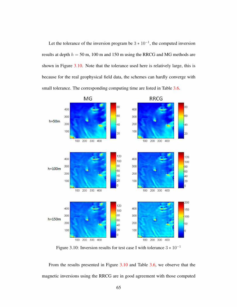
Let the tolerance of the inversion program be 3 ∗ 10−1, the computed inversion

results at depth h = 50 m, 100 m and 150 m using the RRCG and MG methods are

shown in Figure 3.10. Note that the tolerance used here is relatively large, this is

because for the real geophysical field data, the schemes can hardly converge with

small tolerance. The corresponding computing time are listed in Table 3.6.

Figure 3.10: Inversion results for test case I with tolerance 3 ∗ 10−1

From the results presented in Figure 3.10 and Table 3.6, we observe that the

magnetic inversions using the RRCG are in good agreement with those computed

65

Table 3.6: Computing time for test case I with tolerance 3 ∗ 10−1

Depth (m) TRRCG (s) TMG (s)

50 1.102995 0.466652

100 2.121059 0.964995

150 3.515279 1.404609

by MG. At h = 50 m, the two results are almost identical. However, as h in-

creases, the RRCG produces noticeable artifacts near the boundary. To investigate

the sensitivity of the RRCG and MG methods to the given tolerance, we carry out

the simulation with fixed depths, namely h=50 m and h=100 m, and examine the

inversion solutions at two values of tolerances. Figure 3.11 and 3.12 present the

numerical inversion results, and the corresponding computing time are reported in

Table 3.7. As expected, the computed solutions are less sensitive when h is small

as shown in Figure 3.11. Figure 3.12 displays the RRCG and MG results when

h = 100 m and the tolerances are set at 4 ∗ 10−1 and 2 ∗ 10−1, respectively. Here,

the difference between the inversion results corresponding with two tolerances are

obvious. Moreover, the artifacts resulting from RRCG at ε = 2 ∗ 10−1 is also no-

ticeable. From the computing time reported in Tables 3.6 and 3.7, it is clear that

MG is more efficient and requires less computing time than the RRCG for all cases

tested.

Table 3.7: Computing time for test case I using RRCG and MG

Depth (m) Tolerance TRRCG (s) TMG (s)

50 ε = 4 ∗ 10−1 0.894744 0.304539

50 ε = 2 ∗ 10−1 2.557688 0.964625

100 ε = 4 ∗ 10−1 1.576802 0.549794

100 ε = 2 ∗ 10−1 4.114992 2.068582

66

Figure 3.11: Inversion result for test case I at depth h=50 m

3.2.2.2 Test case II

In the second test case, the real magnetic field data is given as a rectangle area with

length=14040 m, width=8720 m, and the interval between each grids is 20 m. The

real magnetic field is defined by a two-dimensional grid of 702 by 436 as shown in

Figure 3.13.

To further evaluate the two numerical inversion schemes, Figure 3.14 presents

the computed solutions using RRCG and MG methods at a fixed depth h=100m

for tolerance 1 ∗ 10−1, 5 ∗ 10−2 and 1 ∗ 10−2. In Figure 3.15, the inversion results

at various depths h=50 m, 100 m and 150 m are illustrated. The computing time

67

Figure 3.12: Inversion result for test case I at depth h=100m

required by the two methods are reported in Table 3.8.

From the results applied to test case II, we note that when the depth h is small,

the inversion results produced by RRCG and MG methods are very similar. Howev-

er, the discrepancy in terms of the maximum and minimum recovered magnetization

become noticeable as the depth increases and when the tolerance is decreasing. It

is noted that both methods are capable of capturing similar underground geological

features, but the RRCG produces larger artifacts near the boundary. The superior

performance of the MG method over the RRCG is also clearly demonstrated by the

significant saving in computing time as shown in Table 3.8.

Recall that in Chapter 2, we have shown that the BTTB-RRCG method produces

68

Figure 3.13: Test case II.

Table 3.8: The computing time for test case II.

Depth (m) Tolerance TRRCG (s) TMG (s)

100 ε = 1 ∗ 10−1 2.626800 0.700371

100 ε = 5 ∗ 10−2 8.858662 2.744200

100 ε = 1 ∗ 10−2 144.395461 46.382697

50 ε = 1 ∗ 10−2 33.221171 15.612463

200 ε = 1 ∗ 10−2 352.861550 75.893122

69

Figure 3.14: Inversion result for test case II at h = 100m.

70

Figure 3.15: Inversion result for test case II with tolerance = 1 ∗ 10−2.

71

much smaller edge-effect than the wavenumber domain method. However, applying

to the same field data, proposed BTTB-MG method has a smaller edge-effect than

the BTTB-RRCG method even when a small tolerance is applied. On the other

hand, for the field data with modest noise level, the BTTB-MG method is as stable

as BTTB-RRCG method.

It should be noted that when the noise level is high, the regularization should

be used, and the BTTB-MG method can also be implemented by incorporating the

regularization stabilizers.

3.3 Concluding Remarks

In this chapter, efficient multi-grid inversion schemes for magnetization inversion

is developed. It is important to recognize that the inversion results can be computed

by solving a symmetric Block-Toeplitz Toeplitz-Block (BTTB) system. The linear

system is frequently large, dense and ill-conditioned. Direct implementation of the

matrix coefficients will require considerable storage and leading to the requirement

of large computing resources for the solution. By taking advantages of a symmet-

ric BTTB property, the storage requirement can be reduced from O(N2) to O(N)

and the computational work for a typical iterative scheme decreases to O(N logN)

instead of O(N2). Therefore, efficient numerical inversion schemes can be devel-

oped, and they are capable of dealing with a large scale inversion problem.

It has been demonstrated that the RRCG and MG methods are effective numer-

72

ical tools for the inversion problems. Both methods have been tested to problems

generated by synthetic data and real magnetic field data. Based on the numeri-

cal simulation, we conclude that for the field data with moderate perturbation, the

BTTB-MG technique has a superior performance compared to the BTTB-RRCG

method, in particular, the artifact near the boundary resulting from BTTB-MG is

much less than that produced by the BTTB-RRCG. Moreover, significant saving in

computing time is achieved by the BTTB-MG for all cases tested in this paper.

As a powerful structure in geophysical problem, the BTTB structure can be gen-

eralized to the 3D inversion problems, which will be discussed in the next chapter.

The work reported in this chapter has already been published in International

Journal of Numerical Analysis and Modeling [120].

73

Chapter 4

3D Inversion for Gravity Field Data

Gravity field survey is an essential step in prospecting of large areas in geophysical

and environmental study. In many applications, meaningful underground informa-

tion can be obtained from the density distribution. Similar to the magnetic field,

inversion can be used to deduce the density from the observation gravity field, and

the inversion solution is then sought by repeatedly computing the underground den-

sity according to the observation gravity. Unfortunately, there exists some structures

producing a zero external gravity field. Therefore, for a given field data, there are

infinite underground models generating exactly the same field. Hence, it is impos-

sible to seek an exact solution from an inversion process. However, using prior

information and/or applying regularization, we can obtain meaningful information

from the observation.

In general, two techniques are commonly used for the three-dimension inversion

schemes. The first one is based on the structural inversion, in which the structure in-

formation is obtained from inversion results, such as the Euler deconvolution [104],

wavelet analysis [50], signal analysis [91, 7] and so on. The structural inversion

techniques also include using models with certain properties such as inversion for

74

tabular anomalous [40, 87, 6, 88, 111], inversion for interfacing surface or anomaly

boundaries [95, 83, 85].

The other technique is the generalized inversion based on discretizing the 3D

underground into cells with constant susceptibility or density. To guarantee a u-

nique solution, regularization or prior information should be incorporated. In par-

ticular, a smoothness regularization [64, 65] can be employed to produce a smooth

inversion solution, whereas a focusing regularization [84, 125, 122, 124] is appro-

priate for a compact solution. The inversion solution largely depends on which

stabilizer is used, but it may not be consistent with the real geological features. In

some applications, adding prior information from previous experience or borehole

data can result in certain geologic constraints [60]. To reduce the uncertainty in the

inversion solution, cell-based inversion methods utilizing the assumption of certain

physical property have been reported [12, 58]. For large scale potential field da-

ta, 3D inversion computation is a very challenging task and the solution requires

significant computer resource. Hence, it is desirable to develop efficient numerical

inversion schemes so that the solution can be computed rapidly with modest com-

puting time and storage requirement. Recently, wavelet based methods [66, 29]

have been considered to compress the sensitivity matrix by dropping small wavelet

coefficients. Similar work includes the foot-print technique [26, 126], in which the

threshold value to the sensitivity matrix is defined by users. Both wavelet method

and moving foot-print technique aim at representing a dense matrix by a sparse ma-

75

trix. They can be applied to data domain and model domain [84, 4, 29, 46, 30]. In

addition, down-sampling in data domain and model domain can further reduce the

computation load with a cost of lowering the resolution of the inversion solution.

Compared with the 2-D problem in Chapters 2 and 3, a 3-D inversion produces a

much larger system with dense and ill-conditioned matrix. The storage requirement

of 3-D problem is of order O(n2) and computational work per iteration of O(n2),

while the n in 3-D can be significantly larger than that in 2-D problem. However, the

computational complexity can be dramatically reduced from O(n2) to O(n log n)

by using FFT based methods for regular field data. Pilkington applies a 2D Fourier

transform for the 3-D magnetic field inversion. A 3-D Fourier transform method

for the potential field inversion is also reported [13]. As discussed before, for an ir-

regular or non-uniform data, fast gridding algorithms [10, 25, 9, 23] are available to

convert irregular data into regular data, and the computational complexity is O(n).

In this chapter, we propose a novel numerical scheme based on a 2-D multi-layer

model for a 3-D gravity field inversion. The consistency and convergence are stud-

ied, and an error estimate is derived. Unlike the previous FFT-based schemes where

FFT is applied to the kernel, the present scheme is directly applied by discretizing

the proposed mutli-layer model in the space domain, such that a BTTB structure

is obtained. Moreover, the FFT is employed by embedding the BTTB matrix into

a BCCB matrix. The BTTB-based scheme has attractive features in constructing

preconditioning operator and regularization. Differed from the popular Conjugate

76

Gradient (CG) inversion scheme reported by Pilkington [82] utilizing a simple pre-

conditioner in the form of diagonal matrix, the preconditioner presented here is

optimal and it is in the form of BCCB matrix. Using recent mathematical results

and properties related to BCCB and BTTB structures, optimal preconditioned CG

solver can be accelerated by FFT, and a good convergence rate can be achieved. We

also incorporate the regularization into the BTTB framework. To the best of our

knowledge, the application of FFT for a general stabilizer have not been reported.

For a large scale 3-D inversion problem, the computation time usually can not

be predetermined until the whole inversion is completed. In our work, numerical

analysis including the convergence order of the computational scheme is presented.

Useful information can then be extracted by carrying out inversions with various

resolutions, and a reasonable computing time can be estimated for solving a large

scale problem. We propose an improved penalty function so that it allows negative

values in the recovered model unlike the conventional positive constrain in terms of

logarithm substitution. Similar to a 2-D case, the numerical experiments presented

in this study also indicates that the BTTB-based scheme induces little artifact at

the boundary for a 3-D model, while the conventional FFT-based method produces

significant error deteriorating the inversion solution. We validate the efficiency and

the effectiveness of the BTTB-based inversion schemes, numerical simulations us-

ing synthetic and field data are reported. The computing time to recover a model

with large number of unknowns is estimated confirming the proposed scheme is

77

capable of solving large scale inversions with a modest computing resource.

4.1 Gravity Field Forward Model

The gravity potential generated by a 3D density model is given by the first-kind

Fredholm equation [122],

Ug(r′) =

∫∫∫

D

Kg(r, r′)ρ(r)dv, (4.1.1)

where ρ(r) is the density distribution,Kg(r, r′) is the gravity potential Green’s func-

tion. Since the division of the cells is determined before the inversion, then ρ(r)

becomes constant in each prism, such that

Ug(r′) =

Nm∑

i=1

ρi

∫∫∫

D

Kg(ri, r′)dv. (4.1.2)

From equation (4.1.2),∫∫∫

DKg(r, r

′)dv can be computed analytically [74].

Consequently, the coefficient matrix of the resulting linear system can be deter-

mined exactly. However, evaluating (4.1.2) for each cell is time consuming. An

alternative procedure for solving (4.1.1) is to employ numerical discretization:

Ug(r′) =

Nm∑

i=1

Kg(ri, r′)ρi∆xi∆yi∆zi. (4.1.3)

Both (4.1.2) and (4.1.3) lead to a linear system

dg = Agρ. (4.1.4)

78

It has been shown [124] that numerical discretization given in (4.1.3) can be as

accurate as using the analytic solution (4.1.2), but the computational speed using

discretization could be at least ten times faster. Therefore, numerical discretization

is frequently preferred in real applications. Consider applying a discretization and

let the general form of a potential field forward model be given by:

Gm = d, (4.1.5)

where m is the known underground model, G is the sensitivity matrix, in which

each element represents the effect of the mi to a observation point, and d is the

external field generated by the model. To achieve a unique solution with a specific

physical property, instead of solving (4.1.5) directly, the Tikhonov regularization

[105] is introduced, and we consider

minΦ = ∥Wd(d−Gm)∥2 + µ∥Wm(m−mref)∥2, (4.1.6)

where µ is the regularization parameter, mref is the prior information, Wd and Wm

are the data weighting matrix and the model weighting matrix, respectively. Other

regularization terms can be used in (4.1.6) to achieve particular properties. The

minimization problem can be solved by the following matrix equation:

(GTWT

d WdG+ µWT

mWm)m = GTWT

d WdGd+ µWT

mWmmref. (4.1.7)

Many efficient iterative schemes have been proposed to solve (4.1.7) [75, 64,

65, 82, 30]. It is not hard to verify that the matrix-vector product is the major

79

computational operation in an iterative scheme. Since G is an n-by-n full matrix,

the cost for a matrix-vector product is O(n2).

4.1.1 Gravity field multi-layer model

Let g(r) and Ug(r) denote the gravity field and gravity potential at location r. Ac-

cording to the potential theory,

g(r) = ∇Ug(r), (4.1.8)

since

Ug(r′) = γ

∫∫∫

D

1

|r − r′|ρ(r′)dv, (4.1.9)

then

g(r′) = γ

∫∫∫

D

r − r′

|r − r′|3ρ(r′)dv. (4.1.10)

In real applications, the anomalous gravity field generated by an anomalous

density underground is recorded. The real density distribution ρ(r) is a function

of the location, and it can be decomposed into homogenous background density ρb

which is a constant value and the anomalous density ∆ρ(r). Thus, the anomalous

density ∆ρ(r) can be calculated as the difference between the real density ρ(r) and

the background homogenous density ρb:

∆ρ(r) = ρ(r)− ρb.

80

Therefore, a gravity anomaly is given by

I3 = ∆gz(r′) = γ

∫∫∫

D

∆ρ(r)z − z′

|r − r′|3dv. (4.1.11)

To solve the first-kind Fredholm equation (4.1.11), numerical discretization sim-

ilar to (4.1.2) or (4.1.3) can be applied. However, instead of discretizing (4.1.11)

directly, we consider splitting a 3D density model into a sequence of 2D models.

Theorem 3.1 (Approximation of a forward model). A 3D density forward model

I3 given in (4.1.11) can be approximated by a 2D layer model I2 as the following:

I2 ≈ γ

∫∫

S

∆m(x, y, h)t(h− z′)

|r − r′|3 dxdy, (4.1.12)

and the error of the approximation is bounded by

|I3 − I2| ≤ Ct

h2,

where t is thickness of the layer, h is the depth from the ground to the top of the

layer, and C is a constant related to the maximum density contrast.

Proof : Assuming t is the thickness of the layer and h is the depth from the ground

to the top of the layer, then the absolute value of the difference between I3 and its

approximation I2 is given by

|I3 − I2| = |∫∫∫

V

ρ(x, y, z)z − z′

|(x− x′)2 + (y − y′)2 + (z − z′)2|3dxdydz

−∫∫

S

ρ(x, y, h)t(h− z′)

|(x− x′)2 + (y − y′)2 + (h− z′)2|3dxdy|

= |∫∫∫

V

ρ(x, y, z)K(x, y, z)dxdydz − t

∫∫

S

ρ(x, y, h)K(x, y, h)dxdy|

81

= |∫∫∫

V

ρ(x, y, z)K(x, y, z)dxdydz −∫ h+t

h

∫∫

S

ρ(x, y, h)K(x, y, h)dxdydz|

≤∫∫∫

V

|ρ(x, y, z)K(x, y, z)− ρ(x, y, h)K(x, y, h)|dxdydz

≤∫∫∫

V

|z − h| supz∈[h,h+t]

| ∂∂z

[ρ(x, y, z)K(x, y, z)]|dxdydz

≤ t

∫∫∫

V

supz∈[h,h+t]

|∂zρK(x, y, z) + ρ∂zK(x, y, z)|dxdydz.

Since

|∂zρK(x, y, z) + ρ∂zK(x, y, z)|

= |ρzK(x, y, z) + ρ∂

∂z

z − z′

((x− x′)2 + (y − y′)2 + (z − z′)2)3/2|

= |ρzz − z′

[(x− x′)2 + (y − y′)2 + (z − z′)2]3/2+

ρ[(x− x′)2 + (y − y′)2 + (z − z′)2]1/2 − 3(z − z′)2

[(x− x′)2 + (y − y′)2 + (z − z′)2]5/2|

≤ 1

h[|ρzmax

|1h+ |ρmax|

1

h3+ 3|ρmax|

1

h2]

≤ |ρzmax| 1h2

as h→ ∞.

Therefore,

|I3 − I2| ≤ t

∫∫∫

V

|∂zρK(x, y, z) + ρ∂zK(x, y, z)|dxdydz

≤ t

h2|ρzmax

|V = Ct

h2.

According to Theorem 3.1 and considering the linearity and additivity of the

potential fields, the error of the resulting gravity field is strictly bounded when

approximating a 3D density model by a 2D multi-layer model. Since the goal is

to seek the underground density distribution from a observed gravity field, we need

82

to verify that using the same data set, the inversion solution by solving a sequence

of 2D models is converging to the solution of original 3D model. To prove the

convergence, we use the Theorem 3.2 stated in the following.

Theorem 3.2 (Approximation to the identity). Suppose that the least decreasing

radial majorant of φ is integrable; i.e. let ψ(x) = sup|y|≥|x| |φ(y)|, and we suppose

∫Rn ψ(x)dx = A <∞. Then with the same A,

(a) supε>0

|(f ∗ φε)(x)| ≤ AM(f)(x), f ∈ Lp(Rn), 1 ≤ p ≤ ∞.

(b) If in addition

∫

Rn

φ(x)dx = 1, then limε→0

(f ∗ φε)(x) = f(x) almost everywhere.

(c) If p <∞, then ||f ∗ φε − f ||p → 0, as ε→ 0.

By using Theorem 3.2, we are able to obtain the following Theorem 3.3 for the

convergence of the solution:

Theorem 3.3 (Convergence). Assume b is the observation field data, let u3 =

I−13 (b) be the exact solution obtained by solving a 3D forward model, and u2 =

I−12 (b) be the numerical solution by solving a 2D forward model, then

|u3 − u2| ≤M1t

h2+M2

t2

h3,

where t is the thickness of the layer, h is the depth from the ground to the top of the

layer, M1 and M2 are constants.

Proof : Suppose we have u3 = ρ(x, y, z) and u2 = m(x, y, h), such that

∫∫∫

D

ρ(x, y, z)K(x− x′, y − y′, z − z′)dxdydz = b,

83

∫∫∫

D

m(x, y, h)K(x− x′, y − y′, h− z′)dxdydz = b,

then,

∫∫∫

D

ρ(x, y, z)K(x− x′, y − y′, z − z′)dxdydz −∫∫∫

D

m(x, y, h)K(x− x′, y − y′, h− z′)dxdydz

=

∫∫∫

D

[ρ(x, y, z)−m(x, y, h)]K(x− x′, y − y′, z − z′)dxdydz +

∫∫∫

D

m(x, y, h)[K(x− x′, y − y′, z − z′)−K(x− x′, y − y′, h− z′)]dxdydz

= part I+part II = 0.

According to the mean value theorem,

part II ≤∫∫∫

D

m(x, y, h)t supz∈[h,h+t]

∂zK(x− x′, y − y′, z − z′)dxdydz.

Since

∂zz − z′

[(x− x′)2 + (y − y′)2 + (z − z′)2]3/2

=1

[(x− x′)2 + (y − y′)2 + (z − z′)2]3/2− 3(z − z′)2

[(x− x′)2 + (y − y′)2 + (z − z′)2]5/2

≤ 1

(z − z′)3+

3(z − z′)2

(z − z′)5≤ 4

h3,

therefore,

part II ≤ 4t

h3

∫∫∫

D

m(x, y, h)dxdydz ≤Mt2

h3,

|part I| = |part II| ≤Mt2

h3. (4.1.13)

Now, what we actually want is to investigate is |ρ(x, y, z) − m(x, y, h)|, which is

84

given in part I. Let

f(x, y, z) = ρ(x, y, z)−m(x, y, h),

and set

H(x, y, z) =1

(x2 + y2 + z2)3

2

,

then choose

Hε(x, y, z) =1

ε31

((xε)2 + (y

ε)2 + ( z

ε)2)

3

2

= H(x, y, z).

According to Theorem 3.2 (c),

f(x, y, z) ≈ limε→0

f ∗Hε(x, y, z) = f ∗H(x, y, z),

therefore

|f(x′, y′, z′)| = f ∗H(x′, y′, z′)

= |∫

D

f(x, y, z)H(x′ − x, y′ − y, z′ − z)dv|

≤ |∫

D

f(x, y, z)K(x′ − x, y′ − y, z′ − z)dv|

+ |∫

D

f(x, y, z)(H(x′ − x, y′ − y, z′ − z)−K(x′ − x, y′ − y, z′ − z))dv|.

Since

|H(x− x′, y − y′, z − z′)−K(x− x′, y − y′, z − z′)|

=|1− (z − z′)|

|[(x− x′)2 + (y − y′)2 + (z − z′)2]3

2 |

85

≤12h

h3≤ 1

2h2,

and recalling (4.1.13),

|ρ(x, y, z)−m(x, y, h)| = |f(x, y, z)| ≤M1t

h2+M2

t2

h3.

4.2 BTTB-based Gravity Inversion

The most attractive feature of using a 2D multi-layer model is that the resulting

linear system in each layer has a BTTB structure. Denote the dimension of each

layer as N-by-M , then by discretizing (4.1.12), the 2D equation can be expressed

as

d(x(i), y(i), z(i)) =

CtN∑

j=1

M∑

k=1

K(x(i), y(i), z(i), x′(j), y′(k), h)m(x′(j), y′(k), h)∆x∆y,(4.2.1)

which can then be rewritten as

d(x(i), y(i), z(i)) = CtN×M∑

l=1

K(x(i), y(i), z(i), x′(l), y′(l), h)m(x′(l), y′(l), h)∆x∆y,

(4.2.2)

where

K(i, l, h) =h− z

[(x(i)− x(l))2 + (y(i)− y(l))2 + (h− z)2]3/2. (4.2.3)

86

Figure 4.1: Uniform splitting of a 3D forward gravity model.

Thus, equation (4.1.12) can be approximated by a sequence of linear systems

di = Gimi, i = 1, · · · , Nl, (4.2.4)

where di is the N ×M gravity field generated by the ith layer, mi is the density in

the ith layer, Nl is the number of layers in a multi-layer model, and Gi is (N ×M)

by (N ×M) BTTB matrix at the corresponding layer. The BTTB matrix is given

as in (2.2.5).

Now, consider splitting a 3D density model into a sequence of 2D model as

shown in Figure 4.1. Suppose a 3D model is split into Nl layers, then the forward

model for the potential field become

d = T1m1 + T2m2 + · · ·+ TNlmNl

, (4.2.5)

where Tk is the BTTB matrix defined in (2.2.5), mk is the density distribution at the

kth layer, k = 1, 2, · · · , Nl. Thus, (4.2.5) can be rewritten as

d = Tm, (4.2.6)

87

Figure 4.2: Non-uniform splitting of a 3D forward gravity model.

where

T =

[T1 T2 · · · TNl

], m =

[m1 m2 · · · mNl

]T.

Different from (3.1.11), the coefficient matrix T here is a non-square matrix,

therefore solving equation (4.2.6) is an inherently under-determined problem.

Another important feature of a multi-layer model is that the thickness of each

layer is not fixed. According to Theorem 3.1 and Theorem 3.3, the error in the

inversion solution is proportional to the layer thickness t, and inversely proportional

to the depth of the layer h. Therefore, as illustrated in Figure 4.2, the thickness of

a shallow layer can be chosen smaller, and the thickness of a deeper layer can be

chosen larger. The BTTB structure always exists and is independent with respect to

the vertical splitting of the density model.

4.2.1 Preconditioner for BTTB system

A powerful tool to accelerate the convergence rate for the CG iterative method is to

introduce a preconditioning operator. To be an effective preconditioner the operator

88

must be a good approximation to the original matrix and the inverse must be easier

computed. For a sparse matrix problem, popular and effective preconditioning can

be constructed based on incomplete Gaussian elimination or approximate Cholesky

factorization, etc. For a full matrix problem considered in this study, the precondi-

tioning is usually based on a diagonal matrix [82]. However, by utilizing the BTTB

framework, we can now construct an optimal preconditioner [17]. Starting with a

general block matrix A:

A =

A1,1 A1,2 · · · A1,m

A2,1 A2,2 · · · A2,m

.... . .

. . ....

Am,1 Am,2 · · · An,m

, (4.2.7)

where Ai,j ∈ Cn×n. Define the matrix operator

cV⊗U(Amn) = (V ⊗ U)∗δ[(V ⊗ U)Amn(V ⊗ U)∗](V ⊗ U), (4.2.8)

where δ[A] denotes the diagonal matrix of A, and V and U are m-by-m and n-by-n

unitary matrix. Let

MV⊗U ≡ (V ⊗ U)∗Λmn(V ⊗ U)|Λmn is any mn-by-mn diagonal matrix,

where V and U are any given m-by-m and n-by-n unitary matrix, respectively,

⊗ is the tensor product, then the optimal preconditioner can be obtained from the

following theorem.

Theorem 3.4 [15]. For any arbitrary matrix Amn ∈ Cmn×mn given in (4.2.7), let

89

cV⊗U(Amn) be the minimizer of ∥Wmn − Amn∥F over all Wmn ∈ MV⊗U, where

cV⊗U is the point operator. Then the optimal preconditioner for matrix (4.2.7) is

given by

c(2)V,U(Amn) = cV⊗U(Amn).

According to Theorem 3.4 and for any BTTB matrix, the optimal preconditioner

c(2)F,F(Amn) can also be expressed in the form of BCCB matrix [15]:

c(2)F,F(Amn) =

1

mn

m−1∑

j=0

n−1∑

k=0

∑

p−q≡j( mod m)

∑

r−s≡k( mod n)

(Ap,q)rs

(Qj ⊗ Qk).(4.2.9)

4.2.2 BTTB-based least squares solver

Since the system (4.2.6) is a non-square matrix, the solution can be computed by

considering the problem

minΦ = ∥d − Tm∥2, (4.2.10)

which can be solved by applying the CG method to the normal equation

T∗(d − Tm) = 0. (4.2.11)

To avoid explicitly forming T∗T, CG method applied to the normal equation

(CGNR) [8, 77] was developed. The preconditioned CGNR (PCGNR) method for

solving (4.2.11) is given in the following.

PCGNR. Let m0 be an initial guess to Tm = d, and let C be a given preconditioner.

90

r0 = d − Tm0

p0 = s0 = C−1∗T∗r0

γ0 = ∥s0∥22

for k = 0, 1, 2, · · ·

qk = TC−1pk

αk = γk/∥qk∥22

mk+1 = mk + αkC−1pk

rk+1 = rk − αkqk

sk = C−1∗T∗rk+1

γk+1 = ∥sk+1∥22

βk = γk+1/γk

pk+1 = sk+1 + βkpk.

The PCGNR can be used to solve non-square matrix system (4.2.6). It should

be noted that a regularization can also be added to the normal equation. Recall that

the objective function to be minimized is

minΦ = ∥Wd(d−Tm)∥2 + µ∥Wm(m−mref)∥2. (4.2.12)

where µ is the regularization parameter, mref is the prior information, Wd and Wm

are the data weighting matrix and the model weighting matrix respectively.

When no prior information is available, we set mref = 0, such that the mini-

91

mization problem (4.1.6) can be rewritten in the following form [16],

minΦ =

∥∥∥∥∥∥∥∥

Wdd

0

−

WdT

µWm

m

∥∥∥∥∥∥∥∥

2

. (4.2.13)

By setting

T =

WdT

µWm

, d =

Wdd

0

,

the PCGNR can now be applied to (4.2.12). By changing the structure of Wm, d-

ifferent type of regularization can be developed, and this will be discussed in next

section.

4.3 BTTB-based regularization

4.3.1 Smoothness stabilizer

The aim of a stabilizing functional or stabilizer is to select an appropriate model

according to prior information or the geological knowledge provided by a user.

When some prior information is available, the simplest regularization is to minimize

the difference between the current model and the prior model:

Φm(m) =

∫∫∫

V

(m−mref)2dv, (4.3.1)

92

such that the weighting matrix Wm in (4.1.6) is the identity matrix I.

To generate a smooth transition, consider a smoothness regularization [64, 65,

58] as follows

Φm(m) = αs

∫∫∫

V

wsw(z)[m−mref]2dv (4.3.2)

+ αx

∫∫∫

V

wx

∂w(z)[m−mref]

∂x

2

dv (4.3.3)

+ αy

∫∫∫

V

wy

∂w(z)[m−mref]

∂y

2

dv (4.3.4)

+ αz

∫∫∫

V

wz

∂w(z)[m−mref]

∂z

2

dv, (4.3.5)

here, ws, wx, wy, wz, αs, αx, αy and αz are the weighting parameters which are

chosen to balance the importance among (4.3.2) (4.3.3) (4.3.4) and (4.3.5), w(z)

is the depth weighting function to counteract the geometric decay of the kernels.

The smoothness stabilizing functional can be efficiently utilized by using BTTB

structure. Assuming a 3D density or susceptibility model is split into Nl layers

as displayed in Figure 4.1, and denote the density distribution in ith layer as M(i),

i = 1, . . . , Nl, then the M(i) can be given in the following form,

M(i) =

m(i)1 m

(i)N+1 . . . m

(i)(M−1)N+1

m(i)2 m

(i)N+2 . . . m

(i)(M−1)N+2

......

. . ....

m(i)N m

(i)2N . . . m

(i)MN

, (4.3.6)

93

such that the density distribution in a 3D model can be reformed into a vector as

m =

[m

(1)1 m

(1)2 · · · m

(1)MN m

(2)1 · · · m

(2)MN m

(3)1 · · · m

(Nl)MN

]T

.(4.3.7)

From (4.3.6) and (4.3.7), the partial derivative in (4.3.3) (4.3.4) and (4.3.5) can

be denoted as

∂m

∂x=

1

∆x

T(1)

T(2)

. . .

T(Nl)

m = Am, (4.3.8)

where

T(i) =

T1

T2

. . .

TM

, Tj =

1 −1

1 −1

. . .. . .

1

N×N

. (4.3.9)

∂m

∂y=

1

∆y

G(1)

G(2)

. . .

G(Nl)

m = Bm, (4.3.10)

94

where

G(i) =

I −I

I −I

. . .. . .

I

M×M

, I is N ×N identity matrix. (4.3.11)

∂m

∂z= Cm, (4.3.12)

where

C =1

∆z

I −I

I −I

. . .. . .

I

Nl×Nl

, I is MN ×MN identity matrix. (4.3.13)

Since A, B and C are BTTB matrices, the overall smoothness regularization can

be expressed in a BTTB framework. Notice that, other regularization stabilizers can

also be transformed into BTTB form, such as the minimization of the Laplacian of

model parameters [122]:

Φm(m) = ∥∇2m∥2. (4.3.14)

In addition to the smoothness stabilizer, the focusing regularization has been

proposed to achieve compact inversion results. The minimum support (MS) stabi-

95

lizer [122] and the minimum gradient support (MGS) stabilizer [27] can be incor-

porated into the BTTB framework.

4.3.2 Reweighted parameter, depth weighting function and pos-

itivity constraint

Using the BTTB framework, we now define a data misfit functional Φd = ∥d −

Tm∥2 and apply the regularization stabilizer Φm presented in Section 4.3.1. To

achieve a meaningful and accurate inversion solution in real applications, more

factors including regularization parameter α, depth weighting function w(z), and

positivity constraint should be considered.

The regularization parameter α determines the degree of smoothness or com-

pactness. However, choosing an appropriate value for α is a hard problem. The

prior information and the degree of perturbation will be useful to estimate α [1],

and the cross-validation method is also available [8]. The trial and error method

[33, 108] and the L-curve technique [49] are frequently used when little prior in-

formation is known. Here, the trial and error method is employed to determine the

initial value for the regularization parameter α0.

In this study, the solver is based on the re-weighted regularized conjugate gradi-

ent method (RRCG) given in section 2.2, where the regularization parameter α will

be updated in each iteration.

Since the gravity potential kernel decreases with the depth, the inversion with

96

a smoothness regularization tends to generate a density distribution concentrating

near the surface. It has been shown that using a weighting function [64, 65] is an

effective way to counteract the decay of a kernel, and the weighting function is

given in the form of

w(z) =1

(z + z0)β, (4.3.15)

where β is chosen in the range of 1.0 < β < 1.5.

To guarantee the positivity of the inversion solution, conventionally a logarith-

mic substitution m = ln(k) [65] is used such that the recovered model is strictly

positive. Here, we propose a positivity constraint in the form of a linear penalty

function:

p(x) =

x x ≥ 0

Cx x < 0

, (4.3.16)

where C is the penalty parameter controlling the constraint degree. The proposed

penalty function allows a negative value in the recovered model. Particularly, the

penalty parameter provides a flexibility to recover the model for different field data.

Notice that, the parameter C can be chosen larger if the field data is strictly positive,

and C should be smaller if there exists negative field data. Numerical experiments

show that for the field data without negative value, the parameter C can be chosen

from 200 to 4000, and the inversion results are not sensitive to a wide range of

values for C.

97

Compared with the FFT-based methods, another advantage of the BTTB struc-

ture is that it produces little artifacts near the boundary. This attractive property

makes the BTTB structure has potential to be a powerful tool in many other geo-

physical applications.

4.4 Numerical Results

To demonstrate the power of the proposed BTTB-based scheme, computational

simulations using the synthetic data and the field data are reported. The synthetic

density models tested in this section have also been investigated for 3D numeri-

cal inversions [64, 65, 93]. All computation was performed on a Laptop with i7-

3632QM CPU and 12GB RAM.

4.4.1 Synthetic data

The first test case is taken from a numerical example investigated by many re-

searchers [64, 65, 93], where Figure 4.3 represents a synthetic density model con-

sisting of a dipping dyke with density 1.0 g/cm3. By inverting the resultant gravity

field shown in Figure 4.4, and compare the inversion result with the original synthet-

ic density model, we evaluate the effectiveness of the proposed inversion scheme.

98

100

200

300

400

500100 200 300 400 500 600 700 800 900 1000

Dep

th (

m)

Easting (m)

g/cm3

0

0.2

0.4

0.6

0.8

1

(a) Longitudinal section at North = 500m

250 500 750 1000

100

200

300

400

500

600

700

800

900

1000

Easting (m)

No

rth

ing

(m

)

g/cm

3

0

0.2

0.4

0.6

0.8

1

(b) Cross section at Depth = 75m

250 500 750 1000

100

200

300

400

500

600

700

800

900

1000

Easting (m)

No

rth

ing

(m

)

g/cm

3

0

0.2

0.4

0.6

0.8

1

(c) Cross section at Depth = 225m

Figure 4.3: Synthetic density model I.

Figure 4.4: Gravity field generated by synthetic model I, unit of the gravity field in

mGal.

99

100

200

300

400

500100 200 300 400 500 600 700 800 900 1000

De

pth

(m

)Easting (m)

g/cm3

0

0.2

0.4

0.6

0.8

1

(a) Inversion without constrain

100

200

300

400

500100 200 300 400 500 600 700 800 900 1000

De

pth

(m

)

Easting (m)

g/cm3

0

0.2

0.4

0.6

0.8

(b) Inversion with depth weighting constrain

100

200

300

400

500100 200 300 400 500 600 700 800 900 1000

De

pth

(m

)

Easting (m)

g/cm3

0

0.2

0.4

0.6

0.8

1

(c) Inversion with positivity and depth weight-

ing constrain

Figure 4.5: Inversion result with different constrains.

The dimension of the generated field is 1000m by 1000m as shown in Figure 4.4.

We vertically split the density model every 50m into 10 layers, and in each layer, the

cell size is chosen to be 50m by 50m, such that there are 20 by 20 cells in each layer.

Note that the cell number in the model is related to a given resolution, for example,

when a recovered resolution is 20×20×10 for the synthetic model I, the density

model contains 4,000 cells. In Figure 4.5, the effect due to the depth weighting

function (4.3.15) and positivity constraint (4.3.16) are displayed. The exact density

distribution is contoured by black line. Without the depth weighting and positivity

constraint, Figure 4.5(a) reveals that the density tends to concentrate at the surface

and some negative values are observed. In Figure 4.5(b), the solution has a vertical

resolution due to the use of the depth weighting function. The application of a

depth weighting can offset the decay of the kernel such that each model parameter

100

is provided with an equal opportunity to have anomalous values [64, 65]. Without

a negative penalty function, part of the solutions could remain negative. The effect

of a penalty function is clearly shown in Figure 4.5(c). When applying a depth

weighting and positivity constraint together, the vertical resolution and the density

value are well recovered as illustrated in Figure 4.5(c).

In investigating the robustness of the proposed scheme, an extra 2% Gaussian

noise is added to the resultant observation data. The inversion results using the

perturbed data are shown in Figure 4.6. It is observed that the dipping shape in

recovered model is accurate, and this confirms that the numerical scheme is robust

even when the perturbed data is used. To examine the sensitivity effect due to the

parameter α, Figure 4.5(c) presents the inversion results using the regularization

parameter α = 0.1. The corresponding inversions using α = 10 are shown in

Figure 4.6. Both results are in good agreement, and further numerical experiments

also conclude that the inversion solutions are consistent for a wide ranges of α.

Next, we consider a more complex density model as illustrated in Figure 4.7.

Here, the test model consists of two dipping prisms underground, where the densi-

ty of the long prism and the short prism are 1.0g/cm3 and 0.8g/cm3, respectively.

Figure 4.8 shows the gravity field generated by the density model given in Figure

4.7. Using the perturbed data with adding 2% Gaussian noise directly, the inversion

solutions are shown in Figure 4.9. Similar to the previous case study, the inversion

scheme is capable of capturing the features for the test case.

101

100

200

300

400

500100 200 300 400 500 600 700 800 900 1000

De

pth

(m

)

Easting (m)

g/cm3

0

0.2

0.4

0.6

0.8

1

(a)

100 200 300 400 500 600 700 800 900 1000

100

200

300

400

500

600

700

800

900

1000

Easting (m)

No

rth

ing

(m

)

g/cm

3

0

0.1

0.2

0.3

0.4

0.5

0.6

0.7

0.8

0.9

1

(b)

Figure 4.6: Inversion result of gravity field without noise and with 2% Gaussian

noise.

100

300

500

700

900200 400 600 800 1000 1200 1400 1600 1800 2000

Dep

th (

m)

Easting (m)

g/cm3

0

0.2

0.4

0.6

0.8

1

(a) Longitudinal section at North = 1000m

200 400 600 800 1000 1200 1400 1600 1800 2000

200

400

600

800

1000

1200

1400

1600

1800

2000

Easting (m)

No

rth

ing

(m

)

g/cm

3

0

0.2

0.4

0.6

0.8

1

1.2

(b) Cross section at Depth = 250m

Figure 4.7: Synthetic density model II.

200 400 600 800 1000 1200 1400 1600 1800 2000

200

400

600

800

1000

1200

1400

1600

1800

2000

Easting (m)

No

rth

ing

(m

)

mGal

0.5

1

1.5

2

2.5

3

3.5

Figure 4.8: Gravity field generated by the synthetic model II.

102

100

300

500

700

900200 400 600 800 1000 1200 1400 1600 1800 2000

De

pth

(m

)

Easting (m)

g/cm3

0.1

0.2

0.3

0.4

0.5

0.6

0.7

0.8

(a)

200 400 600 800 1000 1200 1400 1600 1800 2000

200

400

600

800

1000

1200

1400

1600

1800

2000

Easting (m)

No

rth

ing

(m

)

g/cm

3

0

0.1

0.2

0.3

0.4

0.5

(b)

Figure 4.9: Inversion result for gravity field in Figure 4.8 with 2% Gaussian noise.

4.4.2 Field data

In real geophysical applications, the underground structure can be much more com-

plicated than the synthetic models. Figure 4.10 presents a test model using real

field data showing a gravity anomaly in a 5 × 5 km area. The interval between each

two gridded observations points is 50 m in the north-south and east-west directions,

therefore the observation field data is 100 by 100. To infer the underground densi-

ty structure, we apply the proposed numerical inversion scheme to the 10000 data

points. The black lines indicate the position of the inversion results to be investi-

gated.

Figure 4.11 shows the inversion results at three different locations as indicated in

Figure 4.10 and with four resolution levels. The details of the inversion resolutions,

cell sizes and the corresponding computing time are summarized in in Table 4.1.

Obviously, the inversion results are improving as a finer resolution is used. Even

though the size of the linear systems grows rapidly as the resolution is increasing,

103

500 1000 1500 2000 2500 3000 3500 4000 4500 5000

500

1000

1500

2000

2500

3000

3500

4000

4500

5000

Easting (m)

No

rth

ing

(m

)

mGal

0

0.5

1

1.5

2

2.5

3

3.5

4

4.5

5

1

2

3

Figure 4.10: Real gravity field data.

it is important to note that the computing time for the numerical inversion increas-

es only linearly. Figure 4.12 displays the computing time required with increasing

number of unknowns. With 300,000 unknowns at the finest resolution in R4, the

computing time using the proposed scheme is 186.82 seconds for 1000 iterations.

However, for a standard iterative scheme without using FFT, the complexity will be

O(n2) and the estimated computing time using the same computer for 1000 itera-

tions is estimated to be 5.44*107 seconds. According to the information presented

in Figure 4.12, the computing time can be estimated by the following equation:

log(T ) = 0.807 ∗ log(N)− 4.89, (4.4.1)

where T is the computing time, and N is the number of unknown. According to

(4.4.1), when the number of unknown N = 10,000,000 in the recovered model, the

estimated computing time is 3352s. It is also important to note that the compact

storage requirement is O(n), making the proposed BTTB-based schemes capable

of inverting large scale data with a very modest computing resource.

104

Figure 4.11: Inversion results at location 1, 2 and 3 in Figure 4.10 at four different

resolutions.

7 8 9 10 11 12 131

2

3

4

5

6

log(N)

log(T

)

Figure 4.12: The logarithm of the number of unknowns versus the logarithm of the

computing time.

Table 4.1: Computing time for inversion of gravity field real data

Resolution Cell size number of unknowns number of iteration T (s)

(Easting×Northing×Depth)

R1 20×20×6 250m×250m×167m 2400 1000 3.92

R2 33×33×10 152m×152m×100m 10890 1000 13.45

R3 50×50×15 100m×100×67m 37500 1000 38.09

R4 100×100×30 50m×50m×30m 300000 1000 186.82

105

To address other issues in real field applications, we also investigate the sen-

sitivity on the depth weighting parameter β, and the number of iterations needed.

The inversion results presented in Figure 4.11 is based on β = 1.0. Repeating the

simulation using β = 1.4, the corresponding result is shown in Figure 4.13, where

the side sections are inverted along the direction 1,2 and 3 as indicated in Figure

4.10, and 4 is the inversion result at the cross section at 300 meters deep. In Figure

4.13 - 4, the recovered model contains negative value, which just under the negative

point of the field data in Figure 4.10, showing the ability of the proposed positivity

constrain to recover a negative model. It is also observed that there exists some

discrepancy between the results in Figure 4.11 - R4 and Figure 4.13, however, for

1.0 ≤ β ≤ 1.5, the inversion solutions are generally consistent. Although the inver-

sion results presented in this work is based on the solution after 1000 iterations, the

iteration can be terminated early. Figure 4.14 plots the misfit e versus the iteration

number N for a typical inversion simulation, where e = Φd = ∥d−Tm∥. It is clear

that a rapid convergence is achieved and the iteration can be terminated after after

a few hundred iterations.

4.5 Concluding Remarks

In this chapter, we present a BTTB-based numerical scheme and demonstrate that

the proposed method is capable of performing large scale 3D gravity field inversion

with a rapid convergence. The success of the new scheme is achieved by utilizing

106

Figure 4.13: Inversion with weighting parameter β = 1.4

0 100 200 300 400 500 600 700 800 900 1000

1.4

1.6

1.8

2

2.2

2.4

2.6

2.8

3

Iteration steps

log10(e

)

Figure 4.14: Misfit versus the iteration steps.

107

the properties of the Block-Toeplitz Toeplitz-Block structure. We also prove that it

is reasonable to split any 3D gravity field model into a 2D multi-layer model, and

the BTTB structure exists in each 2D layer. We further investigate the smoothness

and focusing stabilizers under the BTTB framework, such that the convergent rate

of the numerical inversion scheme can be rapidly accelerated. The most attractive

features of the proposed inversion scheme are that the computation complexity is

O(n log n) and it requires O(n) storage. Unlike many existing standard iterative

schemes such as that based on the conjugate gradient methods, the computing time

for the proposed method depends linearly with the number of unknowns for large

scale inversion problems. The new scheme can be regarded as an efficient and

powerful tool for 3D large scale inversion and when high resolution is needed.

The proposed scheme has been tested for inversion models using the synthetic

and real field data. The effect of the a depth weighting function and positivity

constraint function has been investigated. The robustness of the numerical scheme

is validated by introducing additional Gaussian noise to the observation data. We

have optimized the scheme not only in computing the misfit functional, but also for

the regularization stabilizers based on the BTTB framework. Based on the real data

simulations, we conclude that large scale inversions can be easily preformed using

a laptop with reasonable computing time. The proposed numerical scheme can also

be extended for inversions using magnetic field data.

The work reported in this chapter has already been published in Geophysical

108

Journal International [119].

109

Chapter 5

ADI-FDTD for 2-D Transient Electro-

magnetic Problems

In the previous chapters, we have investigated the modelling and efficient com-

putation for inverse source problem. In this chapter, we investigate the inverse

scattering problem. Using an electromagnetic (EM) method to reconstruct the con-

ductivity distribution, we need to exert artificial magnetic electric field to generate

induced field, since the conductivity itself can not generate external fields. Inter-

pretation of electromagnetic data in complex geological environments depends on

the multidimensional forward and inverse modeling, and the topic is of great inter-

est to geophysics community. The finite-difference time-domain (FDTD) method

first introduced by Yee [115] and Taflove [102] is now generally regarded as one

of the most commonly used tools in the EM exploration applications. Oristaglio

and Hohmann [76] used the DuFort-Frankel scheme to simulate a 2D transient re-

sponse to the shut-off of a line source. Lepin [62] extended the FDTD scheme into

3D cases by using the Fourier transform along the strike direction, in which a 2D

problem was solved for discrete wavenumbers. Such model is usually referred as

110

a 2.5D problem, and it performs well for a general 3D structures [99]. Wang and

Hohmann [112] extended the FDTD scheme to 3D applications, where the DuFort-

Frankel scheme was employed with a staggered-grid. The divergence condition of

the magnetic field was imposed and a displacement current term was introduced

to ensure the numerical stability. Commer and Newman [21] developed a parallel

version for 3D applications. By transforming the Maxwell equation to another form

which was less frequency dependent, Maao achieved an efficient implementation of

FDTD computation [68]. Other works based on the finite difference including the

hybrid finite-difference method and parallel computing were reported in [116] and

[97].

In addition to the finite difference (FD) method, the finite volume (FV) and

finite element (FE) methods have also been frequently used. The work on FV

method covers both the frequency domain [45, 22] and time domain [47]. With

the advantage of dealing well with complex geometric domains as well as compli-

cated geologic interfaces, the FE method is very popular in time domain [51, 52]

and in frequency domain [53]. Goldman et al [41] applied the FE method in the

spatial formulation for the 2D problem and the backward Euler method in the time-

domain. Everett and Edwards [34] developed the finite-element time-domain (FET-

D) method to simulate the marine electromagnetic propagation in 2.5D case. Um

et al [110] developed an iterative FETD to investigate the diffusion behavior in

3D earth, where an adaptive time step doubling method was considered to reduce

111

the computing time. Besides the time domain approach, many work has also been

reported in the frequency domain. Without the consideration of time step, it is par-

ticularly suitable for applying FE to 2D [61], 2.5D [56] and 3D [86, 109] problems.

Recent development on the FE method in EM includes the edge-based FE method

[72, 19], multifrontal method [28], adaptive FE method [90, 43], parallel computa-

tion [86, 57] and other inversion related problems [92, 42].

However, it is well known that the computing cost associated with FE method

is very expensive. It is not a trivial task to generate a proper grid system, the more

complex the earth structure is, the more cost there will be needed. Since the resul-

tant matrix in the FE method is frequently ill-conditioned, the solutions may require

the use of direct methods [110, 109]. It is worth to note that the computational cost

for a direct solver is O(N3), therefore a tremendous amount of storage requirement

and computing time are demanded.

Compared with a FETD approach, one attractive advantage of the FDTD algo-

rithm lies in its straightforward implementation. It is feasible to implement an ef-

ficient FDTD code with limited computing and storage resource. Further improve-

ments are possible by considering implicit FDTD because of their favorable sta-

bility condition as well as computing efficiency, such as ADI-FDTD, Symplectic-

FDTD, EC-S-FDTD, etc [37, 73, 101, 22, 38, 18]. With its unconditional stabili-

ty, the ADI method first introduced by Peaceman Rachford [80] and Douglas [54]

could take larger time step than the explicit schemes. Moreover, it is easy to extend

112

an ADI algorithm from 2D problems to 3D problems.

The storage requirement and computing cost usually depend on the model and

the governing equations. Various FDTD formulations have been proposed using

diffusion equation [76, 112, 21], Maxwell equations [59, 113, 94] and Helmholtz

equation [98, 110, 109]. In this study, we consider a 2D model based on the dif-

fusion equation simulating the electric field. The primary advantage of this choice

is that the number of unknowns is much smaller than in other cases. The study

of a 2D wave propagation problem is essential, since developing an efficient and

accurate solution for a 2.5D model directly depends on the quality of a 2D scheme.

Moreover, when implementing a 3D computational code, a 2D scheme can also be

extended by adding variables without changing the governing equations.

The major contribution of the presented study are threefold. First, we imple-

ment accurate boundary conditions for the earth-air interface and the underground

interface. A popular approach to avoid the discretization in the air is to extend

one layer into the air [76, 2, 112, 21], and this procedure is known as upward con-

tinuation. Here, we imposed an integral equation at the earth-air interface, and

this provides an accurate relationship between the normal derivative and horizontal

derivative of the electric field. The challenge is how to incorporate the integral equa-

tion numerically. Moreover, for the boundary in the earth, the Neumann boundary

condition is applied instead of the PEC (i.e. Dirichlet type boundary condition) in

order to reduce the reflection error. Secondly we propose the ADI-FDTD scheme

113

including the treatment of a nonlocal boundary condition, which appears due to

the integral boundary condition at the earth-air interface. The stability analysis and

convergence order are reported. Finally, as an implicit scheme, numerical example

demonstrates that the combined ADI-FDTD algorithm has a competitive advantage

over the explicit FDTD in both efficiency and accuracy. This is because the ADI-

FDTD is unconditionally stable and allows the use of larger time steps.

This chapter is organized as follows. In Section 5.1, we present the mathemati-

cal model for the 2D transient EM (TEM) problem with boundary conditions in the

earth-air interface and underground interface. The ADI-FDTD formulation for this

model are reported in Section 5.2. Then, Sections 5.3 and 5.4 present the stabili-

ty analysis and error estimate. The proposed ADI-FDTD scheme is validated, and

numerical simulations are reported in Section 5.5.

5.1 TEM Model

Consider a 2D transient electromagnetic (TEM) model in the x-z plane with a rect-

angular domain Ω = [0, a]× [0, b] as depicted in Figure 5.1, and the time interval is

[0, T ]. Under the quasi-stationary assumption of the Maxwell’s equations, the TEM

model is constructed as the following initial-boundary value (IBV) problem [76]:

µ0σ∂E

∂t− ∂2E

∂x2+∂2E

∂z2= −µ0

∂Js∂t

, in Ω, (5.1.1)

∂E

∂n(x, z = b, t) +

1

πP

∫ +∞

−∞

1

x− x′∂E

∂x′(x′, z = b, t)dx′ = 0, on Γ1, (5.1.2)

114

∂E

∂n= 0, on Γ2, Γ3, Γ4, (5.1.3)

where E is the electric field, µ0 is the permeability of the free space, σ = σ(x, z)

is the conductivity distribution, Js is the density of the source current in the y-

direction. P represents a principal value integral and n is the outward pointing

normal direction.

o xi

xI=ax

I−1x

I−2

zJ=bz

J−1z

J−2

zj

z2

z1

z0=0

x1

x0=0 x

z

Γ3

Γ4

Γ2

+ −double line source

Γ1: air−earth interface

Figure 5.1: Geometry for the 2D TEM problem with the double line source.

The system (5.1.1)-(5.1.3) describes the electric field induced by the variation

of the source Js in the earth. Since the conductivity σ in the earth is normally much

larger than the permittivity ϵ so that wavelike features of the electric field vanish

very quickly, therefore we consider the diffusion equation (5.1.1) as the govern-

ing equation. The upper boundary condition (5.1.2) is derived from the radiation

boundary condition, it indicates the relationship to be satisfied for the electric field

at the earth-air interface.

For the treatment of the earth-air interface in a 2D TEM modelling, a popular

approach is to apply an upward continuation by extending one layer into the air [76,

115

112]. Moreover, to avoid the reflection error from the Dirichlet boundary condition,

the computation domain must be large enough so that the values at the subsurface

boundaries to be the analytical solution for a half-space.

In the present study, we handle the earth-air interface by imposing the exact

integral boundary condition (5.1.2). In addition, the Dirichlet condition is replaced

by a Neumann condition for the boundary in the earth (Γ2, Γ3, Γ4) (5.1.3). For

the simulation of a sufficiently large domain, this would significantly reduce the

reflections from the subsurfaces.

In fact, to avoid the singularity at the early time, the excitation of EM responses

from the shut-off of the current source Js is generally replaced by imposing the ini-

tial conditions on the electric field. Thus, we set Js to zero and adding the following

initial condition:

E(x, z, 0) = E0(x, z), in Ω. (5.1.4)

5.2 Numerical Formulation for ADI-FDTD with In-

tegral Boundary

In this section, the ADI-FDTD scheme is proposed for the IBV problem (5.1.1)-

(5.1.4).

First, let us introduce the partition of the computation domain as displayed in

Figure 5.1, where xi, i = 0, 1, · · · , I , and zj , j = 0, 1, · · · , J , represent the mesh

116

grids along the x and z directions, respectively. Here, zJ is the earth-air interface.

Let tn denote the discretization for the time interval [0, T ] and ∆tn = tn − tn−1

be the time step. Also define xi+ 1

2

= (xi + xi+1)/2, zj+ 1

2

= (zj + zj+1)/2 and

tn+1

2 = (tn + tn+1)/2. Let ∆xi = xi − xi−1, ∆zj = zj − zj−1 be the spatial steps

in the x and z directions. Define the central-difference operators as:

δxEi,j =Ei+ 1

2,j − Ei− 1

2,j

xi+ 1

2

− xi− 1

2

, δzEi,j =Ei,j+ 1

2

− Ei,j− 1

2

zj+ 1

2

− zj− 1

2

, (5.2.1)

where xi+ 1

2

− xi− 1

2

= 12(∆xi +∆xi+1), and zj+ 1

2

− zj− 1

2

= 12(∆zj +∆zj+1).

The proposed ADI-FDTD scheme for the TEM model (5.1.1)-(5.1.4) is con-

structed as follows:

Step 1 : Compute the intermediate variable En+ 1

2 using En implicitly in the x

direction and explicitly in the z direction.

µσi,jE

n+ 1

2

i,j − Eni,j

∆tn+1/2= δ2xE

n+ 1

2

i,j + δ2zEni,j

=2(E

n+ 1

2

i+1,j − En+ 1

2

i,j )

∆xi+1(∆xi +∆xi+1)−

2(En+ 1

2

i,j − En+ 1

2

i−1,j)

∆xi(∆xi +∆xi+1)

+2(En

i,j+1 − Eni,j)

∆zj+1(∆zj +∆zj+1)−

2(Eni,j − En

i,j−1)

∆zj(∆zj +∆zj+1),

i = 1, . . . , I − 1, j = 1, . . . , J − 1,

(5.2.2)

with the following boundary conditions for Γ2, Γ3 and Γ4:

En+ 1

2

i,0 = En+ 1

2

i,1 , En+ 1

2

0,j = En+ 1

2

1,j , En+ 1

2

I,j = En+ 1

2

I−1,j.(5.2.3)

It is necessary to note that in the first step, there is no need to compute the values

117

of the intermediate variable En+ 1

2 on the upper boundary Γ1 since they would not

be used in the second-step calculation.

To clarify the computing procedure of this step, the scheme (5.2.2) is rearranged

as:

(1 +∆tn+1

µσi,j∆xi(∆xi +∆xi+1)+

∆tn+1

µσi,j∆xi+1(∆xi +∆xi+1))E

n+ 1

2

i,j

− ∆tn+1

µσi,j∆xi(∆xi +∆xi+1)E

n+ 1

2

i−1,j −∆tn+1

µσi,j∆xi+1(∆xi +∆xi+1)E

n+ 1

2

i+1,j =

(1− ∆tn+1

µσi,j∆zj(∆zj +∆zj+1)− ∆tn+1

µσi,j∆zj+1(∆zj +∆zj+1))En

i,j

+∆tn+1

µσi,j∆zj(∆zj +∆zj+1)En

i,j−1 +∆tn+1

µσi,j∆zj+1(∆zj +∆zj+1)En

i,j+1.

(5.2.4)

For a given index j (j = 1, . . . , J−1) in the z direction, (5.2.4) and (5.2.3) lead

to a tridiagonal linear system which could be computed effectively by the Thomas’

algorithm with a cost of O(I) [103].

Step 2 : Compute En+1 using En+ 1

2 explicitly in the x direction and implicitly in

the z direction.

µσi,jEn+1

i,j − En+ 1

2

i,j

∆tn+1/2= δ2xE

n+ 1

2

i,j + δ2zEn+1i,j

=2(E

n+ 1

2

i+1,j − En+ 1

2

i,j )

∆xi+1(∆xi +∆xi+1)−

2(En+ 1

2

i,j − En+ 1

2

i−1,j)

∆xi(∆xi +∆xi+1)

+2(En+1

i,j+1 − En+1i,j )

∆zj+1(∆zj +∆zj+1)−

2(En+1i,j − En+1

i,j−1)

∆zj(∆zj +∆zj+1),

i = 1, . . . , I − 1, j = 1, . . . , J − 1,

(5.2.5)

118

with the boundary conditions for Γ2, Γ3 and Γ4:

En+1i,0 = En+1

i,1 , En+10,j = En+1

1,j , En+1I,j = En+1

I−1,j.(5.2.6)

The numerical scheme for the upper boundary Γ1 is given by (we will elaborate

on this shortly):

3En+1i,J − 4En+1

i,J−1 + En+1i,J−2

2∆zJ+

1

π

I−2∑

k=1

En+1k+1,J − En+1

k,J

xi − xk+ 1

2

= 0. (5.2.7)

Scheme (5.2.5) can be rewritten as

(1 +∆tn+1

µσi,j∆zj(∆zj +∆zj+1)+

∆tn+1

µσi,j∆zj+1(∆zj +∆zj+1))En+1

i,j

− ∆tn+1

µσi,j∆zj(∆zj +∆zj+1)En+1

i,j−1 −∆tn+1

µσi,j∆zj+1(∆zj +∆zj+1)En+1

i,j+1 =

(1− ∆tn+1

µσi,j∆xi(∆xi +∆xi+1)− ∆tn+1

µσi,j∆xi+1(∆xi +∆xi+1))E

n+ 1

2

i,j

+∆tn+1

µσi,j∆xi(∆xi +∆xi+1)E

n+ 1

2

i−1,j +∆tn+1

µσi,j∆xi+1(∆xi +∆xi+1)E

n+ 1

2

i+1,j.

(5.2.8)

For a given index i (i = 1, . . . , I − 1) in the x direction, a tridiagonal linear

system could be constructed by (5.2.8), (5.2.6) and (5.2.7).

For simplicity, we use homogeneous mesh grids and time steps, that is ∆x =

∆z = h, ∆t = T/N .

Treatment of the integral boundary condition (5.1.2)

In the second step of the ADI-FDTD scheme, the electric field at the earth-air

interface En+1i,J (i = 0, · · · , I) must be known in order to make the linear tridiago-

119

nal system solvable. This can be achieved by discretizing the boundary condition

(5.1.2) using numerical differential and integral. We approximate the derivative

term ∂E∂n

by:

∂En+1

∂n

∣∣i,J

.=

3En+1i,J − 4En+1

i,J−1 + En+1i,J−2

2h, (5.2.9)

which is of second-order accurate. For the integral term, we employ the following

discretization:

P

∫ +∞

−∞

1

x− x′∂E

∂x′(x′, z = b, tn+1)dx′

.=

I−2∑

k=1

δxEn+1k+ 1

2,J

xi − xk+ 1

2

h

=I−2∑

k=1

En+1k+1,J − En+1

k,J

xi − xk+ 1

2

, i = 1, . . . , I − 1.

(5.2.10)

Substituting (5.2.9) and (5.2.10) into (5.1.2), it leads to (5.2.7). Note that (5.2.7)

can be rewritten as

3

2En+1

i,J −En+1

1,J

π(i− 3/2)+

En+1I−1,J

π(i− I + 3/2)+

1

π

I−2∑

k=2

(1

i− k + 1/2− 1

i− k − 1/2)En+1

k,J

=4En+1

i,J−1 − En+1i,J−2

2, i = 1, . . . , I − 1.

(5.2.11)

From (5.2.11), it is clear that the values of En+1 at the earth-air interface, i.e.

En+11:I−1,J , can be computed by solving the following linear system:

AEn+11:I−1,J = BEn+1

1:I−1,J−1 + CEn+11:I−1,J−2,

(5.2.12)

120

where B = diag(2), C = diag(−12). And the matrix A is given by

A(I−1)×(I−1) =

32+ 2

π2π(13− 1) 2

π(15− 1

3) . . . 2

π( 12I−5

− 12I−7

) − 2π

1(2I−5)

− 2π

32+ 4

π2π(13− 1) . . . 2

π( 12I−7

− 12I−9

) − 2π

1(2I−7)

− 2π13

2π(13− 1) 3

2+ 4

π. . . 2

π( 12I−9

− 12I−11

) − 2π

1(2I−9)

......

... . . ....

...

− 2π

1(2I−7)

2π( 12I−7

− 12I−9

) 2π( 12I−9

− 12I−11

) . . . 32+ 4

π− 2

π

− 2π

1(2I−5)

2π( 12I−5

− 12I−7

) 2π( 12I−7

− 12I−9

) . . . 2π(13− 1) 3

2+ 2

π

=

β(1) αT β1(1)

β(2 : I − 2) A0 β1(2 : I − 2)

β(I − 1) αT1 β1(I − 1)

,

(5.2.13)

121

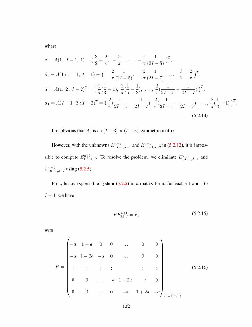
where

β = A(1 : I − 1, 1) =( 3

2+

2

π, − 2

π, . . . , − 2

π

1

(2I − 5)

)T,

β1 = A(1 : I − 1, I − 1) =(− 2

π

1

(2I − 5), − 2

π

1

(2I − 7), . . . ,

3

2+

2

π

)T,

α = A(1, 2 : I − 2)T =( 2

π(1

3− 1),

2

π(1

5− 1

3), . . . ,

2

π(

1

2I − 5− 1

2I − 7))T,

α1 = A(I − 1, 2 : I − 2)T =( 2

π(

1

2I − 5− 1

2I − 7),

2

π(

1

2I − 7− 1

2I − 9), . . . ,

2

π(1

3− 1)

)T.

(5.2.14)

It is obvious that A0 is an (I − 3)× (I − 3) symmetric matrix.

However, with the unknowns En+11:I−1,J−1 and En+1

1:I−1,J−2 in (5.2.12), it is impos-

sible to compute En+11:I−1,J . To resolve the problem, we eliminate En+1

1:I−1,J−1 and

En+11:I−1,J−2 using (5.2.5).

First, let us express the system (5.2.5) in a matrix form, for each i from 1 to

I − 1, we have

PEn+1i,1:J = F, (5.2.15)

with

P =

−a 1 + a 0 0 . . . 0 0

−a 1 + 2a −a 0 . . . 0 0

......

......

......

0 0 . . . −a 1 + 2a −a 0

0 0 . . . 0 −a 1 + 2a −a

(J−1)×(J)

(5.2.16)

122

where a = ∆t2µσh2 , F represents the RHS of this linear system.

Now, a downward recursion algorithm could be applied to the tridiagonal sys-

tem (5.2.15) eliminating the lower diagonal and yielding the diagonal element to be

unity (upper triangularization). The last two equations in the system are given by

En+1i,J−1 = pn+1

i,1 En+1i,J + qn+1

i,1 ,

En+1i,J−2 = pn+1

i,2 En+1i,J−1 + qn+1

i,2 .

(5.2.17)

Substituting the first equation of (5.2.17) into the second one, we obtain

En+1i,J−2 = pn+1

i,1 pn+1i,2 En+1

i,J + pn+1i,2 qn+1

i,1 + qn+1i,2 . (5.2.18)

Using(5.2.17) and (5.2.18), we could replaceEn+11:I−1,J−1 andEn+1

1:I−1,J−2 in (5.2.12)

to complete the linear system with respect to En+11:I−1,J and solve it by a linear solver.

With the values of En+11:I−1,J , the second step of the ADI-FDTD scheme can be im-

plemented.

Remark 1. The proposed ADI-FDTD scheme is easy and efficient to implement.

For the integral boundary condition (5.1.2), there is only one extra linear system to

compute in each iteration besides a sequence of tridiagonal linear systems. How-

ever, the extra cost is negligible since there are many fast solvers. In addition, in

each substep, the original 2D problem is transformed to a series of 1D problems

with tridiagonal linear systems.

123

5.3 Stability analysis of ADI-FDTD in L2 norm

Now, we analyze the stability of the proposed ADI-FDTD scheme for the model

(5.1.1)-(5.1.4) 1 . Firstly, define the following discrete L2 norms and the corre-

sponding inner product:

||En||2 =J−1∑

j=1

I−1∑

i=1

En2

i,jh2, ||δxEn||2 =

J−1∑

j=1

I−1∑

i=0

(δxEni+ 1

2,j)2h2,

||δzEn||2 =J−1∑

j=0

I−1∑

i=1

(δzEni,j+ 1

2

)2h2, ||δxδzEn||2 =J−1∑

j=0

I−1∑

i=0

(δxδzEni+ 1

2,j+ 1

2

)2h2,

(U, V ) =J−1∑

j=1

I−1∑

i=1

Ui,jVi,jh2,

(5.3.1)

and

||En||2Γ1=

I−1∑

i=1

En2

i,J

h2

2, ||En||2Γ2

=J−1∑

j=1

En2

I,j

h2

2,

||En||2Γ3=

I−1∑

i=1

En2

i,0

h2

2, ||En||2Γ4

=J−1∑

j=1

En2

0,j

h2

2,

(5.3.2)

where Γ1 refers to the earth-air interface, Γ2, Γ3 and Γ4 are the three subsurfaces

counterclockwise as shown in Figure 5.1.

The discrete L2 norm of E in the inner domain without boundaries is defined

by (5.3.1), and (5.3.2) gives the discrete L2 norm of E on the four boundaries

respectively. By estimating the discrete energy of this system, we will analyze the

stability of the ADI-FDTD algorithm.

1The main work in theoretical analysis of stability is conducted by Dr. Wanshan Li

124

Eliminating the intermediate variablesEn+ 1

2 from the schemes (5.2.2) and (5.2.5),

it is not hard to verify that the ADI scheme is equivalent to the following scheme

for all the inner points:

En+1i,j − En

i,j

∆t− 1

2µσ(δ2x + δ2z)(E

n + En+1)i,j +∆t

4µ2σ2δ2xδ

2z(E

n+1 − En)i,j = 0,

i = 1, . . . , I − 1, j = 1, . . . , J − 1.

(5.3.3)

Multiplying (En+En+1)i,j to both sides of (5.3.3), computing the inner product

and denoting the three items on the left hand side as I1, I2 and I3, respectively, it

follows that with the definition in (5.3.1),

I1 =

(En+1 − En

∆t, (En + En+1)

)=

1

∆t

(||En+1||2 − ||En||2

),

I2 = − 1

2µσ

((δ2x + δ2z)(E

n + En+1), (En + En+1)

),

I3 =∆t

4µ2σ2

(δ2xδ

2z(E

n+1 − En), (En + En+1)

).

(5.3.4)

Using the discrete Green formula and imposing the Neumann boundary con-

ditions on the subsurface Γ2, Γ3 and Γ4 (5.2.6), for the δ2x and δ2z terms in I2, we

deduce respectively, that

I21 = − 1

2µσ

(δ2x(E

n + En+1), (En + En+1)

)=

1

2µσ||δx(En + En+1)||2,

(5.3.5)

125

I22 = − 1

2µσ

(δ2z(E

n + En+1), (En + En+1)

)

=1

2µσ

||δz(En + En+1)||2 −

I−1∑

i=1

[(En + En+1)i,J − (En + En+1)i,J−1

]

× (En + En+1)i,J

.

(5.3.6)

In fact, the boundary schemes on subsurfaces Γ2−Γ4 (5.2.6) imply the following

relationship:

δzEn0,j+ 1

2

= δzEn1,j+ 1

2

, δzEnI,j+ 1

2

= δzEnI−1,j+ 1

2

, j = 0, · · · , J − 1,

δxEni+ 1

2,0= δxE

ni+ 1

2,1, i = 0, · · · , I − 1.

(5.3.7)

By the discrete Green formula and (5.3.7), for I3, we derive

I3 =∆t

4µ2σ2

J−1∑

j=1

I−1∑

i=1

δ2xδ2z(E

n+1 − En)i,j(En+1 + En)i,jh

2

=∆t

4µ2σ2

||δxδzEn+1||2 − ||δxδzEn||2

−I−1∑

i=0

[δx(E

n+1 − En)i+ 1

2,J − δx(E

n+1 − En)i+ 1

2,J−1

]× δx(E

n + En+1)i+ 1

2,J

.

(5.3.8)

The last terms in the RHS of (5.3.6) and (5.3.8) need to be dealt with carefully,

since they involve the values of E at the earth-air interface.

Firstly, we introduce the following lemma.

Lemma 1. Assume that E(x, z, t) is the exact solution of the IBV problem (5.1.1)-

(5.1.4), which is of sufficient smoothness, and Eni,j is the numerical solution of the

ADI-FDTD scheme (5.2.2)-(5.2.6). Then there exists a constant C independent of

126

∆t and h, such that

||En||2Γ1≤ C

I−1∑

i=1

(En2

i,J−1 + En2

i,J−2

)h2. (5.3.9)

Proof. Taking the inner product of E1:I−1,J with both sides of (5.2.12) at the n-th

time level, and considering the left-hand side EnT

1:I−1,JAEn1:I−1,J (A is of the form

(5.2.13)), we have

EnT

1:I−1,JAEn1:I−1,J

= EnT

2:I−2,JA0En2:I−2,J + EnT

1:I−1,JβEn1,J + EnT

1:I−1,Jβ1EnI−1,J

+I−2∑

k=2

En1,Jα(k − 1)En

k,J +I−2∑

k=2

EnI−1,Jα1(k − 1)En

k,J

= EnT

2:I−2,JA0En2:I−2,J + β(1)

(En2

I−1,J + En2

1,J

)+ 2β(I − 1)En

1,JEnI−1,J

+I−2∑

k=2

(α(I − k − 1) + β(I − k)

)En

k,JEnI−1,J

+I−2∑

k=2

(α(k − 1) + β(k)

)En

k,JEn1,J .

(5.3.10)

Note that A0 is a symmetric and strictly diagonal-dominant matrix, thus A0 is

positive-definite and we can estimate its eigenvalues, that is,

(3

2+

4

π(I − 3)) ≤ λ(A0) ≤ (

3

2+

8

π). (5.3.11)

In addition, by applying the Cauchy-Schwartz inequality, monotonic decreasing

127

and convergence of some series, we conclude that the bound of ||En||2Γ1is given by:

||En||2Γ1=

I−1∑

k=1

En2

k,J

h2

2≤M1

I−1∑

k=1

En2

k,J−1

h2

2+M2

I−1∑

k=1

En2

k,J−2

h2

2,

where

M1 = 1/(3C1

2− C2

1 −C1C2

4+

4C1

π(I − 3)− 50C0C1

9π

),

M2 = 1/(6C2 − 4C1C2 − C2

2 +16C2

π(I − 3)− 200C0C2

9π

),

C1, C2 are some positive constants independent of ∆t and h.

(5.3.12)

Therefore, it confirms (5.3.9) with C = maxM1

2, M2

2.

Remark 2. Lemma 1 reflects that the energy on the boundaries could be bounded

by the inner energy, that is,

||En||2Γ1≤ C||En||2. (5.3.13)

Using Lemma 1, we can treat the last terms in the RHS of I22 and I3 to present

the following result,

||En+1||2 + ∆t2

4µ2σ2||δxδzEn+1||2

≤ ||En||2 + ∆t2

4µ2σ2||δxδzEn||2 +

( ∆tM

2µσh2+

∆t2M

µ2σ2h4)(||En||2 + ||En+1||2

),

(5.3.14)

where M = max(3M1 + 1, 3M2).

128

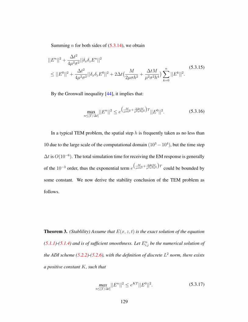
Summing n for both sides of (5.3.14), we obtain

||En||2 + ∆t2

4µ2σ2||δxδzEn||2

≤ ||E0||2 + ∆t2

4µ2σ2||δxδzE0||2 + 2∆t

( M

2µσh2+

∆tM

µ2σ2h4) n∑

k=0

||Ek||2.(5.3.15)

By the Gronwall inequality [44], it implies that:

maxn≤[T/∆t]

||En||2 ≤ e

(M

µσh2+ 2∆tM

µ2σ2h4

)T ||E0||2. (5.3.16)

In a typical TEM problem, the spatial step h is frequently taken as no less than

10 due to the large scale of the computational domain (103− 104), but the time step

∆t isO(10−6). The total simulation time for receiving the EM response is generally

of the 10−3 order, thus the exponential term e

(M

µσh2+ 2∆tM

µ2σ2h4

)T

could be bounded by

some constant. We now derive the stability conclusion of the TEM problem as

follows.

Theorem 3. (Stablility) Assume that E(x, z, t) is the exact solution of the equation

(5.1.1)-(5.1.4) and is of sufficient smoothness. Let Eni,j be the numerical solution of

the ADI scheme (5.2.2)-(5.2.6), with the definition of discrete L2 norm, there exists

a positive constant K, such that

maxn≤[T/∆t]

||En||2 ≤ eKT ||E0||2. (5.3.17)

129

5.4 Convergence analysis of ADI-FDTD

We now analyze the convergence of the proposed algorithm by the energy method.1

First, let the error define by,

ξni,j = E(xi, zj, tn)− En

i,j, i = 0, . . . , I, j = 0, . . . , J. (5.4.1)

For the truncation error at all interior and boundary grids, we have the following

Lemma.

Lemma 2. Assume that E(x, z, t) is the exact solution of the IBV problem (5.1.1)-

(5.1.4) and is of sufficient smoothness. Let Eni,j be the numerical solution of the

ADI-FDTD scheme (5.2.2)-(5.2.6), it holds that

maxi=1,...,I−1,j=1,...,J−1

|Rn+ 1

2

i,j |≤ O(∆t2 + h2),

maxj=0,...,J

|ξn0,j|, |ξnI,j|

≤ O(∆t2 + h2),

maxi=1,...,I−1

|ξni,0|, |Rn

i,J |≤ O(∆t2 + h2),

(5.4.2)

where Rn+ 1

2

i,j denotes the truncation error for the interior points, ξnI,j , ξni,0, ξ

n0,j rep-

resent the truncation errors on the three subsurfaces Γ2 −Γ4, respectively and Rni,J

is the truncation error at the earth-air interface Γ1.

Proof. For the interior points, from the inner equivalent scheme (5.3.3), we derive

1The main work in theoretical analysis of convergence is conducted by Dr. Wanshan Li

130

the error equation:

ξn+1i,j − ξni,j

∆t− 1

2µσ(δ2x + δ2z)(ξ

n + ξn+1)i,j+∆t

4µ2σ2δ2xδ

2z(ξ

n+1 − ξn)i,j = Rn+ 1

2

i,j ,

i = 1, . . . , I − 1, j = 1, . . . , J − 1.

(5.4.3)

By Taylor expansion,

Rn+ 1

2

i,j =E(xi, zj, t

n+1)− E(xi, zj, tn)

∆t− 1

2µσ(δ2x + δ2z)

E(xi, zj, t

n)

+ E(xi, zj, tn+1)

+

∆t

4µ2σ2δ2xδ

2z

E(xi, zj, t

n+1)− E(xi, zj, tn)

= O(∆t2 + h2), i = 1, . . . , I − 1, j = 1, . . . , J − 1.

(5.4.4)

Secondly, in view of the boundary schemes for the subsurfaces (5.2.6), by Tay-

lor expansion, we have,

ξn0,j = E(x0, zj, tn)− En

0,j = ξn1,j −h2

2

∂2E

∂x2(x0, zj, t

n) +O(h3), j = 0, . . . , J.

(5.4.5)

Similarly,

ξnI,j = ξnI−1,j −h2

2

∂2E

∂x2(xI , zj, t

n) +O(h3), j = 0, . . . , J,

ξni,0 = ξni,1 −h2

2

∂2E

∂z2(xi, z0, t

n) +O(h3), i = 0, . . . , I.

(5.4.6)

By considering the scheme for the earth-air interface (5.2.9) and (5.2.10), we

131

have the corresponding error equation

3ξni,J − 4ξni,J−1 + ξni,J−2

2h+

1

π

I−2∑

k=1

ξnk+1,J − ξnk,Jxi − xk+ 1

2

= Rni,J , i = 1, . . . , I − 1.

(5.4.7)

Using Taylor expansion and the upward continuation (5.1.2), we have:

Rni,J =

3E(xi, zJ , tn)− 4E(xi, zJ−1, t

n) + E(xi, zJ−2, tn)

2h

+1

π

I−2∑

k=1

E(xk+1, zJ , tn)− E(xk, zJ , t

n)

xi − xk+ 1

2

= O(h2). (since the mid-point integral formula is O(h2))

(5.4.8)

To derive the error estimation for the ADI-FDTD scheme in the discrete L2

norm, multiplying both sides of (5.4.3) with (ξni,j + ξn+1i,j ) and computing the inner

product, we obtain

Err1 =

(ξn+1 − ξn

∆t, ξn+1 + ξn

)=

1

∆t

(||ξn+1||2 − ||ξn||2

),

Err2 =

(− 1

2µσ

(δ2x + δ2z

)(ξn + ξn+1

), ξn + ξn+1

)= Err21 + Err22 ,

Err3 =

(∆t

4µ2σ2δ2xδ

2z

(ξn+1 − ξn

), ξn+1 + ξn

),

Err4 =

(Rn+ 1

2 , ξn + ξn+1

).

(5.4.9)

Since Err21 , Err22 , Err3 and Err4 are estimated using Lemma 2 and similar

method as that for the stability analysis, thus we will omit the detailed procedures

132

and present the final conclusion,

||ξn||2 + ∆t2

4µ2σ2h2||δxδzξn||2 ≤ ||ξ0||2 + ∆t2

4µ2σ2h2||δxδzξ0||2

+∆t(1 +

M0

µσh2+

2∆tM0

µ2σ2h4) n∑

k=1

||ξk||2 +O(∆t4 + h4).

(5.4.10)

Notice that ξ0i,j = 0, and by the Gronwall Lemma, we obtain the following

theorem.

Theorem 4. (Convergence) Assume that E(x, z, t) is the exact solution of the IVB

problem (5.1.2)-(5.1.4) and is of sufficient smoothness, let Eni,j be the numerical so-

lution of the ADI-FDTD scheme (5.2.2)-(5.2.6) and define error ξni,j = E(xi, zj, tn)−

Eni,j , then there exists a positive constant M , such that

maxn≤[T/∆t]

||ξn||2 ≤M(∆t2 + h2). (5.4.11)

5.5 Numerical Simulations

To validate the proposed ADI-FDTD scheme for 2D TEM models, we present the

computational results for the following test cases. Particular attentions will focus on

demonstrating the accuracy and performance advantages of the presented algorithm

over the popular FDTD method based on DuFort-Frankel method. Three test cases

have been taken as test examples to validate our ADI-FDTD considered in [76].

133

5.5.1 Half-space

As a first check of the proposed numerical algorithm, we compute the responses of

a homogeneous half-space to the shut-off of a steady current in a double line source

at the surface. The test case is chosen because the analytical solution is available

for both the electric field at the surface and in the half-space. The initial condition

is taken as that reported in [76].

The computational domain is [0,32000m]×[0,10000m] and the double line source

is set at the centre of the earth-air interface with the negative limb located at x =16250m

and the positive limb at x =15750m. The current is I =1A and the electric con-

ductivity of the ground is σ =1/300S/m.

In our simulations, the inhomogeneous grids are adopted along x and z direc-

tions with an increasing step size according to the distance from the source, with the

smallest step size ∆x = ∆z = hmin =10m for the grids near the source. In terms

of the initial condition, we take t0 = 2.0×10−6 and the top eight-layer electric field

is assigned. The time step ∆t used in the computation is listed in Table 5.1.

Table 5.1: Time steps in second for the ADI-FDTD and DF schemes

response time(ms) ∆t for DF ∆t for ADI-FDTD

(0, 0.1) 1.1793e-7 9.4345e-7

(0.1, 1) 1.1793e-6 1.8869e-5

> 1 2.3586e-6 3.7738e-5

134

1.2 1.3 1.4 1.5 1.6 1.7 1.8 1.9 2

x 104

−1.5

−1

−0.5

0

0.5

1

1.5x 10

−4

x (m)

Ver

tica

l E

MF

(V

/m2) Exact solution

ADI−FDTD scheme

DF scheme

(a) T = 0.007ms

1.2 1.3 1.4 1.5 1.6 1.7 1.8 1.9 2

x 104

−1

0

1

2

3

4x 10

−6

x (m)

Ver

tica

l E

MF

(V

/m2) Exact solution

ADI−FDTD scheme

DF scheme

(b) T = 0.1ms

1.2 1.3 1.4 1.5 1.6 1.7 1.8 1.9 2

x 104

−5

0

5

10

15x 10

−9

x (m)

Ver

tica

l E

MF

(V

/m2) Exact solution

ADI−FDTD scheme

DF scheme

(c) T = 3ms

1.2 1.3 1.4 1.5 1.6 1.7 1.8 1.9 2

x 104

−1

0

1

2

3x 10

−10

x (m)

Ver

tica

l E

MF

(V

/m2) Exact solution

ADI−FDTD scheme

DF scheme

(d) T = 15ms

Figure 5.2: Comparison of analytical and numerical solutions computed by the

ADI-FDTD and DF schemes for the vertical EMF (∂tBz) induced by a double line

source on a half-space. Profiles are at (a)0.007 ms, (b)0.1 ms, (c)3 ms, (d)15 ms

after the source current was switched off.

135

Table 5.2: CPU time in second for the ADI-FDTD and DF schemes

simulation time(ms) DF ADI-FDTD

0.007 9 52

0.1 128 265

3 442 482

15 1292 1240

0 5 10 1510

−3

10−2

10−1

100

Response Time (ms)

Rel

ativ

e E

rrors

( l

og

10 )

ReError1 of ADI−FDTD

ReError1 of DF

ReError2 of ADI−FDTD

ReError2 of DF

Figure 5.3: Relative L∞ and L2 errors for the ADI-FDTD and DF schemes

−4e−006

−2e−006

0

0

02e−006

4e−006

6e−006

(a) T = 3ms

−1e−006

−8e−007−

6e−007

−6e−007

−4e−007

−4e−007

−2e−007

−2e−007

0

0

0

2e−007

2e−007

2e−007

4e−007

4e−007

6e−007

6e−007

8e−007

1e−006

(b) T = 10ms

−5e−007

−4e−007

−4e−007

−3e−007

−3e−007

−2e−007

−2e−007

−2e−007

−1e−007

−1e−007

−1e−007

0

0

0

1e−007

1e−007

1e−007

2e−007

2e−007

2e−007

3e−007

3e−007

4e−007

4e−007

5e−007

(c) T = 15ms

−3e−007

−3e−007

−2e−007

−2e−007

−1e−007

−1e−007

−1e−007

0

0

0

1e−007

1e−007

1e−007

2e−007

2e−007

3e−007

3e−007

(d) T = 21ms

Figure 5.4: Contours of electric field in a half-space computed by the ADI-FDTD

scheme induced by a switched-off 500m wide double line source at the earth-air

interface. Profiles are at (a)3 ms, (b)10 ms, (c)15 ms, (d)21 ms after source current

was switched off.136

We now compare the performance of the developed ADI-FDTD scheme and that

based on DF method [76]. The DF scheme is also unconditionally stable, but the

time step ∆t could not be taken very large in numerical simulations since oscillatory

solutions might occur. Compared with the DF-FDTD method, it is worth to note

that more accurate numerical results could be achieved by using the proposed ADI-

FDTD algorithm.

Using the time steps listed in Table 5.1, the solution snapshots are shown in

Figure 5.2, and the corresponding CPU times are reported in Table 5.2. Due to the

transient of the initial electric fields, at the very beginning (generally before 0.1ms),

the time steps must be chosen small enough to describe the responses without dis-

tortion. Thus it gives rise to a little longer CPU times for the ADI-FDTD method

than the DF scheme at the early time. However, consider that the early time is

very short compared with the total computational time, the improvement in accu-

racy (Ref. Figure 5.2, Figure 5.3) is more significant. In practical applications, the

late time responses are generally required instead of the early time responses. From

Table 5.2, after 3ms, the CPU times for these two algorithms are of the same order.

The vertical electromotive force (EMF) at the earth-air interface of the numer-

ical solution and the exact solution are shown in Figure 5.2, and they could be

obtained by measurement. Figure 5.2(a) and Figure 5.2(b) present the short time

response to the switched-off of the current in the double line source, while Figure

5.2(c) and Figure 5.2(d) are the long time responses. The relative L∞ and L2 er-

137

rors defined as follows are also illustrated in Figure 5.3 with respect to the response

time. It is obvious to see that the ADI-FDTD scheme with large time steps produces

more accurate solutions than the DF scheme with relatively small time steps. The

advantage of using the presented method is clear especially for computing the late

time solution. Figure 5.3 confirms that when comparing with the numerical solu-

tions by the DF scheme, an improvement in accuracy of an order of magnitude can

be achieved by using the ADI-FDTD scheme.

ReError1 =||Enumerical − Eexact||L∞(Γ1)

||Eexact||L∞(Γ1)

,

ReError2 =||Enumerical − Eexact||L2(Γ1)

||Eexact||L2(Γ1)

.

Figure 5.4 gives the contours of the electric field in the whole simulation do-

main, which illustrates the profile of the induced field propagation. We clearly ob-

serve the diffusion of the smoke ring profiles for the electric field as time marching

forward.

5.5.2 Half-space with conductor (large contrast)

The second test case shown in Figure 5.5 is to model a 300Ω-m half-space con-

taining a thin rectangular ore body with the electric conductivity 1000 times more

than the surroundings. The thin ore body with the scale of 20m×300m located at

300m away from the negative line source to the left along the x direction, thus the

distance of the ore body from the center of double line source is about 550m.

In this example, the time steps for the simulation are taken as in Table 5.3. For

138

the sake of exhibiting the influence of the anomaly elaborately, a small enough ∆t

is set for the very early time till 0.01ms. Furthermore, to demonstrate the efficiency

and effectiveness of the proposed scheme, we adopt a larger time steps after 0.01ms,

compared with DF scheme, as shown in Table 5.3. The vertical EMF, horizontal

EMF curves and contours of the electric field induced by the switched-off of double

line source are reported in Figure 5.6, Figure 5.7 and Figure 5.8, respectively.

300m

300m

100m500m

σh=0.0033 S/m

σb=3.33 S/m

+ −

20m

Figure 5.5: Model geometry for half-space with large-contrast conductor.

The vertical EMF (−∂tBz) profiles using the ADI-FDTD algorithm in Figure

5.6 are featured by the crossover from positive to negative values on account of

the existence of the thin vertical conductor, and the location of crossover in Figure

5.6 is gradually moving to the exact horizontal position of the thin anomaly. In

addition, the peak of the horizontal EMF (−∂tBx) using the ADI-FDTD algorithm

displayed in Figure 5.7 could also serve to examine the horizontal position of the

thin body approximately.

139

Figure 5.6: Profiles of the vertical EMF (∂tBz) by the ADI-FDTD scheme for the

half-space conductor with a 1000:1 contrast. The negative line source is on the

right. Open marks indicate negative values and dark marks represent positive ones.

Figure 5.7: Profiles of the horizontal EMF (∂tBx) by the ADI-FDTD scheme for

the half-space conductor with a 1000:1 contrast. The negative line source is on the

right. Open marks indicate negative values.

Table 5.3: Time steps in second for ADI-FDTD and DF schemes

response time(ms) ∆t for DF ∆t for ADI-FDTD

(0, 0.01) 4.7172e-8 4.7172e-8

(0.01, 0.1) 1.1793e-7 9.4345e-7

(0.1, 1) 1.1793e-6 1.8869e-5

> 1 2.3586e-6 3.7738e-5

140

−45

−40

−35−

35

−30

−30

−30

−25

−25

−25 −25−25

−20

−20

−20 −20−20

−20−1

5

−15

−15

−15

−15

−15

−10

−10

−10 −10

−10

−10−5

−5

−5

−5

−5

−5

20 40 60 80 100

10

20

30

40

50

60

(a) ADI, T = 0.006ms

−45

−40 −

35

−35

−30

−30

−30 −30 −30

−25

−25

−25 −25 −25

−20

−20

−20 −20−20

−20−15

−15

−15

−15

−15

−15

−10

−10

−10

−10 −10−10

−5

−5

−5

−5

−5

−5

20 40 60 80 100

10

20

30

40

50

60

(b) DF, T = 0.006ms

−22

−20

−18−

18

−16

−16 −

14

−14

−14 −14−12

−12

−12

−12 −12

−12

−12

−10

−10

−10

−10

−10

−10

−10−8

−8

−8

−8

−8

−8−

8−8

−6

−6

−6

−6

−6

−6

−6

−4

−4

−4

−4

−4

−4

20 40 60 80 100

10

20

30

40

50

60

(c) ADI, T = 0.015ms

−25

−20−2

0 −15

−15

−15 −15

−10

−10

−10

−10

−10

−10

−10

−5

−5

−5

−5

−5

−5

−5

20 40 60 80 100

10

20

30

40

50

60

(d) DF, T = 0.015ms

−13

−12

−11−

11

−10

−10

−9

−9

−9

−9

−9

−8

−8

−8 −8

−8

−7

−7

−7

−7

−7

−7

−7

−7−

7

−6

−6

−6

−6

−6

−6

−6

−6

−6

−5

−5

−5

−5

−5

−5

−5

−5

−5

−4

−4

−4

−4

−4

−4 −4

−3

−3

−3

−3

−3

20 40 60 80 100

10

20

30

40

50

60

(e) ADI, T = 0.036ms

−13

−12 −

11

−11

−10

−10

−9

−9

−9

−9

−9

−8

−8−8

−8

−8

−7

−7

−7

−7

−7

−7

−7

−7−

7

−6

−6

−6

−6

−6

−6

−6

−6

−6

−5

−5

−5

−5

−5

−5

−5

−5

−5

−4

−4

−4

−4

−4

−4

−4

−3

−3

−3

−3

−3

20 40 60 80 100

10

20

30

40

50

60

(f) DF, T = 0.036ms

141

142

143

−6.8

−6.6 −6.4

−6.4

−6.2

−6.2

−6.2

−6

−6

−6

−5.8

−5.8

−5.8

−5.6

−5.6

−5.6

−5.6

−5.6

−5.4

−5.4

−5.4

20 40 60 80 100

10

20

30

40

50

60

(g) ADI, T = 9ms−6.8

−6.6

−6.4

−6.2

−6.2

−6.2

−6

−6

−6

−5.8

−5.8

−5.8

−5.6

−5.6

−5.6

−5.6

−5.4

−5.4

−5.4 −

5.4

20 40 60 80 100

10

20

30

40

50

60

(h) DF, T = 9ms

−6.1

−6.1

−6

−6

−6

−5.9

−5.9

−5.9

−5.8

−5.8

−5.8 −

5.8

−5.7

−5.7

−5.7

−5.7

−5.7

−5.6

−5.6

−5.6

−5.5

20 40 60 80 100

10

20

30

40

50

60

(i) ADI, T = 15ms

−6.1

−6

−6

−6

−5.9

−5.9

−5.9

−5.8

−5.8

−5.8

−5.7

−5.7

−5.7

−5.7

−5.7

−5.6

−5.6

−5.6

−5.6

−5.5

−5.5

20 40 60 80 100

10

20

30

40

50

60

(j) DF, T = 15ms

−6.15

−6.1

−6.1

−6.1

−6.05

−6.05

−6.05

−6

−6

−6

−5.95

−5.95

−5.95

−5.9

−5.9

−5.9 −

5.9

−5.85

−5.85

−5.85 −

5.85

−5.85

−5.8

−5.8

−5.8

−5.8

−5.8

−5.75

−5.75

−5.75

−5.75

−5.7

−5.7

−5.7

−5.65

−5.65

20 40 60 80 100

10

20

30

40

50

60

(k) ADI, T = 20ms

−6.1

−6.05

−6.05

−6.05

−6

−6

−6

−5.95

−5.95

−5.95

−5.9

−5.9

−5.9

−5.85

−5.85

−5.85 −

5.85

−5.8

−5.8

−5.8 −

5.8

−5.8

−5.75

−5.75

−5.75

−5.75

−5.75

−5.7

−5.7

−5.7

−5.7

−5.65−

5.65

−5.65

−5.6

−5.6

20 40 60 80 100

10

20

30

40

50

60

(l) DF, T = 20ms

Figure 5.8: Contours of electric field(the values are the logarithm of E) computed

by the ADI-FDTD scheme(on the left) and the DF scheme(on the right) for the half-

space with the conductor of 1000:1, induced by a switched-off 500m wide double

line source at the earth-air interface.

144

Figure 5.8 compares the contours of the electric fields for this large contrast

model using ADI-FDTD scheme(on the left) as well as the DF scheme(on the right)

and the snapshots presented cover a wide range of time from the very early time

0.006ms to the late time 20ms. It is clear to observe that the two sets of results

are generally consistent with each other except for some subtle distinction. Results

by the ADI-FDTD method capture the responses well for both early times and late

times.

To illustrate the characters of the electric field around the thin conductor and

double line source, only the central and uniform regions of the numerical grids

are shown. The crossover on the left of the first four subfigures makes clear the

position of the source center, while the crossover on the right highlights the main

domain containing the thin conductor. The following subfigures reflect that when

the diffusion of electric field encounters the thin anomaly, they are distorted by

the interaction with this conductor. The snapshot taken at 3.7ms displays a fully

developed target response and the further evolution of the electric field involves its

gradual equalization and decay within the conductor.

5.5.3 Half-space with conductor (small contrast)

We now consider a small contrast(100:1) version of the second test model as illus-

trated in Figure 5.9 1. The parameters for this simulation are set the same as those

1The figures in this section and following sections are prepared by Dr. Wanshan Li

145

in the large contrast case, except that the half-space resistivity is 100Ω-m, while the

body resistivity is 1Ω-m.

From the vertical EMF presented in Figure 5.10, it is clear that even though

the crossover appears at nearly the exact target position at 1 ms, it moves to the

right and away from the target with time advancing. This may be attributed to the

currents in the half-space, whose contribution covers some of the effect from the

currents flowing in the ore body.

On the other hand, the horizontal EMF profiles shown in Figure 5.11 obvious-

ly illustrate the location of the anomaly by their peaks. Generally, in contrast to

the crossover point of the vertical EMF, the peak in the horizontal EMF is always

directly above the target in the millisecond time range and thus giving a better in-

dication of the conductor location. We also report the snapshots by the ADI-FDTD

and DF schemes in Figure 5.12 to reveal some details of the development of the

electric field in early time and later the interaction between the smoke ring and the

conductor, and their results are in good agreement.

300m

300m

100m500m

σh=0.01 S/m

σb=1.0 S/m

+ −

20m

Figure 5.9: Model geometry for overburden and half-space with small-contrast con-

ductor.

146

Figure 5.10: Profiles of the vertical EMF (∂tBz) by the ADI-FDTD scheme for the

half-space with small contrast conductor model. The negative line source is on the

right. Open marks indicate negative values and dark marks represent positive ones.

Figure 5.11: Profiles of the horizontal EMF (∂tBx) by the ADI-FDTD scheme for

the half-space with small contrast conductor model. The negative line source is on

the right. Open marks indicate negative values.

147

−16

−14

−12

−12

−10

−10

−10 −10−8

−8

−8

−8

−8

−8

−8

−8

−6

−6

−6

−6

−6 −6

−6

−6

−4

−4

−4

−4

−4

−4

20 40 60 80 100

10

20

30

40

50

60

(a) ADI, T = 0.08ms

−16

−14

−12

−12

−10

−10

−10 −10−8

−8

−8

−8

−8

−8

−8

−8

−6

−6

−6

−6

−6 −6

−6

−6

−4

−4

−4

−4

−4

−4

20 40 60 80 100

10

20

30

40

50

60

(b) DF, T = 0.08ms

−6

−6

−5.5

−5.5

−5.5−

5.5

−5.5

−5.5 −5

.5−5

−5

−5

−5

−5

−5

−5

−5

−5

−4.5

−4.5

−4.5

−4.5

−4.5 −

4.5

−4.5

−4.5

−4

−4

−4

−4

20 40 60 80 100

10

20

30

40

50

60

(c) ADI, T = 0.5ms

−6

−6

−5.5

−5.5

−5.5−

5.5

−5.5

−5.5

−5.5

−5

−5

−5

−5

−5

−5 −

5

−5

−5

−4.5

−4.5

−4.5

−4.5

−4.5

−4.5

−4.5

−4.5

−4

−4

−4

−4

−4

20 40 60 80 100

10

20

30

40

50

60

(d) DF, T = 0.5ms

−7

−7

−6.5

−6.5

−6.5

−6.5

−6

−6

−6

−6

−6

−6

−5.5

−5.5

−5.5

−5.5

−5.5

−5.5

−5

−5

−5

−5

−5

−5

−5

−4.5

−4.5

−4.5

−4.5

20 40 60 80 100

10

20

30

40

50

60

(e) ADI, T = 1ms

−7

−7

−6.5

−6.5

−6

−6

−6

−6

−6

−6

−5.5

−5.5

−5.5

−5.5

−5.5

−5.5

−5

−5

−5

−5

−5

−5

−5

−4.5

−4.5

−4.5

−4.5

−4.5

−4.5

20 40 60 80 100

10

20

30

40

50

60

(f) DF, T = 1ms

−7

−7

−7

−7

−6.5

−6.5

−6.5

−6.5

−6.5

−6.5

−6

−6

−6

−6

−6

−6

−5.5

−5.5

−5.5

−5.5

−5.5

−5.5

−5

−5

−5

−5

−5

−5

−5

20 40 60 80 100

10

20

30

40

50

60

(g) ADI, T = 1.6ms

−8

−8

−7

−7−7

−7

−7

−6

−6

−6

−6

−6

−6

−5

−5

−5

−5

−5

−5 −

5

20 40 60 80 100

10

20

30

40

50

60

(h) DF, T = 1.6ms

148

−7.5

−7.5

−7

−7

−7

−7

−7

−7

−6.5

−6.5

−6.5

−6.5

−6.5

−6.5

−6

−6

−6

−6

−6

−6

−5.5

−5.5

−5.5

−5

20 40 60 80 100

10

20

30

40

50

60

(i) ADI, T = 5ms

−7

−7

−7

−7

−7

−7

−6.5

−6.5

−6.5

−6.5

−6.5

−6.5

−6

−6

−6

−6

−6

−6

−5.5

−5.5

−5.5

−5.5

−5.5

−5

−5

−5

20 40 60 80 100

10

20

30

40

50

60

(j) DF, T = 5ms

−8

−8

−8

−8

−8

−8

−8

−8

−8

−8

−8

−8

−8

−7.5

−7.5

−7.5

−7.5

−7.5−7

−7

−7

−7

−7

−6.5

−6.5

−6.5

−6.5

−6

−6

−6

−5.5−

5.5

−5.5

−5.5

−5.5

20 40 60 80 100

10

20

30

40

50

60

(k) ADI, T = 9ms

−8

−8

−8

−8

−8

−8

−8

−8

−8

−8

−8

−7.5

−7.5

−7.5

−7.5

−7.5−7

−7

−7

−7

−7

−6.5

−6.5

−6.5

−6.5

−6

−6

−6

−5.5

−5.5

−5.5

20 40 60 80 100

10

20

30

40

50

60

(l) DF, T = 9ms

−6.8 −6.6

−6.6

−6.4

−6.4

−6.4

−6.2

−6.2

−6.2

−6

−6

−6

−5.8

−5.8

20 40 60 80 100

10

20

30

40

50

60

(m) ADI, T = 15ms

−6.8

−6.6

−6.4

−6.4

−6.4

−6.2

−6.2

−6.2

−6

−6

−6

−5.8

−5.8

−5.8

20 40 60 80 100

10

20

30

40

50

60

(n) DF, T = 15ms

−6.8

−6.7

−6.7

−6.7

−6.6

−6.6

−6.6

−6.5

−6.5

−6.5

−6.4

−6.4

−6.4

−6.3

−6.3

−6.3

−6.2

−6.2

−6.2

−6.1

−6.1

−6.1 −6.1

20 40 60 80 100

10

20

30

40

50

60

(o) ADI, T = 20ms

−6.7

−6.6

−6.6

−6.6

−6.5

−6.5

−6.5

−6.4

−6.4

−6.4

−6.3

−6.3

−6.3

−6.2

−6.2

−6.2

−6.1

−6.1

−6.1

−6

−6

−6

−6

20 40 60 80 100

10

20

30

40

50

60

(p) DF, T = 20ms

Figure 5.12: Contours of electric field(the values are the logarithm of E) computed

by the ADI-FDTD scheme(on the left) and the DF scheme(on the right) for the half-

space with small contrast conductor model, induced by a switched-off 500m wide

double line source at the earth-air interface.149

5.6 Concluding Remarks

We present an efficient and accurate ADI-FDTD algorithm to simulate EM diffu-

sion phenomenon in a 2D earth excited by the electric line sources. Comparisons

with the analytical and DuFort-Frankel solutions confirm the accuracy and efficien-

cy of the proposed algorithm. The ADI technique is applied such that the resultant

tri-diagonal system can be effectively computed by the Thomas algorithm. To en-

sure an accurate representation for the earth-air interface, an integral formulation is

imposed at the interface boundary. A novel numerical discretization scheme for the

integral equation is presented and it is incorporated to the ADI scheme implicitly.

With the numerical implementation for the integral boundary condition, the stability

and convergence analysis for the ADI-FDTD scheme are reported. Numerical sim-

ulations clearly demonstrate that the proposed ADI-FDTD scheme produces more

accurate computed solutions than those resulted by the DuFort-Frankel scheme both

in the early time and late time computation.

It is worth to investigate further applications and improvements of the proposed

ADI-FDTD algorithm. For example, consider using the secondary field instead of

total field in the model. Secondary field is defined as the difference between the

total field and the field of a background model, and they vary more slowly than

the total field in both time and space. The application of an absorbing boundary

condition including a perfectly matched layer (PML) for the underground interface

150

is also an interesting topic. Finally, it is important to extend the present approach

for 2.5D and 3D problems.

The work reported in this chapter has been accepted and will appear in Com-

munications in Computational Physics [63].

151

Chapter 6

Conclusion

This thesis is focused on the numerical analysis and mathematical modeling for the

geophysical exploration problems. Potential field inversion is an important meth-

ods related to mining and oil industry. By measuring the potential field and apply

the inversion schemes to the observation data, the underground structure can be re-

covered. The numerical inversion scheme is the key to the quality of the recovered

model. Conventional inversion schemes require a huge amount of computational

cost and storage requirement, which can be only run on super computer clusters.

In Chapter 2, we present a novel computational method based on conjugate gra-

dient method. Taking advantage of Block-Toeplitz Toeplitz-Block structure, we

develop a robust and efficient downward continuation scheme. The method is vali-

dated on synthetic and field data, and its superiority is verified by comparing with

recently developed wavenumber domain and Taylor series methods.

Chapter 3 presents an efficient numerical inversion scheme using the idea of

multi-grid technique. The scheme is efficient for the aeromagnetic field data. The

most important feature of the proposed method is that it preserves the BTTB struc-

ture in each level, such that the error with different frequencies can be efficiently

152

removed. By synthetic and field simulation, we have shown that the BTTB-MG

method is a competitive alternative to a regularized method, particularly when a

high accuracy is required for the perturbed data.

Chapter 4 presents the 3D gravity field inversion problem. Compared with the

2D inversion problem, 3D inversion is much more challenging due to the complexi-

ty of the model and extremely heavy computational work load. It is reported that for

the inversion with several million unknowns, the time cost of the inversion scheme

can be as high as hundreds of hours by using super workstation. We expand our 2D

method to the 3D gravity inversion, and made several improvements for both the

regularization and preconditioner. Numerical simulations based on synthetic and

real data show that for the 3D inversion with several million unknowns, our numer-

ical scheme can be run on a laptop within several minutes to finish the inversion

process. Besides, we give the strict mathematical proofs for the convergence and

consistency of the numerical solution, which has not been investigated before.

In chapter 5, we investigate the electromagnetic method in exploration, which is

based on modeling the electromagnetic (EM) wave diffusion underground to recov-

er the conductivity distribution. EM problem is a very challenging problem in terms

of algorithm complexity and stability. We proposed an implicit ADI-FDTD scheme

to simulate the diffusion behavior of the EM wave. The time and space grids in our

proposed scheme can be much larger than that in the conventional Du-Fort-Frankel

method, while the accuracy of the numerical solution is superior to the conventional

153

method for an order.

154

Bibliography[1] J. Abbiss and P. Earwicker. Compact operator equations, regularization and

super-resolution. Mathematics in Signal Processing, T. Durrani et al., eds.,

Clarendon Press, Oxford, 1987.

[2] J. I. Adhidjaja, G. W. Hohmann, and M. L. Oristaglio. Two-dimensional

transient electromagnetic responses. Geophysics, 50(12):2849–2861, 1985.

[3] M. B. Allen and E. L. Isaacson. Numerical analysis for applied science,

volume 35. John Wiley & Sons, 2011.

[4] U. Ascher and E. Haber. Grid refinement and scaling for distributed param-

eter estimation problems. Inverse Problems, 17(3):571, 2001.

[5] A. Asnaashari, R. Brossier, S. Garambois, F. Audebert, P. Thore, and

J. Virieux. Regularized seismic full waveform inversion with prior model

information. Geophysics, 78(2):R25–R36, 2013.

[6] H. R. Babu, A. Subrahmanyam, and D. A. Rao. A comparative study of

the relation figures of magnetic anomalies due to two-dimensional dike and

vertical step models. Geophysics, 47(6):926–931, 1982.

[7] M. Beiki and L. B. Pedersen. Eigenvector analysis of gravity gradient tensor

to locate geologic bodies. Geophysics, 75(6):I37–I49, 2010.

[8] A. Bjorck. Numerical methods for least squares problems. SIAM, 1996.

[9] R. J. Blakely. Potential theory in gravity and magnetic applications. Cam-

bridge University Press, 1996.

[10] I. C. Briggs. Machine contouring using minimum curvature. Geophysics,

39(1):39–48, 1974.

[11] W. L. Briggs and S. F. McCormick. A multigrid tutorial, volume 72. SIAM,

2000.

155

[12] A. G. Camacho, F. G. Montesinos, and R. Vieira. Gravity inversion by means

of growing bodies. Geophysics, 65(1):95–101, 2000.

[13] F. Caratori Tontini, L. Cocchi, and C. Carmisciano. Rapid 3-D forward

model of potential fields with application to the Palinuro seamount magnetic

anomaly (southern Tyrrhenian sea, Italy). Journal of Geophysical Research:

Solid Earth (1978–2012), 114(B2), 2009.

[14] R. Cassinis. The solution of the inverse problem in geophysical interpreta-

tion, volume 11. Springer Science & Business Media, 2013.

[15] R. H. Chan and X. Q. Jin. An introduction to iterative Toeplitz solvers, vol-

ume 5. SIAM, 2007.

[16] R. H. Chan, J. G. Nagy, and R. J. Plemmons. FFT-based preconditioners for

Toeplitz-Block least squares problems. SIAM journal on numerical analysis,

30(6):1740–1768, 1993.

[17] R. H. Chan and M. K. Ng. Conjugate gradient methods for Toeplitz systems.

SIAM review, 38(3):427–482, 1996.

[18] W. Chen, X. Li, and D. Liang. Symmetric energy-conserved splitting FDTD

scheme for the Maxwell’s equations. Communications in Computational

Physics, 6(4):804–825, 2009.

[19] Y. Chung, J.-S. Son, T. J. Lee, H. J. Kim, and C. Shin. Three-dimensional

modelling of controlled-source electromagnetic surveys using an edge finite-

element method with a direct solver. Geophysical Prospecting, 2014.

[20] G. K. Clarke. Optimum second-derivative and downward-continuation filter-

s. Geophysics, 34(3):424–437, 1969.

[21] M. Commer and G. Newman. A parallel finite-difference approach for

3D transient electromagnetic modeling with galvanic sources. Geophysic-

s, 69(5):1192–1202, 2004.

[22] S. Constable and C. J. Weiss. Mapping thin resistors and hydrocarbons with

marine EM methods: Insights from 1D modeling. Geophysics, 71(2):G43–

G51, 2006.

156

[23] G. Cooper. Gridding gravity data using an equivalent layer. Computers &

Geosciences, 26(2):227–233, 2000.

[24] G. Cooper. The stable downward continuation of potential field data. Explo-

ration Geophysics, 35(4):260–265, 2004.

[25] L. Cordell. A scattered equivalent-source method for interpolation and grid-

ding of potential-field data in three dimensions. Geophysics, 57(4):629–636,

1992.

[26] L. H. Cox, G. A. Wilson, and M. S. Zhdanov. 3D inversion of airborne

electromagnetic data using a moving footprint. Exploration Geophysics,

41(4):250–259, 2010.

[27] M. Cuma, G. A. Wilson, and M. S. Zhdanov. Large-scale 3D inversion of

potential field data. Geophysical Prospecting, 60(6):1186–1199, 2012.

[28] N. V. Silva, J. V. Morgan, L. MacGregor, and M. Warner. A finite element

multifrontal method for 3D csem modeling in the frequency domain. Geo-

physics, 77(2):E101–E115, 2012.

[29] K. Davis and Y. Li. Fast solution of geophysical inversion using adaptive

mesh, space-filling curves and wavelet compression. Geophysical Journal

International, 185(1):157–166, 2011.

[30] K. Davis and Y. Li. Efficient 3D inversion of magnetic data via octree-mesh

discretization, space-filling curves, and wavelets. Geophysics, 78(5):J61–

J73, 2013.

[31] P. J. Davis. Circulant matrices. American Mathematical Soc., 1979.

[32] W. C. Dean. Frequency analysis for gravity and magnetic interpretation.

Geophysics, 23(1):97–127, 1958.

[33] L. Elden. An algorithm for the regularization of ill-conditioned, banded

least squares problems. SIAM journal on scientific and statistical comput-

ing, 5(1):237–254, 1984.

157

[34] M. Everett and R. Edwards. Transient marine electromagnetics: the 2.5-

D forward problem. Geophysical Journal International, 113(3):545–561,

1993.

[35] M. Fedi and G. Florio. Detection of potential fields source boundaries by

enhanced horizontal derivative method. Geophysical prospecting, 49(1):40–

58, 2001.

[36] M. Fedi and G. Florio. A stable downward continuation by using the ISVD

method. Geophysical Journal International, 151(1):146–156, 2002.

[37] R. W. Freund and N. M. Nachtigal. An implementation of the QMR method

based on coupled two-term recurrences. SIAM Journal on Scientific Com-

puting, 15(2):313–337, 1994.

[38] L. Gao and D. Liang. New energy-conserved identities and super-

convergence of the symmetric EC-S-FDTD scheme for Maxwell’s equations

in 2D. Communications in Computational Physics, 11(5):1673–1696, 2012.

[39] A. Garcıa-Yeguas, I. Koulakov, J. M. Ibanez, and A. Rietbrock. High reso-

lution 3D p wave velocity structure beneath Tenerife island (Canary islands,

spain) based on tomographic inversion of active-source data. Journal of Geo-

physical Research: Solid Earth (1978–2012), 117(B9), 2012.

[40] S. P. Gay Jr. Standard curves for interpretation of magnetic anomalies over

long tabular bodies. Geophysics, 28(2):161–200, 1963.

[41] Y. Goldman, C. Hubans, S. Nicoletis, and S. Spitz. A finite-element solution

for the transient electromagnetic response of an arbitrary two-dimensional

resistivity distribution. Geophysics, 51(7):1450–1461, 1986.

[42] A. Grayver, R. Streich, and O. Ritter. Three-dimensional parallel distributed

inversion of CSEM data using a direct forward solver. Geophysical Journal

International, 193(3):1432–1446, 2013.

[43] A. V. Grayver and M. Burg. Robust and scalable 3-D geo-electromagnetic

modelling approach using the finite element method. Geophysical Journal

International, page ggu119, 2014.

158

[44] T. H. Gronwall. Note on the derivatives with respect to a parameter of

the solutions of a system of differential equations. Annals of Mathematic-

s, 20(2):292–296, 1919.

[45] E. Haber and U. M. Ascher. Fast finite volume simulation of 3D electro-

magnetic problems with highly discontinuous coefficients. SIAM Journal on

Scientific Computing, 22(6):1943–1961, 2001.

[46] E. Haber, S. Heldmann, and U. Ascher. Adaptive finite volume method

for distributed non-smooth parameter identification. Inverse Problems,

23(4):1659, 2007.

[47] E. Haber and C. Schwarzbach. Parallel inversion of large-scale airborne

time-domain electromagnetic data with multiple octree meshes. Inverse

Problems, 30(5):055011, 2014.

[48] J. Hadamard. Sur les problmes aux drives partielles et leur signification

physique. Princeton University Bulletin, 49 – 52, 1902.

[49] P. C. Hansen. The L-curve and its use in the numerical treatment of inverse

problems. IMM, Department of Mathematical Modelling, Technical Univer-

sityof Denmark, 1999.

[50] P. Hornby, F. Boschetti, and F. Horowitz. Analysis of potential field data

in the wavelet domain. Geophysical Journal International, 137(1):175–196,

1999.

[51] J. Huang and A. Wood. Analysis and numerical solution of transient electro-

magnetic scattering from overfilled cavities. Communications in Computa-

tional Physics, 1(6):1043–1055, 2006.

[52] J. Huang, A. W. Wood, and M. J. Havrilla. A hybrid finite element-laplace

transform method for the analysis of transient electromagnetic scattering by

an over-filled cavity in the ground plane. Communications in Computational

Physics, 5(1):126–141, 2009.

[53] X. Jiang, L. Zhang, and W. Zheng. Adaptive HP-finite element computations

for time-harmonic Maxwells equations. Communications in Computational

Physics, 13(2):559–582, 2013.

159

[54] J, Douglas. On the numerical integration ∂2u∂x2 + ∂2u

∂y2= ∂u

∂tby implicit meth-

ods. Journal of Society for Industrial and Applied Mathematics, 3(1):42–65,

1955.

[55] K. Key. 1D inversion of multicomponent, multifrequency marine CSEM

data: Methodology and synthetic studies for resolving thin resistive layers.

Geophysics, 74(2):F9–F20, 2009.

[56] K. Key and J. Ovall. A parallel goal-oriented adaptive finite element method

for 2.5-D electromagnetic modelling. Geophysical Journal International,

186(1):137–154, 2011.

[57] J. Koldan, V. Puzyrev, J. de la Puente, G. Houzeaux, and J. M. Cela. Alge-

braic multigrid preconditioning within parallel finite-element solvers for 3-D

electromagnetic modelling problems in geophysics. Geophysical Journal

International, 197(3):1442–1458, 2014.

[58] R. A. Krahenbuhl and Y. Li. Inversion of gravity data using a binary formu-

lation. Geophysical Journal International, 167(2):543–556, 2006.

[59] J. T. Kuo and D.-h. Cho. Transient time-domain electromagnetics. Geo-

physics, 45(2):271–291, 1980.

[60] R. Lane and A. Guillen. Geologically-inspired constraints for a potential field

litho-inversion scheme. In Proceedings of IAMG, volume 5, pages 181–186,

2005.

[61] K. H. Lee. Electromagnetic scattering by two-dimensional inhomogeneity

due to an oscillating magnetic dipole. 1978.

[62] M. Leppin. Electromagnetic modeling of 3-D sources over 2-D inhomo-

geneities in the time domain. Geophysics, 57(8):994–1003, 1992.

[63] W. Li, Y. Zhang, Y. S. Wong, and D. Liang. ADI-FDTD method for two-

dimensional transient electromagnetic problems. Communications in Com-

putational Physics, 19(1):94–123, 2016.

[64] Y. Li and D. W. Oldenburg. 3-D inversion of magnetic data. Geophysics,

61(2):394–408, 1996.

160

[65] Y. Li and D. W. Oldenburg. 3-D inversion of gravity data. Geophysics,

63(1):109–119, 1998.

[66] Y. Li and D. W. Oldenburg. Fast inversion of large-scale magnetic data using

wavelet transforms and a logarithmic barrier method. Geophysical Journal

International, 152(2):251–265, 2003.

[67] G. Ma, C. Liu, D. Huang, and L. Li. A stable iterative downward continuation

of potential field data. Journal of Applied Geophysics, 98:205–211, 2013.

[68] F. A. Maaø. Fast finite-difference time-domain modeling for marine-

subsurface electromagnetic problems. Geophysics, 72(2):A19–A23, 2007.

[69] M. Malinowski, S. Operto, and A. Ribodetti. High-resolution seismic

attenuation imaging from wide-aperture onshore data by visco-acoustic

frequency-domain full-waveform inversion. Geophysical Journal Interna-

tional, 186(3):1179–1204, 2011.

[70] C. A. Mendonca and J. B. Silva. Interpolation of potential-field data by e-

quivalent layer and minimum curvature: A comparative analysis. Geophysic-

s, 60(2):399–407, 1995.

[71] W. Menke. Geophysical data analysis: discrete inverse theory. Academic

press, 2012.

[72] S. Mukherjee and M. E. Everett. 3d controlled-source electromagnetic edge-

based finite element modeling of conductive and permeable heterogeneities.

Geophysics, 76(4):F215–F226, 2011.

[73] T. Namiki. A new FDTD algorithm based on alternating-direction im-

plicit method. IEEE Transactions on Microwave Theory and Techniques,

47(10):2003–2007, 1999.

[74] M. Okabe. Analytical expressions for gravity anomalies due to homogeneous

polyhedral bodies and translations into magnetic anomalies. Geophysics,

44(4):730–741, 1979.

[75] D. Oldenburg, P. McGillivray, and R. Ellis. Generalized subspace meth-

ods for large-scale inverse problems. Geophysical Journal International,

114(1):12–20, 1993.

161

[76] M. L. Oristaglio and G. W. Hohmann. Diffusion of electromagnetic field-

s into a two-dimensional earth: A finite-difference approach. Geophysics,

49(7):870–894, 1984.

[77] C. C. Paige and M. A. Saunders. Lsqr: An algorithm for sparse linear equa-

tions and sparse least squares. ACM Transactions on Mathematical Software

(TOMS), 8(1):43–71, 1982.

[78] R. Pasteka, R. Karcol, D. Kusnirak, and A. Mojzes. Regcont: A Matlab

based program for stable downward continuation of geophysical potential

fields using Tikhonov regularization. Computers & Geosciences, 49:278–

289, 2012.

[79] R. S. Pawlowski. Preferential continuation for potential-field anomaly en-

hancement. Geophysics, 60(2):390–398, 1995.

[80] D. W. Peaceman and H. H. Rachford Jr. The numerical solution of parabolic

and elliptic differential equations. Journal of the Society for Industrial and

Applied Mathematics, 3(1):28–41, 1955.

[81] D. O. Perez, D. R. Velis, and M. D. Sacchi. High-resolution prestack

seismic inversion using a hybrid fista least-squares strategy. Geophysics,

78(5):R185–R195, 2013.

[82] M. Pilkington. 3-D magnetic imaging using conjugate gradients. Geophysic-

s, 62(4):1132–1142, 1997.

[83] M. Pilkington and D. Crossley. Determination of crustal interface topography

from potential fields. Geophysics, 51(6):1277–1284, 1986.

[84] O. Portniaguine and M. S. Zhdanov. 3-D magnetic inversion with data com-

pression and image focusing. Geophysics, 67(5):1532–1541, 2002.

[85] A. Pustisek. Noniterative three-dimensional inversion of magnetic data. Geo-

physics, 55(6):782–785, 1990.

[86] V. Puzyrev, J. Koldan, J. de la Puente, G. Houzeaux, M. Vazquez, and J. M.

Cela. A parallel finite-element method for three-dimensional controlled-

source electromagnetic forward modelling. Geophysical Journal Interna-

tional, page ggt027, 2013.

162

[87] D. A. Rao and H. R. Babu. Nomograms for rapid evaluation of mag-

netic anomalies over long tabular bodies. pure and applied geophysics,

119(5):1037–1050, 1981.

[88] R. Rao, V. Vijayakumar, G. Virupakshi, and M. Rao. A note on the interpre-

tation of magnetic anomalies of infinite thin sheets by using relation figures.

Geophysical prospecting, 33(5):746–752, 1985.

[89] M. Rauth and T. Strohmer. Smooth approximation of potential fields from

noisy scattered data. Geophysics, 63(1):85–94, 1998.

[90] Z. Ren, T. Kalscheuer, S. Greenhalgh, and H. Maurer. A goal-oriented adap-

tive finite-element approach for plane wave 3-D electromagnetic modelling.

Geophysical Journal International, 194(2):700–718, 2013.

[91] A. Salem and D. Ravat. A combined analytic signal and Euler method

(AN-EUL) for automatic interpretation of magnetic data. Geophysics,

68(6):1952–1961, 2003.

[92] C. Schwarzbach and E. Haber. Finite element based inversion for time-

harmonic electromagnetic problems. Geophysical Journal International,

193(2):615–634, 2013.

[93] P. Shamsipour, D. Marcotte, M. Chouteau, and P. Keating. 3D stochastic

inversion of gravity data using cokriging and cosimulation. Geophysics,

75(1):I1–I10, 2010.

[94] W.-H. T. Sheu, L. Y. Liang, and J.-H. Li. Development of an explic-

it symplectic scheme that optimizes the dispersion-relation equation for

the Maxwell’s equations. Communications in Computational Physics,

13(4):1107–1133, 2013.

[95] J. B. Silva and G. W. Hohmann. Nonlinear magnetic inversion using a ran-

dom search method. Geophysics, 48(12):1645–1658, 1983.

[96] J. B. Silva, A. S. Oliveira, and V. C. Barbosa. Gravity inversion of 2D base-

ment relief using entropic regularization. Geophysics, 75(3):I29–I35, 2010.

163

[97] M. Sommer, S. Holz, M. Moorkamp, A. Swidinsky, B. Heincke, C. Scholl,

and M. Jegen. GPU parallelization of a three dimensional marine CSEM

code. Computers & Geosciences, 58:91–99, 2013.

[98] R. Streich. 3D finite-difference frequency-domain modeling of controlled-

source electromagnetic data: Direct solution and optimization for high accu-

racy. Geophysics, 74(5):F95–F105, 2009.

[99] R. Streich, M. Becken, and O. Ritter. 2.5 D controlled-source EM modeling

with general 3D source geometries. Geophysics, 76(6):F387–F393, 2011.

[100] H. W. Sun, X. Q. Jin, and Q. S. Chang. Convergence of the multigrid

method of ill-conditioned block toeplitz systems. BIT Numerical Mathe-

matics, 41(1):179–190, 2001.

[101] Y. Sun and F. Tao. Symplectic and multisymplectic numerical methods for

Maxwell’s equations. Journal of Computational Physics, 230(5):2076–2094,

2011.

[102] A. Taflove. Application of the finite-difference time-domain method to sinu-

soidal steady-state electromagnetic-penetration problems. Electromagnetic

Compatibility, IEEE Transactions on, (3):191–202, 1980.

[103] L. Thomas. Elliptic Problems in Linear Differential Equations over a Net-

work. 1949.

[104] D. Thompson. Euldph: A new technique for making computer-assisted depth

estimates from magnetic data. Geophysics, 47(1):31–37, 1982.

[105] A. N. Tikhonov and V. Y. Arsenin. Solutions of ill-posed problems. 1977.

[106] A. N. Tikhonov, V. B. Glasko, OK. Litvinen, and V. P. Melikhov. Analyt-

ic continuation of a potential in the direction of disturbing masses by the

regularization method. Geophysics, 34(6):1020.

[107] H. Trompat, F. Boschetti, and P. Hornby. Improved downward continuation

of potential field data. Exploration Geophysics, 34(4):249–256, 2003.

[108] L. Uieda and V. C. Barbosa. Robust 3D gravity gradient inversion by planting

anomalous densities. Geophysics, 77(4):G55–G66, 2012.

164

[109] E. S. Um, M. Commer, and G. A. Newman. Efficient pre-conditioned itera-

tive solution strategies for the electromagnetic diffusion in the earth: finite-

element frequency-domain approach. Geophysical Journal International,

page ggt071, 2013.

[110] E. S. Um, J. M. Harris, and D. L. Alumbaugh. 3D time-domain simula-

tion of electromagnetic diffusion phenomena: A finite-element electric-field

approach. Geophysics, 75(4):F115–F126, 2010.

[111] J. Vanthienen, C. Mues, G. Wets, and K. Delaere. A tool-supported approach

to inter-tabular verification. Expert systems with applications, 15(3):277–

285, 1998.

[112] T. Wang and G. W. Hohmann. A finite-difference, time-domain solution for

three-dimensional electromagnetic modeling. Geophysics, 58(6):797–809,

1993.

[113] Z. Xie, B. Wang, and Z. Zhang. Space-time discontinuous galerkin method

for Maxwell’s equations. Communications in Computational Physics,

14(4):916–939, 2013.

[114] S. Z. Xu, J. Yang, C. Yang, P. Xiao, S. Chen, and Z. Guo. The iteration

method for downward continuation of a potential field from a horizontal

plane. Geophysical Prospecting, 55(6):883–889, 2007.

[115] K. S. Yee et al. Numerical solution of initial boundary value problems involv-

ing Maxwells equations in isotropic media. IEEE Trans. Antennas Propag,

14(3):302–307, 1966.

[116] M. Zaslavsky, V. Druskin, S. Davydycheva, L. Knizhnerman, A. Abubakar,

and T. Habashy. Hybrid finite-difference integral equation solver for

3D frequency domain anisotropic electromagnetic problems. Geophysics,

76(2):F123–F137, 2011.

[117] X. Zeng, X. Li, J. Su, D. Liu, and H. Zou. An adaptive iterative method

for downward continuation of potential-field data from a horizontal plane.

Geophysics, 78(4):J43–J52, 2013.

165

[118] H. Zhang, D. Ravat, and X. Hu. An improved and stable downward contin-

uation of potential field data: The truncated taylor series iterative downward

continuation method. Geophysics, 78(5):J75–J86, 2013.

[119] Y. Zhang and Y. S. Wong. BTTB-based numerical schemes for three-

dimensional gravity field inversion. Geophysical Journal International,

203(1):243–256, 2015.

[120] Y. Zhang, Y. S. Wong, J. Deng, S. Lei, and J. Lambert. Numerical inversion

schemes for magnetization using aeromagnetic data. International Journal

of Numerical Analysis & Modeling, 12(4):684–703, 2015.

[121] Y. Zhang, Y. S. Wong, and Y. Lin. BTTB-RRCG method for downward

continuation of potential field data. Journal of Applied Geophysics, 126:74 -

86, 2016.

[122] M. Zhdanov. Geophysical inverse theory and regularization problems, 2002.

[123] M. Zhdanov. Geophysical inverse theory and regularization problems: Meth-

ods in geochemistry and geophysics. Elsevier Amsterdam, 2002.

[124] M. S. Zhdanov. New advances in regularized inversion of gravity and elec-

tromagnetic data. Geophysical Prospecting, 57(4):463–478, 2009.

[125] M. S. Zhdanov, R. Ellis, and S. Mukherjee. Three-dimensional regularized

focusing inversion of gravity gradient tensor component data. Geophysics,

69(4):925–937, 2004.

[126] M. S. Zhdanov, A. Green, A. Gribenko, and M. Cuma. Large-scale three-

dimensional inversion of earthscope MT data using the integral equation

method. Izvestiya, Physics of the Solid Earth, 46(8):670–678, 2010.

166