modelling and analysis of a production plant for low density

Modelling and Analysis of a Production Plantfor Low Density Polyethylene

Dissertation

zur Erlangung des akademischen Grades

Doktoringenieurin / Doktoringenieur(Dr.-Ing.)

von Dipl.-Ing. Martin Häfele

geb. am 1971-04-28 in Tettnang

genehmigt durch die Fakultät für Elektrotechnik und Informationstechnik

der Otto-von-Guericke Universität Magdeburg

Gutachter:Prof. Dr.-Ing. Achim KienleProf. Subramaniam Pushpavanam

Promotionskolloquium am 2006-12-07

Page ii of 140

Acknowledgements

This thesis is the result of an employment at both the Institute for System Dynamicsand Control (University Stuttgart), where I initially started the studies towards thePhD degree in 1997, and the Max Planck Institute for Dynamics of Complex Techni-cal Systems (Magdeburg), where these studies were continued from 1998 onwards.

I am gratefully thankful to my scientific supervisor Prof. Dr. Achim Kienle forhis kindness and readiness to help me during the whole period of preparation of thiswork, for his suggestions, useful discussions and always very constructive criticism.Moreover I want to thank him for being not only a supervisor but also a friend whowas almost impossible to beat in tennis. For his interest in this work I am thankful toProf. Subramaniam Pushpavanam, who not only helped me with fruitful discussionson non-linear model analysis but who also made me finalize this work by suggestingan one-month scientific stay in Magdeburg in 2006.

Next, I want to thank the cooperation partners, Dr. Frank-Olaf Mähling and Dr.Christian-Ulrich Schmidt (Basell Polyolefine GmbH, Wesseling, Germany) and Dr.Jens Bausa, Dr. Marco Boll and Martin Schwibach (BASF AG, Ludwigshafen, Ger-many) for providing me with all the data that was required to include the detailedreaction scheme into the dynamic model and for each quick but not too restrictivereview of any kind of publication.

Furthermore, my thank goes to the foundation director of the Max Planck Institutefor Dynamics of Complex Technical Systems, Prof. Dr.-Ing. Dr. h.c. mult. ErnstDieter Gilles for giving me the opportunity to work on this interesting topic at theInstitute of System Dynamics and Control initially and at the Max Planck Institutethereafter.

Additionally, I want to thank all former colleagues in Stuttgart and Magdeburg forthe inspiring and cordial atmosphere. We had a very good relationship amongst each

iii

ACKNOWLEDGEMENTS

other not only on a scientific basis, we also had a jolly good time together during ourspare time activities, e.g. participating annually in a skiing week, playing basketballalmost every Monday evening, watching the FC Magdeburg defeating FC BayernMunich in the German Soccer Cup or the SC Magdeburg winning against Flensburgin the handball league. Special thanks go to Cornelia Trieb for lending me her earon many occasions, which still holds. Moreover I thank Barbara Munder, CarolynMangold and Silke Eckart for joining Spanish classes, although almost everythinghas vanished in nothingness again (of course, here I’m just talking of myself!).

Also I want to thank Prof. Dietrich Flockerzi, Andrea Focke, Dr. Michael Man-gold, Sergej Svjatnyj, Dr. Roland Waschler and Dr. Klaus-Peter Zeyer for building upcar pools heading to various locations in the south of Germany. During these trips wehad some very nice discussions on various topics of both scientific as well as everydaylife.

For the review of the first versions of this work I want to thank my former col-leagues Dr. Ilknur Disli-Uslu and Dr. Michael Mangold and my colleagues fromLinde AG, Dr. Ingo Thomas and Dr. Hans-Jörg Zander.

Last but not least, I want to thank my parents, Irene and Elmar Häfele, my sisterSabine, Melanie Eykmann and her parents, Inge and Prof. Dr. Walter Eykmann fortheir support and encouragement in each and every aspect.

Munich, December 2006 Martin Häfele

Page iv of 140

Contents

Acknowledgements iii

Contents v

List of Figures ix

List of Tables xiii

Notation xv

German Abstract 1

1 Introduction 51.1 Polyethylene Production – Past to Present . . . . . . . . . . . . . . . 5

1.2 Physical Properties . . . . . . . . . . . . . . . . . . . . . . . . . . . 8

1.3 Literature Survey . . . . . . . . . . . . . . . . . . . . . . . . . . . . 9

1.4 Simulation Environment DIVA and SyPProT . . . . . . . . . . . . . . 14

1.5 Outline of this Work . . . . . . . . . . . . . . . . . . . . . . . . . . 17

2 Modeling 192.1 Process Description . . . . . . . . . . . . . . . . . . . . . . . . . . . 20

2.2 Detailed Model of the Tubular Reactor . . . . . . . . . . . . . . . . . 23

2.2.1 Reaction Mechanism . . . . . . . . . . . . . . . . . . . . . . 23

2.2.1.1 Main Reactions . . . . . . . . . . . . . . . . . . . 24

2.2.1.2 Side Reactions . . . . . . . . . . . . . . . . . . . . 25

2.2.2 Model Equations . . . . . . . . . . . . . . . . . . . . . . . . 28

v

CONTENTS

2.2.2.1 Global Mass Balance Equation . . . . . . . . . . . 28

2.2.2.2 Momentum Balance Equation . . . . . . . . . . . . 29

2.2.2.3 Component Mass Balance Equations . . . . . . . . 30

2.2.2.4 Energy Balance Equations . . . . . . . . . . . . . . 31

2.2.2.5 Moment Equations . . . . . . . . . . . . . . . . . . 42

2.2.3 Discretization . . . . . . . . . . . . . . . . . . . . . . . . . . 46

2.2.3.1 Example . . . . . . . . . . . . . . . . . . . . . . . 51

2.2.4 Validation . . . . . . . . . . . . . . . . . . . . . . . . . . . . 52

2.2.4.1 Validation of one Module . . . . . . . . . . . . . . 52

2.2.4.2 Influence of Discretization . . . . . . . . . . . . . 56

2.3 Peripheral Units . . . . . . . . . . . . . . . . . . . . . . . . . . . . . 61

2.3.1 Mixer . . . . . . . . . . . . . . . . . . . . . . . . . . . . . . 61

2.3.2 Compressor . . . . . . . . . . . . . . . . . . . . . . . . . . . 62

2.3.3 Separator . . . . . . . . . . . . . . . . . . . . . . . . . . . . 64

2.3.4 Recycles . . . . . . . . . . . . . . . . . . . . . . . . . . . . 65

2.4 Simple Model of the Plant . . . . . . . . . . . . . . . . . . . . . . . 66

2.4.1 Reaction Scheme . . . . . . . . . . . . . . . . . . . . . . . . 67

2.4.2 Model Equations . . . . . . . . . . . . . . . . . . . . . . . . 68

2.4.2.1 Tubular Reactor . . . . . . . . . . . . . . . . . . . 68

2.4.2.2 Peripheral Units – Simple Model . . . . . . . . . . 71

3 Simulation Results 733.1 Steady State Simulation Results – Rigorous Model . . . . . . . . . . 73

3.1.1 System Without Energy Balance for the Wall . . . . . . . . . 75

3.1.2 System With Energy Balance for the Wall . . . . . . . . . . . 78

3.2 Dynamic Simulation Results – Rigorous Model . . . . . . . . . . . . 81

3.2.1 System Without Recycle . . . . . . . . . . . . . . . . . . . . 81

3.2.1.1 Startup . . . . . . . . . . . . . . . . . . . . . . . . 81

3.2.1.2 Disturbances . . . . . . . . . . . . . . . . . . . . . 85

3.2.2 System With Recycle . . . . . . . . . . . . . . . . . . . . . . 88

3.2.2.1 Disturbances . . . . . . . . . . . . . . . . . . . . . 90

3.3 Nonlinear Analysis – Simple Model . . . . . . . . . . . . . . . . . . 92

3.3.1 Comparison – Rigorous Model and Simple Model . . . . . . 94

Page vi of 140

CONTENTS

3.3.2 Bifurcation and Stability Analysis . . . . . . . . . . . . . . . 96

4 Outlook on Optimization 994.1 Problem Statement . . . . . . . . . . . . . . . . . . . . . . . . . . . 1004.2 Sensitivity Analysis . . . . . . . . . . . . . . . . . . . . . . . . . . . 1034.3 Results . . . . . . . . . . . . . . . . . . . . . . . . . . . . . . . . . . 106

5 Future Work 113

6 Conclusions and Summary 115

A Series Summation Correlations 119

B Condensed Listing of the Model Equations 121

C Remarks on Method of Lines Approach 129

Bibliography 131

Page vii of 140

CONTENTS

Page viii of 140

List of Figures

1.1 Relationship of physical properties to process variables, such as tem-perature or pressure (Meyers, 2004) . . . . . . . . . . . . . . . . . . 10

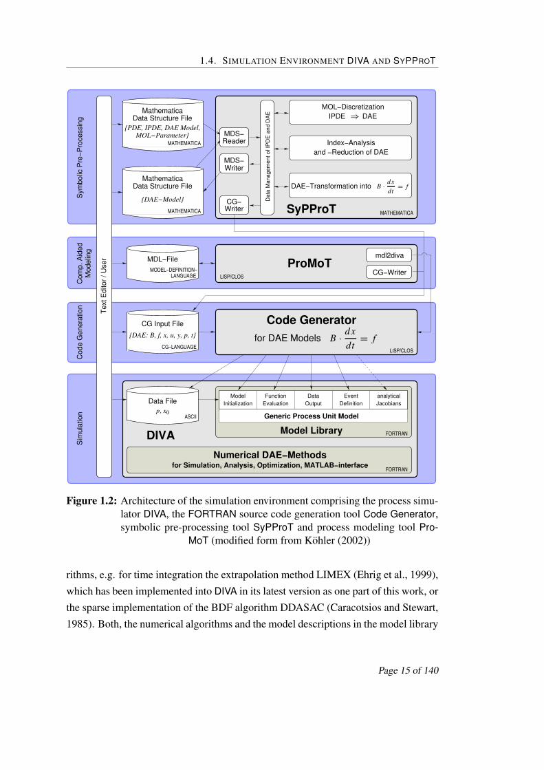
1.2 Architecture of the simulation environment comprising the processsimulator DIVA, the FORTRAN source code generation tool Code

Generator, symbolic pre-processing tool SyPProT and process mod-eling tool ProMoT . . . . . . . . . . . . . . . . . . . . . . . . . . . . 15

2.1 Process flowsheet of the tubular production process of LDPE . . . . . 21

2.2 Cross section of the tubular reactor . . . . . . . . . . . . . . . . . . . 22

2.3 Symbolic scheme of a termination by disproportion (2.7) . . . . . . . 24

2.4 Reaction scheme for the back-biting reaction (2.12), that leads toshort-chain branches (here with a butyl branch). . . . . . . . . . . . . 26

2.5 Reaction scheme for the β-scission (2.13) leading to an unsaturatedend. . . . . . . . . . . . . . . . . . . . . . . . . . . . . . . . . . . . 26

2.6 Sketch for the momentum balance of the reactor inner tube. . . . . . . 28

2.7 Cut out of the tubular reactor with heat fluxes for the energy balanceequation of the wall . . . . . . . . . . . . . . . . . . . . . . . . . . . 32

2.8 Cut out of the tubular reactor with heat fluxes for the energy balanceequations (if a separate energy balance for the reactor wall is included) 37

2.9 Temperature profiles, the mass fractions of monomer and polymer andthe melt flow index at steady state conditions . . . . . . . . . . . . . 53

2.10 Zeroth, first and second moments of the chain length distributions. . . 54

2.11 The weight fractions of initiator and their radicals. . . . . . . . . . . . 55

ix

LIST OF FIGURES

2.12 Temperature profiles and the mass fractions of monomer and polymerat steady state conditions using different discretization schemes andgrid points . . . . . . . . . . . . . . . . . . . . . . . . . . . . . . . . 56

2.13 Temperature profiles and the mass fractions of monomer and polymerat steady state conditions using different discretization schemes andgrid points . . . . . . . . . . . . . . . . . . . . . . . . . . . . . . . . 59

2.14 Movement of grid nodes during the startup of the tubular reactor . . . 60

2.15 Flowsheet representation of the simple mathematical model . . . . . . 66

3.1 Comparison of steady state simulation results from Luposim T andDIVA – temperatures, monomer and polymer weight fractions . . . . . 74

3.2 Comparison of steady state simulation results from Luposim T andDIVA – Nusselt number in the tubular reactor. . . . . . . . . . . . . . 75

3.3 Comparison of steady state simulation results from Luposim T andDIVA – properties of the dead polymer distribution and the melt flowindex. . . . . . . . . . . . . . . . . . . . . . . . . . . . . . . . . . . 77

3.4 Comparison of steady state simulation results neglecting the energybalance for the wall and including it – temperatures and weight frac-tions of monomer and polymer. . . . . . . . . . . . . . . . . . . . . . 78

3.5 Comparison of steady state simulation results neglecting the energybalance for the wall and including it – weight fractions of initiatorand their radicals . . . . . . . . . . . . . . . . . . . . . . . . . . . . 79

3.6 Comparison of dynamic simulation results neglecting the energy bal-ance for the wall and including it – temperature and weight fractionsof monomer and polymer . . . . . . . . . . . . . . . . . . . . . . . . 80

3.7 Profiles of process variables during startup operation, plotted over thereactor length . . . . . . . . . . . . . . . . . . . . . . . . . . . . . . 82

3.8 Comparison of time constants for different startup strategies of thetubular reactor . . . . . . . . . . . . . . . . . . . . . . . . . . . . . . 84

3.9 Influence of disturbances on the outlet temperature – without recycles 85

3.10 Influence of disturbances on the melt flow index – without recycles . . 86

3.11 Influence of the recycles on the time constant of the tubular reactor . . 88

3.12 Influence of disturbances on the outlet temperature – with recycles . . 89

Page x of 140

LIST OF FIGURES

3.13 Influence of disturbances on the melt flow index – with recycles . . . 913.14 Comparison of the steady state reactor temperature profile of the sim-

ple and the rigorous model . . . . . . . . . . . . . . . . . . . . . . . 943.15 Thermal runaway of the simple model . . . . . . . . . . . . . . . . . 953.16 Stability and bifurcation diagram . . . . . . . . . . . . . . . . . . . . 97

4.1 Graphical representation of the objective function for load changes . . 1014.2 Measures of a distribution . . . . . . . . . . . . . . . . . . . . . . . 1024.3 Sensitivities of initiator feed flow rates with respect to 81, 82 and 83 1074.4 Sensitivities of feed parameters with respect to 81, 82 and 83 . . . . 1084.5 Sensitivities of coolant feed temperatures with respect to 83. . . . . . 110

Page xi of 140

LIST OF FIGURES

Page xii of 140

List of Tables

1.1 Investment and running costs comparison of the autoclave and tubularreactor process (¤/t , Whiteley et al. (1998)). . . . . . . . . . . . . . 6

1.2 Low-density, linear low-density and high-density polyethylene pro-duction capacities in 103t per year in 1995 (Whiteley et al., 1998) . . 7

1.3 Some physical properties of low-density polyethylene. . . . . . . . . 9

2.1 Comparison of simulation times tdisctdisc,re f

on a standard with an AMDAthlon™ 64 Processor 3500+ and 1G B RAM. . . . . . . . . . . . . 59

2.2 Comparison of model sizes of the tubular reactor – rigorous versussimplified model . . . . . . . . . . . . . . . . . . . . . . . . . . . . 69

2.3 Kinetic rate expressions used in the simple model . . . . . . . . . . . 71

4.1 Sensitivities of feed parameters with respect to the objectives 81, 82

and 83. . . . . . . . . . . . . . . . . . . . . . . . . . . . . . . . . . 109

xiii

LIST OF TABLES

Page xiv of 140

Notation

Arabic Symbols

Symbol Meaning SI-Unit

A area [m2]cp heat capacity [W/(m2 K)]1hreac heat of reaction [J]E radiation energy [J]F force [N]Gr Grashof numberH enthalpy [J]H enthalpy flux [J/s]i component indexI total number of componentsj reaction number indexJ total number of reactionsk reaction constant [kmol/s]M molar mass [kg/kmol]m mass [kg]m mass flux [kg/s]m A mass flux through area A [kg/(s m2)]NC number of componentsNu Nusselt numberp pressure [N/m2]

Continued on next page

xv

NOTATION


Pn number averagePD polydispersityPr Prandtl numberQ energy flux [J/s]r extent of reaction [mol/(kg s)]

radius [m]R overall heat transfer coefficient [K m/W]Re Reynolds numbert time [s]T temperature [K]U inner energy [J]

perimeter [m]v velocity [m/s]V volume [m3]w weight fraction [-]W sensitivity matrixz spatial coordinate [m]

Greek Symbols


α heat transfer coefficient [W/(m2 K)]1 differenceε emissivityγ weight factor in objective function

skewness of the distributionλ heat transport coefficient [W/(m K)]µk k-th statistical momentν stoichiometric indexπ pi


Page xvi of 140

NOTATION


8 objective function [-]σ Stefan-Boltzmann constant [W/(m2 K4)]

variance% density [kg/m3]2 dimensionless temperature [-]τ dimensionless time [-]

grid node concentrationζ pressure drop coefficient

Abbreviations

Symbol Meaning

BC boundary conditionDAE differential and algebraic equationDB double bondHDPE high-density polyethyleneIC initial conditionIUPAC International Union of Pure and Applied ChemistryLC B long chain branchingLDPE low-density polyethyleneLLDPE linear low-density polyethyleneMFI melt flow indexPDAE partial differential and algebraic equationPE polyethyleneSC B short chain branching

Components

Symbol Meaning

I initiatorContinued on next page

Page xvii of 140

NOTATION

Symbol Meaning

M monomerP dead polymerR radical, living polymerX modifier

Subscripts

Symbol Meaning

0 initial conditionamb ambienceA flux, applied through cross section with area A

air airβ β-scissionbb back bitingC coolantex external wallhp high pressure flashi index of chain length

at the inner reactor wallin at inlet conditionsinner at the inner reactor wall (emphasized)ini t between two initiator injectionsiso insulationj index of reactionsliq liquid phasell laminar layerlp low pressure flashm logarithmic meanM monomerν index for initiators


Page xviii of 140

NOTATION

Symbol Meaning

o at the outer reactor wallouter at the outer reactor wall (emphasized)p propagationrad radialreac reactionrem reminder of the tuberes residence timeR friction

reactorR X modifier radicalsec secondary living polymerst steelsl slime layertc termination due to combinationtd termination due to disproportionth thermaltr transfervap vapor phaseW wallX modifier

Superscripts

Symbol Meaning

P dead polymerR primary living polymerR,sec secondary living polymer

Page xix of 140

NOTATION

Page xx of 140

German Abstract

Im Vordergrund der vorliegenden Arbeit steht die Herleitung eines geeigneten dyna-mischen Modells für die nichtlineare Analyse des Produktionsprozesses von Hoch-druck-Polyethylen (low density polyethylene = LDPE). Das mathematische Modellwird anschliessend verwendet, um Prozessführungsstrategien zu untersuchen. Dabeistehen die Optimierung von Spezifikations- und Lastwechseln sowie die Stabilisie-rung der Arbeitspunkte gegenüber unvorhergesehenen Störungen im Fokus. DerartigeStörungen können schlimmstenfalls durch thermische Zersetzung sogar zum Durch-gehen des Reaktors führen.

Das dynamische Modell der Hochdruck-Polymerisation von LDPE wird ausge-hend von dem Verfahrensdiagramm (Abb. 2.1) hergeleitet. Dabei wird neben einemdetaillierten Reaktionsschema auch eine Energiebilanz für die dicke innere Reaktor-wand des Rohrreaktors berücksichtigt. Um das Gleichungssystem mit dem am Institutfür Systemdynamik und Regelungstechnik (Universität Stuttgart) entworfenen und amMax-Planck-Institut für komplexe technische Systeme weiterentwickelten Prozesssi-mulator DIVA lösen zu können, wird das örtlich verteilte Modell wird mit Hilfe des inMathematica implementierten symbolischen Vorverarbeitungswerkzeuges SyPProT

in ein Modell überführt, welches nur noch aus Differential- oder algebraischen Glei-chungen besteht. Dabei wird eine finite Differenzen-Methode verwendet, welcher ent-weder ein ortsfestes oder ein bewegliches Gitter zu Grunde liegt.

Das erste Modul des Rohrreaktors wird anhand von Daten des Kooperationspart-ners validiert. Zur Validierung wird ein ortsfestes, sehr hoch auflösendes Gitter ver-wendet. Die Übereinstimmung zwischen den Daten und den Profilen aus einer statio-nären Simulation ist sehr gut. Allerdings ist ein Gesamtmodell mit einem derart hochauflösenden Gitter nicht auf einem gewöhnlichen Standard-PC numerisch lösbar. Da-her werden Simulationsresultate des hoch auflösenden Gitters mit denen verglichen,

1

GERMAN ABSTRACT

welche weniger Gitterpunkte verwenden. Dabei steigt der Diskretisierungsfehler mitder Verringerung der Anzahl der Gitterpunkte. Durch die Verwendung eines adaptivenanstelle eines ortsfesten Gitters kann allerdings bei deutlich weniger Stützstellen einvergleichbares Ergebnis erzielt werden. Daher wird in allen folgenden Simulationendie adaptive Diskretisierungsmethode verwendet.

Wie schon im vorhergehenden Abschnitt erwähnt, berücksichtigt das detaillierteModell die axiale und radiale Wärmeleitung in der Rohrwand. Damit wäre es al-lerdings notwendig, die Rohrwand auch in radialer Richtung zu diskretisieren. Umdas Modell dadurch nicht zusätzlich erheblich zu vergrößern, wird die innere Reak-torwand in zwei Schichten gleicher Dicke geteilt. Die Temperatur in der Mitte wirdals eine gemittelte Wandtemperatur betrachtet und die radiale Wärmeleitung kannim Wärmeübergangskoeffizienten berücksichtigt werden. Die Dicke der Wand be-einflusst die stationären Simulationsergebnisse nur geringfügig, wohingegen sich dieZeitkonstanten um einen Faktor in der Größenordnung einer Dekade verändern.

Obwohl die Simulationsdauer für einzelne Szenarien beträchtlich ist, erweist sichdas detaillierte Modell ohne Materialrückführung robust gegenüber allen aufgepräg-ten sprungförmigen Störungen. Ein Schließen der Rückführungen führt jedoch dazu,dass das Gesamtsystem instabil werden kann. Dieses Verhalten soll durch eine nicht-lineare Modellanalyse untersucht werden, aber das detaillierte Modell kann auf Grundseiner Größe mit den dafür in DIVA zur Verfügung stehenden Methoden nicht gelöstwerden. Daher wird ein vereinfachtes Modell für diese Betrachtungen herangezogen.Dieses Modell enthält zahlreiche Annahmen, welche die Anzahl der Gleichungen re-duzieren, z.B. entfällt durch eine konstante Kühltemperatur die Energiebilanz für dasKühlmedium, außerdem entfallen vier partielle Differentialgleichungen für Initiato-ren bzw. deren Radikale, etc.. Trotz der z.T. erheblichen Vereinfachungen gibt dasreduzierte dynamische Modell qualitativ das Verhalten des detaillierten wieder. Le-diglich im Reaktoraustritt kommt es zu größeren Abweichungen, welche durch dieAnnahme eines konstanten Wärmedurchgangskoeffizienten erklärbar sind.

Die nichtlineare Analyse des vereinfachten Modelles kann die Resultate andererForschungsgruppen übereinstimmend wiedergeben. Durch eine Parameterfortsetzungkann neben Betriebsbereichen mit bis zu fünf stationären Betriebspunkten auch ei-ne Hopf-Bifurkation gefunden werden. Jedoch überschreitet dieser Betriebspunkt denrealen Betriebsbereich der Anlage. Nichtsdestoweniger kann der Hopfpunkt im Rah-

Page 2 of 140

GERMAN ABSTRACT

men von weitergehenden Untersuchungen als Ausgangspunkt für eine Zweiparame-terfortsetzung herangezogen werden.

Für eine dynamische Optimierung ist die Sensitivitätsanalyse ein wichtiger ersterSchritt. Diese wird mit dem detaillierten Modell durchgeführt, um die wesentlichenEinflußgrößen auf den Prozess zu ermitteln. Dazu werden drei Zielfunktionen defi-niert, hinsichtlich derer der Einfluss der Parameter untersucht wird. Resultat dieserUntersuchung ist, dass zwar für eine nichtlineare Analyse Momente höherer Ord-nung vernachlässigt werden dürfen, dies jedoch für eine Optimierung nicht sinnvollerscheint. Denn die physikalischen Eigenschaften des Polymers hängen von der Ket-tenlängenverteilung ab und wesentliche Kenngrößen dieser Verteilung lassen sich aufder Basis von Momenten ableiten.

Es bleibt festzuhalten, dass selbst mit derzeitigen Standard-PCs die dynamischeSimulation eines rigorosen Modells der LDPE Produktion im Rohrreaktorverfahrenein sehr anspruchsvolles numerisches Problem darstellt. Vielleicht könnte die Wahleines anderen Simulators das Problem der großen Rechenzeiten lösen, jedoch müs-sen dann evtl. Abstriche hinsichtlich Optimierung und nichtlinearer Analyse gemachtwerden. Nichtsdestotrotz kann das in dieser Arbeit abgeleitete detaillierte Modell sehrgut als Ausgangsbasis verwendet werden, um daraus für die jeweilige Applikationgeeignete einfachere Modelle zu gewinnen, z.B. für dynamische Optimierungen odermodellprädiktive Regelungsaufgaben.

Page 3 of 140

GERMAN ABSTRACT

Page 4 of 140

Chapter 1

Introduction

A journey of a thousand miles begins with a single step.

– Confucius

The primary objective of this work is the development of a suitable dynamic model forthe analysis of a polyethylene production plant. The mathematical model is used for asuccessive study of process control strategies. Most important tasks in this regard areoptimization of grade or load changes and stabilization of steady state behavior dueto unforeseen disturbances. In worst case, such disturbances may render the reactorunstable, i.e. might lead to thermal runaway. So, in this chapter, an overview ofthe development of polyethylene production and a summary of the most importantpolyethylene properties is given (Sec. 1.1 and 1.2).

Thereafter, a literature survey is presented followed by a short introduction intothe simulation environment that is used in this work (Sec. 1.4). A brief scope closesthis chapter (Sec. 1.5).

1.1 Polyethylene Production – Past to Present

A very detailed history of development of the different types of polyethylene can befound e.g. in Plastics and Rubber Institute (1983a,b); Seymour and Cheng (1986);Whiteley et al. (1998).

Polyethylene is a polymer that is produced from the monomer ethene. The name ofthe polymer is derived from the non-IUPAC (International Union of Pure and Applied

5

CHAPTER 1. INTRODUCTION

Chemistry) monomer name ethylene (≡ ethene).

The discovery of polyethylene (PE) was the result of experiments carried out toevaluate the effort of applying high pressures on chemical reactions. In 1933, ethy-lene gas was compressed to 1400 bar . As a result, a white solid was formed in thevessel and that solid turned out to be Low-Density PolyEthylene (LDPE). Later it wasshown that the presence of traces of oxygen caused the polymerization and that largeramounts of oxygen would lead to heavy explosions. A pilot plant with a small reactorproduced small amounts of LDPE with at that time interesting product properties.

The first commercial plant started its production in 1939. In World War II, LDPEwas used as a flexible, low density coating and insulating material for electrical ca-bles. E.g. as an underwater cable coating or more important from a strategic militarypoint of view as a critical insulating material for such applications as radar insulation.Because of its light weight, radar equipment was easier to carry on a plane, whichallowed the out-numbered Allied aircrafts to detect German bombers. By the end ofthe war, England’s production of PE was 20 times higher than before the war.

In the beginning of the industrial production of low-density polyethylene, poly-merization was started only by using free radical initiators leading to partially crys-talline polymers. The degree of the crystalline structure was determined by measuringthe density. The process was carried out at high pressure and high temperatures. Athigher temperatures one has to deal with side reactions which lead to a branched poly-mer and thus the densities were lower than what could be expected of a completelyamorphous and crystalline polyethylene.

Later developments led to a process involving catalysts. Such a process could becarried out at lower pressure and lower temperatures and hence the densities were

Process Autoclave TubularCapacity (103t/a) 117 200Capital cost (106 ¤) 70 96Production cost 565 544Depreciation 71 59Total costs 636 603

Table 1.1: Investment and running costs comparison of the autoclave and tubular re-actor process (¤/t , Whiteley et al. (1998)).

Page 6 of 140

1.1. POLYETHYLENE PRODUCTION – PAST TO PRESENT

higher (High-Density-PolyEthylene). High-density polyethylene has a density thatranges from 0.94 to 0.97 kg

m3 . Its molecules have an extremely long carbon back-bone with no side groups. As a result, these molecules align into more compactarrangements, accounting for the higher density of HDPE. High-density polyethyleneis stiffer, stronger, and less translucent than low-density polyethylene.

The original process for the LDPE production was based on an autoclave reactor.There, the hot reactants mix with the cold incoming ethylene and keep the processstable. Later on, the process involving the tubular reactor was developed. This processproduced LDPE with a consistent molecular weight. Still, both production processesare commercially used, and although they are operated at very high pressures, some ofthese reactors have been in service for many years. Not only LDPE, but also LLDPE(Linear LDPE) can be produced in the high-pressure process.

The physical properties of LDPE produced in autoclave reactors differ signifi-cantly from those of the tubular reactor process. Autoclave LDPE products are con-sidered to be the products of choice for extrusion coating applications. On the otherhand, LDPE resins produced using tubular reactors are more suitable for extrudedfoam applications. Hence, depending on the application, the reactor type has to bechosen (Auger and Nguyen, 2001). If the application allows both types, then one ad-vantage of autoclave reactors is that they have lower investment costs, based on thecost of the reactor system. On the other hand, variable costs for tubular reactors areslightly lower (Tab. 1.1).

N. America Europe Japan Rest Total

LDPE 3891 7701 1444 4210 17246LLDPE 4422 1948 1059 3728 11157HDPE 6198 4881 1024 4715 16891

Total 14511 14530 3527 12653 45221Table 1.2: Low-density, linear low-density and high-density polyethylene production

capacities in 103t per year in 1995 (Whiteley et al., 1998)

Since it can be produced within a very broad range of both different grades anddifferent manufacturing processes, polyethylene has now become one of the majorplastic worldwide. Summing up the most important types of polyethylene, in particu-

Page 7 of 140


lar low-density, linear low-density and high-density polyethylene, the annual produc-tion rate is ≈ 45 106t in 1995, see Table 1.2. Such a high production rate also implies,that any failure in the production process is very costly. Failure includes also up- ordownstream processing.

In Germany, the vast majority of steam crackers is located in the Rhine valley inthe Köln/Wesseling/Gelsenkirchen area. But also Münchsmünster and Burghausenare very important production sites. Because of their island position (far in the south,far-off from the major consumers except of Wacker-Chemie), it is planned to built anethylene pipeline from there to the production sites of BASF in Ludwigshafen (seeEthylen-Pipeline Süd GbR (2006)). This pipeline should bring more process relia-bility and flexibility to both, the ethylene production sites and the ethylene process-ing sites, because the produced ethylene has to be processed further on immediately.Hence a failure in the ethylene production would always result in a failure of thewhole production site and vice versa.

1.2 Physical Properties

Usually polyethylenes are characterized by their density or by the Melt Flow Index(MFI). The MFI test was initially developed for LDPE as a measure for the meltcharacteristic under conditions related to its processing. Low-density polyethylenehas a density ranging from 0.91 to 0.93 kg

m3 . The molecules of LDPE have a carbonbackbone with side groups of four to six carbon atoms attached randomly along themain backbone. LDPE has a high number of long- and short-chain branches whichresults in a lower tensile strength and increased ductility. It is a whitish solid that isflexible.

LDPE combines electrical insulation properties with toughness, flexibility, light-ness and inertness. Inertness means here that it is resistant to acids, alcohols, basesand esters. Moreover it is easily weldable.

Some of the most important physical properties are given in Tab. 1.3. The corre-lation of important properties to process variables is depicted in Fig. 1.1. As one cansee from there, the operation conditions are of major importance for the properties ofthe final product. The plot in the top left position shows that from a conversion pointof view, the higher temperature and pressure in the process, the higher the conversion.

Page 8 of 140

1.3. LITERATURE SURVEY

Property ValueMelting point 100÷120 ◦CUtilization temperature −50.0÷ [50.0 . . .80.0] ◦CGlass transition temperature ≈ −40 ◦CDensity 0.91÷0.93 kg

m3

Tensile Strength 5÷25 MPaViscosity 17 kPa · sThermal conductivity (at 23◦C) 0.33 W

K mSpecific heat 1900-2300 J

kgKTransparency translucentChemical resistance against acids, solvents and alkalis

Table 1.3: Some physical properties of low-density polyethylene.

But if one also looks at the other three diagrams, then it is clear that operating thisprocess is always a balancing act between conversion and properties and also betweenproperties amongst each other.

The predominant uses of both LDPE and LLDPE is for films, e.g. for packagingin food industry because of its translucency and inertness. But these films are notall for packaging purposes, e.g. by welding one end bags are produced directly fromthe film. Apart from these packaging applications also of heavy duty sacks are madeout of LDPE or LLDPE. Moreover it can be used e.g. for sealing membranes in civilengineering constructions or for shrink-wrap, squeezable food bottles or as insulationmaterial for wires and cables.

1.3 Literature Survey

As indicated by Tab. 1.2, LDPE is one of the most often produced polymers in theworld. Hence also the amount of publications dealing with the kinetics and physi-cal properties as well as the production of low-density polyethylene is enormous. Agood overview on the polymerization of olefins in general is given in Kiparissideset al. (1993); Ray (1983) and Whiteley et al. (1998). There the most important re-action steps, the different types of PE as well as the main production processes areintroduced. Ray (1972) focuses on the mathematical modeling of polymerizationreactors in general. This review lists different techniques for the calculation of molec-

Page 9 of 140


ular weight distributions. One of these techniques is the introduction of statisticalmoments, and a summary lists properties of distributions, which can be expressedin terms of those moments, e.g. number average chain length or the variance ofthe number average chain length distribution σ 2. Congalidis and Richards (1998);Schuler (1981) and Kiparissides (1996) focus on the control of polymerization pro-cesses. A general solution to both control and optimization is an accurate mathe-matical model of the process, an appropriate set of control/optimization parameters,a suitable objective and an efficient numerical method for the solution of the specificproblem. In particular, the definition of the objective function is not always easy in thesense that some controlled variables may react in opposite directions to variations ofa control/optimization parameter. Moreover, the resulting problems are challengingto solve numerically.

conv

ersi

on temperature

pressure m

elt f

low

inde

x

temperature

pressure

haze

temperature

pressure

dens

ity

temperature

pressure

Figure 1.1: Relationship of physical properties to process variables, such as temper-ature or pressure (Meyers, 2004)

Page 10 of 140


Publications of Luft (1979, 2000) give a good overview on the production of high-density polyethylene in both lab-scale and industrial processes. In particular, due tothe rise in energy costs, a rise in operating pressure is now obsolete, even though thisinfluences product properties for some applications positively. However, in the highpressure process, there is an enormous effort to save energy costs. This also implieswell designed separators, since the degree of separation is higher, the lower the flashpressure is taken. Hence, also the solubility of monomer in the polymer melt has beenstudied intensively, e.g. Bokis et al. (2002); Koak et al. (1999); Liu and Hu (1998);Orbey et al. (1998). But for this work, a two parametric equation is fitted to measureddata. Not only the phase equilibrium, but also all reaction rates have been subject ofresearch projects. Luft et al. (1978) investigated the decomposition rates of differentinitiators for high pressure polymerizations. They reported a pressure dependency ofthose rates which they expressed in terms of activation volumes in the reaction rate.

Beuermann and Buback (1997) primarily addressed the propagation and termina-tion rate coefficients of homo-polymerizations. Their special emphasis has been ona conversion dependent termination rate of low-density polyethylene at pressures upto 3000 bar and temperatures up to 300◦C . They also reported that limitations ofprevious simulation studies mainly resulted from limited availability and reliabilityof kinetic data even for homo-polymerizations. Other literature, e.g. by Luft et al.(1982) reported that initiator types have no effect on long- or short-chain branching,whereas higher temperatures promote the formation of both branching types. More-over also the reactor geometry influences the long-chain branching, since this changesthe temperature distribution in the reactor.

Buback et al. (2000) reported a termination rate that is dependent on the chainlength and additionally Busch (2001a) used a reaction rate for the transfer reactionto polymer which is dependent on the chain length. Thereby a better estimate forpropagation reaction could be derived. In these studies and also in Busch (2001b),simulations using Predici® supported the experiments.

According to Hutchinson and Fuller (1998), β-scission and long-chain branchingare the reaction steps, that are very important for the physical properties of the pro-duced polymer. Additionally, these reactions prevent gel formation even though onthe one hand the rate coefficients of these reactions are small compared to propaga-tion and on the other hand only 2.4% of all secondary radicals undergo intramolecular

Page 11 of 140


β-scission.

Lorenzini et al. (1992a,b) fitted the kinetic parameters of a very detailed reactionscheme in an autoclave reactor. They reported, that the application of a quasi steadystate assumption is problematic for free radicals in the tubular reactor process, becauseof rapid temperature changes occurring along the axis.

Various publications use different modeling methods for the simulation of poly-merization reactors. In particular, Tsai and Fox (1996) used computational fluiddynamics for three-dimensional simulations of the polymerization of low densitypolyethylene in a tubular reactor at the nominal operating point. Although their ki-netics is rather simple, also they reported, that depending on the kinetics the quasisteady state assumption sometimes fails. For some cases, they found an error largerthan 100 % for monomer conversion, if this assumption is used. Moreover also reac-tor geometry and operating parameters have large influence on monomer conversion.Read et al. (1997) confirmed this result and concluded, that there is a need for anoptimization of operating parameters. Also Zhou et al. (2001) used CFD simulationsfor the solution of a two-dimensional tubular and a three-dimensional autoclave reac-tor. Additionally their models provided information on the physical properties of thepolymer, such as polydispersity or mean of the molecular weight distribution.

Zacca et al. (1997) applied population balances to the model of an autoclave reac-tor and examined effects of the residence time distribution. According to their find-ings, this plays a significant role in the formation of the physical properties of thehomo-polymer. A brief overview on the different modeling and simulation strategiescan be found in Bartke and Reichert (1999).

Publications, dealing with steady state models of the tubular reactor process arenumerous. Here only a few examples are listed. Zabisky et al. (1992) derived a steadystate model, using a very sophisticated reaction scheme with additional initiation us-ing oxygen. Yet, none of the rate coefficients was depending or either chain length orconversion. A similar reaction scheme was used (by the same authors) in Chan et al.(1993) for an autoclave reactor. Kiparissides et al. (1996) derived a steady state modelfor on-line parameter estimation, such that the model captures the actual reactor op-eration. Lacunza et al. (1998) investigated on the influence of the overall heat transfercoefficient. They reported, that correct estimates of the heat transfer coefficient area major issue for predicting the plant behavior using rigorous mathematical models.

Page 12 of 140


In Mähling et al. (1999) results of the reference of the rigorous model in this workare published. There the simulations are coupled to Predici®, in order to derive themolecular weight distribution.

The first dynamic mathematical model is reported in Gilles and Schuchmann(1966) using a simple reaction scheme (only the main reactions for free radical poly-merizations) and constant parameters such as overall heat transfer coefficients, densityetc. As a first publication in a series, Brandolin et al. (1996) derived a rather detailedsteady state model. However, also this model shows no reaction rate depending onchain length or conversion. Moreover the overall heat transfer coefficient is constant.Later on, the complex steady state model has been converted into a rather simple dy-namic model, still using constant parameters, e.g. for heat transfer. The simple modelhas then been used for simulation and optimization results in several publications(Asteasuain et al., 2000, 2001; Cervantes et al., 2000).

Additionally, Ray (1981) investigated the dynamic behavior of polymerizationreactors. Runaway, multiple steady states and autonomous oscillations are reportedthere for CSTRs and autoclave reactors. According to Villa et al. (1998) and Ray andVilla (1999), the nonlinear behavior depends on the type of polymer and its kinetics,the type of reactor, the heat removal system and the phase behavior. However, theseresults have only been investigated on autoclave or continuous-stirred tank reactors.

Hence, despite of various sources in literature, only few dynamic models are avail-able in literature so far, which additionally lack some important features, that are re-ported to have significant influence (e.g. a variable overall heat transfer coefficient).One reason might be, that in former days, the plants have been built as single-productplants. However, nowadays, due to technical progress, polymers can be produced indifferent grades in the same plant just by changing the operating conditions. So theseplants are not only operated in steady state regimes, they undergo frequent dynamictransitions between these steady states. In fact, in modern tubular reactor processes,up to 15 different grades may be produced. In order to simulate and optimize gradechanges, a rigorous dynamic model has to be developed.

The level of detail is needed to have a physical insight to the very complex pro-cess, that not only incorporates many components but is also operated at extremeconditions, such as high pressure or high temperature, which is quite close to glasstemperature. Since dynamical aspects are the main focus of this work, the influence

Page 13 of 140


of the tube wall cannot be neglected. Because almost all models available in litera-ture are of steady state type, this effect has never been studied so far, although theremight occur some interesting unexpected behavior, as this reaction is highly exother-mic. Eigenberger (1974) reported such behavior for highly exothermic reactions. Ithas been stated, that the effect of the heat accumulation causes excess temperaturesto occur for lowering the feed temperature or raising the feed flow rate. In fixed-bedreactors Mangold et al. (1998, 2000b) observed similar effects. Since in these publi-cations gas phase reactions have been studied, the effects become much more visible.

Of course, the level of detail required for such purposes like optimization, alsocauses difficulties. Deriving the mathematical model equations from first principles,one ends up with a considerable number of partial differential and algebraic equations(PDAEs). The simulator DIVA, which is briefly introduced in the Sec. 1.4, is onlycapable to solve differential and algebraic equation (DAE) systems. Hence the systemof PDAEs has to be transformed into a set of DAEs, which is done by a Method ofLines approach utilizing a moving grid (Köhler, 2002; Köhler et al., 2001; Wouweret al., 2001). Moving grid means, that the grid points are not fixed to some location,but the position of the grid points may change with respect to a monitored function.This enables one to reduce the number of grid points, while the resolution in regionsof large gradients is still reasonable.

1.4 Simulation Environment DIVA and SyPProT

In this section, the simulation environment which is used throughout this work is in-troduced. As one can observe from Fig. 1.2, this environment integrates the four maintools, the process simulator DIVA (Holl et al., 1988; Kröner et al., 1990), the pre-processing tool for differential and algebraic equations Code Generator (Räumschüs-sel et al., 1994), the symbolic pre-processing tool for integro partial differential andalgebraic equations SyPProT (Köhler, 2002) and the process modeling tool ProMoT

(Tränkle, 2000; Waschler et al., 2006), which presently supports a DAE descriptionof the mathematical model implementation.

The process simulator DIVA integrates different numerical methods for the sim-ulation, analysis and optimization of large nonlinear differential algebraic equationsystems. Therefore it utilizes very efficient state-of-the-art sparse numerical algo-

Page 14 of 140

1.4. SIMULATION ENVIRONMENT DIVA AND SYPPROT

FORTRAN

FORTRAN

LISP/CLOS

InitializationModel

EvaluationFunction Data

Output DefinitionEvent analytical

JacobiansData File

ASCII

Numerical DAE−Methodsfor Simulation, Analysis, Optimization, MATLAB−interface

Model Library

Generic Process Unit Model

for DAE Models

Code Generator

DIVA

CG−LANGUAGE

CG Input File

{DAE: B, f, x, u, y, p, t}

Text

Edi

tor /

Use

r

MathematicaData Structure File

{DAE−Model}

MOL−Discretization

Index−Analysisand −Reduction of DAE

MATHEMATICASyPProT

IPDE DAE

DAE−Transformation into

Reader

WriterCG−

MDS−Writer

MDS−

MATHEMATICA

MathematicaData Structure File

MOL−Parameter}{PDE, IPDE, DAE Model,

MATHEMATICA

Dat

a M

anag

emen

t of I

PD

E a

nd D

AE

MDL−File

LISP/CLOS

mdl2diva

CG−WriterProMoT

LANGUAGEMODEL−DEFINITION−

Com

p. A

ided

Mod

elin

gS

ymbo

lic P

re−P

roce

ssin

gC

ode

Gen

erat

ion

Sim

ulat

ion p, x0

B ·dxdt

= f

⇒

B ·dxdt

= f

Figure 1.2: Architecture of the simulation environment comprising the process simu-lator DIVA, the FORTRAN source code generation tool Code Generator,symbolic pre-processing tool SyPProT and process modeling tool Pro-

MoT (modified form from Köhler (2002))

rithms, e.g. for time integration the extrapolation method LIMEX (Ehrig et al., 1999),which has been implemented into DIVA in its latest version as one part of this work, orthe sparse implementation of the BDF algorithm DDASAC (Caracotsios and Stewart,1985). Both, the numerical algorithms and the model descriptions in the model library

Page 15 of 140


are implemented in FORTRAN. The mathematical models of individual process unitsare represented in the form of linear-implicit differential and algebraic equations witha differential index ≤ 1

B(x,p,u, t)x = f(x,p,u, t) (1.1)

with the initial conditions

x(t = t0) = x0. (1.2)

In general, B ∈ IRNx×Nx is a not necessarily regular left-hand side matrix, and f ∈ IRNx

is the right-hand side function vector. x ∈ IRNx is the vector of the state variables withinitial values x0, where Nx is the total number of states. p ∈ IRNp and u ∈ IRNu areparameter and input variables.

Since the coding of individual process units in FORTRAN is very inconvenient, theCode Generator allows a symbolic description of the mathematical model equationsand automatically converts them into efficient FORTRAN code. Still the model must

be represented as DAE system. Nevertheless, the Code Generator is both the interfaceto DIVA for users and the interface for more advanced tools, such as SyPProT andProMoT.

ProMoT is a modeling tool for object-oriented and equation-based modeling ofarbitrary equation systems. It contains modeling entities that represent the structureof unit models, in particular its model equations and interface definition. By aggrega-tion and inheritance knowledge bases may be designed, whose modeling entities (theprocess units) have standard interfaces, are well documented and hence suitable fordirect reuse and refinement. ProMoT either generates a Code Generator input file,or directly accesses the Code Generator. However, ProMoT also does not supportdistributed models.

This gap is closed by the package SyPProT . This package symbolically trans-forms a given system of integro partial differential and algebraic equations into adiscretized set of ordinary differential and algebraic equations. The latter is then con-verted into a format the Code Generator supports. So far, ProMoT and SyPProT arenot connected to each other, even though both would benefit from the advantages of

Page 16 of 140

1.5. OUTLINE OF THIS WORK

the other. Here, because of the nature of the rigorous model equations, the symbolicpre-processing tool SyPProT is used for the implementation of the model.

1.5 Outline of this Work

Each chapter starts with a more detailed introduction on its scope. Hence, here onlya brief overview of this work is given. At first, in Chap. 2, the production process isintroduced, and the detailed dynamical model for all involved process units will bederived and presented. The partial differential equation system of the rigorous math-ematical model is transformed into a system of differential and algebraic equationsusing an Adaptive Method of Lines. Moreover, a second, simpler model is presentedand discussed in this chapter. The simple model is used for the nonlinear analysis ofthe system. Simulation results are presented in Chap. 3, which is divided into threeparts. The first two parts present steady-state (Sec. 3.1) and dynamic (Sec. 3.2) sim-ulation results of the detailed model. The third part (Sec. 3.3) shows the nonlinearanalysis using the simple model. Chap. 4 gives an outlook on dynamic optimizationof the process, therefore a sensitivity analysis is used to identify both, suitable ob-jectives and important optimization parameters. Finally, a summary will be given inChap. 6 and the interested reader may look in detail at all model equations (App. B)and some additional remarks on the Adaptive Method of Lines in App. C.

Page 17 of 140


Page 18 of 140

Chapter 2

Modeling

No human investigation can be called real science if it cannot be demon-

strated mathematically.

– Leonardo da Vinci

In this chapter, one of the main parts of this work is introduced, the derivation ofthe rigorous dynamic mathematical model. At first, a detailed overview of the pro-duction process involving a tubular reactor is given (see process flowsheet in Fig. 2.1).Then, in Sec. 2.2, the reaction scheme and the detailed distributed model of the tubularreactor are introduced. To include the heat capacity of the thick reactor wall, withoutincreasing the model size drastically, a simple discretization scheme is proposed toaccount also for the radial heat transfer. The partial differential and algebraic equa-tions are transformed into a system of ordinary differential and algebraic equationsusing a Method of Lines approach. Both, simulations of only the tubular reactor withan equidistant and an adaptive grid are compared to each other and the moving gridis chosen for the remainder of this work since it offers a reasonable compromise be-tween model size and accuracy. In Sec. 2.3, the mathematical models of the peripheralunits, such as compressors, flash units or recycle lines are shown. These units are de-scribed by ordinary differential and algebraic equations. For the nonlinear analysis,in addition to the rigorous dynamic model, a simpler dynamic model of the tubularreactor is presented, which includes also a simplified reaction scheme.

19

CHAPTER 2. MODELING

2.1 Process Description

LDPE can be produced in either an autoclave or a tubular reactor. As mentioned inChap. 1, both types are commercially in use. In this work, only the tubular reac-tor production process is considered. A rough flowsheet of the process is shown inFig. 2.1.

The feed to the plant is fresh monomer (ethylene) together with the modifier thatcontrols the molecular weight. The feed is mixed with the low pressure recycle streamand pre-compressed in a primary compressor to an intermediate pressure of approx.250−300 bar . The outlet of the primary compressor is mixed with the high pressurerecycle and compressed in the hyper compressor to a final pressure of approx. 2000−

3000 bar . The hyper compressor consists of two stages. After the second stagethe ethylene is further heated up for the reaction to take place. The high pressure isrequired since ethylene is gaseous above its critical temperature of 9◦C . At pressuresabove 2000 bar and temperatures higher than 160◦C , the polymer is able to dissolvein the unreacted ethene.

The outlet of the hyper compressor is fed to the main unit of the low-density pro-duction process, the tubular reactor. Right at the inlet of the tubular reactor, a mixtureof three different initiators is injected into the feed stream. These initiators decom-pose selectively with respect to temperature and start the chain growth reaction. Thereaction is highly exothermic and heat is removed by coolant cycles that are operatedco- or counter-current wise. The coolant is kept at two different temperature levels.Usually for removing the heat in the two cooling zones right after an initiator injectionpoint warmer coolant is taken. The next two zones are operated at a lower level, to beable to add fresh initiator at the successive injection point. Since the temperature atthe successive injection points is already at a higher level, only initiators decomposingat intermediate and high temperatures are added there.

The length of a tubular reactor for LDPE production is > 1000 m. Inspite ofthis length, the conversion acchieved in the reactor is only about 25 − 35 %. Hence,unreacted monomer and modifier have to be separated from the product in two flashunits. The unreacted monomer and the modifier are recycled in two recycle lines,which are operated at different pressure levels. There they are cooled down and fedagain to the process at the compressors with corresponding inlet pressure level. The

Page 20 of 140

2.1. PROCESS DESCRIPTION

Sepa

rati

on

Ext

rude

r

Init

iato

rm

ixtu

relo

w,m

ediu

m,h

igh

Hyp

er-

Pre-

com

pres

sor

com

pres

sor

LP

sepa

rato

r

HP

sepa

rato

r

Stor

age

Dry

er

Hea

texc

hang

er

Init

iato

rm

ixtu

rem

ediu

m,h

igh

Init

iato

rm

ixtu

reIn

itia

tor

mix

ture

med

ium

,hig

hm

ediu

m,h

igh

Coo

ling

Coo

ling

Coo

ling

Coo

ling

Hea

texc

hang

erB

oost

er

Eth

ylen

e

Valve Heat exchanger

Rea

ctio

n

Figure 2.1: Flowsheet of the tubular production process of low-density polyethylene

Page 21 of 140

CHAPTER 2. MODELING

polyethylene melt, which still contains minor quantities of ethylene is completelywithdrawn from the plant, and processed downstream further on. The downstreamprocessing involves an extruder for degassing and for inclusion of additives to meetthe final customer requirements. Common additives are dyeing agents, UV-stabilizer(e.g. carbon black), anti-static additives or fire protectors.

As one can see from Fig. 2.1, the plant can be considered as reactor-separatorsystem. Reaction takes place of course in the tubular reactor, whereas the separatorunits are located downstream to recover unreacted monomer from the product. Theunreacted material is recycled in the two recycle lines. For purposes of clarity thereactor section in Fig. 2.1 is shown in a blue box, whereas the separator units areenclosed in a gray box.

In this chapter the model of the plant is derived from first principles using con-servation laws for momentum, mass and energy. All units except the downstreamprocessing units, i.e. the extruders for the incorporation of additives and degassingwill be part of the detailed mathematical model. Starting with the model of the tubu-lar reactor in Sec. 2.2, the model equations of the more peripheral units (compressors(see Sec. 2.3.2) and the flash units (see Sec. 2.3.3)) will be presented. In Sec. 2.4 a

core retrainer

coolant

air gap

inner wall

outer wall

insulation

Figure 2.2: Cross section of the tubular reactor

Page 22 of 140

2.2. DETAILED MODEL OF THE TUBULAR REACTOR

simplified model of the process will be introduced which will enable us to analyze thenonlinear behavior of this reactor-separator system in detail.

2.2 Detailed Model of the Tubular Reactor

A sketch of a cross-section of the tubular reactor is depicted in Fig. 2.2. As one canobserve, the reactor itself consists of three nested tubes, the inner wall, the outer walland the insulation. Moreover, between outer wall and insulation there is an air gapfor additional insulation. In the detailed model, which will be derived in this section,the coolant will flow in the counter-current direction, but in the real process, it ispossible to operate each coolant cycle differently. Although the sketch in Fig. 2.2 isnot provided with a scale, the relations of the different thicknesses are drawn correctly.In particular, the thickness of the inner wall is approximately of the same order as theinner diameter and large compared to the thickness of the outer wall and the insulation.

In the tubular reactor the single-phase ethylene-polyethylene mixture allows thereaction to take place as a free radical initiated polymerization. A detailed explanationof the reaction mechanism is given in the following subsection. Then the model equa-tions are derived and the simplifications are introduced and discussed. Moreover, themodel will be validated and different discretization schemes are compared. Based onthis comparison, an appropriate scheme is selected and used throughout the remainderof this work for all simulations that use the rigorous model of the tubular reactor.

2.2.1 Reaction Mechanism

Both, in a tubular or an autoclave reactor, LDPE is produced by a free radical poly-merization. For free radical polymerizations, the reaction scheme can be divided intotwo parts, the main reactions (Sec. 2.2.1.1), which are characteristic for all free radicalpolymerizations and the side reactions (Sec. 2.2.1.2). Side reactions usually accountfor the structure (linear or branched chains, longer or shorter branches) and hence forthe physical properties of the polymer.

Page 23 of 140

CHAPTER 2. MODELING

C CC C CC C C C C

Figure 2.3: Symbolic scheme of a termination by disproportion (2.7)

2.2.1.1 Main Reactions

The main reactions, which are common to all free radical polymerizations, compriseinitiation, propagation and termination. Therefore free radical donators, such as oxy-gen or peroxides are used to initiate the polymerization. In this work, the reaction isstarted with a mixture of different initiators. Each of them decomposes into radicals ata distinct temperature level. E.g. at the inlet of the tubular reactor, a mixture of threedifferent initiators is used. One decomposes at moderate temperatures, another one atintermediate and the third one only at very high temperatures. Buback (1980) reporteda thermal initiation of ethylene, also leading to radicals. The rate of thermal initiationusually is much lower than the one corresponding to the other initiation reactions.The next main step is the chain growth reaction. In the presence of radicals, newmonomer molecules are added to the reactive end of the radical, forming longer rad-icals, so-called “living polymer”. When the concentration of radicals is high enough,in the third step, the chain growth reaction terminates resulting in “dead polymer”.Two different mechanisms lead to the termination, combination and disproportion. Aschematic sketch of the termination by disproportion reaction is depicted in Fig. 2.3.Since Reac. (2.7) results in two dead polymer chains, one end of the one chain isunsaturated, meaning that there occur double bonds.

The following reaction scheme summarizes the main reactions,

IνkIν

−−−→ 2 RIν initiator decomposition, (2.1)

RIν + Mkp,Iν

−−−→ R1 initiation, (2.2)

RX + Mkp,X


3 Mkth

−−−→ 2 R1 + M thermal initiation, (2.4)

Ri + Mkp

−−−→ Ri+1 propagation, (2.5)

Page 24 of 140


Ri + R jkt,c

−−−→ Pi+ j termination by combination and (2.6)

Ri + R jkt,d

−−−→ Pi + Pj + DB termination by disproportion. (2.7)

In this notation, the index ν is used for the distinction of the different initiators I

(ν = 1,2,3). A higher index means a lower decomposition temperature of the initiator,i.e. initiator 1 decomposes at high, initiator 3 at low temperatures. Moreover, RIν

denote the corresponding initiator radicals. M is the monomer (ethene or ethylene).Ri in general is living polymer and Pi dead polymer of chain length i . Note that froma chain growth point of view there is no distinction between the radicals coming froman initiation by initiators (2.2), by modifier X (2.3) or by thermal initiation (2.4), sincethe main difference between the generated living polymer chain of chain length oneis the terminating molecule. In order to account for the formation of double bonds bythe termination reaction (2.7), the additional "species" DB is introduced. This speciesrepresents the concentration of molecules containing double bonds. All k• denote therates of the different reactions.

2.2.1.2 Side Reactions

In addition to the main reaction steps (2.1)–(2.7), which occur in all free radical poly-merization processes, several side reactions are also present. These reactions lead tolong- or short-chain branching and to an additional formation of double bonds. Both,long- and short-chain branching are crucial factors which influence the physical prop-erties of low-density polyethylene. In fact, Hutchinson and Fuller (1998) reportedthat long-chain branching and β-scission have an important influence on the molec-ular weight distribution of the produced polymer. The reaction schemes for thosereactions are

Ri + Mktr,M

−−−→ Pi + R1 + DB chain transfer to monomer (2.8)

Ri + Pjj ·ktr,P

−−−→ Pi + Rsec, j chain transfer to polymer (2.9)

Ri + Xktr,X

−−−→ Pi + RX chain transfer to modifier (2.10)

Page 25 of 140

CHAPTER 2. MODELING

C C C C

CC

CC C C C

CC

C

Figure 2.4: Reaction scheme for the back-biting reaction (2.12), that leads to short-chain branches (here with a butyl branch).

Rsec,i + Mkp,sec

−−−→ Ri+1 + LC B propagation of sec. radicals (2.11)

Rikbb

−−−→ Ri + SC B back biting (2.12)

Rsec,ikβ

−−−→ Pi−k + Rk + DB β-scission (2.13)

Reactions leading to long- and short-chain branching are (2.11) and (2.12). Theback biting reaction is depicted in more detail in Fig. 2.4. It is an intramolecular trans-fer reaction, where the radical is transferred from the end to an intermediate positionwithin the chain. This intramolecular transfer only happens within the first six to tencarbon atoms, hence it is the origin of short-chain branches SC B. Fig. 2.4 shows theformation of a butyl branch, but it is also possible that hexyl or amyl branches areestablished.

Long-chain branching is a result of the chain transfer reaction to polymer (Buschand van Boxtel (1998), Reac. (2.9)). There dead and living polymer are produced,where the reactive atom is not located at the end of the chain, but at an intermediateposition (at least further away than ten carbon atoms from the end). Such a living

C

C

C

C

C

C

C CC C C C

C C C

Figure 2.5: Reaction scheme for the β-scission (2.13) leading to an unsaturated end.

Page 26 of 140


radical is denoted by the subscript sec for secondary living polymer. Secondary livingpolymer is then consumed by either a propagation reaction (2.5) leading to long-chain branching, or by the β-scission reaction (2.13). The propagation step of thesecondary radicals is straightforward. New monomer adds to the branched moleculeleading to longer branches. Hence the additional enumerator LC B increases. The β-scission reaction is more sophisticated and hence depicted in detail in Fig. 2.5. In theβ-scission reaction, a carbon-carbon bond is split up, forming two shorter polymerchains. One dead polymer chain of length i − k and a primary living polymer chainof chain length k with an unsaturated end. Such breakage might occur at any point k

within the chain of the secondary living radical Rsec,i .

Additionally to the main termination reactions and β-scission, dead polymer isproduced by the chain transfer reactions (2.8)–(2.10). The difference between stepgrowth in (2.5) and the transfer reaction in (2.8) is that in the latter case a dead polymerwith unsaturated end is produced. The probability that the first reaction takes placethough is much higher.

Most of the reaction rates, i.e. those of Eqns. (2.1), (2.2), (2.8)–(2.10) and (2.13),are of Arrhenius type,

k• = k0,• exp(

−d E• − (p − p0) dV•

IRT

). (2.14)

The other reaction rates, i.e. propagation (2.5) and termination (2.6) and (2.7) con-sist of two terms, one that follows the Arrhenius equation and another term that is anonlinear correlation of dynamic viscosities and weight fraction of polymer. Both,the detailed precise rate expressions of those reactions as well as all kinetic parame-ters used in the reaction rates of the detailed dynamic model are intellectual propertyof Basell and cannot be published by the author. But one can use the data and cor-relations given by Kiparissides et al. (1993) instead, which yield similar results. Infact, the data given by Kiparissides et al. (1993) is used in the reaction kinetics of thesimple dynamic model, derived in Sec. 2.4.

Page 27 of 140

CHAPTER 2. MODELING

x xdz

FR

F (z) F (z + dz)dA(z) dA(z + dz)

r1

v(z)m(z)mi(z)

v(z + dz)m(z + dz)mi(z + dz)

Figure 2.6: Sketch for the momentum balance of the reactor inner tube.

2.2.2 Model Equations

In this section, the mathematical model of the main unit in the LDPE production pro-cess, the tubular reactor, is introduced. The rigorous dynamic model is derived fromfirst principles using conservation laws for momentum, mass and energy. Momentumand energy balance equations calculate the pressure drop and the temperature profilesover the reactor.

2.2.2.1 Global Mass Balance Equation

Buback (1980) reported that the ethylene-polyethylene mixture is homogeneous atindustrial operating conditions in a tubular reactor of the process considered here.Hence, one phase liquid plug-flow without axial mixing and with heat transfer toeither reactor wall or to the coolant jacket can be assumed. Whiteley et al. (1998)stated that plug-flow is achieved by a suitable ratio of pipe diameter and flow rate,which results in sufficient turbulence and good mixing.

The global mass balance equation yields

∂%(z, t)∂t

+∂%(z, t)v(z, t)

∂z= 0. (2.15)

Page 28 of 140


Using the quasi steady state assumption (∂%(z,t)∂t = 0) results in the continuity equation

m = const. (2.16)

v(z, t) =m

%(z, t)A, (2.17)

with A as the the cross-section of the tubular reactor.

2.2.2.2 Momentum Balance Equation

Generally speaking, the momentum balance equations states, that the change of mo-mentum of a infinitely small element is due to forces acting on that element. In otherwords:

dm Zv

dt=

∑i

Fi + mv(z)− mv(z +dz) (2.18)

=F(z)+ F(z +dz)+ FR(z)−dz∂ mv(z)

∂z

=−

∫A

p(A, z) dA(z)

−

∫A

p(A, z +dz) dA(z +dz)−∂ Fz(z)

∂zdz −dz

∂ mv(z)∂z

where F(•) is the force due to the pressure and FR is the force due to friction.

Again, quasi steady state is assumed. Moreover, the cross-section A is constantand the pressure p(•) shall be equally distributed over A. Then the previous equationtransforms into

0 = −∂ p∂z

−1A

∂ Fz

∂z−

∂%v ·v

∂z= −

∂ p∂z

−∂ pz

∂z−

∂%v ·v

∂z. (2.19)

For technical applications, it is a very common assumption, that the pressure dropis proportional to the square of the velocity,

1pz ∼ %v2

2→ 1pz = ϕz

12

m2

%A2 = ϕz ·m2

A

2%.

Page 29 of 140

CHAPTER 2. MODELING

Moreover, ϕz should relate to the dimension of the tube, and hence ϕz = ζ ·1z2r1

. Thisfinally results in

lim1z→0

1pz

1z=

∂ pz

∂z=

14

ζm2

A

%r1,

where ζ is a pressure drop factor, r1 the inner radius and m A the flux with regard tothe cross section. Using these results, the momentum balance equation simplifies to

%v∂v

∂z= −

∂ p∂z

−14

ζm2

A

%r1. (2.20)

However, it is a valid assumption that acceleration forces are negligible comparedto friction forces in this application. Then, the momentum balance equation finallyyields

∂ p(z)∂z

= −14

ζm2

A

%(z)r1(2.21)

BC : p(0, t) = pin(t) (2.22)

While in the reactor, the pressure drop is significant (up to 800 bar) and has aninfluence on all physical properties, the pressure drop is neglected for the coolant.

2.2.2.3 Component Mass Balance Equations

In this section only the general form of the equations is derived. A complete list-ing of the component balance equations of all species (three initiators, their radicals,modifier, modifier radical and monomer) can be found in App. B.

Using Fig. 2.6, the general form of the component mass balance for species i readsas follows

dm Z ,i (z, t)dt

= mi (z, t)− mi (z +dz, t)+ A dz Mi

J∑j=1

νi jr j (z, t), (2.23)

where Mi is the molar mass of component i . The application of a Taylor series ex-pansion with respect to the spatial coordinate for m Z ,i (z + dz, t), using m Z ,i (z, t) =

m Z (z, t) wi (z, t) = %(z, t) A dz wi (z, t) and the utilization of the general form of an

Page 30 of 140


overall mass balance (2.15) transform that expression into

∂wi (z, t)∂t

+v(z, t)∂wi (z, t)

∂z=

Mi

%

J∑j=1

νi jr j (z, t) (2.24)

I C :wi (z,0) = wi,0(z) (2.25)

BC :wi (0, t) = wi,in(t) (2.26)

Here (2.25) and (2.26) represent the initial condition and the boundary condition re-spectively.

The weight fraction of polymer wP(z, t) is calculated using the summation con-dition

wP(z, t) = 1−

(wM +wX +wR X +

NI∑ν=1

(wI,ν +wRI,ν)), (2.27)

with NI = 3.

2.2.2.4 Energy Balance Equations

In total, three different energy balance equations are required for the model of thetubular reactor. One describes the temperature profile in the reactor, one the profilein the wall and one is needed for the coolant, which is operated counter-current wise.The reactor consists of two nested tubes, the main tube where reactant and productresides, the intermediate tube, where coolant flows co- or counter current wise andthe outer tube with the insulation. The heat insulation is made up of two layers, thefirst one is just a small air gap, the second one consists of insulation material.

First the energy balance for the inner tube, separating coolant from the reactionmixture will be derived, then the distributed model equations for the reactor and thecoolant are shown.

Inner Wall. In this section the energy balance for the wall is derived. At first, atwo-dimensional model for the temperature in the reactor wall is derived. Then thisequation, which is distributed in two parameters (z, r ) is transformed into a semi-

Page 31 of 140

CHAPTER 2. MODELING

dz

Q(z)

Q(r)

Q(z + dz)

Q(r + dr)

r1r2

dr

(a) 2-dim

dz

QR

QC

Qin Qout

sSL

sLG

sair

r2

r3

r4

r5

(b) 1-dim

Figure 2.7: Cut out of the tubular reactor with heat fluxes for the energy balanceequation of the wall

lumped equation, distributed only in the axial dimension. Both partial differentialmodel equations are compared and shortcomings of the semi-lumped model are dis-cussed. Then a suitable modification is proposed for the semi-lumped model in orderto improve the validity of the model.

At first, the two dimensional model equation is derived. Using Fig. 2.7(a) onestarts with

dUW

dt= Q(z)− Q(z +dz)+ Q(r)− Q(r +dr). (2.28)

Herein, Q(r +dr) can be expressed using the Fourier law with a Taylor series expan-sion by

−2πλW dz(r +dr)∂ TW (r +dr)

∂r= −2πλW dz[

r∂ TW (r)

∂r+dr

∂ TW (r)

∂r+ rdr

∂2TW (r)

∂r2

].

This result and the definition dUWdt = %W AW cp,W

∂ TW∂t , which follows from the caloric

equation of state, can be used in Eq. (2.28) to derive the general form of the two-

Page 32 of 140


dimensional temperature distribution in the reactor wall as

2πcp,W (TW )%W r dr dzdTW

dt= 2πλW r drdz

∂2TW

∂z2 +2πλW drdz[∂ TW

∂r+

∂2TW

∂r2

],

which finally can be transformed to

cp,W (TW )%WdTW

dt= λW

∂2TW

∂z2 +λW∂2TW

∂r2 +λW

r∂ TW

∂r. (2.29)

Note that in (2.29) the wall density %W and the heat conductivity λW are constant, inparticular the values for steel are %W = 7800 kg

m3 and λW = 42 WK m . The heat capacity

is a linear function of the wall temperature.Radial boundary conditions for Eq. (2.29) are

−2πλW r1∂ TW

∂r

∣∣∣∣∣r=r1

= Q R(T, TW |r=r1) (2.30)

and

−2πλW r2∂ TW

∂r

∣∣∣∣∣r=r2

= QC(T, TW |r=r2) (2.31)

for r = r1 and r = r2 respectively. Heat fluxes Q R and QC transferred at the bound-aries can be calculated by

Q R = kinner (T − TW |r=r1) (2.32)

QC = kouter (TW |r=r2 − TC). (2.33)

Herein, T is the reactor temperature, TC the temperature of the coolant. Moreover,kinner and kouter are the overall heat transfer coefficients from reactor to the wall andfrom the coolant to the wall respectively. These coefficients can be calculated by

kinner =1

Ri + Rll,i, (2.34)

kouter =1

Rsl,i + RC,i. (2.35)

Page 33 of 140

CHAPTER 2. MODELING

Ri and RC,i account for heat transfer by convection, Rll,i is the conductive heat trans-port through a laminar layer and Rsl,i is the conductive heat transport through a slimelayer. They are evaluated by the following expressions (Stephan et al., 2006)

Ri =1

αiUiαi =

Nuiλi

2(r1 − sll)

Ui = 2π(r1 − sll)

Rll,i =sll,i

λll,iUm,ll,iUm,ll,i =

2π(r1 − (r1 − sll))

ln r1r1−sll

Rsl,i =ssl,i

λsl,iUm,sl,iUm,sl,i =

2πssl

ln r2+sslr2

RC,i =1

αC,iUC,iαC,i =

λC,i NuC

2(r3 − r2 −2ssl)

UC,i = 2π(r2 + ssl)

Axial boundary conditions for Eq. (2.29) are

−πλW (r22 − r2

1 )∂ TW

∂z= Q| z−

k(2.36)

and

−πλW (r22 − r2

1 )∂ TW

∂z= Q| z+

k. (2.37)

For the internal boundaries, Q| z+

k= Q| z−

k+1with the module index k = 2, . . . ,15. For

k = 1 and k = 16, the outermost heat fluxes (Qz−

1and Qz+

16respectively) are calculated

fromQ| z•

k= kwallπ(r2

2 − r21 )(TW | z•

k− Tamb). (2.38)

The heat transfer coefficient kwall accounts for heat transfer by convection, by con-duction and by radiation, hence

kwall =1

Rb,iso + Rb,amb, (2.39)

Page 34 of 140


where

Rb,iso =sair

λair

Rb,amb =1

λair Nuair2(r2−r1)

+ εσT 4

iso−T 4amb

Tiso−Tamb

.

Using a mathematical model for the energy balance of the reactor wall which isdistributed both in axial and radial direction, would drastically increase the size of theoverall model. Of course, DIVA is capable of solving such large systems, dependingon the available hardware. However, due to memory limitations, at that time it hasnot been possible to solve such a detailed system on a standard PC. So, in order toreceive a reasonable size of the dynamic mathematical model, a semi-lumped versionof Eq. (2.29) is needed. Therefore, a radial average operator is introduced and definedby

TW =2π

AW

∫ r2

r1

r TW dr =2

r22 − r2

1

∫ r2

r1

r TW dr. (2.40)

Application of Eq. (2.40) to Eq. (2.29) results in

cp,W %W∂TW

∂t= λW

∂2TW

∂z2 +2πλW

AW

∫ r2

r1

r∂2TW

∂r2 dr +2πλW

AW

∫ r2

r1

∂ TW

∂rdr

= λW∂2TW

∂z2 +2πλW

AW

{[r∂ TW

∂r

]r2

r1−

∫ r2

r1

∂ TW

∂rdr +

∫ r2

r1

∂ TW

∂rdr}

= λW∂2TW

∂z2 +1

AW

{− QC + Q R

}. (2.41)

The lumped version of the boundary conditions (Eqns. (2.32) and (2.33)) is

Q R = kinner (T − TW ),

QC = kouter (TW − TC),

with the same heat transfer coefficients defined in Eqns. (2.34) and (2.35).

Page 35 of 140

CHAPTER 2. MODELING

Hence, the lumped version of the energy balance reads

%W cp,W∂TW

∂t−λW

∂2TW (z)∂z2 =

kinner

π(r22 − r2

1 )(T − TW )−

kouter

π(r22 − r2

1 )(TW − TC)

(2.42)

which can also be derived directly using an energy balance equation for a one dimen-sional model as depicted in Fig. 2.7(b).

By comparison of (2.29) and (2.42) with kinner and kouter defined in (2.34) and(2.35), one realizes that in the equation distributed in only one parameter, the radialheat transfer is not properly accounted for. Since this heat transfer coefficient and thethickness of the wall are quite large, it is not acceptable to drop that term. In order toinclude it, the following procedure is proposed. The idea is to make a very simple andrough discretization in radial direction. Therefore, the wall is separated artificiallyinto two layers. Doing this, implies the assumption that the temperature in betweenthe two layers remains constant over the whole diameter. Next, the coefficients forthe radial heat transfer have to be included into (2.42). So the suggestion is to changein Eq. (2.42) only the global heat transfer from the inner side to the wall (kinner ) andfrom the outer side to the wall (kouter ). The modified heat transfer coefficients thenread

kinner =1

Ri + Rll,i + Rrad,i(2.43)

Rrad,i =

12(r2 − r1)

λW Um,rad,iUm,rad,i =

π2 (r2 − r1)

ln r2+r12r1

(2.44)

and in analogy

kouter =1

Rsl,i + RC,i + Rrad,o(2.45)

Rrad,o =

12(r2 − r1)

λW Um,rad,oUm,rad,o =

π2 (r2 − r1)

ln 2r2r2+r1

. (2.46)

The other heat transfer resistors (Ri , Rll,i , Rsl,i and RC,i ) can still be calculated by the

Page 36 of 140


x xdz

QR

H(z) H(z + dz)

sLG

r1

Qamb

(a) Reactorx xdz

QC

Qamb

HC(z)

HC(z + dz)

sSL

sSL

sair

r3

r4

r5

(b) Coolant

Figure 2.8: Cut out of the tubular reactor with heat fluxes for the energy balanceequations (if a separate energy balance for the reactor wall is included)

previously introduced expressions. So, now it is possible to use the simple one dimen-sional energy balance (2.42) without neglecting the heat transport in radial directionthrough the wall.

Reactor. It is assumed that the temperature in one cross section is constant, so thatthere is no additional radial temperature distribution. The energy balance for thereactor and the coolant are similar to derive, so that here only the reactor is shown tosome extent of detail.

If the reactor wall is modelled separately, one can write for the energy balanceequation of the reactor using the dashed box in Fig. 2.8(a) as boundary

dUR

dt= H(z)− H(z +dz)− p

dVR

dt− Q R, (2.47)

where H(•) is the enthalpy of the flux entering and leaving the small element respec-

Page 37 of 140

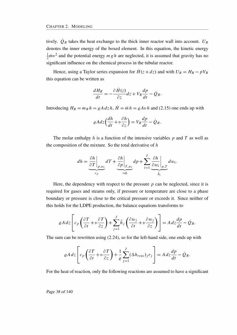
CHAPTER 2. MODELING

tively. Q R takes the heat exchange to the thick inner reactor wall into account. UR

denotes the inner energy of the boxed element. In this equation, the kinetic energy12mv2 and the potential energy m g h are neglected, it is assumed that gravity has nosignificant influence on the chemical process in the tubular reactor.

Hence, using a Taylor series expansion for H(z + dz) and with UR = HR − pVR

this equation can be written as

d HR

dt= −

∂ H(z)∂z

dz + VRdpdt

− Q R.

Introducing HR = m R h = %A dz h, H = m h = %Av h and (2.15) one ends up with

%Adz(dh

dt+v

∂h∂z

)= VR

dpdt

− Q R.

The molar enthalpy h is a function of the intensive variables p and T as well asthe composition of the mixture. So the total derivative of h

dh =∂h∂T

∣∣∣∣p,wi︸︷︷︸

cp

dT +∂h∂p

∣∣∣∣T,wi︸︷︷︸

≈0

dp +

I∑i=1

∂h∂wi

∣∣∣∣p,T︸︷︷︸

hi

dwi .

Here, the dependency with respect to the pressure p can be neglected, since it isrequired for gases and steams only, if pressure or temperature are close to a phaseboundary or pressure is close to the critical pressure or exceeds it. Since neither ofthis holds for the LDPE production, the balance equations transforms to

%A dz

cp

(∂T∂t

+v∂T∂z

)+

J∑j=1

h j

(∂w j

∂t+v

∂w j

∂z

)= A dzdpdt

− Q R.

The sum can be rewritten using (2.24), so for the left-hand side, one ends up with

%A dz

cp

(∂T∂t

+v∂T∂z

)+

1%

J∑j=1

(1hreac) jr j

= A dzdpdt

− Q R.

For the heat of reaction, only the following reactions are assumed to have a significant

Page 38 of 140


influence,

• initiation (see reaction scheme (2.1) and (2.4)),

• propagation (see (2.5)) and

• termination (see (2.6) and (2.7))

Moreover, the heat of reaction is assumed to be the same for these reactions, in otherwords (1hini t

reac) ≡ (1h propreac ) ≡ (1hterm

reac ). Additionally, the pressure dynamics is veryfast, so one can safely suppose that a quasi-stationary approach for the pressure dy-namic holds.

Q R comprises the heat transfer caused by convection and the thermal transferthrough a thin laminar layer. Both effects are combined in the inner heat transferresistor kinner . Hence

Q R = kinner (T − T ∗)dz.

Here, depending on the inclusion of the energy balance for the reactor wall, T ∗ de-notes either the average temperature of the inner reactor wall TW or the coolant tem-perature TC . Moreover, the overall heat transfer coefficient kinner is

• either to be taken from Eq. (2.43) (if the additional energy balance equation forthe wall is included into the dynamic model), or

• defined by the following equation, if the large capacitance of the inner reactorwall is neglected for the transient behavior,

kinner =1

Ri + Rll,i + Rst,i + Rsl,i + RC,i(2.48)

with

Rst,i =r2 − r1

λst,i. (2.49)

Page 39 of 140

CHAPTER 2. MODELING

Finally, one ends up with

%cp

(∂T∂t

+v∂T∂z

)=

1%

J∑j=1

(1hreac) jr j −kinner

A(T − T ∗) (2.50)

I C : T (z,0) = T0(z) (2.51)

BC : T (0, t) = Tin(t) (2.52)

Note again, that depending on the application, kinner is defined by either (2.43) withT ∗

= TW or by (2.48) with T ∗= TC . Moreover, all parameters depend on temperature

and pressure, some are also dependent on the composition of the reactor mixture.

Coolant. For the coolant some simplifying assumptions hold as well. Again, it isassumed to have plug flow without any radial temperature distribution. The kineticand potential energy can be neglected. Additionally, pressure and mass flux are keptconstant and no reaction takes place. It is important to note that the flux directionis counter-current wise. Hence the energy balance equation for the dashed box inFig. 2.8(b) reads

%CcpC

(∂TC

∂t−vC

∂TC

∂z

)=

kouter

AC(T∗ − TC)−

kamb

AC(TC − Tamb) (2.53)

I C : TC(z,0) = TC,0(z) (2.54)

BC : TC(L , t) = TC,in(t) (2.55)

Here, kouter and kamb are the overall heat transfer coefficients accounting for the heattransfer to reactor or wall and to the ambience. Depending on the inclusion of theenergy balance equation for the inner reactor wall, kouter is either defined by Eq. (2.45)with T∗ = TW or by kouter = kinner with kinner from Eq. (2.48) and with T∗ = T .The heat transfer coefficient to the ambience kamb can be evaluated by the followingexpression

kamb =1

RC,o + Rsl,o + Rst,o + Rair + Riso + Ramb. (2.56)

The overall heat transfer coefficient kamb hence includes the following effects

Page 40 of 140


• heat transfer by convection (RC,o from coolant to outside and Ramb from insu-lation to outside)

• heat transfer by conduction (Rsl,o through the outer slime layer, Rst,o throughthe outer wall, Rair through the air gap and Riso through the insulation)

• heat transfer by radiation (in particular, Es , which is one summand in of Ramb)

The resistances are calculated by

RC,o =1

αC,oUoαC,o =

λC NuC

2(r3 − r2 −2ssl)

UC,o = 2π(r3 − ssl)

Rsl,o =ssl

λslUm,slUm,sl =

2πssl

ln r3r3−ssl

Rst,o =sst,o

λst,oUm,st,oUm,st,o =

2π(r4 − r3)

ln r4r3

Rair =sair

λairUm,airUm,air =

2π(r4 + sair − r4)

ln r4+sairr4

Riso =siso

λisoUm,isoUm,iso =

2π(r5 − (r4 + sair ))

ln r5r4+sair

Ramb =1

αairUamb + Esαair =

λair Nuair

2r5

Uamb = 2πr5

Es = 2π r5 εσT 4

iso − T 4amb

Tiso − Tamb.

The overall heat transfer coefficient Ramb includes both free convection and radia-tion. For the free convection, Nuair = Nu(Grair , Prair ). The Grashof number iscalculated using Grair = 8

(%airηair

)2 βairg r3

5 (Tiso − Tamb). In all equations Tiso = 50◦C .The Prandtl number is evaluated by Prair =

ηair cP,airλair

. The Nusselt number is com-puted using Eq. (25) in Sec. Gb7 of VDI-Wärmeatlas (1991). The heat transfer byradiation is calculated using the Stefan-Boltzman constant σ = 5.6704 10−8 W

m2 K 4 andthe emissivity ε = 0.93, i.e. it is assumed, that emissivity does not depend on thewavelength.

Page 41 of 140

CHAPTER 2. MODELING

2.2.2.5 Moment Equations

Generally speaking, moments are widely used in the modelling of polymerization sys-tems where chain length, branching or double bonds play an important role. Mainlythey are utilized in order to reduce the size of those models, since it is not necessary tobalance every single molecule. Using moments enables one to specify characteristicproperties of e.g. the chain length distribution, such as average chain length or widthof the distribution. But usually the information on the distribution itself is lost andcan only be recalculated using infinitely many moments.

Strictly speaking, if we think of wP,i , wR,i and wR,sec,i in terms of distributionsof dead, living and living secondary polymer with discrete chain length i , then

µPr = E(wr

P) =

∞∑i=1

irwP,i

is called the r -th moment of the chain length distribution (in the equation above: thedead polymer distribution) about zero. The zeroth moment is equivalent the averageweight fraction, the first moment can be seen as number average molecular weight,and the third moment the skewness or asymmetry of the distribution.

Using these moments, it is easy to compute the average chain length or widthof the distribution. The average chain length (or degree of polymerization) can beevaluated by

Pn =µP

1

µP0

,

i.e. the mean of the probability distribution about zero over its sum. The polydisper-sity (or width of the distribution) is calculated by

PD =

µP2

µP1

Pn=

µP0 µP

2

(µP1 )2

. (2.57)

In general the following equation holds for all moment balance equations (k =

Page 42 of 140


[P; R; R,sec]):

d(m Rµkr )

dt=

∞∑i=1

ir d(m Rwki )

dt= −ARdz

(%v

∂µkr

∂z+µk

r∂(%v)

∂z

)+µk

r,reac (2.58)

with

µkr,reac =

∞∑i=1

ir mki,reac = mk

1,reac +

∞∑i=2

ir mki,reac. (2.59)

Living Polymer (Primary) In order to determine the summands of (2.59), thefollowing two parts are used, one for a single molecule and one for the remain-der (2 . . .∞). For the single molecule, one can derive from the reaction scheme(Eqns. (2.1)–(2.13))

i = 1 : MR,1 AR dz

(2kthc3

M +

3∑ν=1

kp,Iν cMcRIν + kp,X cR X cM − kpcMcR,1

+ ktr,McM

∞∑j=1

cR, j − ktr,McMcR,1 − ktr,X cX cR,1

− kt,ccR,1

∞∑j=1

cR, j − kt,dcR,1

∞∑j=1

cR, j − kbbcR,1 + kbbcR,1

−ktr,PcR,1

∞∑j=1

j cP, j + kβ

∞∑j=2

cR, j,sec

j −1

,

and analogous, the second part reads

i ≥ 2 : MR,i AR dz(

kpcMcR,i−1 − kpcMcR,i + kp,seccMcR,i−1,sec

− ktr,McMcR,i − ktr,X cX cR,i

− kt,ccR,i

∞∑j=1

cR, j − kt,dcR,i

∞∑j=1

cR, j − kbbcR,i + kbbcR,i

Page 43 of 140

CHAPTER 2. MODELING

−ktr,PcR,i

∞∑j=1

j cP, j + kβ

∞∑j=i+1

cR, j,sec

j −1

.

Inserting both parts in (2.59) and finally in (2.58) yields for the zeroth of the threemoments of the living polymer distribution:

∂µR0

∂t+v

∂µR0

∂z=

%

MM

[2kth

%

MMw3

M +

3∑ν=1

kp,IνMM

MRIνwMwRIν − ktr,PµR

0 µP1

−(kt,c + kt,d

)(µR

0 )2+ kβ

MM

%wR,sec + kp,secwMwR,sec

+ kp,XMM

MR XwMwR X − ktr,X

MM

MXwXµR

0

](2.60)

I C : µR0 (z,0) = µR

0,0(z) (2.61)

BC : µR0 (0, t) = µR

0,in(t) (2.62)

Note that the following assumption is used in the derivation of that equation:MR,i = MM . Naturally, one would expect something like MR,i = i MM . But if this isassumed, most of the infinite sums could not be calculated by inserting the appropriatemoments. Hence the model could not be simplified since one would have to computeinfinite sums numerically.

The first and second moment equation are computed similarly and their modelequation is listed in the Appendix B. Note that for the derivation of those equations,the relations on finite and infinite summations listed in Appendix A are used.

Living Polymer (Secondary) As previously mentioned, secondary living polymeris an indication for the long-chain branching in the polymer. Hence it has a highimpact on the physical properties of the product. To derive the model equations forit, the general equation for the moment equations (2.58) is used. The reaction termµr,reac = µR,sec

r,reac of (2.58) is computed by

ARdz∞∑

i=1

MR,sec,i(iktr cRcP,i − kp,seccMcR,sec,i − kβcR,sec,i

).

Page 44 of 140


And with MR,sec,i ≡ MM this gives for the r -th moment

∂µR,secr

∂t+v

∂µR,secr

∂z=

%

MM

[ktr,PµR

0 µPr+1 −

(kp,secwM + kβ

MM

%

)µR,sec

r

](2.63)

I C : µR,secr (z,0) = µR,sec

r,0 (z) (2.64)

BC : µR,secr (0, t) = µR,sec

r,in (t) (2.65)

Note that the moment equations of both, the living primary (listed in detail in App. B)and the living secondary polymer do close, since the r -th living primary/secondarypolymer moment does not depend on its higher moments.

Dead Polymer The moments of the distribution of dead polymer are also calculatedby (2.58) using the following expression for the computation of µr,reac = µP

r,reac:

i = 1 MP,1 AR dz(

ktr,McMcR,1 + ktr,X cX cR,1 + ktdcRcR,1

+ ktr,PcR,1

∞∑j=1

j cP, j − ktr,PcRcP,1 + kβ

∞∑j=2

cR, j,sec

j −1

).

Higher indices lead to

i ≥ 2 MP,i AR dz(

ktr,McMcR,i + ktr,X cX cR,i + ktdcRcR,i

+12

ktc

i−1∑k=1

cR,kcR,i−k + ktr,PcR,i

∞∑j=1

j cP, j

− i ktr,PcRcP,i + kβ

∞∑j=i+1

cR, j,sec

j −1

).

Page 45 of 140

CHAPTER 2. MODELING

Inserting this in the general form of the moment equations (2.58) one obtains e.g. forthe first moment of the dead polymer distribution

∂µP1

∂t+v

∂µP1

∂z=

%

MM

[12

kβMM

%µR,sec

1 + ktr,P(µP

1 µR1 −µR

0 µP2)

+ ktr,MwMµR1 +

(ktc + ktd

)µR

0 µR1 + ktr,X

MM

MXwXµR

1

](2.66)

I C : µP1 (z,0) = µP

1,0(z) (2.67)

BC : µP1 (0, t) = µP

1,in(t) (2.68)

It is important to note that the higher (r ≥ 0) moment equations for the dead poly-mer do not close, i.e.

µr 6= f (µ0,µ1, . . . ,µr−1,µr ),

but the r -th moment depends on higher moments. To overcome that situation, a tech-nique introduced by Hulburt and Katz (1964) is used. They proposed an artificialclosure, which circumvents the problem above. Hence

µP3 =

µP2

µP1 µP

0(2 µP

0 µP2 −µP

1 ) (2.69)

2.2.3 Discretization

Since the model equations for the peripheral units (see Section 2.3) are represented bysystems of differential and algebraic equations, the flowsheet simulator DIVA is usedfor the numerical solution of the equation system. Hence the partial differential andalgebraic equations of the tubular reactor model have to be transformed into a systemof differential and algebraic equations. For this transformation an adaptive method oflines approach with a finite differences scheme is used. First order backward differ-ences are taken for first order derivatives, for second order derivatives a second ordercentral scheme is chosen. The adaptation can be done statically or dynamically.

In a static adaptation scheme, for some time integration steps, the grid is fixed.Then in an additional regridding step a new grid point distribution is calculated, where

Page 46 of 140


grid points may be inserted or dropped. This recalculated grid point distribution iskept fixed for the successive time integration steps until a new regridding is required.Hence the number of grid points might change during simulations, whereas it remainsconstant if a dynamic adaptation mechanism is used. For the second approach noadditional regridding step is required, the grid moves continuously during the timeintegration. The dimension of the system is increased by the additional partial dif-ferential equation for the grid movement. Hence the overall system increases by thenumber of grid points. The flowsheet simulator DIVA requires a fixed number of statesduring the simulation run, hence, for the discretization of the partial differential andalgebraic equation system the dynamical adaptation scheme has to be used.

The discretization with a Method of Line approach utilizes a variable grid with Nz

grid nodes0 = z1 < z2(t) < . . . < zNz−1(t) < zNz = L ,

i.e., the first and the last grid node are fixed to the boundaries. The position of the gridnodes are continuous functions and have to be introduced as additional state variables,that add to the number of system state variables.

For the considered adaptive Method of Lines approach, the position of the gridnodes follows the equidistribution principle introduced by Dorfi and Drury (1987).They suggested an adaptive grid which has regions of high resolution where necessary.This allows larger steps for the time integration. For this purpose, the model equationsare transformed to the new moving grid according to

∂x j

∂t

∣∣∣∣zn(t)

=dx j,n

dt−

∂ x j

∂zdzdt

∣∣∣∣zn(t)

. (2.70)

This formulation represents the Lagrangian of the time derivative of any state x j inthe tubular reactor at a grid node zn(t). At the boundaries, z1(t) and zNz(t) the gridnodes are fixed and

∂x j

∂t

∣∣∣∣zν(t)

=dx j,ν

dtν = 1, Nz. (2.71)

Additional equations are required to determine the positions of the inner grid points.

Page 47 of 140

CHAPTER 2. MODELING

The general form of these equations reads

τE(x,z,κ)dzdt

= g(x,z,κ), (2.72)

where τ and κ are temporal or spatial regularization parameters and z ∈ IRNz is a vec-tor containing the inner grid points. Grid smoothing (spatial or temporal) is necessaryin order to avoid numerical problems caused e.g. by an overlapping of grid point tra-jectories or by oscillations of the grid point movement. Both, matrix E ∈ IRNz×Nz andthe function vector g ∈ IRNz are based on the spatial equidistribution principle, wherea monitor function M(x) for the estimation of the discretization error is used and thegrid nodes are placed such that this error is small. In this work, an arc-length monitorfunction is used,

M(z,x) =

√√√√1+LJ

J∑j=1

(1x j

∂ x j

∂z

)2

. (2.73)

It is also possible to use higher order derivatives in the monitor function. Taking thesecond derivative e.g. monitors not the gradient but the curvature of the graph of thestate variables. This results in

M(z,x) =

√√√√√1+L2

J

J∑j=1

(1x2

j

∂2x j

∂z2

)2

.

Therein, x j is used to make each of the summands dimensionless. Moreover,the value of x j should be chosen such that all summands contribute with a similarmagnitude to the monitor function. L denotes the length of the reactor. Of coursenot all states have to be included into that function, in fact, including all states justenlarges the number of entries into the Jacobian (we would have a sub-matrix with adense structure) and hence increases the computation time and storage requirement.

In an ideal grid node arrangement the discretization error is distributed uniformlyacross the spatial coordinate. The equidistribution principle postulates that integralsover adjacent sub-domains of a monitor function have to be equal, i.e. are constant

Page 48 of 140


over the whole domain. Hence∫ zn

zn−1

M(z,x)dz =

∫ zn+1

zn

M(z,x)dz ∀ n ∈ [2, Nz −1]. (2.74)

A discrete form of Eq. (2.74) is

ζn−1

Mn−1=

ζn

Mn∀ n ∈ [2, Nz −1] (2.75)

with the discrete form of the monitor function,

Mn =

√√√√1+LJ

J∑j=1

(1x j

x j (zn+1)− x j (zn)

zn+1 − zn

)2

(2.76)

and with the grid point concentration ζ ∈ IRNz−1

ζn =1

zn+1 − zn. (2.77)

Since Eq. (2.75) is algebraic, it is not yet of the form that is proposed in (2.72)(see Dorfi and Drury (1987)). To avoid an overlapping of grid points, the spatialmovement of the grid nodes is controlled. Introducing the spatial smoothing parame-ter κ > 0 the grid point concentration ζn is replaced by their numerically anti-diffusedcounterpart ζn ,

ζ1 = ζ1 −κ(κ +1)(ζ2 − ζ1) (2.78a)

ζn = ζn −κ(κ +1)(ζn − ζn−1) n ∈ [2, Nz −1] (2.78b)

ζNz = ζNz −κ(κ +1)(ζNz−1 − ζNz). (2.78c)

Then one can substitute (2.75) using the Eqns. (2.78)

ζn−1

Mn−1=

ζn

Mn∀ n ∈ [2, Nz −1]. (2.79)

The spatial smoothing parameter κ influences the ratio of adjacent grid points and

Page 49 of 140

CHAPTER 2. MODELING

gives a simple handle to avoid overlapping or a high concentration of grid nodeslocally. Verwer et al. (1989) have shown, that if κ satisfies the following condition

κ

κ +1≤

ζn

ζn−1≤

κ +1κ

,

then a non-smooth grid point distribution is impossible. In particular, κ � 1 almostfixes the grid points to their initial position, whereas 0 < κ ≤ 1 allows an aggressiveplacement of the grid nodes.

Still, the introduction of ζn yields no differential equation. So, besides spatialsmoothing, also temporal smoothing is used to avoid numerical problems. Therefore,the algebraic equations (2.79) are transformed into ordinary differential equations in-troducing the smoothing parameter τ ,

ζn−1 + τ d ζn−1dt

Mn−1=

ζn + τ d ζndt

Mn. (2.80)

Substituting (2.78) into (2.80) and using

dζn

dt= ζ 2

n

(dzn+1

dt−

dzn

dt

), (2.81)

it is straightforward to derive the matrix E in the following form (cf. Eq. (2.72))

e1,1 0 0 0 0 0 0 · · · 0

e2,1 e2,2 e2,3 e2,4 0 0 0 · · · 0

e3,1 e3,2 e3,3 e3,4 e3,5 0 0 · · · 0

0. . .

. . .. . .

. . .. . . 0 · · · 0

... · · · en,n−2 en,n−1 en,n en,n+1 en,n+2 · · ·...

0 · · · 0. . .

. . .. . .

. . .. . . 0

0 · · · 0 0 eNz−2,Nz−4 eNz−2,Nz−3 eNz−2,Nz−2 eNz−2,Nz−1 eNz−2,Nz

0 · · · 0 0 0 eNz−1,Nz−3 eNz−1,Nz−2 eNz−1,Nz−1 eNz−1,Nz

0 · · · 0 0 0 0 0 0 eNz ,Nz

︸︷︷︸

:=E

The elements of E are listed in detail in App. C (Eqns. (C.1)). Moreover, the elementsof the right hand side vector g of (2.72) are specified there (Eq. (C.2)).

Page 50 of 140


In order to reduce the error prone work of discretizing all equations manually,the tool SyPProT (Köhler (2002)) has been used to transform the system of partialdifferential equations into a system of differential and algebraic equations, as thisis required for the simulator DIVA. For the initiator weight fractions, the method isapplied in detail in the next section.

2.2.3.1 Example

Here, the partial differential equations for the initiators (according to Eq. (2.24)) areused to illustrate the application of the moving grid scheme. In particular, Eq. (2.24)applied to the initiators Iν,ν = 1,2,3 yields

∂wIν (z, t)∂t

+v(z, t)∂wIν (z, t)

∂z= −kIν (z, t)wIν (z, t). (2.82)

Discretizing this equation with a fixed, equidistant grid, using first order backwarddifferences, one ends up with

wIν (0, t) = wIν (z1, t) = wIin (2.83)dwIν (zn, t)

dt+v(zn, t)

wIν (zn, t)−wIν (zn−1, t)zn − zn−1

= −kIν (zn, t)wIν (zn, t)

∀ n ∈ [2, Nz], (2.84)

or, (2.84) rewritten in the semi-implicit notation DIVA requires

dwIν (zn, t)dt

= −v(zn, t)wIν (zn, t)−wIν (zn−1, t)

zn − zn−1− kIν (zn, t)wIν (zn, t). (2.85)

Alternatively, Eq. (2.82) can be discretized using an adaptive grid following theequidistribution principle. Then the partial differential equations for the initiatorsyield in semi-implicit discretized form

dwIν (zn, t)dt

−wIν (zn, t)−wIν (zn−1, t)

zn(t)− zn−1(t)dzn(t)

dt

=−v(zn, t)wIν (zn, t)−wIν (zn−1, t)

zn(t)− zn−1(t)− kIν (zn, t)wIν (zn, t) ∀ n ∈ [2, Nz].

(2.86)

Page 51 of 140

CHAPTER 2. MODELING

Note that in this equation, the grid position zn(t) is not a constant but a state variable.

The monitor function in the LDPE model is only a function of one state vari-able, namely the zeroth living polymer moment, µR

0 (z, t). Hence the discrete monitorfunction is

Mn =

√√√√1+ L

(1

µR0

µR0 (zn, t)−µR

0 (zn−1, t)zn(t)− zn−1(t)

)2

. (2.87)

Note that increasing the number of monitored state variables, does not increase themodel size itself. Instead, this influences the number of Jacobian elements and hencealso leads to a higher memory consumption.

Moreover, the values of the spatial and temporal smoothing parameters κ and τ

is chosen with 2.0 and 0.1 respectively. So the distance between adjacent grid pointsmay vary in an interval of [2

3;32 ].

2.2.4 Validation

In the next two sections, the validation of the tubular reactor as the main process unitin the LDPE production plant is shown. The reference profile is the result of thesteady state simulator Luposim T, developed by the BASF company for Basell. Forsimplicity, at first, the coolant flux direction is co-current wise, since in Luposim T,the counter current coolant flux is approximated iteratively using a shooting method.

At first, only one module is used for the comparison between the two simulationtools. After that, using the model for the whole tubular reactor, the influence of thediscretization is discussed.

2.2.4.1 Validation of one Module

For the validation of one module, a high resolution fixed grid with 1000 grid nodes iscompared to data given by the cooperation partner. Those results have been obtainedusing the steady state simulator Luposim T. According to the cooperation partner,these results show very good agreement with measured real plant data. Hence theirsteady state simulator results serve here as reference data for model validation. Forthat validation data of only one module with a coolant flux that is operated co-currentwise is used. In Fig. 2.9 on top the temperature profile in the reactor is plotted on the

Page 52 of 140


z/L [−]

Θ [−

]

0 0.02 0.04 0.060.7

0.75

0.8

0.85

0.9

0.95

1

ref. data (Luposim T)DIVA

z/L [−]

ΘC

[−]

0 0.02 0.04 0.060.76

0.765

0.77

0.775

0.78

z/L [−]

wM

/wr [−

]

0 0.02 0.04 0.061.7

1.75

1.8

1.85

1.9

1.95

2

z/L [−]

wP/w

r [−]

0 0.02 0.04 0.060

0.05

0.1

0.15

0.2

0.25

z/L [−]

MF

I [−

]

0 0.02 0.04 0.060.2

0.4

0.6

0.8

1

1.2

1.4

Figure 2.9: Temperature profiles, the mass fractions of monomer and polymer andthe melt flow index at steady state conditions

left. On the right the coolant temperature is depicted. Please note, that the tempera-ture profiles in the top row of the diagram are made dimensionless using the referencetemperature Tre f . Hence 2 =

TTre f

and 2C =TC

Tre f. In the bottom row on the left the

mass fraction of monomer and in the middle the one of polymer can be seen. Again,the values are divided by a “reference weight fraction” wr . Moreover, the bottomright graph shows one physical property of the polymer, the melt flow index. The val-ues obtained by Luposim T are indicated by red circles, simulation results of DIVA isdrawn with a solid blue line. It has to be pointed out, that the simulator tools solvingthe equations in either DIVA or Luposim T are completely different from each other.The flowsheet simulator DIVA solves the whole set of system equations simultane-ously for each time integration step, whereas the steady state simulator Luposim T

integrates along the spatial coordinate, and hence only has to solve approx. 30 ODEs

Page 53 of 140

CHAPTER 2. MODELING

at the same time. Despite of the difference in numerical solution methods the resultsmatch very precisely in steady state.

The important quantities for the product are not only melt flow index, but also themoments of the chain length distributions. They are depicted in Fig. 2.10. In the leftcolumn the moments of the dead polymer chain length distribution are shown. Themiddle column depicts the moments of the living primary, the left one the moments ofthe living secondary polymer chain length distribution. Again, the simulation resultsobtained with DIVA match the industrial data precisely. The graph of the dead polymeralways has a positive gradient, since in neither of the reactions (2.1)–(2.13) polymer isconsumed. In contrast to that, the graphs of the living primary and secondary polymermoments have distinct local minima and maxima. This can be explained by the dif-ferent initiator types that are used. The profiles of their weight fractions are depicted

z/L [−]

µ 0P [−

]

0 0.02 0.04 0.060

0.5

1

1.5

2x 10

−4

z/L [−]

µ 0R [−

]

0 0.02 0.04 0.060

0.5

1

1.5

2x 10

−7

z/L [−]

µ 0Rse

c [−

]

0 0.02 0.04 0.060

2

4

6

8x 10

−10

z/L [−]

µ 1P [−

]

0 0.02 0.04 0.060

0.05

0.1

0.15

0.2

z/L [−]

µ 1R [−

]

0 0.02 0.04 0.060

2

4

6x 10

−4

z/L [−]

µ 1Rse

c [−

]

0 0.02 0.04 0.060

1

2

3x 10

−6

z/L [−]

µ 2P [−

]

0 0.02 0.04 0.060

200

400

600

800

z/L [−]

µ 2R [−

]

0 0.02 0.04 0.060

2

4

6ref. dataDIVA

z/L [−]

µ 2Rse

c [−

]

0 0.02 0.04 0.060

0.01

0.02

0.03

Figure 2.10: Zeroth, first and second moments of the chain length distributions.

Page 54 of 140


z/L [−]

wI1

[−]

0 0.02 0.04 0.060

0.5

1

1.5x 10

−5

z/L [−]

wR

I1 [−

]

0 0.02 0.04 0.060

1

2

3

4x 10

−11

z/L [−]

wI2

[−]

0 0.02 0.04 0.060

2

4

6x 10

−5

z/L [−]

wR

I2 [−

]0 0.02 0.04 0.06

0

2

4x 10

−10

z/L [−]

wI3

[−]

0 0.02 0.04 0.060

2

4

6x 10

−5

z/L [−]

wR

I3 [−

]

0 0.02 0.04 0.060

2

4x 10

−10

ref. data (Luposim T)DIVA

Figure 2.11: The weight fractions of initiator and their radicals.

in the left column of Fig. 2.11, the right column shows their radicals. The initia-tor three instantaneously decomposes into radicals, resulting in the first “propagationwave” and the first maximum in the zeroth moments of living radicals. The radicalsare rapidly consumed along the reactor and since the growth reaction is exothermic,also initiator two and one start building radicals. The decomposition rate of those rad-icals is higher than the termination rate of dead polymer, hence the second maximumin the zeroth moment evolves. Then no reaction (except thermal initiation) providesnew radicals, hence the moment of living polymer decreases to zero.

It has been shown, that the rigorous dynamical model (without an energy balancefor the reactor wall) is able to reproduce precisely the reference values of the steadystate simulator Luposim T. The number of grid points used for this comparison is

Page 55 of 140

CHAPTER 2. MODELING

Θ [−

]

z/L [−]0 0.01 0.02 0.03 0.04 0.05 0.06

0.7

0.75

0.8

0.85

0.9

0.95

1

wM

/wr [−

]

z/L [−]0 0.02 0.04 0.06

1.7

1.75

1.8

1.85

1.9

1.95

2

wP/w

r [−]

z/L [−]0 0.02 0.04 0.06

0

0.05

0.1

0.15

0.2

0.25

1000 fixed 100 fixed 60 fixed 60 adaptive

Figure 2.12: Temperature profiles and the mass fractions of monomer and polymer atsteady state conditions using different discretization schemes and grid

points

unrealistic high. A model of the tubular reactor, with its 29 partial differential andalgebraic equations for each of the 16 modules would result in a system of 464 ·

103 ordinary differential and algebraic equations. Such a system is far too large forstandard computers systems available right now. So, in a next step, the influence ofthe selected discretization method on the simulation result of one module is discussed.

2.2.4.2 Influence of Discretization

The previous section proves the validity of the detailed model for one module. Here,the influence of the discretization will be discussed in detail. In order to select the bestdiscretization method for the purpose of this work, the fully featured rigorous model

Page 56 of 140


is used for this comparison, i.e. the energy balance equation for the wall is included.Moreover, the coolant is operated counter-current wise. For this configuration nosimulation data from Luposim T is available, hence the detailed dynamical modelwith a high resolution fixed grid serves as reference.

The following configurations are compared to each other,

• high resolution fixed grid (1000 grid nodes),

• intermediate resolution fixed grid (100 grid nodes),

• low resolution fixed grid (60 grid nodes) and

• low resolution adaptive grid (60 grid nodes).

In Fig. 2.12, process variables, such as dimensionless temperature 2 and weightfractions of monomer wM and LDPE wP are depicted along the spatial coordinate.Both, wM and wP are made dimensionless using a reference weight fraction wr .Again, only one module i.e. one cooling jacket, is considered here. The referenceprofile, which is the result of the simulation using the high resolution fixed grid isdrawn in all three graphs with a solid blue line. The dash-dotted red line representsthe intermediate resolution grid, the dotted red line the low resolution fixed and thedashed black line the low resolution adaptive grid. As one can observe, the numberof grid points of either fixed or moving grid does not influence the profile of thoseprocess variables significantly. Only in regions of the tubular reactor where largertemperature gradients occur, some slight deviations between the four discretizationschemes are visible.

But for such issues as optimization or control, also product properties play animportant role. These properties can be expressed in terms of the number average,

Pn =µP

1

µP0

(2.88)

variance

σ 2=

µP0 µP

2 − (µP1 )2

(µP0 )2

(2.89)

Page 57 of 140

CHAPTER 2. MODELING

and skewness

γ =µP

3σ 2 . (2.90)

They are depicted in the left column of Fig. 2.13. Number average means here an aver-age chain length, variance is the averaged squared deviation from the arithmetic mean.The standard deviation is defined as the square root of the variance. Both standard de-viation and variance describe the spread of a distribution, as does the polydispersitydefined in (2.57). To describe, whether a distribution is asymmetric, the skewnesscan be used. If the distribution is normal, then the skewness calculated with central-ized moments is zero, if the right tail is longer than the left one, then the skewnessis negative, otherwise it will be positive. In Fig. 2.13 right column shows the sec-ond moments of the living primary and secondary and the dead polymer chain-lengthdistribution. Again, the solid line represents the grid with 1000 fixed grid points, thedash-dotted line the fixed grid with 60 nodes and the dashed line the adaptive gridwith the same number of grid nodes.

From this picture it is obvious, that there exist significant differences between thehigh and the low resolution grids in general. But if one compares these differencesin magnitude, the adaptive low resolution grid performs considerably better than thefixed one. E.g. the error in the variance of the distribution is approx. 25% usingthe fixed grid, whereas with the adaptive grid it is 10% less. The reason for theselarge deviations in the properties of the distributions can be seen in the right columnof Fig. 2.13. Even though the zeroth moment of the living polymer chain lengthdistribution is used in the monitor function M(z,x) (Eq. (2.73)), the number of fixedgrid points is too small to resolve the formation of living polymer precisely. Hencethese deviations sum up in higher moments of living polymer and naturally the erroris transferred to the moments of the dead polymer chain length distribution.

In Tab. 2.1 the simulation times with the different discretization schemes are com-pared. The fastest calculation time, utilizing a low-resolution fixed equidistant grid ischosen as the reference time (tdisc,re f = 42.42 s on a standard PC equipped with anAMD Athlon™ 64 Processor 3500+ and 1G B RAM). In order to make the results ofthis comparison transferable to other computer systems, not the absolute values of thesimulation time but multiples of the fastest solution are shown. In the upper row, the

Page 58 of 140


Pn [−

]

z/L [−]0 0.02 0.04 0.06

400

600

800

1000

σ2 [−]

z/L [−]0 0.02 0.04 0.06

0

500

1000

γ [−

]

z/L [−]0 0.02 0.04 0.06

0

5000

10000

15000

µ 2P [−

]

z/L [−]0 0.02 0.04 0.06

0

500

1000

µ 2R [−

]z/L [−]

0 0.02 0.04 0.060

2

4

6

81000 fixed 100 fixed 60 fixed 60 adaptive

µ 2R,s

ec [−

]

z/L [−]0 0.02 0.04 0.06

0

0.01

0.02

0.03

0.04

Figure 2.13: Temperature profiles and the mass fractions of monomer and polymer atsteady state conditions using different discretization schemes and grid

points

results for the validation of one module are tabulated (see Sec. 2.2.4.1). There, themodel without energy balance for the wall has been used and that the coolant is as-sumed to flow co-current wise. It is interesting to see, that the fixed grid with 100 gridnodes and the low-resolution grid both have similar simulation times, even though the

Wall energy Coolant flux Fixed Adaptivebalance direction 1000 100 60 60

– co-current 83.3 1.9 1.0 2.04 counter-current 110.7 4.0 1.8 12.6

Table 2.1: Comparison of simulation times tdisctdisc,re f

on a standard with an AMDAthlon™ 64 Processor 3500+ and 1G B RAM.

Page 59 of 140

CHAPTER 2. MODELING

number of state variables is lower by a factor of 1.6. Moreover, the high-resolutionscheme, which is larger in size by a factor of 16.7, takes 83.3 times longer to be solved.In general, the effort of solving equation systems numerically increases exponentiallywith system size. Additionally, also the type of equations and back-mixing effectsincrease simulation times. This can be seen in the bottom row of the table, whichtabulates the results of a simulation with the energy balance equation for the wall andwith the counter-current flow. Both effects contribute to an almost doubled simulationtime for the fixed low-resolution grid. The fixed intermediate-resolution grid scaleswith the same factor, but the adaptive grid now takes three times as long as the fixedgrid with the same error. Even though, the simulation is much faster, it is not possibleto use the fixed grid with 100 grid nodes, since this adds up to 29 · 16 · 100 = 46000equations, which has not been possible to solve on a standard PC. Here, the adaptive

0 0.02 0.04 0.060

0.005

0.01

0.015

0.02

0.025

0.03

0.035

0.04

0.045

0.05

z/L [−]

τ [−

]

0.76 0.78 0.80.2

0.3

0.4

0.5

0.6

0.7

0.8

0.9

z/L [−]

τ [−

]

Figure 2.14: Movement of grid nodes during the startup of the tubular reactor

Page 60 of 140

2.3. PERIPHERAL UNITS

grid is smaller by a factor of 1.6 (30 ·16 ·60 = 28800).

To see how the grid node distribution evolves with simulation time, Fig. 2.14displays the movement of the grid nodes of two modules during the startup of thetubular reactor. The abscissa displays the dimensionless axial coordinate, the y-axisthe simulation time τ =

tsimtres

. This is a dimensionless number accounting for the realsimulation time tsim and the residence time of the reactor tres . One grey line representsthe position of a grid node. The left figure shows the grid node distribution right afterthe initiator injection in the first module, the right one shows the arrival of a wave atthe fourth section, in particular, at the thirteenth module. In both figures it can be seenthat the grid node concentration moves rapidly to the left boundary of the plot andafter only a few milli-τ the steady-state is established. It is important to see, that inthe left figure, the grid nodes are not exclusively locked to the left picture boundary,there is also a higher concentration at z/L ≈ 0.02, which is due to the fact, that thezeroth living polymer moment is used for the monitor function. And from Fig. 2.10follows directly, that there a higher resolution is required.

Disregarding the longer simulation times, the low-resolution adaptive grid offersboth reasonable model size (which has been important because of memory constraintsof standard PCs at that time) and sufficient accuracy. So, this discretization method isused throughout the remainder of this work.

2.3 Peripheral Units

The periphery of the tubular reactor can be summarized in a few single units. First ofall the mixing units, then the compressors, the separators and some heat exchangers.Ideal controllers are assumed, that keep the controlled variables at the desired setpoint, e.g. temperatures in the separators, where the model equations and underlyingassumptions are given in Section 2.3.3.

2.3.1 Mixer

In the plant there are several units for mixing different streams, e.g. mixing freshethylene with the recycle from the low pressure separator, or the injection of new ini-tiator into the reactor tube. All of these units have in common that they are assumed

Page 61 of 140

CHAPTER 2. MODELING

not to have storage capacities. Thus, the different fluxes mix instantaneously, mean-ing that the mixer is modeled as a continuous stirred tank reactor with infinitely smallvolume. Hence these systems can be described by algebraic equations solely. There-fore all mixers in the plant are described by algebraic mass, component and energybalances.

0 = mmix −

J∑j=1

min, j , (2.91)

0 = mmixwmix,i −

J∑j=1

min,i, jwin,i, j ∀ i = 1, . . . , I −1. (2.92)

It is assumed, that the heat capacity of modifier is the same as the one of ethene.Moreover, the heat capacity of the monomer is assumed to be constant in those mixers,hence

0 = Tmix mmix −

J∑j=1

min, j Tin, j . (2.93)

2.3.2 Compressor

There are three compressors in the plant, a so-called ’booster’, which compresses theethylene gas from the low pressure recycle to the feed pressure of the freshly addedmonomer/modifier mixture. The feed is followed by a pre-compressor, which bringsthis gas stream to an intermediate pressure. Afterwards, the hyper-compressor, whichcompresses the monomer/modifier mixture up to the operating pressure of approx.3000 bar . The booster consists of two successive stages, the pre-compressor consistsof three stages, the final pressure is reached after another two stages in the hyper-compressor.

A rating model of compressors in general correlates the behavior of real gases tothe behavior of ideal gases. The change of state of ideal gases can be described bythe polytropic exponent, which the The American Society of Mechanical Engineers

Page 62 of 140


(1997) define in their test code as

n =

log(

pout

pin

)log

(V in

V (pout ,Hout )

) , (2.94)

where pin and pout are inlet and outlet pressure and V is the volumetric flow rateat inlet and real outlet conditions pout and Tout . However, for such a descriptionit is necessary to use performance map curves. These curves correlate machine effi-ciency and machine head to volumetric flow rate and either inlet guide vane or angularspeed, depending on whether the machine is angle or speed controlled. Since both,performance map curves for the efficiency and for the head of all compressors are notspecified by the cooperation partner, it is assumed that temperature and pressure arecontrolled ideally. Then, in general, the k-th stage of a compressor consists of thefollowing equations

0 = min,k +γ min,rec − mout,k

%i,k VRk ,idwi,k

dt= min,kwin,i,k +γ min,recwin,i,rec − mout,kwi,k, i = 1, . . . , NC −1

0 =

NC∑i=1

wi,k −1.0

with

γ =

1 for k = 1

0 else.

Moreover, min,k+1 = mout,k . Note that in these compressor units only two compo-nents are present, namely ethylene and modi f ier . Both are either freshly fed to theprocess or come from the recycle lines. Moreover, it is supposed that the physicalproperties of both modifier and ethylene are identical. Since both, pressure and tem-perature are controlled ideally, they are assumed to be constant at a given set point,i.e. Tk = const. and pk = const..

Page 63 of 140

CHAPTER 2. MODELING

2.3.3 Separator

The separators are required to split up the mixture of monomer, modifier and poly-mer. It is assumed that monomer and modifier are removed ideally from the mixture,meaning that only polymer leaves the plant.

In the plant, there are two separating units, one where the mixture at high pres-sure is relaxed to an intermediate pressure and a succeeding one, where relaxationto a moderate pressure, slightly higher than ambience pressure takes place. The twodifferent pressure levels are introduced to save compression energy from the low tothe intermediate pressure level.

High pressure separator To fully describe the high pressure flash unit, mass bal-ance, component mass balance and energy balance equations are required. The globalmass balance is assumed to be quasi-stationary, so are the component mass balancesfor the three components (monomer, modifier and polymer) and the energy balance.Moreover, the liquid phase contains all three components, where the gaseous phase(which is recycled in subsequent recycle lines) does not contain any product. Using anreasonable fast controller, the flash will be both isothermal and isobaric. To describethe vapor-liquid-equilibrium a generic equation (which was fitted to given measureddata) is used

wliq,M = wliq,M(p f lash,T f lash).

Hence the model reads

0 = min,hp − mvap − mliq

0 = min,hpwin,hp,X − mvapwvap,X

0 =

NC∑i=1

wvap,i −1.0

0 =

NC∑i=1

wliq,i −1.0

0 = wvap,P

0 = wliq,X

Page 64 of 140


0 = min,hphin,hp − mvap(hvap +1hvap,M)− mliqhliq .

Note that from the energy balance equation not the temperature is calculated (remem-ber that isothermal behavior was assumed), but the mass flux of the vapor phase.Moreover, it is assumed that polymer and modifier are separated ideally, i.e. no poly-mer but all modifier is recirculated in the high pressure recycle (wvap,P = wliq,X = 0).

Low pressure separator The low pressure flash is modelled to separate ideally thepolymer P from the unreacted monomer M , hence only polymer is withdrawn fromthe plant and all monomer is recycled. So the model equations for this unit read

0 = min,lp − mM − m P

0 = win,lp,Mmin,lp − mM .

Additionally, the flash is temperature controlled, so that Tlp = const..

2.3.4 Recycles

The recycle lines of Fig. 2.1 are assumed to be lag systems and the heat exchangerscan be used to control the temperature at arbitrary set points. So the volume of therecycles is modeled by simple tank units.

0 = min − mrec (2.95)

%rec,M Vrecdwrec,M

dt= minwin,M − mrecwrec,M (2.96)

0 = wrec,X +wrec,M −1.0 (2.97)

0 = Trec − Tset . (2.98)

Note, that in the high pressure recycle line, the only components are monomer M andmodifier X . The low pressure recycle consists of pure ethene, so there the componentmass balance and the closure are not required to describe the unit model.

Page 65 of 140

CHAPTER 2. MODELING

2.4 Simple Model of the Plant

The simplified model only includes the essential process characteristics and is there-fore only suitable for a qualitative but not a quantitative prediction of the processbehavior.

Due to it’s simplicity it is well suited for a numerical bifurcation analysis usingthe methods and tools described in Mangold et al. (2000a). The influence of the mostimportant process parameters is studied systematically. These are: the feed flow rate,the feed concentration of monomer and the heat exchange.

Initiator Initiator Initiator Initiator

Cooling jacket Cooling jacketCooling jacket Cooling jacket

Separator

Ethylene Polyethylene

Reaction Separation

Figure 2.15: Flowsheet representation of the simple mathematical model

Fig. 2.15 shows the flowsheet of the simplified plant for the production of lowdensity polyethylene using a tubular reactor. The simplified tubular reactor is 1000 m

long and has a inner diameter of 4 cm. Fresh monomer is fed to the plant and mixedwith the recycle from the separator. The free radical polymerization of LDPE is car-ried out in the tubular reactor. Therefore initiators are added to the monomer streamat the inlet of the tubular reactor. The reaction starts, the temperature rises, initiatordecompose into radicals, radicals bind monomer and hence monomer gets consumed,whereas polymer is produced. The reaction heat is removed using four different cool-ing jackets. Here, the length of each of the four cooling zones is identical. A coolingzone is located in between two injectors.

At the outlet, unreacted ethylene is separated from the polymer in one flash unit,

Page 66 of 140

2.4. SIMPLE MODEL OF THE PLANT

the polymer is withdrawn from the plant, whereas the monomer is recycled to thesystem.

For comparison, the flowsheet of the real production plant is depicted in Fig. 2.1.Next, the main differences in the plant structure are listed in detail.

As one can observe, compressors are neglected completely. Additionally, the pres-sure in the tubular reactor is assumed to be constant (p = 3000 bar ). This implies,that the simple model does not need two recycle lines. Recall, that in the real produc-tion process the only reason for having two recycle lines are savings in compressionenergy. Hence, the recycle lines are operated at that pressure to which the flash unitexpands the ingoing monomer/polymer mixture. Since the pressure drop in the reac-tor is neglected, the simple model only has one flash unit and only one recycle line.This has no effect on the total recycle flow rate.

The next difference which is obvious just by comparing Fig. 2.15 to Fig. 2.1, isthe number of coolant jackets. In the real production process, there are in total 16different coolant cycles which can be operated co- or counter current wise. For thesimplified process the number of jackets is decreased to four. Moreover, the simplemodel assumes a constant coolant temperature, which of course saves an additionalpartial differential equation.

Additionally, the initiator mixture consisting of three different initiators, whichdecompose at different temperature levels, is substituted by a single initiator, resolvingat intermediate temperature levels.

2.4.1 Reaction Scheme

The reaction scheme used for the simplified model of the tubular reaction differs sig-nificantly from the very detailed scheme in the rigorous dynamic model. Here onlythe main reactions, characteristic for all polymerization reactions are taken into ac-count. Side reactions are completely neglected. Hence only the following reactionsare considered,

IνkIν

−−−→ 2 RIν initiator decomposition, (2.99)

RIν + Mkp,Iν


Page 67 of 140

CHAPTER 2. MODELING

Ri + Mkp

−−−→ Ri+1 propagation, (2.101)

Ri + R jkt,c

−−−→ Pi+ j termination by combination and (2.102)

Ri + R jkt,d

−−−→ Pi + Pj termination by disproportion. (2.103)

Buback (1980) reported that the rate of thermal initiation of ethylene is much lowercompared to the other initiation reactions, so that reaction is neglected. There aretwo more differences when comparing the reaction scheme (2.99)-(2.103) to the moredetailed one (2.1)–(2.7), the number of components is reduced by six, since only oneinitiator equation is required and the modifier is neglected. Even though two differentinitiators (Iν for ν = 1,2) are used (decomposing at low and intermediate tempera-tures), one component mass balance equation is sufficient, since initiator decompos-ing at low temperatures is injected only at the inlet of the tubular reactor, the secondinitiator is added at all successive injection pumps. All initiator is consumed in thesection where it is injected. Moreover, the additional counter for the occurrence ofdouble bonds is not included in the termination reaction (2.103).

2.4.2 Model Equations

2.4.2.1 Tubular Reactor

Both in the rigorous and in the simpler dynamical model of the tubular reactor in theLDPE production process, it is supposed that the following assumptions hold

• one homogeneous liquid phase and

• plug flow.

In order to reduce both complexity and model size more simplifications have to betaken into account, such as

• a constant pressure drop over the reactor length

• reduction of the number of coolant jackets down to four, that are additionallyoperated at a constant temperature level

• a constant average heat transfer coefficient

Page 68 of 140


• reduction of the number of initiators to two

• a constant temperature and a negligible time delay in the recycles

• a negligible energy balance equations for coolant and inner reactor wall

So there are seven components in the reactor, two initiators, their radicals, monomerand living and dead polymer. Adding the energy balance for the reactor temperature,the models compare in their size as tabulated in Tab. 2.2.

For the simple model, only data available from literature is be used. There, theparameters are usually published based on concentrations rather than on weight frac-tions. Hence the simple model equations are formulated in terms of concentrationsand the component mass balances for the species are

• initiator concentrations

∂cIν

∂t+v

∂cIν

∂z= −kIν cIν ∀ ν = 1,2, (2.104)

• initiator radicals concentrations

∂cRν

∂t+v

∂cRν

∂z= 2kIν cIν − kp,Iν cRν cM ∀ ν = 1,2, (2.105)

• monomer concentration

∂cM

∂t+v

∂cM

∂z= −

2∑ν=1

kp,Iν cRν cM − kp cMλR0 , (2.106)

Detailed model Simplified modelNumber of modules 16 4Number of PDAEs per module 30 7Grid resolution 60 50Total number of DAEs ≈ 30000 ≈ 1000

Table 2.2: Comparison of model sizes of the tubular reactor – rigorous versus simpli-fied model

Page 69 of 140

CHAPTER 2. MODELING

• overall concentration of living polymer

∂λR0

∂t+v

∂λR0

∂z=

2∑ν=1

kp,Iν cRν cM −(ktc + ktd

)(λR

0 )2, (2.107)

• overall concentration of dead polymer (product)

∂λP0

∂t+v

∂λP0

∂z=(0.5ktc + ktd

)(λR

0 )2. (2.108)

Knowing that the energy balance for the wall is neglected and that the coolanttemperature TC is constant, it is straightforward to derive the energy balance

%cp(∂T

∂t+v

∂T∂z

)= 1h

(kpcMλP

0 +(1

2ktc + ktd

)(λP

0 )2

+

2∑ν=1

kIν cIν

)−

Uπr2 (T − TC). (2.109)

In the equations above, c j denotes the concentration of species j . These statevariables are distributed over the domain. v is the flow rate of the reaction mixture,which is a concentrated variable. Both, % = 540 kg

m3 and cp = 2.7 k JkgK are constant over

the length of the reactor. So are the heat of reaction 1h = 95 k Jmol and the heat transfer

coefficient U = 80 WmK .

For all state variables x = [ci λj0 T ]T , the following initial and boundary con-

ditions hold

I C : x(z, t = t0) = x0(z) (2.110)

BC : x(z = 0, t) = xin(t) (2.111)

The reaction rates and their parameters are given in Tab. 2.3. The values for theinitiator decomposition have been reported by Kim and Iedema (2004) and the valuesfor all propagation and termination reactions are taken from Lee and Marano (1979).

Page 70 of 140


initiator decomposition kI1 = 1.35 ·1013 exp(

−117476−0.2805·10−5 pIRT

) [1s

]kI2 = 2.89 ·1014 exp

(−138237−1.012·10−5 p

IRT

) [1s

]propagation kp = 5.88 ·104 exp

(−29704+2.325·10−5 p

IRT

) [m3

gmol s

]initiation kp,I1 = kp,I2 = kp

termination by combination ktc = 1.075 ·106 exp(

−1247+1.422·10−5 pIRT

) [m3

gmol s

]by disproportion ktd = ktc

Table 2.3: Kinetic rate expressions used in the simple model

2.4.2.2 Peripheral Units – Simple Model

For the description of the rigorous dynamic mathematical model of the low-densitypolyethylene production plant, additional units for compression, separation and heatexchange are used. Though these units do not contribute significantly to the size of themodel, most of the units are neglected or simplified. In particular, the two differentflash units of the detailed model operated at different pressure levels for recovery ofcompression energy, are concatenated into a single flash unit. Additionally, this flashunit ideally separates product from unreacted monomer, which makes it unnecessaryto include a equilibrium correlation into that model,

0 = nin − nrec − nL D P E (2.112)

0 = ninxM,in − nrecxM,rec (2.113)

0 = ninx Iν ,in − nrecx Iν ,rec (2.114)

0 = ninxR,in − nrecxR,rec (2.115)

0 = Trec − T f i x . (2.116)

Since only one recycle line is used for the simple model, the compressors can beneglected as well. Hence, only a mixing unit is required, which ideally mixes theincoming feed and the recycled material from the flash unit. The model equations for

Page 71 of 140

CHAPTER 2. MODELING

this unit read

0 =nrec

M+ VF − VR (2.117)

0 = nrecxM,rec + VF cM,F − VRcM (2.118)

0 = nrecx Iν ,rec + VF cIν ,F − VRcIν (2.119)

0 = nrecxR,rec + VF cR,F − VRcR (2.120)

0 = TR − T f i x . (2.121)

Note that in (2.117) a volume balance occurs, however, in this mixing unit no reactiontakes place which changes the mole number, hence a general mass balance may alsobe stated in terms of volume.

So far for both, the rigorous and the simpler model, the mathematical model equa-tions have been derived. The next chapter shows simulation results for both steadystate and dynamical solution of the LDPE production line.

Page 72 of 140

Chapter 3

Simulation Results

It does not matter how slowly you go, so long as you do not stop.

– Confucius

In this chapter, simulation results of both, the detailed and the simple model willbe presented. At first, in Sec. 3.1, results of the rigorous model are compared tothe reference, which is the solution of a simulation run of the steady state simulatorLuposim T. For the steady state comparison, the system without an additional energybalance for the thick reactor wall is used, since Luposim T does not account for thiseffect. Then dynamic simulation results with the detailed mathematical model areshown in Sec. 3.2. These include simulations of only the tubular reactor during startupoperations or disturbances, as well as disturbances in input variables of the wholeproduction process from the given nominal operating point. Finally, in Sec. 3.3, thedetailed model is compared to a simpler one. Since the agreement between simpleand rigorous model is very good, the nonlinear analysis of the process is carried outusing the simpler and hence smaller model.

3.1 Steady State Simulation Results – Rigorous Model

First, the focus is on the validation of the rigorous model of the tubular reactor. As ithas been already shown in Sec. 2.2.3, the results of the rigorous dynamic model of onemodule match perfectly the results of the steady state simulator Luposim T, inspite ofthe different solution strategy and the large difference in the number of equations of

73

CHAPTER 3. SIMULATION RESULTS

z/L [−]

Θ [−

]

0 0.1 0.2 0.3 0.4 0.5 0.6 0.7 0.8 0.9 10.7

0.8

0.9

1

Luposim TDIVA

z/L [−]

ΘC

[−]

0 0.1 0.2 0.3 0.4 0.5 0.6 0.7 0.8 0.9 10.7

0.72

0.74

0.76

0.78

z/L [−]

wM

/wr [−

]

0 0.2 0.4 0.6 0.8 11.2

1.4

1.6

1.8

2

z/L [−]

wP/w

r [−]

0 0.2 0.4 0.6 0.8 10

0.2

0.4

0.6

0.8

Figure 3.1: Comparison of steady state simulation results from Luposim T and DIVA– temperatures, monomer and polymer weight fractions

the systems, that are solved numerically. DIVA on the one hand side is an equationbased simulator that solves DAE systems simultaneously in each integration step.The steady state simulator Luposim T on the other side integrates along the spatialcoordinate and implements the counter-current coolant flow via a shooting method.Clearly, the numerical effort for Luposim T is much smaller compared to the state-of-the-art simulator DIVA, but of course its commitment is different. Whereas Luposim T

only solves the steady state equations, DIVA additionally solves dynamic systems andcan be used for dynamic and steady state optimizations and for nonlinear analysis.These results will be presented in Sec. 3.3.

Page 74 of 140

3.1. STEADY STATE SIMULATION RESULTS – RIGOROUS MODEL

3.1.1 System Without Energy Balance for the Wall

In this section, the steady state simulation results of Luposim T are compared to theresults of DIVA. Note that Luposim T only simulates the tubular reactor, hence onlysimulation results of this unit are considered. Moreover, coolant is operated counter-current wise. Remember that Luposim T approximates a counter-current coolant oper-ation using a shooting method. Looking at Fig. 3.1 it is obvious that the results of bothsimulators show very good agreement. Only at the end of the tubular reactor, thereare some larger deviations in the coolant temperature. In particular at z/L = 0.75, theinlet temperature of the coolant is the same, but the outlet temperature of this cool-ing zone at z/L ≈ 0.69 differs quite significantly. This is due to the fact, that DIVA

requires all variables to be elements in C1, unless implicit event functions are defined

z/L [−]

Nu

[−]

0 0.1 0.2 0.3 0.4 0.5 0.6 0.7 0.8 0.9 10

1000

2000

3000

4000

5000Luposim TDIVA

z/L [−]

Nu

[−]

0.5 0.55 0.6 0.65 0.7 0.75 0.8 0.85 0.9 0.95 10

100

200

300

400

Figure 3.2: Comparison of steady state simulation results from Luposim T and DIVA– Nusselt number in the tubular reactor.

Page 75 of 140


for these variables (C1 is the set of functions that are continuous and have a continu-ous first derivative). Since all variables in the tubular reactor are spatially distributed,that would imply numerous distributed event functions. Each event causes a localiterative search for the exact point in time, at which that event occurs. Therefore, sim-ulation times would exceed an acceptable limit, so such a procedure is not practicalfor a distributed parameter system. To avoid this, the discontinuous correlations havebeen converted into functions in C1. Both, the effect of such a transformation (whichis applied to the Reynolds number) and the effect of slight deviations at a transitionpoint can be seen in Fig. 3.2. There, the Nusselt number (Nu = f (Re, Pr)) is plottedagainst the length of the reactor. In the top figure, the whole reactor and in the bot-tom figure only the relevant sector is graphed. Again, the red and blue line representsimulation results of Luposim T and DIVA. To a large extent, there is good agreementbetween the two profiles. Only in the region with large deviations in coolant tempera-ture, a significant difference is visible. This can be explained first by small deviationsin the Reynolds number of the rigorous model, since this implies an earlier transitionfrom the turbulent to the turbulent-laminar domain. Moreover, the implementationof this transformation to a C1 function changes the limit points of the transient re-gion from turbulent to laminar Reynolds numbers. The region of transition becomesslightly larger, leading to the effect depicted in Fig. 3.2.

Another point which is very interesting from Fig. 3.2 in general, is the strongdependency of the Nusselt number on the location within the reactor. The Nusseltnumber decays from almost 4000 (for turbulent flows) down to 20, where the flow islaminar. Since Nu directly influences the heat transfer resistor Ri as one summandin the overall heat transfer coefficient from reactor to coolant (Eq. (2.43) or (2.48)),it is obvious, that the profile of the coolant temperature has almost no gradient withrespect to reactor length in section four (c.f. Fig. 3.1).

Apart from that difference, and despite of the fact, that only the adaptive low-resolution discretization scheme is used, the profiles in Fig. 3.1 match very well.Nevertheless, in Sec. 2.2.4.2 it has been shown, that even though there are only mi-nor deviations in process variables such as temperature or weight fractions, in someproperties of the distribution there may well occur larger deviations. Hence, Fig 3.3shows these properties, such as number average Pn , variance or skewness. More-over, the melt flow index is shown in the bottom right graph. As one can observe,

Page 76 of 140


z/L [−]

Pn [−

]

0 0.2 0.4 0.6 0.8 1550

600

650

700

750

800

850

z/L [−]

σ2 [−]

0 0.2 0.4 0.6 0.8 10

500

1000

1500

2000

z/L [−]

γ [−

]

0 0.2 0.4 0.6 0.8 12000

4000

6000

8000

10000

12000

14000

16000

Luposim TDIVA

z/L [−]

MF

I [−

]

0 0.2 0.4 0.6 0.8 10.2

0.4

0.6

0.8

1

Figure 3.3: Comparison of steady state simulation results from Luposim T and DIVA– properties of the dead polymer distribution and the melt flow index.

the deviations in the product (z/L = 1) are only in a range of 3 − 6%. But duringthe polymerization, the properties of the distribution such as variance and most of allskewness show larger deviations up to 30%. This error is introduced by the discretiza-tion. Recall, that for a high-resolution scheme, the moments calculated by DIVA andLuposim T match accurately, whereas for lower resolutions, in all moments of theradical distribution and hence also of the dead polymer distribution a discretizationerror becomes visible. In general, due to the discretization, DIVA “produces” longerchains in the beginning. The influence of this effect becomes smaller, the longer thereaction takes place. Hence, at the outlet, both simulation results agree quite well andusing the low-resolution adaptive discretization scheme does not introduce deviationsin the product with are unacceptable. In the sequel, the adaptive Method of Lines isused for all simulations using the rigorous dynamic model for the tubular reactor.

Page 77 of 140


z/L [−]

Θ [−

]

0 0.1 0.2 0.3 0.4 0.5 0.6 0.7 0.8 0.9 10.7

0.8

0.9

1

without wallwith wall

z/L [−]

ΘC

[−]

0 0.1 0.2 0.3 0.4 0.5 0.6 0.7 0.8 0.9 10.7

0.72

0.74

0.76

0.78

z/L [−]

wM

/wr [−

]

0 0.2 0.4 0.6 0.8 11.2

1.4

1.6

1.8

2

z/L [−]

wP/w

r [−]

0 0.2 0.4 0.6 0.8 10

0.2

0.4

0.6

0.8

Figure 3.4: Comparison of steady state simulation results neglecting the energy bal-ance for the wall and including it – temperatures and weight fractions of

monomer and polymer.

3.1.2 System With Energy Balance for the Wall

In this section, the energy balance for the reactor wall is included into the mathemat-ical description of the tubular reactor. First the influence of the wall in steady stateis discussed. In Fig 3.4 the steady state profiles of dimensionless temperatures andnormalized weight fractions are depicted. The red lines represent the model without,the blue lines the model with additional partial differential equation for the wall. Onecan see from the top graph in Fig. 3.4 that the reactor temperature in the first sectionand in the last section is significantly influenced by the reactor wall equation, eventhough the heat transfer coefficient of the wall is included into the model without theadditional equation. These deviations are due to the fact that the model with wall

Page 78 of 140


energy balance allows heat transport also in axial direction, which causes peaks andminima to smooth out. This is most obvious in the first and last section of the tubularreactor. In the first section the highly exothermic reaction starts and the coolant isused to lower the reactor temperature. Since in the second section the reaction is re-ignited by adding new initiator, again temperature rises. But in the case with energybalance for the reactor wall, the wall allows heat transport in axial direction. Hencethe temperature before and after the injector is higher. This effect additionally causesthe initiator injected at z/L = 0.25 to decompose faster, producing more heat of re-action. So even though the energy balance for the wall should chop off peaks, themaximum temperature in sections two and three are higher.

z/L [−]

wI1

[−]

0 0.2 0.4 0.6 0.8 10

0.5

1

1.5x 10−5

z/L [−]

wI2

[−]

0 0.2 0.4 0.6 0.8 10

2

4

6x 10−5

z/L [−]

wI3

[−]

0 0.2 0.4 0.6 0.8 10

2

4

6x 10−5

z/L [−]

wR

I1 [−

]

0 0.2 0.4 0.6 0.8 10

1

2

3

4x 10−11

z/L [−]

wR

I2 [−

]

0 0.2 0.4 0.6 0.8 10

0.5

1

1.5

2x 10−10

z/L [−]

wR

I3 [−

]

0 0.2 0.4 0.6 0.8 10

2

4x 10−10


Figure 3.5: Comparison of steady state simulation results neglecting the energy bal-ance for the wall and including it – weight fractions of initiator and their

radicals

Page 79 of 140


Looking only on the steady state results, it cannot yet be decided, whether anenergy balance for the wall is required to describe the main features of the productionprocess of low-density polyethylene. However, since the inner wall adds an enormousthermal capacity to the system, the transient behavior should be more affected by theaddition of the wall balance. Therefore, in the next section, dynamic simulations withboth models are performed.

Θ(z

/L=1

) [−]

τ [−]0 1 2 3 4 5 6

0.75

0.8

0.85

0.9


wM

/wr(z

/L=1

) [−]

τ [−]0 2 4 6

1.3

1.4

1.5

1.6

1.7

1.8

1.9

2

wP/w

r(z/L

=1) [

−]

τ [−]0 2 4 6

0

0.1

0.2

0.3

0.4

0.5

0.6

Figure 3.6: Comparison of dynamic simulation results neglecting the energy bal-ance for the wall and including it – temperature and weight fractions of

monomer and polymer

Page 80 of 140

3.2. DYNAMIC SIMULATION RESULTS – RIGOROUS MODEL

3.2 Dynamic Simulation Results – Rigorous Model

In this section, at first, the two dynamic rigorous models with and without energybalance equation are compared to each other in their transient behavior. In the begin-ning, only the tubular reactor will be considered, then in Sec. 3.2.2 the recycles areclosed and the dynamic behavior of the uncontrolled LDPE production plant will beinvestigated.

3.2.1 System Without Recycle

Here, two cases are discussed, the startup of the tubular reactor when there are nomaterial recycles, and the transient behavior when disturbances are applied to theinlet of the reactor. For both models, the adaptive Method of Lines approach is usedfor the discretization of the PDAE system.

3.2.1.1 Startup

At first, a comparison in the transient behavior of the startup of the uncontrolled tubu-lar reactor with and without energy balance for the wall is shown. From the steadystate behavior, it is obvious that there exists almost no difference, hence for simplicity,that equation might be dropped. Fig 3.6 depicts process variables such as dimension-less temperature or normalized weight fractions at the outlet of the tubular reactor.The red line represents the model without an additional energy balance for the wall,the blue line represents the model which includes that equation. Of course, the resultis not very surprising, indeed the transient behavior is affected. In the beginning of thesimulation, both models act very similar, in fact in 2 only slight differences becomevisible for the first few τ time units. But after τ = 1, in the model where the heatcapacity is neglected, the steady state is reached. However, the model with energybalance needs approx. 6τ until the steady state establishes. Hence, even though theinfluence of the reactor wall on the steady state is of minor importance (see Fig. 3.4),it is not admissible to neglect it for the transient behavior.

So, for the simulation of a startup of the tubular reactor, the model which accountsfor the heat conduction in the wall is used. Fig. 3.7 shows the dynamic profiles for thestartup already graphed in Fig. 3.6. Except for the coolant, for the startup simulation

Page 81 of 140


z/L [−]

Θ [−

]

0 0.1 0.2 0.3 0.4 0.5 0.6 0.7 0.8 0.9 10.7

0.8

0.9

1

z/L [−]

ΘC

[−]

0 0.2 0.4 0.6 0.8 1

0.72

0.74

0.76

z/L [−]

ΘW

[−]

0 0.2 0.4 0.6 0.8 1

0.75

0.8

0.85

z/L [−]

wM

/wr [−

]

0 0.2 0.4 0.6 0.8 11.2

1.4

1.6

1.8

2

z/L [−]

wP/w

r [−]

0 0.2 0.4 0.6 0.8 10

0.2

0.4

0.6

0.8

Figure 3.7: Profiles of process variables during startup operation, plotted over thereactor length

it is assumed, that the initial values of the distributed parameters are already at feedcondition. Hence the initial profile, indicated by the black solid line, is constant.Moreover this implies, that in the reactor no initiator, no radicals and no polymerexists. Since the coolant is operated at different levels, for the coolant only the inlet isat steady state conditions, whereas the initial values of the distributed state variablesare set to an arbitrary but reasonable temperature. Then for τ > 0, initiator is addedat all four injectors. Since initiator decomposing at a low temperature level is onlyadded at the inlet of the tubular reactor, there the reaction starts. The reaction ishighly exothermic and so the temperature rises and one front propagates through thereactor. At the same time, at the second injection valve initiator is added but veryfew is consumed, hence the reaction is in an extinguished state. As soon as the front

Page 82 of 140


from the first injector passes by the second one, also there the reaction starts, becauseof the higher temperature level. The accumulation of unconsumed initiator and thearrival of the reaction front at the third injector causes temporarily a high temperaturepeak after the addition of initiator. But as initiator gets consumed, the sharp peak issmoothened which prevents that product decomposition takes place. Then the frontleaves the reactor and after 6τ the steady state profile is established.

Since startup is time consuming, a case study is performed, that gives some insightto the potential of dynamic optimization. The following cases will be considered

• case 1: the case, which has been introduced in the previous paragraph, all ini-tiators are added simultaneously at steady state flow rates,

• case 2: as case one, but additionally, for 1τ =14 , the third initiator resolving at

low temperatures is added in all injectors,

• case 3: as case two, the feed flow rate of the third initiator is doubled,

• case 4: as case three, the amount of the third initiator is doubled again,

• case 5: initiators are added sequentially after 1τ =14 , 1

2 and 34 at steady state

flow-rates,

• case 6: initiators are added sequentially after 1τ = 1, 74 , 9

4 and 52 at steady state

flow-rates.

Herein, the difference 1τ is always the absolution difference related to the startof the simulation, i.e. τ = 0. Hence for case five, initiator is always added when thereaction front reaches the injector. In case six, first a steady state has to be reached.Since this holds for the tubular reactor without any material recycles when the reactionfront leaves the reactor, one has to wait 1τ1 = 1 time units for the first wave, thenadditional 1τ2 =

34 time units (1τ = 1τ1 +1τ2) etc..

Fig. 3.8 shows the simulation results of this case study. The graphs show processvariables at the outlet of the tubular reactor. In the top row, the dimensionless tem-perature 2 =

TTre f

is shown in both the left and the right picture. The right plot is amagnification of the first 2τ time units. The bottom row graphs the melt flow index asone property of the product. Also here, the right diagram is a magnification of the first

Page 83 of 140


Θ(z

/L=1

) [−]

τ [−]0 2 4 6 8

0.7

0.75

0.8

0.85

0.9

0.95

1

case 1case 2case 3case 4case 5case 6

Θ(z

/L=1

) [−]

τ [−]0 0.5 1 1.5 2

0.7

0.75

0.8

0.85

0.9

0.95

1

MFI

(z/L

=1) [

−]

τ [−]0 2 4 6 8

0.2

0.4

0.6

0.8

1

MFI

(z/L

=1) [

−]

τ [−]0 0.5 1 1.5 2

0.2

0.4

0.6

0.8

1

Figure 3.8: Comparison of time constants for different startup strategies of the tubu-lar reactor

time units. The blue solid line represents case one which has already been used in thecomparison of the transient behavior with and without wall. The red color indicatesthat for these cases the initiator decomposing at a low temperature level is used in allinjectors and the black lines indicate that the initiators are added sequentially. Whatbecomes obvious is that of course case six takes longest to reach the steady state.Another interesting observation can be made from Fig. 3.8. Although the reactor tem-perature has not reached a steady state, product in terms of melt flow index is alreadywithin the specification limits after only 1.8 τ . Moreover, the different strategies donot significantly improve the startup of the tubular reactor, except for the fact, thatmethod six takes by far longest. But looking in more detail at the right column, onecan see, that the case studies marked in red color (all injection valves add the initiator

Page 84 of 140


0 2 4 6 8 10

0.9

1

1.1

Θ(z

/L=1

) [−]

τ [−]

−30% initiator+30% initiator

0 2 4 6 8 10

0.9

1

1.1

Θ(z

/L=1

) [−]

τ [−]

−10% monomer−30% monomer

0 2 4 6 8 10

0.9

1

1.1

Θ(z

/L=1

) [−]

τ [−]

−80% coolant+80% coolant

0 2 4 6 8 10

0.9

1

1.1

Θ(z

/L=1

) [−]

τ [−]

−5K TC

+5K TC

0 2 4 6 8 10

0.9

1

1.1

Θ(z

/L=1

) [−]

τ [−]

−15K TF

+15K TF

0 2 4 6 8 10

0.9

1

1.1

Θ(z

/L=1

) [−]

τ [−]

−10% modifier+10% modifier

Figure 3.9: Influence of disturbances on the outlet temperature – without recycles

resolving at low temperature for τ =14 ) are slightly ahead of the other strategies. And

among each other, the case study which adds most of the third initiator is performingbetter than the others. Hence, even by simple case studies, there is some improvementvisible, so there is potential for a dynamic optimization of the startup operation.

3.2.1.2 Disturbances

The influence of the disturbances on the transient behavior will be discussed utiliz-ing the rigorous mathematical model of the tubular reactor with energy balance forthe reactor wall. Characteristic disturbances to be considered were specified by thecooperation partner. In particular,

• step change in feed flow rate of monomer (−30%),

Page 85 of 140


0 2 4 6 8 100

1

2

3

4

MFI

(z/L

=1) [

−]

τ [−]


0 2 4 6 8 100

1

2

3

4

MFI

(z/L

=1) [

−]

τ [−]


0 2 4 6 8 100

1

2

3

4

MFI

(z/L

=1) [

−]

τ [−]


0 2 4 6 8 100

1

2

3

4

MFI

(z/L

=1) [

−]

τ [−]

−5K TC

+5K TC

0 2 4 6 8 100

1

2

3

4

MFI

(z/L

=1) [

−]

τ [−]

−15K TF

+15K TF

0 2 4 6 8 100

1

2

3

4

MFI

(z/L

=1) [

−]

τ [−]


Figure 3.10: Influence of disturbances on the melt flow index – without recycles

• step change in feed flow rate of coolant (±80%),

• step change in feed flow temperature (±5K ),

• step change in feed flow rate of modifier (±50%),

• step change in feed flow rate of initiators (±30%).

Results of this simulations are depicted in Fig. 3.9 and 3.10. There the black dot-ted line refers to a simulation without any disturbances. So the initial value for thesimulations indeed is a steady state. In all graphs, in general, the blue line denotes anegative, the red line a positive sign of the step change, except for the feed rate of themonomer (top diagram in the right column). This feed flow rate is only disturbed inthe direction towards smaller feeds, hence the blue line indicates the smaller, the red

Page 86 of 140


line the larger step change. From all diagrams in Fig. 3.9 it follows immediately, thatthe system is nonlinear, since step changes of the same size into different directionsdo not lead to a symmetric shape of the graphs (symmetric with respect to the steadystate value). Moreover, looking at the second row in Fig. 3.9, a higher cooling capac-ity (either caused by increase in the coolant flow rate or by a decrease of the coolanttemperature) results in higher outlet temperatures at the reactor end. This can be ex-plained using the Nusselt number of the reactor flow. Increasing the cooling capacitycauses the first temperature maximum to be shifted downstream. This means that atthe injector in the second section the reactor temperature is already at a higher initialvalue. Thereby in section two, the reaction is more intense and more monomer getsconverted. The same holds for the third section, so that the rector content becomesmore viscous and the transition to a laminar flow regime moves upstream. Recall thatlaminar flow always implies smaller Nusselt numbers and the overall heat transfer co-efficient becomes worse. So, a higher coolant capacity in section four has only littleinfluence on the outlet temperature, resulting in a rise of that temperature.

Fig. 3.10 shows the influence of the step changes on the melt flow index, onecharacteristic property of the produced low-density polyethylene. What is most strik-ing there, is that although the effect of e.g. step changes in initiator feed flow rateand coolant flow rate have a similar effect on the outlet temperature, the MFI is onlyslightly affected by that disturbance. But the modifier and the monomer feed flowrate show a significant impact on that physical property. However, this is an expectedresult, since in general modifiers are used to control the chain length distribution. Thechain length distribution has large impact on the physical properties and the melt flowindex is one way to measure the physical properties of the polymer. Hence, bothfeed flow rates (monomer and modifier) must have a large influence on the physicalproperties.

Generally speaking, the rigorous model for the uncontrolled system with no recy-cles proves to be robust, all given disturbances can be simulated, although the sim-ulation times tend to be considerably large. Depending on the kind of disturbance,simulation runs with a duration of more than 8h can occur.

The dominating time constant in the detailed dynamic model without recyclesis introduced by the inclusion of a “semi-distributed” energy balance equation forthe reactor wall. Hence the energy balance equation for the reactor wall cannot be

Page 87 of 140


z/L [−]

Θ [−

]

0 0.1 0.2 0.3 0.4 0.5 0.6 0.7 0.8 0.9 10.7

0.75

0.8

0.85

0.9

0.95

1

Θ(z

/L=1

) [−]

τ [−]0 2 4 6 8 10

0.9

0.91

0.92

0.93

0.94

0.95

0.96

Θ(z

/L=1

) [−]

τ [−]0 50 100 150

0.9

0.91

0.92

0.93

0.94

0.95

0.96

without recylceswith recycles

Figure 3.11: Influence of the recycles on the time constant of the tubular reactor

neglected.

3.2.2 System With Recycle

In the sequel, the recycle lines are closed, but still the reactor is operated uncontrolled,except for the assumptions that have been made in Chap. 2, e.g. compressor is alwayscapable to track any given inlet pressure. Main issue of this section is the investigationon how the recycles influence both the time constant and the stability of the system.Therefore step tests are performed. First the steady state profile of the model withrecycles and the profile of the model without recycles are compared. This comparisonand the simulation results of the same step change in the feed rate is done in Fig. 3.11.In the top of that figure, the temperature profile are graphed. In the first two sections,these profiles match very well, although in the last section there are larger deviations.

Page 88 of 140


0 20 40 60

0.9

1

1.1

Θ(z

/L=1

) [−]

τ [−]


0 20 40 60

0.9

1

1.1

Θ(z

/L=1

) [−]

τ [−]


0 20 40 60

0.9

1

1.1

Θ(z

/L=1

) [−]

τ [−]


0 20 40 60

0.9

1

1.1

Θ(z

/L=1

) [−]

τ [−]

−5K TC

+5K TC

0 20 40 60

0.9

1

1.1

Θ(z

/L=1

) [−]

τ [−]

−15K TF

+15K TF

0 20 40 60

0.9

1

1.1

Θ(z

/L=1

) [−]

τ [−]


Figure 3.12: Influence of disturbances on the outlet temperature – with recycles

As in Sec. 3.1.1, the reason for the larger deviations in section four of the tubularreactor can be found in the Nusselt number. Slight changes in Reynolds number leadto large changes in the Nusselt number and so the overall heat transfer coefficientbecomes worse. Then the coolant jackets are not able to remove the heat of reactionas efficiently as before. Nevertheless, feed into the tubular reactor is the same, henceit is assumed that the agreement of both models is well enough.

The influence of the recycles on the overall time constant is shown in the bottomrow of Fig. 3.11. There the simulation result of a small decrease in the feed flow rateof monomer on both systems is depicted. The right graph shows a magnification ofthe first 10τ time units, the left one displays the whole simulation time. Since steadystate profiles of the reactor temperature differ at the outlet of the tubular reactor, theinitial value of the dimensionless temperature 2 is different. In fact, 2(τ = 0) in

Page 89 of 140


the bottom row is equal to 2(z/L = 1) in the top row. From the two diagrams itfollows immediately, that the recycles increase the overall time constant of the low-density polyethylene production process by a factor of 10–15. For the considereddisturbance, the system without recycles reaches a new steady state after approx. 5τ

time units, whereas the system with recycles needs more than 50τ until the steadystate is reached. Hence, not the large heat capacity of the reactor wall, but the volumeof the recycle lines determines the largest time constant in the LDPE production plant.

3.2.2.1 Disturbances

Each of the disturbances that have been already introduced in Sec. 3.2.1.2 is now alsoimposed on the system with material recycles. In Fig. 3.12 and Fig. 3.13 the resultsare shown. In both figures, the scale of the ordinate is the same, but the scale ofthe abscissa is different. It has been shown in the previous section, that the materialrecycles considerably increase the dominating time constant in the system. So, inorder to reach a steady state, the simulation time has to be increased. In fact, thesimulation time is even larger than depicted in the graphs (τ = 150), but for a betteroverview, in the plots it is zoomed into 60τ . For all disturbances, except the largerdecrease in the monomer feed rate, a new steady state settles. Also the simulationwith the step change in the modifier feed rate reaches a new steady state, but the timeconstant is ≈ 100τ for that disturbance.

In the system with material recycle, the effect of a change in the coolant capacityis smaller compared to the system without recirculation. This behavior is caused bythe recycle lines. From Sec. 3.2.1.2 it has been concluded, that the outlet temperatureof the reactor is higher for an increase in the heat capacity of the coolant. This leadsto less conversion, and the mean of the chain length distribution Pn =

µP1

µP0

is lower. Alower mean results in higher densities, hence the overall heat transfer worsens and theoutlet temperature will be higher. On the other hand, less conversion means higherrecycle flow rates, which means that the reactor flow rate is also higher and hence thelaminar region with a small overall heat transfer coefficient will be shorter. So, thecoolant is able to withdraw more heat of reaction. Both effects compensate and so astep change in the coolant capacity shows less impact on the outlet temperature.

The most interesting effect of the recycles is the influence on the stability of the

Page 90 of 140


0 20 40 600

1

2

3

4

MFI

(z/L

=1) [

−]

τ [−]


0 20 40 600

1

2

3

4

MFI

(z/L

=1) [

−]

τ [−]


0 20 40 600

1

2

3

4

MFI

(z/L

=1) [

−]

τ [−]


0 20 40 600

1

2

3

4

MFI

(z/L

=1) [

−]

τ [−]

−5K TC

+5K TC

0 20 40 600

1

2

3

4

MFI

(z/L

=1) [

−]

τ [−]

−15K TF

+15K TF

0 20 40 600

1

2

3

4

MFI

(z/L

=1) [

−]

τ [−]


Figure 3.13: Influence of disturbances on the melt flow index – with recycles

overall system. This can be seen in the top right diagram in both Fig 3.12 and 3.13.The small step change in the monomer feed rate has no influence on the stability ofthe system, after approx. 10τ , a new steady state is obtained. But a large step inthe monomer feed rate renders the rigorous mathematical model of the LDPE pro-duction process unstable. The direct effect of the step change results in a higher endtemperature. The temperature rise is drastically from 2 = 0.93 to 2 ≈ 1. Since theoutlet temperature drops, initially it looks as if also for the large step a new steadystate could be attained. However, the high temperature also causes more monomerto be converted, hence the recycle flow rate is smaller and so the feed to the reactorbecomes less. Higher residence times also imply that the region of laminar Nusseltnumber increases. As a consequence, after τ ≈ 10, the temperature rises again, theheat of reaction cannot be removed by the coolant, the product decomposes. The ther-

Page 91 of 140


mal runaway behavior however cannot be observed in the controlled plant, hence thisphenomenon is a feature of this uncontrolled model implementation.

This observation though is the starting point for a thorough nonlinear analysis ofthe mathematical model of the LDPE production plant. For this purpose, the rigor-ous model turned out to be unmanageable. The size of the model, even though a lowresolution discretization scheme has already been selected, is too large for the appli-cation of the nonlinear analysis methods available in DIVA. Hence the simple modelof Sec. 2.4 has been derived.

3.3 Nonlinear Analysis – Simple Model

The nonlinear analysis in DIVA examines the behavior of the mathematical modelusing continuation methods. These methods calculate the steady state solution of asystem (1.1) as a function of one or two model parameters. Such a procedure is calleda parameter continuation. The continuation algorithm contains methods for the sta-bility analysis and for the detection of singularities. For the stability analysis in DIVA

there are two methods available, a k-step Arnoldi method (Sorensen, 1992) and a QRalgorithm of the LAPACK collection (DGEEV). The latter routine is a replacement ofthe EB07AD routine from the Harwell Library, as the developers of the Harwell Li-brary state that their routine is outdated. Hence, for the purpose of this work, boththe latest stable version of the Arnoldi algorithm (as a replacement for the previousbeta version) and the DGEEV routine have been implemented. One advantage of theArnoldi method is, that only the dominating eigenvalues are calculated, which reducescomputation times considerably for large systems. In fact, the Arnoldi method cal-culates approximations to a few eigenvalues with their corresponding eigenvectors.These approximations are called Ritz values or Ritz vectors respectively. However,these approximations sometimes give inaccurate results for the stability analysis ofthe steady states. So for this method it is recommended to validate the results of thestability analysis by dynamic simulations.

Nonlinear dynamics of reactor separator systems has received considerable inter-est during the last few years and various types and combinations of different reactionand separation processes were investigated. In particular, Pushpavanam and Kienle(2001) studied a first order exothermic reaction in a CSTR in combination with an

Page 92 of 140

3.3. NONLINEAR ANALYSIS – SIMPLE MODEL

isothermal, isobaric flash which is used for the recycle of unreacted reactant. In ad-dition, intermediate heat exchangers are used for energetic decoupling of the reactorand the separator unit. It was found that the behavior of such a system strongly de-pends on the flow control strategy. Most complicated patterns of behavior were foundfor a fixed feed flow to the reactor. In that case a total number of twenty-four differentbifurcation diagrams were predicted using singularity theory and it was shown thatthe behavior of such a reactor separator system is completely different from the standalone reactor investigated earlier in Uppal et al. (1974), for example.

In particular, it was found that at high Damköhler numbers,

Da =tprocess

treaction, (3.1)

two steady state solutions exist, which merge and disappear at a limit point if theDamköhler number is decreased. Hence, large operation regions were found with nosteady state at all. In these regions the recycle flow rate will increase continuously.In addition, isolated branches of steady state solutions (isolas) and Hopf bifurcationpoints were found. The latter are the origin of oscillatory behavior. Clearly, multi-plicity and instability of steady states is caused primarily by the exothermicity of thechemical reaction.

Recently, a similar system, a loop reactor for the polymerization of vinyl acetatewas investigated by Melo et al. (2003). They found that the transition from operationwithout material recycles to an operation with a partial recirculation of polymer so-lution is characterized by the evolution of oscillatory behavior. At low recycle ratesthey observed complex dynamics, including chaos. Moreover they predicted as manyas seven steady states for the reactor model. They identified the overall heat transfercoefficient as one of the key influence factors on the dynamic behavior.

Similar steady state solution curves with a single turning point were found for aplug flow reactor with a first order exothermic reaction by Kiss et al. (2003). As apractical application example, a LDPE reactor separator system was considered. Theplant configuration is very similar to the one considered here. It includes a tubularreactor with four different initiator feeds. This is equivalent to a system with fourdifferent tubular reactors in series leading to sequential bifurcations with multiplehysteresis. The analysis was based on a steady state model only and no prediction

Page 93 of 140


of dynamic behavior including stability was possible. Moreover, implications forpractically relevant operating conditions were not discussed.

This gap has been closed by Häfele et al. (2005). There, the simple model, derivedin Sec. 2.4 has been used for the nonlinear analysis of the model. In this work, theseresults will briefly be discussed.

3.3.1 Comparison – Rigorous Model and Simple Model

First the validity of the simple model should be checked using the steady state profileof the reactor temperature. Both profiles are shown in Fig. 3.14, the blue line indicatesthe rigorous model with energy balance equation for the wall, the red line representsthe solution of the simple model. Note that the initial conditions for both models, i.e.

z/L [−]

Θ [−

]

0 0.1 0.2 0.3 0.4 0.5 0.6 0.7 0.8 0.9 10.7

0.75

0.8

0.85

0.9

0.95

1

rigorous modelsimple model

Figure 3.14: Comparison of the steady state reactor temperature profile of the simpleand the rigorous model

Page 94 of 140


feed temperature and feed flow rate of monomer are approximately the same. In con-trast to the rigorous model, the simple model utilizes only two different initiators, onedecomposing at a moderate and one decomposing at a intermediate temperature level.Moreover, the first injection valve only adds initiator resolving at low temperatures.All other injectors add only the intermediate initiator, whereas in the rigorous model,always a mixture of at least two different initiators is used. From this difference, mostof the steady state deviations between the two models can be explained, such as sizeof peaks and gradient after an injector. But also the influence of a constant heat trans-fer coefficient is clearly visible in section four of the tubular reactor (z/L ≥ 0.75). Inthe rigorous model, the heat transfer is reduced by a factor > 10, whereas the simplemodel assumes constant heat transfer. Hence, as soon as a laminar flow establishes,the difference in the reactor temperature of the two models becomes larger. Corre-

τ’ [−]

Θ(z

/L ≈

0.2

⋅ 10

−3) [

−]

0 0.2 0.4 0.6 0.8 1 1.2 1.4 1.60.9

0.95

1

1.05

1.1

1.15

1.2

1.25

1.310 % decrease20 % decrease

Figure 3.15: Thermal runaway of the simple model

Page 95 of 140


lating the heat transfer coefficient to the polymer concentration would account for andecrease in the overall heat transfer in the simple model as well. Nevertheless, thoughquantitatively there are some deviations, the simple model is quantitatively a goodapproximation of the rigorous reference model.

This becomes even more obvious when looking at the responses on step changes inthe monomer feed concentration, which is depicted in Fig. 3.15. The abscissa showsthe dimensionless temperature 2( z

L = 0.2 ·10−3) =T (0.2·10−3)

Tre fover the dimensionless

time τ ′=

ttres,F

. Herein tres,F =VR

VM,Fwith the monomer feed rate VM,F . For this figure

both a smaller (−10%) and a larger (−20%) decrease in the fresh feed flow rate hasbeen applied to the uncontrolled simple model. Whereas for the small step change anew steady state is obtained, the temperature rises exponentially for the 20% decrease.This result matches the simulation results using the rigorous model with closed mate-rial recycles. In particular, the top right diagram of Fig. 3.12 also shows the thermalrunaway of the tubular reactor as a result of a large step change in the monomer feedflow rate. It should be noted, that even though both models predict the thermal run-away phenomenon, the location is different. The detailed model shows the runawayphenomenon at the end of the tubular reactor (z/L = 1), the simple model just afterthe first injector (z/L ≈ 0.2 · 10−3). Moreover, in practice, a proper control strategyprevents the occurrence of such phenomena in the plant. However, the phenomenonmight be explained by means of nonlinear analysis.

3.3.2 Bifurcation and Stability Analysis

Here, the bifurcation and stability analysis is applied to the simplified model of theLDPE tubular reactor production process. The variable that is selected for the param-eter continuation is the monomer feed flow rate, since this parameter seems to havemost effect on the stability of the overall system. The result of a parameter continu-ation is shown in Fig. 3.16. There, the blue solid line represents the stable solutions,the dashed red line indicates unstable solution branches. The normal operating pointis marked by the black circle filled with a grey pattern, where τ ′

= 1. The left diagramshows the dimensionless temperature, the right diagram the result of variations in τ ′

on the conversion in the plant. Note that for residence times less than 0.2, except ofthe trivial solution no other steady state solution exists. Trivial means that no reaction

Page 96 of 140


τ’ [−]

Θ [−

]

0 0.5 1 1.5 2

0.8

1

1.2

1.4

1.6

1.8

2

2.2

τ’ [−]

x M [−

]

Hopf bifurcation point

operating point

0 0.5 1 1.5 2

0

0.1

0.2

0.3

0.4

0.5

0.6

0.7

0.8

0.9

1stable unstable

Figure 3.16: Stability and bifurcation diagram

takes place, the reactor is extinguished, hence xM = 0.0, and 2 = 0.75. This is a goodagreement with the results of Kiss et al. (2003). Stable solution branches beyond aconversion level of 0.26 are not feasible, since the temperature level in the reactorwould be too high.

In particular, the highest conversion that could be obtained in an economical rea-sonable region of operation is 0.26, whereas in commercial plants this limit is higherthan 0.30. However, at this operating point, a small decrease in the feed flow rate, i.e.an increase in the residence time, forces the reactor to the upper stable branch. Thissolution branch though is far above its upper limit for safe operation. In fact, it ishigher than the decomposition temperature of polyethylene. However, for the transi-tion of a stable branch to an unstable one in the high temperature regime, at τ ′

≈ 0.5,a Hopf bifurcation point occurs, which leads to an oscillatory behavior. This has been

Page 97 of 140


shown in detail in Häfele et al. (2005).The large difference of at least 4% less conversion in the simple model compared

to a commercial plant can be explained by

• the initiator mixtures, which release more radicals, hence more monomer canbe converted and

• the temperature level in the last section of the reactor, where the rate of termi-nation is lower than in the rigorous model.

The first item can be addressed by adding a initiator mixture to the reactor, the secondpoint is a matter of a heat transfer coefficient that correlates to conversion. Hence,the influence of the heat transfer coefficient should be studied using a two parametercontinuation with residence time as first and heat transfer coefficient as second param-eter. Additionally, in contrast to the constant value, a variable heat transfer coefficientcould be used for receiving a better agreement between the simple and the rigorousmodels.

Page 98 of 140

Chapter 4

Outlook on Optimization

Engineering is the professional art of applying science to the optimum

conversion of natural resources to the benefit of man.

– Ralph J. Smith

In this section, the first step towards a dynamic optimization is introduced, in par-ticular, a sensitivity analysis is performed. In general, optimization problems can beclassified into dynamic and steady state applications. In steady state, the operatingpoint is subject of the optimization, i.e. reduction of energy or maximization of yieldat the nominal operating point. Dynamic optimization problems address the transientbehavior of the plant, i.e. for grade or throughput changes. In the following, only dy-namic optimization problems are considered, which can be further divided into onlineand offline optimizations. For online optimization applications, such as model pre-dictive control, rather simple, most often linear mathematical representations for theprocess are used. This is a concession to the requirement of fast computation times.In contrast to that, for offline optimizations more sophisticated models are used, asthis application has no limitations on computation times. The optimization calculatesin advance suitable strategies of the input parameters for given pre-defined scenarios,e.g. grade changes from one to the other product or load changes in the plant. Theresult of the offline optimization are sequences for the input parameters, which can bestored as a “recipe” in process control systems. These recipes are then used by plantoperators to carry out transitions in a reproducible and repeatable manner.

For the sequel, it is assumed that a change in the feed flow rate occurs, e.g. re-

99

CHAPTER 4. OUTLOOK ON OPTIMIZATION

quired by market demands. Despite of that change, the plant still should produce thesame grade.

Therefore, a brief review on dynamic optimization will be given in Sec. 4.1. Be-cause the selection of a suitable objective is non-trivial, three different objective func-tions are defined. In Sec. 4.2, the sensitivity analysis as an important step in identify-ing key input parameters is introduced. Results of the sensitivity analysis with respectto the different objective functions are then presented in Sec. 4.3.

4.1 Problem Statement

The general formulation of a dynamic optimization problem is

min8(x,p,u, t), (4.1)

with constraints on parameter and input variables

pmin ≤ p ≤ pmax , (4.2)

umin ≤ u(t) ≤ umax . (4.3)

Therein, for a given tend , the objective 8 ∈ IR is defined by

8 =

∫ tend

t0g(x,p,u, t)dt. (4.4)

The vector of all state variables of the system is denoted by x ∈ IRNx . The parametervector is represented by p ∈ IRNp and the input variables are u ∈ IRNu .

In DIVA, this problem formulation is solved using SQP methods from the NAGlibrary (NAG, 1993).

As already mentioned in the introduction of this chapter, one formulation of adynamic optimization problem is that product properties have to remain constant,despite of load changes in the tubular reactor imposed by either up- or downstreamprocesses. If one assumes that the product properties are measured in terms of

• the number average molecular weight (µP1 ) and

Page 100 of 140

4.1. PROBLEM STATEMENT

0 1 2 3 4 5 6 7 8 9 100

Φ

τ

Figure 4.1: Graphical representation of the objective function for load changes

• the width or spread of the distribution (PD),

then the dynamic optimization problem is to find an appropriate set and sequenceof input variable values, that compensates for the disturbances in the feed flow ratekeeping the product at the desired mean and the desired width of the chain lengthdistribution. Thus, the objective (4.4) for this optimization problem is

81(z/L = 1) =

∫ tend

t0

N∑n=1

γi (xi (1)− xi (1))2dt

=

∫ tend

t0

[γµ(µP

1 (1)− µP1 (1))2

+γPD(PD(1)− PD(1))2]dt, (4.5)

where γi are weight factors that have to be chosen such, that ideally neither of thesummands outnumbers the other significantly. Moreover xi , in particular µP

1 andPD denote the initial values of their corresponding state variables, since those valuesdefine the product at the nominal feed rate. Using definition (4.5) it follows, 81 > 0and 81 is monotonically increasing.

A qualitative graph of the objective (4.5) is depicted in Fig. 4.1. The red line marksthe ideal solution, meaning no deviations in the two quantities µP

1 and PD during theload change. However, the real graph of the objective function without optimization

Page 101 of 140


Fre

quen

cy

Chain length i

Fre

quen

cy

Figure 4.2: Measures of a distribution

might be the one marked by the black line. Hence the optimization problem is tominimize the grey area.

The variables µP1 and PD are chosen, because both, mean and width characterize

the distribution. This characterization is not unique, if only one of the two is solelytaken into account, see e.g. Fig. 4.2. There different normal distributions are depictedrepresenting chain length distributions of different grades. The first grade, indicatedby the gray area in the top row has the same spread as the second grade, indicatedby the light blue area in the top row. However, their average, marked by the verticalline is significantly different. In the diagram in the second row, both chain lengthdistributions have the same mean, but the spread is different. Hence in both cases,even though one characteristic of the distribution is identical, the grades differ in theirphysical properties such as density and melt flow index.

Page 102 of 140

4.2. SENSITIVITY ANALYSIS

This shows, that it is important to select a suitable objective for the dynamic opti-mization. In order to study the validity of the sensitivity analysis for different objec-tive functions, two additional objective functions

82(z/L = 1) =

∫ (γM(wM(1)− wM(1))2

+γP(wP(1)− wP(1))2)

dt and

(4.6)

83(z/L = 1) =

∫(MFI (1)− ˜MFI (1))2dt (4.7)

are defined. The second objective 82 does not include any relevance for the chainlength distribution, whereas the third objective maps the distribution to a measurablephysical property, the melt flow index.

Not only a suitable objective function but also the set of input parameters areimportant for a successful dynamic optimization. Using all model input variablesas optimization parameters in general increases the optimization problem without anadditional benefit. Thus it is important to identify the significant input parameters,which is done using the sensitivity analysis. The sensitivity analysis determines theinfluence of parameter or input variables with respect to a state variable of the math-ematical model. For an optimization, this state variable is the objective function. Theset of the most important parameters is then used as optimization parameters. Notethat in this work, the optimization step is not carried out, since the rigorous dynamicmodel is too large for DIVA to handle.

4.2 Sensitivity Analysis

The sensitivity analysis is an important step in a dynamic optimization. In orderto have a tractable optimization problem, only the relevant input variables shouldbe selected as optimization parameters, because the sensitivity equation enlarges thesystems’ Jacobian considerably. Hence, fewer optimization parameters reduce thesize of the optimization problem.

In general, sensitivities are defined by

W =∂x∂p

(4.8)

Page 103 of 140


with the vector of all state variables x and the vector of all input parameters p. Hencethe sensitivity matrix W is element in IRNp×Nx . The equation based simulator DIVA

solves systems of the following type

B(x,p,u, t)x = f(x,p,u, t) (4.9)

with the initial condition

x(t = t0) = x0. (4.10)

Here, B ∈ IRNx×Nx and u ∈ IRNu . Note that B might be singular. u are external inputvariables, e.g. set points for controllers or feed conditions. The total derivative ofEq. (4.9) with respect to the parameters p is

BW = −JxW−Jp (4.11)

with the initial conditions

W(t = t0) = W0, (4.12)

the Jacobian Jx ∈ IRNx×Nx with respect to x

Jx =∂(Bx− f)

∂x, (4.13)

and the Jacobian Jp ∈ IRNx×Np with respect to p

Jp =∂(Bx− f)

∂p. (4.14)

In DIVA, only one numerical integration algorithm is able to generate and solve theaugmented system consisting of (4.9) and (4.11) simultaneously, namely the sparseimplementation by M. Mangold of the (dense) DDASAC (Caracotsios and Stew-art, 1985). Unfortunately, this algorithm does not solve the LDPE problem, and thecurrent implementation of the linear implicit extrapolation algorithm LIMEX (Ehrig

Page 104 of 140

4.2. SENSITIVITY ANALYSIS

et al., 1999) is not capable of calculating sensitivities. More recent versions of theLIMEX (Schlegel et al., 2002) overcome that problem, but are not available right nowwithin DIVA.

However, as the sensitivity equations Eq. (4.11) are decoupled from the overallsystem (Eq. (4.9)), the following method is proposed to calculate the sensitivitiesafter the simulation runs. The parameters, that can be changed independently fromeach other in both, the detailed model and the real production site are

• all cooling capacities, i.e. mC,k or TC,in,k with k = 1, . . . ,16,

• the amount of initiators added at each injector, i.e.∑Nini t

n=1 m I,n,k with Nini t = 3and k = 1, . . . ,4,

• the outlet pressure of the hyper compressor, pF ,

• the total amount of feed to the plant, i.e. m F and

• the feed temperature, i.e. TF .

Note that the composition of the initiator mixture cannot be changed independently,only the total amount of those flow rates. Hence 39 input parameters could be selectedas optimization parameters, so for the proposed procedure 40 simulation runs arerequired. However, this number can be reduced, since the effect of changes in mC,k

and TC,in,k is equivalent. Still 23 individual simulations have to be made, where oneparameter is changed at a time.

Using the simulation results, it is possible to calculate the sensitivities of thechanged parameters at the outlet of the tubular reactor (z/L = 1) with respect to theobjective function 8i according to

∂8i (1)

∂p= lim

1p→0

8i (1,p+1p)−8i (1,p)

1p, ∀ i = 1,2,3, (4.15)

which is approximated for each individual parameters by

∂8i (1)

∂p j≈

8i (1, p j +1p j )−8i (1, p j )

1p j, ∀ j = 1, . . . , Np. (4.16)

For the simulations with the perturbed system, each of the 22 parameters is reducedby 1%, i.e. 1p j = −0.01p j .

Page 105 of 140


In the model of the LDPE production plant, the objective function has not yet beentaken into account. Hence, the objective itself has to be evaluated after the simulationrun. Therefore, the integral in (4.4) is approximated using the left Riemann sum

8(1) ≈

NT∑n=1

8(

xn−1,pn−1,un−1, tn−1

)(tn − tn−1). (4.17)

Since (4.5) is monotonically increasing, the left Riemann sum (4.17) is always anunderestimate of the true value of the integral (4.5), hence the real sensitivities of theprocess are higher. However, for this study the qualitative influence of the parameterson the sensitivities not the precise quantitative influence is investigated, so that thissystematic error has no significant effect on the outcome.

It is important to know, that values for the sensitivities received by Eq. (4.15) arenot dimensionless. So for comparing the sensitivities amongst each other, one has tobe very careful. One approach of comparing sensitivities more easily is to introducescaling. However, since scaling parameters are not unique, the ratio of different sen-sitivities strongly depends on the scaling factor. In this work, only absolute values ofthe sensitivities are considered.

4.3 Results

In this section, the results of the sensitivity analysis using the procedure suggestedin the previous section are presented. As already mentioned, the perturbation in theparameter vector is −1%, and the objective function is evaluated using (4.17).

The first two diagrams that are presented in this section, have a similar structure, inthe first, second and third column they show the sensitivities with respect to the first,second and third objective function (Eqns. (4.5)–(4.7)). In Fig. 4.3 the influence of thefeed flow rate of initiator at the four injection valves is shown. Each row representsone injector location, the first row at z/L = 0 down to the last row at z/L = 1. Thescale of the ordinate is in all diagrams the same, the scale of the abscissa is identical ineach column, i.e. for each objective function. Looking at the sensitivities with respectto the first objective (combination of number average and width) it is clear that thelast injector has the highest sensitivity on the product. The sensitivities with respect

Page 106 of 140

4.3. RESULTS

to the second objective function (adding weight fraction of polymer and monomer)additionally emphasizes this observation, here the sensitivity of the last injection valveis higher by a factor of at least 10 than the one of all other valves. This however isa strong contrast to the sensitivities with respect to the (statistical) properties of thedistribution. There except for the first initiator injection all other sensitivities are ina similar range, which is additionally confirmed if one looks at the sensitivities withrespect to the melt flow index. Also there all sensitivities are within a tight range.

Adding less initiator to the reactor causes less radicals to form. However, theconversion of monomer to polymer is approximately the same, which can be seen inthe top three graphs of the middle column. Hence, the formation of less initial radicalsgenerates less but longer polymer chains, which result in LDPE with different physical

0 50 100 150−2

−1

0x 1010

∂Φ1/∂

mI• (z

/L=0

)

0 50 100 150

−20

−10

0

∂Φ2/∂

mI• (z

/L=0

)

0 50 100 150−300

−200

−100

0∂Φ

3/∂ m

I• (z/L

=0)

0 50 100 150−2

−1

0x 1010

∂Φ1/∂

mI• (z

/L=1

/4)

0 50 100 150

−20

−10

0

∂Φ2/∂

mI• (z

/L=1

/4)

0 50 100 150−300

−200

−100

0

∂Φ3/∂

mI• (z

/L=1

/4)

0 50 100 150−2

−1

0x 1010

∂Φ1/∂

mI• (z

/L=1

/2)

0 50 100 150

−20

−10

0

∂Φ2/∂

mI• (z

/L=1

/2)

0 50 100 150−300

−200

−100

0

∂Φ3/∂

mI• (z

/L=1

/2)

0 50 100 150−2

−1

0x 1010

∂Φ1/∂

mI• (z

/L=3

/4)

τ [−]0 50 100 150

−20

−10

0

∂Φ2/∂

mI• (z

/L=3

/4)

τ [−]0 50 100 150

−300

−200

−100

0

∂Φ3/∂

mI• (z

/L=3

/4)

τ [−]

Figure 4.3: Sensitivities of initiator feed flow rates with respect to 81, 82 and 83

Page 107 of 140


properties. Hence, the effect of adding initiator is only slightly visible in the weightfractions of monomer and polymer, but has impact on the moments of the distributionor derived physical properties. However, in the bottom sensitivity plot with respectto the weight fractions of monomer and polymer, a large influence of a perturbedfeed flow rate of initiator is visible. Adding more or less initiator at the last injectionvalve obviously influences the weight fraction of polymer and monomer. Since thisis the reactor section with a laminar flow, which means that the heat transfer is verysmall, the heat of reaction cannot be removed as well as in the turbulent sections. Solittle variations in the radical generation, causes a significant variation in the reactortemperature. However, changes in the reactor temperature affect the thermal initiationof monomer (2.4), which results in a different conversion rate of monomer to polymerand is shown in that sensitivity diagram.

0 50 100 150

−0.2

−0.1

0

∂Φ1/∂

mF•

0 50 100 150−1.5

−1

−0.5

0x 10−3

∂Φ2/∂

mF•

0 50 100 150−1.5

−1

−0.5

0

∂Φ3/∂

mF•

0 50 100 150−6

−4

−2

0x 10−4

∂Φ1/∂

ΘF

0 50 100 150−3

−2

−1

0x 10−6

∂Φ2/∂

ΘF

0 50 100 150

−1

−0.5

0x 10−4

∂Φ3/∂

ΘF

0 50 100 150−2

−1.5

−1

−0.5

0x 10−8

∂Φ1/∂

pF

τ [−]0 50 100 150

−2

−1

0x 10−10

∂Φ2/∂

pF

τ [−]0 50 100 150

−4

−3

−2

−1

0x 10−9

∂Φ3/∂

pF

τ [−]

Figure 4.4: Sensitivities of feed parameters with respect to 81, 82 and 83

Page 108 of 140

4.3. RESULTS

In Fig. 4.4, the sensitivities of three feed parameters on the three objective func-tions are shown. All three objectives qualitatively show a similar influence on thethree parameters. However, the third objective accounting for the melt flow indexshows that from τ ≈ 10−40, the sensitivity with respect to the inlet pressure remainsconstant, whereas the first and second objective do not show this behavior. This phe-nomenon cannot be explained so far.

Which of the three parameters is now the most important one? The influence ofthe three parameters on the objective functions at τ = 150 is listed in Tab. 4.1. Hence,changing the feed flow rate m F by one unit, the first objective changes its value by−0.20608. The influence of pF seems to be very small, but the pressure is measuredin Pa, so changing the pressure by 1Pa changes the objective by −1.88296 · 10−8.However, 105 Pa = 1 bar , so perturbing the pressure by 1 bar changes the value ofthe objective function twice as effectively as changing the feed temperature by 1 K .

Since the influence of the parameters on the objectives 81 and 83 is comparableand because the result of Fig. 4.3 has been misleading for 82, for the remaining pa-rameters only the third objective is taken into account. The sensitivities of the those16 parameters, namely the coolant temperatures with respect to the melt flow indexare depicted in Fig. 4.5. In this figure, the diagrams can be grouped into categories.Within each category, all graphs have the same scale, however, the scale of the y-axisis different for the categories. The top two rows have a larger scale (−4.0 · 10−5),whereas the scale of the bottom two rows is 50 times finer (−8.0 ·10−7). The columnsrefer to the position of the coolant jacket within one section, the rows represent thefour sections of the tubular reactor. Hence the right-most two columns represent the“cold” coolant. It is interesting to see that in sections with a high Nusselt numberthe cold coolant has a significantly higher impact on the melt flow index of the poly-

81 82 83

m F −0.20608 −1.25023 ·10−3−1.05410

8F −5.87075 ·10−4−2.55611 ·10−6

−1.28721 ·10−4

pF −1.88296 ·10−8−1.73594 ·10−10

−3.16672 ·10−9

Table 4.1: Sensitivities of feed parameters with respect to the objectives 81, 82 and83.

Page 109 of 140


0 50 100 150−4

−3

−2

−1

0x 10

−5

∂Φ3/∂

TC

1

0 50 100 150−4

−3

−2

−1

0x 10

−5

∂Φ3/∂

TC

2

0 50 100 150−4

−3

−2

−1

0x 10

−5

∂Φ3/∂

TC

3

0 50 100 150−4

−3

−2

−1

0x 10

−5

∂Φ3/∂

TC

4

0 50 100 150−4

−3

−2

−1

0x 10

−5

∂Φ3/∂

TC

5

0 50 100 150−4

−3

−2

−1

0x 10

−5

∂Φ3/∂

TC

6

0 50 100 150−4

−3

−2

−1

0x 10

−5

∂Φ3/∂

TC

7

0 50 100 150−4

−3

−2

−1

0x 10

−5

∂Φ3/∂

TC

8

0 50 100 150−8

−6

−4

−2

0x 10

−7

∂Φ3/∂

TC

9

0 50 100 150−8

−6

−4

−2

0x 10

−7

∂Φ3/∂

TC

10

0 50 100 150−8

−6

−4

−2

0x 10

−7

∂Φ3/∂

TC

11

0 50 100 150−8

−6

−4

−2

0x 10

−7

∂Φ3/∂

TC

12

0 50 100 150−8

−6

−4

−2

0x 10

−7

∂Φ3/∂

TC

13

τ [−]0 50 100 150

−8

−6

−4

−2

0x 10

−7

∂Φ3/∂

TC

14

τ [−]0 50 100 150

−8

−6

−4

−2

0x 10

−7

∂Φ3/∂

TC

15

τ [−]0 50 100 150

−8

−6

−4

−2

0x 10

−7

∂Φ3/∂

TC

16

τ [−]

Figure 4.5: Sensitivities of coolant feed temperatures with respect to 83. Note thedifferent scale of the ordinate in the top two and in the bottom two rows.

mer than the warmer two (left-most) coolant jackets. Moreover, the influence of thecoolant capacity on the melt flow index decays with the length of the tubular reactor.Whereas the maximum is in the first section, the last section shows almost no influ-ence on changes in the coolant capacity. This result is well expected, since alreadyFig 3.2 showed, that the Nusselt number is very small in the laminar region comparedto the turbulent regime. Moreover, the heat transfer also explains the reduction of thecoolant sensitivity with larger distances from the inlet. As Fig. 3.2 shows, at the inletof the tubular reactor, where the Reynolds number predicts a turbulent mixture, a high

Page 110 of 140

4.3. RESULTS

Nusselt number takes care for a good heat transfer from coolant to the reactor. Hencethe sensitivity is high. As the viscosity of the mixture in the reactor rises, the Nusseltnumber decreases, which results in a reduced sensitivity to the coolant capacity, untilthe reactor temperature is almost insensitive to the coolant temperature.

From the observations above, the input variables with highest influence on thephysical properties of the polymer, determined by the melt flow index, are the feedflow rate, all initiator flow rates (their nominal value is of the order of 10−3 kg

s ), feedtemperature and feed pressure. However, for the case studied here, the disturbanceis introduced by changes in the feed flow rate. Hence, it is suggested to select theinitiator flow rates and temperature controller which sets the inlet temperature of thetubular reactor as optimization parameters. Such a temperature control is e.g. given inthe intercoolers of the compressors, so this controller is a good choice for a successiveoptimization.

Page 111 of 140


Page 112 of 140

Chapter 5

Future Work

The best way to predict the future is to invent it.

– Theodore Hook

As the production process of LDPE in a tubular reactor is very complex and highlynonlinear, a detailed dynamic model is essential for applications like

• engineering studies,

• dynamic optimization of grade and/or load changes,

• process control addressing safety and operation issues and

• operator training in dedicated operator training systems.

So, in order to explore new concepts for the production process of LDPE the rigorousmodel serves various purposes. However, a rigorous dynamic model as derived in thiswork currently is only directly applicable to the first two items of the list above, as forengineering studies and offline dynamic optimization of transitions between differentsteady state operation points simulation time is no limiting factor. This does not holdfor advanced process control algorithms like model predictive control, as the under-lying optimization has only limited simulation time to predict the plant behavior fora limited time horizon and calculate from this prediction the optimal control strategy.Also operator training is time critical since there always at least real time simulationspeed has to be guaranteed.

113

CHAPTER 5. FUTURE WORK

For such applications, simplified dynamic mathematical models have to be derivedand the rigorous model serves as reference process. The rigorous model is used to geta deep insight into the process in order to identify the most crucial parameters in theproduction process. These variable then have to be considered in a simplified dynamicmathematical model.

First studies have already started using the simple model by Häfele et al. (2005).In this work the nonlinear behavior of the low-density polyethylene reactor-separator-recycle system is analyzed. Based on the detailed model presented here, with thesimple model a numerical bifurcation and stability analysis is performed to predictthe region of stable operation. As a result multiple steady states and oscillatory be-havior were found with the simple model. Based on these findings, their implicationsfor practical process operation are discussed there. As these studies predict a strongdependency of the process stability on the constant heat transfer coefficient, a variableheat transfer coefficient should be used to extend the stability analysis.

The model derived for the purpose of nonlinear analysis then should be used formodel predictive control applications. With respect of the results of Sec. 4.2, the mostimportant control variables for the optimization of the simple model. It is stronglyrecommended to use an objective function that reflects important product properties,as it has been shown in Sec. 4.3, that the optimization algorithm might use the wrongcontrol variable to steer the process into the desired direction.

Page 114 of 140

Chapter 6

Conclusions and Summary

I have had my results for a long time, but I do not yet know how I am to

arrive at them.

– Karl Friedrich Gauss

In this work, both a rigorous and a simple dynamic model of the LDPE produc-tion process is derived. For the mathematical description of the tubular reactor, partialdifferential and algebraic equations are used. In order to solve the model equationsnumerically, the PDAE system is converted into a DAE description using differentdiscretization methods, which are offered by the modeling tool SyPProT. In particu-lar, an equidistant grid node distribution and an adaptive method for the variation ofthe grid node positions is used for a finite differences approximation.

A high resolution grid shows good agreement of the dynamic model compared todata given by our cooperation partner. However, the size of the model turns out to beone challenging factor throughout the whole project. Different techniques have beenused in order to simplify the model, only a reduction of the number of grid nodesproves to be suitable. Yet, the error introduced by the low resolution schemes is verywell visible in the output of the reactor.

The rigorous model includes an energy balance equation for the thick inner re-actor wall. One of the findings is, that it is important to account not only for heatconduction in axial but also in radial direction. To keep the model as simple as pos-sible, the thick reactor wall is divided into two layers, and the wall temperature thenis represented as an average radial temperature. This procedure allows to account for

115

CHAPTER 6. CONCLUSIONS AND SUMMARY

the radial heat conduction by means of heat transfer resistances without introducinga proper discretization in radial direction. Comparison of simulation results with thisapproximation for the inner wall to simulations without an additional energy balancefor the wall (of course, also there the radial heat conduction is included) shows nosignificant difference in steady state, whereas the transient behavior is considerablyaffected. The time constant of the open loop system increases by a factor of ≈ 10.

The rigorous model of the tubular reactor proves to have good agreement withgiven data, which is resulting from a steady state simulator. Although simulationtimes are quite high, the mathematical model is robust with respect to arbitrary stepchanges in the input variables. However, closing the recycles introduces a feedbackwhich renders the whole system unstable for some operating conditions. A furtherinvestigation on this thermal instability due to step changes in the monomer feed rateis carried out using a simple model representation of the process. Therefore somesimplifying assumptions are introduced, e.g. constant heat transfer coefficient, con-stant coolant temperature, presence of only two initiators (in fact, only on initiator ata time), etc. Despite of such a simplification, the simple model initially agrees verywell with the rigorous model. However, the more viscous the monomer-polymer mix-ture gets, the smaller the heat transfer coefficient becomes. Since this effect is notincluded in the simplified model, the difference in both outlet temperature and con-version becomes larger. Nevertheless, the temperature profile show a similar shape,hence the model is used for the non-linear analysis of the system.

The non-linear analysis of the simple model agrees with findings of other researchgroups, that for the LDPE production system which includes reaction and separationintricate non-linear behavior can be observed. A parameter continuation of the feedflow rate predicts up to 5 steady states and a Hopf bifurcation point. However, the re-gion of operation at the Hopf bifurcation exceeds the nominal operating temperatureby far. Different observations most likely could be made, if the matching betweenthe two models in terms of heat transfer is improved. Moreover, the Hopf bifurcationpoint could be used for starting a two parameter continuation with the feed flow rateand the (constant part in a variable) heat transfer coefficient. This is left for furtherinvestigations. Moreover, better agreement between the rigorous and simple dynamicmodels could be achieved using an initiator mixture in all injector pumps for a betterstart of the chain growth reaction and/or a variable heat transfer coefficient, account-

Page 116 of 140

ing for laminar flow regimes.The sensitivity analysis as initial step for a dynamic optimization is done using the

rigorous model of the LDPE production process. It is demonstrated, that the selectionof a suitable objective function for the determination of the key input parameters hasa large influence on the selection of those parameters. Hence, moments cannot beneglected for a dynamic optimization. However, even the restriction to only a fewoptimization parameters still results in an optimization problem, that cannot be solvedwithin DIVA so far (not by means of algorithms, but by means of computation timeand memory consumption).

Maybe, the selection of a different simulation tool could solve the problem of highsimulation times, on the other hand, most commercially available simulation tools arenot well suited for other tasks such as optimization or non-linear analysis. Thoughcomputers will be faster in the future, the simulation of a dynamic rigorous modelfor the LDPE production plant is still a challenging problem, which numerically isnot very easy to handle. However, the detailed model is a thorough basis for derivingsimpler models that can be used by various other applications, such as non-linearanalysis, optimization or (non-)linear model predictive control.

Page 117 of 140

CHAPTER 6. CONCLUSIONS AND SUMMARY

Page 118 of 140

Appendix A

Series Summation Correlations

The following equations have been used in the derivation of the moment equations forliving primary and secondary as well as dead polymer, (Bronstein et al., 2006),

∞∑n=2

nkn−1∑m=1

wR,mwR,n−m =

∞∑n=1

wR,n

∞∑m=1

(m +n)kwR,m (A.1)

∞∑n=1

nk∞∑

m=n+1

wR,m =

∞∑n=2

(n−1∑m=1

mk)wR,n. (A.2)

Moreover, the finite series that occur in the summation of the moments can be simpli-fied using

n∑j=1

j =12

n(n +1) (A.3)

n∑j=1

j2=

16

n(n +1)(2n +1) (A.4)

n∑j=1

j3=

14

n2(n +1)2. (A.5)

119

APPENDIX A. SERIES SUMMATION CORRELATIONS

Page 120 of 140

Appendix B

Condensed Listing of the ModelEquations

Here, the model equations used for the rigorous model are listed without any addi-tional comments.

Initiators Iν (ν = 1,2,3)

∂wIν

∂t+v

∂wIν

∂z=− kIνwIν , with ν = 1,2,3 (B.1)

I C : wIν (0, z) = wIν ,in

BC : wIν (t,0) = wIν ,in

Initiator radicals

∂wRIν

∂t+v

∂wRIν

∂z= 2 fνkIν

MRIν

MIνwIν − kp,Iν

%

MMwMwRIν (B.2)

I C : wRIν (0, z) = 0.0

BC : wRIν (t,0) = w∗

RIν

Modifier

∂wX

∂t+v

∂wX

∂z=− ktr,X

%

MRwRwX (B.3)

I C : wX (0, z) = wX,in

121

APPENDIX B. CONDENSED LISTING OF THE MODEL EQUATIONS

BC : wX (t,0) = wX,in

Modifier radicals

∂wR X

∂t+v

∂wR X

∂z= ktr,X

% MR X

MX MMwXµR

0 − kp,X%

MMwMwR X (B.4)

I C : wR X (0, z) = 0.0

BC : wR X (t,0) = w∗

R X

Monomer

∂wM

∂t+v

∂wM

∂z=− kp,X

%

MR XwR XwM − kp

%

MRwMµR

0

−

3∑ν=1

kp,Iν%

MRIνwMwRIν −2 kth

%2

M2M

w3M

− ktr,M%

MRwMµR

0 − kp,sec%

MRsec

wMwRsec (B.5)

I C : wM(0, z) = wM,in

BC : wM(t,0) = wM,in

Polymer

0 =1−wP −wM −wX −wR X −

NC∑ν=1

(wI,ν +wRI,ν) (B.6)

Momentum balance tubular reactor

0 =−∂ p∂z

−12

ζm2

A

%d1(B.7)

BC : p(t,0) = pin (B.8)

Page 122 of 140

Zeroth moment living polymer

∂µR0

∂t+v

∂µR0

∂z=

%

MM

[2kth

%

MMw3

M +

3∑ν=1

kp,IνMM

MRIνwMwRIν − ktr,PµR

0 µP1

−(kt,c + kt,d

)(µR

0 )2+ kβ

MM

%µR,sec

0 + kp,secwMµR,sec0

+ kp,XMM

MR XwMwR X − ktr,X

MM

MXwXµR

0

](B.9)

I C : µR0 (0, z) = 0.0

BC : µR0 (t,0) = µR∗

0

First moment living polymer

∂µR1

∂t+v

∂µR1

∂z=

%

MM

[2kth

%

MMw3

M +

3∑ν=1

kp,IνMM

MRIνwMwRIν

+ kp,XMM

MXwMwR X + ktr,MwM

(µR

0 −µR1)

− ktr,XMM

MXwXµR

1 −(ktc + ktd

)µR

0 µR1

− ktr,PµP1 µR

1 + kp,secwM(µR,sec

1 +µR,sec0

)+ kpwMµR

0 +12

kβMM

%µR,sec

1

](B.10)

I C : µR1 (0, z) = 0.0

BC : µR1 (t,0) = µR∗

1

Second moment living polymer

∂µR2

∂t+v

∂µR2

∂z=

%

MM

[2kth

%

MMw3

M +

3∑ν=1

kp,IνMM

MRIνwMwRIν

+ kp,XMM

MXwMwR X + ktr,MwM

(µR

0 −µR2)

− ktr,XMM

MXwXµR

2 −(ktc + ktd

)µR

0 µR2

Page 123 of 140


− ktr,PµP1 µR

2 + kpwM(2µR

1 +µR0)

+ kp,secwM(µR,sec

2 +2µR,sec1 +µR,sec

0)

+16

kβMM

%

(2µR,sec

2 −µR,sec1

)](B.11)

I C : µR2 (0, z) = 0.0

BC : µR2 (t,0) = µR∗

2

Zeroth moment dead polymer

∂µP0

∂t+v

∂µP0

∂z=

%

MM

[ktr,MwMµR

0 + ktr,XMM

MXwXµR

0 +

(12

ktc + ktd

)(µR

0 )2

+ kβMM

%µR,sec

0

](B.12)

I C : µP0 (0, z) = 0.0

BC : µP0 (t,0) = µP∗

0

First moment dead polymer

∂µP1

∂t+v

∂µP1

∂z=

%

MM

[12

kβMM

%µR,sec

1 + ktr,P(µP

1 µR1 −µR

0 µP2)

+ ktr,MwMµR1 +

(ktc + ktd

)µR

0 µR1 + ktr,X

MM

MXwXµR

1

](B.13)

I C : µP1 (0, z) = 0.0

BC : µP1 (t,0) = µP∗

1

Second moment dead polymer

∂µP2

∂t+v

∂µR2

∂z=

%

MM

[ktr,MwMµR

2 + ktr,XMM

MXwXµR

2 +(ktc + ktd

)µR

0 µR2

+ ktc(µR1 )2

+ ktr,P(µP

1 µR2 −µR

0 µP3)

Page 124 of 140

+16

kβMM

%

(2µR,sec

2 −µR,sec1

)](B.14)

I C : µP2 (0, z) = 0.0

BC : µP2 (t,0) = µP∗

2

Third moment dead polymer

0 = µP3 −

µP2

µP1 µP

0(2µP

0 µP2 −µP

1 ) (B.15)

n-th moment dead polymer (n = 0,1,2)

∂µR,secn

∂t+v

∂µR,secn

∂z=

%

MM

[ktr,PµR

0 µPn+1 −

(kp,secwM + kβ

MM

%

)µR,sec

n

](B.16)

I C : µR,secn (0, z) = 0.0

BC : µR,secn (t,0) = µR,sec ∗

n

Energy balance wall

%W cv∂TW

∂t−λW

∂2TW

∂z2 =kinner

AW(T − TW )−

kouter

AW(TW − TC) (B.17)

I C : TW (0, z) = TW,0

BC : − λAW∂TW

∂z

∣∣∣∣lb

= Qlb

− λAW∂TW

∂z

∣∣∣∣rb

= Qrb

Energy balance reactor

%cp∂T∂t

+v∂T∂z

=−kinner

AR(T − T ∗)+ (1hini t

reac)

3∑ν=1

kp,Iν%2

MM MRIνwMwRIν

+ (1h propreac )kp

%2

M2M

wMµR0

Page 125 of 140


+ (1htermreac )(ktc + ktd)

%2

M2M

(µR0 )2 (B.18)

I C : T (0, z) = T0

BC : T (t,0) = Tin

Energy balance coolant

%Ccp,C∂TC

∂t−v

∂TC

∂z=−

kouter

AC(T∗ − TC)+

kamb

AC(TC − Tamb) (B.19)

I C : TC(0, z) = TC,0

BC : TC(t,L16

) = TC,in

Overall heat transfer coefficients with energy balance for the reactor wall (T ∗≡ T∗ ≡

TW )

kinner =1

Ri + Rll,i + Rrad,i

kouter =1

Rsl,i + RC,i + Rrad,o

Overall heat transfer coefficients without energy balance for the reactor wall (T ∗= TC

and T∗ = T )

kinner =1

Ri + Rll,i + Rst,i + Rsl,i + RC,i

kouter = kinner

Double bonds

∂ DB∂t

+v∂ DB∂z

=%

MM

[ktr,MµR

0 wM + ktd(µR0 )2

+ kβMM

%µR,sec

0

](B.20)

I C : DB(0, z) = 0.0

BC : DB(t,0) = DB∗

Page 126 of 140

Long chain branching

∂LC B∂t

+v∂ LC B

∂z= kp,sec

%

MMµR,sec

0 wM (B.21)

I C : LC B(0, z) = 0.0

BC : LC B(t,0) = LC B∗

Short chain branching

∂SC B∂t

+v∂ SC B

∂z= kbbµ

R0 (B.22)

I C : SC B(0, z) = 0.0

BC : SC B(t,0) = SC B∗

Turbulent resistor number ζt for the Nusselt number

0 =1.0√

ζt +2.0log(

0.1345 ζ0r1

+2.51

Re√

ζt

) (B.23)

Number average Pn

0 =Pn −

800.0 for µP0 µP

1 = 0.0µP

1µP

0else

(B.24)

Page 127 of 140


Page 128 of 140

Appendix C

Remarks on Method of LinesApproach

Using χ := κ(κ + 1) for κ ≥ 0.0, the discrete monitor function M and the grid pointconcentration ζ as defined in (2.76) and (2.77), the elements of the matrix E in theordinary differential moving grid equation system (2.72) are

e1,1 = 1.0 (C.1a)

e2,1 = −(χ M1ζ

21 + (1+χ)M2ζ

21)

(C.1b)

e2,2 = χ M1ζ21 + (1+χ)M2ζ

21 + (1+2χ)M1ζ

22 +χ M2ζ

22 (C.1c)

e2,3 = −((1+2χ)M1ζ

22 +χ M2ζ

22 +χ M1ζ

23)

(C.1d)

e2,4 = χ M1ζ23 (C.1e)

...

en,n−2 = χ Mnζ2n−2 (C.1f)

en,n−1 = −(χ Mnζ

2n−2 +χ Mn−1ζ

2n−1 + (1+2χ)Mnζ

2n−1

)(C.1g)

en,n = χ Mn−1ζ2n−1 + (1+2χ)Mnζ

2n−1 + (1+2χ)Mn−1ζ

2n +χ Mnζ

2n (C.1h)

en,n+1 = −((1+2χ)Mn−1ζ

2n +χ Mnζ

2n +χ Mn−1ζ

2n+1

)(C.1i)

en,n+2 = χ Mn−1ζ2k+1 (C.1j)

...

eNz−1,Nz−3 = χ MNz−1ζ2Nz−3 (C.1k)

129

APPENDIX C. REMARKS ON METHOD OF LINES APPROACH

eNz−1,Nz−2 = −(χ MNz−1ζ

2Nz−3 +χ MNz−2ζ

2Nz−2 + (1+2χ)MNz−1ζ

2Nz−2

)(C.1l)

eNz−1,Nz−1 =(χ MNz−2 + (1+2χ)MNz−1

)ζ 2

Nz−2

+((1+χ)MNz−2 +χ MNz−1

)ζ 2

Nz−1 (C.1m)

eNz−1,Nz = (1+χ)MNz−2ζ2Nz−1 +χ MNz−1ζ

2Nz−1 (C.1n)

eNz,Nz = 1.0 (C.1o)

The elements of the right hand side vector g in Eq. (2.72) are

g =

z1

M1(ζ2 −χ(ζ3 −2ζ2 + ζ1)

)− M2

(ζ1 −χ(ζ2 − ζ1)

)...

Mn−1(ζn −χ(ζn+1 −2ζn + ζn−1)

)− Mn

(ζn−1 −χ(ζn −2ζn−1 + ζn−2)

)...

MNz−2(ζNz−1 −χ(ζNz−1 − ζNz−2)

)− MNz−1

(ζNz−2 −χ(ζNz−3 −2ζNz−2 + ζNz−1)

)L − zNz

.

(C.2)

Page 130 of 140

Bibliography

M. Asteasuain, S. M. Tonelli, A. Brandolin, and J. A. Bandoni. Modelling and opti-misation of polymerisation reactors in gPROMS. In S. Pierucci, editor, Eurpoean

Symp. on Comp. Aided Proc. Eng., volume 10. Elsevier Science B.V., 2000.

M. Asteasuain, S. M. Tonelli, A. Brandolin, and J. A. Bandoni. Dynamic simulationand optimization of tubular polymerization reactors in gPROMS. Comp. Chem.

Eng., 25(4):509–515, May 2001.

J. Auger and L. Nguyen. Using Polymer Characterization Techniques to PredictLDPE Resin Suitability for Extruded Foam Applications. Journal of Cellular Plas-

tics, 37(6):485–499, 2001.

M. Bartke and K.-H. Reichert. Berechnung von Molmassenverteilungen bei Polyreak-tionen mit Standard-Simulationsprogrammen. Chem. Ing. Tech., 71:1310–1314,1999.

S. Beuermann and M. Buback. Free-Radical Polymerization Processes at High Pres-sures. High Press. Res., 15:333–367, 1997.

C. P. Bokis, S. Ramanathan, J. Franjione, A. Buchelli, M. L. Call, and A. L. Brown.Physical Properties, Reactor Modeling, and Polymerization Kinetics in the Low-Density Polyethylene Tubular Reactor Process. Ind. Eng. Chem. Res., 41(5):1017–1030, 2002.

A. Brandolin, M. H. Lacunza, P. E. Ugrin, and N. J. Capiati. High Pressure Poly-merization of Ethylene: An Improved Mathematical Model for Industrial TubularReactors. Poly. Reac. Eng., 4(4):193–241, 1996.

131

BIBLIOGRAPHY

I. N. Bronstein, K. A. Semendjajew, G. Musiol, and Heiner Mühlig. Taschenbuch der

Mathematik. Verlag Harri Deutsch, Frankfurt am Main, 2006.

M. Buback. The high pressure polymerization of pure ethylene. Makromol. Chemie,181(2):373–382, February 1980.

M. Buback, M. Busch, and C. Kowollik. Chain-length dependence of free-radicaltermination rate deduced from laser single-pulse experiments. Macromol. Theory

Simul., 9(8):442–452, 2000.

M. Busch. Simulations as a Tool for Feasibility Studies about PIP-SEC Experiments.Macromol. Theory Simul., 10:262–274, 2001a.

M. Busch. Modeling Kinetics and Structural Properties in High-Pressure Fluid-PhasePolymerization. Macromol. Theory Simul., 10:408–429, 2001b.

M. Busch and H. C. M. van Boxtel. Modeling of Kinetics and Polymer Propertiesin High-Pressure Free-Radical Polymerizations. DECHEMA Monogr., 134:49–59,1998.

M. Caracotsios and W. E. Stewart. Sensitivity Analysis of Initial Value Problems withMixed ODE’s and Algebraic Equations. Comp. Chem. Eng., 9:359–365, 1985.

A. Cervantes, S. Tonelli, A. Brandolin, A. Bandoni, and L. Biegler. Large-scale dy-namic optimization of a low density polyethylene plant. Comp. Chem. Eng., 24(4):983–989, 2000.

W.-M. Chan, P. E. Gloor, and A. E. Hamielec. A Kinetic Model for Olefin Poly-merization in High-Pressure Autoclave Reactors. AIChE Journal, 39(1):111–126,January 1993.

J. P. Congalidis and J. R. Richards. Process Control Of Polymerization Reactors: AnIndustrial Perspective. Polym. React. Eng., 6(2):71–111, 1998.

E. A. Dorfi and L. O’C. Drury. Simple Adaptive Grids for 1-D Initial Value Problems.J. Comp. Phys., 69:175–195, 1987.

Page 132 of 140

BIBLIOGRAPHY

R. Ehrig, U. Nowak, L. Oeverdieck, and P. Deuflhard. Advanced extrapolation meth-ods for large scale differential algebraic problems. In H.-J. Bungartz, F. Durst, andC. Zenger, editors, High Performance Scientific and Engineering Computing, vol-ume 8 of Lecture Notes in Computational Science and Engineering, pages 233–244.Springer, 1999.

G. Eigenberger. Influence of the Wall on the Dynamic Behavior of HomogeneousTubular Reactors with a Highly Exothermic Reaction. Adv Chem Ser, 133:477–488, 1974.

EPS Ethylen-Pipeline Süd GbR. Ethylen-Pipeline Süd. URL: http://www.eps-pipeline.de/, date: 2006-04-29, 2006.

E. D. Gilles and H. Schuchmann. Verhalten von Rohrreaktoren bei Polymerisations-reaktionen. Chem.-Ing.-Tech., 38(12):1278–1286, 1966.

M. Häfele, I. Disli-Uslu, A. Kienle, V. M. Krishna, S. Pushpavanam, and C.-U.Schmidt. Nonlinear Behaviour of a Low-Density Polyethylene Tubular Reactor-Separator-Recycle System. In L. Puigjaner and A. Espuña, editors, European Sym-

posium on Computer Aided Process Engineering - ESCAPE 15, volume 1, pages1423–1428. Elsevier Science B.V., 2005.

P. Holl, W. Marquardt, and E.D. Gilles. DIVA- A Powerful Tool for Dynamic ProcessSimulation. Comp. Chem. Eng., 12:421–425, 1988.

H. M. Hulburt and S. Katz. Some problems in particle technology: a statistical me-chanical formulation. Chem. Eng. Sci., 19:555–574, 1964.

R. A. Hutchinson and R. E. Fuller. Modeling and Measurement of High PressureEthylene Polymerization Long-Chain Branching and Molecular Weight Distribu-tions. DECHEMA Monogr., 134:35–47, 1998.

D.-M. Kim and P. D. Iedema. Molecular Weight Distribution in Low-DensityPolyethylene Polymerization; Impact of Scission Mechanisms in the Case of aTubular Reactor. Chem. Eng. Sci., 59:2039–2052, 2004.

C. Kiparissides. Polymerization Reactor Modeling: A Review Of Recent Develop-ments And Future Directions. Chem. Eng. Sci., 51(10):1637–1659, 1996.

Page 133 of 140

BIBLIOGRAPHY

C. Kiparissides, G. Verros, and J. F. MacGregor. Mathematical Modelling, Optimiza-tion and Quality Control of High-Pressure Ethylene Polymerization Reactors. J.

Macromol. Sci.–Rev. Macromol. Chem. Phys., C33(4):437–527, 1993.

C. Kiparissides, G. Verros, A. Pertsinidis, and I. Goossens. On-Line Parameter Es-timation in a High-Pressure Low-Density Polyethylene Tubular Reactor. AIChE

Journal, 42(2):440–454, 1996.

A. A. Kiss, C. S. Bildea, A. C. Dimian, and P. D. Iedema. State multiplicity in PFR–separator-recycle polymerization systems. Chem. Eng. Sci., 58(13):2973–2984,July 2003.

N. Koak, R. M. Visser, and T. W. de Loos. High-pressure phase behaviour of thesystems polyethylene + ethylene and polybutene + 1-butene. Fl. Phase Equil.,pages 158–160, 1999.

R. Köhler. Preprocessing Tool for Method-of-Lines Discretization of Process Models

in the Simulation Environment DIVA. PhD thesis, Universität Stuttgart, Fortschritt-Berichte VDI, Reihe 20 (Rechnerunterstützte Verfahren), Nr. 357, VDI-Verlag Düs-seldorf, 2002.

R. Köhler, K. D. Mohl, H. Schramm, M. Zeitz, A. Kienle, M. Mangold, E. Stein,and E. D. Gilles. Method of Lines within the Simulation Environment DIVA forChemical Processes. In A. Vande Wouwer, Ph. Saucez, and W. E. Schiesser, editors,Adaptive Method of Lines, pages 371–406. Chapman & Hall, 2001.

A. Kröner, P. Holl, W. Marquardt, and E.D. Gilles. DIVA– An Open Architecture forDynamic Simulation. Comp. Chem. Eng., 14:1289–1295, 1990.

M. H. Lacunza, P. E. Ugrin, A. Brandolin, and N. J. Capiati. Heat Transfer Coefficientin a High Pressure Tubular Reactor for Ethylene Polymerization. Polym. Eng. Sci.,38(6):992–1013, June 1998.

K. H. Lee and J. P. Marano. Free-Radical Polymerization: Sensitivity of Conversionand Molecular Weights to Reactor Conditions. In Polymerization Reactors and

Processes, number 104 in ACS Symp. Series, pages 221–251, Washington D.C.,1979.

Page 134 of 140

BIBLIOGRAPHY

H. Liu and Y. Hu. Equation of state for polymer systems. Fluid Phase Equilibria,150–151:667–677, 1998.

P. Lorenzini, M. Pons, and J. Villermaux. Free-Radical Polyerization Engineering– III. Modelling Homogeneous Polymerization Of Ethylene: Mathematical ModelAnd New Method For Obtaining Molecular Weight-Distribution. Chem. Eng. Sci.,47(15/16):3969–3980, 1992a.

P. Lorenzini, M. Pons, and J. Villermaux. Free-Radical Polyerization Engineering– IV. Modelling Homogeneous Polymerization Of Ethylene: Determination OfModel Parameters And Final Adjustment Of Kinetic Coefficients. Chem. Eng. Sci.,47(15/16):3981–3988, 1992b.

G. Luft. Hochdruck-Polyäthylen. Chem.-Ing.-Tech., 51(10):960–969, 1979.

G. Luft. Hochdruckpolymerisation von Ethylen. Chemie in unserer Zeit, 34(3):190–199, 2000.

G. Luft, P. Mehrling, and H. Seidl. Decomposition of Polymerization Initiators underHigh Pressures. D. Angew. Makromol. Chem., 73(1118):95–111, 1978.

G. Luft, R. Kämpf, and H. Seidl. Synthesis Conditions and Structure of Low DensityPolyethylene – I. Short and Long Chain Branching. Angew. Makromol. Chem., 108(1708):203–217, 1982.

F.-O. Mähling, R. Klimesch, M. Schwibach, M. Buback, and M. Busch. Modellierungder Ethen-Polymerisation im Elenac-Hochdruck-Rohrreaktorverfahren. Chem.-

Ing.-Tech., 71(11):1301–1306, 1999.

M. Mangold, K.-D. Mohl, A. Kienle, and E. D. Gilles. Analyse nichtlinearerPhänomene bei verfahrenstechnischen Prozessen. Chem. Ing. Tech., 70:371–381,1998.

M. Mangold, A. Kienle, K. D. Mohl, and E. D. Gilles. Nonlinear computation usingDIVA– Method and applications. Chem. Eng. Sci., 55:441–454, 2000a.

Page 135 of 140

BIBLIOGRAPHY

M. Mangold, F. Klose, and E. D. Gilles. Dynamic Behavior of a Counter-CurrentFixed-Bed Reactor with Sustained Oscillations. In Proc. of ESCAPE-10, Florence,Italy, May 2000b.

P. A. Melo, E. C. Biscaia Jr., and J. C. Pinto. The bifurcation behavior of continu-ous free-radical solution polymerization reactors. Chem. Eng. Sci., 58:2805–2821,2003.

Robert A. Meyers, editor. Handbook of Petrochemicals Production Processes.McGraw-Hill Professional, first edition, April 2004.

NAG Fortran Library Routine Documentation, Mark 19. NAG Ltd., Oxford, England,1993.

H Orbey, C. P. Bokis, and C.-C. Chen. Equation of State Modeling of Phase Equilib-rium in the Low-Density Polyethylene Process: The Sanches-Lacombe StatisticalAssociating Fluid Theory and Polymer-Soave-Redlich-Kwong Equations of State.Ind. Eng. Chem. Res., 37:4481–4491, 1998.

The Plastics and Rubber Institute. Golden Jubilee Conference, Polyethylenes 1933–

1983, 1983a.

The Plastics and Rubber Institute. Golden Jubilee Conference, Polyethylenes 1933–

1983, 1983b.

S. Pushpavanam and A. Kienle. Nonlinear behavior of an ideal reactor separatornetwork with mass recycle. Chem. Eng. Sci., 56:2837–2849, 2001.

S. Räumschüssel, A. Gerstlauer, E. D. Gilles, and M. Zeitz. Simulationstechnik, 9.

ASIM-Symposium in Stuttgart, chapter Ein Präprozessor für den verfahrenstechnis-chen Simulator DIVA, pages 177–182. Vieweg Verlag, Braunschweig, Wiesbaden,1994.

W. H. Ray. On the Mathematical Modeling of Polymerization Reactors. In G. B.Butler, K. F. O’Driscoll, and M. Shen, editors, J. Macromol. Sci.–Revs. Macromol.

Chem., volume C8, pages 1–56, New York, 1972. Marcel Dekker, Inc.

Page 136 of 140

BIBLIOGRAPHY

W. H. Ray. Dynamic Behaviour of Polymerization Reactors. In K.H. Ebert, P. Deufl-hard, and W. Jäger, editors, Modelling of Chemical Reaction Systems, pages 337–354, Berlin, 1981. Springer-Verlag.

W. H. Ray. Current Problens in Polymerization Reaction Engineering. Chem. Reac.

Eng., pages 101–133, 1983.

W. H. Ray and C. M. Villa. Nonlinear dynamics found in polymerization processes –a review. Chem. Eng. Sci., 55:275–290, 1999.

N. K. Read, S. X. Zhang, and W. H. Ray. Simulations of a LDPE Reactor UsingComputational Fluid Dynamics. AIChE Journal, 43(1):104–117, 1997.

M. Schlegel, W. Marquardt, R. Ehrig, and U. Nowak. Sensitivity analysis of linearly-implicitdifferential-algebraic systems by one-step extrapolation, ZIB-Report 02-38.Technical report, Konrad-Zuse-Zentrum für Informationstechnik, Takustrasse 7D-14195 Berlin-Dahlem, Germany, November 2002.

H. Schuler. Polymerisations-Reaktoren. DECHEMA-Kurs "Dynamik und Regelungchemischer Prozesse", März 1981.

R. B. Seymour and T. Cheng, editors. History of Polyolefins. Reidel Publ. Co., Dor-drecht, 1986.

D. C. Sorensen. Implicit Application of Polynomial Filters in a k-Step ArnoldiMethod. SIAM J. Matr. Anal. Apps., 13:357–385, 1992.

P. Stephan, K. Schaber, K. Stephan, and F. Mayinger. Thermodynamik. Grundlagen

und technische Anwendungen 1: Einstoffsysteme. Springer-Verlag, Berlin, 2006.

The American Society of Mechanical Engineers. Performance Test Code on Com-

pressors and Exhausters, ASME PTC10. ASME Books, New York, 1997.

F. Tränkle. Rechnerunterstützte Modellierung verfahrenstechnischer Prozesse für die

Simulationsumgebung DIVA. PhD thesis, Universität Stuttgart, Fortschritt-BerichteVDI, Reihe 20 (Rechnerunterstützte Verfahren), Nr. 309, VDI-Verlag Düsseldorf,2000.

Page 137 of 140

BIBLIOGRAPHY

K. Tsai and R. Fox. PDF Modelling of Turbulent-Mixing Effects on Initiator Effi-ciency in a Tubular LDPE Reactor. AIChE Journal, 42(10):2926–2940, 1996.

A. Uppal, W. H. Ray, and A. B. Poore. On the dynamics behavior of continuousstirred tank reactors. Chem. Eng. Sci., 29:967–985, 1974.

VDI-Wärmeatlas. Berechnungsblätter für den Wärmeübergang. VDI-GesellschaftVerfahrenstechnik und Chemieingenieurwesen (GVC), 1991.

J. G. Verwer, J. G. Blom, R. M. Furzeland, and P. A. Zegeling. A Moving Grid Methodfor One-Dimensional PDEs Based on the Method of Lines. In J. E. Flaherty, P.J.Paslow, M. S. Shephard, and J. D. Vasilakis, editors, Adaptive Methods for Partial

Differential Equations, pages 160–175, Philadelphia, PA, September 1989. SIAM.

C. M. Villa, J. O. Dihora, and W. H. Ray. Effects of Imperfect Mixing on Low-DensityPolyethylene Reactor Dynamics. AIChE Journal, 44(7):1646–1656, 1998.

R. Waschler, O. Angeles-Palacios, M. Ginkel, and A. Kienle. Object-oriented mod-elling of large-scale chemical engineering processes with ProMoT. Math. & Comp.

Mod. Dyn. Syst., 12(1):5–18, Feb. 2006.

K. S. Whiteley, T. G. Heggs, H. Koch, R. L. Mawer, and W. Immel. Ullmann’s

Encyclopedia of Industrial Chemistry, chapter Polyolefins - Polyethylene. WILEY-VCH, D-69451 Weinheim, Germany, sixth edition, 1998.

A. Vande Wouwer, Ph. Saucez, and W. E. Schiesser, editors. Adaptive Method of

Lines. Mathematics/Chemical Engineering. Chapman & Hall/CRC, 2001.

R. C. M. Zabisky, W. M. Chan, P. E. Gloor, and A. E. Hamielec. A kinetic modelfor olefin polymerization in high-pressure tubular reactors: a review and update.Polymer, 33(11):2243–2262, 1992.

J. J. Zacca, J. A. Debling, and W. H. Ray. Reactor residence-time distribution ef-fects on the multistage polymerization of olefins – II. Polymer properties: bimodalpolypropylene and linear low-density polyethylene. Chem. Eng. Sci., 52(12):1941–1967, 1997.

Page 138 of 140

BIBLIOGRAPHY

W. Zhou, E. Marshall, and L. Oshinowo. Modeling LDPE Tubular And AutoclaveReactors. Ind. Eng. Chem. Res., 40(28):5533–5542, 2001.

Page 139 of 140

BIBLIOGRAPHY

Page 140 of 140

modelling and analysis of a production plant for low density

Documents