Modelling Alpha-OpportunitiesWithin the CAPM∗

Anke Gerber a Thorsten Hens a,b

July 2006

Abstract

We consider a simple CAPM with heterogenous expectations on assets’mean returns and homogenous expectations on the covariance of returns.In this model alpha-opportunities naturally arise in a financial market equi-librium. We show that that the hunt for alpha-opportunities is a zero-sumgame and that alpha-opportunities erode with the assets under manage-ment. Moreover, it is shown that a positive alpha is not necessarily a goodcriterion for the choice between active and passive investment. Finally,we argue that the standard CAPM with homogenous beliefs can be seenas the long run outcome of our model when investors’ expectations areendogenous.

Keywords: CAPM, heterogenous beliefs, active and passive investment.JEL-Classification: G11, G12, G14.

∗Financial support by the University Research Priority Programme “Finance and Finan-cial Markets” of the University of Zurich and the national center of competence in research“Financial Valuation and Risk Management” is gratefully acknowledged. The national centersin research are managed by the Swiss National Science Foundation on behalf of the federalauthorities.

aSwiss Banking Institute, University of Zurich, Plattenstrasse 32, CH-8032 Zurich, Switzer-land. Email: agerber@isb.unizh.ch, thens@isb.unizh.ch.

bNorwegian School of Economics and Business Administration, Helleveien 30, N-5045,Bergen, Norway.

1

1 Introduction

The Capital Asset Pricing Model, CAPM, is a rich source of intuition and also the

basis for many practical financial decisions. The asset pricing implication of the

CAPM is the security market line, SML, according to which the excess return of

any asset over the risk free rate is proportional to the excess return of the market

portfolio over the risk free rate. The proportionality factor is the beta, i.e. the

covariance of the asset’s return to the return of the market portfolio divided

by the variance of the market portfolio. The beta is the only risk factor that

is rewarded according the CAPM. Hence an investor requiring a high expected

return will have to accept a high beta. Some investors however want to achieve

more. They claim to be able to achieve positive deviations of expected returns

over those given by the SML. Those deviations of returns are referred to as

Jensen’s alpha or short as the “alpha.” Indeed the alpha is nowadays a common

term in the finance jargon. Hedge Funds for example consider themselves to be

alpha generating strategies; many of them use the term “alpha” in their marketing

brochures and some of them even as part of their name.

While many opinion leaders in the world of finance claim that the existence

of alpha contradicts the validity of the CAPM, we argue in this paper that a

simple extension of the CAPM towards heterogenous beliefs is already able to

explain the alpha in a financial market equilibrium. The extension we use goes

back to one of the CAPMs with heterogenous beliefs suggested by Lintner (1969).

Because the most general CAPM with heterogenous beliefs becomes intractable

we will use one of the Lintner-CAPMs in which investors have heterogenous

beliefs over expected returns while they agree on the covariances of returns. The

assumption of homogeneous covariance expectations is frequently used in the

literature, but, of course, is a severe restriction to investors’ beliefs.1 However,

since the main purpose of the CAPM is to organize ideas, this assumption seems

justified because it keeps the CAPM tractable. Moreover, many practitioners

do portfolio allocations using historic covariances while adjusting historic means

1The famous model of Brock and Hommes (1998), for example, is based on mean-variance

optimizing agents that have heterogenous beliefs on expected returns but agree on covariances.

This model does, however, only have one risky asset.

2

to get reasonable expected returns. Finally, in the CAPM means are first order

effects while covariances capture second order effect. Hence mistakes in means

hurt the investor more than equally sized mistakes in covariances (cf. Chopra and

Ziemba (1993)).

Our first result derives the security market line of the CAPM as an aggregation

result without using the unrealistic two-fund-separation property. The security

market line turns out to hold with respect to average expectations, where the

weight of each investor is proportional to the investor’s wealth divided by his risk

aversion. Hence the more wealthy and the less risk averse an investor the more

do his expectations determine the average expectations. In particular the often

observed feature of underdiversification (see, for example, Odean (1999), Goet-

zmann and Kumar (2005) and Polkovnichenko (2005)) can well be compatible

with optimal portfolio choice. If an investor has superior information then un-

derdiversification can even be necessary to outperform the market! In our model

alpha-opportunities can be explained as a feature of financial market equilibria.

The further the average expected returns deviate from the true returns the higher

the alpha-opportunities. Moreover we can show that alpha-opportunities erode

with the assets under management, which is a feature that has been observed

for many active portfolio managers, as for example for hedge funds (cf. Getman-

sky (2004) and Agarwal, Daniel, and Naik (2005)). In our model this important

feature has a very simple explanation. The more wealth a strategy acquires the

more it resembles the market portfolio, which, by definition, has an alpha of

zero. Note that our model gives an equilibrium explanation of this feature that

does not need to refer to any ad-hoc ideas of a production function for alpha

opportunities (cf. Berk and Green (2004)). Moreover, in our model the hunt for

alpha-opportunities is a zero-sum game. If some investor generates a positive

alpha there must be some other investor earning a negative alpha. Hence the

ease to generate alpha opportunities depends on the sophistication of the other

investors in the market. This feature may explain why hedge funds could generate

very high returns during the stock market bubble of the turn of the millennium in

which many unsophisticated investors took active bets. After the bubble burst,

many unsophisticated investors left the market due to frustration and hedge fund

returns decreased.

3

We extend our model by endogenizing agents’ information by allowing them to

be either passive, in which case they invest according to the average expectation

embodied in the market returns, or to be active, in which case they can acquire

superior information at some cost. In our model we show that the decision of

being active or passive depends on the efficiency of the market, the quality of

the investor’s belief, his degree of risk aversion and of course the costs for being

active. An investor is more inclined to be active the less efficient the market is, the

better his information and the less risk averse he is. By contrast, it can be shown

that expecting a positive alpha is not necessarily a good criterion for becoming

active. We give simple examples pointing out that expecting a positive alpha from

the active strategy is neither a necessary nor a sufficient condition for becoming

active. In our model, delegating active investment to portfolio managers only

makes sense if the performance fee increases with the skill of the portfolio manager

and is bounded above by some function of the degree of inefficiency of the market.

Our model provides new measures for both of these components. Finally, in our

model it turns out that a market in which some investors acquire information

to be active while the others get the average information for free from market

prices cannot be a stable outcome. Moreover, all investors being passive may

also not be an outcome that is stable with respect to information acquisition

if the average expectation is far from the true returns. This result resembles

the well know result of Grossman and Stiglitz (1980) on the impossibility of

informational efficient markets. Accounting for this stability requirement, the

standard CAPM with homogenous and correct beliefs can be seen as the long

run outcome of our model. Hence we can argue that alpha opportunities can

arise in a financial market equilibrium as a reaction to a non-stationarity like an

exogenous shock (invention of the railway, the mass production or the internet)

but under sufficiently stationary exogenous conditions alpha-opportunities will

vanish.

Our results give a common framework for many phenomena that have been

discussed in the literature. Besides being able to address alpha-opportunities in

a simple equilibrium framework, we can explain underdiversification, the erosion

of alpha-opportunities as assets under management increase, and the structure

of performance fees for active management. Moreover, our simple model gives a

4

foundation of more applied research on active management like the one of Grinold

and Kahn (2000) and Black and Litterman (cf. Litterman (2003)). Our model

provides a common ground for these two approaches whose methodologies seem

to be in contradiction. While Grinold and Kahn (2000) argue for active portfolio

management based on the mean-variance framework of Markowitz, Black and

Litterman argue for active portfolio management based on the security market

line. Black and Litterman assume that the security market line is a “center of

gravity” towards which the financial markets tend over time. Hence an active

Black-Litterman investor goes short in those assets that have realized a positive

alpha because he infers from this that in the next period the return will most

likely be decreasing. Our model gives support to this view since taking account

for the optimal information acquisition in the long run all alphas will erode.

Our approach can also accommodate active portfolio management in the sense of

Grinold and Kahn. As we show below, optimal mean-variance portfolios must lie

on a security line which is the security market line in which market expectations

have been replaced by individual expectations. The security market line is then

obtained by the aggregation of these individual security lines. An active mean-

variance investor a la Grinold and Kahn “sees” alpha opportunities because he

holds a belief of expected returns that deviates from the average belief of the

investors expressed in the security market line.

Of course we do not claim that our simple model can explain all features of

active management. In particular some features related to hedge funds, as for

example higher order returns, lead out of the mean-variance framework. How-

ever, since a simple CAPM with heterogenous beliefs carries us quite far in the

understanding of many important features of active management this framework

can give a first intuition for what active management is about.

The rest of the paper is organized as follows. The next section gives a formal

description of the CAPM with heterogenous beliefs and it derives the aggregation

result of the SML. Then we allow the investors to choose whether they do active

or passive portfolio management. In that section we derive the main criterion

for active portfolio management based on the measures of market efficiency and

the skill of the active managers. Furthermore we show which structure fees for

active management should have. Thereafter we consider the alpha. We show the

5

zero-sum property of alpha opportunities and that they erode with increasing

asset under management. Moreover, we question whether expecting a positive

alpha is an appropriate criterion for becoming active.

2 A CAPM with Heterogenous Beliefs

We consider a two periods financial market model with dates t = 0, 1, and k =

0, 1, . . . , K assets with payoffs Ak ∈ R in t = 1.2 Asset k = 0 is riskless and

its return is denoted by Rf . Assets k = 1, . . . , K, are risky, i.e. Ak is a random

variable with σ2(Ak) 6= 0. We assume that σ2(∑K

k=1 θkAk)6= 0 for all 0 6=

θ ∈ RK , i.e. there are no redundant assets. Moreover, we assume that Ak has

a finite mean E(Ak) for all k = 1, . . . , K. Let S =(COV(Ak, Al)

)k,l=1,...,K

be

the covariance matrix of asset payoffs, where COV(Ak, Al) is finite for all k, l =

1, . . . , K. Since there are no redundant assets it follows that S is positive definite.

The price of asset k, k = 1, . . . , K, in t = 0 is denoted by qk. Assume for

the moment that qk 6= 0 for k = 1, . . . , K.3 Then let Rk = Ak/qk denote the

return of asset k. By µk = E(Ak)/qk we denote the expected return of asset

k, k = 1, . . . , K, and by COV =(COV(Rk, Rl)

)k,l=1,...,K

we denote the covariance

matrix of asset returns.4 Let µ = (µ1, . . . , µK). Observe that COV = ∆S∆,

where ∆ is the diagonal matrix with ∆k,k = 1/qk for all k = 1, . . . , K. Without

loss of generality we normalize the supply of all risky assets to 1.

There are I investors. Investor i has initial wealth wi0 > 0 and mean-variance

preferences over date 1 returns

V i(µ, σ) = µ− γi

2σ2,

where γi > 0 measures investor i’s risk aversion and µ and σ are the expected

return and variance, respectively, of investor i’s portfolio. We assume that in-

vestors do not know the distribution of asset payoffs but rather hold individual

2Ak is the cum-dividend price of asset k in t = 1.3Later we derive conditions on the exogenous parameters of our economy which guarantee

that in equilibrium qk 6= 0 for all k.4Since investors are assumed to take asset prices q as given, we simplify the notation and

do not explicitly write µ and COV as functions of q.

6

beliefs over expected asset payoffs and the covariance matrix of asset payoffs.

More specifically, as it has been justified in the introduction, we assume that

investors have heterogenous expectations about the average payoff of the assets,

but homogenous and correct expectations about the covariance of payoffs. Let

mik = Ei(Ak) be investor i’s expectation about the average payoff of asset k

and let mi = (mi1, . . . , m

iK). Then µi = (µi

1, . . . , µiK) with µi

k = mik/q

k for all

k denotes i’s expectation about average asset returns and COV is the common

covariance matrix of returns.

Investor i solves

max

λ ∈ RK

λT (µi −Rfe)− γi

2λT COVλ, (1)

where e = (1, . . . , 1) ∈ RK . The (necessary and sufficient) first order condition

for the solution λi of (1) is

COVλi =µi −Rfe

γi. (2)

Given the portfolio of risky assets λi investor i invests λi0 = 1−∑K

k=1 λik into the

riskless asset.

The supply of each asset is normalized to 1 so that qk denotes the market

capitalization of asset k and in equilibrium we have

q =∑

i

wi0λ

i.

Hence, from the agent’s optimal portfolio choice (2) we obtain that

q =∑

i

wi0COV−1µi −Rfe

γi

= ∆−1S−1∑

i

wi0

γi(mi −Rfq).

Solving for equilibrium asset prices q we obtain

q =1

Rf

∑i

wi0

γi

(∑i

wi0

γimi − Se

), (3)

7

and qk 6= 0 for all k if and only if∑

iwi

0

γi mik 6= COV(Ak, Ae) for all k. Equation

(3) resembles the main result of Lintner (1969) for the version of a CAPM with

heterogeneous beliefs but common covariance expectations. However, Lintner

(1969) did neither derive the SML nor did he address the alpha.

From now on we assume that in equilibrium∑

k λik > 0, so that λi

0 < 1.5

The asset pricing implication of the standard CAPM is the security market

line, SML, according to which the excess return of any asset over the risk free rate

is proportional to the excess return of the market portfolio over the risk free rate.

The proportionality factor is the beta, i.e. the covariance of the asset’s returns to

the return of the market portfolio divided by the variance of the market portfolio.

In order to derive the security market line for our heterogenous expectations we

need to specify how individual expectations are averaged to become the market

expectation.

In our model it turns out that the appropriate aggregation rule is to define

the average expectation for the return of asset k by µk :=∑

i aiµi

k, where

ai =wi

0

γi

(∑j

wj0

γj

)−1

.

Hence, every individual’s expectation enters the average expectation proportional

to the individual’s wealth divided by his risk aversion. Accordingly let µM =∑k λM

k µk with λMk = qk/(

∑l q

l) for all k be the average expectation of the market

portfolio RM =∑

k λMk Rk. Then we can state the Security Market Line Theorem

for average expectations as:

5Given (2) and (3) we can derive a condition on the exogenous parameters of our economy

that guarantees that in equilibrium λi0 < 1 for all i.

8

Proposition 2.1 (Security Market Line for Average Expectations)

In equilibrium the risk premium of any asset k is proportional to the risk pre-

mium of the market portfolio under average expectations, where the factor of

proportionality is given by the covariance of the return of asset k with the market

portfolio divided by the variance of the market portfolio:

µk −Rf =COV(Rk, RM)

σ2(RM)︸ ︷︷ ︸βM,k

(µM −Rf ), k = 1, . . . , K. (4)

Proof: In order to derive the security market line for our heterogenous expecta-

tions economy we define the share of risky wealth as

λik :=

λik

1− λi0

for all assets k and all investors i. Using (2) this is equivalent to

COVλi =µi −Rfe

γi(1− λi0)

. (5)

Let wif := (1 − λi

0)wi0 be the financial wealth investor i invests into risky assets.

By our assumption above wif > 0 for all i. Let, accordingly,

ri =wi

f∑j wj

f

,

be the relative financial wealth invested by i. Then multiplying (5) with ri and

summing over all i gives

COV(Rk, RM) =∑

i

ri

γi(1− λi0)

(µik −Rf ), k = 1, . . . , K, (6)

where RM =∑

k RkλMk and λM

k =∑

i λikr

i for all k. Hence, RM is the return of

the market portfolio. To see this observe that

λMk =

∑i

λikr

i =∑

i

λikw

if∑

j wjf

=qk

∑l q

l,

since in equilibrium qk =∑

i λikw

i0. Note that

∑l q

l =∑

l

∑j λj

l wj0 =

∑j wj

0(1−λj

0) =∑

j wjf . Moreover, observe that

ai =wi

0

γi

(∑j

wj0

γj

)−1

=ri

γi(1− λi0)

(∑j

rj

γj(1− λj0)

)−1

9

for all i. Hence, (6) is equivalent to

COV(Rk, RM)∑i

ri

γi(1−λi0)

= µk −Rf , k = 1, . . . , K. (7)

Multiplying with λMk and summing over all k gives

σ2(RM)∑i

ri

γi(1−λi0)

= µM −Rf , (8)

where µM =∑

k λMk µk =

∑i a

iµi(RM), with µi(RM) =∑

k λMk µi

k. Hence, µM is

the average expectation of the return of the market portfolio. Substituting this

into (7) gives the Security Market Line for average expectations. ¤

Coming back to the individual optimization recall that each investor chooses

an investment strategy λi that solves (5), i.e.

COV(Rk,∑

l

λilR

l) =µi

k −Rf

γi(1− λi0)

. (9)

Multiplying both sides of (9) with λik and summing over all k gives

γi(1− λi0)σ

2(Rλi

) = µi(Rλi

)−Rf ,

with µi(Rλi) =

∑k λi

kµik. Hence, we have shown:

Proposition 2.2 (Individual Security Market Line) For any investor i the

risk premium of any asset k is proportional to the risk premium of his portfolio,

where the factor of proportionality is given by the covariance of the return of

asset k with investor i’s portfolio divided by the variance of i’s portfolio and risk

premia are determined according to µi:

µik −Rf =

COV(Rk, Rλi)

σ2(Rλi)︸ ︷︷ ︸βi,k

(µi(Rλi

)−Rf ), k = 1, . . . , K. (10)

We see that an investor i will hold the market portfolio if µi = µ, i.e. if his

expectations coincide with the average expectations in the market.

As a last point of this section we show that our model can address the phe-

nomenon of underdiversification. There is considerable empirical evidence show-

ing that the average investor is heavily underdiversified compared to the market

10

portfolio (cf. Odean (1999), Goetzmann and Kumar (2005) and Polkovnichenko

(2005)). Our results show that underdiversification is consistent with optimal in-

vestment in an economy, where investors have heterogenous beliefs. To see this,

consider the following simple example:

Example 2.1 Let there be two investors i = 1, 2, and two risky assets k = 1, 2.

Let the covariance matrix of asset returns be given by

COV =

(σ2

1 0

0 σ22

),

where σ21 > 0 and σ2

2 > 0. Moreover, assume that investor i’s belief about

expected asset returns is given by

µ1 =

(d

Rf

)and µ2 =

(Rf

d

),

where d > Rf . Then, it is straightforward to show that

λ1 =

(1

0

)and λ2 =

(0

1

).

Hence, investor 1 invests only into asset 1 and investor 2 only invests into asset

2, while the market portfolio is given by

λM =

(r1

r2

).

Thus, in equilibrium each investor is underdiversified compared to the market

portfolio.

3 Active and Passive Investment

So far we have not said anything about what determines the belief of investor i.

Suppose that each investor can choose to invest a fraction K i > 0 of his initial

wealth wi0 in order to generate a belief µi about the average return of the assets.6

6Since investors take asset prices as given this is equivalent to assuming that investors can

invest in generating a belief mi about average asset payoffs.

11

If the investor does not invest in his own belief he observes the market belief

without incurring any costs, i.e. the average market expectation µ (which, of

course, is endogenous). Let µi ∈ {µi, µ} be investor i’s belief. If µi = µi, we call

i an active investor and if µi = µ, then i is called a passive investor.

Recall that

µ =∑

i

aiµi, (11)

where ai =wi

0

γi

(∑j

wj0

γj

)−1

. As we have seen before, given belief µi, investor i

optimally chooses

λi(µi) = COV−1 µi −Rfe

γi,

and invests 1−∑Kk=1 λi

k(µi) into the riskless asset. Hence, he obtains the portfolio

return

R(µi) = Rf +K∑

k=1

λik(µ

i)(Rk −Rf ).

Clearly, a passive investor will hold the market portfolio of risky assets.

We assume that investors ex post observe the true expected returns µ.7 We

denote by U iµ(µi) investor i’s ex post utility under the true expected returns, i.e.

U iµ(µi) = E(R(µi))− γi

2σ2(R(µi)).

Hence,

U iµ(µi) = Rf +

1

γi(µi −Rfe)

T COV−1(µ−Rfe)

−γi

2

(µi −Rfe

γi

)T

COV−1

(µi −Rfe

γi

)

= Rf +1

γi(µi −Rfe)

T COV−1

(µ− 1

2µi − 1

2Rfe

).

Observe that U iµ(µi) is maximized for µi = µ, i.e. for the case, where i has correct

beliefs. Investor i chooses µi = µi if

U iµ(µi)−Ki ≥ U i

µ(µ)

7The underlying idea is that investors do not revise their investment strategy frequently so

that they get enough observations of the asset returns in order to get a very precise estimate

of the true expected returns.

12

and µi = µ otherwise.8

We define the following scalar product on RK :

< x, y >:= xT COV−1y, x, y ∈ RK . (12)

Observe that < ·, · > is indeed a scalar product. In particular, < ·, · > is positive

definite since COV and hence COV−1 is positive definite. Using < ·, · > we define

the following norm on RK :

‖x‖ :=√

< x, x > =√

xT COV−1x, x ∈ RK . (13)

With respect to this norm, U iµ(µ) is decreasing in the distance of µ to µ (the

true expectations) as is shown in the following lemma.

Lemma 3.1 Let µ, µ′ ∈ RK. Then

U iµ(µ)− U i

µ(µ′) =1

2γi

(‖µ− µ′‖2 − ‖µ− µ‖2).

Hence,

‖µ− µ‖ < ‖µ− µ′‖ ⇐⇒ U iµ(µ) > U i

µ(µ′).

Proof: Simple computation:

U iµ(µ)− U i

µ(µ′) =1

γi

[< µ−Rfe, µ− 1

2µ− 1

2Rfe >

− < µ′ −Rfe, µ− 1

2µ′ − 1

2Rfe >

]

=1

γi

[< µ, µ− 1

2µ > − < µ′, µ− 1

2µ′ >

]

=1

2γi

(‖µ− µ′‖2 − ‖µ− µ‖2).

¤

From Lemma 3.1 it follows that investor i chooses µi = µi if and only if

‖µ− µ‖2 − ‖µi − µ‖2 ≥ 2Kiγi. (14)

8Note that the costs Ki are measured in terms of wealth since the investor’s utility is linear

in expected wealth.

13

The decision to become active or remain passive thus depends on the accuracy of

the average expectations ‖µ−µ‖ as well as on the accuracy of the investor’s belief

‖µi − µ‖. We say that ‖µ − µ‖ measures the “efficiency of the market”, while

‖µi − µ‖ measures the individual “skill” of investor i. Hence, ceteris paribus,

investor i is more inclined to be passive the more risk averse he is, the lower his

skill, the higher his investment cost and the more efficient the market is.

Observe that ‖µi−µ‖ and ‖µ−µ‖ are independent of asset prices q. To see this

recall that ∆ is the diagonal matrix with ∆k,k = 1/qk for all k. Hence, µi = ∆mi

for all i and µ = ∆m, where m =∑

i aimi. If we define m by mk := E(Ak) for

all k to be the vector of true expected asset payoffs, then

‖µi − µ‖2 = (µi − µ)T COV−1(µi − µ)

= (mi − m)T ∆∆−1S−1∆−1∆(mi − m)

= (mi − m)T S−1(mi − m) for all i,

which is independent of q. Similarly,

‖µ− µ‖2 = (m− m)T S−1(m− m)

is independent of q. Since ‖µi − µ‖ is independent of asset prices, the skill of

investor i is independent of the portfolios chosen by other investors. Hence, the

skill of an investor is a truly personal characteristic.

We are now in the position to define a stability notion of CAPM-equilibria

with information acquisition. We say that a profile with heterogenous beliefs is

stable if every investor has deviated from the average belief if and only if this is

in line with his optimal information acquisition choice. In particular, at a stable

profile of beliefs no investor has an incentive to modify his belief by acquiring

information.

Definition 3.1 The profile µ = (µ1, . . . , µI) is stable, if the following condition

is satisfied: For all i,

‖µ− µ‖2 − ‖µi − µ‖2 ≥ 2K iγi ⇐⇒ µi = µi. (15)

14

Let µ = (µ1, . . . , µI) be some profile of beliefs. Then, from (11) it follows that

µ =

∑

i:µi=µi

ai

−1 ∑

i:µi=µi

aiµi,

whenever {i : µi = µi} 6= ∅, and µ is undetermined otherwise.

Proposition 3.1 There exists no stable profile µ where some investor acquires

information, i.e. where µi = µi for some i.

Proof: Suppose by way of contradiction that µ is stable and that {i : µi =

µi} 6= ∅. W.l.o.g. let {i : µi = µi} = {1, . . . , J}. Then

µ =1

aJ

J∑j=1

ajµj,

where aJ :=∑J

j=1 aj. W.l.o.g. let ‖µ1 − µ‖ ≤ ‖µ2 − µ‖ ≤ . . . ≤ ‖µJ − µ‖. Then

‖µ− µ‖ =1

aJ

‖J∑

j=1

aj(µj − µ)‖

≤ 1

aJ

J∑j=1

aj‖µj − µ‖

≤ ‖µJ − µ‖

Hence, (15) is violated for i = J contradicting the fact that µ is stable.

¤

Hence, we obtain the paradoxical result that there cannot be active investment

in a stable market. Whether or not passive investment leads to a stable situation

now depends on how µ (which is undetermined if all investors are passive) relates

to the true beliefs µ: If the market is very “efficient,” i.e. ‖µ− µ‖ is close to zero,

then (15) is violated for all i, so that every investor being passive (µi = µ for all

i) is stable. If, on the contrary, ‖µ− µ‖ is large, so that there exists an investor

i, for whom active investment is profitable, i.e. (14) is satisfied, then passive

investment is not stable. In other words, the standard CAPM with homogenous

beliefs µ that are close to the true beliefs µ according to the efficiency measure

‖µ− µ‖, is the only stable outcome of our model.

15

Proposition 3.2 The profile µ = (µ1, . . . , µI) is stable if and only if there exists

µ such that

(i) µi = µ, and

(ii) ‖µ− µ‖2 < 2Kiγi + ‖µi − µ‖2,

for all i.

Now we are in a position to address the structure of performance fees that

are in line with the information acquisition decision of the investors. We have

seen that there cannot be active investment in the long run. In the short run,

however, in particular if the true belief µ changes, there is a potential for active

investment if the market is inefficient, i.e. ‖µ − µ‖ large and the skill is high,

i.e. ‖µi − µ‖ is small. Suppose now that an investor cannot invest actively on

his own but has to invest into a fund if he wants to be active. This fund sells a

portfolio λ which, from the perspective of investor i, corresponds to the belief

µi = Rfe + γiCOVλ,

which follows from (2). The question then is, how the fee of the fund should look

like in order to induce the investor to invest into the fund.

From our previous analysis we obtain two conditions:

(1) In order to give the fund manager the right incentives, the performance fee

should be increasing in the skill of the manager, i.e. decreasing in ‖µi− µ‖,since U i

µ(µi) is decreasing in ‖µi − µ‖.

(2) In order for the investor to become active, the fee must be bounded above

by a function that is decreasing in the risk aversion of the investor and in

the efficiency of the market.

We get the following result:

Corollary 3.1 Any performance-fee Ki = K i(‖µ− µ‖, ‖µ− µ‖), that is decreas-

ing in ‖µ− µ‖ and that satisfies

K i ≤ 1

2γi

(‖µ− µ‖2 − ‖µ− µ‖2),

fulfills these conditions.

16

Hence, the performance fee should reward the skill of the manager but should

also discourage the manager to hunt for investment opportunities in efficient

markets. Moreover, comparing agents with different degrees of risk aversion, we

find that the more risk averse agents have a lower willingness to pay for active

portfolio management and therefore are more inclined to be passive.

Before we close this section we address the issue of erosion of investment op-

portunities. We have seen that only passive investment is stable. Nevertheless,

in the short run, for example, due to changes in the exogenous uncertainty, some

investors may find it profitable to become active. We will now show that ac-

tive investment is profitable only if the investor’s wealth is small relative to the

aggregate wealth in the economy. In other words, profitable investment opportu-

nities resulting from inefficient markets (i.e. ‖µ − µ‖ large) erode if the investor

accumulates too much wealth.

Proposition 3.3 Let((wi,n

0 )i

)n

be a sequence of wealth profiles such that

limn→∞

wi,n0∑

j wj,n0

= 1

for some i. Then

limn→∞

‖µn − µ‖ = ‖µi − µ‖,where µn =

∑j aj,nµj,n with µi,n = µi, µj,n ∈ {µj, µn} for all j 6= i, and aj,n =

wj,n0

γj

(∑h

wh,n0

γh

)−1

for all j and all n.

Proof: From wi,n0 /

(∑j wj,n

0

)→ 1 it follows that wj,n

0 /wi,n0 → 0 for all j 6= i.

This implies

ai,n =1

γi

(∑j

wj,n0

wi,n0 γj

)−1

→ 1.

Hence, µn =

∑

j:µj,n=µj

aj,n

−1 ∑

j:µj,n=µj

aj,nµj → µi which implies that ‖µn−µ‖ →

‖µi − µ‖.¤

17

4 The Alpha

The “alpha” is one of the most used buzzwords in the finance jargon. It measures

the deviation of mean asset returns from the security market line. Investment

funds, in particular hedge funds, claim to generate a positive alpha in order

to attract assets under management. However, so far there is no theory that

explains the existence of a nonzero alpha. A nonzero alpha is in contradiction to

the standard CAPM with homogenous beliefs. Under homogenous and correct

beliefs, everyone holds the market portfolio and hence, each asset generates an

alpha of zero. To see this define the (ex post) alpha of asset k by

αk := µk −Rf − βM,k(µM −Rf ),

where µM :=∑

k λMk µk is the true return of the market portfolio. If µi = µ for all

i, then αk = 0 follows from Proposition 2.2. Hence, in the standard CAPM there

is no portfolio which generates a positive alpha. By contrast, under heterogenous

beliefs, there typically exist portfolios generating a positive alpha. To see this

recall that in equilibrium

αk := µk −Rf − βM,k(µM −Rf ) = 0

for all k by Proposition 2.1. Hence, if average expectations differ from true

expectations, µ 6= µ, typically there will exist k such that αk 6= αk = 0 and hence

there will exist a portfolio of risky assets λ, which generates a positive alpha,

i.e.∑

k λkαk > 0.

Thus, our CAPM model with heterogenous expectations can explain the ex-

istence of a nonzero alpha in equilibrium. However, it will turn out that the hunt

for alpha opportunities is a zero sum game and that alpha opportunities erode

whenever the investor accumulates too much wealth in the economy. Moreover,

we will argue that a positive alpha is not necessarily a good criterion for active

portfolio management. Hence, our model on the one hand provides a thorough

foundation for the alpha and on the other hand casts serious doubt on its use in

practical financial decisions.

In order to derive these results we define the ex post or true alpha of investor

18

i’s portfolio as

αi :=∑

k

λikαk,

and obtain

∑i

wif α

i =∑

i

ri

(∑j

wjf

) ∑

k

λikαk

=

(∑j

wjf

)∑

k

αkλMk

=

(∑j

wjf

)(µM −Rf

∑

k

λMk − (µM −Rf )

∑

k

(βM,kλMk )

)

= 0.

Hence, since wjf > 0 for all j, an investor i can generate a positive alpha if

and only if there is another investor j who generates a negative alpha. We state

this zero sum game property in the following proposition.

Proposition 4.1 (The Hunt for Alpha Opportunities is a Zero Sum Game)

In equilibrium ∑i

wif α

i = 0.

Let((wi,n

0 )i

)n

be a sequence of wealth profiles. Then, by RM,n we denote the

equilibrium return of the market portfolio under the wealth profile (wi,n0 )i and

we let µM,n denote the expectation of RM,n under the true beliefs. By Rk,n we

denote the equilibrium return of asset k under the wealth profile (wi,n0 )i and we

let µnk denote the expectation of Rk,n under the true beliefs. Finally, for all k, we

define

αnk = µn

k −Rf − βM,kn (µM,n −Rf ),

where βM,kn = COV(Rk,n, RM,n)/σ2(RM,n).

19

Proposition 4.2 (Erosion of Alpha Opportunities) Let((wi,n

0 )i

)n

be a se-

quence of wealth profiles such that limn→∞ wi,n0 = wi

0 and

limn→∞

wi,n0∑

j wj,n0

= 1

for some i. Then

limn→∞

αi,n = 0,

where

αi,n =∑

k

λi,nk αn

k for all n.

Proof: Let qn be the equilibrium price vector for the wealth profile (wi,n0 )i.

Then, from limn→∞ wi,n0 /

(∑j wj,n

0

)→ 1 and (3) it follows that

limn→∞

qn =1

Rfwi

0

γi

(wi

0

γimi − Se

)=: q.

Let λj,n be the equilibrium portfolio of investor j at the wealth profile (wι,n)ι and

define

rj,n =(1− λj,n

0 )wj,n0∑

ι(1− λι,n0 )wι,n

0

for all j and n. Since qn → q, for all j, there exists λj0 such that limn→∞ λj,n

0 = λj0.

Hence, from limn→∞ wi,n0 /

(∑j wj,n

0

)→ 1 it follows that

limn→∞

ri,n =(1− λi

0)wi,n0∑

j(1− λj0)w

j,n0

= 1,

which implies that

limn→∞

λM,n = limn→∞

∑j

rj,nλj,n = λi.

Since q = limn→∞ qn it follows that

limn→∞

Rk,n =Ak

qk=: Rk for all k,

and

limn→∞

µnk =

E(Ak)

qk=: µk for all k.

20

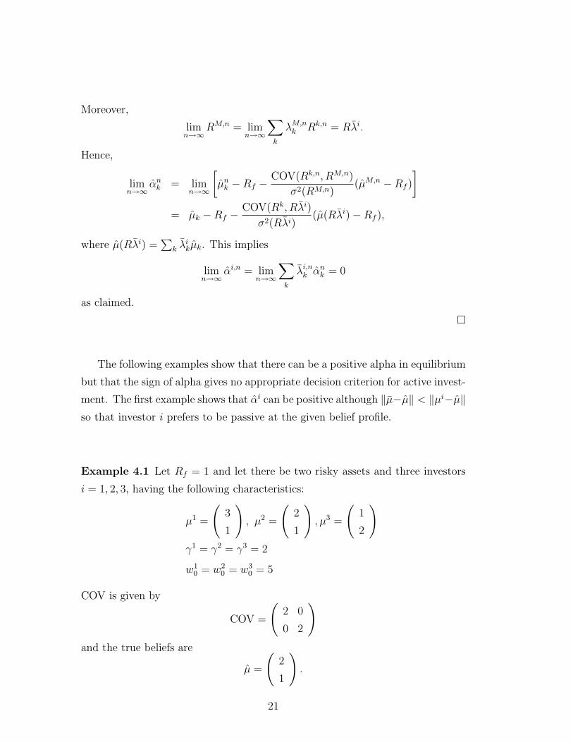
Moreover,

limn→∞

RM,n = limn→∞

∑

k

λM,nk Rk,n = Rλi.

Hence,

limn→∞

αnk = lim

n→∞

[µn

k −Rf − COV(Rk,n, RM,n)

σ2(RM,n)(µM,n −Rf )

]

= µk −Rf − COV(Rk, Rλi)

σ2(Rλi)(µ(Rλi)−Rf ),

where µ(Rλi) =∑

k λikµk. This implies

limn→∞

αi,n = limn→∞

∑

k

λi,nk αn

k = 0

as claimed.

¤

The following examples show that there can be a positive alpha in equilibrium

but that the sign of alpha gives no appropriate decision criterion for active invest-

ment. The first example shows that αi can be positive although ‖µ−µ‖ < ‖µi−µ‖so that investor i prefers to be passive at the given belief profile.

Example 4.1 Let Rf = 1 and let there be two risky assets and three investors

i = 1, 2, 3, having the following characteristics:

µ1 =

(3

1

), µ2 =

(2

1

), µ3 =

(1

2

)

γ1 = γ2 = γ3 = 2

w10 = w2

0 = w30 = 5

COV is given by

COV =

(2 0

0 2

)

and the true beliefs are

µ =

(2

1

).

21

Suppose now that all investors are active. We have a1 = a2 = a3 = 1/3 and

hence

µ = a1µ1 + a2µ2 + a3µ3 =

(243

).

We obtain‖µ− µ1‖2 = 1

2,

‖µ− µ2‖2 = 0,

‖µ− µ3‖2 = 1,

‖µ− µ‖2 = 116

.

Hence, investors 1 and 3 prefer to be passive for all costs K1, respectively, K3.

Nevertheless, investor 1 generates a positive alpha when he is active:

The optimal portfolios of the investors (everyone is active!) are

λ1 =

(12

0

), λ2 =

(14

0

), λ3 =

(014

).

Hence,

λ1 = λ2 =

(1

0

), λ3 =

(0

1

)

and the market portfolio is

λM =∑

i

riλi =

(3414

),

and hence

βM =COVλM

(λM)T COVλM=

(6525

).

This implies

α = µ−Rfe− βM(µM −Rf ) =

(110

− 310

),

from which we compute

α1 = αT λ1 = 1/10,

α2 = αT λ2 = 1/10,

α3 = αT λ3 = −3/10.

Hence, we see that investor 1 generates a positive alpha by being active although

he prefers to be passive.

22

The second example shows that αi can be negative although ‖µ− µ‖ > ‖µi−µ‖.

Example 4.2 Let the asset market structure be the same as in the previous

example. Let there be four investors i = 1, 2, 3, 4, having the following character-

istics:

µ1 =

(6

1

), µ2 =

(3

2

), µ3 =

(2

3

), µ4 =

(1

5

)

γ1 = γ2 = γ3 = γ4 = 2

w10 = w2

0 = w30 = w4

0 = 10

The true beliefs are

µ =

(2

2

).

Suppose now that all investors are active. We have a1 = a2 = a3 = a4 = 1/4

and hence

µ = a1µ1 + a2µ2 + a3µ3 + a4µ4 =

(3114

).

We obtain‖µ− µ1‖2 = 17

2,

‖µ− µ2‖2 = 12,

‖µ− µ3‖2 = 12,

‖µ− µ4‖2 = 5,

‖µ− µ‖2 = 2532

.

Hence, investors 2 and 3 prefer to be active for all costs K2, respectively, K3.

Nevertheless, investor 2 generates a negative alpha when he is active:

The optimal portfolios of the investors (everyone is active!) are

λ1 =

(54

0

), λ2 =

(1214

), λ3 =

(1412

), λ4 =

(0

1

).

23

Hence,

λ1 =

(1

0

), λ2 =

(2313

), λ3 =

(1323

), λ4 =

(0

1

)

and the market portfolio is

λM =∑

i

riλi =

(815715

),

and hence

βM =COVλM

(λM)T COVλM=

(110113105113

).

This implies

α = µ−Rfe− βM(µM −Rf ) =

(− 7

1138

113

),

from which we compute

α1 = αT λ1 = − 7113

,

α2 = αT λ2 = − 2113

,

α3 = αT λ3 = 3113

,

α4 = αT λ4 = 8113

Hence, we see that investor 2 generates a negative alpha by being active although

he prefers to be active if his costs K i are sufficiently small.

24

References

Agarwal, V., N. D. Daniel, and N. Y. Naik (2005): “Role of Managerial

Incentives, Flexibility and Ability: Evidence from Performance and Money

Flows in Hedge Funds,” mimeo, Georgia State University and London Business

School.

Berk, J. B., and R. C. Green (2004): “Mutual Fund Flows and Performance

in Rational Markets,” Journal of Political Economy, 112, 1269–1295.

Brock, W. A., and C. H. Hommes (1998): “Heterogeneous Beliefs and Routes

to Chaos in a Simple Asset Pricing Model,” Journal of Economic Dynamics

and Control, 22, 1235–1274.

Chopra, V. K., and W. T. Ziemba (1993): “The Effect of Errors in Mean,

Variance and Co-Variance Estimates on Optimal Portfolio Choice,” Journal of

Portfolio Management, 19, 6–11.

Getmansky, M. (2004): “The Life Cycle of Hedge Funds: Fund Flows, Size

and Performance,” mimeo, MIT Sloan School of Management.

Goetzmann, W. N., and A. Kumar (2005): “Why Do Individual

Investors Hold Under-Diversified Portfolios?,” Yale School of Manage-

ment Working Papers ysm454, Yale School of Management, available at

http://ideas.repec.org/p/ysm/somwrk/ysm454.html.

Grinold, R. C., and R. N. Kahn (2000): Active Porfolio Management: A

Quantitative Approach for Providing Superior Returns and Controlling Risk.

McGraw-Hill, New York.

Grossman, S. J., and J. E. Stiglitz (1980): “On the Impossibility of Infor-

mationally Efficient Markets,” American Economic Review, 70, 393–408.

Lintner, J. (1969): “The Aggregation of Investor’s Diverse Judgments and

Preferences in Purely Competitive Security Markets,” Journal of Financial

and Quantitative Analysis, 4, 347–400.

25

Litterman, R. (2003): “Why an Equilibrium Approach?,” in Modern Invest-

ment Management: An Equilibrium Approach, ed. by B. Litterman, and the

Quantitative Research Group Goldman Sachs Asset Management, chap. 1, pp.

3–6. Wiley, Hoboken, New Jersey.

Odean, T. (1999): “Do Investors Trade Too Much,” The American Economic

Review, 89, 1279–1298.

Polkovnichenko, V. (2005): “Household Portfolio Diversification: A Case

for Rank Dependent Preferences,” The Review of Financial Studies, 18, 1467–

1502.

26